CITY OF CHARLESTON, SOUTH CAROLINAMUNICIPAL FOREST RESOURCE ANALYSIS

BY

E. GREGORY MCPHERSON

JAMES R. SIMPSON

PAULA J. PEPER SHELLEY L. GARDNER

KELAINE E. VARGAS

JAMES HO

SCOTT MACO

QINGFU XIAO

CENTER FOR URBAN FOREST RESEARCH

USDA FOREST SERVICE, PACIFIC SOUTHWEST RESEARCH STATION

TECHNICAL REPORT TO:DANNY BURBAGE, URBAN FORESTRY SUPERINTENDENT

URBAN FORESTRY DIVISION, DEPARTMENT OF PARKS

CHARLESTON, SOUTH CAROLINA

—JULY 2006—

Mission Statement

We conduct research that demonstrates new ways in which treesadd value to your community, converting results into financial terms

to assist you in stimulating more investment in trees.

Investment Value

Energy Conservation

Air Quality

Water Quality

Firewise Landscapes

Areas of Research:

The United States Department of Agriculture (USDA) prohibits discrimination in all its programs and activities on the basis of race, color, national origin, gender, religion, age, disability,

political beliefs, sexual orientation and marital or family status. (Not all prohibited bases apply to all programs.) Persons with disabilities who require alternative means for communication

of program information (Braille, large print, audio-tape, etc.) should contact USDA’s TARGET Center at: (202) 720-2600 (voice and TDD).To file a complaint of discrimination, write:

USDA Director, Office of Civil Rights, Room 326-W,Whitten Building, 14th and Independent Avenue, SW,Washington, DC 20250-9410, or call: (202) 720-5964 (voice or TDD).

USDA is an equal opportunity provider and employer.

CITY OF CHARLESTON, SOUTH CAROLINAMUNICIPAL FOREST RESOURCE ANALYSIS

Technical report to: Danny Burbage

Urban Forestry SuperintendentCity of Charleston, SC

ByE. Gregory McPherson1

James R. Simpson1

Paula J. Peper1

Shelley L. Gardner1

Kelaine E. Vargas1

James Ho1

Scott Maco1

Qingfu Xiao2

—July 2006—

1Center for Urban Forest ResearchUSDA Forest Service, Pacifi c Southwest Research Stationc/o Dept. of Plant Science, MS-6University of CaliforniaOne Shields Ave.Davis, CA 95616-8587

2Department of Land, Air, and Water ResourcesUniversity of CaliforniaDavis, CA

AcknowledgementsWe appreciate the assistance provided by Danny Burbage (Urban Forestry Superintendent, City of Charleston, SC); Greg Ina, Jim Jenkins, and Karen Wise (Davey Resource Group); John L. Schrenk (SC Dept. of Health & Environmental Control); Jason Caldwell and Wes Tyler (SC Dept. of Natural Resourc-es); Ilya Bezdezhskiy, Stephanie Louie, and Stephanie Huang (CUFR).

Dr. Timothy Broschat (University of Florida, Ft. Lauderdale), Joe Le Vert (Southeastern Palm Society), and Ollie Oliver (Palm Trees, Ltd.) provided valuable assistance with calculating palm growth.

Mark Buscaino, Ed Macie (USDA Forest Service, State and Private Forestry), and Liz Gilland (U&CF Program Coordinator SC Forestry Commission) provided invaluable support for this project.

Table of Contents

Acknowledgements 2

Executive Summary 5Resource Structure 5Resource Function and Value 6

Resource Management Needs 7Chapter One—Introduction 9

Chapter Two—Charleston’s Municipal Tree Resource 11Tree Numbers 11Species Richness, Composition And Diversity 13Species Importance 13Street Tree Stocking Level 14

Street Trees Per Capita 14Age Structure 15Tree Condition 15Tree Canopy 15Maintenance Needs 16Replacement Value 17

Chapter Three—Costs of Managing Charleston’s Municipal Trees 19Tree Planting and Establishment 19Pruning, Removals, and General Tree Care 19Administration 20Other Tree-Related Expenditures 20

Chapter Four—Benefi ts of Charleston’s Municipal Trees 21Energy Savings 21

Electricity and Natural Gas Results 22Atmospheric Carbon Dioxide Reductions 22

Carbon Dioxide Reductions 22Air Quality Improvement 23

Deposition and Interception 23Avoided Pollutants 23BVOC Emissions 25Net Air Quality Improvement 25

Stormwater Runoff Reductions 25Aesthetic, Property Value, Social, Economic and Other Benefi ts 26Total Annual Net Benefi ts and Benefi t–Cost Ratio (BCR) 26

Chapter Five—Management Implications 29Resource Complexity 29Resource Extent 30Maintenance 30

Chapter Six—Conclusion 31

Appendix A—Tree Distribution 32

Appendix B—Replacement Values 36

Appendix C—Methodology and Procedures 39Growth Modeling 39Replacement Value 40Identifying and Calculating Benefi ts 41

Energy Savings 41Atmospheric Carbon Dioxide Reduction 48Improving Air Quality 48Reducing Stormwater Runoff 49Property Value and Other Benefi ts 50

Estimating Magnitude of Benefi ts 52Categorizing Trees by DBH Class 52Applying Resource Units to Each Tree 52Matching Signifi cant Species with Modeled Species 53Grouping Remaining “Other” Trees by Type 53Calculating Net Benefi ts And Benefi t–Cost Ratio 53Net Benefi ts and Costs Methodology 54

References 55

5

Executive Summary

Charleston, a charming Southern city appreciated for its rich history and culture, maintains trees as an integral component of the urban infrastructure (Figure 1). Research indicates that healthy trees can lessen impacts associated with the built envi-ronment by reducing stormwater runoff, energy consumption, and air pollutants. Trees improve ur-ban life, making Charleston a more enjoyable place to live, work, and play, while mitigating the city’s environmental impact. Over the years, the people of Charleston have invested millions of dollars in their municipal forest. The primary question that this study asks is whether the accrued benefi ts from Charleston’s municipal forest justify the annual ex-penditures?

This analysis combines results of a citywide inven-tory with benefi t–cost modeling data to produce four types of information on the tree resource:

• Structure (species composition, diversity, age distribution, condition, etc.)

• Function (magnitude of annual environmental and esthetic benefi ts)

• Value (dollar value of benefi ts minus manage-ment costs)

• Management needs (sustainability, planting, maintenance)

Resource Structure

The city’s tree inventory includes 15,244 publicly managed trees along the streets in Charleston. The inventory does not include and estimated 35,000 other trees located in parks, traffi c medians, wood-ed buffers and drainage areas. This assessment fo-cuses on the 15,244 trees that have been invento-ried and may therefore understate the full extent and benefi t of Charleston’s entire municipal forest.

Figure 1—Trees shade a historic home in Charleston, South Carolina. Public trees in Charleston provide great ben-efi ts, improving air quality, sequestering carbon dioxide, reducing stormwater runoff and beautifying the city. The trees of Charleston return $1.34 in benefi ts for every $1 spent on tree care.

6

There is approximately one public tree for every seven residents, and these public trees shade ap-proximately 0.24% of the city. Charleston’s streets are planted at near capacity, with 80% of possible planting spaces fi lled.

The inventory contains 136 tree species with Southern live oak (Quercus virginiana), crape-myrtle (Lagerstroemia indica) and sabal palmetto (Sabal palmetto) as the dominant species. These three species represent 64% of all street trees in Charleston and provide 51% of benefi ts.

The age structure of Charleston’s municipal tree population appears fairly close to “ideal.” A recent emphasis on new plantings means that there are many trees (nearly 50%) in the smallest size class (0–6 inch diameter at breast height or 4.5 ft above the ground [DBH]). The larger size classes are also well represented, while the 6–12 inch DBH class shows a marked dip with only 15% of trees in this class. Closer inspection at the management zone and species level shows a less desirable picture. Some areas have a high proportion of trees in the largest size classes, while others are represented almost entirely by small trees. As well, some spe-cies have a desirable age distribution while others include only young or only old trees.

Resource Function and Value

The ability of Charleston’s municipal trees to in-tercept rain—thereby reducing stormwater run-off—is substantial, estimated at 3.98 million cubic ft annually, or $171,406. Citywide, the average tree intercepts 1,858 gallons of stormwater each year, valued at $11 per tree.

Electricity saved annually in Charleston from both shading and climate effects of trees totals 1,039 MWh ($97,020) and annual natural gas saved to-tals 2,002 Mbtu ($23,971) for a total energy cost savings of $120,991 or $8 per tree.

Citywide, annual carbon dioxide (CO2) sequestra-tion and emission reductions due to energy savings by public trees are 944 tons and 711 tons, respec-tively. CO2 released during decomposition and

tree-care activities is relatively low (91 tons). Net CO2 reduction is 1,563 tons, valued at $23,452 or $1.54 per tree.

Net annual air pollutants removed, released, and avoided average 0.46 lb per tree and are valued at $36,270 or $0.43 per tree. Ozone is the most signif-icant pollutant intercepted by trees, with 6,104 lbs per year removed from the air, while sulfur dioxide is the most important air pollutant whose produc-tion is avoided at the power plant, due to reduced energy needs (8,104 lbs per year).

The estimated total annual benefi ts associated with aesthetics, property value increases, and other less tangible improvements are approximately $395,000 or $26 per tree on average.

Annual benefi ts total $717,034 and average $47 per tree. The 3,632 live oaks produce the highest total level of benefi ts among street trees ($84 per tree, 43% of total benefi ts). On a per tree basis, water oaks and laurel oaks are most important, providing an average of $156 and $133 per tree, respectively. Although together these two species make up less than 10% of the population, because of their great size and leaf area, they provide 27.6% of the total benefi ts. Nonetheless, despite the water oak’s high level of benefi ts, the species is not well suited as a street tree as it is short-lived, shallow-rooted and prone to failure. Species providing the least bene-fi ts on an individual tree basis include crapemyrtle ($8) and dogwood ($10).

Charleston spends approximately $700,000 annu-ally maintaining its public trees. For the purposes of this study, it was assumed that 75% of the bud-get ($531,200) is spent on the 15,244 trees in the inventory, or $35 per tree. Expenditures for prun-ing account for about one-half of total costs. Plant-ing represents another one-fi fth.

Charleston’s municipal trees are a valuable asset, providing approximately $185,834 or $12 per tree ($2/capita) in net annual benefi ts to the commu-nity. Over the years, Charleston has invested mil-lions in its urban forest. Citizens are now receiving a return on that investment—trees are providing

7

$1.35 in benefi ts for every $1 spent on tree care. Charleston’s benefi t–cost ratio of 1.35 is similar to that reported for Berkeley, CA (1.37), and exceeds that of San Francisco (1.00), but is lower than other cities, including Charlotte, NC (3.25), Glendale, AZ (2.41), Fort Collins, CO (2.18), Cheyenne, WY (2.09), and Minneapolis, MN (1.57) (McPherson et al. 2003, 2004b, 2005a–f).

The mild climate and clean air of the Charleston area are a partial explanation for the lower benefi ts of trees. Another possible factor is the predomi-nance of crapemyrtles and sabal palmettos. These species, which make up 40% of the population, have smaller leaf areas and return far fewer ben-efi ts on a per tree basis. Of course, in a historic city like Charleston, high building density and narrow streets mean smaller species are sometimes the best or only choice.

Continued investment in management and careful consideration of the future structure of the urban forest are critical to insuring that residents receive a high return on their investment.

Resource Management Needs

Charleston’s municipal trees are a dynamic re-source. Managers of the urban forest and the com-munity alike can take pride in knowing that munic-ipal trees do improve the quality of life in Charles-ton; the resource, however, is fragile and needs constant care to maximize and sustain the benefi ts through the foreseeable future. Achieving resource sustainability requires that Charleston:

• Continue to diversify the mix of tree species planted to guard against catastrophic losses due to storms, pests or disease.

• Sustain an annual planting program over the long-term to increase age diversity.

• Sustain benefi ts by investing in intensive main-tenance of mature trees to prolong the func-tional life spans of these heritage trees.

• Develop a strong young-tree-care program that

includes inspection and pruning on a two-year cycle.

• Plant large species where conditions are suit-able to maximize benefi ts.

• Insure adequate space for large trees in new de-velopments by revising street design standards. Encourage the use of structural soils where ap-propriate. Where possible, locate power lines belowground.

• Review and revise parking lot shade guidelines and the adequacy of current ordinances to pre-serve and protect large trees from development impacts.

These recommendations build on a history of civ-ic commitment to tree management that has put Charleston on course to provide an urban forest resource that is both functional and sustainable. As the city continues to grow, it must also continue to invest in its tree canopy. This is no easy task, given fi nancial constraints and trends toward increased development that put trees at risk.

The challenge ahead is to better integrate the green infrastructure with the gray infrastructure. This can be achieved by including green space and trees in the planning phase of development projects, pro-viding adequate space for trees, and designing and maintaining plantings to maximize net benefi ts over the long term. By acting now to implement these recommendations, Charleston will benefi t from a more functional and sustainable urban for-est in the future.

8

Figure 2—Stately oaks shade a park gazebo in Charleston.

9

Charleston is a charming, vibrant Southern city, ap-preciated for its rich history and cultural wealth. Trees are maintained as an integral component of the urban infrastructure (Figure 2) and have long been beloved and cared for by the city’s residents. The city’s Urban Forestry Division of the Depart-ment of Parks actively manages more than 50,000 trees along streets, in parks, in wooded buffers and drainage easements. The City believes that the public’s investment in stewardship of the urban forest produces benefi ts that far outweigh the costs to the community. Investing in Charleston’s green infrastructure makes sense economically, environ-mentally, and socially.

Research indicates that healthy city trees can mitigate impacts associated with urban environs: polluted storm-water runoff, poor air quality, high requirements for energy for heating and cooling buildings, and heat is-lands. Healthy public trees increase real estate values, provide neighbor-hood residents with a sense of place, and foster psychological, social, and physical health. Street and park trees are associated with other intangibles, too, such as increasing community attractiveness for tourism and busi-ness and providing wildlife habi-tat and corridors. The urban forest makes Charleston a more enjoyable place to live, work and play, while mitigating the city’s environmental impact (Figure 3).

In an era of decreasing public funds and rising costs, however, there is a need to scrutinize public expen-ditures that are often viewed as “nonessential,” such as planting and maintaining street and park trees. Although the current program has demonstrated its economic effi cien-cy, questions remain regarding the

need for the level of service presently provided. Hence, the primary question that this study asks is whether the accrued benefi ts from Charleston’s ur-ban trees justify the annual expenditures?

In answering this question, information is provided to do the following:

• Assist decision-makers to assess and justify the degree of funding and type of management program appropriate for Charleston’s urban forest.

• Provide critical baseline information for evalu-ating program cost-effi ciency and alternative management structures.

Chapter One—Introduction

Figure 3—Sabal palmettos, the State Tree of South Carolina, enliven Charleston’s historic Queen Street.

10

• Highlight the relevance and relationship of Charleston’s municipal tree resource to local quality of life issues such as environmental health, economic development, and psycho-logical health.

• Provide quantifi able data to assist in develop-ing alternative funding sources through utility purveyors, air quality districts, federal or state agencies, legislative initiatives, or local assess-ment fees.

This report consists of six chapters and three ap-pendices:

Chapter One—Introduction: Describes the pur-pose of the study.

Chapter Two—Charleston’s Municipal Tree Re-source: Describes the current structure of the street tree resource.

Chapter Three—Costs of Managing Charleston’s Municipal Trees: Details management expendi-tures for publicly managed trees.

Chapter Four—Benefi ts of Charleston’s Munici-pal Trees: Quantifi es the estimated value of tangi-ble benefi ts and calculates net benefi ts and a ben-efi t–cost ratio.

Chapter Five—Management Implications: Evalu-ates relevancy of this analysis to current programs and describes management challenges for street tree maintenance.

Chapter Six—Conclusions: Final word on the use of this analysis.

Appendix A—Tree Distribution: Lists species and numbers of trees in the population of street trees.

Appendix B—Replacement Values: Lists replace-ment values for the entire street tree population.

Appendix C—Describes procedures and method-ology for calculating structure, function, and value of the urban tree resource.

References—Lists publications cited in the study.

11

Chapter Two—Charleston’s Municipal Tree Resource

As might be expected in a city that includes the oldest landscaped gardens in the United States, the citizens of Charleston are passionate about their trees, believing that they add character, beauty, and serenity to the city. Sabal palmettos (Sabal pal-metto), the state tree, line the brick streets of the historic district and are renowned in Charleston’s history for helping to defeat the British during the Revolutionary War—the spongy logs of the make-shift fort on Sullivan’s Island absorbed the impact of cannonballs without splintering and breaking. Southern live oaks, draped with Spanish moss, form a living canopy over the streets of the city. Charleston is also home to the Angel Oak, a South-ern live oak (Quercus virginiana) estimated to be more than 1,400 years old (Figure 4). The Angel Oak has cast its 17,000 square feet of shade over performances by the Charleston Ballet Theatre, the Charleston Symphony Orchestra and over count-less more-humble picnics.

Tree Numbers

The Charleston street tree inventory was begun in 1992 and included 15,244 trees at the time of this study. Charleston’s Urban Forestry Division is also responsible for an additional estimated 35,000 trees, most of which are located in drainage ease-ments and wooded buffers.

The street tree population is dominated by broad-leaf trees (75% of the total; Table 1). Because broadleaf trees are usually larger than coniferous trees or palms and most of the benefi ts provided by

Tree type Number % of totalBroadleaf deciduous 7,047 46.2Broadleaf evergreen 4,355 28.6Coniferous 597 3.9Palm 3,245 21.3Total 15,244

Table 1—Street tree percentages by tree type.

Figure 4—Charleston’s Angel Oak, a Southern live oak estimated to be 1,400 years old.

12

Table 2—Most abundant street tree species in order of predominance by DBH class and tree type.

Species 0–3 3–6 6–12 12–18 18–24 24–30 30–36 36–42 >42 Total % of total

Broadleaf deciduous large (BDL)Water oak 11 19 53 161 278 200 51 8 1 782 5.1 Laurel oak 8 33 37 118 177 136 57 23 9 598 3.9 Red maple 43 92 12 4 4 - - - - 155 1.0 BDL other 158 456 164 88 70 41 21 19 6 1,023 6.7 Total 220 600 266 371 529 377 129 50 16 2,558 16.8 Broadleaf deciduous medium (BDM)BDM other 182 323 78 43 20 9 2 - - 657 4.3Total 182 323 78 43 20 9 2 - - 657 4.3 Broadleaf deciduous small (BDS)Crapemyrtle 1,568 1,025 418 45 2 - - - - 3,058 20.1 Flowering dogwood 138 122 86 7 - - - - - 353 2.3 BDS other 283 114 20 3 - 1 - - - 421 2.8 Total 1,989 1,261 524 55 2 1 - - - 3,832 25.1 Broadleaf evergreen large (BEL)Live oak 809 1,235 542 260 223 233 163 111 56 3,632 23.8 BEL other - 1 - - - - - - - 1 - Total 809 1,236 542 260 223 233 163 111 56 3,633 23.8 Broadleaf evergreen medium (BEM)BEM other 106 51 50 41 13 2 1 1 - 265 1.7Total 106 51 50 41 13 2 1 1 - 265 1.7 Broadleaf evergreen small (BES)BES other 265 134 49 9 - - - - - 457 3.0Total 265 134 49 9 - - - - - 457 3.0 Conifer evergreen large (CEL)Loblolly pine 9 15 60 99 63 24 3 1 - 274 1.8 CEL other 26 22 40 36 19 10 1 - 1 155 1.0 Total 35 37 100 135 82 34 4 1 1 429 2.8 Conifer evergreen medium (CEM)CEM other 64 67 15 13 7 2 - - - 168 1.1Total 64 67 15 13 7 2 - - - 168 1.1 Conifer evergreen small (CES)CES other - - - - - - - - - - -Total - - - - - - - - - - -Palm evergreen large (PEL)PEL other 2 2 - - - - - - - 4 -Total 2 2 - - - - - - - 4 - Palm evergreen medium (PEM)Sabal palmetto 3 49 558 2,324 54 - - - - 2,988 19.6 PEM other 2 4 2 - - - - - - 8 0.1 Total 5 53 560 2,324 54 - - - - 2,996 19.7 Palm evergreen small (PES)Jelly palm 4 11 39 92 74 3 - - - 223 1.5 PES other 9 5 1 7 - - - - - 22 0.1 Total 13 16 40 99 74 3 - - - 245 1.6 Citywide total 3,690 3,780 2,224 3,350 1,004 661 299 163 73 15,244

13

trees are related to leaf surface area, broadleaf trees usually provide the highest level of benefi ts. Of the broadleaf trees, approximately 40% are evergreen. The presence of leaves on the trees year-round adds to their value in terms of stormwater interception, air pollutant uptake, and carbon dioxide seques-tration. Palms make up one-fi fth of the street tree population and conifers, the remaining 4%.

Species Richness, Composition And Diversity

The tree population in Charleston includes a rich mix 136 different species—more than twice the mean of 53 species reported by McPherson and Rowntree (1989) in their nationwide survey of street tree populations in 22 U.S. cities. The mild climate of the Coastal Plain and the city’s long his-tory of lush, carefully tended gardens, some dating back to the late 17th century, play a role in this spe-cies richness.

The predominant street tree species are live oak (23.8%), crapemyrtle (Lagerstroemia spp., 20.1%), and sabal palmetto (19.6%) (Table 2). Taken to-gether, these three species represent 64% of the street trees in Charleston, and all exceed the gener-al rule that no single species should represent more than 10% of the population and no genus more than 20% (Clark et al. 1997).

Dominance of this kind is of concern because of the impact that drought, disease, pests, or other stress-

ors can have on the urban forest. Although live oaks, crapemyrtles, and sabal palmettos are gener-ally not susceptible to pests and disease, nonnative fungi and insects have caused serious unexpected damage to other species in the past. On the other hand, live oaks and sabal palmettos are among the most hurricane-resistant of all trees, withstanding the winds of the worst hurricanes to hit the south-eastern United States (Duryea et al. 1996; Duryea 1997; Touliatos and Roth 1971).

At the management zone level, the problem of overly dominant species is exacerbated (Table 3). In James Island, for instance, nearly half of all street trees are crapemyrtles. In the Broad-Calhoun and South of Broad areas, sabal palmettos represent one-third of street tree plantings. In these cases, in addition to the dangers of catastrophic loss due to pests or disease, there should be concern over lost benefi ts, as small trees and palms have less leaf surface area and provide fewer benefi ts than large trees. In historic cities, of course, space for trees is at a premium, and small trees and palms are some-times the only option.

Species Importance

Importance values (IV) are particularly meaningful to managers because they indicate a community’s reliance on the functional capacity of particular species. For this study, IV takes into account not only total tree numbers, but canopy cover and leaf

Zone 1st (%) 2nd (%) 3rd (%) 4th (%) 5th (%)

Broad - Calhoun Sabal palmetto (34.7) Live oak (18.6) Crapemyrtle (17.6) Water oak (2.9) Laurel oak (2.7)

Calhoun - Crosstown Live oak (26.5) Sabal palmetto (22.3) Crapemyrtle (22.1) Water oak (3.3) Dogwood (2.3)

Crosstown - City limits Live oak (30) Crapemyrtle (18) Sabal palmetto (16.5) Water oak (8) Laurel oak (4.8)

Daniel Island Live oak (27.4) Crapemyrtle (13.2) London plane (8.3) Chinese pistache (7.9) Sabal palmetto (6.9)

Hampton Park Terrace Live oak (27.3) Crapemyrtle (23.9) Laurel oak (8.5) Sabal palmetto (7.9) Water oak (7.3)

Hwy 17 - Hwy 61 Live oak (34) Crapemyrtle (20.3) Sabal palmetto (11.5) Water oak (4.3) Laurel oak (4.1)

James Island Crapemyrtle (47.6) Live oak (29.2) Sabal palmetto (3.3) Dogwood (2.6) Jelly palm (2.2)

N of Hwy 61 Crapemyrtle (20.2) Live oak (15.9) Sabal palmetto (12.3) Loblolly pine (9) Jelly palm (6.3)

S of Hwy 61 Live oak (25.6) Crapemyrtle (19.1) Sabal palmetto (11.9) Water oak (8.4) Laurel oak (8.1)

South of Broad Sabal palmetto (33.4) Crapemyrtle (19.5) Live oak (15.7) Water oak (3.9) Laurel oak (3.3)

Wagener Terrace Live oak (23) Crapemyrtle (22.8) Water oak (9.5) Sabal palmetto (9.5) Laurel oak (6.4)

Citywide total Live oak (23.8) Crapemyrtle (20.1) Sabal palmetto (19.6) Water oak (5.1) Laurel oak (3.9)

Table 3—Most abundant tree species listed by management zone with percentage of totals in parenthesis.

14

area, providing a useful comparison to the total population distribution.

Importance value (IV), a mean of three relative val-ues, can, in theory, range between 0 and 100, where an IV of 100 implies total reliance on one species and an IV of 0 suggests no reliance. Street tree populations with one dominant species (IV>25%) may have low maintenance costs due to the effi -ciency of repetitive work, but may still incur large costs if decline, disease, or senescence of the domi-nant species results in large numbers of removals and replacements. When IVs are more evenly dis-persed among fi ve to ten leading dominant species the risks of a catastrophic loss of a single dominant species are reduced. Of course, suitability of the dominant species is an important consideration. Planting short-lived or poorly adapted species can result in short rotations and increased long-term management costs.

The nine most abundant street tree species listed in Table 4 constitute 79% of the total street tree population, 85% of the total leaf area, and 86% of total canopy cover, for an IV of 83.4. As Table 4 illustrates, Charleston is relying on the functional capacity of live oaks even more than their popula-tion numbers suggest. Though the species accounts for 23.8% of all public trees, because of the trees’ relatively large size, the amount of leaf area and canopy cover they provide is even greater, increas-ing their importance value to 33 when all compo-nents are considered. This makes them 2.5 times

more signifi cant than the next species. In contrast, small trees tend to have lower importance values than their population numbers would suggest. Al-though crapemyrtles make up 20% of the popula-tion, their IV is only 8.4.

Street Tree Stocking Level

The stocking level, or the ratio of planted trees to possible planting spaces, is an important way of measuring how well-forested a city is. It also serves as a helpful baseline for setting future goals. The stocking level in Charleston is not easy to es-timate. The inventory used for this project includes some sites identifi ed as available planting spaces for small species (106 sites) and existing stumps (89); both represent opportunities for planting, but there are certainly far more empty sites than these. A recent management plan for the city (Davey Re-source Group 2000) stated that there were 3,764 potential planting spaces. By this measure, Charles-ton’s street tree stocking level is 80%, a very high percentage.

Street Trees Per Capita

Calculation of street trees per capita is another way of describing how well-forested a city is. Assuming a human population of 104,883 and a tree popula-tion of 15,244 (Burbage 2005), Charleston’s num-ber of street trees per capita is 0.15—approximate-ly one tree for every seven people—signifi cantly below the mean ratio of 0.37 reported for 22 U.S. cities (McPherson and Rowntree 1989).

Table 4—Importance values (IV) indicate which species dominate the population due to their numbers and size.

Species No. of trees

% of total trees

Leaf area (ft2)

% of total leaf area

Canopy cover (ft2)

% of total canopy cover

I V

Live oak 3,632 23.8 5,390,199 38.3 2,633,361 37.7 33.3Crapemyrtle 3,058 20.1 135,581 1.0 291,091 4.2 8.4Sabal palmetto 2,988 19.6 1,205,900 8.6 732,614 10.5 12.9Water oak 782 5.1 2,648,985 18.8 1,125,728 16.1 13.4Laurel oak 598 3.9 2,134,941 15.2 902,394 12.9 10.7Flowering dogwood 353 2.3 20,587 0.1 58,810 0.8 1.1Loblolly pine 274 1.8 317,560 2.3 203,621 2.9 2.3Jelly palm 223 1.5 57,088 0.4 39,969 0.6 0.8Red maple 155 1.0 31,146 0.2 27,382 0.4 0.5Total most abundant 12,063 79.1 11,941,987 85 6,014,970 86 83.4

15

Age Structure

The distribution of ages within a tree population infl uences present and future costs as well as the fl ow of benefi ts. An uneven-aged population allows managers to allocate annual maintenance costs uni-formly over many years and assures continuity in overall tree-canopy cover. An ideal distribution has a high proportion of new transplants to offset estab-lishment-related mortality, while the percentage of older trees declines with age (Richards 1982/83).

The overall age structure, represented here in terms of DBH, for street trees in Charleston appears quite similar to the ideal (Figure 5). Closer examination, however, shows that the results differ greatly by species. Live oak shows a desirable distribution across DBH classes. Other large-growing species are heavily represented in the smaller DBH classes, suggesting that the city has begun to plant some new large- and medium-growing species recently, including red maple (Acer rubrum) and Chinese pistache (Pistacia chinensis) (87.1 and 100% in the 0–6 inch DBH class, respectively). In contrast, oth-er species, such as laurel oak (Quercus laurifolia) and water oak (Quercus nigra), seem to have fallen out of favor with only 6.8 and 3.8% of their popula-tions, respectively, in the smallest DBH class.

A closer look at age distribution by management zone also presents an interesting picture (Figure 6).

Some areas, such as Wagener Terrace and Hamp-ton Park Terrace, have a large proportion of trees in the largest size classes. James Island and Daniel Island, in contrast, have most of their trees in the smallest size classes. In James Island, this can be partly explained by the fact that nearly half of their trees are crapemyrtles, which rarely grow beyond the 0–6 inch DBH class. The predominant species mix in Daniel Island, however, includes live oak, London plane (Platanus x acerifolia) and Chinese pistache. The age distribution therefore indicates increased planting efforts in recent years.

For many neighborhoods and for the city overall, there is a dip in the number of trees in the 6–12 inch DBH class. This may refl ect reduced planting rates in the 1990s, increased mortality levels, such as following Hurricane Hugo, or both.

Tree Condition

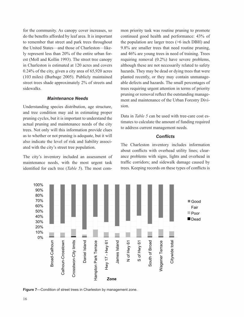
Tree condition indicates both how well trees are managed and how well they perform given site-specifi c conditions. Overall, the condition of trees in Charleston is very good, with 89% in good or fair shape (Figure 7).

Tree Canopy

Canopy cover, or more precisely, the amount and distribution of leaf surface area, is the driving force behind the urban forest’s ability to produce benefi ts

Figure 5—Relative age distribution for Charleston’s 8 most abundant street tree species citywide shown with an ideal distribution.

0-6

6-12

12-1

8

18-2

4

24-3

0

30-3

6

>36 Ideal

Citywide total

Crapemyrtle

Water oak

Laurel oak

Flowering dogwood

Loblolly pine

Red maple

Chinese pistache

Live oak0102030405060708090

100

DBH Class

(%)

0-6

6-12

12-1

8

18-2

4

24-3

0

30-3

6

36-4

2 Broad-Calhoun

Calhoun-Crosstown

Crosstown-City limits

Daniel Island

Hampton Park Terrace

Hwy 17 - Hwy 61

James Island

N of Hwy 61

S of Hwy 61

South of Broad

Wagener Terrace

Citywide total0

10

20

30

40

50

60

70

80

90

(%)

DBH Class

Figure 6—Relative age distribution of all street trees by management zone.

16

for the community. As canopy cover increases, so do the benefi ts afforded by leaf area. It is important to remember that street and park trees throughout the United States—and those of Charleston—like-ly represent less than 20% of the entire urban for-est (Moll and Kollin 1993). The street tree canopy in Charleston is estimated at 120 acres and covers 0.24% of the city, given a city area of 65,920 acres (103 miles) (Burbage 2005). Publicly maintained street trees shade approximately 2% of streets and sidewalks.

Maintenance Needs

Understanding species distribution, age structure, and tree condition may aid in estimating proper pruning cycles, but it is important to understand the actual pruning and maintenance needs of the city trees. Not only will this information provide clues as to whether or not pruning is adequate, but it will also indicate the level of risk and liability associ-ated with the city’s street tree population.

The city’s inventory included an assessment of maintenance needs, with the most urgent task identifi ed for each tree (Table 5). The most com-

mon priority task was routine pruning to promote continued good health and performance: 43% of the population are larger trees (>6 inch DBH) and 9.8% are smaller trees that need routine pruning, and 46% are young trees in need of training. Trees requiring removal (0.2%) have severe problems, although these are not necessarily related to safety hazards. They may be dead or dying trees that were planted recently, or they may contain unmanage-able defects and hazards. The small percentages of trees requiring urgent attention in terms of priority pruning or removal refl ect the outstanding manage-ment and maintenance of the Urban Forestry Divi-sion.

Data in Table 5 can be used with tree-care cost es-timates to calculate the amount of funding required to address current management needs.

Confl icts

The Charleston inventory includes information about confl icts with overhead utility lines; clear-ance problems with signs, lights and overhead in traffi c corridors; and sidewalk damage caused by trees. Keeping records on these types of confl icts is

Figure 7—Condition of street trees in Charleston by management zone.

0%10%20%30%40%50%60%70%80%90%

100%

Bro

ad-C

alho

un

Cal

houn

-Cro

ssto

wn

Cro

sstw

on-C

ity li

mits

Dan

iel I

slan

d

Ham

pton

Par

k Te

rrac

e

Hw

y 17

- H

wy

61

Jam

es Is

land

N o

f Hw

y 61

S o

f Hw

y 61

Sou

th o

f Bro

ad

Wag

ener

Ter

race

City

wid

e to

tal

Zone

GoodFairPoorDead

17

helpful in planning future maintenance and can be very useful in understanding which species are best suited to certain sites. Table 6 describes confl icts for the most predominant species.

Replacement Value

Replacement value is a way of describing the cur-rent value of trees, refl ecting their current number, stature, placement, and condition. There are sev-eral methods that arborists employ to develop a fair and reasonable perception of a tree’s value (CTLA 1992, Watson 2002). The cost approach is widely used today and assumes that value equals the cost of production, or in other words, the cost of replac-ing a tree in its current state (Cullen 2002).

Replacing Charleston’s 15,244 street trees with trees of similar size, species, and condition if,

for example, all were destroyed by a catastrophic storm, would cost approximately $42.5 million (Table 7). The average replacement value per tree is $2,788. Live oaks account for almost 50% of the population’s total replacement value, with most of this value in the older and larger trees. Charleston’s street trees are a valuable legacy. As a central com-ponent of the city’s green infrastructure, these street trees are an asset valued at $42.5 million.

Replacement value should be distinguished from the value of annual benefi ts produced by the urban forest. The latter will be described in Chapter 4, as a “snapshot” of benefi ts during one year, while the former accounts for the his-torical investment in trees over their lifetimes. Hence, the replacement value of Charleston’s street tree population is many times greater than the value of annual benefi ts it produces.

Maintenance type 0–3 3–6 6–12 12–18 18–24 24–30 30–36 36–42 >42 Total % of pop’nPriority 1 - - - 2 8 6 3 - - 19 0.1Priority 2 - - 4 7 2 2 1 - - 16 0.1Removal 1 - 1 1 3 2 - - - - 7 0.0Removal 2 4 5 1 8 3 1 1 - - 23 0.2Routine prune 3 67 1,303 3,129 895 633 286 161 71 6,548 43.0Routine small prune 12 627 602 166 78 4 - - - 1,489 9.8Train 3,670 3,059 291 3 - - - - - 7,023 46.1Stump 1 21 21 29 16 14 8 2 2 114 0.7Boom - - 1 3 - 1 - - - 5 0.0Citywide total 3,690 3,780 2,224 3,350 1,004 661 299 163 73 15,244 100.0

Table 5—Maintenance needs by DBH class.

Species Power lines Comm. lines Power and comm. lines Sidewalk heave Lights SignsLive oak 349 186 1,084 2,822 21 395Crapemyrtle 150 146 1,117 2,722 13 215Sabal palmetto 151 127 737 2,661 2 9Water oak 56 27 331 630 1 48Laurel oak 48 29 295 523 0 58Flowering dogwood 21 23 165 289 0 18Jelly palm 40 0 38 36 0 6Other trees 232 129 944 2,667 37 178Citywide total 1,047 667 4,711 12,350 74 927

Table 6—Number of confl icts between trees and power lines, overhead communication lines, sidewalks, lights, and signs for the most common species in Charleston.

18

Species 0-3 3-6 6-12 12-18 18-24 24-30 30-36 36-42 >42 Total

Live oak 79,588 666,396 1,122,699 1,527,439 2,506,392 4,337,350 4,478,524 3,954,465 2,214,472 20,887,324

Water oak 1,739 8,860 82,594 596,516 2,069,399 2,521,279 911,086 156,486 3,844 6,351,803

Laurel oak 990 17,330 64,328 534,686 1,560,200 1,935,157 1,177,804 655,900 311,583 6,257,978

Crapemyrtle 172,835 542,299 820,276 243,048 20,260 - - - - 1,798,718

Loblolly pine 1,130 7,602 115,127 476,936 560,072 341,236 70,205 28,696 - 1,601,002

Southern red oak - 28,126 - 9,284 76,474 88,053 118,907 146,040 30,882 497,767

American sycamore 1,580 10,869 16,083 22,060 52,277 122,693 47,031 143,397 24,121 440,111

Southern magnolia 2,546 8,932 81,633 197,778 81,765 28,646 20,880 - - 422,181

Willow oak 466 32,814 57,744 36,291 60,207 69,266 85,363 31,184 34,859 408,193

Hackberry 946 1,151 40,066 113,370 116,366 77,825 24,703 - 25,788 400,215

Sweetgum 5,611 1,884 30,451 66,100 117,280 109,389 48,501 - - 379,215

Flowering dogwood 15,256 65,368 163,810 33,025 - - - - - 277,459

Pecan 377 2,022 13,530 53,103 87,753 47,837 21,682 28,696 - 255,000

Northern red oak - 58 1,174 429 23,383 8,056 39,971 74,705 54,677 202,452

Eastern red cedar 4,182 13,559 22,428 50,349 56,124 22,379 - - - 169,022

Sabal palmetto 60 1,203 21,117 132,186 4,177 - - - - 158,743

Honeylocust 2,033 11,789 83,220 53,581 - - - - - 150,622

American holly 2,200 27,350 70,068 42,673 - - - - - 142,291

Red maple 4,922 48,022 22,728 23,355 39,905 - - - - 138,933

Callery pear 4,248 13,201 15,822 42,064 7,388 - - - - 82,724

American elm - - - 6,340 22,086 23,006 9,304 9,857 - 70,593

Chinese elm 368 488 3,444 5,642 45,167 12,756 - - - 67,866

Darlington oak - - - - 25,810 - - 28,696 - 54,505

Baldcypress 550 8,637 29,388 15,585 - - - - - 54,160

Chinese pistache 5,763 46,133 - - - - - - - 51,896

Jelly palm 601 2,550 9,090 21,227 17,005 695 - - - 51,168

Tallowtree 3,184 8,412 20,086 19,184 - - - - - 50,866

Oct glory red maple 1,904 46,679 - - - - - - - 48,584

London planetree 2,813 44,685 - - - - - - - 47,498

Japanese zelkova 2,461 27,931 13,776 - - - - - - 44,168

Muskogee crapemyrtle 8,920 23,364 11,429 - - - - - - 43,713

Winged elm - - - 13,292 9,846 16,113 - - - 39,250

Shumard oak 4,179 32,462 - - - - - - - 36,641

Black oak - - - - 7,743 - - 28,696 - 36,439

White oak - - - 5,305 10,349 20,735 - - - 36,389

River birch 718 15,099 14,022 5,642 - - - - - 35,481

Carolina laurelcherry 3,182 7,266 7,945 10,903 5,863 - - - - 35,160

Siberian elm - - - 4,589 11,593 10,583 7,353 - - 34,118

Red mulberry - 943 8,349 5,065 8,906 10,303 - - - 33,565

Slash pine - - - 11,362 8,196 13,314 - - - 32,872

Other trees 92,046 153,321 121,831 105,075 82,339 15,535 - - - 570,147

Citywide total 427,399 1,926,806 3,084,259 4,483,482 7,694,324 9,832,209 7,061,316 5,286,815 2,700,224 42,496,834

Table 7—Replacement values, summed by DBH class, for the 40 most valuable species of street trees in Charleston. See Appendix B for complete listing.

19

Chapter Three—Costs of Managing Charleston’s Municipal Trees

The benefi ts that Charleston’s trees provide come, of course, at a cost. This chapter presents a break-down of annual expenditures for fi scal year 2004. Total annual tree-related expenditures for Charles-ton’s municipal forestry program are approxi-mately $700,000 (Table 8) (Burbage 2005). This amount represents 0.6% of Charleston’s total 2004 operating budget ($115 million) and $6/capita. The tree budget funds the care of more than the 15,244 trees included in the inventory; it includes an addi-tional estimated 35,000 trees in parks, traffi c medi-ans, wooded buffers and drainage easements. This study will only determine benefi ts for the invento-ried trees, therefore we consider only the portion of the budget that applies to trees in the inventory. Because the other 35,000 trees are in parks and other more “naturalized” areas, they require less maintenance than the street trees, and we therefore estimate that the inventoried trees consume about 75% of the tree care budget, or $531,200 (Burbage 2005). The numbers in the following sections rep-resent this proportion of the municipal tree care budget.

The city spends about $35 per tree on average during the fi scal year, signifi cantly greater than the 1997 mean value of $19 per tree reported for 256 Cali-fornia cities after adjusting for infl ation (Thompson and Ahern 2000). However, non-program expendi-tures (e.g., sidewalk repair, litter clean-up) were not included in the California survey. Charleston’s annual expenditure is approximately equal to that of Fort Collins, CO ($32), and far less than some California communities such as Santa Monica

($53) and Berkeley ($65) (McPherson et al. 2002, 2003, 2005f).

Forestry program expenditures fall into three gen-eral categories: tree planting and establishment, pruning and general tree care, and administration.

Tree Planting and Establishment

Quality nursery stock, careful planting, and fol-low-up care are critical to perpetuation of a healthy urban forest. By planting new trees that are rela-tively large, with DBH of 2.5–3 inches, the city of Charleston is giving its urban forest a healthy start. The Urban Forestry Division plants about 500 trees annually, with three trees planted for every one re-moved. Tree planting activities, including materi-als, labor, administration, and equipment costs, account for 20.5% of the program budget or ap-proximately $110,000.

An innovative tree planting program that brings to-gether the Urban Forestry Division and residents is partly responsible for the high number of new plantings. On request, residents receive a 2½–3 inch DBH tree at wholesale prices. The tree is planted by the city and the homeowner agrees to water it for the fi rst year. The effectiveness of this collaboration is also evident in the low establish-ment-related mortality of newly planted trees: less than 1% annually (Burbage 2005).

Pruning, Removals, and General Tree Care

Pruning accounts for nearly half of the annual ex-penditures at $243,750 ($16 per tree). This is partly

Table 8—Charleston’s annual municipal forestry-related expenditures.

Expenditures Total ($) $/Tree $/Capita % of total Purchasing trees and planting 109,125 7.16 1.04 20.5 Contract pruning 243,750 15.99 2.32 45.9 Tree & stump removal 23,625 1.55 0.23 4.4 Irrigation 4,700 0.31 0.04 0.9 Administration 60,000 3.94 0.57 11.3 Litter clean-up 45,000 2.95 0.43 8.5 Infrastructure repairs 45,000 2.95 0.43 8.5Total expenditures 531,200 34.85 5.06 100

20

a refl ection of the amount of care the sabal palmetto trees require for safety and aesthetics purposes. The tree maintenance crews spend nearly one-third of the year pruning the city’s 3,000 palmettos (Davey Resource Group 2000).

On average, new trees are trained once every three years. Small trees are pruned every six years and large trees every ten. The quality of the Urban For-estry Division’s pruning program is refl ected in the low number of trees requiring priority pruning (0.2%). Careful pruning is particularly important in such a hurricane-prone area.

Tree and stump removal accounts for only 4.4% of tree-related expenses ($23,625). About 70 street trees are removed each year. Most of the removed wood (85%) is disposed of in a landfi ll in order to control the spread of Formosan termites. Formosan termites are an invasive, nonnative species that fi rst appeared in the United States in Charleston in 1957. They eat more than 50 species of plants as well as lumber, mulch, asphalt, plastic and thin sheets of metal and can cause severe structural damage to a

house in less than two years (Forschler 2002). For these reasons, the Urban Forestry Division is care-ful to dispose of all potentially infested woody ma-terial.

Irrigation accounts for less than 1% of the budget ($4,700). New trees that are not planted in front of homes are irrigated for the fi rst year using a water truck. The city does not have any budgeted funds for pest and disease management.

Administration

An additional $60,000 is spent on administration expenses including supplies, travel, training, in-surance and workers’ compensation. Salaries for managers and clerical staff and overtime costs for hourly workers have been included in other cost categories.

Other Tree-Related Expenditures

In a typical year, Charleston spends about $45,000 on litter clean-up. This number includes overtime salaries for clean-up crews. In years with heavy storms, this number may be signifi cantly higher.

Annually, about $45,000 is spent by the city on infrastructure repair related to tree roots. Shallow roots that heave sidewalks, crack curbs, and dam-age driveways are an important aspect of mature tree care (Figure 8). The Division works closely with other departments to fi nd solutions to tree/sidewalk confl icts. Once problems occur, the city attempts to resolve them without removing the tree. Strategies include ramping the sidewalk over the root or moving the sidewalk around the tree, grinding concrete to level surfaces, removing and replacing concrete, and pruning roots only when necessary. Not all curb and sidewalk damage is due to tree roots, especially in historic parts of the city where infrastructure is old. However, infi ll and higher density development will increase tree root–hardscape confl icts unless structural soils, careful species selection, and other practices are used.

Figure 8—Confl icts between older trees and old infra-structure can be costly and diffi cult to repair, but the ben-efi ts provided by trees such as this one make the effort worthwhile.

21

Chapter Four—Benefi ts of Charleston’s Municipal Trees

City trees work ceaselessly, providing ecosys-tem services that directly improve human health and quality of life. In this section, the benefi ts of Charleston’s street trees are described. It should be noted that this is not a full accounting because some benefi ts are intangible or diffi cult to quantify (e.g., impacts on psychological and physical health, crime, and violence). Also, our limited knowledge about the physical processes at work and their inter-actions makes these estimates imprecise (e.g., fate of air pollutants trapped by trees and then washed to the ground by rainfall). Tree growth and mortali-ty rates are highly variable. A true and full account-ing of benefi ts and costs must consider variability among sites throughout the city (e.g., tree species, growing conditions, maintenance practices), as well as variability in tree growth.

Therefore, these estimates provide fi rst-order ap-proximations of tree value. Our approach is a gen-eral accounting of the benefi ts produced by mu-nicipal trees in Charleston—an accounting with an accepted degree of uncertainty that can nonetheless provide a platform from which decisions can be made (Maco and McPherson 2003). Methods used to quantify and price these benefi ts are described in more detail in Appendix C.

Energy Savings

Trees modify climate and conserve energy in three principal ways:

• Shading reduces the amount of radiant energy absorbed and stored by built surfaces.

• Transpiration converts moisture to water vapor and thus cools the air by using solar energy that would otherwise result in heating of the air.

• Wind-speed reduction reduces the movement of outside air into interior spaces and conduc-tive heat loss where thermal conductivity is relatively high (e.g., glass windows) (Simpson 1998).

Trees and other vegetation within building sites may lower air temperatures 5°F (3°C) compared to outside the greenspace (Chandler 1965) (Figure 9). At the larger scale of city-wide climate (6 miles or 10 km square), temperature differences of more than 9°F (5°C) have been observed between city centers and more vegetated suburban areas (Akbari et al. 1992). The relative importance of these ef-fects depends on the size and confi guration of trees and other landscape elements (McPherson 1993). Tree spacing, crown spread, and vertical distribu-tion of leaf area infl uence the transport of warm air and pollutants along streets and out of urban canyons.

Trees reduce air movement into buildings and con-ductive heat loss from buildings. Trees can reduce wind speed and resulting air infi ltration by up to 50%, translating into potential annual heating sav-

Figure 9 —Trees shade a Charleston neighborhood, re-ducing energy use for cooling and cleaning the air.

22

ings of 25% (Heisler 1986). Decreasing wind speed reduces heat transfer through conductive materials as well. Appendix C provides additional informa-tion on specifi c contributions that trees make to-ward energy savings.

Electricity and Natural Gas Results

Electricity and natural gas saved annually in Charleston from both shading and climate ef-fects total 1,039 MWh ($97,020) and 2,002 Mbtu ($23,971), respectively, for a total retail savings of $120,991 (Table 9) or a citywide average of $7.94 per tree. Water, laurel, and live oaks are the primary contributors to energy savings on a per tree basis.

Live oaks account for 23.8% of total tree num-bers, but provide 34.6% of the energy savings, as expected for a tree species with such a high Im-portance Value (IV). Water oaks and laurel oaks provide even greater energy savings on a per tree basis. One reason their contribution is greater than live oaks is because, as semi-deciduous trees, they block less of the winter sun’s warming rays and therefore do not have a negative effect on heat-ing costs, as live oaks, planted injudiciously, can. Crapemyrtles, in contrast, make up 20.1% of the population and provide less than 5% of energy sav-ings, consistent with their smaller IV.

Atmospheric Carbon Dioxide Reductions

Urban forests can reduce atmospheric carbon diox-ide in two ways:

• Trees directly sequester CO2 as woody and fo-liar biomass while they grow.

• Trees near buildings can reduce the demand for heating and air conditioning, thereby reducing emissions associated with electric power pro-duction and consumption of natural gas.

At the same time, however, CO2 is released by vehicles, chain saws, chippers, and other equip-ment during the process of planting and maintain-ing trees. Eventually, all trees die and most of the CO2 that has accumulated in their woody biomass is released into the atmosphere as they decompose unless recycled. These factors must be taken into consideration when calculating the carbon dioxide benefi ts of trees.

Carbon Dioxide Reductions

Citywide, Charleston’s municipal forest reduced atmospheric CO2 by a net of 1,563 tons annually (Table 10). This benefi t was valued at $23,452 or $1.54 per tree. Avoided CO2 emissions from power plants due to cooling energy savings totaled 711 tons, while CO2 sequestered by trees was 944 tons. CO2 released through decomposition and tree care activities totaled 91 tons, or 5.5% of the net total benefi t. Avoided emissions are important in Charleston because coal, which has a relatively high CO2 emissions factor, accounts for 66% of the fuel used in power plants that generate electricity there (US EPA 2003). Shading by trees during sum-

Table 9—Net annual energy savings produced by Charleston street trees.

Species Electricity (MWh)

Electricity ($)

Natural gas (MBtu)

Natural gas ($)

Total ($) % of total trees

% of total $

Avg. $/tree

Live oak 376 35,105 565 6,766 41,871 23.8 34.6 11.53Crapemyrtle 45 4,177 125 1,493 5,670 20.1 4.7 1.85Sabal palmetto 117 10,885 291 3,481 14,367 19.6 11.9 4.81Water oak 167 15,595 348 4,170 19,766 5 16.3 25.28Laurel oak 131 12,249 267 3,201 15,449 3.9 12.8 25.83Flowering dogwood 9 851 24 286 1,137 2.3 0.9 3.22Loblolly pine 32 3,015 63 749 3,764 1.8 3.1 13.74Jelly palm 6 595 13 162 756 1.5 0.6 3.39Red maple 6 523 10 124 647 1.0 0.5 4.18Other street trees 150 14,025 296 3,540 17,565 20.9 14.5 5.52Citywide total 1,039 97,020 2,002 23,971 120,991 100.0 100.0 7.94

23

mer reduces the need for air conditioning, resulting in reduced use of coal for electricity generation.

On a per tree basis, water, laurel, and live oaks, and loblolly pine provide the greatest CO2 benefi ts (Table 10). Because of its great numbers, live oak also provides the greatest total CO2 benefi ts, ac-counting for nearly 40% of citywide CO2 reduction. Crapemyrtle represents only 3.2% of the benefi ts, although it makes up 20.1% of the population.

Air Quality Improvement

Urban trees improve air quality in fi ve main ways:

• Absorbing gaseous pollutants (ozone, nitrogen oxides) through leaf surfaces

• Intercepting particulate matter (e.g., dust, ash, dirt, pollen, smoke)

• Reducing emissions from power generation by reducing energy consumption

• Releasing oxygen through photosynthesis

• Transpiring water and shading surfaces, result-ing in lower local air temperatures, thereby re-ducing ozone levels

In the absence of the cooling effects of trees, higher temperatures contribute to ozone formation. On the other hand, most trees emit various biogenic vola-tile organic compounds (BVOCs) such as isoprenes

and monoterpenes that can also contribute to ozone formation. The ozone-forming potential of differ-ent tree species varies considerably (Benjamin and Winer 1998). The contribution of BVOC emissions from city trees to ozone formation depends on com-plex geographic and atmospheric interactions that have not been studied in most cities.

Deposition and Interception

An average of 3.5 tons or $7,075 worth of nitro-gen dioxide (NO2), small particulate matter (PM10), ozone (O3), and sulfur dioxide (SO2) are intercept-ed by trees (pollution deposition and particulate interception) in Charleston each year (Table 11). Charleston’s trees are most effective at remov-ing O3 and PM10, with an implied annual value of $5,841. Again, due to its great numbers and large leaf area, live oaks contribute the most to pollutant uptake, removing nearly 3,000 lbs each year.

Avoided Pollutants

Energy savings result in reduced air pollutant emis-sions of NO2, PM10, volatile organic compounds (VOCs), and SO2 (Table 11). Together, 7.3 tons of pollutants are avoided annually with an implied value of $14,676. In terms of amount and dollar value, avoided emissions of SO2 are greatest (8,104 lb, $10,373). Live oaks have the greatest impact on reducing energy needs and thereby account for 4,370 lbs of pollutants whose production is avoided in power plants each year.

Table 10—CO2 reductions, releases, and net benefi ts produced by street trees.

Species Seques-tered (lb)

Decomp.release (lb)

Maint. re-lease (lb)

Avoided (lb)

Net total (lb)

Total ($)

% of trees

% of total $

Avg. $/tree

Live oak 817,144 -83,677 -708 514,305 1,247,064 9,353 23.8 39.9 2.58 Crapemyrtle 40,139 -1,153 -596 61,190 99,580 747 20.1 3.2 0.24 Sabal palmetto 34,519 -5,119 -583 159,476 188,293 1,412 19.6 6.0 0.47 Water oak 358,278 -34,638 -152 228,474 551,962 4,140 5.1 17.6 5.29 Laurel oak 321,280 -30,844 -117 179,448 469,768 3,523 3.9 15.0 5.89 Flowering dogwood 10,689 -561 -69 12,472 22,532 169 2.3 0.7 0.48 Loblolly pine 59,056 -3,578 -53 44,167 99,592 747 1.8 3.2 2.73 Jelly palm 75 -105 -43 8,714 8,642 65 1.5 0.3 0.29 Red maple 12,971 -366 -30 7,666 20,241 152 1.0 0.6 0.98 Other street trees 233,341 -18,888 -620 205,465 419,298 3,145 20.9 13.4 0.99 Citywide total 1,887,493 -178,927 -2,973 1,421,377 3,126,970 23,452 100.0 100.0 1.54

24

Tabl

e 11

—Po

lluta

nt d

epos

ition

, avo

ided

and

BVO

C e

mis

sion

s, an

d ne

t air-

qual

ity b

enefi

ts p

rodu

ced

by p

redo

min

ant s

treet

tree

spec

ies.

Dep

ositi

onAv

oide

dB

VO

C e

mis

sion

sN

et to

tal

% o

f tr

ees

Avg.

$/

tree

Spec

ies

O3 (

lb)

NO

2 (lb

)PM

10

(lb)

SO2

(lb)

($)

NO

2 (lb

)PM

10

(lb)

VO

C

(lb)

SO2

(lb)

($)

(lb)

($)

(lb)

($)

Live

oak

1,70

030

179

020

12,

939

968

238

236

2,92

85,

286

−6,8

25−1

0,10

053

8−1

,876

23.8

−0.5

2C

rape

myr

tle14

715

528

219

120

2928

349

636

00

750

855

20.1

0.28

Saba

l pal

met

to47

384

220

5681

831

175

7491

01,

654

−1,3

69−2

,026

833

446

19.6

0.15

Wat

er o

ak68

791

254

591,

077

440

107

106

1,30

42,

365

−2,1

20−3

,138

927

304

5.1

0.39

Laur

el o

ak55

173

204

4786

334

584

831,

024

1,85

6−6

94−1

,027

1,71

61,

692

3.9

2.83

Flow

erin

g do

gwoo

d30

311

244

246

671

129

00

152

174

2.3

0.49

Lobl

olly

pin

e13

123

6116

227

8521

2025

245

7−5

53−8

1856

−134

1.8

−0.4

9Je

lly p

alm

265

123

4517

44

5090

−71

−105

4930

1.5

0.13

Red

map

le17

26

125

154

444

80−3

−588

100

1.0

0.64

Oth

er st

reet

tree

s53

563

198

3681

839

496

951,

172

2,12

4−6

99−1

,034

1,89

01,

908

20.9

0.60

City

wid

e to

tal

4,29

665

91,

808

428

7,07

52,

720

661

657

8,10

414

,676

−12,

333

−18,

253

6,99

93,

498

100.

00.

23

25

BVOC Emissions

Biogenic volatile organic compound (BVOC) emis-sions from trees are signifi cant. At a total of 6.2 tons, these emissions offset about 60% of air qual-ity improvements and are valued as a cost to the city of $18,253. Oak species are often fairly heavy emitters of BVOCs and this can be seen in Charles-ton as well. The live oaks are especially high with total annual BVOC emissions of 6,825 lbs.

Net Air Quality Improvement

Net air pollutants removed, released, and avoided are valued at $3,498 annually. The average benefi t per tree is $0.23. Trees vary dramatically in their ability to produce net air-quality benefi ts. Large-canopied trees with large leaf surface areas that are not high emitters, such as the laurel oak, produce the greatest benefi ts. Laurel oak was the most valu-able tree, by far, on a per-tree basis ($2.83). Some species had levels of BVOC emissions that were high enough to offset their contributions to air qual-ity improvement, including the live oak ($−0.52) and the loblolly pine ($−0.49).

Stormwater Runoff Reductions

According to federal Clean Water Act regulations, municipalities must obtain a permit for managing their stormwater discharges into water bodies. Each city’s program must identify the Best Management Practices (BMPs) it will implement to reduce its pollutant discharge. Trees are mini-reservoirs, con-trolling runoff at the source. Healthy urban trees

can reduce the amount of runoff and pollutant load-ing in receiving waters in three primary ways:

• Leaves and branch surfaces intercept and store rainfall, thereby reducing runoff volumes and delaying the onset of peak fl ows.

• Root growth and decomposition increase the capacity and rate of soil infi ltration by rainfall and reduce overland fl ow.

• Tree canopies reduce soil erosion and surface transport by diminishing the impact of rain-drops on barren surfaces.

Charleston’s municipal trees intercept 3,787,400 cubic ft (28.3 million gal) of stormwater annually, or 1,858 gal per tree on average. The total value of this benefi t to the city is $171,406, or $11.24 per tree.

Certain species are much better at reducing storm-water runoff than others (Table 12). Leaf type and area, branching pattern and bark, as well as tree size and shape all affect the amount of precipita-tion trees can intercept and hold to reduce runoff. Trees that perform well include laurel oak ($38 per tree), water oak ($36 per tree), and live oak ($19 per tree). Interception by live oak alone accounts for 41% of the total dollar benefi t for street trees. Poor performers are species with relatively small leaf and stem surface areas, such as dogwood and crapemyrtle.

Species Rainfall interception (CCF) Total ($) % of trees % of Total $ Avg. $/treeLive oak 15,627 70,723 23.8 41.3 19.47Crapemyrtle 862 3,901 20.1 2.3 1.28Sabal palmetto 3,912 17,705 19.6 10.3 5.93Water oak 6,185 27,991 5.1 16.3 35.79Laurel oak 4,962 22,456 3.9 13.1 37.55Flowering dogwood 166 749 2.3 0.4 2.12Loblolly pine 1,056 4,781 1.8 2.8 17.45Jelly palm 199 902 1.5 0.5 4.05Red maple 105 477 1.0 0.3 3.08Other street trees 4,799 21,720 20.9 12.7 6.83Citywide total 37,874 171,406 100.0 100.0 11.24

Table 12—Annual stormwater reduction benefi ts of Charleston’s public trees by species.

26

Aesthetic, Property Value, Social, Economic and Other Benefi ts

Many benefi ts attributed to urban trees are diffi -cult to translate into economic terms. Beautifi ca-tion, privacy, shade that increases human comfort, wildlife habitat, sense of place, and well-being are diffi cult to price (Figure 10). However, the value of some of these benefi ts may be captured in the property values of the land on which trees stand. To estimate the value of these “other” intangible ben-efi ts, research that compares differences in sales prices of houses was used to estimate the contribu-tion associated with trees. The difference in sales price refl ects the willingness of buyers to pay for the benefi ts and costs associated with trees. This approach has the virtue of capturing what buyers perceive as both the benefi ts and costs of trees in the sales price. One limitation of using this approach is the diffi culty associated with extrapolating results from front-yard trees on residential properties to street trees in other locations (e.g., commercial vs. residential) (see Appendix C for more details).

The estimated total annual benefi t associated with property value increases and other less tangible benefi ts is $395,000, or $26 per tree on average (Table 13). Tree species that produce the highest average annual benefi ts include laurel oak ($83 per tree), water oak ($66 per tree), and live oak ($51), while small trees and palms such as the jelly palm ($1 per tree) and sabal palmetto ($1 per tree) are examples of trees that produce the least benefi ts.

Total Annual Net Benefi ts and Benefi t–Cost Ratio (BCR)

Total annual benefi ts produced by Charleston’s street trees are estimated at $717,034 ($47 per tree, $7 per capita) (Table 14). Over the same pe-riod, tree-related expenditures are estimated to be $531,200 ($35 per tree, $5 per capita). Net annual benefi ts (benefi ts minus costs) are $185,834, or $12 per tree and $2 per capita. The Charleston munici-pal forest currently returns $1.35 to the community for every $1 spent on management. Charleston’s benefi t–cost ratio of 1.35 is similar to that reported for Berkeley, CA (1.37), exceeds that reported for San Francisco (1.00) but is below those reported

Table 13—Total annual increases in property value produced by street trees.

Species Total ($) % of trees % of total $ Avg. $/treeLive oak 185,389 23.8 46.6 51.04Crapemyrtle 12,545 20.1 3.2 4.10Sabal palmetto 4,371 19.6 1.1 1.46Water oak 52,130 5.1 13.1 66.66Laurel oak 50,306 3.9 12.6 84.12Flowering dogwood 1,160 2.3 0.3 3.29Loblolly pine 12,925 1.8 3.3 47.17Jelly palm 268 1.5 0.1 1.20Red maple 3,556 1.0 0.9 22.94Other street trees 75,037 20.9 18.9 23.59Citywide total 397,687 100.0 100.0 26.09

Figure 10—Trees add value to residential property.

27

for Charlotte, NC (3.25), Glendale, AZ (2.41), Fort Collins, CO (2.18), Cheyenne, WY (2.09), and Minneapolis, MN (1.57) (McPherson et al. 2003, 2004b, 2005a–f). The lower benefi t–cost ratio of Charleston’s street trees compared to other areas is due in part to lower air quality and energy benefi ts because of a more salubrious climate and cleaner air, and in part, to slightly higher costs.

Charleston’s municipal trees have benefi cial ef-fects on the environment. Almost half (45%) of the annual benefi ts provided to residents of the city are environmental services. Stormwater runoff re-duction represents 54% of environmental benefi ts, with energy savings accounting for another 38%.

Carbon dioxide reduction (7%) and air quality im-provement (1%) provide the remaining environ-mental benefi ts. Annual increases in property value are very valuable, accounting for 55% of total an-nual benefi ts in Charleston.

Table 15 shows the distribution of total annual ben-efi ts in dollars for the predominant street tree spe-cies in Charleston. Live oaks are most valuable to the city overall (43% of total benefi ts, $84 per tree). On a per tree basis, water oak ($156 per tree) and laurel oak ($133 per tree) also produce signifi cant benefi ts. Nonetheless, despite the water oak’s high level of benefi ts, the species is not well suited as a street tree as it is short-lived, shallow-rooted and

Benefi ts Total ($) $/tree $/capita Energy 120,991 7.94 1.15 CO2 23,452 1.54 0.22 Air quality 3,498 0.23 0.03 Stormwater 171,406 11.24 1.63 Aesthetic / other 397,687 26.09 3.79Total benefi ts 717,034 47.04 6.84Costs Planting 109,125 7.16 1.04 Contract pruning 243,750 15.99 2.32 Tree & stump removal 23,625 1.55 0.23 Irrigation 4,700 0.31 0.04 Administration 60,000 3.94 0.57 Litter clean-up 45,000 2.95 0.43 Infrastructure repairs 45,000 2.95 0.43Total costs 531,200 34.85 5.06Net benefi ts 185,834 12.19 1.77Benefi t-cost ratio 1.35

Table 14—Benefi t–cost summary for all public trees.

Species Energy CO2 Air quality Stormwater Aesthetic / other Total % of Total $Live oak 11.53 2.58 -0.52 19.47 51.04 84.10 42.6Crapemyrtle 1.85 0.24 0.28 1.28 4.10 7.76 3.3Sabal palmetto 4.81 0.47 0.15 5.93 1.46 12.82 5.3Water oak 25.28 5.29 0.39 35.79 66.66 133.41 14.6Laurel oak 25.83 5.89 2.83 37.55 84.12 156.23 13.0Flowering dogwood 3.22 0.48 0.49 2.12 3.29 9.60 0.5Loblolly pine 13.74 2.73 -0.49 17.45 47.17 80.59 3.1Jelly palm 3.39 0.29 0.13 4.05 1.20 9.07 0.3Red maple 4.18 0.98 0.64 3.08 22.94 31.81 0.7Other street trees 5.52 0.99 0.60 6.83 23.59 37.53 16.6

Table 15—Average annual benefi ts ($ per tree) of street trees by species.

28

prone to failure. As trees grow their ability to provide envi-ronmental services increases dramatically, hence, the sub-stantial difference between the average annual benefi ts of the oaks and the crapemyrtle ($8) or dogwood ($10).

In historic cities like Charles-ton, small species may be the only option in many areas, where high building density has left little room for trees. Regional pruning techniques, however, play a large factor in the relatively small benefi ts afforded by crapemyrtles. The small leaf area of the trees is not inherent in the species: crapemyrtles in Claremont, CA, have 11 times more leaf surface area than those in Charleston (3,080 vs. 270ft2; McPherson et al. 2001) (Figure 11). Changing the way crapemyrtles are pruned may be an easy way to increase benefi ts.

Figure 12 illustrates the average annual street tree benefi ts per tree by management zone and refl ects differences in tree types and population ages.

Differences across neighborhoods are pronounced: average annual benefi ts range from $21 in James Island, where half of the trees are crapemyrtles to $76 in Hampton Park Terrace where a large propor-tion of the trees are in the largest size classes.

0

10

20

30

40

50

60

70

80

Bro

ad -

Cal

houn

Cal

houn

- C

ross

tow

n

Cro

ssto

wn

- City

lim

its

Dan

iel I

slan

d

Ham

pton

Par

k Te

rrac

e

Hw

y 17

- H

wy

61

Jam

es Is

land

N o

f Hw

y 61

S o

f Hw

y 61

Sou

th o

f Bro

ad

Wag

ener

Ter

race

City

wid

e to

tal

Aesthetic/OtherStormwaterCO2Energy

Figure 11—Crapemyrtles grow large enough nearly to meet over a wide street in Clare-mont, CA. On average, the crapemyrtles in Claremont have 11 times the leaf surface area of those in Charleston. Changing pruning techniques may be an easy way to increase benefi ts.

Figure 12—Average annual street tree benefi ts per tree by management zone.

29

Chapter Five—Management Implications

Charleston’s urban forest refl ects the values, life-styles, preferences, and aspirations of current and past residents. It is a dynamic legacy whose char-acter will change greatly over the next decades. Although this study provides a “snapshot” in time of the resource, it also serves as an opportunity to speculate about the future. Given the status of Charleston’s street tree population, what future trends are likely and what management challenges will need to be met to sustain or increase this level of benefi ts?

Focusing on three components—resource com-plexity, resource extent, and maintenance—will help refi ne broader municipal tree management goals. Achieving resource sustainability will pro-duce long-term net benefi ts to the community while reducing the associated costs incurred in managing the resource.

Resource Complexity

Although Charleston’s urban forest has a rich mix of 136 species of street trees, three—live oak, crapemyrtle, and sabal palmetto—clearly domi-nate. Together they represent 64% of all street trees and provide more than half of all benefi ts (51%).

A disease or pest infestation that targeted one or more of these species could result in a severe loss to the city. At the same time, however, these trees are well-suited to the hurricanes and other diffi cult conditions of the location, and their aesthetic quali-ties and character make them beloved representa-tives of the charms of an old Southern city.

Nonetheless, a more diverse mix should be consid-ered to provide some protection against potential catastrophes due to pests or disease; it should in-clude some proven performers, some species that are more narrowly adapted and a small percentage of new introductions for evaluation.

In recent years the Urban Forestry Division has begun to experiment with planting a broader selec-tion of large-growing species. Figure 13 displays large- and medium-growing trees in the smallest DBH size classes, indicating trends in new and re-placement trees. Live oaks still vastly outnumber all other species, but an interesting mix of native (Shumard oak [Q. shumardii], Southern red oak [Q. falcata], red maple [Acer rubrum], and river birch [Betula nigra]) and nonnative, but good ur-ban performers (London plane [Platanus x acerifo-

Figure 13—Municipal trees being planted in the highest numbers.

0

250

500

750

1000

1250

1500

1750

2000

2250

Live oak Red maple Chinesepistache

Londonplanetree

'Bloodgood'

Shumardoak

Southernred oak

Zelkova Chineseelm

'Emeraldvase'

River birch Ginkgo

3-6 in0-3 in

30

lia], Chinese pistache [Pistacia chinensis], zelkova [Zelkova serrata], Chinese elm [Ulmus parvifo-lia] and ginkgo [Ginkgo biloba]) species has been planted.

Although native species may not be appropriate in all urban settings, they should be considered, as they have adapted over centuries to withstand hur-ricanes and other local pressures. Possibilities in-clude bald and pond cypress (Taxodium distichum and T. ascendens), sweetbay magnolia (Magnolia virginiana), sassafras (Sassafras albidum), and longleaf pine (Pinus palustris).

Among small trees, crapemyrtles are still over-whelmingly dominant among new plantings, with more than 10 times as many crapemyrtles (1,568) in the 0–3 inch DBH class as the next most com-mon species, the fl owering dogwood (138). Small native fl owering trees to consider include the ti-ti tree (Cyrilla racemifl ora), silverbells (Halesia dip-tera and H. carolina), snowbells (Styrax grandifo-lius and S. americanus) and the fringe tree (Chion-anthus virginicus).

Resource Extent

Canopy cover, or more precisely the amount and distribution of leaf surface area, is the driving force behind the urban forest’s ability to produce bene-fi ts for the community. As the number of trees, and therefore, canopy cover increases, so do the bene-fi ts afforded by leaf area. Maximizing the return on this investment is contingent upon maximizing and maintaining the quality and extent of Charleston’s canopy cover.

The stocking level of Charleston is reported to be 80% (Davey Resource Group 2000). This very im-pressive number, a tribute to the management and dedication of the Urban Forestry Division, will continue to improve as the city plants 400–500 new trees each year and removes only 120.

As Charleston approaches full stocking of street trees, other areas warrant attention. Increased tree planting in parking lots to provide shade and im-prove air quality is another strategy to increase tree

canopy cover that could be applied to new and ex-isting development. Similarly, Charleston should review the adequacy of current ordinances to pre-serve and protect large trees from development impacts, and strengthen the ordinances as needed to retain benefi ts that these heritage trees can pro-duce.

Maintenance

Charleston’s maintenance challenges in the com-ing years will be to care properly for the many new trees that have been planted and for the large trees as they age. Live, water and laurel oaks have a siz-able proportion of their populations in the larger size classes. These mature trees are responsible for a relatively large proportion of current benefi ts. Therefore, regular inspection and pruning of these trees is essential to sustaining the current high level of benefi ts in the short term.

The Urban Forestry Division is making a concerted effort to increase the number of new trees planted. With 400–500 new trees planted each year, a strong young-tree-care program is imperative to insure that the trees transition into well-structured, healthy mature trees requiring minimal pruning. Investing in the young-tree-care program will reduce costs for routine care as they mature. Also, well-trained trees are less likely to be damaged during storms than trees that have not developed a strong struc-ture. The Urban Forestry Division should work to increase the rate of young tree pruning from ev-ery three years to every two years for the fi rst six years.

31

Chapter Six—Conclusion

This analysis describes structural characteristics of the street tree population and uses tree growth and geographic data for Charleston to model the eco-system services trees provide the city and its resi-dents. In addition, the benefi t–cost ratio has been calculated and management needs are identifi ed. The approach is based on established tree sam-pling, numerical modeling, and statistical methods and provides a general accounting of the benefi ts produced by street trees in Charleston that can be used to make informed decisions.

Charleston’s 15,244 street trees are a valuable as-set, providing approximately $717,034 ($47 per tree) in annual gross benefi ts. Benefi ts to the com-munity are most pronounced for stormwater reduc-tion and aesthetic benefi ts. Thus, street trees play a particularly important role in maintaining the environmental and aesthetic qualities of the city (Figure 14).

Charleston spends approximately $531,200 main-taining its inventoried trees or $35 per tree. Expen-ditures for pruning account for about one-half of total costs.

After costs are taken into account, Charleston’s municipal tree resource provides approximately $185,834, or $12 per tree ($2/capita) in net annual benefi ts to the community. Over the years, Charles-ton has invested millions of dollars in its municipal forest. Citizens are seeing a return on that in-vestment—receiving $1.35 in benefi ts for every $1 spent on tree care. The fact that Charleston’s benefi t–cost ratio exceeds 1 indicates that the pro-gram is not only operationally effi cient, but is capi-talizing on the functional services its trees can pro-duce. As the resource grows, continued investment in management is critical to insuring that residents will receive a high return on investment in the fu-ture.

Charleston’s municipal trees are a dynamic re-source. Managers of the urban forest and the com-munity alike can take pride in knowing that street

trees do improve the quality of life in the city. How-ever, the city’s trees are also a fragile resource that needs constant care to maximize and sustain pro-duction of benefi ts into the future. The challenge will be to sustain the city’s canopy cover as the population structure changes and the city continues to grow, putting demand for land at a premium.

Management recommendations derived from this analysis are sevenfold:

1. Continue to diversify the mix of tree species planted to guard against catastrophic losses due to storms, pests or disease.

2. Sustain an annual planting program over the long-term to increase age diversity.

3. Sustain benefi ts by investing in intensive main-tenance of mature trees to prolong the func-tional life spans of these heritage trees.

4. Develop a strong young-tree-care program that includes inspection and pruning on a two-year cycle.

5. Plant large species where conditions are suit-able to maximize benefi ts.

6. Insure adequate space for large trees in new de-velopments by revising street design standards. Encourage the use of structural soils where ap-propriate. Where possible, locate power lines belowground.

7. Review and revise parking lot shade guidelines and the adequacy of current ordinances to pre-serve and protect large trees from development impacts.

These recommendations build on a history of dedicated management that has put Charleston on course to provide an urban forest resource that is both functional and sustainable.

32

Appendix A—Tree Distribution

Table A1—Tree numbers by size class (DBH in inches) for all street and park trees.

Species 0–3 3–6 6–12 12–18 18–24 24–30 30–36 36–42 >42 Total

Broadleaf deciduous large (BDL)Quercus nigra 11 19 53 161 278 200 51 8 1 782 Quercus laurifolia 8 33 37 118 177 136 57 23 9 598 Acer rubrum 43 92 12 4 4 - - - - 155 Platanus acerifolia ‘Bloodgood’ 17 107 - - - - - - - 124 Gleditsia triacanthos 11 28 62 18 - - - - - 119 Quercus phellos 4 63 29 7 6 4 4 1 1 119 Liquidambar styracifl ua 35 4 22 19 16 10 3 - - 109 Quercus shumardii 32 68 - - - - - - - 100 Quercus falcata 0 58 - 2 8 6 6 5 1 86 Zelkova serrata 20 56 8 - - - - - - 84 Platanus occidentalis 10 25 12 6 8 10 3 6 1 81 Carya illinoensis 3 5 8 11 10 3 1 1 - 42 Ginkgo biloba 11 19 4 - - - - - - 34 Quercus rubra 0 1 1 1 4 1 3 4 3 18 Ulmus americana 0 - - 3 8 5 1 1 - 18 Prunus serotina 2 7 2 3 2 - - - - 16 Acer saccharinum 3 4 3 2 - 1 - - - 13 Liriodendron tulipifera 7 4 1 1 - - - - - 13 Acer saccharum 0 1 2 4 2 - - - - 9 Nyssa sylvatica 1 - 3 - 2 - - - - 6 Quercus coccinea 0 3 1 1 - - - - - 5 Quercus palustris 0 1 2 1 - - - - - 4 Carya cordiformis 0 - - 3 - - - - - 3 Populus deltoides 0 1 2 - - - - - - 3 Quercus alba 0 - - 1 1 1 - - - 3 Fraxinus americana 1 1 - - - - - - - 2 Populus alba 1 - 1 - - - - - - 2 Quercus stellata 0 - - 1 1 - - - - 2 Quercus velutina 0 - - - 1 - - 1 - 2 Ulmus rubra 0 - - 2 - - - - - 2 Carya glabra 0 - - 1 - - - - - 1 Juglans nigra 0 - - 1 - - - - - 1 Quercus michauxii 0 - 1 - - - - - - 1 Tilia americana 0 - - - 1 - - - - 1 Total 220 600 266 371 529 377 129 50 16 2,558

Broadleaf deciduous medium (BDM)Pistacia chinensis 47 96 - - - - - - - 143 Acer rubrum ‘October glory’ 17 91 - - - - - - - 108 Pyrus calleryana 28 29 11 12 1 - - - - 81 Sapium sebiferum 15 24 25 11 - - - - - 75 Ulmus parvifolia ‘Emer II’ 46 28 - - - - - - - 74 Betula nigra 6 29 9 1 - - - - - 45 Ulmus pumila 0 - - 5 8 5 2 - - 20

33

Species 0–3 3–6 6–12 12–18 18–24 24–30 30–36 36–42 >42 TotalPyrus calleryana ‘Bradford’ 1 7 11 - - - - - - 19 Morus rubra 0 2 7 2 2 1 - - - 14 Ulmus parvifolia 3 1 2 1 5 1 - - - 13 Melia azedarach 2 4 2 2 2 - - - - 12 Ulmus parvifolia ‘Drake’ 5 3 2 1 - - - - - 11 Carpinus caroliniana 0 4 5 - - - - - - 9 Ulmus alata 0 - - 4 2 2 - - - 8 Tilia cordata 1 - 2 2 - - - - - 5 Salix matsudana ‘Tortuosa’ 4 - - - - - - - - 4 Diospyros virginiana 2 1 - - - - - - - 3 Salix babylonica 2 - - 1 - - - - - 3 Broussonetia papyrifera 2 - - - - - - - - 2 Quercus acutissima 0 2 - - - - - - - 2 Acer buergeranum 0 - 1 - - - - - - 1 Cladrastis kentukea 0 1 - - - - - - - 1 Firmiana simplex 0 - - 1 - - - - - 1 Koelreuteria bipinnata 1 - - - - - - - - 1 Robinia pseudoacacia 0 - 1 - - - - - - 1 Salix nigra 0 1 - - - - - - - 1 Total 182 323 78 43 20 9 2 - - 657

Broadleaf deciduous small (BDS)Lagerstroemia indica 1568 1,025 418 45 2 - - - - 3,058 Cornus fl orida 138 122 86 7 - - - - - 353 Lagerstroemia x ‘Muskogee’ 83 45 6 - - - - - - 134 Hibiscus syriacus 60 2 - - - - - - - 62 Lagerstroemia x ‘Tuskegee’ 23 29 - - - - - - - 52 Malus angustifolia 11 10 2 1 - - - - - 24 Albizia julibrissin 9 10 3 - - - - - - 22 Lagerstroemia x ‘Tuscarora’ 21 1 - - - - - - - 22 Magnolia x soulangiana 17 4 1 - - - - - - 22 Cercis canadensis 18 - 1 - - - - - - 19 Vitex agnus-castus 3 5 3 1 - 1 - - - 13 Prunus americana 5 - 3 - - - - - - 8 Hibiscus mutabilis 7 - - - - - - - - 7 Acer palmatum 4 1 - 1 - - - - - 6 Parkinsonia aculeata 6 - - - - - - - - 6 Prunus cerasifera 4 - - - - - - - - 4 Prunus serrulata 0 4 - - - - - - - 4 Prunus species 3 - - - - - - - - 3 Prunus persica 2 1 - - - - - - - 3 Forsythia x intermedia 2 - - - - - - - - 2 Magnolia stellata 1 1 - - - - - - - 2 Acer ginnala 1 - - - - - - - - 1 Cornus kousa 1 - - - - - - - - 1 Magnolia tripetala 0 - 1 - - - - - - 1 Cassia bicapsularis 1 - - - - - - - - 1 Viburnum prunifolium 0 1 - - - - - - - 1

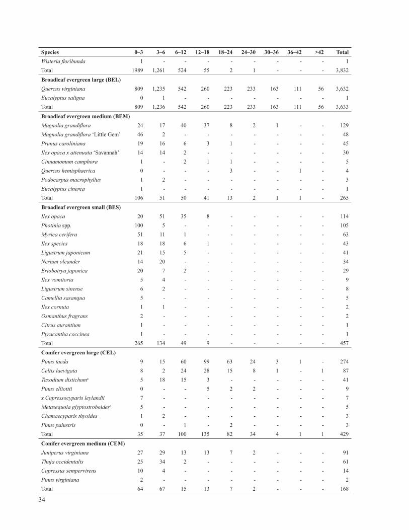
34

Species 0–3 3–6 6–12 12–18 18–24 24–30 30–36 36–42 >42 TotalWisteria fl oribunda 1 - - - - - - - - 1 Total 1989 1,261 524 55 2 1 - - - 3,832

Broadleaf evergreen large (BEL)Quercus virginiana 809 1,235 542 260 223 233 163 111 56 3,632 Eucalyptus saligna 0 1 - - - - - - - 1 Total 809 1,236 542 260 223 233 163 111 56 3,633

Broadleaf evergreen medium (BEM)Magnolia grandifl ora 24 17 40 37 8 2 1 - - 129 Magnolia grandifl ora ‘Little Gem’ 46 2 - - - - - - - 48 Prunus caroliniana 19 16 6 3 1 - - - - 45 Ilex opaca x attenuata ‘Savannah’ 14 14 2 - - - - - - 30 Cinnamomum camphora 1 - 2 1 1 - - - - 5 Quercus hemisphaerica 0 - - - 3 - - 1 - 4 Podocarpus macrophyllus 1 2 - - - - - - - 3 Eucalyptus cinerea 1 - - - - - - - - 1 Total 106 51 50 41 13 2 1 1 - 265

Broadleaf evergreen small (BES)Ilex opaca 20 51 35 8 - - - - - 114 Photinia spp. 100 5 - - - - - - - 105 Myrica cerifera 51 11 1 - - - - - - 63 Ilex species 18 18 6 1 - - - - - 43 Ligustrum japonicum 21 15 5 - - - - - - 41 Nerium oleander 14 20 - - - - - - - 34 Eriobotrya japonica 20 7 2 - - - - - - 29 Ilex vomitoria 5 4 - - - - - - - 9 Ligustrum sinense 6 2 - - - - - - - 8 Camellia sasanqua 5 - - - - - - - - 5 Ilex cornuta 1 1 - - - - - - - 2 Osmanthus fragrans 2 - - - - - - - - 2 Citrus aurantium 1 - - - - - - - - 1 Pyracantha coccinea 1 - - - - - - - - 1 Total 265 134 49 9 - - - - - 457

Conifer evergreen large (CEL)Pinus taeda 9 15 60 99 63 24 3 1 - 274 Celtis laevigata 8 2 24 28 15 8 1 - 1 87 Taxodium distichuma 5 18 15 3 - - - - - 41 Pinus elliottii 0 - - 5 2 2 - - - 9 x Cupressocyparis leylandii 7 - - - - - - - - 7 Metasequoia glyptostroboidesa 5 - - - - - - - - 5 Chamaecyparis thyoides 1 2 - - - - - - - 3 Pinus palustris 0 - 1 - 2 - - - - 3 Total 35 37 100 135 82 34 4 1 1 429

Conifer evergreen medium (CEM)Juniperus virginiana 27 29 13 13 7 2 - - - 91 Thuja occidentalis 25 34 2 - - - - - - 61 Cupressus sempervirens 10 4 - - - - - - - 14 Pinus virginiana 2 - - - - - - - - 2 Total 64 67 15 13 7 2 - - - 168

35

Species 0–3 3–6 6–12 12–18 18–24 24–30 30–36 36–42 >42 Total

Palm evergreen large (PEL)Phoenix canariensis 2 2 - - - - - - - 4 Total 2 2 - - - - - - - 4

Palm evergreen medium (PEM)Sabal palmetto 3 49 558 2,324 54 - - - - 2,988 Trachycarpus fortunei 2 4 2 - - - - - - 8 Total 5 53 560 2,324 54 - - - - 2,996

Palm evergreen small (PES)Butia capitata 4 11 39 92 74 3 - - - 223 Washingtonia robusta 2 5 - 5 - - - - - 12 Cycas revoluta 6 - 1 2 - - - - - 9 Yucca gloriosaa 1 - - - - - - - - 1 Total 13 16 40 99 74 3 - - - 245 Citywide total 3690 3,780 2,224 3,350 1,004 661 299 163 73 15,244

aTaxodium distichum and Metasequoia glyptostroboides are not evergreen trees, but have been grouped into this category as it most closely ap-proximates the level of benefi ts they provide. Yucca gloriosa is not actually a tree, but may grow large enough to provide the benefi ts of a tree and is categorized here in the most appropriate category.

36

Appendix B—Replacement Values

Species 0–3 3–6 6–12 12–18 18–24 24–30 30–36 36–42 >42 Total

Live oak 79,588 666,396 1,122,699 1,527,439 2,506,392 4,337,350 4,478,524 3,954,465 2,214,472 20,887,324

Crapemyrtle 172,835 542,299 820,276 243,048 20,260 - - - - 1,798,718

Sabal palmetto 60 1,203 21,117 132,186 4,177 - - - - 158,743

Water oak 1,739 8,860 82,594 596,516 2,069,399 2,521,279 911,086 156,486 3,844 6,351,803

Laurel oak 990 17,330 64,328 534,686 1,560,200 1,935,157 1,177,804 655,900 311,583 6,257,978

Flowering dogwood 15,256 65,368 163,810 33,025 - - - - - 277,459

Loblolly pine 1,130 7,602 115,127 476,936 560,072 341,236 70,205 28,696 - 1,601,002

Jelly palm 601 2,550 9,090 21,227 17,005 695 - - - 51,168

Red maple 4,922 48,022 22,728 23,355 39,905 - - - - 138,933

Chinese pistache 5,763 46,133 - - - - - - - 51,896

Muskogee crapemyrtle 8,920 23,364 11,429 - - - - - - 43,713

Southern magnolia 2,546 8,932 81,633 197,778 81,765 28,646 20,880 - - 422,181

London planetree 2,813 44,685 - - - - - - - 47,498

Honeylocust 2,033 11,789 83,220 53,581 - - - - - 150,622

Willow oak 466 32,814 57,744 36,291 60,207 69,266 85,363 31,184 34,859 408,193

American holly 2,200 27,350 70,068 42,673 - - - - - 142,291

Sweetgum 5,611 1,884 30,451 66,100 117,280 109,389 48,501 - - 379,215

October glory red maple 1,904 46,679 - - - - - - - 48,584

Photinia 10,962 2,694 - - - - - - - 13,656

Shumard oak 4,179 32,462 - - - - - - - 36,641

Eastern red cedar 4,182 13,559 22,428 50,349 56,124 22,379 - - - 169,022

Hackberry 946 1,151 40,066 113,370 116,366 77,825 24,703 - 25,788 400,215

Southern red oak - 28,126 - 9,284 76,474 88,053 118,907 146,040 30,882 497,767

Japanese zelkova 2,461 27,931 13,776 - - - - - - 44,168

American sycamore 1,580 10,869 16,083 22,060 52,277 122,693 47,031 143,397 24,121 440,111

Callery pear 4,248 13,201 15,822 42,064 7,388 - - - - 82,724

Tallowtree 3,184 8,412 20,086 19,184 - - - - - 50,866

Emerald Vase Chinese elm 6,822 12,470 - - - - - - - 19,292

Wax myrtle 5,379 5,795 1,905 - - - - - - 13,079

Rose-of-sharon 6,539 1,033 - - - - - - - 7,573

Northern white cedar 3,673 15,923 2,089 - - - - - - 21,685

Tuskegee crapemyrtle 2,426 14,986 - - - - - - - 17,411

Little gem southern magnolia 4,852 1,033 - - - - - - - 5,885

River birch 718 15,099 14,022 5,642 - - - - - 35,481

Carolina laurelcherry 3,182 7,266 7,945 10,903 5,863 - - - - 35,160

Holly 2,347 8,892 11,808 4,647 - - - - - 27,693

Pecan 377 2,022 13,530 53,103 87,753 47,837 21,682 28,696 - 255,000

Japanese privet 2,358 8,231 9,524 - - - - - - 20,113

Baldcypress 550 8,637 29,388 15,585 - - - - - 54,160

Ginkgo 1,305 10,008 7,626 - - - - - - 18,939

Oleander 1,477 10,335 - - - - - - - 11,811

Savannah holly 1,477 7,161 3,810 - - - - - - 12,447

Loquat tree 2,855 2,955 3,408 - - - - - - 9,218

Southern crabapple 1,527 4,662 3,188 3,513 - - - - - 12,890

Mimosa 1,722 4,076 3,479 - - - - - - 9,276

Tuscarora crapemyrtle 2,215 517 - - - - - - - 2,732

Chinese magnolia 2,023 2,057 1,476 - - - - - - 5,556

Siberian elm - - - 4,589 11,593 10,583 7,353 - - 34,118

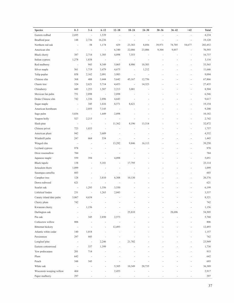
37

Species 0–3 3–6 6–12 12–18 18–24 24–30 30–36 36–42 >42 Total

Eastern redbud 2,695 - 1,539 - - - - - - 4,234

Bradford pear 148 2,736 16,236 - - - - - - 19,120

Northern red oak - 58 1,174 429 23,383 8,056 39,971 74,705 54,677 202,452

American elm - - - 6,340 22,086 23,006 9,304 9,857 - 70,593

Black cherry 387 2,714 1,385 4,898 7,353 - - - - 16,737

Italian cypress 1,278 1,838 - - - - - - - 3,116

Red mulberry - 943 8,349 5,065 8,906 10,303 - - - 33,565

Silver maple 561 1,719 3,479 4,675 - 1,212 - - - 11,646

Tulip poplar 858 2,162 2,091 3,983 - - - - - 9,094

Chinese elm 368 488 3,444 5,642 45,167 12,756 - - - 67,866

Chaste tree 324 2,621 5,714 4,453 - 14,323 - - - 27,435

Chinaberry 449 1,253 1,587 2,213 3,001 - - - - 8,504

Mexican fan palm 751 2,898 - 2,898 - - - - - 6,546

Drake Chinese elm 742 1,336 2,896 4,643 - - - - - 9,617

Sugar maple - 345 1,616 8,571 8,621 - - - - 19,154

American hornbeam - 2,055 7,145 - - - - - - 9,200

Sago palm 5,836 - 1,449 2,898 - - - - - 10,182

Yaupon holly 527 2,215 - - - - - - - 2,742

Slash pine - - - 11,362 8,196 13,314 - - - 32,872

Chinese privet 723 1,033 - - - - - - - 1,757

American plum 942 - 3,609 - - - - - - 4,552

Windmill palm 247 664 534 - - - - - - 1,445

Winged elm - - - 13,292 9,846 16,113 - - - 39,250

Leyland cypress 978 - - - - - - - - 978

Dixie rosemallow 784 - - - - - - - - 784

Japanese maple 559 394 - 4,098 - - - - - 5,051

Black tupelo 138 - 5,181 - 17,795 - - - - 23,114

Jerusalem thorn 1,099 - - - - - - - - 1,099

Sasanqua camellia 603 - - - - - - - - 603

Camphor tree 128 - 3,810 6,308 10,130 - - - - 20,376

Dawn redwood 621 - - - - - - - - 621

Scarlet oak - 1,293 1,356 3,550 - - - - - 6,199

Littleleaf linden 231 - 1,263 2,043 - - - - - 3,537

Canary island date palm 3,867 4,654 - - - - - - - 8,521

Cherry plum 742 - - - - - - - - 742

Kwanzan cherry - 1,156 - - - - - - - 1,156

Darlington oak - - - - 25,810 - - 28,696 - 54,505

Pin oak - 345 2,850 2,573 - - - - - 5,768

Corkscrew willow 806 - - - - - - - - 806

Bitternut hickory - - - 12,493 - - - - - 12,493

Atlantic white cedar 140 1,018 - - - - - - - 1,157

Persimmon 297 445 - - - - - - - 742

Longleaf pine - - 2,246 - 21,702 - - - - 23,949

Eastern cottonwood - 337 1,399 - - - - - - 1,736

Yew podocarpus 201 714 - - - - - - - 915

Plum 642 - - - - - - - - 642

Peach 348 345 - - - - - - - 693

White oak - - - 5,305 10,349 20,735 - - - 36,389

Wisconsin weeping willow 464 - - 2,453 - - - - - 2,917

Paper mulberry 297 - - - - - - - - 297

38

Species 0–3 3–6 6–12 12–18 18–24 24–30 30–36 36–42 >42 Total

Showy forsythia 211 - - - - - - - - 211

White ash 140 460 - - - - - - - 599

Chinese holly 90 517 - - - - - - - 607

Star magnolia 149 488 - - - - - - - 637

Sweet olive 289 - - - - - - - - 289

Virginia pine 360 - - - - - - - - 360

White poplar 213 - 915 - - - - - - 1,128

Sawtooth oak - 1,016 - - - - - - - 1,016

Post oak - - - 3,513 9,637 - - - - 13,150

Black oak - - - - 7,743 - - 28,696 - 36,439

Slippery elm - - - 7,289 - - - - - 7,289

Trident maple - - 1,539 - - - - - - 1,539

Amur maple 131 - - - - - - - - 131

Pignut hickory - - - 5,442 - - - - - 5,442

Sour orange 105 - - - - - - - - 105

Yellowwood - 388 - - - - - - - 388

Kousa dogwood 123 - - - - - - - - 123

Silver dollar eucalyptus 105 - - - - - - - - 105

Sydney blue gum - 517 - - - - - - - 517

Chinese parasoltree - - - 3,278 - - - - - 3,278

Black walnut - - - 4,643 - - - - - 4,643

Chinese fl ame tree 170 - - - - - - - - 170

Umbrella magnolia - - 1,241 - - - - - - 1,241

Fire thorn 217 - - - - - - - - 217

Swamp chestnut oak - - 1,722 - - - - - - 1,722

Black locust - - 717 - - - - - - 717

Black willow - 374 - - - - - - - 374

Christmasbush 105 - - - - - - - - 105

American basswood - - - - 4,098 - - - - 4,098

Black haw - 443 - - - - - - - 443

Japanese wisteria 239 - - - - - - - - 239

Moundlily yucca 25 - - - - - - - - 25

Citywide total 427,399 1,926,806 3,084,259 4,483,482 7,694,324 9,832,209 7,061,316 5,286,815 2,700,224 42,496,834

39

Appendix C—Methodology and Procedures

This analysis combines results of a citywide inven-tory with benefi t–cost modeling data to produce four types of information:

1. Resource structure (species composition, di-versity, age distribution, condition, etc.)

2. Resource function (magnitude of environmen-tal and aesthetic benefi ts)

3. Resource value (dollar value of benefi ts real-ized)

4. Resource management needs (sustainability, pruning, planting, and confl ict mitigation)

This Appendix describes street tree sampling, tree growth modeling, and the model inputs and calcu-lations used to derive the aforementioned outputs.

Growth Modeling

A stratifi ed random sample of street trees, drawn from Charleston’s municipal tree database, was in-ventoried to establish relations between tree age, size, leaf area and biomass; subsequently, estimates for determining the magnitude of annual benefi ts in relation to predicted tree size were derived. The sample was composed of the 19 most abundant species; from these data, growth of all street trees was inferred. The species were as follows:

• Live oak (Quercus virginiana)• Crapemyrtle (Lagerstroemia indica)• Sabal palmetto (Sabal palmetto)• Water oak (Quercus nigra)• Laurel oak (Quercus laurifolia)• Flowering dogwood (Cornus fl orida)• Loblolly pine (Pinus taeda)• Jelly palm (Butia capitata)• Red maple (Acer rubrum)• Southern magnolia (Magnolia grandifl ora)• Honeylocust (Gleditsia triacanthos)• Willow oak (Quercus phellos)• American holly (Ilex opaca)• Sweetgum (Liquidambar styracifl ua)• Hackberry (Celtis laevigata)

• Southern red oak (Quercus falcata)• American sycamore (Platanus occidentalis)• Callery pear (Pyrus calleryana)• Pecan (Carya illinoensis)

To obtain information spanning the life cycle of predominant tree species, the inventory was strati-fi ed into nine DBH classes:

• 0–3 in (0–7.62 cm)• 3–6 in (7.62–15.24 cm)• 6–12 in (15.24–30.48 cm• 12–18 in (30.48–45.72 cm)• 18–24 in (45.72–60.96 cm)• 24–30 in (60.96–76.2 cm)• 30–36 in (76.2–91.44)• 36–42 in (91.44–106.68 cm)• >42 in (>106.68 cm)

Thirty to seventy randomly selected trees of each species were selected to survey, along with an equal number of alternative trees. Tree measurements in-cluded DBH (to nearest 0.1 cm by sonar measuring device), tree crown and crown base (to nearest 0.5 m by altimeter), crown diameter in two directions (parallel and perpendicular to nearest street to near-est 0.5 m by sonar measuring device), tree condi-tion and location. Replacement trees were sampled when trees from the original sample population could not be located. Tree age was determined by street tree managers. Fieldwork was conducted in September 2004.

Crown volume and leaf area were estimated from computer processing of tree crown images ob-tained using a digital camera. The method has shown greater accuracy than other techniques (±25% of actual leaf area) in estimating crown vol-ume and leaf area of open-grown trees (Peper and McPherson 2003).

Linear regression was used to fi t predictive mod-els—with DBH as a function of age—for each of the 19 sampled species. Predictions of leaf surface area (LSA), crown diameter, and height metrics

40

were modeled as a function of DBH using best-fi t models (Peper et al. 2001).

Replacement Value

The monetary worth, or value, of a tree is based on people’s perception of it (Cullen 2000). There are several approaches that arborists use to develop a fair and reasonable perception of value (CTLA 1992, Watson 2002). The cost approach is widely used today and assumes that the cost of production equals value (Cullen 2002).

The trunk formula method (CTLA 1992), also called depreciated replacement cost, is a common-ly used approach for estimating tree value in terms of cost. It assumes that the benefi ts inherent in a tree are reproduced by replacing the tree, and there-fore, replacement cost is an indication of value. Re-placement cost is depreciated to refl ect differences in the benefi ts that would fl ow from an “idealized” replacement compared to the imperfect appraised tree.

We regard the terms “replacement value” and “re-placement cost” as synonymous indicators of the urban forest’s value. Replacement value is indi-cated by the cost of replacing existing trees with trees of similar size, species, and condition if all were destroyed, for example, by a catastrophic storm. Replacement cost should be distinguished from the value of annual benefi ts produced by the urban forest. The latter is a “snapshot” of benefi ts during one year, while the former accounts for the long-term investment in trees now refl ected in their number, stature, placement, and condition. Hence, the replacement value of a street tree population is many times greater than the value of annual ben-efi ts it produces.

The trunk formula method uses tree size, species, condition, and location factors to determine tree replacement value. Tree size is measured as trunk area (TA, cross-sectional area of the trunk based on DBH), while the other factors are assessed subjec-tively relative to a “high-quality” specimen and ex-pressed as percentages. The equation is

Replacement value = Basic value × Condition% × Location%

Basic value = Replacement cost + (Basic price × [TAA−TAR] × Species%)

where

Condition% = Rating of structural integrity and health; a higher percentage indicates better condi-tion (CTLA 1992).

Location% = Rating of the site itself (relative mar-ket value), contribution of the tree in terms of its aesthetic and functional attributes, and placement, which refl ects the effectiveness of realizing ben-efi ts; location is the sum of site, contribution, and placement divided by three (CTLA 1992). A higher percentage indicates better location.

Replacement cost = Sum of the cost of the replace-ment tree (of size TAR) and its installation .

Basic price = Cost of the largest available trans-plantable tree divided by TAR ($/in2).

TAA = Trunk area of appraised tree (in2) or height of clear trunk (linear ft) for palms.

TAR = Trunk area of replacement tree (in2) or height of clear trunk (linear ft) for palms.

Species% = Rating of the species’s longevity, main-tenance requirements, and adaptability to the local growing environment. (CTLA 1992).

In this study, data from the “Southeastern U.S. Tree Species Rating Guide” are used to calculate re-placement value (Smiley and Coder 2005). Species rating percentages are the midpoint for the ranges reported for zone 8. Street tree condition ratings are based on the inventory (or set at 70% when no data are available) and location ratings are arbitrarily set at 70%, indicative of a tree located along a typi-cal street. TAR is assumed to be 7.065 in2 for a 3” caliper tree; TAA is calculated using the midpoint for each DBH class. The basic price is $66/in2 TA. Replacement costs for trees are not specifi ed in the Southeastern Guide, so the replacement cost of $530 for a typical 3” caliper shade tree is adopted

41

from the Minnesota Supplement (Minnesota Soci-ety of Arboriculture 1996).

There were no palm data for the region, so basic prices ($/linear ft of clear trunk) and replacement costs ($/palm), which vary by species, are from the Western Chapter ISA Regional Supplement for the North Coast of California (WC-ISA 2004). TAR is assumed to be 15 linear ft; TAA is calculated as the midpoint for each palm height class.

Replacement values are calculated using the trunk formula equation for each species by DBH class, then summed across DBH classes and species to derive total replacement value for the population.

Identifying and Calculating Benefi ts

Annual benefi ts for Charleston’s municipal trees were estimated for the fi scal year 2004. Growth rate modeling information was used to perform com-puter-simulated growth of the existing tree popu-lation for one year and account for the associated annual benefi ts. This “snapshot” analysis assumed that no trees were added to, or removed from, the existing population during the year. (Calculations of CO2 released due to decomposition of wood from removed trees did consider average annual mortality.) This approach directly connects bene-fi ts with tree-size variables such as DBH and LSA. Many functional benefi ts of trees are related to pro-cesses that involve interactions between leaves and the atmosphere (e.g., interception, transpiration, photosynthesis); therefore, benefi ts increase as tree canopy cover and leaf surface area increase.

For each of the modeled benefi ts, an annual re-source unit was determined on a per-tree basis. Resource units are measured as MWh of electric-ity saved per tree; MBtu of natural gas conserved per tree; lbs of atmospheric CO2 reduced per tree; lbs of NO2, PM10, and VOCs reduced per tree; cu-bic feet of stormwater runoff reduced per tree; and square feet of leaf area added per tree to increase property values.

Prices were assigned to each resource unit (e.g., heating/cooling energy savings, air-pollution ab-

sorption, stormwater runoff reduction) using eco-nomic indicators of society’s willingness to pay for the environmental benefi ts trees provide.

Estimates of benefi ts are initial approximations as some benefi ts are diffi cult to quantify (e.g., impacts on psychological health, crime, and violence). In addition, limited knowledge about the physical processes at work and their interactions makes esti-mates imprecise (e.g., fate of air pollutants trapped by trees and then washed to the ground by rainfall). Therefore, this method of quantifi cation provides fi rst-order approximations. It is meant to be a gen-eral accounting of the benefi ts produced by urban trees—an accounting with an accepted degree of uncertainty that can, nonetheless, provide a sci-ence-based platform for decision-making.

Energy Savings

Buildings and paving, along with little tree canopy cover and soil cover, increase the ambient tem-peratures within a city. Research shows that even in temperate climate zones temperatures in urban centers are steadily increasing by approximately 0.5°F per decade. Winter benefi ts of this warming do not compensate for the detrimental effects of increased summertime temperatures. Because the electricity demand of cities increases about 1–2% per 1°F increase in temperature, approximately 3–8% of the current electric demand for cooling is used to compensate for this urban heat island effect (Akbari et al. 1992).

Warmer temperatures in cities have other implica-tions. Increases in CO2 emissions from fossil-fuel power plants, increased municipal water demand, unhealthy ozone levels, and human discomfort and disease are all symptoms associated with urban heat islands. In Charleston, there are opportunities to ameliorate the problems associated with hard-scape through strategic tree planting and steward-ship of existing trees thereby creating street and park landscapes that reduce stormwater runoff, conserve energy and water, sequester CO2, attract wildlife, and provide other aesthetic, social, and economic benefi ts.

42

For individual buildings, street trees can increase energy effi ciency in summer and increase or de-crease energy effi ciency in winter, depending on their location. During the summer, the sun is low in the eastern and western sky for several hours each day. Tree shade to protect east—and especially west—walls helps keep buildings cool. In the win-ter, allowing the sun to strike the southern side of buildings can warm interior spaces.

Trees reduce air movement into buildings and con-ductive heat loss from buildings. The rates at which outside air moves into a building can increase sub-stantially with wind speed. In cold, windy weather, the entire volume of air, even in newer or tightly sealed homes, may change every two to three hours. Trees can reduce wind speed and resulting air in-fi ltration by up to 50%, translating into potential annual heating savings of 25% (Heisler 1986). De-creasing wind speed reduces heat transfer through conductive materials as well. Cool winter winds, blowing against single-pane windows, can contrib-ute signifi cantly to the heating load of homes and buildings

Calculating Electricity and Natural Gas Benefi tsCalculations of annual building energy use per residential unit (unit energy consumption [UEC]) were based on computer simulations that incorpo-rated building, climate, and shading effects, fol-lowing methods outlined by McPherson and Simp-son (1999). Changes in UECs due to the effects of trees (ΔUECs) were calculated on a per-tree basis by comparing results before and after adding trees. Building characteristics (e.g., cooling and heating equipment saturations, fl oor area, number of sto-ries, insulation, window area, etc.) are differenti-ated by a building’s vintage, or age of construction: pre-1950, 1950 –1980, and post-1980. For example, all houses from 1950–1980 vintage are assumed to have the same fl oor area, and other construction characteristics. Shading effects for each of the 19 tree species were simulated at three tree-to-build-ing distances, for eight orientations and for nine tree sizes.

The shading coeffi cients of the trees in leaf (gaps in the crown as a percentage of total crown silhou-ette) were estimated using a photographic method that has been shown to produce good estimates (Wilkinson 1991). Crown areas were obtained us-ing the method of Peper and McPherson (2003) from digital photographs of trees from which back-ground features were digitally removed. Values for tree species that were not sampled, and leaf-off val-ues for use in calculating winter shade, were based on published values where available (McPherson 1984; Hammond et al. 1980). Where published values were not available, visual densities were as-signed based on taxonomic considerations (trees of the same genus were assigned the same value) or observed similarity to known species. Foliation periods for deciduous trees were obtained from the literature (McPherson 1984; Hammond et al. 1980) and adjusted for Charleston’s climate based on consultation with forestry supervisors (Burbage 2005).

Average energy savings per tree were calculated as a function of distance and direction using tree lo-cation distribution data specifi c to Charleston (i.e., frequency of trees located at different distances from buildings [setbacks] and tree orientation with respect to buildings). Setbacks were assigned to four distance classes: 0–20 ft, 20–40 ft, 40–60 ft and >60 ft. It was assumed that street trees within 60 ft of buildings provided direct shade on walls and windows. Savings per tree at each location were multiplied by tree distribution to determine location-weighted savings per tree for each species and DBH class, independent of location. Location-weighted savings per tree were multiplied by the number of trees of each species and DBH class and then summed to fi nd total savings for the city. Tree locations were based on the stratifi ed random sample conducted in summer 2004.

Land use (single-family residential, multifamily residential, commercial/industrial, other) for right-of-way trees was based on the same tree sample. A constant tree distribution was used for all land uses.

43

Three prototype buildings were used in the simula-tions to represent pre-1950, 1950–1980, and post-1980 construction practices (Ritschard et al. 1992). Building footprints were modeled as square, which was found to be refl ective of average impacts for a large number of buildings (Simpson 2002). Build-ings were simulated with 1.5-ft overhangs. Blinds had a visual density of 37%, and were assumed to be closed when the air conditioner was oper-ating. Thermostat settings were 78°F for cooling and 68°F for heating, with a 60°F night setback in winter. Unit energy consumptions were adjusted to account for equipment saturations (percentage of structures with different types of heating and cooling equipment such as central air conditioners, room air conditioners, and evaporative coolers) (Table C1).

Weather data for a typical meteorological year (TMY2) from Charleston were used (Renewable Resource Data Center 2005). Dollar values for en-ergy savings were based on electricity and natural gas prices of $0.09339/kWh and $1.19742/therm, respectively (SCANA 2005a, b).

Single-Family Residence AdjustmentsUnit energy consumptions for simulated single-family residences were adjusted for type and satu-ration of heating and cooling equipment, and for various factors (F) that modify the effects of shade and climate on heating and cooling loads:

ΔUECx=ΔUECshSFD × Fsh +ΔUECcl

SFD × Fcl Equation 1where

Fsh = Fequipment × APSF × Fadjacent shade × Fmultiple tree

Fcl = Fequipment × PCF

Fequipment = SatCAC + Satwindow × 0.25 + Satevap × (0.33 for cooling and 1.0 for heating).

Changes in energy use for higher density residen-tial and commercial structures were calculated from single-family residential results adjusted by average potential shade factors (APSF) and poten-tial climate factors (PCF); values were set to 1.0 for single-family residential buildings.

Total change in energy use for a particular land use was found by multiplying the change in UEC per tree by the number of trees (N):

Total change = N ×ΔUECx Equation 2

Subscript x refers to residential structures with 1, 2–4 or ≥5 units, SFD to simulated single-family detached structures, sh to shade, and cl to climate effects.

Estimated shade savings for all residential struc-tures were adjusted to account for shading of neighboring buildings and for overlapping shade from trees adjacent to one another. Homes adjacent to those with shade trees may benefi t from the trees on the neighboring properties. For example, 23% of the trees planted for the Sacramento Shade pro-gram shaded neighboring homes, resulting in an ad-ditional estimated energy savings equal to 15% of that found for program participants; this value was used here (Fadjacent shade = 1.15). In addition, shade from multiple trees may overlap, resulting in less building shade from an added tree than would re-sult if there were no existing trees. Simpson (2002) estimated that the fractional reductions in aver-age cooling and heating energy use were approxi-mately 6% and 5% percent per tree, respectively, for each tree added after the fi rst. Simpson (1998) also found an average of 2.5–3.4 existing trees per residence in Sacramento. A multiple tree reduction factor of 85% was used here, equivalent to approxi-mately three existing trees per residence.

In addition to localized shade effects, which were assumed to accrue only to street trees within 18–60 ft of buildings, lowered air temperatures and wind speeds due to neighborhood tree cover (referred to as climate effects) produce a net decrease in de-mand for summer cooling and winter heating. Re-duced wind speeds by themselves may increase or decrease cooling demand, depending on the circum-stances. To estimate climate effects on energy use, air-temperature and wind-speed reductions were estimated as a function of neighborhood canopy cover from published values following McPherson and Simpson (1999), then used as input for the

44

Sing

le fa

mily

de

tach

edM

obile

hom

esSi

ngle

-fam

ily a

ttac

hed

Mul

ti-fa

mily

2-4

uni

tsM

ulti-

fam

ily 5

+ un

itsC

omm

erci

al/

indu

stri

alIn

stit.

/Tr

ans-

port

a-tio

npr

e-19

5019

50-

1980

post

-19

80pr

e-19

5019

50-

1980

post

-19

80pr

e-19

5019

50-

1980

post

-19

80pr

e-19

5019

50-

1980

post

-19

80pr

e-19

5019

50-

1980

post

-19

80Sm

all

Lar

geC

oolin

g eq

uipm

ent f

acto

rsC

entra

l air/

heat

pum

p10

010

010

010

010

010

010

010

010

010

010

010

010

010

010

010

010

010

0

Evap

orat

ive

cool

er33

3333

3333

3333

3333

3333

3333

3333

3333

33

Wal

l/win

dow

uni

t25

2525

2525

2525

2525

2525

2525

2525

2525

25N

one

00

00

00

00

00

00

00

00

00

Coo

ling

satu

ratio

nsC

entra

l air/

heat

pum

p14

6376

1463

7614

6376

1463

7614

6376

8686

86

Evap

orat

ive

cool

er0

00

00

00

00

00

00

00

00

0

Wal

l/win

dow

uni

t59

235

5923

559

235

5923

559

235

99

9N

one

2714

190

00

00

00

00

00

05

55

Adj

uste

d co

olin

g sa

tura

tion

2869

7728

6977

2869

7728

6977

2869

7788

8888

Tabl

e C

1—Sa

tura

tion

adju

stm

ents

for c

oolin

g (%

).

45

building-energy-use simulations described earlier. Peak summer air temperatures were assumed to be reduced by 0.2°F for each percentage increase in canopy cover. Wind-speed reductions were based on the change in total tree plus building canopy cover resulting from the addition of the particular tree being simulated (Heisler 1990). A lot size of 10,000 ft2 was assumed.

Cooling and heating effects were reduced based on the type and saturation of air conditioning (Table C1) or heating (Table C2) equipment by vintage. Equipment factors of 33 and 25% were assigned to homes with evaporative coolers and room air condi-tioners, respectively. These factors were combined with equipment saturations to account for reduced energy use and savings compared to those simu-lated for homes with central air conditioning (Fequip-

ment). Building vintage distribution was combined with adjusted saturations to compute combined vintage/saturation factors for air conditioning (Ta-ble C3). Heating loads were converted to fuel use based on effi ciencies in Table C2. The “other” and “fuel oil” heating equipment types were assumed to be natural gas for the purpose of this analysis. Building vintage distributions were combined with adjusted saturations to compute combined vintage/saturation factors for natural gas and electric heat-ing (Table C3).

Multi-Family Residence Analysis

Unit energy consumptions (UECs) from single-fam-ily residential UECs were adjusted for multi-fam-ily residences (MFRs) to account for reduced shade resulting from common walls and multi-story con-struction. To do this, potential shade factors (PSFs) were calculated as ratios of exposed wall or roof (ceiling) surface area to total surface area, where total surface area includes common walls and ceil-ings between attached units in addition to exposed surfaces (Simpson 1998). A PSF of 1 indicates that all exterior walls and roofs are exposed and could be shaded by a tree, while a PSF of 0 indicates that no shading is possible (e.g., the common wall be-tween duplex units). Potential shade factors were estimated separately for walls and roofs for both

single- and multi-story structures. Average poten-tial shade factors were 0.74 for multi-family resi-dences of 2–4 units and 0.41 for ≥5 units.

Unit energy consumptions were also adjusted to account for the reduced sensitivity of multi-family buildings with common walls to outdoor tempera-ture changes. Since estimates for these PCFs were unavailable for multi-family structures, a multi-family PCF value of 0.80 was selected (less than single-family detached PCF of 1.0 and greater than small commercial PCF of 0.40; see next section).

Commercial and Other BuildingsReductions in unit energy consumptions for com-mercial/industrial (C/I) and industrial/transporta-tion (I/T) land uses due to the presence of trees were determined in a manner similar to that used for multi-family land uses. Potential shade factors of 0.40 were assumed for small C/I, and 0.0 for large C/I. No energy impacts were ascribed to large C/I structures since they are expected to have sur-face-to-volume ratios an order of magnitude larger than smaller buildings and less extensive window area. Average potential shade factors for I/T struc-tures were estimated to lie between these extremes; a value of 0.15 was used here. However, data re-lating I/T land use to building-space conditioning were not readily available, so no energy impacts were ascribed to I/T structures. A multiple-tree re-duction factor of 0.85 was used, and no benefi t was assigned for shading of buildings on adjacent lots.

Potential climate-effect factors of 0.40, 0.25 and 0.20 were used for small C/I, large C/I, and I/T, respectively. These values are based on estimates by Akbari (1992) and others who observed that commercial buildings are less sensitive to outdoor temperatures than houses.

The benefi cial effects of shade on UECs tend to in-crease with conditioned fl oor area (CFA) for typi-cal residential structures. As building surface area increases so does the area shaded. This occurs up to a certain point because the projected crown area of a mature tree (approximately 700–3,500 ft2) is often larger than the building surface areas being

46

Sing

le fa

mily

det

ache

dM

obile

hom

esSi

ngle

-fam

ily a

ttac

hed

Mul

ti-fa

mily

2-4

uni

tsM

ulti-

fam

ily 5

+ un

itsC

omm

erci

al/

indu

stri

alIn

stitu

tiona

l/Tr

ansp

orta

tion

pre-

1950

1950

-19

80po

st-

1980

pre-

1950

1950

-19

80po

st-

1980

pre-

1950

1950

-19

80po

st-

1980

pre-

1950

1950

-19

80po

st-

1980

pre-

1950

1950

-19

80po

st-

1980

Smal

lL

arge

Equi

pmen

t effi

cien

cies

AFU

E0.

750.

780.

780.

750.

780.

780.

750.

780.

780.

750.

780.

780.

750.

780.

780.

780.

780.

78

HSP

F6.

86.

88

6.8

6.8

86.

86.

88

6.8

6.8

86.

86.

88

88

8

HSP

F3.

412

3.41

23.

412

3.41

23.

412

3.41

23.

412

3.41

23.

412

3.41

23.

412

3.41

23.

412

3.41

23.

412

3.41

23.

412

3.41

2

Elec

tric

heat

satu

ratio

ns

Elec

tric

resi

stan

ce11

.516

.942

.111

.516

.942

.111

.516

.942

.111

.516

.942

.111

.516

.942

.14.

94.

94.

9

Hea

t pum

p6.

79.

924

.66.

79.

924

.66.

79.

924

.66.

79.

924

.66.

79.

924

.65.

45.

45.

4

Adj

uste

d el

ectri

c he

at sa

tura

tions

2.7

4.2

9.7

2.7

4.2

9.7

2.7

4.2

9.7

2.7

4.2

9.7

2.7

4.2

9.7

1.7

1.7

1.7

Nat

ural

gas

and

oth

er h

eatin

g sa

tura

tions

Nat

ural

gas

72.7

62.0

28.6

72.7

62.0

28.6

72.7

62.0

28.6

72.7

62.0

28.6

72.7

62.0

72.7

89.7

89.7

89.7

Oil

0.0

0.0

0.0

0.0

0.0

0.0

0.0

0.0

0.0

0.0

0.0

0.0

0.0

0.0

0.0

0.0

0.0

0.0

Oth

er9.

111

.34.

89.

111

.34.

89.

111

.34.

89.

111

.34.

89.

111

.34.

80

00

NG

hea

t sat

urat

ions

8273

3382

7333

8273

3382

7333

8273

3390

9090

Tabl

e C

2—Sa

tura

tion

adju

stm

ents

for h

eatin

g (%

, exc

ept A

FUE

[fra

ctio

n] a

nd H

SPF

[kBt

u/kW

h).

47

Sing

le fa

mily

de-

tach

edM

obile

hom

esSi

ngle

-fam

ily a

ttac

hed

Mul

ti-fa

mily

2-4

uni

tsM

ulti-

fam

ily 5

+ un

itsC

omm

erci

al/

indu

stri

alIn

stitu

tiona

l/Tr

ansp

orta

tion

pre-

1950

1950

-19

80po

st-

1980

pre-

1950

1950

-19

80po

st-

1980

pre-

1950

1950

-19

80po

st-

1980

pre-

1950

1950

-19

80po

st-

1980

pre-

1950

1950

-19

80po

st-

1980

Smal

lL

arge

Vin

tage

dis

tribu

tion

by b

uild

ing

type

26.9

39.6

33.6

26.9

39.6

33.6

26.9

39.6

33.6

26.9

39.6

33.6

26.9

39.6

33.6

100

100

100

Tree

dis

tribu

tion

by v

inta

ge a

nd b

uild

-in

g ty

pe

20.1

29.6

25.2

0.5

0.7

0.6

1.8

2.7

2.3

0.2

0.2

0.2

0.3

0.4

0.3

4.2

2.4

4.9

Com

bine

d vi

ntag

e, e

quip

men

t sat

urat

ion

fact

ors f

or c

oolin

g

Coo

ling

fact

or: s

hade

5.59

19.9

919

.04

0.13

0.47

0.45

0.45

1.61

1.53

0.03

0.11

0.11

0.03

0.10

0.10

1.3

0.4

0.0

Coo

ling

fact

or:

clim

ate

5.71

20.4

519

.48

0.13

0.46

0.44

0.42

1.51

1.44

0.02

0.07

0.07

0.03

0.12

0.11

1.1

2.2

0.0

Com

bine

d vi

ntag

e, e

quip

men

t sat

urat

ion

for h

eatin

g

Hea

ting

fact

or, n

atur

al

gas:

shad

e7.

9018

.96

23.2

91.

022.

463.

021.

002.

412.

960.

070.

170.

210.

130.

310.

381.

20.

40.

0

Hea

ting

fact

or, e

lec-

tric:

shad

e0.

541.

212.

390.

010.

030.

060.

040.

100.

190.

000.

010.

010.

000.

010.

010.

020.

010.

00

Hea

ting

fact

or, n

atur

al

gas:

clim

ate

16.4

621

.70

8.39

0.21

0.28

0.11

1.44

1.89

0.73

0.05

0.07

0.03

0.10

0.13

0.05

4.5

8.8

0.0

Hea

ting

fact

or, e

lec-

tric:

clim

ate

0.55

1.24

2.45

0.01

0.02

0.03

0.05

0.11

0.21

0.00

0.00

0.01

0.00

0.01

0.02

0.09

0.17

0.0

Tabl

e C

3—Bu

ildin

g vi

ntag

e di

stri

butio

n an

d co

mbi

ned

vint

age/

satu

ratio

n fa

ctor

s for

hea

ting

and

air c

ondi

tioni

ng.

48

shaded. A point is reached, however, at which no additional area is shaded as surface area increases. At this point, ΔUECs will tend to level off as CFA increases. Since information on the precise rela-tionships between change in UEC, CFA, and tree size is not available, it was conservatively assumed that ΔUECs in Equation 1 did not change for C/I and I/T land uses.

Atmospheric Carbon Dioxide Reduction

Sequestration (the net rate of CO2 storage in above- and below-ground biomass over the course of one growing season) is calculated for each species us-ing the tree-growth equations for DBH and height, described above, to calculate either tree volume or biomass. Equations from Pillsbury et al. (1998) are used when calculating volume. Fresh weight (kg/m3) and specifi c gravity ratios from Alden (1995, 1997) are then applied to convert volume to bio-mass. When volumetric equations for urban trees are unavailable, biomass equations derived from data collected in rural forests are applied (Tritton and Hornbeck 1982; Ter-Mikaelian and Korzukhin 1997).

Carbon dioxide released through decomposition of dead woody biomass varies with characteristics of the wood itself, the fate of the wood (e.g., amount left standing, chipped, or burned), and local soil and climatic conditions. Recycling of urban waste is now prevalent, and we assume here that most ma-terial is chipped and applied as landscape mulch. Calculations were conservative because they as-sumed that dead trees are removed and mulched in the year that death occurs, and that 80% of their stored carbon is released to the atmosphere as CO2 in the same year. Total annual decomposition is based on the number of trees in each species and age class that die in a given year and their biomass. Tree survival rate is the principal factor infl uencing decomposition. Tree mortality for Charleston was 1.0% per year for the fi rst fi ve years after plant-ing for street trees and 0.6% every year thereafter (Burbage 2005). Finally, CO2 released during tree maintenance was estimated to be 0.34 lb CO2 per inch DBH based on annual fuel consumption of

gasoline (~2,000 gal) and diesel fuel (~2,000 gal) (Burbage 2005).

Calculating Avoided CO2 Emissions Reducing building energy use reduces emissions of CO2. Emissions were calculated as the product of energy use and CO2 emission factors for electricity and heating. Heating fuel is largely natural gas and electricity in Charleston. The fuel mix for electri-cal generation included mainly coal (66.5%) and nuclear (32.9%) (U.S. EPA 2003).

Emissions factors for electricity (lb/MWh) and natural gas (lb/MBtu) fuel mixes are given in Ta-ble C4. The monetary value of avoided CO2 was $0.0075/lb based on average high and low esti-mates for emerging carbon trading markets (CO2e.com 2005).

Improving Air Quality

Calculating Avoided Emissions

Reductions in building energy use also result in reduced emissions of criteria air pollutants (those for which a national standard has been set by the EPA) from power plants and space-heating equip-ment. This analysis considered volatile organic hy-drocarbons (VOCs) and nitrogen dioxide (NO2)—both precursors of ozone (O3) formation—as well as sulfur dioxide (SO2) and particulate matter of <10 micron diameter (PM10). Changes in average annual emissions and their monetary values were calculated in the same way as for CO2, again us-ing utility specifi c emission factors for electricity and heating fuels (US EPA 2003). The prices of emissions savings were derived from models that calculate the marginal cost of controlling differ-ent pollutants to meet air quality standards (Wang and Santini 1995). Emissions concentrations were obtained from U.S. EPA (2005, Table C4), and population estimates from the US Census Bureau (2003).

Calculating Deposition and Interception

Trees also remove pollutants from the atmosphere. The hourly pollutant dry deposition per tree is ex-pressed as the product of the deposition velocity

49

Vd =1/(Ra+Rb+Rc), pollutant concentration (C), canopy projection (CP) area, and time step. Hourly deposition velocities for each pollutant were cal-culated using estimates for the resistances Ra, Rb, and Rc estimated for each hour over a year us-ing formulations described by Scott et al. (1998). Hourly concentrations for NO2, SO2, O3 and PM10 and hourly meteorological data (i.e., air tempera-ture, wind speed, solar radiation) for Charleston were obtained from the South Carolina Department of Environmental Quality (Shrenk 2004). The year 2003 was chosen because data were available and it closely approximated long-term, regional climate records.

Deposition was determined for deciduous species only when trees were in-leaf. A 50% re-suspension rate was applied to PM10 deposition. Methods de-scribed in the section “Calculating Avoided Emis-sions” were used to value emissions reductions; NO2 prices were used for ozone since ozone con-trol measures typically aim at reducing NO2.

Calculating BVOC Emissions Emissions of biogenic volatile organic carbon (sometimes called biogenic hydrocarbons or BVOCs) associated with increased ozone for-mation were estimated for the tree canopy using methods described by McPherson et al. (1998). In this approach, the hourly emissions of carbon in the form of isoprene and monoterpene are expressed as products of base emission factors and leaf bio-

mass factors adjusted for sunlight and temperature (isoprene) or simply temperature (monoterpene). Annual dry foliar biomass was derived from fi eld data collected in Charleston, SC during September 2004. The amount of foliar biomass present for each year of the simulated tree’s life was unique for each species. Hourly air temperature and solar radiation data for 2003 described in the pollutant uptake sec-tion were used as model inputs. Hourly emissions were summed to get annual totals (Table B4).

The ozone-reduction benefi t from lowering sum-mertime air temperatures, thereby reducing hy-drocarbon emissions from biogenic sources, was estimated as a function of canopy cover following McPherson and Simpson (1999). Peak summer air temperatures were reduced by 0.2°F for each per-centage increase in canopy cover. Hourly changes in air temperature were calculated by reducing this peak air temperature at every hour based on the hourly maximum and minimum temperature for that day, the maximum and minimum values of to-tal global solar radiation for the year. Simulation results from Los Angeles indicate that ozone reduc-tion benefi ts of tree planting with “low-emitting” species exceeded costs associated with their BVOC emissions (Taha 1996). This is a conservative ap-proach, since the benefi t associated with lowered summertime air temperatures and the resulting re-duced hydrocarbon emissions from anthropogenic sources were not accounted for.

Reducing Stormwater Runoff

The social benefi ts that result from reduced peak runoff include reduced property damage from fl ooding and reduced loss of soil and habitat due to erosion and sediment fl ow. Reduced runoff also results in improved water quality in streams, lakes, and rivers. This can translate into improved aquatic habitats, less human disease and illness due to con-tact with contaminated water and reduced storm-water treatment costs.

Calculating Stormwater Runoff ReductionsA numerical simulation model was used to estimate annual rainfall interception (Xiao et al. 1998). The

Emission factor Implied valuec ($/lb)

Electricity (lb/MWh)a

Natural gas (lb/MBtu)b

CO2 1,368 118.0 0.0075NO2 2.641 0.1020 1.04SO2 8.346 0.0006 1.28PM10 0.669 0.0075 0.76VOCs 0.668 0.0054 1.48

Table C4—Emissions factors and monetary implied val-ues for CO2 and criteria air pollutants.

aUSEPA 1998, eGRID 2002, except Ottinger et al. 1990 for VOCsbUSEPA 1998cCO2 from CO2e.com (2005), values for all other pollutants are based on methods of Wang and Santini (1995) using emissions concentra-tions from U.S. EPA (2005) and population estimates from the U.S. Census Bureau (2003).

50

interception model accounts for rainwater inter-cepted by the tree, as well as throughfall and stem fl ow. Intercepted water is stored on canopy leaf and bark surfaces. Once the storage capacity of the tree canopy is exceeded, rainwater temporarily stored on the tree surface will drip from the leaf surface and fl ow down the stem surface to the ground. Some of the stored water will evaporate. Tree can-opy parameters related to stormwater runoff reduc-tions include species, leaf and stem surface area, shade coeffi cient (visual density of the crown), tree height, crown diameter, and foliation period. Wind speeds were estimated for different heights above the ground; from this, rates of evaporation were es-timated.

The volume of water stored in the tree crown was calculated from crown-projection area (area under tree dripline), leaf area indices (LAI, the ratio of leaf surface area to crown projection area), and the depth of water captured by the canopy surface. Tree surface saturation was 0.04 in. Species-spe-cifi c shading coeffi cient, foliation period, and tree surface saturation storage capacity infl uence the amount of projected throughfall.

Hourly meteorological and rainfall data for 2003 at the Youmans Farm climate monitoring station (SCAN, site number: 2038, latitude: 32° 40’ N, lon-gitude: 81° 12’ W, elevation: 75 feet) in Hampton County, SC, were used in this simulation. The year 2003 was chosen because it most closely approxi-mated the 30-yr average rainfall of 52 in (1,320 mm). Annual precipitation at Youman’s Farm dur-ing 2003, however, was 61.2 in (1,554.7 mm); we made use of this data set because it was the most complete available. Storm events less than 0.2 in (5.1 mm) were assumed not to produce runoff and were dropped from the analysis. More complete descriptions of the interception model can be found in Xiao et al. (1998, 2000).

The social benefi ts that result from reduced peak runoff include reduced property damage from fl ooding and reduced loss of soil and habitat due to erosion and sediment fl ow. Reduced runoff also results in improved water quality in streams, lakes,

and rivers. This can translate into improved aquatic habitats, less human disease and illness due to con-tact with contaminated water and reduced storm-water treatment costs.

Charleston, SC assesses monthly stormwater fees to cover the costs of its stormwater management program. These fees were used as a proxy for the public’s willingness to pay for stormwater man-agement. Residential and commercial customers are charged monthly $4 per 2,200 ft2 of impervi-ous surface, which is $79.20 per acre of impervi-ous surface (McCrary 2005). The cost of control-ling runoff from a 10-year storm was used as the basis for valuing rainfall interception by trees in Charleston. This event was selected because most Best Management Practices (BMPs), such as reten-tion-detention basins, are designed to operate ef-fectively for storm events up to this size. Runoff from larger events are assumed to bypass BMPs, directly entering the system without pretreatment. Also, tree crown interception does not increase af-ter crowns are saturated, which usually occurs well before storm events reach this magnitude.

Runoff from 1 acre of impervious surface for a 10-year, 24-hour storm event (6.8 inches, South Carolina Department of Health and Environmental Control 2003) was 156,975 gals, assuming an aver-age runoff coeffi cient of 0.85. Assuming an annual stormwater management fee of $950.40 per acre of impervious surface, the resulting control cost is $0.00605 per gal.

Property Value and Other Benefi ts

Trees provide a host of aesthetic, social, economic, and health benefi ts that should be included in any benefi t–cost analysis. One of the most frequently cited reasons for planting trees is beautifi cation. Trees add color, texture, line, and form to the land-scape softening the hard geometry that dominates built environments. Research on the aesthetic qual-ity of residential streets has shown that street trees are the single strongest positive infl uence on scenic quality (Schroeder and Cannon 1983). Consumer surveys have shown that preference ratings in-

51

crease with the presence of trees in the commer-cial streetscape. In contrast to areas without trees, shoppers indicated that they shopped more often and longer in well-landscaped business districts, and were willing to pay more for goods and servic-es (Wolf 1999). Research in public-housing com-plexes found that outdoor spaces with trees were used signifi cantly more often than spaces without trees. By facilitating interactions among residents, trees can contribute to reduced levels of violence, as well as foster safer and more sociable neighbor-hood environments (Sullivan and Kuo 1996).

Well-maintained trees increase the “curb appeal” of properties. Research comparing sales prices of residential properties with different numbers and sizes of trees suggests that people are willing to pay 3–7% more for properties with ample trees versus few or no trees. One of the most compre-hensive studies on the infl uence of trees on resi-dential property values was based on actual sales prices and found that each large front-yard tree was associated with about a 1% increase in sales price (Anderson and Cordell 1988). Depending on aver-age home sale prices, the value of this benefi t can contribute signifi cantly to property tax revenues.

Scientifi c studies confi rm our intuition that trees in cities provide social and psychological benefi ts. Humans derive substantial pleasure from trees, whether it is inspiration from their beauty, a spiri-tual connection, or a sense of meaning (Dwyer et al. 1992; Lewis 1996). Following natural disasters, people often report a sense of loss if the urban for-est in their community has been damaged (Hull 1992). Views of trees and nature from homes and offi ces provide restorative experiences that ease mental fatigue and help people to concentrate (Ka-plan and Kaplan 1989). Desk-workers with a view of nature report lower rates of sickness and greater satisfaction with their jobs compared to those hav-ing no visual connection to nature (Kaplan 1992). Trees provide important settings for recreation and relaxation in and near cities. The act of planting trees can have social value, for community bonds between people and local groups often result.

The presence of trees in cities provides public health benefi ts and improves the well being of those who live, work and play in cities. Physical and emotional stress has both short-term and long-term effects. Prolonged stress can compromise the human immune system. A series of studies on hu-man stress caused by general urban conditions and city driving showed that views of nature reduce the stress response of both body and mind (Parsons et al. 1998). City nature also appears to have an “im-munization effect,” in that people show less stress response if they have had a recent view of trees and vegetation. Hospitalized patients with views of nature and time spent outdoors need less medi-cation, sleep better, have a better outlook, and re-cover quicker than patients without connections to nature (Ulrich 1985). Trees reduce exposure to ul-traviolet light, thereby lowering the risk of harmful effects from skin cancer and cataracts (Tretheway and Manthe 1999).

Certain environmental benefi ts from trees are more diffi cult to quantify than those previously described, but can be just as important. Noise can reach unhealthy levels in cities. Trucks, trains, and planes can produce noise that exceeds 100 decibels, twice the level at which noise becomes a health risk. Thick strips of vegetation in conjunction with landforms or solid barriers can reduce highway noise by 6–15 decibels. Plants absorb more high frequency noise than low frequency, which is ad-vantageous to humans since higher frequencies are most distressing to people (Miller 1997).

Urban forests can be oases, sometimes containing more vegetative diversity than surrounding rural areas. Numerous types of wildlife inhabit cities and are generally highly valued by residents. For ex-ample, older parks, cemeteries, and botanical gar-dens often contain a rich assemblage of wildlife. Street-tree corridors can connect a city to surround-ing wetlands, parks, and other greenspace resourc-es that provide habitats that conserve biodiversity (Platt et al.1994).

Urban and community forestry can provide jobs for both skilled and unskilled labor. Public service

52

programs and grassroots-led urban and community forestry programs provide horticultural training to volunteers across the United States. Also, urban and community forestry provides educational opportu-nities for residents who want to learn about nature through fi rst-hand experience (McPherson and Mathis 1999). Local nonprofi t tree groups, along with municipal volunteer programs, often provide educational materials, work with area schools, and offer hands-on training in the care of trees.

Calculating Changes in Property Values and Other Benefi ts In an Athens, GA, study (Anderson and Cordell 1988), a large front-yard tree was found to be as-sociated with a 0.88% increase in average home resale values. In our study, the annual increase in leaf surface area of a typical mature large tree (25-year-old live oak, average leaf surface area 2,758 ft2) was the basis for valuing the capacity of trees to increase property value.

Assuming the 0.88% increase in property value held true for the city of Charleston, each large tree would be worth $1,615 based on the 3rd quarter, 2005, average single-family-home resale price in Charleston ($183,500) (National Association of Re-altors 2005). However, not all trees are as effective as front-yard trees in increasing property values. For example, trees adjacent to multifamily hous-ing units will not increase the property value at the same rate as trees in front of single-family homes. Therefore, a citywide street tree reduction factor (0.935) was applied to prorate trees’ value based on the assumption that trees adjacent to different land-uses make different contributions to property sales prices. For this analysis, the street reduction factor refl ects the distribution of street trees in Charleston by land-use. Reduction factors were single-home residential (100%), multi-home residential (70%), small commercial (66%), industrial/institutional/large commercial (40%), park/vacant/other (40%) (Gonzales 2004, McPherson et al. 2001).

Given these assumptions, a typical large street tree was estimated to increase property values by $0.34/ft2 of LSA. For example, it was estimated that a

single, street-side live oak added about 212 ft2 of LSA per year when growing in the DBH range of 12–18 in. Therefore, during this period of growth, live oak trees effectively added $72.21, annually, to the value of an adjacent home, condominium, or business property (212 ft2x $0.34/ft2 = $72.21).

Estimating Magnitude of Benefi ts

Resource units describe the absolute value of the benefi ts of Charleston’s street trees on a per-tree basis. They include kWh of electricity saved per tree, kBtu of natural gas conserved per tree, lbs of atmospheric CO2 reduced per tree, lbs of NO2, PM10, and VOCs reduced per tree, cubic feet of stormwater runoff reduced per tree, and square feet of leaf area added per tree to increase property val-ues. A dollar value was assigned to each resource unit based on local costs.

Estimating the magnitude of the resource units produced by all street and park trees in Charleston required four steps: (1) categorizing street trees by species and DBH based on the city’s street-tree in-ventory, (2) matching other signifi cant species with those that were modeled, (3) grouping remaining “other” trees by type, and (4) applying resource units to each tree.

Categorizing Trees by DBH Class

The fi rst step in accomplishing this task involved categorizing the total number of street trees by rel-ative age (as a function of DBH class). The inven-tory was used to group trees into the DBH classes described at the beginning of this chapter.

Next, the median value for each DBH class was determined and subsequently used as a single value to represent all trees in each class. For each DBH value and species, resource units were estimated using linear interpolation.

Applying Resource Units to Each Tree

The interpolated resource-unit values were used to calculate the total magnitude of benefi ts for each DBH class and species. For example, assume that there are 300 red maples citywide in the 30–36 in

53

DBH class. The interpolated electricity and natural gas resource unit values for the class midpoint (33 in) were 283.4 kWh and 665 kBtu per tree, respec-tively. Therefore, multiplying the resource units for the class by 300 trees equals the magnitude of an-nual heating and cooling benefi ts produced by this segment of the population: 85,020 kWh of electric-ity saved and 199,500 kBtu of natural gas saved.

Matching Signifi cant Species with Modeled Species

To extrapolate from the 19 municipal species mod-eled for growth to the entire inventoried tree popu-lation, each species representing over 1% of the population was matched with the modeled species that it most closely resembled. Less abundant spe-cies that were not matched were then grouped into the “Other” categories described below.

Grouping Remaining “Other” Trees by Type

The species that were less than 1% of the popula-tion were labeled “other” and were categorized ac-cording into classes based on tree type (one of four life forms and three mature sizes):

• Broadleaf deciduous: large (BDL), medi-um (BDM), and small (BDS).

• Broadleaf evergreen: large (BEL), medium (BEM), and small (BES).

• Coniferous evergreen: large (CEL), me-dium (CEM), and small (CES).

• Palm: large (PEL), medium (PEM), and small (PES).

Large, medium, and small trees were >40 ft, 25–40 ft, and <25 ft in mature height, respectively. A typi-cal tree was chosen to represent each of the above 15 categories to obtain growth curves for “other” trees falling into each of the categories:

BDL Other = Pecan (Carya illinoensis)BDM Other = Pear (Pyrus calleryana)BDS Other = Crapemyrtle (Lagerstroemia indica)BEL Other = Live oak (Quercus virginiana)

BEM Other = Southern magnolia (Magnolia gran-difl ora)BES Other = American holly (Ilex opaca)CEL Other = Loblolly pine (Pinus taeda) CEM Other = Eastern red cedar (Juniperus virgin-iana)CES Other = Bolander beach pine (Pinus con-torta)PEL Other = Canary Island date palm (Phoenix canariensis)PEM Other = Sabal palmetto (Sabal palmetto)PES Other = Jelly palm (Butia capitata)

When local data were not measured for certain categories (e.g., CES, PEL), growth data from similar-sized species in a different region were used.

Calculating Net Benefi ts And Benefi t–Cost Ratio

It is impossible to quantify all the benefi ts and costs produced by trees. For example, owners of property with large street trees can receive bene-fi ts from increased property values, but they may also benefi t directly from improved health (e.g., reduced exposure to cancer-causing UV radiation) and greater psychological well-being through visu-al and direct contact with trees. On the cost side, in-creased health-care costs may be incurred because of nearby trees, due to allergies and respiratory ail-ments related to pollen. The values of many of these benefi ts and costs are diffi cult to determine. We assume that some of these intangible benefi ts and costs are refl ected in what we term “property value and other benefi ts.” Other types of benefi ts we can only describe, such as the social, educational, and employment/training benefi ts associated with the city’s street tree resource. To some extent connect-ing people with their city trees reduces costs for health care, welfare, crime prevention, and other social service programs.

Charleston residents can obtain additional econom-ic benefi ts from street trees depending on tree loca-tion and condition. For example, street trees can provide energy savings by lowering wind veloci-

54

ties and subsequent building infi ltration, thereby reducing heating costs. This benefi t can extend to the neighborhood, as the aggregate effect of many street trees reduces wind speed and reduces city-wide winter energy use. Neighborhood property values can be infl uenced by the extent of tree can-opy cover on streets. The community benefi ts from cleaner air and water. Reductions in atmospheric CO2 concentrations due to trees can have global benefi ts.

Net Benefi ts and Costs Methodology

To assess the total value of annual benefi ts (B) for each park and street tree (i) in each management area (j) benefi ts were summed:

Equation 3

where

e = price of net annual energy savings = annual natural gas savings + annual electricity savings

a = price of annual net air quality improvement = PM10 interception + NO2 and O3 absorption + avoided power plant emissions – BVOC emis-sions

c = price of annual carbon dioxide reductions = CO2 sequestered – releases + CO2 avoided from reduced energy use

h = price of annual stormwater runoff reductions = effective rainfall interception

p = price of aesthetics = annual increase in property value

Total net expenditures were calculated based on all identifi able internal and external costs associated with the annual management of municipal trees citywide (Koch 2004). Annual costs for the mu-nicipality (C) were summed:

C = p + t + r + d + e + s + c + l + a + q

p = annual planting expenditure

t = annual pruning expenditure

r = annual tree and stump removal and dis-posal expenditure

d = annual pest and disease control expenditure

e = annual establishment/irrigation expenditure

s = annual price of repair/mitigation of infra-structure damage

c = annual price of litter/storm clean-up

l = average annual litigation and settlements expenditures due to tree-related claims

a = annual expenditure for program adminis-tration

q = annual expenditures for inspection/answer service requests

Total citywide annual net benefi ts as well as the benefi t–cost ratio (BCR) were calculated using the sums of benefi ts and costs:

Citywide Net Benefi ts = B – C Equation 4

BCR = B – C Equation 5

( )⎥⎦

⎤⎢⎣

⎡++++= ∑∑ ijijijijij

nn

phcaeijB11

55

References

Akbari, H.; Davis, S.; Dorsano, S.; Huang, J.; Winnett, S., eds. 1992. Cooling Our Communities: A Guidebook on Tree Planting and Light-Colored Surfacing. Washington, DC: U.S. Environmental Protection Agency.; 26 p.

Alden, H.A. 1995. Hardwoods of North America. USDA For-est Service, FPL General Technical Report No. 83. Madison, WI. 136 p.

Alden, H.A. 1997. Softwoods of North America. USDA Forest Service, FPL General Technical Report No. 102. Madison, WI. 151 p.

American Forests. 2005. Urban Ecosystem Analysis, Mecklen-burg County, North Carolina. Calculating the Value of Nature. American Forests, Washington, D.C.

Anderson, L.M. and H.K. Cordell. 1988. Residential property values improve by landscaping with trees. Southern Jour-nal of Applied Forestry 9:162-166.

Bankrate.com. 2004. Home values make unprecedented leap. Accessed via the World Wide Web <http://www.bankrate.com/brm/news/real-estate/home-values2.asp#NC> on Octo-ber 1, 2004.

Benjamin, M.T. and A.M. Winer. 1998. Estimating the ozone-forming potential of urban trees and shrubs. Atmos. En-viron., 32: 53-68.

Burbage, D. 2005. Personal communication. Urban Forestry Su-perintendent, City of Charleston, SC.

Chandler, T.J. 1965. The Climate of London. London, Hutchin-son.

Clark, J.R., N.P. Matheny, G. Cross and V. Wake. 1997. A model of urban forest sustainability. J. Arboric. 23(1):17-30.

CO2e.com. 2005. Market Size and Pricing. Accessed via the World Wide Web <http://www.co2e.com/stratagies/Addi-tionalInfo.asp?PageID=273#1613> on September 8, 2005.

CTLA (Council of Landscape & Tree Appraisers). 1992. Guide for Plant Appraisal (8th ed.). International Society of Ar-boriculture, Champaign, IL. 103p.

Costello, L. and Jones, K. 2003. Reducing Infrastructure Dam-age by Tree Roots: A Compendium of Strategies. Western Chapter International Society of Arboriculture, Cohasset, CA.

Cullen, S. 2000. Tree appraisal: What is the trunk formula method (9th edn.)? Arboric. Consult. 30(5):3.

Cullen, S. 2002. Tree appraisal: Can depreciation factors be rated greater than 100%? J. Arbor. 28(3):153-158.

Davey Resource Group. 2000. Urban Forestry Management Plan for the City of Charleston, South Carolina. Davey Resource Group, Kent, OH.

Duryea, M.L. 1997. Wind and trees: surveys of tree damage in the Florida Panhandle after Hurricanes Erin and Opal.

Circular 1183, Florida Cooperative Extension Service. Uni-versity of Florida, Gainesville.

Duryea, M.L.; Blakeslee, W.G.; Vasquez, R.A. 1996. Wind and trees: a survey of homeowners after Hurricane Andrew. J. Arboric 22:44–50.

Dwyer, J.F., E.G. McPherson, H.W. Schroeder and R.A. Rown-tree. 1992. Assessing the benefi ts and costs of the urban forest. J. Arboric 18(5):227-234.

Forschler, B.T. 2002. The Formosan Subterranean Termite. Ac-cessed via the World Wide Web http://www.gaipm.org/fact-sheets/formosan.html on April 26, 2002.

Gonzalez, S. 2004. Personal communication on September 23, 2004 re Landscape Assessment Districts method of appor-tionment. Landscape Maintenance Manager, Vallejo, CA.

Hammond J., J. Zanetto and C. Adams. 1980. Planning Solar Neighborhoods. California Energy Commission.

Heisler, G.M. 1986. Energy savings with trees. J. Arboric. 12(5):113-125.

Heisler, G. M. 1990. Mean wind speed below building height in residential neighborhoods with different tree densities. ASHRAE Transactions 96:1:1389-1396.

Hull, R.B. 1992. How the public values urban forests. J. Arbo-ric. 18(2):98-101.

Kaplan, R. 1992. Urban Forestry and the Workplace. In P.H. Gobster (Ed). Managing Urban and High-Use Recreation Settings. USDA Forest Service, General Technical Report NC-163. Chicago, IL: North Central Forest Experimentation Center.

Kaplan, R. and S. Kaplan. 1989. The Experience of Nature: A Psychological Perspective. Cambridge University Press, Cambridge, UK.

Lewis, C.A. 1996. Green Nature/Human Nature: The Meaning of Plants in Our Lives. University of Illinois Press, Chi-cago, IL.

Maco, S.E. and E.G. McPherson. 2002. Assessing canopy cover over streets and sidewalks in street tree populations. J. Arboric. 28(6):270-276.

Maco, S.E. and E.G. McPherson. 2003. A practical approach to assessing structure, function, and value of street tree pop-ulations in small communities. J. Arboric. 29(2):84-97.

McPherson, E. G. 1984. Planting design for solar control, chap-ter 8. In: Energy Conserving Site Design, Am. Soc. Land-scape Archit., Washington, D.C. p.141-164.

McPherson, E.G. 1993. Evaluating the cost effectiveness of shade trees for demand-side management. The Electricity Journal 6(9): 57-65.

56

McPherson, E.G. and S. Mathis (Eds.) 1999. Proceedings of the Best of the West Summit. Western Chapter, International Society of Arboriculture: Sacramento, CA: 93 p.

McPherson, E.G. and R.A. Rowntree. 1989. Using structural measures to compare twenty-two U.S. street tree popula-tions. Landscape Journal 8:13-23.

McPherson, E.G. and J.R. Simpson. 1999. Guidelines for Cal-culating Carbon Dioxide Reductions Through Urban Forestry Programs. USDA Forest Service, PSW General Technical Report No. 171, Albany, CA.

McPherson, E.G. and J.R. Simpson. 2002. A comparison of municipal forest benefi ts and costs in Modesto and Santa Monica, California, USA. Urban For. Urban Green. 1(2002):61-74.

McPherson, E.G. and Q. Xiao. 2004. A Storm Runoff Model for the Trust for Public Land’s “What is a Park Worth?” Project. Center for Urban Forest Research, USDA Forest Service, Pacifi c Southwest Research Station 12 pp.

McPherson, E.G.; Simpson, J.R.; Peper, P.J.; Xiao, Q. 1999b. Benefi t-cost analysis of Modesto’s municipal urban for-est. J. Arboric. 25(5):235–248.

McPherson, E.G.; Simpson, J.R.; Peper, P.J.; Xiao, Q. 2001. Tree Guidelines for Inland Empire Communities. Western Cen-ter for Urban Forest Research and Education, USDA Forest Service: Davis, CA.

McPherson, E.G., J.R. Simpson, Q. Xiao, P.J. Peper, S.E. Maco. 2003. Benefi t–Cost Analysis of Fort Collins’ Municipal Forest. Center for Urban Forest Research, USDA Forest Service, Pacifi c Southwest Research Station.

McPherson, E.G.; Simpson, J.R.; Peper, P.J.; Gardner, S.L.; Var-gas, K.E.; Ho, J.; Maco, S.; Xiao, Q. 2004a. City of Bis-marck, North Dakota, Street Tree Resource Analysis. Internal Tech. Rep. Davis, CA: U.S. Department of Agricul-ture, Forest Service.

McPherson, E.G.; Simpson, J.R.; Peper, P.J.; Gardner, S.L.; Var-gas, K.E.; Ho, J.; Maco, S.; Xiao, Q. 2004b. City of Chey-enne, Wyoming, Municipal Tree Resource Analysis. Inter-nal Tech. Rep. Davis, CA: U.S. Department of Agriculture, Forest Service.

McPherson, E.G., J.R. Simpson, P.J. Peper, S.E. Maco, Q. Xiao. 2005a. Municipal forest benefi ts and costs in fi ve U.S. cit-ies. Journal of Forestry 103(8):411–416.

McPherson, E.G.; Simpson, J.R.; Peper, P.J.; Gardner, S.L.; Var-gas, K.E.; Ho, J.; Maco, S.; Xiao, Q. 2005b. City of Char-lotte, North Carolina, Municipal Forest Resource Analy-sis. Internal Tech. Rep. Davis, CA: U.S. Department of Agri-culture, Forest Service.

McPherson, E.G.; Simpson, J.R.; Peper, P.J.; Maco, S.; Xiao, Q. 2005c. City of Glendale, AZ, Municipal Forest Resource Analysis. Internal Tech. Rep. Davis, CA: U.S. Department of Agriculture, Forest Service.

McPherson, E.G.; Simpson, J.R.; Peper, P.J.; Maco, S.; Gardner, S.L.; Cozad, S.K.; Xiao, Q. 2005d. City of Minneapolis,

MN, Municipal Tree Resource Analysis. Internal Tech. Rep. Davis, CA: U.S. Department of Agriculture, Forest Service.

McPherson, E.G.; Simpson, J.R.; Peper, P.J.; Gardner, S.L.; Var-gas, K.E.; Ho, J.; Xiao, Q. 2005e. City of Boulder, Colora-do, Municipal Tree Resource Analysis. Internal Tech. Rep. Davis, CA: U.S. Department of Agriculture, Forest Service.

Maco, S.E.; McPherson, E.G.; Simpson, J.R.; Peper, P.J.; Xiao, Q. 2005f. City of Berkeley, California, Municipal Tree Resource Analysis. Internal Tech. Rep. Davis, CA: U.S. De-partment of Agriculture, Forest Service.

Miller, R.W. 1997. Urban forestry: planning and managing urban greenspaces. 2nd. ed. Upper Saddle River: Prentice-Hall; 502 p.

Minnesota Society of Arboriculture. 1996. Minnesota Supple-ment to the Guide for Plant Appraisal. Minnesota Society of Arboriculture, Saint Paul, MN.

Moll, G. and C. Kollin. 1993. A new way to see our city forests. American Forests 99(9-10):29-31.

National Association of Realtors. 2005. Accessed via the World Wide Web <http http://www.realtor.org/Research.nsf/fi les/REL05Q3T.pdf/> February 2005.

Ottinger, R.L.; Wooley, D.R.; Robinson, N.A.; Hodas, D.R.; Babb, S.E. 1990. Environmental Costs of Electricity. Pace University Center for Environmental Legal Studies, Oceana Publications, Inc. New York.

Parsons, R., L.G. Tassinary, R.S. Ulrich, M.R. Hebl and M. Gross-man-Alexander. 1998. The view from the road: implica-tions for stress recovery and immunization. Journal of Environmental Psychology 18(2):113-140.

Peper, P.J. and E.G. McPherson. 2003. Evaluation of four meth-ods for estimating leaf area of isolated trees. Urban For-estry and Urban Greening 2:19-30.

Peper, P.J., E.G. McPherson and S.M. Mori. 2003. Equations for predicting diameter, height, crown width, and leaf area of San Joaquin Valley street trees. Journal of Arboriculture (27(6):306-317.

Piedmont Natural Gas 2004. Accessed via the World Wide Web <http://www.piedmontng.com/rates/ratesNC?pageId=092004NC.htm&section=res> June 2005.

Pillsbury, N.H.; Reimer, J.L.; Thompson R.P. 1998. Tree Volume Equations for Fifteen Urban Species in California. Tech. Rpt. 7. Urban Forest Ecosystems Institute, California Poly-technic State University; San Luis Obispo, CA. 56 p.

Platt, R.H., R.A Rowntree and P.C. Muick, eds. 1994. The Eco-logical City. Boston, MA, Univ. of Massachusetts. 292 p.

Renewable Resource Data Center. 2005. National Solar Radia-tion Data Base Typical Year Data. Accessed via the World Wide Web <http://rredc.nrel.gov/solar/old_data/nsrdb/tmy2/> November 2004.

Richards, N.A. 1982/83. Diversity and stability in a street tree population. Urban Ecology 7: 159-171.

57

Ritschard, R.L., J.W. Hanford and A.O. Sezgen. 1992. Single-family heating and cooling requirements: assumptions, methods, and summary results. Publication GRI-91/0236. Chicago: Gas Research Institute; 97 p.

SCANA Corporation. 2005a. Accessed via the World Wide Web at http://www.scana.com/SCEG/At+Home/Customer+Service/Rates/Residential+Electric+Rates.htm on 11 April 2005.

SCANA Corporation. 2005b. Accessed via the World Wide Web at <http://www.scana.com/SCEG/At+Home/Customer+Service/Rates/Residential+Gas+Rates.htm> on 11 April 2005.

Schroeder, H.W. and W.N. Cannon. 1983. The esthetic contribu-tion of trees to residential streets in Ohio towns. Journal of Arboriculture. 9: 237-243.

Scott, K.I., E.G. McPherson, and J.R. Simpson. 1998. Air pol-lutant uptake by Sacramento’s urban forest. Journal of Arboriculture 24(4):224-234.

Shrenk, J. 2004. Personal communication, SC Department of En-vironmental Quality, 8 October 2004.

Simpson, J.R. 1998. Urban forest impacts on regional space conditioning energy use: Sacramento County case study. Journal of Arboriculture 24(4): 201-214.

Simpson, J.R. 2002. Improved estimates of tree shade effects on residential energy use. Energy and Buildings 34(10): 173-182.

South Carolina Department of Health and Environmental Control. 2003. South Carolina stormwater management and sediment control handbook for land disturbance activities. Accessed on the World Wide Web at <http://www.scdhec.net/eqc/wa-ter/pubs/swmanual.pdf>.

Smiley E.T. and K. Coder. 2005. Southeastern United States Tree Species Rating Guide. Southern Chapter, International Society of Arboriculture, Mount Airy, NC.

Sullivan, W.C. and E.E. Kuo. 1996. Do trees strengthen urban communities, reduce domestic violence? Arborist News. 5(2):33-34.

Ter-Mikaelian, M.T. and M.D. Korzukhin. 1997. Biomass equa-tions for sixty-fi ve North American tree species. For Ecol and Management 97: 1-24.

Thompson, R.P. and J.J. Ahern. 2000. The State of Urban and Community Forestry in California: Status in 1997 and Trends since 1988. California Dept. of Forestry and Fire Protection, Technical Report No. 9. Urban Forest Ecosys-tems Institute, Cal Poly State University, San Luis Obispo, CA. pp. 48.

Touliatos, P. and E. Roth. 1971. Hurricanes and trees: ten les-sons from Camille. J. For. 69:285–289.

Tretheway, R. and A. Manthe. 1999. Skin cancer prevention: another good reason to plant trees. In McPherson, E.G. and Mathis, S. Proceedings of the Best of the West Summit. University of California, Davis, CA.

Tritton, L.M. and J.W. Hornbeck. 1982. Biomass Equations for Major Tree Species of the Northeast. USDA Forest Ser-vice, NE General Technical Report No. 69. Broomall, PA. 46 p.

U.S. Census Bureau. 2003. 2003 Population Estimates, Census 2000, 1990. Accessed via the World Wide Web <http://www.census.gov/population/cen2000/phc-t29/tab06.pdf> on Au-gust 18, 2005.

U.S. Environmental Protection Agency. 1998. Ap-42 Compila-tion of Air Pollutant Emission Factors (5th Edition). Vol-ume I. Research Triangle Park, NC.

U.S. Environmental Protection Agency. 2003. E-GRID (E-GRID2002 Edition).

U.S. Environmental Protection Agency. 2004. Monitor Values Report for Anoka and Hennepin Co, MN. Accessed via the World Wide Web <http://www.epa.gov/air/data/reports.html> on Sept 12, 2004.

Ulrich, R. S. 1985. Human responses to vegetation and land-scapes. Landscape and Urban Planning 13: 29-44.

Wang, M.Q.; Santini, D.J. 1995. Monetary values of air pollut-ant emissions in various U.S. regions. Transportation Re-search Record 1475.

Watson, G. 2002. Comparing formula methods of tree apprais-al. J.Arbor. 28(1):11-18.

WC-ISA. 2004. Species Classifi cation and Group Assignment. Western Chapter, International Society of Arboriculture. Co-hasset, CA.

Wilkinson, D. 1991. Can photographic methods be used for measuring the light attenuation characteristics of trees in leaf? Landscape and Urban Planning 20:347-349.

Wolf, K.L. 1999. Nature and commerce: human ecology in busi-ness districts. In C. Kollin (Ed), Building Cities of Green: Proceedings of the 1999 National Urban Forest Conference. Washington, D.C. American Forests; 56-59.

Xiao, Q., E.G. McPherson, J.R. Simpson and S.L Ustin. 1998. Rainfall interception by Sacramento’s urban forest. Jour-nal of Arboriculture 24(4):235-244.

Xiao, Q.; McPherson, E.G.; Simpson, J.R.; Ustin, S.L. 2000. Win-ter rainfall interception by two mature open grown trees in Davis, California. Hydrological Processes 14(4):763-784.

Center for

Urban Forest Research

Center for Urban Forest Research Pacific Southwest Research Station, USDA Forest Service1 Shields Avenue, Suite 1103 • Davis, CA 95616-8587(530) 752-7636 • Fax (530) 752-6634 • http://cufr.ucdavis.edu/