CIS 203

05 : Congestion and Performance Issues

High-Speed LANs• Speed and power of personal computers has

increased• LAN viable and essential computing platform• Client/server computing dominant architecture• Web-focused intranet• Frequent transfer of potentially large volumes

of data in a transaction-oriented environment• 10-Mbps Ethernet and 16-Mbps token ring not

up to job

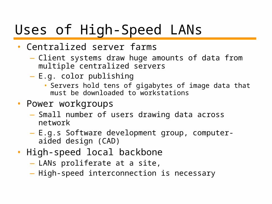
Uses of High-Speed LANs• Centralized server farms

—Client systems draw huge amounts of data from multiple centralized servers

—E.g. color publishing• Servers hold tens of gigabytes of image data that must be

downloaded to workstations

• Power workgroups—Small number of users drawing data across network—E.g.s Software development group, computer-aided

design (CAD)

• High-speed local backbone—LANs proliferate at a site,—High-speed interconnection is necessary

Corporate Wide Area Networking Needs• Up to 1990s, centralized data processing model

— Dispersed employees into multiple smaller offices— Growing use of telecommuting

• Application structure changed— Client/server and intranet computing

• More reliance on PCs, workstations, and servers• GUIs gives user graphic applications, multimedia etc.• Internet access• A few mouse clicks can trigger huge volumes of data• Traffic patterns unpredictable• Average load has risen• More data transported off premises• Traditionally 80% traffic local 20% wide area• No longer applies• Greater burden on LAN backbones and on WAN

Digital Electronics Examples• Digital Versatile Disk (DVD)

—Huge storage capacity and vivid quality

• Digital camcorder—Easy for individuals and companies to make

digital video files and place on Web sites

•  Digital Still Camera—Individual personal pictures—Companies online product catalogs with full-

color pictures of every product

QoS on The Internet• IP designed to provide best-effort, fair delivery service

—All packets treated equally—As traffic grows, congestion occurs, all packet delivery slowed—Packets dropped at random to ease congestion

• Only networking scheme designed to support both traditional TCP and UDP and real-time traffic is ATM—Means constructing second infrastructure for real-time traffic

or replacing existing IP-based configuration with ATM

• Two types of traffic—Elastic traffic can adjust, over wide ranges, to changes in delay

and throughput• Supported on TCP/IP• Handle congestion by reducing rate data presented to network

Elastic Traffic• File transfer, electronic mail, remote logon, network

management, Web access• E-mail insensitive to changes in delay• User expects file transfer delay proportional to file

size and so is sensitive to changes in throughput• With network management, delay is not concern

—If failures cause congestion, network management messages must get through minimum delay

• Interactive applications, (remote logon, Web access) quite sensitive to delay 

• Even for elastic traffic QoS-based service could help

Inelastic Traffic• Inelastic traffic does not easily adapt, if at all, to

changes in delay and throughput• E.g. real-time traffic

—Voice and video

• Requirements —Throughput: minimum value may be required—Delay: e.g. stock trading—Delay variation: Larger variation needs larger buffers—Packet loss: Applications vary in packet loss that they can

sustain

• Difficult to meet with variable queuing delays and congestion losses

• Need preferential treatment to some applications• Applications need to be able to state requirements

Supporting Both• When supporting inelastic traffic, elastic

traffic must still be supported—Inelastic applications do not back off in the

face of congestion—TCP-based applications do

• When congested, inelastic traffic continues high load,—Elastic traffic crowded off—Reservation protocol can help

• Deny requests that would leave too few resources available to handle current elastic traffic

Figure 5.1 Application Delay Sensitivity and Criticality

Performance Requirements Response Time• Time it takes a system to react to a given input

—Time between last keystroke and beginning of display of result

—Time it takes for system to respond to request

• Quicker response imposes greater cost—Computer processing power—Competing requirements—Providing rapid response to some processes may penalize

others

• User response time—Between user receiving complete reply and enters next

command (think time)

• System response time—Between user entering command and complete response 

Figure 5.2 Response Time Results for High-Function Graphics

Figure 5.3 Response Time Requirements

Throughput• Higher transmission speed makes possible

increased support for different services—e.g., Integrated Services Digital Network

[ISDN] and broadband-based multimedia services

• Need to know demands each service puts on storage and communications of systems

• Services grouped into data, audio, image, and video

Figure 5.4 Required Data Rates for Various Information Types

Figure 5.5Effective Throughput

Performance Metrics• Throughput, or capacity

— Data rate in bits per second (bps)— Affected by multiplexing— Effective capacity reduced by protocol overhead

• Header bits: TCP and IPv4 at least 40 bytes• Control overhead: e.g. acknowledgements 

• Delay— Average time for block of data to go from system to system— Round-trip delay

• Getting data from one system to another plus delay acknowledgement  — Transmission delay: Time for transmitter to send all bits of packet— Propagation delay: Time for one bit to transit from source to

destination— Processing delay: Time required to process packet at source prior

to sending, at any intermediate router or switch, and at destination prior to delivering to application

— Queuing delay: Time spend waiting in queues

Example Effect of Different Types of Delay – 64kbps• Ignore any processing or queuing delays• 1-megabit file across USA (4800km)• Fiber optic link

—Propagation rate speed of light (approximately 3 108 m/s)

• Propagation delay (4800103)/(3108) = 0.016 s• In that time host transmits (64 103)(0.016) = 1024 bits

• Transmission delay (106)/(64 103) = 15.625 s• Time to transmit file is Transmission delay plus

propagation delay = 15.641 s• Transmission delay dominates propagation delay• Higher-speed channel would reduce time required

Example Effect of Different Types of Delay – 1 Gbps• Propagation delay is still the same

—Note this as it is often forgotten!

• Transmission delay (106)/(106 103) = 0.001 s• Total time to transmit file 0.017 s• Propagation delay dominates• Increasing data rate will not noticeably speed up

delivery of file• Preceding example depends on data rate,

distance, propagation velocity, and size of packet• These parameters combined into single critical

system parameter, commonly denoted a

• where• R = data rate, or capacity, of the link• L = number of bits in a packet• d = distance between source and

destination• v = velocity of propagation of the signal• D = propagation delay

a (1)

apropagation delay

transmission delayd v

L /RRDL

• Looking at the final fraction, can also be expressed:

  • For fixed packet length, a dependent on R D

product• 64-kbps link, a = 1.024 10–3• 1-Gbps link, a = 16

a (2)

alength of the transmission channel in bits

length of the packet in bits

Impact of a• Send sequence of packets and wait for acknowledgment to each

packet before sending next— Stop-and-wait protocol

• Transmission time normalized to 1: propagation time is a• a > 1• Link's bit length greater than that of packet• Assume ACK packet is small enough to ignore its transmission time• t = 0, Station A begins transmitting packet• t = 1, A completes transmission• t = a, leading edge of packet reaches B• t = 1 + a, B has received entire packet

— Immediately transmits small acknowledgment packet• T = 1 + 2a, acknowledgment arrives at A • Total elapsed time is 1 + 2a• Hence normalized rate packets can be transmitted is 1/(1 + 2a)• Same result with a < 1

Figure 5.6 Effect of a on Link Utilization

Throughput as Function of a• For a > 1 stop-and-wait inefficient

—Gigabit WANs even for large packets (e.g., 1 Mb), channel is seriously underutilized

Figure 5.7 Normalized Throughput as a Function of a for Stop-and-Wait

Improving Performance• If lots of users each use small portion of capacity,

then for each user, effective capacity is considerably smaller, reducing a—Each user has smaller data rate

• May be inadequate

• If application uses channel with high a, performance can be improved by allowing application to treat channel as pipeline—Continuous flow of packets—Not waiting for acknowledgment to individual packet

• Problems:—Flow control—Error control—Congestion control

Flow control• B may need to temporarily restrict flow of

packets —Buffer is filling up or application is temporarily

busy—By the time signal from B arrives at A, many

additional packets in the pipeline—If B cannot absorb these packets, they must

be discarded

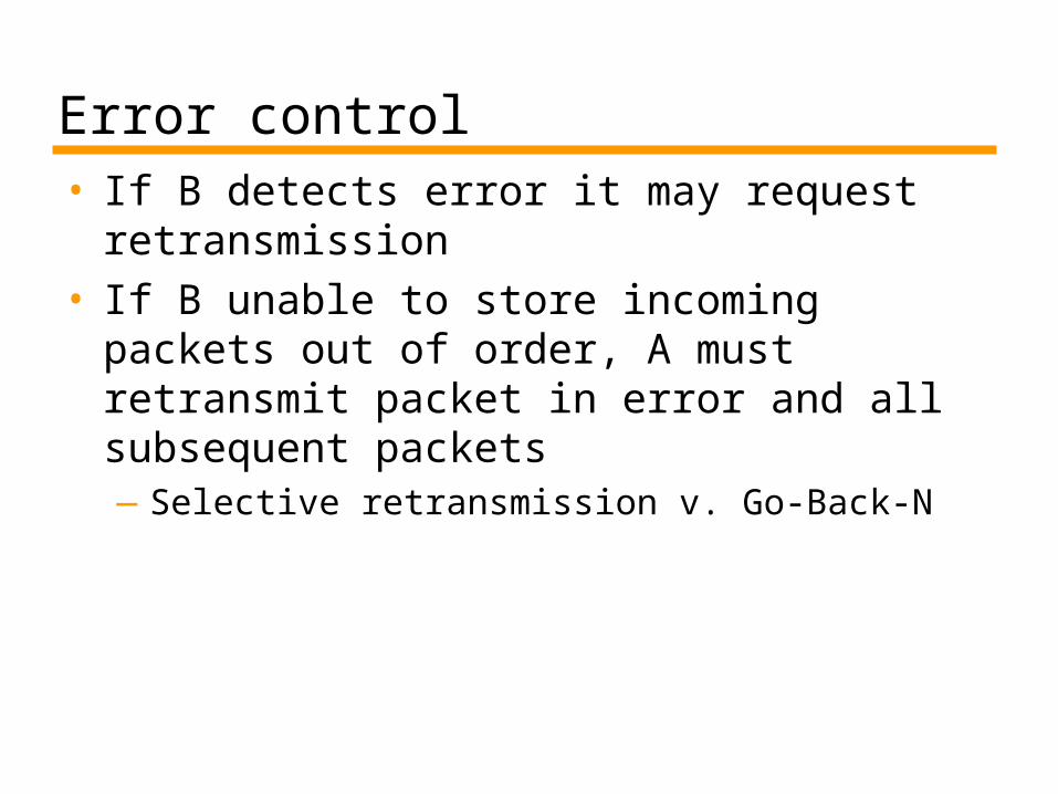
Error control• If B detects error it may request

retransmission • If B unable to store incoming packets out

of order, A must retransmit packet in error and all subsequent packets—Selective retransmission v. Go-Back-N

Congestion control• Various methods by which A can learn

there is congestion—A should reduce the flow of packets

• Large value of a—Many packets in pipeline between onset of

congestion and when A learns about it

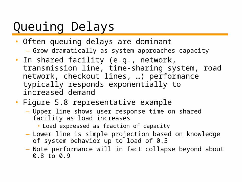
Queuing Delays• Often queuing delays are dominant

—Grow dramatically as system approaches capacity

• In shared facility (e.g., network, transmission line, time-sharing system, road network, checkout lines, …) performance typically responds exponentially to increased demand

• Figure 5.8 representative example—Upper line shows user response time on shared facility

as load increases• Load expressed as fraction of capacity

—Lower line is simple projection based on knowledge of system behavior up to load of 0.5

—Note performance will in fact collapse beyond about 0.8 to 0.9

Figure 5.8 Projected Versus Actual Response Time

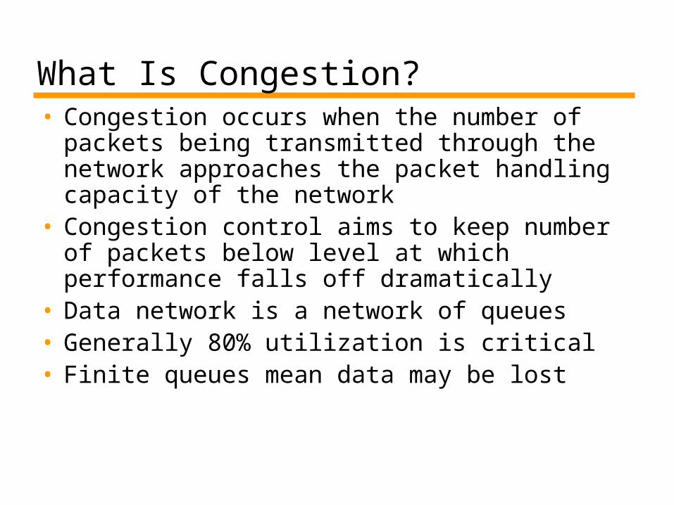
What Is Congestion?• Congestion occurs when the number of

packets being transmitted through the network approaches the packet handling capacity of the network

• Congestion control aims to keep number of packets below level at which performance falls off dramatically

• Data network is a network of queues• Generally 80% utilization is critical• Finite queues mean data may be lost

Figure 5.9 Input and Output Queues at Node

Effects of Congestion• Packets arriving are stored at input buffers• Routing decision made• Packet moves to output buffer• Packets queued for output transmitted as fast as

possible—Statistical time division multiplexing

• If packets arrive to fast to be routed, or to be output, buffers will fill

• Can discard packets• Can use flow control

—Can propagate congestion through network

Figure 5.10 Interaction of Queues in a Data Network

Figure 5.11Ideal NetworkUtilization

Practical Performance• Ideal assumes infinite buffers and no

overhead• Buffers are finite• Overheads occur in exchanging

congestion control messages

Figure 5.12The Effects of Congestion

Figure 5.13 Mechanisms for Congestion Control

Backpressure• If node becomes congested it can slow down or

halt flow of packets from other nodes• May mean that other nodes have to apply control

on incoming packet rates• Propagates back to source• Can restrict to logical connections generating

most traffic• Used in connection oriented that allow hop by

hop congestion control (e.g. X.25)• Not used in ATM nor frame relay• Only recently developed for IP

Choke Packet• Control packet

—Generated at congested node—Sent to source node—e.g. ICMP source quench

• From router or destination• Source cuts back until no more source quench

message• Sent for every discarded packet, or anticipated

• Rather crude mechanism

Implicit Congestion Signaling• Transmission delay may increase with

congestion• Packet may be discarded• Source can detect these as implicit

indications of congestion• Useful on connectionless (datagram)

networks—e.g. IP based

• (TCP includes congestion and flow control - see chapter 17)

• Used in frame relay LAPF

Explicit Congestion Signaling• Network alerts end systems of increasing

congestion• End systems take steps to reduce offered

load• Backwards

—Congestion avoidance in opposite direction to packet required

• Forwards—Congestion avoidance in same direction as

packet required

Categories of Explicit Signaling• Binary

—A bit set in a packet indicates congestion

• Credit based—Indicates how many packets source may send—Common for end to end flow control

• Rate based—Supply explicit data rate limit—e.g. ATM

Traffic Management• Fairness• Quality of service

—May want different treatment for different connections

• Reservations—e.g. ATM—Traffic contract between user and network

Flow Control• Limits amount or rate of data sent• Reasons:

—Source may send PDUs faster than destination can process headers

—Higher-level protocol user at destination may be slow in retrieving data

—Destination may need to limit incoming flow to match outgoing flow for retransmission

Flow Control at Multiple Protocol Layers• X.25 virtual circuits (level 3) multiplexed

over data link using LAPB (X.25 level 2)• Multiple TCP connections over HDLC link• Flow control at higher level applied to

each logical connection independently• Flow control at lower level applied to total

traffic

Figure 5.14 Flow Control at Multiple Protocol Layers

Flow Control Scope• Hop Scope

—Between intermediate systems that are directly connected

• Network interface—Between end system and network

• Entry-to-exit—Between entry to network and exit from

network

• End-to-end—Between end user systems

Figure 5.15Flow Control Scope

Error Control• Used to recover lost or damaged PDUs• Involves error detection and PDU

retransmission• Implemented together with flow control in

a single mechanism• Performed at various protocol levels

Self-Similar Traffic• Predicted results from queuing analysis often differ

substantially from observed performance• Validity of queuing analysis depends on Poisson nature of traffic• For some environments, traffic pattern is self-similar rather

than Poisson• Network traffic is burstier and exhibits greater variance than

previously suspected• Ethernet traffic has self-similar, or fractal, characteristic

— Similar statistical properties at range of time scales: milliseconds, seconds, minutes, hours, even days and weeks

— Cannot expect that the traffic will "smooth out" over an extended period of time

— Data clusters and clusters cluster• Merging of traffic streams (statistical multiplexer or ATM switch)

does not result in smoothing of traffic— Multiplexed bursty data streams tend to produce bursty aggregate

stream

Effects of Self-Similar Traffic (1)• Buffers needed at switches and multiplexers must be bigger

than predicted by traditional queuing analysis and simulations

• Larger buffers create greater delays in individual streams that originally anticipated

• Self-similarity appears in ATM traffic, compressed digital video streams, SS7 control traffic on ISDN-based networks, Web traffic, etc.

• Aside: self-similarity common: natural landscapes, distribution of earthquakes, ocean waves, turbulent flow, stock market fluctuations, pattern of errors and data traffic

• Buffer design and management requires rethinking— Was assumed linear increases in buffer sizes gave nearly

exponential decreases in packet loss and proportional increase in effective use of capacity

— With self-similar traffic decrease in loss less than expected, and modest increase in utilization needs significant increase in buffer size

Effects of Self-Similar Traffic (2)• Slight increase in active connections through switch can result in large

increase in packet loss• Parameters of network design more sensitive to actual traffic pattern than

expected• Designs need to be more conservative• Priority scheduling schemes need to be reexamined

— Prolonged burst of traffic from highest priority could starve other classes• Static congestion control strategy must assume waves of multiple peak

periods will occur• Dynamic strategy difficult to implement

— Based on measurement of recent traffic— Can fail to adapt to rapidly changing conditions

• Congestion prevention by appropriate sizing difficult— Traffic does not exhibit predictable level of busy period traffic

• Congestion avoidance by monitoring traffic and adapting flow control and routing difficult— Congestion can occur unexpectedly and with dramatic intensity

• Congestion recovery is complicated by need to make sure critical network control messages not lost in repeated waves of traffic

Why Have We Only Just Found Out?• Requires processing of massive

amount of data• Over long observation period• Practical effects obvious• ATM switch vendors, among others,

have found that their products did not perform as advertised—Inadequate buffering and failure to take

into account delays caused by burstiness

Required Reading• Stallings chapter 05