MNRAS 000, 1–15 (2017) Preprint 18 August 2017 Compiled using MNRAS LATEX style file v3.0

A theoretical model of the variation of the meridionalcirculation with the solar cycle

Gopal Hazra,1,2? Arnab Rai Choudhuri11Department of Physics, Indian Institute of Science, Bangalore 560012, India2Indian Institute of Astrophysics, Koramangala,Bangalore 560034, India

18 August 2017

ABSTRACTObservations of the meridional circulation of the Sun, which plays a key role in theoperation of the solar dynamo, indicate that its speed varies with the solar cycle, be-coming faster during the solar minima and slower during the solar maxima. To explainthis variation of the meridional circulation with the solar cycle, we construct a theo-retical model by coupling the equation of the meridional circulation (the φ componentof the vorticity equation within the solar convection zone) with the equations of theflux transport dynamo model. We consider the back reaction due to the Lorentz forceof the dynamo-generated magnetic fields and study the perturbations produced in themeridional circulation due to it. This enables us to model the variations of the merid-ional circulation without developing a full theory of the meridional circulation itself.We obtain results which reproduce the observational data of solar cycle variations ofthe meridional circulation reasonably well. We get the best results on assuming theturbulent viscosity acting on the velocity field to be comparable to the magnetic dif-fusivity (i.e. on assuming the magnetic Prandtl number to be close to unity). We haveto assume an appropriate bottom boundary condition to ensure that the Lorentz forcecannot drive a flow in the subadiabatic layers below the bottom of the tachocline. Ourresults are sensitive to this bottom boundary condition. We also suggest a hypothesishow the observed inward flow towards the active regions may be produced.

Key words: Sun: interior – magnetic fields

1 INTRODUCTION

The meridional circulation is one of the most importantlarge-scale coherent flow patterns within the solar convec-tion zone, the other such important flow pattern being thedifferential rotation. A strong evidence for the meridionalcirculation came when low-resolution magnetograms notedthat the ‘diffuse’ magnetic field (as it appeared in low res-olution) on the solar surface outside active regions formedunipolar bands which shifted poleward, implying a polewardflow at the solar surface (Howard & Labonte 1981; Wanget al. 1989). A further confirmation for such a flow camefrom the observed poleward migration of filaments formedover magnetic neutral lines (Makarov et al. 1983; Makarov& Sivaraman 1989). Efforts for direct measurement of themeridional circulation also began in the 1980s (Labonte &Howard 1982; Ulrich et al. 1988). The maximum velocity ofthe meridional circulation at mid-latitudes is of the order of20 m s−1.

? E-mail: hgopal@iisc.ac.in

After the development of helioseismology, there wereattempts to determine the nature of the meridional circula-tion below the solar surface (Giles et al. 1997; Braun & Fan1998). The determination of the meridional circulation in thelower half of the convection zone is a particularly challeng-ing problem. Since the meridional circulation is producedby the turbulent stresses in the convection zone, most of theflux transport dynamo models in which the meridional cir-culation plays a crucial role assume the return flow of themeridional circulation to be at the bottom of the convec-tion zone. In the last few years, several authors presentedevidence for a shallower return flow (Hathaway 2012; Zhaoet al. 2013; Schad et al. 2013). However, Rajaguru & Antia(2015) argue that helioseismic data still cannot rule out thepossibility of the return flow being confined near the bottomof the convection zone.

Helioseismic measurements indicate a variation of themeridional circulation with the solar cycle. (Chou & Dai2001; Beck et al. 2002; Basu & Antia 2010; Komm et al.2015). These results are consistent with the surface mea-surements of Hathaway & Rightmire (2010), who find that

© 2017 The Authors

arX

iv:1

708.

0520

4v1

[as

tro-

ph.S

R]

17

Aug

201

7

2 Hazra & Choudhuri

the meridional circulation at the surface becomes weakerduring the sunspot maximum by an amount of order 5 ms−1. One plausible explanation for this is the back-reactionof the dynamo-generated magnetic field on the meridionalcirculation due to the Lorentz force. The aim of this paperis to develop such a model of the variation of the meridionalcirculation and to show that the results of such a theoreticalmodel are in broad agreement with observational data.

The theory of the meridional circulation is somewhatcomplicated. The turbulent viscosity in the solar convectionzone is expected to be anisotropic, since gravity and rota-tion introduce two preferred directions at any point withinthe convection zone. A classic paper by Kippenhahn (1963)showed that an anisotropic viscosity gives rise to meridionalcirculation along with differential rotation. This work ne-glected the ‘thermal wind’ that would arise if the surfaces ofconstant density and constant pressure do not coincide. Amore complete model based on a mean field theory of con-vective turbulence is due to Kitchatinov & Ruediger (1995)and extended further by Kitchatinov & Olemskoy (2011).These authors argue that, in the high Taylor number sit-uation appropriate for the Sun, the meridional circulationshould arise from the small imbalance between the thermalwind and the centrifugal force due to the variation of theangular velocity with z (the direction parallel to the ro-tation axis). See the reviews by Kitchatinov (Kitchatinov2011, 2013) for further discussion. If the meridional circu-lation really comes from a delicate imbalance between twolarge terms, one would theoretically expect large fluctua-tions in the meridional circulation. Numerical simulationsof convection in a shell presenting the solar convection zoneproduce meridional circulation which is usually highly vari-able in space and time (Karak et al. 2014c; Featherstone &Miesch 2015; Passos et al. 2017). It is still not understoodwhy the observed meridional circulation is much more co-herent and stable than what such theoretical considerationswould suggest. There are also efforts to understand whethermean field models can produce a meridional circulation morecomplicated than a single-cell pattern (Bekki & Yokoyama2017).

The meridional circulation plays a very critical role inthe flux transport dynamo model, which has emerged asa popular theoretical model of the solar cycle. This modelstarted being developed from the 1990s (Wang et al. 1991;Choudhuri et al. 1995; Durney 1995; Dikpati & Charbon-neau 1999; Nandy & Choudhuri 2002; Chatterjee et al. 2004)and its current status has been reviewed by several au-thors (Choudhuri 2011b, 2014; Charbonneau 2014; Karaket al. 2014a). The poloidal field in this model is generatednear the solar surface from tilted bipolar sunspot pairs bythe Babcock–Leighton mechanism and then advected by themeridional circulation to higher latitudes (Dikpati & Choud-huri 1994, 1995; Choudhuri & Dikpati 1999). This polewardadvection of the poloidal field is an important feature of theflux transport dynamo model and helps in matching variousaspects of the observational data. The poloidal field even-tually has to be brought to the bottom of the convectionzone, where the differential rotation of the Sun acts on itto produce the toroidal field. If the turbulent diffusivity ofthe convection zone is assumed low, then the meridional cir-culation is responsible for transporting the poloidal field tothe bottom of the convection zone. On the other hand, if

the diffusivity is high, then diffusivity can play the domi-nant role in the transportation of the poloidal field acrossthe convection zone (Jiang et al. 2007; Yeates et al. 2008).We shall discuss this point in more detail later in the paper.Most of the authors working on the flux transport dynamoassumed a one-cell meridional circulation with an equator-ward flow at the bottom of the convection zone. This equa-torward meridional circulation plays a crucial role in theequatorward transport of the toroidal field generated at thebottom of the convection zone, leading to solar-like butter-fly diagrams. In the absence of the meridional circulation,one finds a poleward dynamo wave (Choudhuri et al. 1995).When several authors claimed to find evidence for a shal-lower meridional circulation, there was a concern about thevalidity of the flux transport dynamo model. Hazra et al.(2014) showed that, even if the meridional circulation hasa much more complicated multi-cell structure, still we canretain most of the attractive features of the flux transportdynamo as long as there is a layer of equatorward flow atthe bottom of the convection zone. In the present work, weassume a one-cell meridional circulation.

Most of the papers on the flux transport dynamo areof kinematic nature, in which the only back-reaction of themagnetic field which is often included is the so-called “α-quenching”, i.e. the quenching of the generation mechanismof the poloidal field. Usually kinematic models do not includethe back-reaction of the magnetic field on the large-scaleflows. We certainly expect the Lorentz force of the dynamo-generated magnetic field to react back on the large-scaleflows. From observations, we are aware of two kinds of back-reactions on the large-scale flows: solar cycle variations of thedifferential rotation known as torsional oscillations and so-lar cycle variations of the meridional circulation (Choudhuri2011a). There have been several calculations showing howtorsional oscillations are produced by the back-reaction ofthe dynamo-generated magnetic field (Durney 2000; Covaset al. 2000; Bushby 2006; Chakraborty et al. 2009). Rempel(2006) presented a full mean-field model of both the dynamoand the large-scale flows. This model produced both tor-sional oscillations and the solar cycle variation of the merid-ional circulation. However, apart from Figure 4(b) in thepaper showing the time-latitude plot of vθ near the bottomof the convection zone, this paper does not study the timevariation of the meridional circulation in detail. To the bestof our knowledge, this is the only mean-field calculation ofmagnetic back-reaction on the meridional circulation beforeour work.

The back-reaction on the meridional circulation shouldmainly come from the tension of the dynamo-generatedtoroidal magnetic field. Suppose we consider a ring oftoroidal field at the bottom of the convection zone. Becauseof the tension, the ring will try to shrink in size and this canbe achieved most easily by a poleward slip (van Ballegooi-jen & Choudhuri 1988). It is this tendency of poleward slipthat would give rise to the Lorentz force opposing the equa-torward meridional circulation. We show in our calculationsbased on a mean field model that this gives rise to a vortic-ity opposing the normal vorticity associated with the merid-ional circulation and, as this vorticity diffuses through theconvection zone, there is a reduction in the strength of themeridional circulation everywhere including the surface. Inorder to circumvent the difficulties in our understanding of

MNRAS 000, 1–15 (2017)

Solar cycle variation of meridional circulation 3

the meridional circulation itself, we develop a theory of howthe Lorentz force produces a modification of the meridionalcirculation with the solar cycle. The important differenceof our formalism from the formalism of Rempel (2006) isthe following. In Rempel’s formalism, one requires a properformulation of turbulent stresses to calculate the full merid-ional circulation in which one sees a cycle variation due tothe dynamo-generated Lorentz force. On the other hand, inour formalism, we have developed a theory of the modifica-tions of the meridional circulation due to the Lorentz forceso that we can study the modifications of the meridional cir-culation without developing a full theory of the meridionalcirculation.

The mathematical formulation of the theory is de-scribed in the next Section. Then Section 3 presents theresults of our simulation. Our conclusions are summarizedin Section 4.

2 MATHEMATICAL FORMULATION

Our main aim is to study how the Lorentz force due tothe dynamo-generated magnetic field acts on the meridionalcirculation. We need to solve the dynamo equations alongwith the equation for the meridional circulation.

We write the magnetic field in the form

B = Bφ(r, θ, t)eφ + ∇ × [A(r, θ, t)eφ] (1)

where Bφ is the toroidal component of magnetic field andA is the magnetic vector potential corresponding to thepoloidal component of the field. Then the dynamo equationsfor the toroidal and the poloidal components are

∂A∂t+

1s(vm.∇)(sA) = ηp

(∇2 − 1

s2

)A + S(r, θ, t), (2)

∂Bφ∂t+

1r

[∂

∂r(rvr Bφ) +

∂

∂θ(vθBφ)

]= ηt

(∇2 − 1

s2

)Bφ

+s(Bp .∇)Ω +1r

dηtdr

∂(rBφ)∂r

, (3)

where vr and vθ are components of the meridional flow vm,Ω is the differential rotation and s = r sin θ, whereas S(r, θ, t)is the source function which incorporates the Babcock-Leighton mechanism and magnetic buoyancy as explainedin Chatterjee et al. (2004) and Choudhuri & Hazra (2016).We have kept most of the parameters the same as in Chat-terjee et al. (2004). In the kinematic approach, both vm =vrer + vθeθ and Ω are assumed to be given.

To understand the effect of the Lorentz force on themeridional circulation, we need to consider the Navier-Stokes equation with the Lorentz force term, which is

∂v∂t+ (v.∇)v = − 1

ρ∇p + g + FL + Fν(v) (4)

where v is the total plasma velocity, g is the force due togravity, FL is the Lorentz force term and Fν(v) is the tur-bulent viscosity term corresponding to the velocity field v.We would have Fν(v) = ν∇2v if the turbulent viscosity ν isassumed constant in space, but Fν(v) can be more compli-cated for spatially varying ν. For simplicity we have consid-ered turbulent viscosity as a scalar quantity but, in reality,

it is a tensor and can be a quite complicated quantity: seeKitchatinov & Olemskoy (2011). It may be noted that thetensorial nature of turbulent viscosity is quite crucial in thetheory of the unperturbed meridional circulation and it can-not be treated as a scalar in the complete theory. To studytorsional oscillations, we have to consider the φ componentof Eq. 4 as done by Chakraborty et al. (2009). To considervariations of the meridional circulation, however, we need tofocus our attention on the r and θ components of Eq. 4. Aparticularly convenient approach is to take the curl of Eq. 4(noting that (v.∇)v = −v× (∇ × v)+ 1

2∇(v2)) and consider the

φ component of the resulting equation. This gives

∂ωφ

∂t− [∇ × v × (∇ × v)]φ =

1ρ2 [∇ρ × ∇p]φ (5)

+ [∇ × FL]φ + [∇ × Fν(vm)]φ .

where ω = ∇ × v is the vorticity, of which the φ componentcomes from the meridional circulation vm only. Writing v =vm + r sin θΩeφ, a few steps of straightforward algebra give

[∇ × v × (∇ × v)]φ = −r sin θ∇.(vm

ωφ

r sin θ

)+ r sin θ

∂Ω2

∂z(6)

Substituting this in Eq. 5, we have

∂ωφ

∂t+ s∇.

(vm

ωφ

s

)= s

∂Ω2

∂z+

1ρ2 (∇ρ × ∇p)φ (7)

+ [∇ × FL]φ + [∇ × Fν(vm)]φ .

We now break up the meridional velocity into two parts:

vm = v0 + v1, (8)

where v0 is the regular meridional circulation the Sun wouldhave in the absence of magnetic fields and v1 is its modifi-cation due to the Lorentz force of the dynamo-generatedmagnetic field. The azimuthal vorticity ωφ can also be bro-ken into two parts corresponding to these two parts of themeridional circulation:

ωφ = ω0 + ω1. (9)

It is clear from Eq. 7 that the regular meridional circula-tion of the Sun in the absence of magnetic fields, which isassumed independent of time in a mean field model, shouldbe given by

s∇.(v0ω0s

)= s

∂Ω2

∂z+

1ρ2 (∇ρ × ∇p)φ (10)

+ [∇ × Fν(v0)]φ .

This is the basic equation which has to be solved to developa theory of the regular meridional circulation. The first termin R.H.S is the centrifugal force term, whereas the secondterm, which can be written as

1ρ2 (∇ρ × ∇p)φ = −

g

cpr∂S∂θ, (11)

is the thermal wind term. This is the term which couplesthe theory to the thermodynamics of the Sun. So we need tosolve the energy transport equation of the Sun in order to de-velop a theory of the regular meridional circulation, makingthe problem particularly difficult. In the pioneering study ofKippenhahn (1963), the thermal wind term was neglected.

MNRAS 000, 1–15 (2017)

4 Hazra & Choudhuri

However, we now realize that for the Sun, in which the Tay-lor number is large, this term has to be important and ofthe order of the centrifugal term (Kitchatinov & Ruediger1995). It may be mentioned that, in the model of the merid-ional circulation due to Kitchatinov & Ruediger (1995) andKitchatinov & Olemskoy (2011), the advection term on theL.H.S. of Eq. 10 was neglected. On inclusion of this term,the results were found not to change much (L. Kitchatinov,private communication).

We now subtract Equation 10 from 7, which gives

∂ω1∂t+ s∇.

(v0ω1s

)+ s∇.

(v1ω0s

)(12)

= [∇ × FL]φ + [∇ × Fν(v1)]φ

on neglecting the quadratic term in perturbed quantitiesv1ω1 and assuming that Fν(v) is linear in v, which is thecase if we use the standard expressions of the viscous stresstensor. We have also assumed that the dynamo-generatedmagnetic fields do not affect the thermodynamics signifi-cantly, making the thermal wind term to drop out of Eq. 12.This is what makes the theory of the modification of themeridional circulation decoupled from the thermodynamicsof the Sun and simpler to handle than the theory of the un-perturbed meridional circulation. We have also not includedthe centrifugal force term, on the assumption that the tem-poral variations in Ω with the solar cycle do not significantlyaffect our model of the meridional circulation perturbations.The existence of torsional oscillations indicates that this maynot be a fully justifiable assumption. In a future work, weplan to include torsional oscillations in the theory along withthe meridional circulation perturbations.

In order to study how the meridional circulation evolveswith the solar cycle due to the Lorentz force of the dynamo-generated magnetic fields, we need to solve Equation 12along with Equations 2 and 3. A solution of Eq. 12 firstyields the perturbed vorticity ω1 at different steps. We canthen compute the perturbed velocity v1 in the following way.Since ∇ · ρv1 = 0, we can write v1 in terms of a stream func-tion:

v1 =1ρ∇ × [ψ(r, θ, t)eφ]. (13)

Putting this in ω1 = ∇ × v1, we get

1ρ[∇ρ × ∇ × (ψeφ)]φ +

(∇2 − 1

s2

)ψ = −ρω1. (14)

This is similar to Poisson’s equation and we solve it for agiven vorticity to get the stream function. After obtainingthe stream function, it is very trivial to get the velocityfields. There are various methods to solve this vorticity-stream function equation (Eq. 14), but we choose to solve itusing Alternating Direction Implicit (ADI) method. The ad-vantage of this method is that it will take less iterations thanthe other relaxation methods (e.g, Jacobi iteration method)to achieve the same accuracy level. To check whether thismethod is giving us the correct results, we take the vortic-ity of the unperturbed meridional circulation that we use inour dynamo calculations. We invert this vorticity to obtainthe velocity field by solving Eq. 14 and then cross check ifwe have succeeded in reproducing the original input merid-ional circulation. The stream function corresponding to theinput velocity field is shown in Figure 1(a). Here black solid

contours surrounding regions of positive stream function (in-dicated by red) imply clockwise flow and black dashed con-tours surrounding regions of negative stream function (indi-cated by blue) imply anti-clockwise flow. We calculate thevorticity (Fig 1(b)) from this given velocity field and solveEq. 14 to get back the stream function. The stream func-tion obtained in this process is shown in Fig 1(c). As we cansee, it is almost indistinguishable from the original givenstream function. While solving Eq. 14, we have set the tol-erance level to 10−5, which is found to be sufficient enough toget accurate results. As meridional circulation cannot pen-etrate much below the tachocline, we have used vr = 0 atr = 0.65R as our bottom boundary condition.

It may be noted that a realistic specification of densityρ is more important for studying the meridional circulationthan for the dynamo problem. It is the density stratificationwhich determines how strong the poleward flow at the sur-face will be compared to the equatorward flow at the bottomof the convection zone. We use a polytropic, hydrostatic, adi-abatic stratification for density that matches the standardsolar model quite well (Jones et al. 2011):

ρ = ρi

(ζ(r)ζ(r1)

)n(15)

where

ζ(r) = c0 + c1r2 − r1

r(16)

c0 =2ζ0 − β − 1

1 − β (17)

c1 =(1 + β)(1 − ζ0)(1 − β)2

(18)

and

ζ0 =β + 1

β exp(Nρ/n) + 1. (19)

Here ρi = ρ(r1) = 0.1788 g cm−3, β = r1/r2 = 0.55 is theaspect ratio, n = 1.5 is the polytropic index, and Nρ = 5 isthe number of density scale heights across the computationaldomain, which extends from r1 = 0.55R to r2 = R.

To solve Eq. 12, we need explicit expressions of [∇×FL]φand [∇×Fν(v1)]φ. If the magnetic field is given by Eq. 1, thenwe have

[∇ × FL]φ =[∇ ×

((∇ × B) × B

4πρ

)]φ

(20)

=

[1

4πρ∇ × (∇ × B) × B

]φ

−[(∇ × B) × B × ∇

(1

4πρ

)]φ

It is straightforward to show that

∇ × [(∇ × B) × B]φ (21)

=

[1r∂

∂r

(jφs

)∂(sA)∂θ

− 1r∂

∂θ

(jφs

)∂(sA)∂r

]+

[1r∂

∂θ

(Bφs

)∂(sBφ)∂r

− 1r∂

∂r

(Bφs

)∂(sBφ)∂θ

]where jφ = (∇×B)φ is φ component of current density, whichis associated only with the poloidal field. It is clear fromEq. 21 that the Lorentz forces due to the poloidal field anddue to the toroidal field clearly separate out. In typical flux

MNRAS 000, 1–15 (2017)

Solar cycle variation of meridional circulation 5

(a) Input Stream function

0.06

0.04

0.02

0.00

0.02

0.04

0.06

(b) Vorticity (ω0 ×108 )

60

40

20

0

20

40

60

(c) Reproduced Stream function

0.06

0.04

0.02

0.00

0.02

0.04

0.06

Figure 1. (a) The input stream function for the unperturbed meridional circulation which is used in all of our simulations. The

streamlines are indicated by contours—solid contours indicating clockwise flow and dashed contours indicating anti-clockwise flow. (b)The unperturbed vorticity calculated from the stream function shown in (a). Solid and dashed contours indicate positive and negative

vorticity. (c) The stream function by inverting the vorticity shown in (b) with the help of Eq. 14. This has to be compared with (a). Blue

dashed line represents the tachocline in all plots

transport dynamo simulations, the toroidal magnetic fieldturns out to be about two orders of magnitude stronger thanthe poloidal magnetic field. Since the Lorentz force goes asthe square of the magnetic field, the Lorentz force due tothe toroidal field should be about four orders of magnitudestronger than that due to the poloidal field. So we includethe Lorentz force due to the toroidal field alone in our calcu-lations. We also have to keep in mind that the magnetic fieldin the convection zone is highly intermittent with a fillingfactor, say f . The Lorentz force is significant only inside theflux tubes and a mean field value of this has to be includedin the equations of our mean field theory. This point was dis-cussed by Chakraborty et al. (2009), who showed that, if weuse mean field values of the magnetic field in our equations,then the mean field value of the quadratic Lorentz force willinvolve a division by f . Keeping this in mind, the expressionof [∇×FL]φ to be used when solving Equation 12 is obtainedfrom Equations 20 and 21:

[∇ × FL]φ =1

4πρ f

[1r2

∂

∂θ(B2φ) −

cot θr

∂

∂r(B2φ)]

(22)

+1

4πρ2 fdρdr

Bφr sin θ

∂(sin θBφ)∂θ

The expression for [∇ × Fν(v1)]φ happens to be rather com-plicated (even when the turbulent diffusivity ν is assumed tobe a scalar) and will be discussed in Appendix A. We carryon our calculations assuming a simpler form of the viscosityterm:

[∇ × Fν(v1)]φ = ν(∇2 − 1

r2 sin2 θ

)ω1. (23)

As we shall show in Appendix A, this simple expression of[∇ × Fν(v1)]φ, which is easy to implement in a numericalcode, captures the effect of viscosity reasonably well.

To study the variations of the meridional circulationwith the solar cycle, we need to solve Equations 2, 3 and 12simultaneously, with [∇ × FL]φ and [∇ × Fν(v1)]φ in Eq. 12

given by Eq. 22 and Eq. 23 respectively. It is the term [∇ ×FL]φ in Eq. 12 which is the source of the perturbed vorticityω1 and gives rise the variations of the meridional circulationwith the solar cycle. The toroidal field field Bφ obtained ateach time step from Eq. 3 is used for calculating [∇ × FL]φas given by Eq. 22.

The numerical procedure for solving Equations 2 and3 has been discussed in detail by Chatterjee et al. (2004).We solve Eq. 12 also in a similar way. Note that this equa-tion consists of two advection terms in the LHS and onediffusion term along with the source term in the RHS. Itis also basically an advection-diffusion equation similar toEq. 2 and 3. We solve Equation 12 to obtain the axisym-metric perturbed vorticity ω1 in the r − θ plane of the Sunwith 256 × 256 grid cells in latitudinal and radial directions.As in the case of Equations 2 and 3, we solve Eq. 12 byusing Alternating Direction Implicit (ADI) method of dif-ferencing, treating the diffusion term through the Crank–Nicholson scheme and the advection term through the Lax–Wendroff scheme (for more detail please see the guide ofSurya code which is publicly available upon request. Pleasesend e-mail to arnab@iisc.ac.in). We have used ω1 = 0 asthe boundary condition at the poles θ = 0 and π. The radialboundary conditions are also ω1 = 0 on the surface (r = R)and below the tachocline (r = 0.70R).

We now make one important point. By solving Eq. 12,we obtain the perturbed vorticity ω1 at each time step. If weneed the perturbed velocity v1 also at a time step, then wefurther need to solve Eq. 14 over our 256×256 grid points. Ifthis is done at every time step, then the calculation becomescomputationally very expensive. It is much easier to run thecode if we do not need v1 at each time step. In a completelyself-consistent theory, the meridional flow appearing in thedynamo Equations 2 and 3 should be given by Eq. 8, withv1 inserted at each time step. As we pointed out, this iscomputationally very expensive. If v1 is assumed small com-pared to v0, then the dynamo Equations 2 and 3 can be

MNRAS 000, 1–15 (2017)

6 Hazra & Choudhuri

solved much more easily by using vm = v0. Additionally, v1appears in the third term on the LHS of Eq. 12. We discussthis term in Appendix B, where we argue that our resultsshould not change qualitatively on not including this term.If we neglect this term along with using vm = v0 in the dy-namo equations 2 and 3, then we do not require v1 at eachtime step. The calculations in the present paper are doneby following this approach, which is computationally muchless intensive. This has enabled us to explore the parameterspace of the problem more easily and understand the basicphysics issues. We are now involved in the much more com-putationally intensive calculations in which v1 is calculatedat regular time intervals and the dynamo equations 2 and 3are solved by including v1 in the meridional flow. The resultsof these calculations will be presented in a future paper.

Finally, before presenting our results, we want to pointout a puzzle which we are so far unable to resolve. Ourcalculations suggest that the variations of the meridionalcirculation should be about two orders of magnitude largerthan what they actually are! Since a larger f would reducethe Lorentz force given by Eq. 22, we can make the variationsof the meridional circulation to have the right magnitudeonly if we take the filling factor f larger than unity, whichis clearly unphysical. We show that this problem becomesapparent even in a crude order-of-magnitude estimate. Weexpect ω1 to be of order V/L, where V is the perturbedvelocity amplitude and L is the length scale. Then ∂ω1/∂thas to be of order V/LT . Taking T to be the solar cycleperiod and L to be the depth of the convection zone, a valueV ≈ 5 m s−1 gives ∂ω1∂t

≈ 10−16s−2. (24)

The curl of the Lorentz force is the source of this term andshould be of the same amplitude. Now the curl of the Lorentzforce is of order |B2

φ/4π f ρL2 |. In a mean field dynamo model,

the magnetic field should be scaled such that the mean po-lar field comes out to have amplitude of order 10 G. Thenthe mean toroidal field at the bottom of the toroidal fieldturns out to be about 103 G. On using such a value, the curlof the Lorentz force is of order 10−15/ f s−2. This would be-come equal to 10−16 s−2 given in Eq. 24 only if f is of order10—a completely unphysical result. If we take f less than1 as expected, then the theoretical value of the perturbedmeridional circulation would be much larger than what is ob-served. One may wonder if the same problem would be therein the theory of torsional oscillations. It turns out that thetorsional oscillations have the same amplitude 5 m s−1 asvariations in the meridional circulation. However, torsionaloscillations are driven by the component ≈ |Br Bφ/L | of the

magnetic stress rather than the component ≈ |B2φ/L | rel-

evant for meridional circulation variations. Since |Br | turnsout to be about 100 times smaller |Bφ | in mean field dynamocalculations, things come out quite reasonably in the theoryof torsional oscillations (Chakraborty et al. 2009). Here isthen the puzzle. Since the variations in the meridional cir-culation are driven by the magnetic stress ≈ |B2

φ/L | which is

about 100 times larger than the magnetic stress ≈ |Br Bφ/L |driving torsional oscillations, one would naively expect themeridional circulation variations to have an amplitude about100 times larger than the amplitude of torsional oscillations.But why are their observational values found comparable?

0.55 0.65 0.75 0.85 0.95

R¯

108

109

1010

1011

1012

1013

η

ηp

ηt

Figure 2. Magnetic diffusivities (cm2 s−1) used in our flux trans-

port model. The black solid line shows the turbulent diffusivityfor the poloidal magnetic field, and the blue solid line shows the

same for the toroidal magnetic field.

In the present paper, we do not attempt to provide any so-lution to this puzzle and merely present this as an issuethat requires further study. We point out that, even in non-magnetic situations, some terms in the equations tend toproduce a much faster meridional circulation than what isobserved (Durney 1996; Dikpati 2014). Presumably, such afast meridional circulation would upset the thermal balanceand, as a back reaction, a thermal wind force would ariseto ensure that such a large meridional circulation does nottake place. It needs to be investigated whether similar con-siderations would hold in the case of magnetic forcing of themeridional circulation as well.

3 RESULTS

We now present results obtained by solving the dynamoequations 2 and 3 simultaneously with Eq. 12 for perturbedvorticity. The various dynamo parameters—the source func-tion S(r, θ, t), the differential rotation Ω, the meridional circu-lation vm and the turbulent diffusivities ηp, ηt—are specifiedas in Chatterjee et al. (2004). As we have pointed out, cal-culations in this paper are based on using the unperturbedmeridional circulation v0 in the dynamo equations 2 and 3.We also follow Chatterjee et al. (2004) in assuming differentdiffusivity for the poloidal and the toroidal components ofthe magnetic field as shown in Fig. 2. The justification forthe reduced diffusivity of the toroidal component is that itis much stronger than the poloidal component and the effec-tive turbulent diffusivity experienced by it is expected to bereduced by the magnetic quenching of turbulence. The un-quenched value of turbulent diffusivity used for the poloidalfield inside the convection zone is what is expected fromsimple mixing length arguments (Parker (1979), p. 629). Amuch smaller value of turbulent diffusivity was assumed insome other flux transport dynamo models (Dikpati & Char-bonneau 1999). However, a higher value appears much morerealistic on the ground that only with such a higher value

MNRAS 000, 1–15 (2017)

Solar cycle variation of meridional circulation 7

0 5 10 15 20 25 30 35Time (years)

0

1

2

3

4

5

6

vort

icity

(with

ω1

=0

at r

=0.

70R¯)

41

42

43

44

45

46

47

vort

icity

(with

ω1

=0

at r

=0.

55R¯)

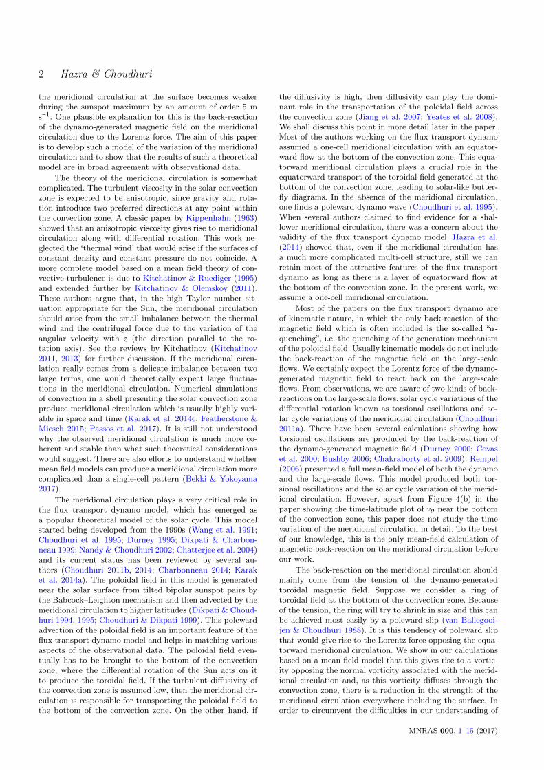
Figure 3. The perturbed vorticity at a point within the convec-

tion zone is plotted against time for the two cases with differ-ent boundary conditions. The black solid line shows the absolute

value of the perturbed vorticity ω1 at 15 latitude and at depth

0.75R, with the bottom boundary condition ω1 = 0 at r = 0.7R.The blue dashed line shows the absolute value of perturbed vor-

ticity ω1 at 15 latitude and at depth 0.71R, with the bottomboundary condition ω1 = 0 at r = 0.55R. The values of the vor-

ticity which is shown in blue dashed line are given on the right

y-axis with blue colour.

it is possible to model many different aspects of observa-tional data: such as the dipolar parity (Chatterjee et al.2004; Hotta & Yokoyama 2010), the lack of significant hemi-spheric asymmetry (Chatterjee & Choudhuri 2006; Goel &Choudhuri 2009), the correlation of the cycle strength withthe polar field during the previous minimum (Jiang et al.2007) and the Waldmeier effect (Karak & Choudhuri 2011).For solving the vorticity Equation 12 we need to specify theturbulent viscosity ν. From simple mixing length arguments,we would expect the turbulent magnetic diffusivity ηp andthe turbulent viscosity ν to be comparable, i.e, we wouldexpect the magnetic Prandtl number Pm = ν/ηp to be closeto 1. We first present results obtained with Pm = 1 in Sec-tion 3.1. How our results get modified on using a lower valueof the magnetic Prandtl number Pm will be discussed in theSection 3.2.

We know that the toroidal field Bφ changes its sign fromone cycle to the next. Since the Lorentz force depends on thesquare of Bφ, as seen in Eq. 22, the Lorentz force should havethe same sign in different cycles. As a result, one may thinkthat the perturbed vorticity ω1 driven by the Lorentz forcewill tend to grow. However, results presented in Sections 3.1and 3.2 are obtained with the boundary condition ω1 = 0at r = 0.7R, which ensures that ω1 cannot grow indefi-nitely. Asymptotically, we find ω1 to have oscillations as theLorentz force increases during solar maxima and decreasesduring solar minima. In Fig. 3 we have shown the time vari-ation of perturbed vorticity (at 15 latitude and r = 0.75R)for this case with the black solid line. The calculations pre-sented in Sec. 3.3 were done by taking the boundary condi-tion ω1 = 0 at r = 0.55R. In this situation, we found thatω1 has oscillations around a mean which keeps growing withtime (see the blue dashed line plot of Fig. 3 which does notsaturate even after running the code for several cycles).

3.1 Results with Pm = 1

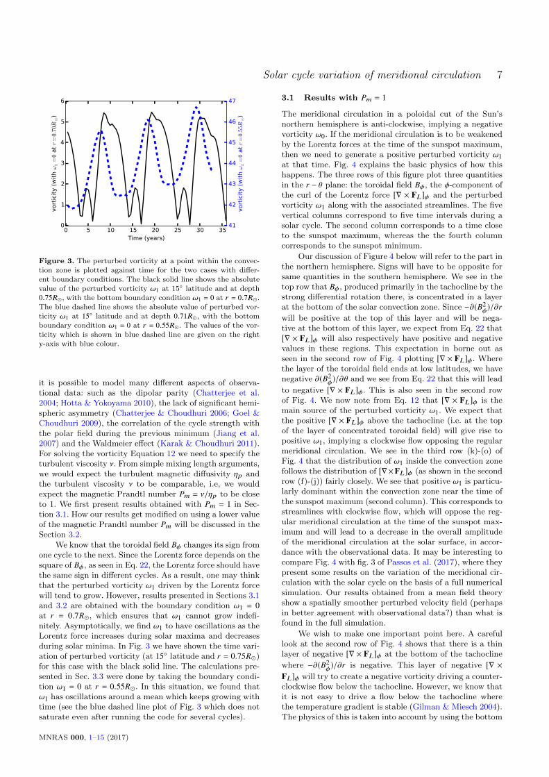
The meridional circulation in a poloidal cut of the Sun’snorthern hemisphere is anti-clockwise, implying a negativevorticity ω0. If the meridional circulation is to be weakenedby the Lorentz forces at the time of the sunspot maximum,then we need to generate a positive perturbed vorticity ω1at that time. Fig. 4 explains the basic physics of how thishappens. The three rows of this figure plot three quantitiesin the r − θ plane: the toroidal field Bφ, the φ-component ofthe curl of the Lorentz force [∇ × FL]φ and the perturbedvorticity ω1 along with the associated streamlines. The fivevertical columns correspond to five time intervals during asolar cycle. The second column corresponds to a time closeto the sunspot maximum, whereas the the fourth columncorresponds to the sunspot minimum.

Our discussion of Figure 4 below will refer to the part inthe northern hemisphere. Signs will have to be opposite forsame quantities in the southern hemisphere. We see in thetop row that Bφ, produced primarily in the tachocline by thestrong differential rotation there, is concentrated in a layerat the bottom of the solar convection zone. Since −∂(B2

φ)/∂rwill be positive at the top of this layer and will be nega-tive at the bottom of this layer, we expect from Eq. 22 that[∇ × FL]φ will also respectively have positive and negativevalues in these regions. This expectation in borne out asseen in the second row of Fig. 4 plotting [∇ × FL]φ. Wherethe layer of the toroidal field ends at low latitudes, we havenegative ∂(B2

φ)/∂θ and we see from Eq. 22 that this will lead

to negative [∇ × FL]φ. This is also seen in the second rowof Fig. 4. We now note from Eq. 12 that [∇ × FL]φ is themain source of the perturbed vorticity ω1. We expect thatthe positive [∇ × FL]φ above the tachocline (i.e. at the topof the layer of concentrated toroidal field) will give rise topositive ω1, implying a clockwise flow opposing the regularmeridional circulation. We see in the third row (k)-(o) ofFig. 4 that the distribution of ω1 inside the convection zonefollows the distribution of [∇×FL]φ (as shown in the secondrow (f)-(j)) fairly closely. We see that positive ω1 is particu-larly dominant within the convection zone near the time ofthe sunspot maximum (second column). This corresponds tostreamlines with clockwise flow, which will oppose the reg-ular meridional circulation at the time of the sunspot max-imum and will lead to a decrease in the overall amplitudeof the meridional circulation at the solar surface, in accor-dance with the observational data. It may be interesting tocompare Fig. 4 with fig. 3 of Passos et al. (2017), where theypresent some results on the variation of the meridional cir-culation with the solar cycle on the basis of a full numericalsimulation. Our results obtained from a mean field theoryshow a spatially smoother perturbed velocity field (perhapsin better agreement with observational data?) than what isfound in the full simulation.

We wish to make one important point here. A carefullook at the second row of Fig. 4 shows that there is a thinlayer of negative [∇ × FL]φ at the bottom of the tachocline

where −∂(B2φ)/∂r is negative. This layer of negative [∇ ×

FL]φ will try to create a negative vorticity driving a counter-clockwise flow below the tachocline. However, we know thatit is not easy to drive a flow below the tachocline wherethe temperature gradient is stable (Gilman & Miesch 2004).The physics of this is taken into account by using the bottom

MNRAS 000, 1–15 (2017)

8 Hazra & Choudhuri

(a) (b) (c) (d) (e)

1.2

0.9

0.6

0.3

0.0

0.3

0.6

0.9

1.2

Bφ

(f) (g) (h) (i) (j)

200

150

100

50

0

50

100

150

200

[∇×FL ]φ ×1020

(k) (l) (m) (n) (o)

8

6

4

2

0

2

4

6

8

ω1 ×108

Figure 4. Snapshots in the r − θ plane of different quantities spanning an entire solar cycle: the toroidal field Bφ , the φ component ofthe curl of the Lorentz force [∇ × FL ]φ and the perturbed vorticity ω1 with streamlines are shown in the first row (a)-(e), the secondrow (f)-(j), and the third row (k)-(o) respectively. The five columns represent time instants during the midst of the rising phase, the

solar maximum, the midst of the decay phase and the solar minimum, followed by the midst of the rising phase again. In the thirdrow (k)-(o), the solid black contours represent clockwise flows and the dashed black contours represent anti-clockwise flows. The unit of

toroidal fields in the first row is given in terms of Bc . The Lorentz forces in the second row also are calculated from toroidal fields in

the unit of Bc . The vorticities are given (third row) in s−1. Here Bc is the critical strength of magnetic fields above which the fields aremagnetically buoyant and create sunspots (Chatterjee et al. 2004). All the plots are for the magnetic Prandtl number Pm = 1 with thebottom boundary condition ω1 = 0 at r = 0.7R.

boundary condition that ω1 = 0 at r = 0.7R. As we shall seein Section 3.3, results can change dramatically on changingthis boundary condition. Our boundary condition ensuresthat the negative [∇ × FL]φ at the bottom of the tachoclinecannot produce negative vorticity there (as seen in the thirdrow of Fig. 4) and cannot drive a flow below the tachocline.

We thus see that, while the distribution of ω1 follows thedistribution of [∇×FL]φ fairly closely within the convectionzone, this is not the case at the bottom of the tachocline.

The strength of the perturbed meridional circulationcertainly depends on the strength of [∇×FL]φ, which is con-trolled by the filling factor f as seen in Eq. 22. We have

MNRAS 000, 1–15 (2017)

Solar cycle variation of meridional circulation 9

15 20 25 30 35 40 45 50Time (years)

50

0

50

Latit

udes

(a) v1 (r=0.99R¯)

6.04.53.01.5

0.01.53.04.56.0

m/s

15 20 25 30 35 40 45 50Time (years)

50

0

50

Latit

udes

(b) v1 (r=0.75R¯)

1.00

0.75

0.50

0.25

0.00

0.25

0.50

0.75

1.00m/s

Figure 5. The time–latitude plot of perturbed velocities vθ (a) near the surface (r = 0.99R) and (b) at the depth r = 0.75R. In the

northern hemisphere, positive red colour shows perturbed flows towards the equator and the negative blue colour shows flows towardspole. It is opposite in the southern hemisphere. Toroidal fields at the bottom of the convection zone are overplotted in both of the plots

by line contours. Black solid contours indicate positive polarity and black dashed contours are for negative polarity. All the plots are forthe magnetic Prandtl number Pm = 1 with the bottom boundary condition ω1 = 0 at r = 0.7R.

13 16 19 22 25 28 31 34 37Time (years)

0

3

6

9

12

15

18

21

24

Velo

city

(m/s

)

Meridional flowSSN

Figure 6. The variation of the total meridional circulation withtime is plotted with solar cycle. The yearly averaged solar cycle

is plotted in the red solid line, whereas the black dashed lineshows the total meridional circulation just below the surface at

25 latitude.

followed the dynamo model of Chatterjee et al. (2004) inwhich the scale of the magnetic field is set by the criticalvalue Bc above which the toroidal field becomes buoyant inthe convection zone. As pointed out by Jiang et al. (2007)and followed by Chakraborty et al. (2009), we take Bc = 108G to ensure that the mean polar field has the right ampli-tude. With the unit of the magnetic field fixed in this way, wefind that f = 53 gives surface values of the perturbed merid-ional circulation of the order of 5 m s−1 comparable to whatis seen in the observational data. Such a value of the fillingfactor f , which should be less than 1, is completely unphys-ical. We anticipated this problem on the basis of the order-

of-magnitude estimate presented in Section 2. Chakrabortyet al. (2009) needed f = 0.067 to model torsional oscillations,whereas Choudhuri (2003) estimated that it should be aboutf ≈ 0.02. Since f appears in the denominator of the Lorentzforce term in Eq. 22, a large value of f means that we haveto reduce the Lorentz force in an artificial manner to matchtheory with observations. We are not sure about the signif-icance of this. All we can say now is that, if we reduce theLorentz force in this manner, then we find theoretical resultsto be in good agreement with observational data.

Fig. 5 shows time-latitude plots of the perturbed vθ justbelow the surface and in the lower part of the convectionzone. Fig. 5(a) can be directly compared with Fig. 11 ofKomm et al. (2015). When the perturbed meridional circu-lation near the surface has an amplitude of about 5 m s−1

near the surface (comparable to what we find in observa-tional data), its amplitude at the bottom of the convectionzone turns out to be about 0.75 m s−1. This is a significantfraction of the amplitude of the meridional circulation at thebottom of the convection zone, which is of order 2 m s−1. Inother words, the ratio of the amplitude at the bottom of theconvection zone to the amplitude at the top of the convec-tion zone for the perturbed meridional circulation (≈ 0.15)is somewhat larger than this ratio for the regular meridionalcirculation(≈ 0.08). The reason behind this becomes clear oncomparing the distribution of ω0, as seen in Fig. 1(b), withthe distribution of ω1, as seen in Fig. 4(l), i.e. the secondfigure in the third row of Fig. 4. This ratio is small whenthe vorticity is concentrated near the upper part of the con-vection zone and streamlines in the lower part of the con-vection zone are fairly spread out. On the other hand, withω1 distributed throughout the body of the convection zone,this ratio for the perturbed meridional circulation is not sosmall. The perturbed meridional circulation at the bottomof the convection zone (which is in the poleward direction)will reduce the value of the equatorward meridional circula-tion there considerably at the time of the sunspot maximum.This will presumably affect the behaviour of the dynamo, in

MNRAS 000, 1–15 (2017)

10 Hazra & Choudhuri

(a) (b) (c) (d) (e)

32

24

16

8

0

8

16

24

32

[∇×FL ]φ ×1020

(f) (g) (h) (i) (j)

20

15

10

5

0

5

10

15

20ω1 ×108

Figure 7. Results obtained with low Prandtl number plotted in the same way as Fig. 4. The top row plotting [∇ × FL ]φ is the same as

the second row of Fig. 4. The bottom row shows the vorticity ω1 with streamlines.

5 10 15 20 25 30 35Time (years)

50

0

50

Latit

udes

(a) v1 (r=0.99R¯)

8

6

4

2

0

2

4

6

8m/s

5 10 15 20 25 30 35Time (years)

50

0

50

Latit

udes

(b) v1 (r=0.75R¯)

1.6

1.2

0.8

0.4

0.0

0.4

0.8

1.2

1.6m/s

Figure 8. Same as Fig. 5 but with low Prandtl number Pm.

such ways as lengthening its period (since a slower merid-ional circulation at the bottom of the convection zone duringcertain phases of the cycle is expected to lengthen the cycle).We are certainly not fully justified in solving the dynamoequations 2–3 by using the regular meridional circulationv0. However, as we have pointed out in Section 2, in or-der to include the perturbed meridional circulation in theseequations, we need to evaluate the perturbed velocity fieldat every time step (i.e. not only the perturbed vorticity ω1),

which will require considerably more computational efforts.We are currently doing these calculations and will presentthe results in a forthcoming paper. The aim of the presentexploratory paper is to elucidate the basic physics of theproblem and not to construct a very complete model. Fig-ure 6 shows the time evolution of the total vθ at 25 degreelatitude just below the surface along with the sunspot num-ber. We see that the meridional circulation reaches its min-

MNRAS 000, 1–15 (2017)

Solar cycle variation of meridional circulation 11

imum a little after the sunspot maximum. This figure canbe compared with Fig. 4 of Hathaway & Rightmire (2010).

One important aspect of observational data is an in-ward flow towards the belt of active regions at the time ofthe sunspot maximum (Cameron & Schussler 2010; Kommet al. 2015). We now come to the question whether our modelcan provide any explanation for this. This inward flow meansthat the meridional circulation is enhanced in the low lat-itudes below the sunspot belt and reduced in the higherlatitudes. It is thought that the cooling effect of sunspotsmay drive this inward flow (Spruit 2003; Gizon & Rempel2008). Since this idea is not yet fully established through de-tailed and rigorous calculations, it is worthwhile to look foralternative explanations. We would like to draw the reader’sattention to the first figure in the bottom row of Fig. 4.In the northern hemisphere, we see positive ω1 (implyingclockwise flow) extending over latitudes higher than wheresunspots are usually seen. However, we see a region of nega-tive ω1 (implying counter-clockwise flow) at lower latitudes.It is clear that the perturbed meridional circulation is of thenature of an inward flow at the latitudes between the re-gion of positive ω1 on the high-latitude side and the regionof negative ω1 on the low-latitude side. We are thus ableto obtain an inward flow at the latitudes where sunspotsare typically seen, but unfortunately we are getting this atthe wrong time—shortly after the sunspot minimum (whenthere would be no sunspots in that region) rather than atthe sunspot maximum. A look at Fig. 5(a) also makes itclear that this inward flow occurs slightly after the sunspotminimum. We are now exploring the question whether, bychanging some parameters of the model, it is possible to getthis inward flow at the right latitudes at the right phase(around the sunspot maximum) of the solar cycle. If our in-terpretation is correct, then the inward flow has nothing todo with the actual physical presence of sunspots. While theLorentz force above the tachocline tends to produce positivevorticity, the low-latitude edge of the toroidal magnetic fieldbelt can be a source of negative vorticity. If the sunspotbelt merely happens to be a region having positive ω1 onthe high-latitude side and negative ω1 on the low-latitudeside, then it will be a region of apparent inward flow. Wesuggest this as a tentative hypothesis which requires furtherstudy. We shall argue in Appendix B that the advectionterm s∇.(v1ω0/s) not incorporated in the present study (thethird term on the LHS of Eq. 12) may be quite importantfor modelling the inward flow in active regions.

3.2 Results with low Prandtl number (Pm < 1)

In order to study how the nature of the perturbations in themeridional circulation will change on changing the turbulentviscosity ν, we now present results obtained by taking ν = ηt(shown by the blue solid line in Fig. 2) rather than ν = ηpwhich was the case for the results presented in Section 3.1.This makes the magnetic Prandtl number defined as ν/ηp(note that ηp rather than ηt represents the unquenched tur-bulent diffusivity) much smaller than unity within the bodyof the convection zone.

We now want to present our results in the meridionalplane of the Sun. Since there have been no changes in thedynamo equations 2 and 3, the toroidal field Bφ and theφ-component of the curl of the Lorentz force [∇ × FL]φ will

be the same as in the first two rows of Fig. 4 if we take thesnapshots at the same instants of time. To facilitate easycomparison with the perturbed vorticity ω1 generated, weagain plot [∇ × FL]φ in the top row of Figure 7. This isthe same as the middle row of Fig. 4. Then the bottomrow of Figure 7 shows the perturbed vorticity ω1 along withthe streamlines of the perturbed velocity. This bottom rowshould be compared to the bottom row of Fig. 4. When ν ishigher (the case of Fig. 4), the perturbed vorticity ω1 spreadsmore evenly within the convection zone. On the other hand,when ν is lower (the case of Figure 7), the perturbed vorticityω1 tends to be frozen where it is created by [∇ × FL]φ. As aresult, ω1 follows [∇ × FL]φ more closely in Figure 7 ratherthan in Fig. 4. We thus see a more complicated distributionof ω1 in Figure 7 implying a more complicated velocity field.

To make the perturbed meridional circulation near thesurface comparable to what we find in the observationaldata, we need to choose f = 5.3× 102 in this case of low Pm.This is even more unphysical than what we needed for thecase Pm = 1 ( f = 53) with all the other dynamo parameterssame. Basically, on reducing viscosity, vorticity tends to getpiled up and we need to reduce the strength of the Lorentzforce further to match observations. The perturbed velocitiesnear the surface and near the bottom of the convection zoneare shown in Fig. 8(a) and 8(b) respectively. The require-ment that the perturbed velocity at the surface compareswith observational data forces the perturbed velocity at thebottom of the convection zone as seen in Fig. 8(b) of order1.5 m s−1, which makes it almost comparable to the un-perturbed velocity (though they are in opposite directions).This shows that solving the dynamo equations 2 and 3 withthe unperturbed meridional circulation v0 is more unjusti-fied in this case than in the case of Pm = 1.

We do not know how large the perturbations to themeridional circulation at the bottom of the convection zoneactually are. If they were comparable to the unperturbedmeridional circulation, then probably we would see some ef-fects on the dynamo. Since this problem has not been stud-ied before, we do not know what those effects may be like.As, on theoretical grounds also we expect Pm to be of orderunity, we believe that the model with Pm = 1 presented inSection 3.1 is probably a more realistic depiction of what ishappening inside the Sun rather than the model with lowPm.

3.3 Dependence of the results on lower radialboundary condition

While discussing Fig. 4, we have pointed out that theLorentz force at the bottom of the tachocline would have atendency of producing a perturbed vorticity with the samesign as the unperturbed vorticity. This will tend to drive acounter-clockwise flow (in the northern hemisphere) belowthe tachocline. Since on physical grounds we do not expectsuch a flow to be driven in a region of stable temperaturegradient, we have used the boundary condition ω1 = 0 atr = 0.70R in Sections 3.1 and 3.2 to suppress this flow.We found that our results are quite sensitive to this bot-tom boundary condition. We now discuss what we get onchanging the boundary condition to ω1 = 0 at r = 0.55R.

Again the solutions of the dynamo equations 2 and 3remain the same as in Section 3.1 and 3.2. We present the

MNRAS 000, 1–15 (2017)

12 Hazra & Choudhuri

(a) (b) (c) (d) (e)

320

240

160

80

0

80

160

240

320ω1 ×108

Figure 9. On changing the bottom boundary condition to ω1 = 0 at r = 0.55R, the third row of Fig. 4 would get changed to this.

solutions of the perturbed vorticity at the same time instantsas the time instants in Figure 4. Only the third row of thisfigure will be replaced by what is shown in Figure 9. Whenwe had taken the boundary condition ω1 = 0 at r = 0.70Rearlier, ω1 was restrained from growing indefinitely. Now, onpushing the boundary well below the bottom of the convec-tion zone, we found that ω1 kept growing for many cycles forwhich we ran the code (see Fig. 3). This is the reason why thevalues of ω1 given in the colour scale in Figure 9 are ratherlarge. We would expect the growing perturbed vorticity tohave the opposite sign of the original unperturbed vorticity.But this is not the case now. The growing perturbed vorticityhas the same sign as the original unperturbed vorticity. Thismeans that the Lorentz force strengthens the original merid-ional circulation rather than opposing it! Presumably this isbecause the effect of the Lorentz force at the bottom of thetachocline (which tries to produce a perturbed vorticity ofthe same sign as the original vorticity) overwhelms the effectof the Lorentz force at the top of the tachocline which op-poses the unperturbed meridional circulation. These resultsshow that the bottom boundary condition is quite crucial.If we allow the Lorentz force to create a perturbed vortic-ity below the bottom of the tachocline, we may get totallyunphysical results.

4 CONCLUSION

The meridional circulation of the Sun plays a crucial rolein the flux transport dynamo model, the currently favouredtheoretical model for the solar cycle. Presumably an equator-ward flow at the bottom of the convection zone is responsiblefor the equatorward migration of the sunspot belts (Choud-huri et al. 1995; Hazra et al. 2014). The poleward flow atthe surface builds up the polar field of the Sun by bring-ing together the poloidal field generated by the Babcock–Leighton mechanism from the decay of active regions (Hazraet al. 2017). We now have growing evidence that similar fluxtransport dynamos operate in other solar-like stars as well(Choudhuri 2017). Our lack of understanding of the merid-ional circulation in such stars is the major stumbling blockfor building theoretical models of stellar dynamos (Karak

et al. 2014b; Choudhuri 2017). The mathematical theory ofthe meridional circulation involves a centrifugal term and athermal wind term. The centrifugal term couples the the-ory of the meridional circulation to the theory of differentialrotation and the thermal wind term couples the theory tothe thermodynamics of the star—making it a very complexsubject.

We now have evidence that the meridional circulation ofthe Sun varies with the solar cycle, becoming weaker aroundthe sunspot maximum (Chou & Dai 2001; Beck et al. 2002;Hathaway & Rightmire 2010; Komm et al. 2015). We be-lieve that this is caused by the back-reaction of the Lorentzforce of the dynamo-generated magnetic field. We show thatthe theory of the perturbations to the meridional circula-tion caused by the Lorentz force can be decoupled from thetheory of the unperturbed meridional circulation itself. Es-pecially, this theory becomes decoupled from any thermody-namic considerations if we assume that the magnetic fieldsdo not affect the thermodynamics of the Sun. This makesthe theory of the perturbations to the meridional circula-tion much simpler than the theory of the meridional circula-tion itself. Even without having a theory of the unperturbedmeridional circulation, we are able to develop a theory ofhow the meridional circulation gets affected by the Lorentzforce of the dynamo-generated magnetic fields.

The most convenient way of developing a theory of themeridional circulation is by considering the equation for theφ-component of vorticity ωφ. We solve the equation for theperturbed vorticity along with the standard axisymmetricmean field equations of the flux transport dynamo. For theunperturbed meridional circulation, ωφ is negative in thenorthern hemisphere of the Sun. If the Lorentz force canproduce some positive vorticity there, then we expect themeridional circulation to become weaker during the sunspotmaxima. Our calculations show that positive vorticity is in-deed produced near the top of the tachocline. Our theoreti-cal results are able to explain many aspects of observationaldata presented by Hathaway & Rightmire (2010) and Kommet al. (2015) We get best results when the turbulent viscosityν is taken to be comparable to the turbulent diffusivity ηp ofthe magnetic field, i.e. when the magnetic Prandtl numberPm is close to unity. Our results are sensitive to the bound-

MNRAS 000, 1–15 (2017)

Solar cycle variation of meridional circulation 13

ary condition at the bottom of the convection zone. At thebottom of the tachocline, the Lorentz force tends to producevorticity with the same sign as the unperturbed vorticity andthis has to be suppressed with a suitable boundary conditionto incorporate the important physics that it is very difficultto drive flows in the stable subadiabatic layers below thetachocline.

One intriguing observation is that of an inward flow to-wards active regions during the sunspot maxima (Cameron& Schussler 2010; Komm et al. 2015). While we have notbeen able to construct a satisfactory model of this inwardflow, we suggest a possibility how this flow may be produced.We would have such a flow if the northern hemisphere hasa positive perturbed vorticity at latitudes above the mid-latitudes and a negative perturbed vorticity at lower lat-itudes. We propose a scenario how this can happen. TheLorentz force at the top of the tachocline tends to producepositive vorticity, whereas the Lorentz force at the edge ofthe toroidal field belt at low latitudes tends to produce nega-tive vorticity. In our model, we found an inward flow towardstypical sunspot latitudes at a wrong phase of the solar cycle.It remains to be seen whether the phase can be corrected bychanging the parameters of the problem.

One puzzle we encounter is that we have to reduce thestrength of the Lorentz force artificially by about two or-ders of magnitude to make theory fit with observations. Wepoint out that a similar problem arises in the non-magnetictheory as well. While we do not have a proper explanationfor this, we make one comment. While the overall strengthof the Lorentz force varies with the solar cycle, it does notchange sign between cycles. As a result, the Lorentz forcewould always tend to drive a very strong clockwise flowin the northern hemisphere (anti-clockwise in the south),if it is not reduced sufficiently. Now, in the theory of theunperturbed meridional circulation, we know that we needsome force trying to drive such a flow—to make the sur-faces of constant angular velocity depart from cylinders andto balance the centrifugal term. Normally, the thermal windcaused by anisotropic heat transport in the Sun is believed todo this (Kitchatinov & Ruediger 1995; Kitchatinov & Olem-skoy 2011). Is it possible that the expected large Lorentzforce also plays an important in the force balance? To ad-dress this question, one has to carry on a much more com-plicated analysis than what we have attempted in this pa-per, without separating the equations of unperturbed andperturbed meridional circulation. While we do not attemptsuch an analysis, our analysis brings out many basic physicsissues rather clearly and raises intriguing questions like this.

The equation of the perturbed meridional circulationgives us the perturbed vorticity at different times. In orderto get the perturbed velocity from the perturbed vorticity,we need to solve a Poisson-type equation. If we want todo this at every time step, then running the code becomescomputationally very expensive. On the hand, if we are sat-isfied only with the perturbed vorticity at all steps and donot require the perturbed velocity, then we need much lesscomputer time. This is what we have done in this paper inwhich our aim was to carry out a parameter space studyto understand the basic physics. However, we have to pay aprice for not calculating the perturbed velocity at all timesteps. We keep solving the dynamo equations by using theunperturbed velocity of the meridional circulation. This is

certainly a questionable approximation. If we want to makethe perturbed velocity at the surface comparable to whatis found in observational data (≈ 5 m s−1), then the per-turbed velocity at the bottom of the convection zone turnsout to be ≈ 0.75 m s−1. This is certainly smaller than the un-perturbed velocity there (≈ 2 m s−1), but is not completelynegligible. While we feel reassured that the perturbed ve-locity at the bottom of the convection zone is smaller thanthe unperturbed velocity and probably will not necessitatea major revision of the flux transport dynamo, the effect ofthis perturbed velocity on the dynamo needs to be investi-gated. We are now in the process of including this perturbedvelocity in the dynamo equations. This will need finding theperturbed velocity from the perturbed vorticity at differenttime intervals—pushing up the computational requirementssignificantly. Once we do that, we shall be able to includeanother advection term involving v1 in the computationswhich had been left out in this paper because of computa-tional difficulties. This term may be important for modellingthe inward flow towards active regions.

Not including the back-reactions on the meridional cir-culation in the dynamo equations is not a limitation of thispaper alone, but a limitation of nearly all hitherto pub-lished papers on the flux transport dynamo based on 2Dkinematic mean field formulation. To the best of our knowl-edge, only Karak & Choudhuri (2012) studied this problemby modelling the back-reaction on the meridional circulationdue to the Lorentz force through a simple parameterization(though see Passos et al. (2012) who have included back-reaction in a simple low-order dynamo model). Althoughsuch a back-reaction on the meridional circulation can havedramatic effects on the dynamo if the magnetic diffusivity islow, Karak & Choudhuri (2012) found that the effect is notmuch on a high-diffusivity dynamo (like what we present inthis paper). However, it is now important to go beyond suchsimple parameterization and include the properly computedperturbed velocity in the dynamo equations and study itseffects. We hope that we shall be able to present our resultsin a forthcoming paper in the near future.

ACKNOWLEDGEMENTS

We thank an anonymous referee for valuable comments. GHwould like to acknowledge CSIR, India for financial support.ARC’s research is supported by J. C. Bose fellowship grantedby DST, India.

REFERENCES

Basu S., Antia H. M., 2010, ApJ, 717, 488

Beck J. G., Gizon L., Duvall Jr. T. L., 2002, ApJ, 575, L47

Bekki Y., Yokoyama T., 2017, ApJ, 835, 9

Braun D. C., Fan Y., 1998, ApJ, 508, L105

Bushby P. J., 2006, MNRAS, 371, 772

Cameron R. H., Schussler M., 2010, ApJ, 720, 1030

Chakraborty S., Choudhuri A. R., Chatterjee P., 2009, PhysicalReview Letters, 102, 041102

Charbonneau P., 2014, ARA&A, 52, 251

Chatterjee P., Choudhuri A. R., 2006, Sol. Phys., 239, 29

Chatterjee P., Nandy D., Choudhuri A. R., 2004, A&A, 427, 1019

Chou D.-Y., Dai D.-C., 2001, ApJ, 559, L175

MNRAS 000, 1–15 (2017)

14 Hazra & Choudhuri

Choudhuri A. R., 2003, Sol. Phys., 215, 31

Choudhuri A. R., 2011a, in Astronomical Society of India Con-ference Series. (arXiv:1111.2443)

Choudhuri A. R., 2011b, Pramana, 77, 77

Choudhuri A. R., 2014, Indian Journal of Physics, 88, 877

Choudhuri A. R., 2017, Science China Physics, Mechanics, and

Astronomy, 60, 413

Choudhuri A. R., Dikpati M., 1999, Sol. Phys., 184, 61

Choudhuri A. R., Hazra G., 2016, Advances in Space Research,

58, 1560

Choudhuri A. R., Schussler M., Dikpati M., 1995, A&A, 303, L29

Covas E., Tavakol R., Moss D., Tworkowski A., 2000, A&A, 360,

L21

Dikpati M., 2014, Geophysical and Astrophysical Fluid Dynam-

ics, 108, 222

Dikpati M., Charbonneau P., 1999, ApJ, 518, 508

Dikpati M., Choudhuri A. R., 1994, A&A, 291, 975

Dikpati M., Choudhuri A. R., 1995, Sol. Phys., 161, 9

Durney B. R., 1995, Sol. Phys., 160, 213

Durney B. R., 1996, Sol. Phys., 169, 1

Durney B. R., 2000, Sol. Phys., 196, 1

Featherstone N. A., Miesch M. S., 2015, ApJ, 804, 67

Giles P. M., Duvall T. L., Scherrer P. H., Bogart R. S., 1997,Nature, 390, 52

Gilman P. A., Miesch M. S., 2004, ApJ, 611, 568

Gizon L., Rempel M., 2008, Sol. Phys., 251, 241

Goel A., Choudhuri A. R., 2009, Research in Astronomy and As-

trophysics, 9, 115

Hathaway D. H., 2012, ApJ, 760, 84

Hathaway D. H., Rightmire L., 2010, Science, 327, 1350

Hazra G., Karak B. B., Choudhuri A. R., 2014, ApJ, 782, 93

Hazra G., Choudhuri A. R., Miesch M. S., 2017, ApJ, 835, 39

Hotta H., Yokoyama T., 2010, ApJ, 714, L308

Howard R., Labonte B. J., 1981, Sol. Phys., 74, 131

Jiang J., Chatterjee P., Choudhuri A. R., 2007, MNRAS, 381,

1527

Jones C. A., Boronski P., Brun A. S., Glatzmaier G. A., Gastine

T., Miesch M. S., Wicht J., 2011, Icarus, 216, 120

Karak B. B., Choudhuri A. R., 2011, MNRAS, 410, 1503

Karak B. B., Choudhuri A. R., 2012, Sol. Phys., 278, 137

Karak B. B., Jiang J., Miesch M. S., Charbonneau P., Choudhuri

A. R., 2014a, Space Sci. Rev., 186, 561

Karak B. B., Kitchatinov L. L., Choudhuri A. R., 2014b, ApJ,

791, 59

Karak B. B., Rheinhardt M., Brandenburg A., Kapyla P. J.,

Kapyla M. J., 2014c, ApJ, 795, 16

Kippenhahn R., 1963, ApJ, 137, 664

Kitchatinov L. L., 2011, in Astronomical Society of India Confer-

ence Series. (arXiv:1108.1604)

Kitchatinov L. L., 2013, in Kosovichev A. G., de Gouveia DalPino E., Yan Y., eds, IAU Symposium Vol. 294, Solar andAstrophysical Dynamos and Magnetic Activity. pp 399–410

(arXiv:1210.7041), doi:10.1017/S1743921313002834

Kitchatinov L. L., Olemskoy S. V., 2011, MNRAS, 411, 1059

Kitchatinov L. L., Ruediger G., 1995, A&A, 299, 446

Komm R., Gonzalez Hernandez I., Howe R., Hill F., 2015,Sol. Phys., 290, 3113

Labonte B. J., Howard R., 1982, Sol. Phys., 80, 361

Makarov V. I., Sivaraman K. R., 1989, Sol. Phys., 119, 35

Makarov V. I., Fatianov M. P., Sivaraman K. R., 1983, Sol. Phys.,

85, 215

Nandy D., Choudhuri A. R., 2002, Science, 296, 1671

Parker E. N., 1979, Cosmical magnetic fields: Their origin and

their activity (Oxford University Press)

Passos D., Charbonneau P., Beaudoin P., 2012, Sol. Phys., 279, 1

Passos D., Miesch M., Guerrero G., Charbonneau P., 2017,preprint, (arXiv:1702.02421)

Rajaguru S. P., Antia H. M., 2015, ApJ, 813, 114

Rempel M., 2006, ApJ, 647, 662

Schad A., Timmer J., Roth M., 2013, ApJ, 778, L38

Spruit H. C., 2003, Sol. Phys., 213, 1

Ulrich R. K., Boyden J. E., Webster L., Padilla S. P., Snodgrass

H. B., 1988, Sol. Phys., 117, 291

Wang Y.-M., Nash A. G., Sheeley Jr. N. R., 1989, ApJ, 347, 529

Wang Y.-M., Sheeley Jr. N. R., Nash A. G., 1991, ApJ, 383, 431

Yeates A. R., Nandy D., Mackay D. H., 2008, ApJ, 673, 544

Zhao J., Bogart R. S., Kosovichev A. G., Duvall Jr. T. L., Hartlep

T., 2013, ApJ, 774, L29

van Ballegooijen A. A., Choudhuri A. R., 1988, ApJ, 333, 965

APPENDIX A: CALCULATION OF THEVISCOSITY TERM

The calculation of the viscous term becomes immensely com-plicated if ∇.v is not set equal to zero. Although we are deal-ing with a situation in which we rather have ∇.(ρv) = 0, themeridional circulation velocities are everywhere highly sub-sonic and the role of compressibility in viscous dissipationis expected to be negligible. So we shall assume ∇.v = 0 tomake the calculations manageable. For a velocity field

v = vr (r, θ, t)er + vθ (r, θ, t)eθthe non-zero components of the viscous stress tensor are

σrr = 2ν∂vr∂r

, σθθ = 2ν(1r∂vθ∂θ+vr

r

),

σφφ = 2ν(vr

r+vθ cot θ

r

), σrθ = ν

(1r∂vr∂θ+∂vθ∂r− vθ

r

)(A1)

The r and θ components of the viscosity term in Navier–Stokes equation are given by

Fν,r =1r2

∂

∂r(r2σrr ) +

1r sin θ

∂

∂θ(sin θσrθ ) −

σθθ + σφφ

r, (A2)

Fν,θ =1r2

∂

∂r(r2σrθ ) +

1r sin θ

∂

∂θ(sin θσθθ ) +

σrθr−σφφ cot θ

r,

(A3)

We now substitute from Eq. A1 in Equations A2 and A3.On making use of ∇.v = 0, we get after a few steps of algebra

Fν,r = ν[∇2vr −

2r2∂vθ∂θ− 2vr

r2 −2 cot θvθ

r2

]+ 2

dνdr

∂vr∂r

, (A4)

Fν,θ = ν[∇2vθ +

2r2∂vr∂θ− vθ

r2 sin2 θ

]+

dνdr

[1r∂vr∂θ+∂vθ∂r− vθ

r

].

(A5)

To solve Equation 12, we need [∇×Fν]φ, which is givenby

[∇ × Fν]φ =1r

[∂

∂r(rFν,θ ) −

∂Fν,r∂θ

]. (A6)

On substituting Equations A4 and A5 into Eq. A6, we geta rather complicated analytical expression for the viscosityterm. It is extremely challenging to incorporate this compli-cated expression in the time evolution code to solve Eq. 12—especially if we want to handle the diffusion terms throughCrank-Nicholson scheme which is partly implicit, to avoid

MNRAS 000, 1–15 (2017)

Solar cycle variation of meridional circulation 15

(a) [∇×Fν ]φ

24018012060

060120180240

(b)[∇×Fν ]φ

24018012060

060120180240

(c) Error (%)

100755025

0255075100

Figure A1. [∇ × Fν ]φ calculated using full expression (Eq. A6)

and using approximated expression (Eq. 23) are shown in (a) and(b) respectively. The difference between the values of case (a) and

(b) are shown in percentage in (c).

very small time steps. Since there are many uncertainties inthis problem—including the uncertainty in the value of tur-bulent viscosity ν—we felt that it is not worthwhile to makean enormous effort to incorporate a completely accurate ex-pression of the viscous term in our code to solve Eq. 12.In order to capture the effect of viscosity in the problem,we have used the simpler approximate expression given inEq. 23. The question is whether we make a very large errorin doing this simplification. To address this question, we takethe unperturbed meridional circulation shown in Fig. 1(a)and calculate [∇ × Fν]φ for this velocity field both by theapproximate expression in Eq. 23 and the full expression inEq. A6. To calculate the value of [∇ × Fν]φ at different gridpoints by the full expression in Eq. A6, we first calculateFν,r and Fν,θ at different grid points by using Equations A4and A5. Then we use these numerical values of Fν,r and Fν,θto calculate [∇×Fν]φ by using a simple difference scheme tohandle Eq. A6. The values obtained for [∇ × Fν]φ by usingthe full expression (Eq. A6) and the approximate expression(Eq. 23) are shown in Figure A1(a) and Figure A1(b) re-spectively. We see that both the expressions give fairly closevalues within the main body of the convection zone. Onlyat the bottom of the convection zone where radial deriva-tives of ν included in the full expression are important, thetwo expressions give somewhat different values—though thevalues are of the same order of magnitude (see Fig A1(c)).In Figure A1(c), we have shown percentage differences of[∇ × Fν]φ values calculated in two cases (Figures A1(a) and(b)) in our integration region above r > 0.7R. Note thatthings change much more at the bottom of the convectionzone on changing the bottom boundary condition slightly.We thus conclude that, by using the approximate expres-sion in Eq. 23 for [∇ × Fν]φ, we do not make a large errorand get everything within the correct order of magnitude.

APPENDIX B: IMPORTANCE OF VARIOUSADVECTIVE TERMS

In the calculations presented in this paper, we have neglectedthe term s∇.

(v1ω0s

)while solving Eq. 12, because its evalu-

ation requires the perturbed velocity v1 in every time stepwhich is computationally very expensive to obtain. Now wecalculate the two advective terms in Eq. 12 separately us-ing simple finite difference scheme at a particular time step

(a)s∇.(v0

ω1

s

)

12963

036912

(b) s∇.(v1

ω0

s

)

60

40

20

0

20

40

60

(c)[∇×FL ]φ

240

180

120

60

0

60

120

180

240

Figure B1. The advective terms in LHS of Eq. 12 are shown in

(a) and (b), where s = r sin θ. The φ component of the curl ofthe Lorentz force is shown in (c). All terms are calculated at a

particular time step near a solar maximum.

near a solar maximum to see their relative importance withrespect to the Lorentz force term [∇ × FL]φ. The valuesof the two advection terms involving unperturbed velocitys∇.

(v0ω1s

)and involving perturbed velocity s∇.

(v1ω0s

)in

the r − θ plane are shown in Fig. B1(a) and B1(b) respec-tively. The φ component of the curl of the Lorentz force[∇ × FL]φ is shown in Fig. B1(c). The colour table for curlof the Lorentz force is clipped to 240 to show its value inthe convection zone (where it has much smaller values com-pared to the tachocline) but its maximum value is about3000. Thus, in comparison to the curl of the Lorentz force,the other terms are small but not negligible. The advec-tive term s∇.

(v0ω1s

)which we already included is impor-

tant within the convection zone, but the other term withperturbed velocity s∇.

(v1ω0s

)which we plan to include in

our future paper is important near the surface at low lati-tudes. The dynamics of vorticity presented in the Section 3.1clearly reflect the fact that the time evolution of vorticity ismostly determined by the Lorentz force term [∇ ×FL]φ (seeFig. 4((k)-(o))) even when the advective term s∇.

(v0ω1s

)is

included. However, since the s∇.(v1ω0s

)term becomes ap-

preciable in the regions where we have inward flow towardsactive regions during the sunspot maximum, this term mayhave some importance in modelling this inward flow. Weplan to investigate this further in future.

MNRAS 000, 1–15 (2017)