CIRCUITS LABORATORY

EXPERIMENT 3

AC Circuit Analysis

3.1 Introduction

The steady-state behavior of circuits energized by sinusoidal sources is an

important area of study for several reasons. First, the generation, transmission,

distribution, and consumption of electric energy occur under essentially sinusoidal

steady-state conditions. Second, an understanding of sinusoidal behavior makes

possible the prediction of circuit behavior when nonsinusoidal sources are used

through the use of techniques such as Fourier analysis and superposition. Finally, by

specifying the performance of a circuit in terms of its steady-state sinusoidal

behavior, the design of the circuit can often be simplified. Needless to say, the

importance of sinusoidal steady-state behavior cannot be overemphasized, and many

of the topics in future experiments are based on a thorough understanding of the

techniques used to analyze circuits driven by sinusoidal sources.

In this experiment, the behavior of several types of circuits will be examined to

determine their behavior when excited by sinusoidal sources. First, the behavior of

both RC and RLC circuits will be examined when driven by a sinusoidal source at a

3-1

given frequency. Subsequently, the frequency response of both a low-pass filter and a

high-pass filter will be considered.

3.2 Objectives At the end of this experiment, the student will be able to:

(1) Determine the steady-state behavior of linear circuits driven by sinusoidal

sources,

(2) Use the oscilloscope to measure the phase difference between two sinusoidal

signals,

(3) Determine analytically the frequency response of a network,

(4) Construct Bode plots relating the magnitude and phase response of the voltage

ratio of a linear network as a function of frequency, and

(5) Design primitive low- and high-pass filters using one resistor and one capacitor.

3.3 Theory

3.3.1 Sinusoidal Steady-State Analysis

As stated previously, the steady-state behavior of circuits that are energized by sin-

usoidal sources is an important area of study. A sinusoidal voltage source produces

a voltage that varies sinusoidally with time. Using the cosine function, we can write

a sinusoidally varying voltage as follows

v(t) = Vm cos (ωt + φ ) (3.1a)

and the corresponding sinusoidally varying current as

i(t) = Im cos (ωt + θ). (3.1b)

3 - 2

The plot of sinusoidal voltage versus time is shown in Figure 3.1 below.

Our first observation is that a sinusoidal function is periodic. A periodic

function is defined such that y (t) = y (t + T) where T is called the period of the

function and is the length of time it takes the sinusoidal function to pass through all

of its possible values. The reciprocal of T gives the number of cycles per second, or

frequency, of the sine wave and is denoted by f; thus f = 1/T. (3.2) A cycle per second is referred to as a Hertz and is abbreviated Hz. Omega, (ω), is used to represent the angular or radian frequency of the sinusoidal function; thus ω = 2πf = 2π / T radians/second. (3.3)

3 - 3

Figure 3.1: A Sinusoidal Voltage

Equation (3.3) is derived from the fact that the cosine function passes through a

complete set of values each time its argument passes through 2π radians (360o).

From Equation (3.3), we see that whenever t is an integral multiple of T, the

argument ωt increases by an integral multiple of 2π radians.

The maximum amplitude of the sinusoidal voltage shown in Figure 3.1 is given

by the coefficient Vm and is called the peak voltage. It follows that the peak-to-

peak voltage is equal to 2Vm. The phase angle of the sinusoidal voltage is the angle

φ. It determines the value of the sinusoidal function at t = 0. Changing the value of

the phase angle φ shifts the sinusoidal function along the time axis, but has no

effect on either the amplitude (Vm) or the angular frequency (ω). Note that φ is

normally given in degrees. It follows that ωt must be converted from radians to

degrees before the two quantities can be added.

In summary, a major point to recognize is that a sinusoidal function can be

completely specified by giving its maximum amplitude (either peak or peak-to-peak

value), frequency, and phase angle. In general, there are three important criteria to

remember regarding the steady-state response of a linear network (i.e., circuits

consisting of resistors, inductors, and capacitors) excited by a sinusoidal source.

(1) The steady-state response is a sinusoidal function.

(2) The frequency of the response signal is identical to the frequency of the source

signal. (3) The amplitude and phase angle of the response will most likely differ from the

amplitude and phase angle of the source and are dependent on the values of

the resistors, inductors, and capacitors in the circuit as well as the frequency of

the source signal.

3-4

φjmeVV =

φφ sincos mm jVVV +=

It follows then the problem of finding the steady-state response is reduced to finding

the maximum amplitude and phase angle of the response signal since the waveform

and frequency of the response are the same as the source signal. In analyzing the

steady-state response of a linear network, we use the phasor, which is a complex

number that carries the amplitude and phase angle information of a sinusoidal

function. Given the sinusoidal voltage defined previously in Equation (3.1a), we

define the phasor representation as

(3.4a) where V, is the maximum amplitude i.e., the peak voltage and φ is the phase angle of the sinusoidal function. Equation (3.4) is the polar form of a phasor. A phasor can also be expressed in rectangular form. Thus, Equation (3.4a) can be written as (3.4b) In an analogous manner, the phasor representation of the sinusoidal current defined in

Equation (3.1b) is defined as

I = Im ejθ = Im cos θ + jIm sin θ. (3.5)

We will find both the polar form and rectangular form useful in circuit applications of the phasor concept. Also, the frequent occurrence of the exponential function ejθ has led to a shorthand notation called the angle notation such that Vm /φ ≡ Vm e jφ (3.6a) and

Im /θ ≡ Im e jθ (3.6b)

3-5

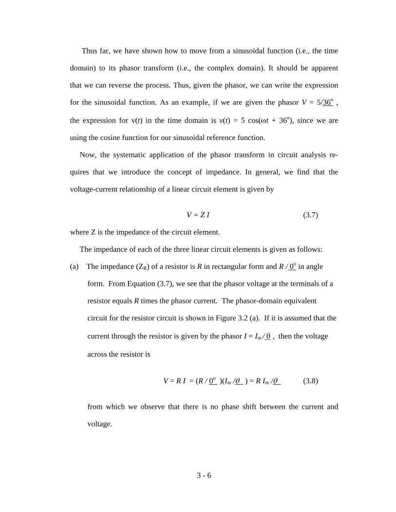
Thus far, we have shown how to move from a sinusoidal function (i.e., the time domain) to its phasor transform (i.e., the complex domain). It should be apparent that we can reverse the process. Thus, given the phasor, we can write the expression for the sinusoidal function. As an example, if we are given the phasor V = 5/36o , the expression for v(t) in the time domain is v(t) = 5 cos(ωt + 36o), since we are using the cosine function for our sinusoidal reference function. Now, the systematic application of the phasor transform in circuit analysis re- quires that we introduce the concept of impedance. In general, we find that the voltage-current relationship of a linear circuit element is given by V = Z I (3.7) where Z is the impedance of the circuit element. The impedance of each of the three linear circuit elements is given as follows: (a) The impedance (ZR) of a resistor is R in rectangular form and R / 0o in angle

form. From Equation (3.7), we see that the phasor voltage at the terminals of a

resistor equals R times the phasor current. The phasor-domain equivalent

circuit for the resistor circuit is shown in Figure 3.2 (a). If it is assumed that the

current through the resistor is given by the phasor I = Im / θ , then the voltage

across the resistor is

V = R I = (R / 0o )(Im /θ ) = R Im /θ (3.8)

from which we observe that there is no phase shift between the current and

voltage.

3 - 6

Figure 3.2. Phasor Domain Equivalent Circuits

(b) The impedance (ZL) of an inductor is jωL in rectangular form and ωL/ 90o

in angle form. Again, from Equation (3.7), we see that the phasor voltage

at the terminals of an inductor equals jωL times the phasor current. The

phasor-domain equivalent circuit for the inductor is shown in Figure 3.2(b).

If we assume I = Im /θ , then the voltage is given by

V = (jωL) I = (ωL / 90o )(Im /θ ) = ωLIm / θ + 90o (3.9) from which we observe that the voltage and current will be out of phase by exactly 90o. In particular, the voltage will lead the current by 90o or, what is equivalent, the current will lag behind the voltage by 90o. (c) The impedance (ZC) of a capacitor is l/jωC (or -j/ωC) in rectangular form

and 1/ωC/ -90o in angle form. Equation (3.7) indicates that the phasor

voltage at the terminals of a capacitor equals l/jωC times the phasor current.

The phasor-domain equivalent circuit for the capacitor is shown in Figure

3.2(c).

3 - 7

ZC = 1/jωC = -j/ωCZL = jωLZR = R

If we assume I = Im /θ , then the voltage is given by V = (- j/ωC ) I = (1/ωC / -90o )(Im /θ ) = Im/ωC /θ - 90o (3.10) where in this case, the voltage across the terminals of the capacitor will lag behind the capacitor current by 90o. The alternative way to express the phase relationship is to say that the current leads the voltage by 90o. It can be shown that Ohm's law and Kirchhoff's laws apply to the phasor do- main. Thus, all of the techniques used for analyzing dc resistive circuits can be used to find phasor currents and voltages. Thus, new analysis techniques are not needed to analyze circuits in the phasor domain. The basic tools of series-parallel simplifi- cations, source transformations, Thevenin-Norton equivalent circuits, superposition, node-voltage analysis, and mesh-current analysis can all be used in the analysis of circuits in the phasor domain in order to determine the steady-state response of a network to sinusoidal sources. The problem of learning phasor circuit analysis involves two parts. First, you must be able to construct the phasor-domain model of the circuit and, second, you must be able to algebraically manipulate complex numbers and/or quantities to arrive at a solution. We will demonstrate this by considering the example circuit shown in Figure 3.3, which consists of a resistor, inductor, and capacitor connected in series across the terminals of a sinusoidal voltage source. Assume the steady-state voltage source is a sine wave that we can represent as vs(t) = 5 cos ωt at a frequency of f = 1000Hz. The first step in the solution is to determine the phasor-domain equivalent circuit. Given a frequency of 1000 Hz, then ω = 2π f = 6283 radians/second. Therefore, the

3 - 8

Ω−=−=⎟⎠⎞

⎜⎝⎛−= 8.31

)5)(6283(101 6

jjC

jZC ω

Figure 3.3: Example Sinusoidal Steady-State Analysis Circuit impedance of the inductor is ZL = jωL = j(6283)(0.030) = j 188.5Ω (3.11) and the impedance of the capacitor is (3.12) The phasor transform of vs(t) is VS = 5 / 0o (3.13) The phasor domain equivalent circuit for the circuit shown in Figure 3.3 is illustrated in Figure 3.4. We can compute the phasor current by simply dividing the phasor voltage of the

voltage source by the total impedance across its terminals. The total impedance is

ZT = R + ZL + ZC (3.14)

3-9

22 )7.156()100( +=TZ

Figure 3.4: Phasor Domain Equivalent Circuit since the resistor, inductor, and capacitor are connected in series. Substituting values for R, ZL, and ZC gives ZT = 100 + j 188.5 - j 31.8 = 100 + j 156.7. (3.15) Converting this to angle form, we have / tan-1(156.7/100) , (3.16) which simplifies to ZT = 185.9/ + 57.5o . (3.17) Thus, the current is equal to I = VS / ZT = (5 / 0o )/(185.9 / 57.5o ) = 0.0269 / -57.5° A. (3.18)

and the voltage across the capacitor is VC = ZC I = (31.8 / -90o )(0.0269 / -57.5o ) = 0.855 / -147.5o V. (3.19)

3-10

We can now write the stead-state expressions for I(t) and vC(t) directly: i(t) = 26.9 cos (6283t - 57.5o ) mA (3.20) and vC(t) = 0.855 cos (6283t - 147.5o ) V. (3.21) 3.3.2 Frequency Response of AC Circuits: Bode Diagrams As indicated above, network connections of linear circuit elements used to transmit signals generally result in an output signal with an amplitude and time dependence that differs from that of the input signal. If the input signal is sinusoidal, so too will be the output for a linear network. However, usually both the amplitude ratio and the phase difference between the input and the output signals will depend on the frequency. A particularly convenient graphical representation is obtained if logarithmic scales are used for both the frequency and the amplitude ratio while a linear scale is used for the phase difference. Also, extremely useful approximate graphical representations can be obtained for many networks that result in a series of straight lines on these graphs. Both representations are called Bode Diagrams. In this part of the experiment, the measured response of two networks will be compared to that theoretically predicted and the straight line approximations. In addition, decibel notation will be introduced. The frequency response of the elementary circuit shown in Figure 3.5, where vi(t)

corresponds to the input signal and vo(t) to the output signal, will initially be

determined. Sinusoidal signals will be assumed. In analyzing this circuit, the

3 - 11

( ) ,1)(Cj

R

VZ

VI ii

ωω

ω+

==

.11

1RCj

V

CjR

VCj

IZV iiCo ω

ωω +

=

⎟⎟⎟⎟

⎠

⎞

⎜⎜⎜⎜

⎝

⎛

+⎟⎟⎠

⎞⎜⎜⎝

⎛==

impedance across vi is a function of the operating frequency and can be expressed as Z(ω) = R + 1/jωC . (3.22) Using Ohm's law in the phasor domain, the current in the circuit is (3.23) and the output voltage, which is equal to the voltage across the capacitor, is (3.24) Examination of Equation (3.24) above indicates that for low frequencies (that is, for ω 0 ), the output voltage is approximately equal to the input voltage (i.e. V0 Vi). Also, for high frequencies (that is for ω ∞), the output voltage becomes negligibly small (i.e. V0 0). Since low frequency signals are virtually unaffected, a network of this type is called a low-pass filter. It should be noted that many complex circuits comprised of active elements, such as transistors, may be reduced to an equivalent circuit of this type. The capacitance, C, is often the

3 - 12

R

.1

1)( 0

RCjVV

Ai ω

ω+

==

,)(1

1|)(|2RC

Aω

ω+

=

,

1

1|)(|2

1⎟⎟⎠

⎞⎜⎜⎝

⎛+

=

ωω

ωA

result of unavoidable circuit and element capacitances, while the resistance, R, is the Thevenin equivalent resistance of the complex circuit. If we let A be defined as the ratio of the output voltage to the input voltage, then (3.25) Now A(ω) can be expressed in terms of its magnitude and phase angle, where the magnitude is (3.26) while the phase angle is θ(ω) = -tan -1 (ωRC) . (3.27) If we define the critical frequency ω1 to be ω1 = 1/RC (3.28) then, upon substitution in Equation (3.26) and Equation (3.27), we find (3.29) and θ (ω) = - tan -1 (ω/ω1) . (3.30) Now, the amplitude of the voltage ratio is normally specified in decibels (dB), and is defined as AdB = 20 log10 |A(ω)| dB.

3 - 13

Bode plots relate the magnitude and phase angle of the voltage ratio of a network

with frequency as the independent variable. Usually, frequency in Hertz or radians

per second is used as the abscissa on a logarithmic scale and the amplitude of the

voltage ratio in dB on one ordinate and the phase angle on a linear scale as another

ordinate. An example for the low pass-filter is shown in Figure 3.6 where we have

plotted AdB versus log ω and θ versus log ω. Note that Bode plots are shown for

both the straight line approximation (solid) and the actual (dashed) values.

Figure 3.6: A Bode Plot for a Low-Pass Filter with Critical Frequency ω1.

3 - 14

AdB

θ

_______ Approximate response- - - - Actual Response

.11

1|)(| =≈ωA

.707.02

111

1|)(| 1 ==+

=ωA

We can obtain values for |A(ω)| and θ(ω) for the low-pass filter using Equa- tion (3.29) and Equation (3.30). For ω << ωI , we have from Equation (3.29), (3.32) We can determine the phase angle from Equation (3.30), namely, θ ≅ tan -1 (0) = 0o. (3.33) In decibels, we see that AdB = 0 since 20 log10(1) = 0. Now, when ω is an order of magnitude below ω1 (i.e., ω = 0.1ω1), we find that θ = tan

-1 (0.1) = -5.710° ≅ - 6 °. (3.34) These relationships between A(ω) and θ(ω) are shown plotted in Figure 3.6. For ω = ω1, we can compute the magnitude of the voltage amplitude ratio from Equation (3.29) as (3.35) Thus, |V0| = 0.707 |Vi| at the critical frequency ω1. In decibels, we can express the magnitude of the voltage ratio as AdB = 20 log10 (1/√2) = -3.0 dB . (3.36) It follows, then, that at ω = ω1 the magnitude of the voltage ratio is reduced by 3 dB. As a result, the critical frequency is often called the -3 dB point. Also, since the power-transfer ratio is proportional to the square of the voltage ratio, i.e.,

3-15

,10

loglog20'' 110

110 ⎥

⎦

⎤⎢⎣

⎡⎟⎟⎠

⎞⎜⎜⎝

⎛−⎟⎟

⎠

⎞⎜⎜⎝

⎛=−

nn

YXωω

ωω

(1/√2)2, the critical frequency ω1 (or f1 when expressed in Hertz) is also known as the

half-power frequency. The phase angle for ω = ω1 is calculated by substituting into

Equation (3.30) and is given by

θ = - tan -1 (1) = - 45° . (3.37) For ω >> ω1, we determine from Equation (3.29) that |A(ω1)| ≅ ω1 /ω . (3.38) Hence, in this region, |A(ω)| varies inversely with frequency. The rate of change can be determined by considering a decade of frequency. Let X = |A(ωn)| and X dB = 20 log10 X , (3.39) where X is the magnitude of the voltage ratio function at some frequency ωn , and let Y = |A(10ωn)| and Y dB = 20 log10 Y , (3.40) where Y is the magnitude of the voltage ratio function at a frequency 10 times ωn . Then, using Equation (3.38), the difference in voltage ratio (in dB) over a decade of frequency is given by (3.41) which simplifies to X ' - Y ' = 20 log10 (10) = 20 dB . (3.42)

3 - 16

Thus, the gain at 10ωn is 20 dB less than it was at ωn. It follows then, that the rate of fall of the amplitude ratio, where ω >> ω1, is -20 dB/decacde. Finally, from the expression for the phase angle in Equation (3.30), we observe that as ω ∞, θ -90°, but at ω = 10ω1, θ = - tan -1 (10) = -84.289 ≈ - 84° . (3.43) As indicated previously, Figure 3.6 is a Bode plot for a low-pass filter with

critical frequency ω1. Notice that the approximate Bode plot makes use of the

straight-line segments to approximate the actual response (shown as a dotted line

around the critical frequency). Also, note that the maximum amplitude rolloff is -20

dB/decade and the maximum phase shift is - 90°.

Equally important to the low-pass filter just considered is a network in which the positions of the capacitor and the resistor are interchanged as shown in Figure 3.7. In this case, since the capacitance is in series with the input voltage source and the output terminals of the network, the voltage v0 becomes very small as the frequency is reduced. For zero frequency (i.e., "dc"), the output voltage is zero since a capacitor blocks dc voltages. At very high frequencies, the capacitor's impedance approaches

3 - 17

,1110

RCj

V

CjR

VRRIV ii

ωω+

=

⎟⎟⎟⎟

⎠

⎞

⎜⎜⎜⎜

⎝

⎛

+==

.11

1)(

RCj

A

ω

ω+

=

,11

1|)(|2

⎟⎠⎞

⎜⎝⎛+

=

RC

A

ω

ω

a short-circuit resulting in an output voltage that tends to be very nearly equal to

the input voltage. Thus, this circuit configuration is classified as a high-pass filter

since it attenuates low frequency signal components and passes high frequency

components. When a capacitance is used to couple time-varying signal components

from one part of an electronic circuit to another, this type of equivalent circuit often

results. Also, this type of circuit may be intentionally introduced in signal processing

systems to eliminate undesirable low-frequency (including "dc" ) components.

The analysis of this circuit is similar to that of a low-pass filter. The output voltage is given by

(3.44) and, if we let A again be defined as the voltage ratio, it follows that (3.45) The magnitude and phase angle are (3.46) and θ (ω) = + tan -1 (1/ωRC). (3.47)

3 - 18

,

1

1|)(|2

1 ⎟⎠⎞

⎜⎝⎛+

=

ωω

ωA

.tan)( 11 ⎟⎠⎞

⎜⎝⎛= −

ωω

ωθ

Again, in terms of the critical frequency ω1 = 1/RC, we have (3.48) and (3.49) A Bode plot for the high-pass filter is shown in Figure 3.8. Notice in this case that

Figure 3.8: A Bode plot for a High-Pass Filter with Critical Frequency ω1 .

3 - 19

θ

_______ Approximate response- - - - Actual Response

the magnitude and phase angle of the voltage ratio is again 3 dB down and +45°, respectively, at the critical frequency. The rate of increase for ω << ω1, is 20 dB/decade and as ω 0, θ + 90°, while at ω = 0.1ω1, θ = + 84°. For ω >> ω1, the magnitude of the voltage ratio is 1 (0 dB) and the phase angle is 0°. Obtaining values for A(ω) and θ(ω) from Equation (3.48) and Equation (3.49), as shown previously for the low-pass filter, is left to the student. 3.4 Advanced Preparation The following advanced preparation is required before coming to the laboratory:

(1) Thoroughly read and understand the theory and procedures.

(2) Solve for the steady-state voltage across C2 in the circuit shown in Figure 3.9

at both frequencies given to you by your instructor. (3) Perform a PSpice Transient simulation to find the steady-state voltage across C2

in the circuit shown in Figure 3.9. Note that the simulation time must be long enough

for the transient response to reach steady-state. Make a copy of a segment of the

steady-state voltage. Do the simulation for both frequencies.

(4) Solve for the steady-state voltage across R4 in the circuit shown in Figure 3.10 at

both frequencies given to you by your instructor.

(5) Perform a PSpice Transient simulation to find the steady-state voltage across R4

in the circuit shown in Figure 3.10. Note that the simulation time must be long

enough for the transient response to reach steady-state. Make a copy of a segment of

the steady-state voltage. Do the simulation for both frequencies.

(6) Calculate the critical frequency in Hertz (using the values given to you by your

instructor) for the low-pass and high-pass filter test circuits shown in Figure 3.11 and

Figure 3.12, respectively.

3 - 20

3.5 Experimental Procedure 3.5.1 AC Analysis of a RC Circuit Construct the circuit in Figure 3.9 using the HP33120A Function Generator output as Figure 3.9: RC circuit to be used for performing AC analysis. vT(t). Connect Channel 1 of the scope across vT(t) and Channel 2 across C2 and

trigger the scope on Channel 1. Set the output of the HP33120A to produce a sine

wave, adjust its peak-to-peak voltage to V1 volts (which is a peak voltage of V1/2

volts) using the scope, and set its frequency to fa Hz. Check using the frequency

counter and digital oscilloscope. Now, measure the voltage across C2 by measuring

the peak amplitude of the voltage waveform on Channel 2 plus the phase shift of the

waveform on Channel 2 with respect to the waveform on Channel 1. Next, set the

output of the HP33120A to have a frequency of fb Hz and repeat the above procedure.

3.5.2 AC Analysis of a RLC Circuit

In a manner similar to the way the circuit in Figure 3.9 was constructed, assemble the circuit shown in Figure 3.10. Set the output of the HP33120A to produce a sine

3 - 21

vT(t)

Figure 3.10: RLC circuit to be used for performing AC analysis. wave, adjust its peak-to-peak voltage to V2 volts (which is a peak voltage of V2/2

volts) using the scope, and set its frequency to fc Hz. Check using the frequency

counter and digital scope. Now, measure the voltage across R4 by measuring the peak

amplitude of the voltage waveform on Channel 2 plus the phase shift of the waveform

on Channel 2 with respect to the waveform on Channel 1. Next, set the output of the

HP33120A to have a frequency of fd Hz and repeat the above procedure.

3.5.3 RC Low-Pass Filter In this part, you are to experimentally determine the amplitude and phase angle of the

voltage ratio of the RC low-pass filter network shown in Figure 3.11. This should be

done over a frequency range from two orders of magnitude below upto two orders of

magnitude above the critical frequency f1. Construct the circuit in Figure 3.11 using

the HP33120A output vT(t) as vi(t). Connect Channel 1 of the scope to measure vi and

Channel 2 to measure v0 and trigger the scope on Channel 1. Next, set the output to

be sinusoidal with a peak-to-peak voltage of V3 volts. Use the following procedure to

determine the critical frequency and to obtain frequency response data, i.e., values for

the amplitude and phase angle of the voltage ratio as a function of frequency. Be sure

3 - 22

Figure 3.11: Low-Pass Filter test circuit. to use the digital scope or frequency counter to get accurate frequency values.

(a) Experimentally determine the critical frequency f1 for the circuit. Since we know

at the critical frequency that v0 = vi/√ 2 = 0.707vi , this can be accomplished by

varying the frequency of the HP33120A until the output voltage on Channel 2 is

equal to V3/√ 2 volts peak-to-peak. Record this frequency as f1. Also, observe

both waveforms on the scope and determine their phase angle difference at this

frequency. Make a hardcopy of this display. If the phase difference is not close

to 45°, then either the measurement is in error or the circuit is not functioning

properly and you must correct this problem before proceeding.

(b) Now at each of the following frequencies, (1) record the peak-to-peak values of

v0 and vi in a table and calculate the ratio of v0 divided by vi, and (2) measure and

record the phase angle between v0 and vi. The following frequencies were

chosen to obtain adequate data points around f1.

f1 /100 (two decades down)

f1 /10 (one decade down) f1 /4 (two octaves down) f1/2 (one octave down)

3 - 23

f1 x 2 (one octave up) f1 x 4 (two octaves up) f1 x 10 (one decade up) f1 x 100 (two decades up) Be sure you adjust the HP33120A output to V3 volts peak-to-peak if it changes

significantly when you vary the frequency.

(c) Finally, record any additional data points for the peak-to-peak voltages and time

differences needed to calculate accurate voltage ratios and phase angles from

one decade to two decades below f1 and from one decade to two decades above

f1. Again, be sure you adjust the HP33120A output to V3 volts peak-to-peak if it

changes significantly when you vary the frequency.

3.5.4 RC High-Pass Filter

Now, experimentally determine the response of the high-pass filter shown in Fig-

ure 3.12 using the same procedure outlined 3.5.3. Figure 3.12: High-Pass Filter test circuit.

3 - 24

3.6 Report 3.6.1 AC Analysis of a RC Circuit 3.6.1.1 Clearly show your analysis to solve for the steady-state voltage across the

capacitor C2 in Figure 3.9. In particular, draw the phasor-domain equivalent circuit,

show all steps in determining the phasor voltage across C2, and express your answer

as a sinusoidal function in the time domain. This should be done for both frequencies

used (fa and fb).

3.6.1.2 Clearly explain the procedure you used to measure the peak voltage and

phase angle of the voltage across the capacitor C2 using the scope. Specifically, you

should provide a hardcopy of v0 compared to vs indicating the peak voltages in volts

and phase difference in time. Also, show how you converted the phase difference

from time to degrees.

3.6.1.3 Discuss the accuracy of your measured results compared to your solution in

Problem 1.1 above and indicate the reasons for any errors between the measurements

and the theory.

3.6.1.4 Attach a copy of the steady-state voltage across C2 obtained per Section 3.4

(3) and comment on the experimental results versus PSpice simulation results.

3.6.2 AC Analysis of a RLC Circuit 3.6.2.1 Clearly show your analysis to solve for the steady-state voltage across the

resistor R4 in Figure 3.10. In particular, draw the phasor-domain equivalent circuit,

show all steps in determining the phasor voltage across R4, and express your answer

as a sinusoidal function in the time domain. This should be done for both frequencies

used (fc and fd).

3 - 25

3.6.2.2 Discuss the accuracy of your measured results compared to your solution in

Step 2.1 above and indicate the reasons for any errors between the measurements and

the theory.

3.6.2.3 Attach a copy of the steady-state voltage across R4 obtained per Section 3.4

(5) and comment on the experimental results versus PSpice simulation results.

3.6.3 RC Low-Pass Filter 3.6.3.1 Prepare a table presenting your measurements for vi, v0, the amplitude of the

voltage ratio |A|, and the phase angle (θ) as a function of frequency for the low-pass

filter test circuit in Figure 3.11. Calculate AdB for each of the frequencies and add

these values to your table. Generate a Bode plot of AdB and θ as a function of

frequency in Hertz on semilog paper.

3.6.3.2 Calculate the theoretical critical frequency, f1, in Hertz for the low-pass filter

in Figure 3.11 and draw the straight line approximate Bode plot for the amplitude of

the voltage ratio and phase angle on the same graph as the experimental data.

3.6.3.3 Discuss how accurate the straight line approximation is compared to the

theory and your experimental data.

3.6.4 RC High-Pass Filter 3.6.4.1 Prepare a table presenting your measurements for vi, v0, the amplitude of the

voltage ratio |A|, and the phase angle (θ) as a function of frequency for the high-pass

filter test circuit in Figure 3.12. Calculate AdB for each of the frequencies and add

these values to your table. Generate a Bode plot of AdB and θ as a function of

frequency in Hertz on semilog paper.

3 - 26

3.6.4.2 Calculate the theoretical critical frequency, f1, in Hertz for the high-pass filter

in Figure 3.12 and draw the straight line approximate the Bode plot for the amplitude

of the voltage ratio and phase angle on the same graph as the experimental data.

3.6.4.3 Discuss how accurate the straight line approximation is compared to the

theory and your experimental data.

3.6.5 Design Problem A combination of low-pass and high-pass networks can give a frequency response that is similar to that of a band-pass filter. Consider the network below. Design the network so as to have (1) |Vo/VT| ≈ 0.5 at f = 1 kHz, (2) |Vo/VT| ≤ 0.1

for f ≤ 60 Hz, and (3) |Vo/VT| ≤ 0.1 for f ≥ 16k Hz. The figure above indicates these

specified values. Use the load resistance RL specified by the instructor.

3.6.5.1 Identify the values selected for the capacitors (C1 & C2) and resistor (R1).

3.6.5.2 Use PSpice to provide a plot of |Vo / VT| showing the response of your circuit

design. Use a log scale for frequency f.

3.6.5.3 Verify that the design meets the requirements by doing a steady–state AC

PSpice simulation of the circuit at the three frequencies indicated on the figure

above. Present results in tabular form.

3 - 27

≤ 0.1

VoVT RL

+

R1

C1

C2 V2 V1

0.5

f(Hz)1k 16k60

|Vo/VT|

3.7 References

1. Nilsson, J. W., Electric Circuits, (5th ed.), Prentice Hall, Upper Saddle River, New Jersey, 2001.

2. Grinich, V. H. and Jackson, H. C., Introduction to Integrated Circuits,

McGraw-Hill, New York, 1975.

3 - 28