christian weiˇ - core
TRANSCRIPT

Scheduling Models with Additional Features
Synchronization, Pliability and Resiliency
Christian Weiß
Submitted in accordance with the requirements
for the degree of Doctor of Philosophy
The University of Leeds
School of Computing
December 2016
brought to you by COREView metadata, citation and similar papers at core.ac.uk
provided by White Rose E-theses Online


The candidate confirms that the work submitted is his own, except where work which has formed
part of a jointly authored publication has been included. The contribution of the candidate
and the other authors to this work has been explicitly indicated below. The candidate confirms
that appropriate credit has been given within the thesis where reference has been made to the
work of others.
Some parts of the work presented in Chapters 4, 5 and 6 have been published in the following
articles:
C. Weiß, S. Waldherr, S. Knust, N. V. Shakhlevich (2016) Open shop scheduling with syn-
chronization. Journal of Scheduling (published online), doi: 10.1007/s10951-016-0490-0,
C. Weiß, S. Knust, N. V. Shakhlevich, S. Waldherr (2016) The assignment problem with
nearly Monge arrays and incompatible partner indices. Discrete Applied Mathematics
211, 183–203.
For both papers, all four authors worked on text, formulation, proof reading and literature
search. In the first paper, scientific results (other than in Section 4) are mostly due to C. Weiß,
though the other authors had large part in finding good presentation methods for this work.
Results in Section 4 are due to S. Waldherr, N. Shakhlevich and C. Weiß.
In the second paper, results in Sections 2 and 3 are mostly due to C. Weiß. The result in Section
3 was achieved in collaboration with N. Shakhlevich. The first complete proof for the result in
Section 4 was achieved by S. Waldherr and C. Weiß in collaboration. N. Shakhlevich played a
large role in finding a good presentation for that work.
This copy has been supplied on the understanding that it is copyright material and that no
quotation from the thesis maybe published without proper acknowledgement.
©2016 The University of Leeds and Christian Weiß


Acknowledgements
I would like to thank my supervisor Natasha Shakhlevich for her invaluable and patient support,
starting from the application process and continuing through to the submission of this thesis.
Without her help and guidance I would never have applied to study for a PhD in Leeds, let
alone completed it. My thanks also go to my second supervisor, Martin Dyer, for providing
helpful advice ever since joining my supervisory team.
Particular gratitude is also extended to Vladimir Deineko and Haiko Muller for examining
this thesis and making many helpful suggestions for its improvement.
I am further grateful to our main collaborators Sigrid Knust and Stefan Waldherr for the
time they invested in our joint work and for their hospitality when I visited them in Osnabruck.
Thanks for work put into our collaboration is also extended to Evgeny Gurevsky.
On a more personal (but at least equally important) note I want to thank all friends and
colleagues who supported me both in Leeds and at home in Troisdorf: Sam Wilson and Thilo
Simon for providing sounding boards for my ideas, especially in the early stages of my studies;
Bjorn Buhr, Sebastian Kremer, Sebastian Heer and Sven Gießelbach for steadfast support and
friendship since long before I started studying in Leeds; Emma Dobson, Ben White and others
for providing friendship and company during my stay in Leeds; the people working in my
office, especially Qingxu Dou and Fouzhan Hosseini; the PGR community both in the school
and beyond, especially Marwan Al-Tawil, Alicja Piotrkowicz, Bernhard Primas and the alumni
Matt Benathan and Elaine Duffin. Further thanks goes to the other members of my research
group, those undergraduate students I had the pleasure of teaching during my time in Leeds,
and many others, who I cannot name now, but who provided an invaluable social component
and helped my find some balance during these busy three years.
Finally, I would like to give my deepest thanks to my parents, who have supported me and
believed in me for much longer than any of the people named before even knew me.


Abstract
In this thesis we study three new extensions of scheduling models with both practical and
theoretical relevance, namely synchronization, pliability and resiliency. Synchronization has
previously been studied for flow shop scheduling and we now apply the concept to open shop
models for the first time. Here, as opposed to the traditional models, operations that are
processed together all have to be started at the same time. Operations that are completed are
not removed from the machines until the longest operation in their group is finished.
Pliability is a new approach to model flexibility in flow shops and open shops. In schedul-
ing with pliability, parts of the processing load of the jobs can be re-distributed between the
machines in order to achieve better schedules. This is applicable, for example, if the machines
represent cross-trained workers.
Resiliency is a new measure for the quality of a given solution if the input data are uncertain.
A resilient solution remains better than some given bound, even if the original input data are
changed. The more we can perturb the input data without the solution losing too much quality,
the more resilient the solution is.
We also consider the assignment problem, as it is the traditional combinatorial optimization
problem underlying many scheduling problems. Particularly, we study a version of the assign-
ment problem with a special cost structure derived from the synchronous open shop model
and obtain new structural and complexity results. Furthermore we study resiliency for the
assignment problem.
The main focus of this thesis is the study of structural properties, algorithm development
and complexity. For synchronous open shop we show that for a fixed number of machines the
makespan can be minimized in polynomial time. All other traditional scheduling objectives are
at least as hard to optimize as in the traditional open shop model.
Starting out research in pliability we focus on the most general case of the model as well as
two relevant special cases. We deliver a fairly complete complexity study for all three versions
of the model.
Finally, for resiliency, we investigate two different questions: ‘how to compute the resiliency
of a given solution?’ and ‘how to find a most resilient solution?’. We focus on the assignment
problem and single machine scheduling to minimize the total sum of completion times and
present a number of positive results for both questions. The main goal is to make a case that
the concept deserves further study.


Contents
1 Introduction 1
2 Preliminaries 5
2.1 Necessary notation from graph theory . . . . . . . . . . . . . . . . . . . . . . . . 5
2.2 General definitions and notation for scheduling . . . . . . . . . . . . . . . . . . . 7
2.2.1 A general scheduling problem . . . . . . . . . . . . . . . . . . . . . . . . . 7
2.2.2 The three-field notation . . . . . . . . . . . . . . . . . . . . . . . . . . . . 8
2.3 Scheduling models . . . . . . . . . . . . . . . . . . . . . . . . . . . . . . . . . . . 11
2.3.1 Single machine scheduling problems . . . . . . . . . . . . . . . . . . . . . 11
2.3.2 Scheduling problems with parallel identical machines . . . . . . . . . . . 13
2.3.3 Scheduling problems with parallel uniform machines . . . . . . . . . . . . 14
2.3.4 Flow shop problems . . . . . . . . . . . . . . . . . . . . . . . . . . . . . . 14
2.3.5 Open shop problems . . . . . . . . . . . . . . . . . . . . . . . . . . . . . . 15
2.3.6 Job shop problems . . . . . . . . . . . . . . . . . . . . . . . . . . . . . . . 16
2.4 The linear assignment problem . . . . . . . . . . . . . . . . . . . . . . . . . . . . 16
2.4.1 The two-dimensional linear assignment problem . . . . . . . . . . . . . . 17
2.4.2 Matching problems in bipartite and general graphs . . . . . . . . . . . . 18
2.4.3 The multi-dimensional linear assignment problem . . . . . . . . . . . . . 19
2.4.4 The linear assignment problem with Monge costs . . . . . . . . . . . . . 19
I Synchronization 23
3 Definitions, notation and related work 25
3.1 Introduction and definitions . . . . . . . . . . . . . . . . . . . . . . . . . . . . . . 25
3.2 Related work . . . . . . . . . . . . . . . . . . . . . . . . . . . . . . . . . . . . . . 27
4 Synchronous Open Shop Scheduling with Two Machines 31
4.1 Minimizing the makespan . . . . . . . . . . . . . . . . . . . . . . . . . . . . . . . 31
4.1.1 Problem O2|synmv|Cmax . . . . . . . . . . . . . . . . . . . . . . . . . . . 32
4.1.2 Problem O2|synmv, rel|Cmax . . . . . . . . . . . . . . . . . . . . . . . . . 44
i

ii CONTENTS
4.2 Scheduling with deadlines . . . . . . . . . . . . . . . . . . . . . . . . . . . . . . . 49
4.3 Minimizing the total completion time . . . . . . . . . . . . . . . . . . . . . . . . 54
4.4 Details for the NP-hardness of O2|synmv|∑Cj . . . . . . . . . . . . . . . . . . 62
5 The Assignment Problem with Nearly Monge Arrays and Incompatible Part-
ner Indices 77
5.1 Introduction . . . . . . . . . . . . . . . . . . . . . . . . . . . . . . . . . . . . . . 77
5.2 Applications . . . . . . . . . . . . . . . . . . . . . . . . . . . . . . . . . . . . . . 80
5.3 NP-hardness of problem AP(d, λ) . . . . . . . . . . . . . . . . . . . . . . . . . . 83
5.4 Some properties of nearly Monge matrices with incompatible partner indices . . 87
5.4.1 Nonexistence of a Monge sequence . . . . . . . . . . . . . . . . . . . . . . 87
5.4.2 Recognizing nearly Monge arrays . . . . . . . . . . . . . . . . . . . . . . 88
5.4.3 Completing nearly Monge arrays . . . . . . . . . . . . . . . . . . . . . . . 90
5.5 The corridor property for problem AP(d, λ) . . . . . . . . . . . . . . . . . . . . . 91
5.6 A linear-time algorithm for problem AP(d, λ) with fixed d and λ . . . . . . . . . 97
5.7 The corridor property for other versions of the assignment problem . . . . . . . . 101
5.7.1 Axial three-dimensional assignment problem with decomposable costs . . 101
5.7.2 Planar 3-dimensional assignment problem with a layered Monge matrix . 103
5.7.3 Bottleneck assignment problem with a bottleneck nearly Monge matrix
and its generalizations . . . . . . . . . . . . . . . . . . . . . . . . . . . . 106
5.8 NP-completeness of 3-DM with incompatible partner indices . . . . . . . . . . . . 107
6 The relaxed problem O|synmv, rel|Cmax 111
7 Conclusions and further research 115
7.1 Synchronous open shop scheduling . . . . . . . . . . . . . . . . . . . . . . . . . . 115
7.2 Assignment problem with a nearly Monge matrix . . . . . . . . . . . . . . . . . 116
7.3 Further research for synchronous scheduling models . . . . . . . . . . . . . . . . . 120
II Pliability 123
8 Definitions, notation and related work 125
8.1 Introduction and definitions . . . . . . . . . . . . . . . . . . . . . . . . . . . . . . 125
8.2 Related work . . . . . . . . . . . . . . . . . . . . . . . . . . . . . . . . . . . . . . 127
9 Shop scheduling problems with pliable jobs 131
9.1 General properties and reductions . . . . . . . . . . . . . . . . . . . . . . . . . . 131
9.1.1 Pliability of type (i) . . . . . . . . . . . . . . . . . . . . . . . . . . . . . . 131
9.1.2 Pliability of type (ii) . . . . . . . . . . . . . . . . . . . . . . . . . . . . . 133
9.1.3 Pliability of type (iii) . . . . . . . . . . . . . . . . . . . . . . . . . . . . . 137

CONTENTS iii
9.2 Type (i) problems with minmax criteria . . . . . . . . . . . . . . . . . . . . . . . 138
9.2.1 Type (i) problems F |plbl|Cmax and O|plbl|Cmax . . . . . . . . . . . . . . 138
9.2.2 Type (i) problems F |plbl|Lmax and O|plbl|Lmax . . . . . . . . . . . . . . 139
9.3 Type (ii) problems with minmax criteria . . . . . . . . . . . . . . . . . . . . . . 141
9.3.1 Type (ii) problem F |plbl(p)|Cmax . . . . . . . . . . . . . . . . . . . . . . 141
9.3.2 Type (ii) problem O|plbl(p)|Cmax . . . . . . . . . . . . . . . . . . . . . . 144
9.3.3 Type (ii) problem F |plbl(p)|Lmax . . . . . . . . . . . . . . . . . . . . . . 146
9.4 Type (iii) problems with the makespan objective and m = 2 . . . . . . . . . . . 148
9.4.1 Problem F2|plbl(pij, pij)|Cmax . . . . . . . . . . . . . . . . . . . . . . . . 148
9.4.2 Problem O2|plbl(pij, pij)|Cmax . . . . . . . . . . . . . . . . . . . . . . . . 150
9.5 Type (i) and type (ii) problems with min-sum criteria . . . . . . . . . . . . . . . 153
9.5.1 Type (i) problems F |plbl|∑Cj and O|plbl|∑Cj . . . . . . . . . . . . . . 153
9.5.2 Type (ii) problem F |plbl(p)|∑Cj . . . . . . . . . . . . . . . . . . . . . . 155
9.5.3 Type (ii) problem O|plbl(p)|∑Cj . . . . . . . . . . . . . . . . . . . . . . 156
9.5.4 Other problems with min-sum criteria . . . . . . . . . . . . . . . . . . . . 159
9.6 Proof of Lemma 36 . . . . . . . . . . . . . . . . . . . . . . . . . . . . . . . . . . . 163
10 Conclusions and further research 169
10.1 General observations . . . . . . . . . . . . . . . . . . . . . . . . . . . . . . . . . . 170
10.2 Pliability of type (i) and (ii) with n < m . . . . . . . . . . . . . . . . . . . . . . . 171
10.3 Further research . . . . . . . . . . . . . . . . . . . . . . . . . . . . . . . . . . . . 173
III Resiliency 175
11 Definitions, notation and related work 177
11.1 Introduction . . . . . . . . . . . . . . . . . . . . . . . . . . . . . . . . . . . . . . 177
11.2 Related work . . . . . . . . . . . . . . . . . . . . . . . . . . . . . . . . . . . . . . 181
11.2.1 Stability . . . . . . . . . . . . . . . . . . . . . . . . . . . . . . . . . . . . . 182
11.2.2 Robustness . . . . . . . . . . . . . . . . . . . . . . . . . . . . . . . . . . . 184
12 Resiliency for Combinatorial Optimization Problems with Uncertain Data 187
12.1 General Properties . . . . . . . . . . . . . . . . . . . . . . . . . . . . . . . . . . . 187
12.1.1 Complexity Aspects . . . . . . . . . . . . . . . . . . . . . . . . . . . . . . 188
12.1.2 Properties of objective functions that limit the search for worst-case de-
viations . . . . . . . . . . . . . . . . . . . . . . . . . . . . . . . . . . . . . 188
12.1.3 Problems with the `∞-norm . . . . . . . . . . . . . . . . . . . . . . . . . 190
12.2 The Assignment Problem with Uncertain Costs . . . . . . . . . . . . . . . . . . 191
12.2.1 The assignment problem with arbitrary fluctuation factors . . . . . . . . 191
12.2.2 Assignment problem with binary fluctuation factors αij ∈ 0, 1 . . . . . 200
12.2.3 The bottleneck assignment problem . . . . . . . . . . . . . . . . . . . . . 205

iv CONTENTS
12.3 Problem 1||∑Cj with uncertain cost . . . . . . . . . . . . . . . . . . . . . . . . 208
12.3.1 The case with arbitrary fluctuation factors αj for the job processing times 209
12.3.2 The case with binary fluctuation factors αj ∈ 0, 1 . . . . . . . . . . . . 215
12.3.3 Problem P ||∑Cj . . . . . . . . . . . . . . . . . . . . . . . . . . . . . . . 218
13 Conclusions and Further research 221
13.1 Advantages and challenges of the resiliency concept . . . . . . . . . . . . . . . . 221
13.2 Generalization and transfer of our results to other problems . . . . . . . . . . . . 223
13.2.1 Resiliency for 0− 1 combinatorial optimization problems . . . . . . . . . 223
13.2.2 Resiliency for list scheduling problems . . . . . . . . . . . . . . . . . . . . 224
13.2.3 Resiliency for other scheduling problems . . . . . . . . . . . . . . . . . . . 225
13.3 Future research – a broader view . . . . . . . . . . . . . . . . . . . . . . . . . . . 226
13.3.1 Interval based resiliency . . . . . . . . . . . . . . . . . . . . . . . . . . . . 226
13.3.2 Resiliency for linear programming . . . . . . . . . . . . . . . . . . . . . . 227
14 Final remarks 231

List of Figures
2.1 Reductions between traditional scheduling objectives . . . . . . . . . . . . . . . . 10
4.1 Gantt chart of an optimal schedule for Example 2 . . . . . . . . . . . . . . . . . . 34
4.2 Transformation of block Xy into X′y . . . . . . . . . . . . . . . . . . . . . . . . . 37
4.3 Transformation of block Xy into Xy . . . . . . . . . . . . . . . . . . . . . . . . . 37
4.4 Cases where t = 2 and a = u ≤ 3: (a) a = u = 1, (b) a = u = 2, (c) a = u = 3 . . 38
4.5 Transformation from Xy to Xy . . . . . . . . . . . . . . . . . . . . . . . . . . . . 38
4.6 Transformation from Xy to˜Xy . . . . . . . . . . . . . . . . . . . . . . . . . . . . 39
4.7 Transformation from Xy to Xy . . . . . . . . . . . . . . . . . . . . . . . . . . . . 40
4.8 Transformation from Xy toXy . . . . . . . . . . . . . . . . . . . . . . . . . . . . 40
4.9 Transformation from Xy to X∗y . . . . . . . . . . . . . . . . . . . . . . . . . . . . 41
4.10 Blocks X(I)y , X
(II)y and X
(III)y . . . . . . . . . . . . . . . . . . . . . . . . . . . . . 42
4.11 Blocks X(a)y , X
(b)y and X
(c)y . . . . . . . . . . . . . . . . . . . . . . . . . . . . . . 42
4.12 Two open shop schedules, Crmax < C∗max: (a) An optimal schedule with one
dummy job paired with job 1; (b) An optimal schedule without dummy jobs. . . . 45
4.13 An example illustrating that conditions (4.11) are not sufficient for introducing a
dummy job: (a) an optimal schedule with one dummy job; (b) an optimal schedule
without dummy jobs. . . . . . . . . . . . . . . . . . . . . . . . . . . . . . . . . . 49
4.14 Schedule derived from a solution to 3-PART . . . . . . . . . . . . . . . . . . . . . 51
4.15 Constructing the graph−→G for problem AUX . . . . . . . . . . . . . . . . . . . . 55
4.16 An optimal solution to SO . . . . . . . . . . . . . . . . . . . . . . . . . . . . . . . 58
4.17 Structure of schedule S . . . . . . . . . . . . . . . . . . . . . . . . . . . . . . . . 60
4.18 Creating a cycle of long operations and a cycle of short operations if Js 6= Jt and
js 6= jt . . . . . . . . . . . . . . . . . . . . . . . . . . . . . . . . . . . . . . . . . . 65
4.19 Creating a cycle of long operations and a cycle of short operations if Js = Jt,
js 6= jt and
(a) there is a long operation in cycle r, r < s,
(b) there is no long operation in any cycle r, r < s, but there is a long operation
in cycle u, u > s . . . . . . . . . . . . . . . . . . . . . . . . . . . . . . . . . . . . 67
v
vi LIST OF FIGURES
4.20 Creating a cycle of long operations and a cycle of short operations if Js 6= Jt,
js = jt and there is a cycle r with two short operations,
(a) r < s,
(b) r > s . . . . . . . . . . . . . . . . . . . . . . . . . . . . . . . . . . . . . . . . . 68
4.21 Moving long cycle s after a sequence of short cycles U = s+ 1, . . . , t . . . . . . 70
4.22 A special short cycle appearing among the last 2(n9 + 1) cycles . . . . . . . . . . 70
5.1 A feasible transmission schedule for Example 19 . . . . . . . . . . . . . . . . . . . 82
5.2 Eliminating Type I(i2) violation
(a) Solution matrix XS with the violating d-tuple (i1, i2, . . . , id) of Type I(i2)
(b) Modified solution matrix X ′S with Type I(i2) violation in row i1 eliminated . 93
5.3 Eliminating Type II(i2) violation
(a) Solution matrix XS with the violating d-tuple (i1, i2, . . . , id) of Type II(i2)
(b) Modified solution matrix X ′S with Type II(i2) violation in row i1 eliminated . 95
6.1 An optimal schedule forO3|synmv|Cmax and an improved schedule forO3|synmv, rel|Cmax
(with dummy job J6) . . . . . . . . . . . . . . . . . . . . . . . . . . . . . . . . . . 112
6.2 An optimal schedule with 2m cycles, m of which are complete and m are incomplete113
9.1 Adjacent jobs swap: (a) schedule S; (b) schedule S′ . . . . . . . . . . . . . . . . . 134
9.2 Schedules Se∗ and Sd∗ for instances Ie and Id,
and the combined schedule S∗ optimal for instance I . . . . . . . . . . . . . . . . 136
9.3 The disjunctive graph representation of schedule Sd . . . . . . . . . . . . . . . . 137
9.4 Modifying an optimal schedule for P |pmtn|Cmax into F -type and O-type sched-
ules by adding zero-length operations . . . . . . . . . . . . . . . . . . . . . . . . . 139
9.5 An optimal solution to an instance of F |plbl|Lmax with Ω(mn) non-zero operations140
9.6 A schedule for the instance with processing times given by (9.10) in which – job
1 is split such that it has processing time 3.5 on each machine and – job 1 is
scheduled continuously between in [0, 10.5] . . . . . . . . . . . . . . . . . . . . . . 145
9.7 An optimal solution to the instance of the flow shop problem . . . . . . . . . . . 149
9.8 A schedule for problem F |plbl|∑Cj in staircase form . . . . . . . . . . . . . . . 153
9.9 Two equivalent schedules optimal for (a) P |pmtn|∑Cj and P ||∑Cj (b) F |plbl|∑Cj154
9.10 The start of a schedule for problem O|plbl(p)|∑Cj . . . . . . . . . . . . . . . . . 158
9.11 Adding the second Latin square of operations . . . . . . . . . . . . . . . . . . . . 158
9.12 A complete schedule for problem O|plbl(p)|∑Cj with 8 jobs . . . . . . . . . . . 159
9.13 Pre-processing:
- introducing intervals [`′i, r′i] ⊆ [`i, ri] for each machine Mi, 1 ≤ i ≤ m;
- decomposing schedule S into two subschedules with machines M1,M2,M3and M4,M5 under the condition `′4 + p ≥ r′3 . . . . . . . . . . . . . . . . . . . 164
9.14 Allocation of jobs u and v into intervals I2 . . . . . . . . . . . . . . . . . . . . . . 167

LIST OF FIGURES vii
11.1 The B-feasible region and resiliency balls for an instance of problem 1||∑Cj
with p1 = 3, p2 = 4, B = 14, and solution S0 = (1, 2) . . . . . . . . . . . . . . . 180

viii LIST OF FIGURES

List of Tables
4.1 Processing times of the jobs in instance SO . . . . . . . . . . . . . . . . . . . . . 56
7.1 Summary of the results for synchronous open shop scheduling . . . . . . . . . . . 115
7.2 The summary of complexity results for problem AP (d, λ) . . . . . . . . . . . . . 117
10.1 Open shop and flow shop problems with pliable jobs and minmax objectives . . . 169
10.2 Open shop and flow shop problems with pliable jobs and minsum objectives . . . 170
12.1 Examples of scheduling problems that can be modelled as assignment problems . 192
12.2 Upper bounds of the search space for different examples of combinatorial opti-
mization problems . . . . . . . . . . . . . . . . . . . . . . . . . . . . . . . . . . . 199
ix

x LIST OF TABLES

Chapter 1
Introduction
The area of scheduling has received continuous interest from researchers for more than sixty
years. Originating from industrial production and machine scheduling, today scheduling re-
search has many different applications in public and commercial service provision. A famous
description of the area as a whole is due to Pinedo [121], who stated that “Scheduling deals
with the allocation of scarce resources to tasks over time. It is a decision making process with
the goal of optimizing one or more objectives.”
Over the years many standard models and their extensions have been studied, leading
to different types of results, including exact algorithms, complexity theorems, approximation
algorithms, heuristics and mathematical programming formulations. However, new interesting
questions still emerge frequently. As industry is faced with new challenges, more and more
often managers turn to operational research to help optimize the processes in their companies.
Either the models derived from such a request may be completely new, or they may be similar
to one of the well-known classical models with one or more additional, unstudied features.
In this thesis, we consider problems of the latter type, where known models are enhanced
by special features. These features can arise, for example, from government regulations (e.g.
health and safety), special set ups of industrial plants, measures taken by a company to im-
prove work flow (e.g. cross-training) or measures for solution quality (e.g. energy efficiency or
fairness). We investigate three of these features more closely, namely synchronization, pliability
and resiliency. Our interest lies in complexity study, exact polynomial time algorithms and
underlying structural results to help guide heuristic approaches in the future.
Synchronization has previously been studied for flow shop scheduling, where jobs have to
be processed by a sequence of specialized machines, one after the other, in order to obtain the
finished products. This is a standard setting, for example, in industrial plants. In a traditional
flow shop scheduling problem machines are numbered, and each job has to be processed by
the machines in order of their numbering, starting with the first machine, then the second and
so on. For synchronous flow shop we additionally require that the jobs are moved from one
1

2 CHAPTER 1. INTRODUCTION
machine to the next one all at the same time. The main applications for synchronous flow shop
models come from industrial plants with special job movement provisions. Consider a set up
where machines are connected via the same transportation unit (e.g. a common conveyor belt).
In that case, when the transportation unit moves forward, it moves all jobs at the same time.
We consider the extension of synchronous scheduling to open shop. Here, as for flow shop, a
production process consists of several steps for each product, each step executed by a specialized
machine. The difference between the traditional open shop and flow shop scheduling models is
that the requirement to be processed by the machines in order of their numbering is lifted for
open shop. Instead, for each job it is part of the decision process in which order it is processed
by the machines. Again, for the model with synchronization job changes on the machines
have to be made at the same time. Applications for synchronous open shop arise for example
from health and safety regulations. If workers need to change jobs on the machines manually,
then all machines may have to be stopped for workers to be able to safely enter the machine
room. Unless job changes are at the same time, this procedure causes a large overhead in the
production process.
The second feature, pliability, is interesting for shop scheduling environments, and we again
focus on flow shop and open shop problems. The main assumption is that workers are cross-
trained, and can take over some work from other workers. This helps reduce overheads that
appear when solving regular shop scheduling problems. It has been noted by several authors
([37, 38, 39]) that this kind of “flexibility” can greatly improve the overall efficiency of a produc-
tion environment. While several related models have been studied in the literature, pliability is
a completely new feature, and we initiate research in this area by considering the most general
version of pliability, as well as a couple of interesting special cases.
Lastly, resiliency is a new measure for solution quality in cases where the problem data are
uncertain. Traditionally, when solving scheduling problems, it is assumed that processing times
as well as other problem parameters are exactly known beforehand. In reality, often the problem
parameters are not available as exact data, but rather as estimates. Furthermore, practitioners
are frequently not in need of strictly optimal solutions, and are instead satisfied with solutions
that are good enough, i.e. they do not exceed a certain threshold or are better than what
they had before. These two observations motivate the search for resilient schedules, which are
defined by the following two conditions. First, they should not exceed a given threshold of the
objective function for the given parameter estimates. Second, they should not lose too much
quality and continue to lie within the threshold, even if the actual problem parameters differ
slightly from the original estimates.
As with pliability, resiliency has not previously been considered in literature. It is related to
the well-known concepts of robustness [4] and stability [140]. Our contribution is to provide the
necessary definitions to start the research in this area and to provide some initial general results,
as well as an example of deeper study into a couple of specific problems and identification of
promising further research questions.

3
A secondary area of interest in this thesis is the linear assignment problem, which plays a
role in several chapters as an underlying model, both in its general version and in versions with
special cost matrices. The linear assignment problem is well-studied in the literature [25]. In
the two dimensional version we have to find an assignment of elements of one set to elements
of another set, i.e. finding pairs. The goal is to minimize the cost of the assignment, which can
be computed as the sum of the costs of each individual pair. The costs of the pairs are usually
given in form of a cost matrix W = (wij), where entry wij denotes the cost of assigning the
i-th element of set one to the j-th element of set two. A standard example of an application
from scheduling is assigning tasks to workers, where the cost of a task-worker pair is the time
it takes for the worker to complete the assigned task. If the tasks have to be completed one
after the other, then the total time it takes to finish the product is equal to the sum of times
that each worker needs for their task.
For the higher dimensional version, with d dimensions, we are given d sets and instead of
finding pairs we have to find d-tuples, which include exactly one element from each of the sets.
For example, when assigning final year projects in the academic sector, we need to consider
projects, supervisors and students. The cost for a project-supervisor-student triple is guided by
the preference of the student for the project and the expertise of the supervisor in the project
area.
The complexity status of the linear assignment problem, both for two and more dimensions,
has been known for many years. In general, it is solvable in O(n3) time [84, 88] for d = 2
dimensions and strongly NP-hard for all higher dimensions d ≥ 3 [80, 84]. However, things are
different if the cost matrices associated with the assignment problem have special structures.
A famous example is the so-called Monge condition. An m× n matrix W = (wij) is called
a Monge matrix, if for all 1 ≤ i < r ≤ m and 1 ≤ j < s ≤ n we have
wij + wrs ≤ wis + wrj .
Monge matrices give rise to very efficient algorithms for many types of optimization problems,
such as the linear assignment problem, the (Hoffman) transportation problem and the travelling
salesperson problem (see the survey paper [26]). In particular, for the linear assignment problem
it can be shown that if the cost matrix is Monge, then the problem can be solved in linear time
[26]. The same still holds for the multi-dimensional linear assignment problem, if the above
Monge condition is generalized for multi-dimensional arrays.
Our contribution in this area is the definition of a new Monge-like cost structure, which has
several applications. For this structure we study the assignment problem in particular, which is
shown to arise from the synchronous open shop problem. We prove that assignment problems
of this type are solvable in linear time as long as the dimension d is fixed, and not part of the
input. We also study resiliency for the general version of the assignment problem.
This thesis is structured as follows. In the next chapter we provide notation, definitions
from the areas of graph theory, scheduling and the assignment problem needed throughout

4 CHAPTER 1. INTRODUCTION
this thesis, as well as a few traditional results related to our later research. After that, the
thesis is divided into three independent parts, one for each of the three features we study,
synchronization, pliability and resiliency. In addition to the general introduction in the next
chapter, each part also has its own introductory section, where additional notation and related
work pertaining only to the contents of the respective part is discussed.
In Part I, the main focus is on scheduling synchronous open shops. We show that for any
fixed number of machines minimizing the length of the schedule is polynomially solvable. Other
traditional scheduling objectives are strongly NP-hard to solve even for two machines. We also
discuss an underlying assignment problem and prove a new structural property for the solution
of an assignment problem with a cost matrix of Monge-like structure.
Part II is about pliability. We define the model and provide an initial complexity study for
the most common objective functions. Furthermore, we suggest several promising directions to
extend the model for further research.
The new concept of solution resiliency is investigated in Part III. We define resiliency for
the case of a general combinatorial optimization problem and compare this definition to related
concepts in the literature. Then we provide some general results and study two specific prob-
lems in greater depth: the two-dimensional linear assignment problem, as it underlies many
scheduling problems, as well as scheduling on a single machine to minimize the total sum of
completion times.
Conclusions and further remarks are given at the end of each part separately.

Chapter 2
Preliminaries
In this chapter we provide an overview of definitions and notation which are used in the thesis as
a whole. We also discuss related work and important results pertaining to some of the notions
introduced.
Due to the nature of the work presented in this thesis, there are also definitions and notation
only needed in specific chapters. These are not presented here, instead they are introduced in
the appropriate places inside the chapters, in which they are used. Any related work is also
presented at that time. Furthermore, to keep this section concise, we omit a general introduction
to combinatorial optimization and complexity theory. For such introductions see [59] or more
modern texts like [84]. An introduction to algorithms is also given in [33].
We start by introducing some elements of graph theory in Section 2.1. In Section 2.2 some
general notions from scheduling theory are established, with a focus on those areas which are
needed later in the thesis. The specific models closer related to our work and the classical results
concerning those models are discussed in more detail in Section 2.3. The linear assignment
problem, which is important in several places throughout the thesis, is introduced in Section
2.4. We repeat results both for the general cases and for the versions with Monge cost structures,
which are explained as well.
2.1 Necessary notation from graph theory
This section is a concise introduction of the key concepts of graph theory needed for this thesis.
The main goal is to provide the notation used for graphs in this thesis. For a more thorough
and detailed introduction to graphs see, e.g., [44] or for a more algorithmic focused introduction
the appropriate chapters in [84].
A graph G = (V,E) consists of a vertex set V and an edge set E, where an edge e ∈ E is a
two-elemental subset of V . If e = v, w ∈ E for two vertices v, w ∈ V then v and w are called
adjacent and e is called incident with v and w. The degree degG(v) of a vertex v ∈ V is the
5

6 CHAPTER 2. PRELIMINARIES
number of edges incident with v. We may also write deg(v) if there can be no confusion about
the graph in question.
A trail or walk of length k in graph G is a sequence of vertices (v0, v1, v2, . . . , vk), such that
vi, vi+1 ∈ E for all i = 0, 1, 2 . . . , k − 1. If v0 = vk then the trail is called closed or a circuit.
A trail is called a path if vi and vj are different for each choice of 0 ≤ i < j ≤ k other than
i, j = 0, k. A path is called a cycle if v0 = vk, i.e. if it is closed. A graph G is called
connected if for each pair of vertices v, w ∈ G there exists a path (of some length) in G which
starts in v and ends in w. A graph G is called acyclic if it does not contain a cycle.
A graph G = (V,E) is called complete if v, w ∈ E for all v, w ∈ V , v 6= w. The complete
graph with n vertices is unique up to isomorphisms and is denoted by Kn. A graph G = (V,E)
is called bipartite if the vertex set V can be partitioned into two subsets V1 and V2, such that for
each edge v, w ∈ E we have v ∈ V1 and w ∈ V2. A complete bipartite graph G = (V1 ∪V2, E)
is a bipartite graph such that v, w ∈ E for all v ∈ V1 and w ∈ V2. The complete bipartite
graph with m vertices in one vertex set and n vertices in the other is unique up to isomorphisms
and is denoted by Km,n.
Given a graph G = (V,E) then its line graph L(G) is defined as the graph which has as
vertex set the edge set of G, and two edges of G are adjacent vertices in L(G) if they are incident
with the same vertex in G, i.e. L(G) = (E,L(E)), where L(E) = e1, e2 ⊂ E : |e1 ∩ e2| = 1.A directed graph or digraph G = (V,E) is defined similarly, only that the edges additionally
have a direction. In this case edges are given as ordered pairs e = (v, w) ∈ E such that
E ⊆ V × V . If e = (v, w) ∈ E then e is called an outgoing edge of v and an incoming
edge of w. The in-degree deg−G(v) of a vertex v in an undirected graph G is the number of
edges in G entering v. The out-degree deg+G(v) is the number of edges leaving G. Again,
the degree degG(v) is the number of edges incident with v, both entering and leaving, i.e.
degG(v) = deg+G(v) + deg−G(v).
A directed trail or directed walk of length k in a directed graph G is a sequence of vertices
(v0, v1, v2, . . . , vk) such that (vi, vi+1) ∈ E for all i = 0, 1, 2, . . . , k − 1. Directed paths and
directed cycles defined analogously. A directed graph G is strongly connected if for each pair
of vertices v, w ∈ G it contains a directed path of some length that starts in v and ends in
w. It is weakly connected if the underlying undirected graph obtained from G by dropping the
directions on all edges is connected. A directed graph G is called acyclic if it does not contain
a directed cycle.
Given a directed or undirected graph G = (V,E) a trail in G is called a (directed or
undirected) Eulerian trail or Eulerian walk if it uses every edge in G exactly once (it may use
vertices multiple times). An Eulerian trail is called Eulerian tour or Eulerian circuit if it is
closed. A undirected graph G is Eulerian if every vertex in G has even degree. A directed graph
G is called Eulerian if for every vertex v in G we have deg−G(v) = deg+G(v). It is well-known
that a (strongly) connected directed or undirected graph G is Eulerian if and only if it contains
an Eulerian tour (see, e.g., [84]).

2.2. GENERAL DEFINITIONS AND NOTATION FOR SCHEDULING 7
A directed or undirected path/cycle in a directed or undirected graph G is called Hamil-
tonian path/cycle if it includes every vertex in G. A directed or undirected graph G is called
Hamiltonian if it contains a Hamiltonian cycle.
2.2 General definitions and notation for scheduling
In this section we introduce basic definitions and notation from scheduling theory. We start by
presenting a very general notion of a scheduling problem and a feasible schedule. After that,
we introduce the three-field notation, the normal manner in which scheduling problems are
denoted.
2.2.1 A general scheduling problem
For a general scheduling problem a set of n jobs J = J1, J2, . . . Jn needs to be processed on
a set m machines M = M1,M2, . . . ,Mm. Throughout the thesis, if there is no ambiguity,
we use a simplified notation J = 1, 2, . . . , n for jobs and M = A,B if there are only two
machines.
Each job j, 1 ≤ j ≤ n, consists of nj ≥ 1 operations O1j , O2j , . . . , Onjj. Operation Oιj ,
1 ≤ ι ≤ nj , is associated with a processing time pιj and a subset µιj ⊂M of machines by which
it may be processed. Then the operation Oιj has to be processed on one of the machines in µιj
for pιj time units.
Nearly everywhere in this thesis it is enough to consider one of two special cases for the
number of operations per job nj and the sets µιj . In the first case each job j has only one
operation O1j , i.e. nj = 1 for all jobs j and µ1j = M. We identify job j with its single
operation and denote its processing time by pj . Examples for scheduling models of this type
are introduced in Sections 2.3.1–2.3.3. In the second case each job has m operations, one
operation Oij for each machine Mi, with µij = Mi, i.e. operation Oij has to be processed by
machine Mi. In both cases, in order to reduce notation, we drop the index ι for the operations.
Examples for scheduling models of this type are introduced in Sections 2.3.4 and 2.3.5. The
only scheduling model used in this thesis that does not belong to one of these two cases is job
shop scheduling, which is introduced in Section 2.3.6.
A schedule S is an allocation of each operation Oιj to a machine Mi ∈ µιj and a time
interval Iιj = [Tιj , Tιj + pιj) on machine Mi. We call Cιj = Tιj + pιj the completion time of
operation Oιj and Cj = maxCιj |ι = 1, . . . , nj the completion time of job j. For a schedule to
be feasible we usually require that no job is processed by two machines at the same time and
no machine processes two jobs at the same time:
F1 the time intervals I1j , I2j , . . . , Injj belonging to the operations of job j are pairwise disjoint,
F2 if two operationsOι1j1 andOι2j2 are processed on the same machineMi then Iι1j1∩Iι2j2 = ∅.

8 CHAPTER 2. PRELIMINARIES
Additional requirements for feasibility can arise depending on the model at hand. For
example, in addition to the above, a schedule may have to respect release dates or deadlines
associated with the jobs. If job j has a release date rj , then no operation of job j may be
processed before time rj . Similar, if job j has a deadline Dj , then all operations of job j
have to be processed by time Dj . If release dates and deadlines are given, the following two
requirements for a feasible schedule are added:
F3 for each job j and each operation Oιj we have rj ≤ Tιj ,
F4 for each job j we have Cj ≤ Dj .
Note that instead of deadlines, jobs can also have due dates, denoted by dj for each job j. The
difference is that feasible schedules may violate due dates (for a cost), so F4 is not added for due
dates. Due dates are of importance for several scheduling objectives, which will be explained
in greater detail later on.
Also, the set of operations belonging to a job j, may be partially ordered by precedence
constraints. This is the case if some operations belonging to job j need to be completed before
other operations belonging to the same job j can be started. The precedence constraints are
usually given in the form of an acyclic directed graph G, where Oι1j has to be processed before
Oι2j if there is a path in G from the vertex associated with Oι1j to the vertex associated with
Oι2j . Formally, the following additional requirement needs to be satisfied by a feasible schedule:
F5 if operation Oι1j is required to be processed before operation Oι2j , then Cι1j ≤ Tι2j .
For this thesis, it is enough to consider precedence constraints which are represented by a
directed path O1j → O2j → O3j → . . . → Onjj , as happens for flow shop scheduling and job
shop scheduling (see Sections 2.3.4 and 2.3.6.
It is possible for some requirements to be newly introduced or relaxed if the investigated
model calls for this. For example, for a feasible schedule in models with synchronization it is
required that operations which are processed in intersecting time intervals are started at the
same time (see also Chapter 3). On the other hand, requirement F2 is relaxed for multiprocessor
or batching machines, which can compute several operations simultaneously. See [17] for details
and other examples.
2.2.2 The three-field notation
Scheduling models are classified using the so-called three-field notation, α|β|γ, where α specifies
the machine configuration, β specifies job characteristics and special processing requirements
and γ specifies the optimization goal. The notation was first introduced in [65]. A general
introduction to the three-field notation is provided in [17].

2.2. GENERAL DEFINITIONS AND NOTATION FOR SCHEDULING 9
Machine configurations
The machine configurations are explained in greater detail in Section 2.3. The four most
important machine configurations for this thesis are parallel identical machines, parallel uniform
machines, flow shop and open shop. They are denoted by α = P , α = Q, α = F and α = O
respectively. Additionally, there may be a number after the letter, to specify the exact number
of machines, e.g. α = F2 for two-machine flow shop. If no number is given, then we assume
the number of machines is part of the input. If there is only one single machine, then this is
denoted by α = 1.
Job characteristics
The β-field specifies any non-standard characteristic of the jobs or processing requirements. We
provide a few important examples here and introduce other entries when they are used.
– If release dates or deadlines are given, then this is specified by the entry rj or Dj respec-
tively in the β-field.
– If all jobs have the same processing time, then this is specified by the entry pj = p in the
β-field. For unit processing times we write pj = 1. Similar specifications may happen for
release dates, deadlines or due dates.
– If pmtn appears in the β-field, then operations may be interrupted at any time during
their processing and later restarted on the same machine, or on another machine that
can process them. This may happen several times for the same operation, leading to
several intervals in which the operation is processed, rather than only one. However
the full processing time of the operations must still be scheduled before the operation is
completed. All other requirements for a feasible schedule apply as well.
– The entry p − batch in the β-field indicates that parallel batching is allowed on the
machines. Parallel batching is introduced in Section 2.3.1.
Optimization goals and objective functions
Finally, the optimization goal in the γ-field usually is a combination of one or more objective
functions, though for this thesis only optimization goals consisting of a single scheduling objec-
tive are considered. In general, a scheduling objective is given by a function f(C1, C2, . . . , Cn)
dependent on the completion times C1, C2, . . . , Cn of the jobs. The goal is then to find a feasible
schedule which minimizes the objective function f . The most important scheduling objectives
for this thesis are the following:
– the makespan Cmax = maxC1, C2, . . . , Cn, i.e. the completion time of the last completed
job;

10 CHAPTER 2. PRELIMINARIES
– the sum of completion times∑Cj =
∑nj=1 Cj ;
– the maximum lateness Lmax = max1≤j≤n(Cj − dj) for given due dates dj .
Other prominent scheduling objectives are the total tardiness∑Tj =
∑nj=1 Tj with Tj =
max0, Cj − dj and the number of late jobs∑Uj =
∑nj=1 Uj , with
Uj =
1 if Cj > dj ,
0 otherwise.
For each of the min-sum objectives there also exists a weighted version, with weights wj given for
each job, i.e. the weighted sum of completion times∑wjCj =
∑nj=1 wjCj , the weighted total
tardiness∑wjTj =
∑nj=1 wjTj and the weighted number of late jobs
∑wjUj =
∑nj=1 wjUj .
Elementary reductions are well known for these traditional scheduling objectives, see, e.g.,
[17]. For example, by setting all weights wj = 1 we can see that the unweighted min-sum
objectives are special cases of the weighted ones. Therefore, the weighted versions are at least
as hard to minimize as their respective unweighted versions. Similarly, if all due dates are
equal, then minimizing the maximum lateness reduces to minimizing the makespan. Conse-
quently, the makespan objective is a special case of the maximum lateness objective and the
maximum lateness is at least as hard to minimize as the makespan. The elementary reductions
for traditional scheduling objectives are presented in Fig. 2.1, see, e.g. [17].
Figure 2.1: Reductions between traditional scheduling objectives
Note that all of the objectives mentioned here are non-decreasing in the completion times.
An objective function f(C1, C2, . . . , Cn) which is non-decreasing in the completion times is
called regular. In this thesis we normally deal with regular objective functions. Objectives which
are not regular arise, for example, in just-in-time scheduling, see, e.g., [9]. An example of such

2.3. SCHEDULING MODELS 11
an objective is the combined total earliness and total tardiness,∑
(Ej + Tj) =∑nj=1(Ej + Tj),
where Ej = min0, Cj − dj.
2.3 Scheduling models
Since this thesis is about scheduling models with additional features it is natural to start with a
summary of the traditional models from which they are derived. We focus on complexity results
and exact polynomial time algorithms for the most important and general problems (with the
least additional requirements and assumptions in the β-field). If more specialized results are
needed in places later in the thesis, they are provided there.
For a broader or more detailed introduction to scheduling models we recommend [17] or
[121]. A useful overview of complexity results in form of tables is also given on the web page
[19], though the tables are also partially available in [17].
2.3.1 Single machine scheduling problems
For scheduling problems with only one machine we usually assume that each job consists of
only one operation. Recall that in this case, we identify with the job itself and the processing
time of a job j is denoted by pj . Below we first summarize briefly the results for classical
single machine scheduling which are interesting for this thesis, then we move on to scheduling
a batching machine, as it is an important related model for the later part on synchronization.
Classical single machine scheduling
Problem 1||Cmax is trivial, as each schedule without idle times is optimal. Problem 1||Lmax is
solvable in O(n log n) time by scheduling jobs, without idle times, in order of non-decreasing
due dates [17, 77]. This is called Jackson’s rule or simply EDD-rule (earliest due date first).
Minimizing the total completion time 1||∑Cj is also done O(n log n) time by scheduling
jobs, without idle times, in order of non-decreasing processing times [17, 139]. This is known
as Smith’s rule or SPT-rule (shortest processing time first). As a generalization, problem
1||∑wjCj is solvable in O(n log n) time by scheduling jobs in order of non-decreasing ratiopjwj
.
This is known as Smith’s ratio rule [17, 139].
Finally, problem 1||∑Uj is solved O(n log n) time by Moore’s algorithm [17, 115]. First
schedule jobs in order of non-decreasing due dates. Then, if the job in position j is the first late
job in the sequence, move the job with the largest processing time amongst all jobs in positions
1, 2, 3, . . . , j to the end of the sequence. The process is repeated, again with the position of the
first late job in the sequence. It is stopped when all jobs are either on time or have been moved
to the end of the schedule during the algorithm. The resulting optimal schedule is in two parts,
all on-time jobs in the beginning of the schedule, in order of their due dates, and all late jobs
are at the end of the schedule in any order.

12 CHAPTER 2. PRELIMINARIES
For the other traditional scheduling objectives f ∈ ∑Tj ,∑wjTj ,
∑wjUj problem 1||f
is NP-hard. To be more precise, problems 1||∑Tj and 1||∑wjUj are NP-hard in the ordinary
sense (see [49, 91] and [80, 99] respectively), while problem 1||∑wjTj is strongly NP-hard
[91, 102].
For this thesis the above summary suffices in terms of introduction to classical single machine
problems. A more detailed collection of results, which includes additional job characteristics
like release dates or precedence constraints, can be found in [17].
Scheduling a batching machine
There are two types of batching models: serial batching (s-batching) and parallel batching (p-
batching). In this thesis only the latter model is of interest. For an introduction to s-batching
see [17].
If parallel batching is allowed on a machine, then part of the decision process is to partition
the job set into batches. All jobs of a batch are processed in parallel and the processing time
of a batch is equal to the processing time of the longest job within the batch. The completion
time of a job is equal to the completion time of the batch to which the job belongs. Instead of
sequencing jobs, as we did for the classical problems above, we first partition jobs into batches
and then sequence the batches on the machine.
There are two variants dependent on the maximum batch-size b, the number of jobs any
batch may contain. In unrestricted p-batching we have b ≥ n, i.e. a batch may contain ar-
bitrarily many jobs. In that case the maximum batch size is not denoted in the three-field
notation and the problem is denoted by 1|p − batch|f , if f is the objective function. In re-
stricted p-batching we have b < n and no batch may contain all jobs. The problem is denoted
by 1|p− batch, b < n|f if the maximum batch size is part of the input or 1|p− batch, b = b|f if
the maximum batch size is fixed to some integer b. Note that in general even in the restricted
model it is not required that batches are filled up to the maximum batch size and batches may
contain fewer than b jobs.
In general, unrestricted p-batching is much easier than restricted p-batching. Indeed, for
unrestricted p-batching only problems 1|p− batch|∑wjUj and 1|p− batch|∑wjTj are proven
to be NP-hard (in the ordinary sense) with 1|p − batch|∑Tj still open. All other traditional
scheduling objectives f ∈ Cmax, Lmax,∑Cj ,∑wjCj ,
∑Uj can be optimized in polynomial
time; see [17] and [18] for details.
Conversely, the only polynomial algorithm known for restricted p-batching (without any
additional special assumptions) is for problem 1|p − batch, b < n|Cmax [17, 18]. Here jobs are
assigned to a batch in order of non-increasing processing times until the maximum batch size
is reached, then a new batch is started with the next job. The problem is solvable in O(n log n)
time, due to sorting.
All problems involving due dates are strongly NP-hard to solve even for maximum batch size
b = 2, i.e. 1|p−batch, b = 2|f is strongly NP-hard for f ∈ Lmax,∑Tj ,∑Uj ,∑wjTj ,
∑wjUj

2.3. SCHEDULING MODELS 13
[18].
Problems 1|p − batch, b < n|∑Cj and 1|p − batch, b < n|∑wjCj are open, to the best of
our knowledge.
2.3.2 Scheduling problems with parallel identical machines
In this section we discuss scheduling parallel identical machines. As for single machine schedul-
ing, each job has only one operation. Any job can be processed by any of the machines and
all machines take the same amount of time pj to process a given job j. We first summarize
results for scheduling identical parallel machines without preemption, after that we turn to the
preemptive case.
Parallel identical machines without preemption
Note that any NP-hardness result from single machine scheduling carries over to scheduling
parallel machines. Therefore problem P2||∑wjTj is strongly NP-hard, due to the strong NP-
hardness of the single machine problem with the same objective.
Furthermore, even for two machines, minimizing the makespan is equivalent to the PAR-
TITION problem. Indeed, the minimum makespan of∑pj
2 can be achieved if and only if the
set of processing times can be partitioned into two sets with the same sum of elements. Thus,
problem P2||Cmax is NP-hard in the ordinary sense [102]. Problem P ||Cmax with the number
of machines m part of the input is strongly NP-hard to solve [58]. The situation is similar for
the objective functions f ∈ Lmax,∑Tj ,∑Uj ,∑wjUj instead of f = Cmax. See [17] for a
detailed set of references.
Using an extension of Smith’s rule we can solve problem P ||∑Cj in O(n log n) time, by
sorting jobs in order of non-decreasing processing times and then repeatedly assigning the
shortest unassigned job to the first free space on any machine.
Finally, problem P2||∑wjCj is NP-hard in the ordinary sense [21] and problem P ||∑wjCj
is strongly NP-hard [17].
Parallel identical machines with preemption
For the preemptive case, McNaughton showed that problem P |pmtn|Cmax is solvable in O(n)
time [111]. First the optimal makespan is computed, then machine M1 is filled with jobs until
the optimal makespan is reached. At that point, the current job is preempted and restarted on
the next machine M2. The remaining schedule is built in a similar manner.
Problem P |pmtn|Lmax is solvable in O(n log n) time by Sahni’s algorithm [133] combined
with an algorithm to compute the optimal maximum lateness for a given instance [11].
Minimizing the number of late jobs for a fixed numberm of machines, i.e. problem Pm|pmtn|∑Uj ,
is solvable in O(n3(m−1)) time [92, 93, 98], while P ||∑Uj with the number of machines m part
of the input is NP-hard in the ordinary sense [94]. In the weighted case, the problem is NP-hard

14 CHAPTER 2. PRELIMINARIES
in the ordinary sense even for two machines, because the single machine problem with objective
function∑wjUj is NP-hard, both with and without preemption.
It is a well known result that for problem P |pmtn|∑wjCj an optimal schedule without
preemption exists [111]. Consequently, problem P |pmtn|∑Cj is solvable in O(n log n) time
(by the same method as in the non-preemptive case) while P2|pmtn|∑wjCj is NP-hard in the
ordinary sense, again by [21].
Finally, problems P2|pmtn|∑Tj and P2|pmtn|∑wjTj are NP-hard in the ordinary sense
and in the strong sense respectively, due to the NP-hardness results for problems 1||∑Tj and
1||∑wjTj . Note that for the preemptive versions of the single machine problems there exist
optimal schedules without preemptions.
2.3.3 Scheduling problems with parallel uniform machines
Now we turn our attention to scheduling problems with parallel uniform machines. Again,
each job has only one operation and may be scheduled on any machine. The difference to the
model with identical machines is that now machines may have different processing speeds. If
the processing time of job j is pj then the actual time it takes for machine Mi with speed si to
process job j ispjsi
.
Note that problems with parallel identical machines can be seen as special cases of the
problems with parallel uniform machines where all machine speeds are equal to 1. Thus,
all NP-hardness results known for parallel identical machines carry over to parallel uniform
machines.
While the exact running times of algorithms may differ, the complexity status (i.e. NP-
hard or polynomially solvable) of the problems Q||f and Q|pmtn|f with uniform machines
and a traditional scheduling objective f , is the same as that of the related problems with
identical machines. Indeed, problem Q||∑Cj is solvable in polynomial time while optimiz-
ing any other traditional scheduling objective is at least NP-hard in the ordinary sense, even
for two machines. Similarly, problems Q|pmtn|f with f ∈ Cmax, Lmax,∑Cj are polyno-
mially solvable (see [89] for the latter two objectives), while the problems Q2|pmtn|f with
f ∈ ∑wjCj ,∑Tj ,∑wjTj ,
∑wjUj are at least ordinarily NP-hard. Finally, again like for
parallel identical machines problem Qm|pmtn|∑Uj is solvable in polynomial time, while prob-
lem Q|pmtn|∑Uj is NP-hard.
For this thesis we leave our introduction at that. More details and references beyond the
ones already given in Section 2.3.2 can be found in [17].
2.3.4 Flow shop problems
In flow shop scheduling we consider problems with m machines and n jobs, where each job
has exactly m operations and for all jobs j operation Oij has to be processed by machine Mi.
Furthermore, for all jobs j, before operation Oi∗j can be started all operations Oij with i < i∗

2.3. SCHEDULING MODELS 15
have to be completed, i.e. the set of operations of each job is ordered by precedence constrains
given by the graph O1j → O2j → O3j → . . . → Omj . For scheduling objectives which make
the introduction of voluntary idle times (idle times which are not forced by the constraints of a
feasible schedule) unnecessary, such as the makespan objective, the problem is to find for each
machine Mi the sequence in which the jobs are processed on machine Mi.
The most well-known classical result for flow shop scheduling is that problem F2||Cmax is
solvable in O(n log n) time by Johnson’s algorithm [79]. First we partition the job set J into
two subsets J1 = j ∈ J |p1j ≤ p2j and J2 = j ∈ J |p1j > p2j. Then we construct the first
part of the schedule by sequencing on both machines all jobs in set J1 in order of non-decreasing
processing time p1j . Once all jobs in set J1 are sequenced, in the second part of the schedule
we sequence on both machines all jobs in set J2 in order of non-increasing processing time p2j .
A schedule in which the sequence of jobs is the same on each machine, like the one con-
structed by Johnson’s algorithm is called a permutation schedule. Johnson’s algorithm proves
that an optimal permutation schedule exists for problem F2||Cmax. Optimal permutation sched-
ules also exist for problem F3||Cmax (see, e.g., [17]). For four or more machines, this property
no longer holds. Counterexamples for the case with four machines are provided, for example,
in [122].
In terms of complexity, Johnson’s result remains the only positive one unless additional
assumptions are made. Indeed, problems F3||Cmax, F2||Lmax and F2||∑Cj are all strongly
NP-hard ([60] and [102]). Consequently problem F2||f is also strongly NP-hard for each tradi-
tional scheduling objective f other than the makespan.
Even allowing preemption does not improve the situation. Indeed, problem F2|pmtn|Cmax
is again solvable in O(n log n) time [63], while problems F3|pmtn|Cmax, F2|pmtn|Lmax and
F2|pmtn|∑Cj are strongly NP-hard, like their non-preemptive counterparts ([63] for the
makespan, [31] for the maximum lateness and [50] for the total sum of completion times).
For now we leave it at this general introduction as it is not practical to introduce more
specialized results at this time. However, flow shop plays an important role in this thesis and
more results are discussed in the parts of the thesis where those results are needed.
2.3.5 Open shop problems
Open shop is similar to flow shop, in that each job has exactly m operations and for all jobs j
operation Oij has to be processed by machine Mi. However, the precedence constraints between
operations of one job are dropped, making it part of the decision process which operation of a
job is processed first, second and so on.
In general, open shop scheduling is usually slightly easier than flow shop scheduling. The
famous result by Gonzalez and Sahni [62] shows that problem O2||Cmax can be solved in linear
time. In the algorithm, the two jobs with the largest operations on the two machines are treated
separately, while the order of all other jobs only depends on whether p1j ≤ p2j or p1j > p2j .
For a full description see also, e.g., [17].

16 CHAPTER 2. PRELIMINARIES
Problems O3||Cmax and O|n = 3|Cmax are NP-hard in the ordinary sense [62]. Minimizing
the makespan becomes strongly NP-hard for problem O||Cmax, i.e. if the number of machines
m is part of the input [17]. All other traditional objectives are strongly NP-hard to minimize
even for two machines, as for flow shop (see [95, 96] for the maximum lateness and [1] for the
total sum of completion times).
With preemption allowed, open shop again appears to be slightly easier than flow shop.
Problems O|pmtn|Cmax and O|pmtn|Lmax, with the number of machines m arbitrary, can be
solved in polynomial time by linear programming [31]. The result still holds, even if release
dates are given in addition. For problem O|pmtn|Cmax there also exists an algorithm which
finds an optimal solution in O(rminr,m2+m log n) time, where r is the number of operations
with non-zero processing time, i.e. r ≤ nm [62]. Problem O2|pmtn|∑Cj is NP-hard in the
ordinary sense [50], while problem O3|pmtn|∑Cj is strongly NP-hard [105]. Finally problem
O2|pmtn|∑Uj is NP-hard in the ordinary sense [95, 96].
This is where we stop our general introduction. Extensions to open shop scheduling are a
key part of this thesis and in the subsequent parts we turn our attention to more specialized
results that are directly related to our work.
2.3.6 Job shop problems
We conclude our review of classical scheduling models with a brief introduction to job shop
scheduling. Job shop, denoted by J in the α-field of the three-field notation, is a generalization
of flow shop, where a job j can have arbitrarily many operations nj and for each operation
Oιj there is some dedicated machine Mi on which it must be processed, in which case we have
µιj = Mi. Still, as in flow shop, operation Oι∗j cannot be started before all operations Oιj ,
ι < ι∗, are completed. Flow shop is a special case of job shop where nj = m for all jobs j and
µij = Mi, for all 1 ≤ i ≤ m and 1 ≤ j ≤ n.
The job shop model does not play a large role in this thesis. We do not provide a summary
of results as we did for the previous models and we only introduce it here as it is convenient to
do so immediately after introducing the other two shop scheduling problems. Clearly all NP-
hardness results from flow shop carry over. Below we give two additional results, one negative
and the other positive, as examples. For a more thorough summary see [17].
First, as an additional NP-hardness result, problem J2||Cmax is strongly NP-hard even if
there are only two different processing times pιj ∈ 1, 2 for all operations Oιj [101]. As a
positive result, problem J2|nj ≤ 2|Cmax, where each job as at most two operations, is solvable
in O(n log n) time [78].
2.4 The linear assignment problem
As the last part of this chapter we introduce the linear assignment problem, focusing on the
balanced case, where n objects in one set need to be assigned to n objects in another set. The

2.4. THE LINEAR ASSIGNMENT PROBLEM 17
unbalanced case, where m objects in the first set need to be assigned to n objects in the second,
m < n, and some of the n objects are not assigned is not relevant for this thesis. We also discuss
the closely related matching problems in bipartite and in general graphs. First we introduce
the two-dimensional linear assignment problem in Section 2.4.1 and the matching problems in
bipartite and general graphs in Section 2.4.2. Then we turn to multi-dimensional assignment
problems in Section 2.4.3. Finally, in Section 2.4.4, we introduce the Monge condition and
explain how the complexity of the linear assignment problem changes when Monge costs are
involved.
2.4.1 The two-dimensional linear assignment problem
The assignment problem is an important combinatorial optimization problem with many ap-
plications in different areas (see, e.g., [25]). In this problem the objective is to assign n items
of one set I = 1, . . . , n to n items of another set J = 1, . . . , n, where I may represent a
set of workers, jobs, transmitting devices, and J may correspond to machines, rooms, receivers,
etc. In the linear assignment problem, additionally an n×n weight (cost) matrix W = (wij) is
given, and the goal is to find an assignment with minimum total weight.
An assignment S may be represented by a set of n pairs, S = (i1, j1), . . . , (in, jn) with
i1, i2, . . . , in = j1, j2, . . . , jn = 1, 2, . . . , n and it is characterized by the weight
w(S) =∑
(i,j)∈Swij .
An assignment S is also called a solution and a solution S∗ with minimum weight is called an
optimal solution.
An alternative representation of the assignment problem uses binary decision variables xij
indicating the assignment of i-items to j-items:
minn∑i=1
n∑j=1
wijxij
s.t.n∑j=1
xij = 1, 1 ≤ i ≤ n,n∑i=1
xij = 1, 1 ≤ j ≤ n,
xij ∈ 0, 1, 1 ≤ i, j ≤ n.
(2.1)
Clearly, there exists a one-to-one correspondence between any solution S and the binary solution
matrix XS = (xij) with xikjk = 1 for every pair (ik, jk) ∈ S, 1 ≤ k ≤ n. The linear assignment
problem can be solved in polynomial time, e.g., by the Hungarian algorithm [88], which can be
implemented to run in O(n3) time [25].
We can also represent a solution to the assignment problem as a permutation
π : 1, 2, . . . , n → 1, 2, . . . , n.

18 CHAPTER 2. PRELIMINARIES
The solution S given by the pairs S = (i1, j1), . . . , (in, jn) is represented by permutation πS
with πS(ik) = jk, such that S = (i1, πS(i1)), (i2, πS(i2)), . . . , (in, πS(in)). Furthermore, in
that case the solution matrix XS as defined above is the permutation matrix corresponding to
permutation πS in the usual definition of permutation matrices (see, e.g., [20], p. 2).
2.4.2 Matching problems in bipartite and general graphs
The linear assignment problem is closely related to weighted matching problems in graphs.
Given a graph G = (V,E) a matching M in G is a subset of the edges, M ⊆ E, such that in the
graph G(M) = (V,M) no vertex has degree larger than 1. A matching M∗ is called maximal,
if adding any edge e ∈ E \M∗ to M∗ would destroy the matching property, i.e. would cause
one vertex in G(M∗) to have degree two. A matching M∗ in G is a maximum matching of G,
if |M∗| = max|M | : M is a matching in G. Finally, a matching M∗ in G is called perfect, if
every vertex in G is matched by M∗, i.e. in G(M∗) every vertex has exactly degree 1. Observe
that in that case we have |M∗| = |V |2 .
If in addition the edges of G are weighted by a weight function w : E → R, then the weight
of a matching M in G is defined by
w(M) =∑e∈M
w(e).
Given a graph G = (V,E), the minimum weight perfect matching problem is to find a perfect
matching of minimum weight in G [84], or to decide that no perfect matching exists.
Matching theory is a vast field on its own, see [107] for a detailed introduction. We focus
on the relation of the minimum weight perfect matching problem to the assignment problem
and provide two general complexity results needed in this thesis.
If G = (V1 ∪ V2, E) is a bipartite weighted graph with V1 = v1, v2, . . . , vn and V2 =
vn+1, vn+2, . . . , v2n, then the minimum weight perfect matching problem in G can be trans-
formed into an assignment problem with weight matrix W = (wij) given by
wij =
w(vi, vn+j), if e = vi, vn+j ∈ E,∞, otherwise.
Clearly, if a perfect matching exists in G then the solution to the assignment problem with
weight matrix W can be transformed into a perfect matching in G with minimum weight.
Conversely, if no perfect matching exists in G, then any solution to the assignment problem has
infinite weight. Therefore, if G is a bipartite graph, then the minimum weight perfect matching
problem can be solved in O(n3) time with the same methods as the assignment problem (see
also [84]).
If G is a general graph, not necessarily bipartite, then the structure of a solution becomes
much harder to grasp. According to [84], minimum weight perfect matching in general graphs is

2.4. THE LINEAR ASSIGNMENT PROBLEM 19
one of the “hardest” polynomially solvable combinatorial optimization problems. We do not go
into detail here and simply cite the result that the problem is still solvable in O(n3) time by a
weighted version of Edmond’s blossom algorithm. The algorithm was first proposed by Edmonds
[51], then Gabow [55] and Lawler [90] independently found the first O(n3) implementations.
The currently best theoretical time bound of O(nm + n2 log n) was again obtained by Gabow
[56]. See also [84] for details. Practical implementation of the algorithm is still an issue today,
see [83].
2.4.3 The multi-dimensional linear assignment problem
The extension of the linear assignment to the multi-dimensional case gives rise to the so called
axial d-dimensional assignment problem (d ≥ 2): given a d-dimensional n×· · ·×n weight array
W = (wi1...id), an assignment S is a set of n d-tuples (i11, . . . , i
1d
),(i21, . . . , i
2d
), . . . , (in1 , . . . , i
nd )
with i1` , . . . , in` = 1, . . . , n for all ` = 1, . . . , d, and its weight is
w(S) =∑
(i1,...,id)∈Swi1...id .
The formulation in terms of the binary decision variables xi1...id is as follows:
min∑
i1,...,id
wi1...idxi1...id
s.t.∑
i1,...,ids.t. i`=k
xi1...id = 1, 1 ≤ ` ≤ d, 1 ≤ k ≤ n,
xi1i2...id
∈ 0, 1, 1 ≤ i1, i2, . . . , id ≤ n.
(2.2)
The associated solution array XS = (xi1...id) has a 1-entry xi1...id = 1 for every d-tuple
(i1, . . . , id) =(ik1 , . . . , i
kd
)∈ S, where 1 ≤ k ≤ n. Note that in any solution XS , the num-
ber of 1-entries is n, while the remaining nd − n entries are 0.
Unlike the two-dimensional version, the d-dimensional assignment problem is strongly NP-
hard for each fixed d ≥ 3, see, e.g., [80].
In relation to matchings, the problem can be interpreted as finding minimum weight per-
fect matchings in hypergraphs (e.g. 3-dimensional matching, see [59]), which is strongly NP-
complete.
2.4.4 The linear assignment problem with Monge costs
There exists a multitude of special cases, which have been of interest to researchers and for
which the assignment problem can be solved faster than in cubic time (see, e.g., [25]). In
what follows, we introduce one of these special cases that is of major interest for us, namely
assignment problems with Monge costs. The Monge property indicates a special structure of
the cost matrix, and has a long history of study going back to Gaspard Monge in 1781 [114].

20 CHAPTER 2. PRELIMINARIES
It is well known that many combinatorial optimization problems, including the assignment
problem, can be solved faster (by a greedy algorithm) if the weight matrix is a Monge matrix.
We remind here the main definitions and results following the survey paper [26]. An n × nmatrix W = (wij) is called a Monge matrix if for all row indices 1 ≤ i < r ≤ n and all column
indices 1 ≤ j < s ≤ n the so-called Monge property is satisfied:
wij + wrs ≤ wis + wrj . (2.3)
An optimal solution to the assignment problem with a Monge matrix is given by the n pairs
(1, 1), (2, 2), . . . , (n, n). Thus the assignment problem is solvable in O(n) time, if the cost matrix
is Monge.
A number of typical applied scenarios with Monge and Monge-like arrays are discussed in
the survey papers [24] and [26]. As an example from scheduling, problem 1||∑Cj famously
can be formulated as an assignment problem with Monge cost (see also [26]). Given a sequence
of jobs (j1, j2, . . . , jn) as a solution to problem 1||∑Cj , note that the total completion time
for the corresponding schedule is∑Cj = Cj1 + Cj2 + Cj3 + . . .+ Cjn−1
+ Cjn
= pj1 + (pj1 + pj2) + (pj1 + pj2 + pj3) + . . .+ (pj1 + pj2 + pj3 + . . .+ pjn−1)
+(pj1 + pj2 + pj3 + . . .+ pjn−1 + pjn)
= npj1 + (n− 1)pj2 + (n− 2)pj3 + . . .+ 2pjn−1 + pjn .
The job jk in position k contributes its own processing time pjk to the objective n−k+1 times.
We can model problem 1||∑Cj as assigning jobs to positions in the sequence. If a solution
S to the assignment problem is given, then in the corresponding solution sequence for the
scheduling problem job j is in position i if (i, j) ∈ S. The cost matrix W = (wij) for the
assignment problem is given by
wij = (n− i+ 1)pj .
If the jobs j are numbered in non-decreasing order of processing times, then for indices 1 ≤ i <r ≤ n and 1 ≤ j < s ≤ n we have
wij + wrs = (n− i+ 1)pj + (n− r + 1)ps ≤ (n− i+ 1)ps + (n− r + 1)pj = wis + wrj
and the matrix W is Monge.
The Monge property can be generalized to multi-dimensional arrays. An n× · · · × n array
W = (wi1...id) is called a (d-dimensional) Monge array if for all i`, j` ∈ 1, . . . , n, ` = 1, . . . , d,
we have
ws1s2...sd + wt1t2...td ≤ wi1i2...id + wj1j2...jd , (2.4)
where s` = min i`, j` and t` = max i`, j` for ` = 1, . . . , d. An optimal solution to the

2.4. THE LINEAR ASSIGNMENT PROBLEM 21
multi-dimensional assignment problem with a Monge array is given by the n d-tuples (1, . . . , 1),
(2, . . . , 2), . . ., (n, . . . , n). Again, the problem is solvable in O(n) time.
Note that in many texts on Monge structures (e.g. [26, 124]), results for the assignment
problem are presented in their generalized form for the closely related transportation problem.
In its usual, continuous form, the d-dimensional transportation problem is formulated as follows:
min∑
i1,...,id
wi1...idxi1...id
s.t.∑
i1,...,ids.t. i`=k
xi1...id = a`k, 1 ≤ ` ≤ d, 1 ≤ k ≤ n,
xi1i2...id ≥ 0, 1 ≤ i1, i2, . . . , id ≤ n.
Here a`k are given non-negative supply/demand-values satisfying∑nk=1 a
1k =
∑nk=1 a
2k = . . . =∑n
k=1 adk. The assignment problem is the special case of the integer version of the transportation
problem, with a`k = 1 for all k = 1, . . . , n and ` = 1, . . . , d.

22 CHAPTER 2. PRELIMINARIES

Part I
Synchronization
23


Chapter 3
Definitions, notation and related
work
In this part of the thesis we present new results for scheduling on multiple machines with
synchronous changes. Previous research in synchronous scheduling models was mostly done
on the synchronous flow shop problem. Our focus in this part is the extension of synchronous
models to the open shop problem, which turns out to be slightly easier computationally. We
also deal with an underlying assignment problem with a special cost structure, that is closely
related to the Monge conditions (2.3) and (2.4).
First we provide additional definitions and notation needed and discuss some previous re-
lated research in this chapter. Chapter 4 deals with the synchronous open shop problem with
two machines. We show that optimizing the makespan objective can be done in polynomial
time, while all other standard objectives are strongly NP-hard to optimize. The focus of Chap-
ter 5 is a multi-dimensional assignment problem underlying the synchronous open shop problem
with makespan criterion and m > 2 machines. We prove that the assignment problem is solv-
able in linear time for fixed dimension and use this to show that minimizing the makespan in m
machine synchronous open shop is polynomially solvable for any fixed number m of machines.
In Chapter 6 we generalize an auxiliary result for two machines from Chapter 4 to the m ma-
chine case. Finally, in Chapter 7 we provide conclusions and further research directions for
the problems studied as well as some suggestions on how to extend synchronous scheduling to
parallel machine models.
3.1 Introduction and definitions
Scheduling problems with synchronization arise in applications where job processing includes
several stages, performed by different processing machines, and all movements of jobs between
machines have to be done simultaneously. This may be caused by special requirements of job
25

26 CHAPTER 3. DEFINITIONS, NOTATION AND RELATED WORK
transfers, as it happens, for example, if jobs are installed on a circular production unit which
rotates to move jobs simultaneously to machines of the next stage (see [75, 143, 151]). Alterna-
tively, there may be health and safety regulations requiring that no machine is in operation while
jobs are being removed from or moved to a machine. Similar synchronization takes place in the
context of switch based communication systems, where senders transmit messages to receivers
in a synchronous manner, as this eliminates possible clashes for receivers (see [64, 82, 126]).
Synchronization arises naturally in assembly line systems where each assembly operation
may start only after all preceding operations are completed, see [30], [46], [146], and the surveys
[15] and [16]. In the context of shop scheduling models, synchronization aspects were initially
studied for flow shops ([75], [143], [152]). Using previous results from [61] and [128] as well as
new proofs, it has been shown that scheduling synchronous flow shop to minimize the makespan
is solvable in O(n log n) time for two machines and strongly NP-hard for any fixed number m ≥ 3
of machines. All other standard scheduling objectives are strongly NP-hard to solve, even for
two machines. Interesting special cases with dominating machines have been studied in terms
of complexity in [152]. Dealing with the NP-hardness of many of the investigated problems,
exact methods as well as heuristics have been proposed both for the general model and for
special cases, e.g in [87], [143] and [150].
The work presented in this thesis is the first study of synchronous open shops and has pre-
viously been published in [154] and [155]. We focus on complexity results and exact polynomial
time algorithms. In Chapter 4 we deal with the problem from a scheduling perspective with
different objectives, mostly following [155], while in Chapter 5 we study the underlying assign-
ment problem for the makespan criterion following [154]. Note that in Chapter 5 the notation
of the scheduling problem differs from our usual notation, in order to make it consistent with
the notation for the assignment problem. Details are discussed there.
Formally, the open shop model with synchronization is defined as follows. As in the classical
open shop, n jobs J1, J2, . . . , Jn have to be processed by m machines M1,M2, . . . ,Mm, n ≥ m.
Each job Jj , 1 ≤ j ≤ n, consists of m operations Oij for 1 ≤ i ≤ m, where Oij has to
be processed on machine Mi without preemption for pij time units. The synchronization
requirement implies that job processing is organized in synchronous cycles, with operations of
the same cycle starting at the same time. Within one cycle, machines which process operations
of smaller processing times have to wait until the longest operation of the cycle is finished before
the next cycle can start. Thus, the length of a cycle is equal to the maximum processing time of
its operations. Similar to the classical open shop model, we assume that unlimited buffer exists
between the machines, i.e., jobs which are finished on one machine can wait for an arbitrary
number of cycles to be scheduled on the next machine.
The goal is to assign the nm operations to the m machines in n cycles and decide a feasible
starting time for each cycle (a common starting time for all its operations), such that a given
objective function f is optimized. In the results discussed here we focus on traditional, regular
scheduling objectives, thus in our case the starting time for each cycle can always be chosen as

3.2. RELATED WORK 27
the completion time of the cycle before it. Following the earlier research by [75] and [152], we
denote synchronous movement of the jobs by “synmv”in the β-field of the traditional three-
field notation. We write O|synmv|f for the general synchronous open shop problem with
objective function f and Om|synmv|f if the number m of machines is fixed (i.e., not part of
the input). While in the conclusions we extend our results to some other objective functions, our
research focuses on the problems of minimizing the makespan O|synmv|Cmax, finding a feasible
schedule subject to deadlines O|synmv,Cj ≤ Dj |− and minimizing the total completion time
O|synmv|∑Cj .
Usually, we assume that every cycle contains exactly m operations, one on each machine. In
that case, together with the previously stated assumption n ≥ m, exactly n cycles are needed
to process all jobs. However, sometimes it is beneficial to relax the requirement for exactly m
operations per cycle. Then a feasible schedule may contain incomplete cycles, with less than m
operations. We denote such a relaxed model by including “rel”in the β-field.
This problem can be transformed to a variant of problem O|synmv|Cmax by introducing
dummy jobs, used to model idle intervals on the machines. Dummy jobs have zero-length
operations on all machines, and it is allowed to assign several operations of a dummy job to the
same cycle. Thus, in a feasible schedule with dummy jobs, all cycles are complete, but some of
the m operations in a cycle may belong to dummy jobs. Similarly to the observation in [85] that
introducing incomplete cycles in a synchronous flow shop may be beneficial even for regular
objectives, we will show that a schedule for the relaxed problem O|synmv, rel|Cmax consisting
of more than n cycles may outperform a schedule for the non-relaxed problem O|synmv|Cmax
with n cycles.
3.2 Related work
Note that an important observation about synchronous flow shop problems is that for two
machines the condition of synchronous movement is equivalent to the no-wait or blocking con-
ditions studied previously (see [143, 152]). In the two machine case, in order for a schedule to
satisfy the “no-wait” condition a job has to be scheduled on the second machine immediately
when it is finished on the first machine. For open shop the roles of the machines may be re-
versed, if a job starts processing on the second machine. The “blocking” condition means that a
job cannot leave the first machine until the second machine is free to process it, i.e. during that
time the job remains on the first machine and that machine cannot process subsequent jobs.
Again, for open shop the role of the machines may be reversed. For more details on no-wait
and blocking, see the survey paper [69].
For synchronous open shop, even for two machines the equivalence with the no-wait condition
does no longer hold. In fact, it is shown in [134] that the makespan criterion in two-machine
no-wait open shop is strongly NP-hard to solve, while we will see in the next chapter that
two-machine synchronous open shop is solvable in linear time, after pre-sorting.

28 CHAPTER 3. DEFINITIONS, NOTATION AND RELATED WORK
On the other hand there exist several problems in previous research which are very closely
related or even equivalent to (variants of) the synchronous open shop problem. In this brief
review we focus on the two most important and most closely related problems, since other
related problems can usually be modelled in a similar fashion. The first problem, histori-
cally, arises from scheduling satellite communication in TDMA systems (time division multi-
ple access). It has been under study since the late 70s and still receives attention, see, e.g.,
[23, 32, 64, 76, 82, 126, 127]. There are many formulations and results for different versions
of the problem, some closely related to synchronous open shop scheduling, while others do not
appear to be very similar.
For our purposes, in an instance of the problem a directed bipartite graph G = (V1 ∪ V2, E)
is given where the vertex sets V1 and V2 correspond to senders and receivers and the edges
E ⊂ V1 × V2 model transmissions. We assume |V1| = m, |V2| = n with m ≤ n. For any
transmission (i, j) ∈ E from sender i ∈ V1 to receiver j ∈ V2, there is given a transmission time
tij . Each sender can send at most one message at any time, and each receiver can receive at
most one message at any time, while independent senders/receivers can perform transmissions
in parallel. Switches in traffic are made simultaneously, so that a feasible solution can be
characterized by a set of periods, each of which does not involve the same sender or the same
receiver more than once. Hence, each period is described by at most m pairs (i, j) denoting
messages from senders i ∈ V1 to receivers j ∈ V2 that can be sent simultaneously. A feasible
solution consisting of κ periods is a partition E1 ∪ E2 ∪ · · · ∪ Eκ of the edge set E such that
no two edges of the same set Eq are incident to the same vertex. The duration of a period
q ∈ 1, . . . , κ corresponds to the longest transmission of that period, i.e.
w(Eq) = maxtij | (i, j) ∈ Eq,
and the total transmission time is equal toκ∑q=1
w(Eq).
It is easy to see that the described version of the problem is equivalent with synchronous
open shop if E = V1 × V2 (or if this is not the case we can add a zero-weight edge for every
edge missing in G). Indeed, exchanging the words “sender” and “receiver” for “machines” and
“jobs”, the word “message/transmission” for “operation” and the word “period” for “cycle”,
we obtain the definition of (relaxed) synchronous open shop. If we additionally require κ = n
then we have the non-relaxed version of synchronous open shop, with exactly n cycles.
Another problem that is closely related to both synchronous open shop and the problem
from satellite communication is the max-weight edge coloring problem (MEC). In problem MEC
a graph G = (V,E) is given, with vertex set V and edge set E. A feasible edge coloring of G
with κ colors is a partition E1 ∪ E2 ∪ · · · ∪ Eκ of the edge set E with an assignment of a color
c to every subset Ec, 1 ≤ c ≤ κ, such that no two edges of the same color c are incident to the
same vertex. Additionally, the edges e ∈ E have weights w(e), and the weight of a feasible edge
coloring is defined asκ∑c=1
w(c), where w(c) is the maximum weight among the edges that have

3.2. RELATED WORK 29
color c,
w(c) = maxw(e) | e ∈ Ec. (3.1)
The objective is to find an edge coloring of minimum weight. Note that when introduced in
this way, the number of colors is not of importance and we are allowed to use a greater than
necessary number of colors if this improves the objective value.
Clearly, synchronous open shop with m machines and n jobs and the problem from satellite
communication with m senders and n receivers can be modelled as MEC on complete bipartite
graphs, where each color defines a different cycle/period. Problem MEC has attracted consid-
erable attention of researchers, see e.g., [40, 45, 108, 109, 112]. The related max-weight vertex
coloring problem (MVC) was studied in [40, 43, 54]. Since the problem MEC on a graph G is
equivalent to coloring the vertices of the line graph L(G), any algorithm for MVC can also be
applied to MEC.
The most important results we obtain from the research in satellite communication and
MEC are the NP-hardness results from [43] and [126], formulated for MEC, which imply that
problems O|synmv|Cmax and O|synmv, rel|Cmax are strongly NP-hard if both n and m are
part of the input. Moreover, using improved NP-hardness results results from [40], [43], [54],
[82], and [112], formulated for MEC on cubic bipartite graphs, we conclude that these two open
shop problems remain strongly NP-hard even if each job has non-zero processing time on at
most three machines, and if there are only three different values for non-zero processing times.
Observation 1. The problems O|synmv|Cmax and O|synmv, rel|Cmax are strongly NP-hard,
even if each job has non-zero processing time on at most three machines, and if there are only
three different values for non-zero processing times.
In the area related to satellite communication many heuristics and exact branch-and-bound
methods were studied (e.g. [32, 127]), which we do not discuss in detail as our focus is on
complexity study. Another string of research from that area is related to what might be called
the preemptive version of the satellite communication problem. Here, a single message is allowed
to be split up over several time periods, which are not necessarily in sequence, see [23] and [76].
In that case, the number of time periods is larger than n, but not because some machines are
idle, as in the relaxed version, but because additional preemptions were introduced. If the
number of preemptions is allowed to be arbitrary, the problem is polynomially solvable and the
maximum number of time periods needed for an optimal solution is n2 − 2n + 2 [23]. On the
other hand, if the number of periods (increased due to preemptions) is restricted to O(n), then
the problem stays strongly NP-hard [23]. Note that the paper [23] focuses on the case were
m = n, but if m < n we can add additional senders without any messages to send in order to
obtain the case m = n.
These results can be transferred to the synchronous open shop problem in the case where
preempting operations is allowed. We conclude that synchronous open shop with the makespan
criterion is polynomially solvable if we are allowed to preempt arbitrarily many times. Another

30 CHAPTER 3. DEFINITIONS, NOTATION AND RELATED WORK
way to see this is by solving first problem O|pmtn|Cmax (which is polynomially solvable, see
[31, 62]) and then adding more preemptions in order to achieve synchronization of the schedule.
Interesting results on MEC in complete bipartite graphs focus mostly on approximation and
inapproximability. For bipartite graphs, there is an 1.74-approximation algorithm for problem
MEC [108], which can be extended, with the same ratio, to general graphs. The ratio can be
reduced to 76 if the bipartite graph has maximum degree 3 [40]. It is also shown in [40] that a
ratio less than 76 cannot be achieved for cubic bipartite graphs even if w(e) ∈ 1, 2, 3 for all
edges e ∈ E, unless P = NP. Again the results can be transferred immediately to synchronous
open shop scheduling.
Taking into account these previous results, our contributions in the following chapters focus
on two areas that have not yet been explored. Firstly, we are interested in cases were the number
of machines m is fixed, especially m = 2, which appear to be ignored by previous research, both
on satellite communication and the MEC problem. Assuming the number of machines to be
predetermined rather than part of the input is a natural assumption for synchronous open
shop scheduling. Secondly, we investigate optimization objectives other than the makespan.
To the best of our knowledge research on satellite does not consider other standard scheduling
objectives. Note also that without any additional modelling the MEC problem is ill-suited for
the consideration of other objectives. For example it would have to be made clear how to group
the edges as “jobs” and how to define the completion time of such a “job”.
The main contribution of this part is a complete complexity study for (non-preemptive)
synchronous open shop scheduling, as discussed in Section 7.1.

Chapter 4
Synchronous Open Shop
Scheduling with Two Machines
This chapter is organized as follows. In Section 4.1, we consider problem O2|synmv|Cmax
and its link to the two-dimensional linear assignment problem. We establish a new structural
property of an optimal solution and based on it we formulate an O(n)-time solution algorithm,
assuming jobs are pre-sorted on each machine. Then we address problem O2|synmv, rel|Cmax
and provide a tight bound on the maximum number of cycles needed to get an optimal solution.
In Section 4.2 we show that problem O2|synmv,Cj ≤ Dj |− is strongly NP-hard and that it
is at least NP-hard in the ordinary sense even if there are only two different deadlines. This
result implies NP-hardness for all due date related objectives. Finally, in Sections 4.3 and 4.4
we show that problem O2|synmv|∑Cj is strongly NP-hard.
4.1 Minimizing the makespan
In this section, we consider synchronous open shop problems with the makespan objective for
two machines A and B. Note that the more general version with m ≥ 2 machines is studied in
Chapter 5, as application for the underlying assignment problem. The reason for this separation
is that this section is focused on the scheduling problem, while the focus in Chapter 5 as a
whole is on the assignment problem, for which synchronous open shop is only one of several
applications.
In the first part of the section we use a weaker version of the underlying assignment problem
from Chapter 5 to show that problem O2|synmv|Cmax is solvable in linear time, after pre-
sorting. The proof, while not as general as the one in Chapter 5, is significantly easier and the
resulting structural property stronger.
The second part of the section is dedicated to the relaxed problem O2|synmv, rel|Cmax. We
provide examples where for the relaxed version a schedule with incomplete cycles outperforms
31

32 CHAPTER 4. SYNCHRONOUS OPEN SHOP WITH TWO MACHINES
a schedule were all cycles are complete (i.e. have one operation on each machine). Furthermore
we show that we need at most n+ 1 cycles in an optimal schedule for the relaxed problem and
provide necessary conditions that hold whenever an additional cycle is needed.
4.1.1 Problem O2|synmv|Cmax
Problem O2|synmv|Cmax can be naturally modelled as an assignment problem (2.1). Consider
two non-increasing sequences of processing times of the operations on machines M1 and M2,
renumbering the jobs in accordance with the sequence on M1:
p11 ≥ p12 ≥ . . . ≥ p1n, p2k1 ≥ p2k2 ≥ . . . ≥ p2kn . (4.1)
To simplify the notation, let (ai)ni=1 and (bj)
nj=1 be the corresponding sequences of processing
times in non-increasing order. The i-th operation on M1 with processing time ai and the jth
operation on M2 with processing time bj can be paired in a cycle with cycle time maxai, bj if
these two operations are not associated with the same job. Let F = (1, j1), (2, j2), . . . , (n, jn)be the set of forbidden pairs: (i, ji) ∈ F if operations O1i and O2ji belong to the same job.
Using binary variables xij to indicate whether the i-th operation onM1 and the jth operation
on M2 (in the above ordering) are paired in a cycle, the problem can be formulated as the
following variant of the assignment problem:
APF : minn∑i=1
n∑j=1
wijxij
s.t.n∑i=1
xij = 1, 1 ≤ j ≤ n,n∑j=1
xij = 1, 1 ≤ i ≤ n,
xij ∈ 0, 1, 1 ≤ i, j ≤ n,xij = 0, (i, j) ∈ F ,
with the cost matrix W = (wij), where
wij = max ai, bj , 1 ≤ i, j ≤ n. (4.2)
Due to the pre-defined 0-variables xij = 0 for forbidden pairs of indices (i, j) ∈ F it is prohibited
that two operations of the same job are allocated to the same cycle.
Note that in Chapter 5 a slightly different formulation is used to model synchronous open

4.1. MINIMIZING THE MAKESPAN 33
shop as an assignment problem:
AP∞: minn∑i=1
n∑j=1
cijxij
s.t.n∑i=1
xij = 1, 1 ≤ j ≤ n,n∑j=1
xij = 1, 1 ≤ i ≤ n,
xij ∈ 0, 1, 1 ≤ i, j ≤ n,
with the cost matrix C = (cij), where for 1 ≤ i, j ≤ n
cij =
max ai, bj , if (i, j) /∈ F ,∞, if (i, j) ∈ F .
(4.3)
Here, for the forbidden pairs (i, j) ∈ F there are ∞-entries in the cost matrix, one in every row
and every column. A feasible solution of the open shop problem and APF exists if and only if
the optimal solution value of AP∞ is less than ∞.
As will be discussed in greater detail in Chapter 5 (Section 5.4) and at the end of this section,
problem AP∞ is more general than problem APF in cases were the costs are not necessarily
of type (4.2) and (4.3). However, due to its less general nature formulation APF allows us to
produce stronger results, see Theorems 3 and 7. The main advantage of formulation APF is
the possibility to use finite w-values for all pairs of indices, including wij ’s defined for forbidden
pairs (i, j) ∈ F .
Example 2. Consider an example with n = 4 jobs and the following processing times:
j 1 2 3 4
p1j 7 5 3 2
p2j 3 4 6 2
The sequences (ai) and (bj) of processing times are of the form:
i 1 2 3 4
ai 7 5 3 2
Job J1 J2 J3 J4
j 1 2 3 4
bj 6 4 3 2
Job J3 J2 J1 J4
The forbidden pairs are F = (1, 3), (2, 2), (3, 1), (4, 4), the associated matrices W and C are
W =
i \ j 1 2 3 4
1 7 7 7 7
2 6 5 5 5
3 6 4 3 3
4 6 4 3 2
, C =
i \ j 1 2 3 4
1 7 7 ∞ 7
2 6 ∞ 5 5
3 ∞ 4 3 3
4 6 4 3 ∞
.
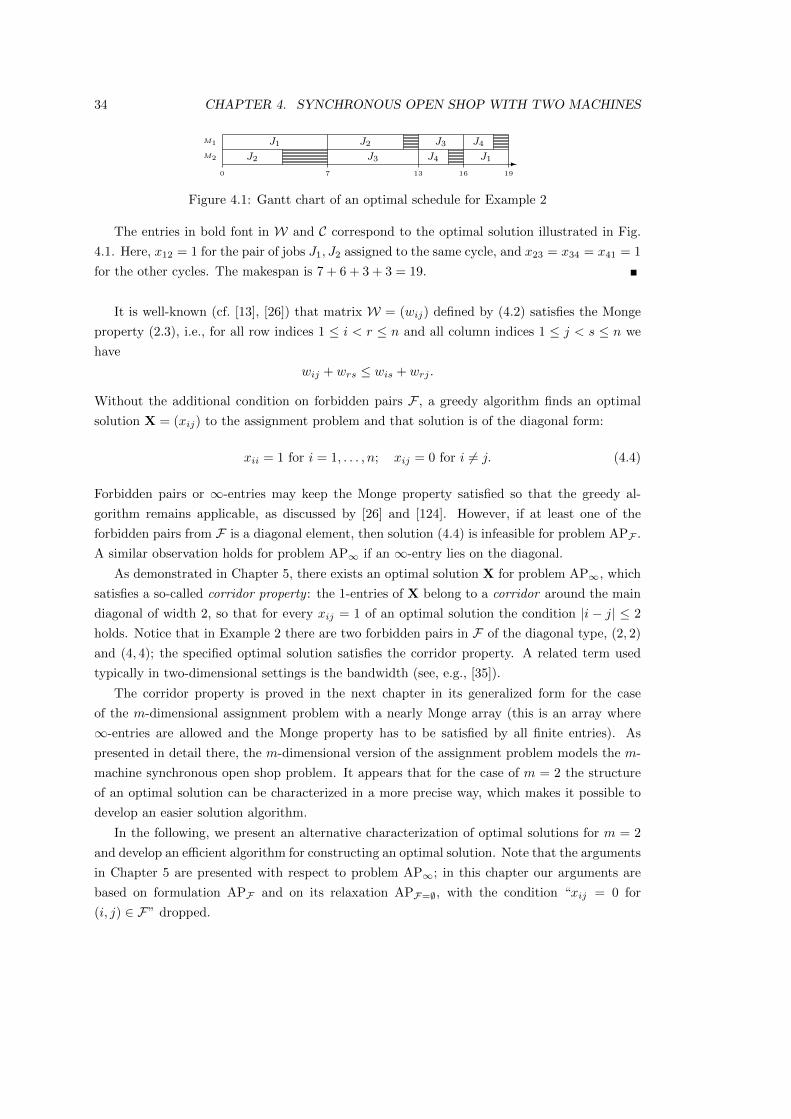
34 CHAPTER 4. SYNCHRONOUS OPEN SHOP WITH TWO MACHINES
-
J1
J2
J2
J3
J3
J4
J4
J1
M1
M2
0 7 13 16 19
Figure 4.1: Gantt chart of an optimal schedule for Example 2
The entries in bold font in W and C correspond to the optimal solution illustrated in Fig.
4.1. Here, x12 = 1 for the pair of jobs J1, J2 assigned to the same cycle, and x23 = x34 = x41 = 1
for the other cycles. The makespan is 7 + 6 + 3 + 3 = 19.
It is well-known (cf. [13], [26]) that matrix W = (wij) defined by (4.2) satisfies the Monge
property (2.3), i.e., for all row indices 1 ≤ i < r ≤ n and all column indices 1 ≤ j < s ≤ n we
have
wij + wrs ≤ wis + wrj .
Without the additional condition on forbidden pairs F , a greedy algorithm finds an optimal
solution X = (xij) to the assignment problem and that solution is of the diagonal form:
xii = 1 for i = 1, . . . , n; xij = 0 for i 6= j. (4.4)
Forbidden pairs or ∞-entries may keep the Monge property satisfied so that the greedy al-
gorithm remains applicable, as discussed by [26] and [124]. However, if at least one of the
forbidden pairs from F is a diagonal element, then solution (4.4) is infeasible for problem APF .
A similar observation holds for problem AP∞ if an ∞-entry lies on the diagonal.
As demonstrated in Chapter 5, there exists an optimal solution X for problem AP∞, which
satisfies a so-called corridor property : the 1-entries of X belong to a corridor around the main
diagonal of width 2, so that for every xij = 1 of an optimal solution the condition |i − j| ≤ 2
holds. Notice that in Example 2 there are two forbidden pairs in F of the diagonal type, (2, 2)
and (4, 4); the specified optimal solution satisfies the corridor property. A related term used
typically in two-dimensional settings is the bandwidth (see, e.g., [35]).
The corridor property is proved in the next chapter in its generalized form for the case
of the m-dimensional assignment problem with a nearly Monge array (this is an array where
∞-entries are allowed and the Monge property has to be satisfied by all finite entries). As
presented in detail there, the m-dimensional version of the assignment problem models the m-
machine synchronous open shop problem. It appears that for the case of m = 2 the structure
of an optimal solution can be characterized in a more precise way, which makes it possible to
develop an easier solution algorithm.
In the following, we present an alternative characterization of optimal solutions for m = 2
and develop an efficient algorithm for constructing an optimal solution. Note that the arguments
in Chapter 5 are presented with respect to problem AP∞; in this chapter our arguments are
based on formulation APF and on its relaxation APF=∅, with the condition “xij = 0 for
(i, j) ∈ F” dropped.

4.1. MINIMIZING THE MAKESPAN 35
A block Xh of size s is a square submatrix consisting of s × s elements with exactly one
1-entry in each row and each column of Xh. We call a block large if it is of size s ≥ 4, and small
otherwise. Our main result is establishing a block-diagonal structure of an optimal solution
X = (xij),
X =
X1 0 0 . . . 0
0 X2 0 . . . 0
. . .
0 . . . 0 Xz−1 0
0 . . . 0 0 Xz
(4.5)
with blocks Xh, 1 ≤ h ≤ z, of the form
(1),
(0 1
1 0
),
0 0 1
1 0 0
0 1 0
,
0 1 0
0 0 1
1 0 0
(4.6)
around the main diagonal, and 0-entries elsewhere. Note that the submatrix 0 0 1
0 1 0
1 0 0
is excluded from consideration.
Theorem 3. (“Small Block Property”): There exists an optimal solution to problem APF in
block-diagonal structure, containing only blocks of type (4.6).
The proof of the small block property
The general idea of the proof can be described as follows. Starting with an arbitrary optimal
solution which does not satisfy the small block property, replace repeatedly each block of size
s ≥ 4 by two blocks of cumulative size s, one of which is small. The replacement is performed
for the relaxed problem APF=∅, ignoring forbidden pairs F , but making sure that the cost of
the new solution (possibly infeasible in terms of F) is not larger than that of its predecessor.
Additionally, we keep 0-entries on the main diagonal unchanged, so that no new blocks of size
1 are created. As a result a new solution is constructed, feasible for APF=∅, of no higher cost
than the original one, consisting of small blocks only. If the constructed solution is infeasible
for APF , then at the next stage infeasible blocks of size 2 and 3 are replaced by feasible blocks,
also without increasing the cost, achieving an optimal solution consisting of small blocks.
First we prove the possibility of block splitting (Lemma 4), and then explain how infeasible
blocks can be converted into feasible ones (Lemmas 5 and 6 for blocks of size 2 and 3, respec-
tively). It leads to the main result (Theorem 3) – the existence of an optimal solution consisting

36 CHAPTER 4. SYNCHRONOUS OPEN SHOP WITH TWO MACHINES
of small blocks of type (4.6).
For a block consisting of 1-entries in rows and columns j1, j1 + 1, . . . , j1 + s− 1, renumber
those rows and columns as j1, j2, . . . , js with ji = j1 + i− 1, 1 ≤ i ≤ s. The cost associated
with block Xh is defined as
w (Xh) =
s∑u=1
s∑v=1
wjujvxjujv ,
so that the total cost of solution X with blocks (4.5) is
w (X) =
z∑h=1
w (Xh) .
Lemma 4. If an optimal solution to problem APF contains a block Xy of size s > 3, defined
over rows and columns j1, j2, . . . , js, then without increasing the cost it can be replaced by
two blocks, one block of size 2 or 3 defined over rows and columns j1, j2 or j1, j2, j3, and
one block defined over the remaining rows and columns. Furthermore, if a diagonal entry xjkjkin the initial solution is 0, then in the modified solution xjkjk is 0 as well.
Proof: Given a solution, we identify the non-zero entries in columns j1, j2 and j3, and denote
the corresponding rows by ja, jb, jc. For these indices we have
xjaj1 = 1, xjbj2 = 1, xjcj3 = 1. (4.7)
Furthermore, for non-zero entries in rows j1, j2, and j3, we denote the corresponding columns
by jt, ju, jv and have
xj1jt = 1, xj2ju = 1, xj3jv = 1. (4.8)
The proof is presented for the case
xj1j1 = xj2j2 = xj3j3 = 0. (4.9)
Notice that the case xj1,j1 = 1 contradicts the assumption that block Xy is large. In the case
of xj2j2 = 1 we replace block Xy by block X′y as shown in Fig. 4.2. Here the 1-entries which
are subject to change are enclosed in boxes and * denotes an arbitrary entry, 0 or 1. This
transformation involves 4 entries in rows j1, j2 and columns j2, jt. Notice that the marked
1-entries in the initial block Xy belong to a diagonal of type , while the marked 1-entries in
the resulting block X′y belong to a diagonal of type , so that w(X′y)≤ w (Xy) by the Monge
property.
In the case of xj1j1 = xj2j2 = 0, xj3j3 = 1, at least one of the values, a or t, is larger than
3 (a = 3 or t = 3 is not possible for xj3j3 = 1; a ≤ 2 and t ≤ 2 is not possible since block Xy
is large). If t > 3, then the transformation is similar to that in Fig. 4.2: it involves 4 entries in
rows j1, j3 and columns j3, jt. Alternatively, if a > 3, then the transformation involves 4
entries in rows j3, ja and columns j1, j3. In either case, the 1-entries in the initial solution

4.1. MINIMIZING THE MAKESPAN 37
Xy j1 j2 · · · jt · · · jsj1 0 0 · · · 1 · · · 0
j2 0 1 · · · 0 · · · 0j3 * 0 *...
......
. . ....
js * 0 · · · *
X′y j1 j2 · · · jt · · · js
j1 0 1 · · · 0 · · · 0
j2 0 0 · · · 1 · · · 0j3 * 0 *...
......
. . ....
js * 0 · · · *
Figure 4.2: Transformation of block Xy into X′y
belong to a diagonal of type and to a diagonal of type after the transformation, so that
the cost does not increase by the Monge property.
Thus, in the following we assume that condition (4.9) holds.
Case t = 2, or equivalently xj1j2 = 1. This implies b = 1. If a 6= u, then the transformation
from Xy to Xy shown in Fig. 4.3 creates a small block of size 2 without increasing the cost.
Xy j1jt,j2
· · · ju · · · jsjb, j1 0 1 · · · 0 · · · 0
j2 0 0 · · · 1 · · · 0...
......
......
ja 1 0 · · · 0 · · · 0...
......
......
js 0 0 · · · 0 · · · *
Xy j1jt,j2
· · · ju · · · jsjb, j1 0 1 · · · 0 · · · 0
j2 1 0 · · · 0 · · · 0...
......
......
ja 0 0 · · · 1 · · · 0...
......
......
js 0 0 · · · 0 · · · *
Figure 4.3: Transformation of block Xy into Xy
Consider the case a = u and notice that we can assume a = u > 3. Indeed, cases a = u = 1
and a = u = 2 cannot happen as the corresponding assignment is infeasible (see Fig. 4.4 (a)

38 CHAPTER 4. SYNCHRONOUS OPEN SHOP WITH TWO MACHINES
and (b)), and in case a = u = 3 the block is already small (see Fig. 4.4 (c)). For a = u > 3
the transformation illustrated in Fig. 4.3 is not applicable as it results in a new diagonal entry
xjaja = 1. Instead, we perform the two transformations from Xy to Xy and then to˜Xy shown
in Fig. 4.5 and 4.6, creating eventually a small block of size 3.
(a)
juj1
jtj2
ja, j1 1 1j2 1 0
(b)
j1jt,juj2
j1 0 1ja, j2 1 1
(c)
j1jtj2
juj3
j1 0 1 0j2 0 0 1ja, j3 1 0 0
Figure 4.4: Cases where t = 2 and a = u ≤ 3: (a) a = u = 1, (b) a = u = 2, (c) a = u = 3
Observe that both of the values, c and v, are different from a = u. Note further that we
have c 6= 1 as t = 2, c 6= 2 as u > 3, and c 6= 3 due to (4.9). Similarly v 6= 1 as a > 3, v 6= 2
as t = 2, and v 6= 3 due to (4.9). Thus c > 3 and v > 3. The relationship between a = u and
c is immaterial, as the above transformations work in both cases, a = u < c and a = u > c.
Similarly, the relationship between a = u and v is immaterial as well. Moreover, the presented
transformation works for either case, c = v or c 6= v.
Xy j1jt,j2
j3 · · · ja,ju
· · · jvjb, j1 0 1 0 · · · 0 · · · 0
j2 0 0 0 · · · 1 · · · 0j3 0 0 0 · · · 0 · · · 1
......
......
......
ju, ja 1 0 0 · · · 0 · · · 0...
......
......
...
jc 0 0 1 · · · 0 · · · 0
Xy j1jt,j2
j3 · · · ja,ju
· · · jvjb, j1 0 1 0 · · · 0 · · · 0
j2 0 0 1 · · · 0 · · · 0j3 0 0 0 · · · 0 · · · 1
......
......
......
ju, ja 1 0 0 · · · 0 · · · 0...
......
......
...
jc 0 0 0 · · · 1 · · · 0
Figure 4.5: Transformation from Xy to Xy
Case a = 2 is similar to the case of t = 2 since the X-matrices for these two cases are

4.1. MINIMIZING THE MAKESPAN 39
Xy j1jt,j2
j3 · · · ja,ju
· · · jvjb, j1 0 1 0 · · · 0 · · · 0j2 0 0 1 · · · 0 · · · 0
j3 0 0 0 · · · 0 · · · 1...
......
......
...
ju, ja 1 0 0 · · · 0 · · · 0...
......
......
...jc 0 0 0 · · · 1 · · · 0
˜Xy j1
jt,j2
j3 · · · ja,ju
· · · jvjb, j1 0 1 0 · · · 0 · · · 0j2 0 0 1 · · · 0 · · · 0
j3 1 0 0 · · · 0 · · · 0...
......
......
...
ju, ja 0 0 0 · · · 0 · · · 1...
......
......
...jc 0 0 0 · · · 1 · · · 0
Figure 4.6: Transformation from Xy to˜Xy
transposes of each other. Recall that whenever the swaps are done in the case of t = 2, the
1-entries on a diagonal of type become 0-entries, while the 0-entries on a diagonal of type
become 1-entries, so that the Monge inequality (2.3) is applicable. In the case of a = 2,
the initial 1-entries in the transpose matrix also belong to a diagonal of type , while the new
1-entries are created on a diagonal of type .
Case a > 2 and t > 2 with a < b and t < u. Consider the transformation from Xy to Xy
shown in Fig. 4.7. It uses the Monge property two times, once for the entries in rows j2, jaand columns j1, ju, and another time for the entries in rows j1, jb and columns j2, jt.
If a 6= u and b 6= t, then the resulting matrix Xy satisfies the conditions of the lemma and
a matrix without changed diagonal entries and with a small block of size 2 is obtained.
Consider the case a = u or b = t. By the definition of the indices a, b, t, u, according to
(4.7)-(4.8), we have a 6= b and t 6= u. The latter two conditions, combined with either a = u or
b = t, imply a 6= t and b 6= u.
Then, after Xy is transformed into Xy, we perform one more transformation from Xy toXy shown in Fig. 4.8. Then, the resulting matrix
Xy satisfies the conditions of the lemma.
Case a > 2 and t > 2 with a < b and t > u. We start with an additional pre-processing step
shown in Fig. 4.9 replacing x1t = x2u = 1 by 0-entries and x1u = x2t = 0 by 1-entries without
increasing the cost.
In the resulting matrix X∗y, we interchange the notation of the columns jt and ju in accor-
dance with definition (4.8) and proceed as described above for the case t < u. Since a > 2 and

40 CHAPTER 4. SYNCHRONOUS OPEN SHOP WITH TWO MACHINES
Xy j1 j2 · · · jt · · · juj1 0 0 · · · 1 · · · 0
j2 0 0 · · · 0 · · · 1...
......
......
ja 1 0 · · · 0 · · · 0...
......
......
jb 0 1 · · · 0 · · · 0
Xy j1 j2 · · · jt · · · juj1 0 1 · · · 0 · · · 0
j2 1 0 · · · 0 · · · 0...
......
......
ja 0 0 · · · 0 · · · 1...
......
......
jb 0 0 · · · 1 · · · 0
Figure 4.7: Transformation from Xy to Xy
Xy j1 j2 · · · jt · · · juj1 0 1 · · · 0 · · · 0j2 1 0 · · · 0 · · · 0
......
......
...
ja 0 0 · · · 0 · · · 1...
......
......
jb 0 0 · · · 1 · · · 0
Xy j1 j2 · · · jt · · · juj1 0 1 · · · 0 · · · 0j2 1 0 · · · 0 · · · 0
......
......
...
ja 0 0 · · · 1 · · · 0...
......
......
jb 0 0 · · · 0 · · · 1
Figure 4.8: Transformation from Xy toXy
therefore u 6= 1, no new diagonal entry is produced in the pre-processing.
Case a > 2 and t > 2 with a > b. This case corresponds to the transposed of the picture in
the previous case. We undertake a similar pre-processing step as before, to transform this case
into one with a < b.

4.1. MINIMIZING THE MAKESPAN 41
Xy j1 j2 · · · ju · · · jtj1 0 0 · · · 0 · · · 1
j2 0 0 · · · 1 · · · 0...
......
......
ja 1 0 · · · 0 · · · 0...
......
......
jb 0 1 · · · 0 · · · 0
X∗y j1 j2 · · · ju · · · jt
j1 0 0 · · · 1 · · · 0
j2 0 0 · · · 0 · · · 1...
......
......
ja 1 0 · · · 0 · · · 0...
......
......
jb 0 1 · · · 0 · · · 0
Figure 4.9: Transformation from Xy to X∗y
Lemma 5. If a solution X contains an infeasible block of size 2, i.e., xj1,j2 = xj2,j1 = 1 with
at least one of the entries (j1, j2) or (j2, j1) belonging to F , then without increasing the cost it
can be replaced by two feasible blocks of size 1, given by xj1,j1 = 1 and xj2,j2 = 1.
Proof: For the above transformation the cost does not increase due to the Monge property. As
far as feasibility is concerned, by the definition of set F , there is exactly one forbidden entry in
each row and each column. Thus, if (j1, j2) ∈ F , then neither (j1, j1) nor (j2, j2) are forbidden.
Similar arguments hold for (j2, j1) ∈ F .
Lemma 6. If a solution X contains an infeasible block of size 3, then that block can be replaced,
without increasing the cost, by three feasible blocks of size 1, or by two feasible blocks, one of
size 1 and another one of size 2.
Proof: Let Xy be an infeasible block consisting of rows and columns j1, j2 and j3. The proof
is presented for the case
xj1j1 = xj3j3 = 0;
otherwise Xy can be decomposed into smaller blocks. Under the above assumption, Xy is of
one of the three types X(I)y , X
(II)y or X
(III)y , shown in Fig. 4.10.
Notice that X(III)y can be replaced by X
(II)y without increasing the cost, using the Monge
property, and so we only have to deal with X(I)y and X
(II)y , which are symmetric. We first
demonstrate that each block, X(I)y or X
(II)y , can be replaced by blocks X
(a)y , X
(b)y or X
(c)y shown
in Fig. 4.11, without increasing the cost. Then we proof that at least one of those blocks is
feasible.

42 CHAPTER 4. SYNCHRONOUS OPEN SHOP WITH TWO MACHINES
X(I)y j1 j2 j3
j1 0 0 1j2 1 0 0j3 0 1 0
X(II)y j1 j2 j3
j1 0 1 0j2 0 0 1j3 1 0 0
X(III)y j1 j2 j3
j1 0 0 1j2 0 1 0j3 1 0 0
Figure 4.10: Blocks X(I)y , X
(II)y and X
(III)y
X(a)y j1 j2 j3
j1 1 0 0j2 0 0 1j3 0 1 0
X(b)y j1 j2 j3
j1 0 1 0j2 1 0 0j3 0 0 1
X(c)y j1 j2 j3
j1 1 0 0j2 0 1 0j3 0 0 1
Figure 4.11: Blocks X(a)y , X
(b)y and X
(c)y
The transformation of X(I)y into X
(a)y or X
(b)y involves a quadruple of 1-entries, so that
the cost does not increase due to the Monge property. Transforming X(I)y into the diagonal
solution X(c)y we achieve a minimum cost assignment for the Monge submatrix given by rows
and columns j1, j2, j3 (see, e.g., [26]). The same arguments hold for the transformation of
X(II)y into X
(a)y , X
(b)y or X
(c)y .
In the following, we deal with feasibility. If the initial infeasible block is of type X(I)y , then
at least one of the pairs (j1, j3), (j2, j1) or (j3, j2) is forbidden. Therefore, at least one pair
(j1, j1) or (j3, j3) is feasible. If (j1, j1) is feasible, then block X(a)y or X
(c)y is feasible. Similarly,
if (j3, j3) is feasible, then block X(b)y or X
(c)y is feasible.
Similar arguments can be used if the initial infeasible block is of type X(II)y .
Combining Lemmas 4-6 and using them repeatedly we arrive at the main result of Theorem 3.
Below we present the formal proof.
Proof of Theorem 3: Consider any optimal solution. Apply Lemma 4 repeatedly until
all blocks are of size 1, 2, or 3. Since all diagonal 1-entries of the new solution are also present
in the original solution, those entries are feasible. Therefore, all blocks of size 1 are feasible.
By Lemmas 5-6 all blocks of size 2 or 3 are either feasible or can be converted into feasible
blocks without increasing the cost. Thus, the resulting solution has blocks of size 1, 2 and 3, it
is feasible, and its cost is not larger than the cost of the original optimal solution.
Finally, the only small blocks that are not of type (4.6), have three 1’s on the secondary
diagonal, since other configurations of 0’s and 1’s combine blocks of type (4.6). Due to the

4.1. MINIMIZING THE MAKESPAN 43
arguments used in the proof of Lemma 6 with respect to block X(III)y , such blocks can also be
eliminated, which concludes the proof.
A linear time dynamic programming algorithm to solve problem APF
The small block property leads to an efficient O(n)-time dynamic programming algorithm to
find an optimal solution. Here we use formulation AP∞ rather than APF , as infinite costs can
be easily handled by recursive formulae. The algorithm enumerates optimal partial solutions,
extending them repeatedly by adding blocks of size 1, 2 or 3.
Let Si denote an optimal partial solution for a subproblem of AP∞ defined by the submatrix
of W with the first i rows and i columns. If an optimal partial solution Si is known, together
with solutions Si−1 and Si−2 for smaller subproblems, then by Theorem 3 the next optimal
partial solution Si+1 can be found by selecting one of the following three options:
- extending Si by adding a block of size 1 with xi+1,i+1 = 1; the cost of the assignment increases
by wi+1,i+1;
- extending Si−1 by adding a block of size 2 with xi,i+1 = xi+1,i = 1; the cost of the assignment
increases by wi,i+1 + wi+1,i;
- extending Si−2 by adding a block of size 3 with the smallest cost:
(i) xi−1,i+1 = xi,i−1 = xi+1,i = 1 with the cost wi−1,i+1 + wi,i−1 + wi+1,i, or
(ii) xi−1,i = xi,i+1 = xi+1,i−1 with the cost wi−1,i + wi,i+1 + wi+1,i−1.
Let w(Si) denote the cost of Si. Then
w(Si+1) = min w(Si) + wi+1,i+1,
w(Si−1) + wi,i+1 + wi+1,i,
w(Si−2) + wi−1,i + wi,i+1 + wi+1,i−1,
w(Si−2) + wi−1,i+1 + wi,i−1 + wi+1,i .
(4.10)
The initial conditions are defined as follows:
w(S0) = 0,
w(S1) = w11,
w(S2) = min w11 + w22, w12 + w21 .
Thus, w(S3), . . . , w(Sn) are computed by (4.10) in O(n) time.
Theorem 7. Problem O2|synmv|Cmax is solvable in O(n) time, after pre-sorting.

44 CHAPTER 4. SYNCHRONOUS OPEN SHOP WITH TWO MACHINES
Further implications of the small block property
Concluding this subsection, we provide several observations about the presented results. First,
the small block property for problem O2|synmv|Cmax has implications for the assignment prob-
lem AP∞ with costs (4.3) and for more general cost matrices. The proof of the small block
property is presented for problem APF . It is easy to verify that the proof is valid for an arbi-
trary Monge matrix W, not necessarily of type (4.2); the important property used in the proof
requires that the set F has no more than one forbidden pair (i, j) in every row and in every col-
umn, and that all entries of the matrixW, including those corresponding to the forbidden pairs
F , satisfy the Monge property. Thus, the small block property and the O(n)-time algorithm
hold for problem AP∞ if
(i) there is no more than one∞-entry in every row and every column of the cost matrix C, and
(ii) matrix C can be transformed into a Monge matrix by modifying only the∞-entries, keeping
other entries unchanged.
Note that not every nearly Monge matrix satisfying (i) can be completed into a Monge
matrix satisfying (ii); see Section 5.4 in the next chapter for further details. However, the
definition (4.3) of the cost matrix C for the synchronous open shop allows a straightforward
completion by replacing every entry cij = ∞ by cij = max ai, bj. While completability is
not used in the proof of the more general corridor property presented in Chapter 5, the proof
of the small block property depends heavily on the fact that the matrix of the synchronous
open shop problem can be completed into a Monge matrix. In particular, we use completability
when we accept potentially infeasible blocks in the proof of Lemma 4 and repair them later on
with the help of Lemmas 5 and 6. In the literature, the possibility of completing an incomplete
Monge matrix (a matrix with unspecified entries) was explored by [41] for the traveling salesman
problem. They discuss Supnick matrices, a subclass of incomplete Monge matrices, for which
completability is linked with several nice structural and algorithmic properties.
Finally, we observe that while the assignment matrices arising from the multi-machine case
are completable in the same way as for the two-machine case (see again the next chapter), it
remains open whether this can be used to obtain an improved result for more than two machines
as well. The technical difficulties of that case are beyond the scope of this thesis.
4.1.2 Problem O2|synmv, rel|Cmax
In this section, we consider the relaxed problem O2|synmv, rel|Cmax where more than n cycles
are allowed, with unallocated (idle) machines in some cycles. Recall that we model idle intervals
on machines by introducing dummy jobs with zero-length operations on both machines (aj =
bj = 0 for a dummy job Jj). Given a set of n actual jobs, denote an optimal makespan for
problem O2|synmv|Cmax without dummy jobs by C∗max, while the optimal makespan for the
relaxed problem O2|synmv, rel|Cmax with dummy jobs is denoted by Crmax. An example shown

4.1. MINIMIZING THE MAKESPAN 45
in Fig. 4.12 illustrates that the introduction of dummy jobs can reduce the makespan. In that
example, the input data is as follows:
j 1 2 3 4
aj 5 5 5 1
bj 5 5 5 1
Figure 4.12: Two open shop schedules, Crmax < C∗max: (a) An optimal schedule with one dummyjob paired with job 1; (b) An optimal schedule without dummy jobs.
Any feasible schedule for problem O2|synmv|Cmax is also feasible for O2|synmv, rel|Cmax,
which implies that Crmax ≤ C∗max. If in the optimal schedule Sr for problem O2|synmv, rel|Cmax
schedule no dummy jobs are used, then Crmax = C∗max. Below we investigate properties of
instances for which Crmax < C∗max.
Note that whenever in a schedule S for problem O2|synmv, rel|Cmax a cycle appears con-
sisting only of dummy operations, we can remove that cycle from the schedule and renumber all
dummy operations and dummy jobs in order to end up with a schedule of the same makespan,
which uses one less dummy job. Thus we can assume that in any schedule S for problem
O2|synmv, rel|Cmax there is no cycle consisting only of dummy operations.
We first show that at most one dummy job is needed in order obtain an optimal schedule
for problem O2|synmv, rel|Cmax.
Lemma 8. There exists an optimal schedule for problem O2|synmv, dummy|Cmax with at most
one dummy job used, so that the number of cycles is no more than n+ 1.
Proof: Suppose in an optimal schedule Sr there are two dummy jobs Ju and Jv, in addition
to (possibly) other dummy jobs. Let the four cycles in which those dummy jobs appear be

46 CHAPTER 4. SYNCHRONOUS OPEN SHOP WITH TWO MACHINES
∣∣JuJj1
∣∣, ∣∣Jj2Ju
∣∣, ∣∣ JvJj3∣∣ and∣∣Jj4Jv
∣∣, where Jj1 , Jj2 , Jj3 and Jj4 are the real jobs, not necessarily pairwise
different.
If Jj1 6= Jj2 , then combining the first two cycles∣∣JuJj1
∣∣, ∣∣Jj2Ju
∣∣ into∣∣Jj2Jj1
∣∣ and eliminating the
dummy job Ju results in a schedule S′ with the makespan C ′max such that
C ′max − Crmax = maxaj2 , bj1 − (aj2 + bj1) ≤ 0.
Since Sr is optimal, so is S′.
If Jj1 = Jj2 , but Jj3 6= Jj4 , then a similar transformation is applied to∣∣ JvJj3
∣∣, ∣∣Jj4Jv
∣∣ resulting
in∣∣Jj4Jj3
∣∣.Consider now the case that Jj1 = Jj2 and Jj3 = Jj4 , i.e., the four cycles are of the form∣∣Ju
Jj1
∣∣, ∣∣Jj1Ju
∣∣, ∣∣ JvJj3∣∣, ∣∣Jj3Jv ∣∣. We combine these four cycles into two cycles∣∣Jj1Jj3
∣∣, ∣∣Jj3Jj1
∣∣, eliminating the
dummy jobs Ju and Jv. Denoting the resulting schedule by S′′ and its makespan by C ′′max we
conclude:
C ′′max − Crmax = (maxaj1 , bj3+ maxaj3 , bj1)− (aj1 + bj1 + aj3 + bj3) ≤ 0.
Again, S′′ is optimal due to the optimality of Sr.
This way, in any optimal schedule with at least two dummy jobs, we can reduce the number
of dummy jobs by at least one without increasing the makespan. Consequently, an optimal
schedule with at most one dummy job must exist.
Note that this means that problem O2|synmv, rel|Cmax can be solved in linear time (after
sorting the processing times in the order given by (4.1)). Indeed, given an instance of problem
O2|synmv, rel|Cmax with n jobs, we first add dummy job Jn+1 with processing times an+1 =
bn+1 = 0 in order to use the results from the last section. Then, similar to the problem without
dummy jobs, we solve assignment problem APF with the extended (n + 1) × (n + 1) weight
matrix given by
wij = max ai, bj , 1 ≤ i, j ≤ n+ 1.
and set of forbidden entries F = (1, j1), (2, j2), . . . , (n, jn), where operations O1,i and O2,ji
belong to the same job. Note that compared to the last section, the weight matrix is extended
by one line and one column, but the set of forbidden entries remains the same as without the
dummy job (we allow for the two operations of a dummy job to be placed in the same cycle, in
which case the dummy job is not needed to achieve an optimal schedule).
Later, in Chapter 6, we will see that the result of Lemma 8 is generalizable, in the sense
that for problem O|synmv, rel|Cmax with m machines an optimal schedule exists in which at
most m − 1 dummy jobs are used, so that the number of cycles is at most n + m − 1 and we
show that the bound is tight for any number m of machines. Observe that in the case of two
machines the example in Figure 4.12 suffices to show tightness.
For two machines, we can additionally provide strong necessary conditions for instances in
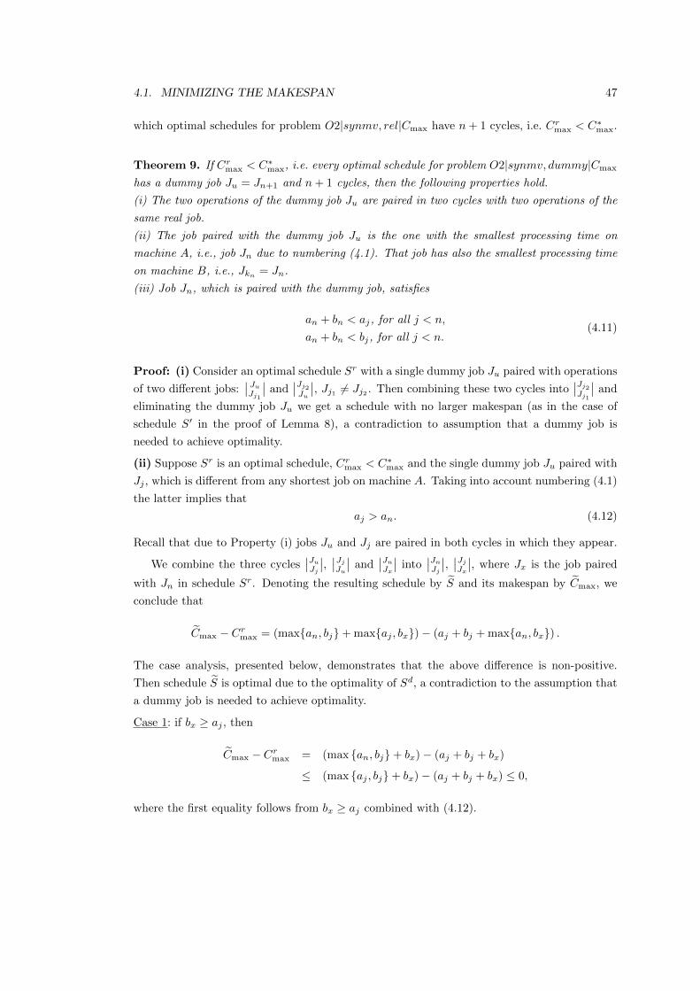
4.1. MINIMIZING THE MAKESPAN 47
which optimal schedules for problem O2|synmv, rel|Cmax have n+ 1 cycles, i.e. Crmax < C∗max.
Theorem 9. If Crmax < C∗max, i.e. every optimal schedule for problem O2|synmv, dummy|Cmax
has a dummy job Ju = Jn+1 and n+ 1 cycles, then the following properties hold.
(i) The two operations of the dummy job Ju are paired in two cycles with two operations of the
same real job.
(ii) The job paired with the dummy job Ju is the one with the smallest processing time on
machine A, i.e., job Jn due to numbering (4.1). That job has also the smallest processing time
on machine B, i.e., Jkn = Jn.
(iii) Job Jn, which is paired with the dummy job, satisfies
an + bn < aj, for all j < n,
an + bn < bj, for all j < n.(4.11)
Proof: (i) Consider an optimal schedule Sr with a single dummy job Ju paired with operations
of two different jobs:∣∣JuJj1
∣∣ and∣∣Jj2Ju
∣∣, Jj1 6= Jj2 . Then combining these two cycles into∣∣Jj2Jj1
∣∣ and
eliminating the dummy job Ju we get a schedule with no larger makespan (as in the case of
schedule S′ in the proof of Lemma 8), a contradiction to assumption that a dummy job is
needed to achieve optimality.
(ii) Suppose Sr is an optimal schedule, Crmax < C∗max and the single dummy job Ju paired with
Jj , which is different from any shortest job on machine A. Taking into account numbering (4.1)
the latter implies that
aj > an. (4.12)
Recall that due to Property (i) jobs Ju and Jj are paired in both cycles in which they appear.
We combine the three cycles∣∣JuJj
∣∣, ∣∣JjJu∣∣ and∣∣JnJx
∣∣ into∣∣JnJj
∣∣, ∣∣JjJx∣∣, where Jx is the job paired
with Jn in schedule Sr. Denoting the resulting schedule by S and its makespan by Cmax, we
conclude that
Cmax − Crmax = (maxan, bj+ maxaj , bx)− (aj + bj + maxan, bx) .
The case analysis, presented below, demonstrates that the above difference is non-positive.
Then schedule S is optimal due to the optimality of Sd, a contradiction to the assumption that
a dummy job is needed to achieve optimality.
Case 1: if bx ≥ aj , then
Cmax − Crmax = (max an, bj+ bx)− (aj + bj + bx)
≤ (max aj , bj+ bx)− (aj + bj + bx) ≤ 0,
where the first equality follows from bx ≥ aj combined with (4.12).

48 CHAPTER 4. SYNCHRONOUS OPEN SHOP WITH TWO MACHINES
Case 2: if bx < aj and in addition bx ≤ an, then
Cmax − Crmax = (max an, bj+ aj)− (aj + bj + an) ≤ 0.
Case 3: if bx < aj and bx > an, then
Cmax − Crmax = (max an, bj+ aj)− (aj + bj + bx)
≤ (max bx, bj+ aj)− (aj + bj + bx) ≤ 0.
The second part of Property (ii), stating that the job paired with the dummy job has the
smallest processing time on machine B can be proved similarly.
(iii) Let Sr be an optimal schedule and suppose in Sr dummy job Ju is paired with Jn which
is a shortest job on machine A and in accordance with Property (ii) also on machine B,
bn ≤ bj for any j = 1, 2, . . . , n.
Suppose further there exists a job Jh that does not satisfy (4.11). Without loss of generality
we assume
an + bn ≥ ah. (4.13)
Similar to the proof of property (ii), we combine the three cycles∣∣JuJn
∣∣, ∣∣JnJu∣∣ and∣∣JhJx
∣∣ into∣∣JnJx
∣∣and
∣∣JhJn
∣∣, where Jx is now the job paired with Jh in schedule Sr. For the resulting schedule S
and for the initial schedule Sr, the change in the makespan is given by
Cmax − Crmax = (maxan, bx+ maxah, bn)− (an + bn + maxah, bx) .
Using conditions
maxan, bx ≤ maxah, bx,maxah, bn ≤ an + bn,
where the first one follows from an ≤ ah, while the second one follows from (4.13), we conclude
that
Cmax − Crmax ≤ (maxah, bx+ maxah, bn)− (an + bn + maxah, bx) ≤ 0.
As before, the resulting optimality of schedule S is in contradiction to the assumption that a
dummy job is needed to achieve optimality.
Notice that conditions (4.11) are necessary but not sufficient for Crmax < C∗max. For example,
for the instance given by the table below conditions (4.11) are satisfied, but an optimal schedule
without dummy jobs has a smaller makespan than an optimal schedule with a dummy job, see
Fig. 4.13 (a)-(b).

4.2. SCHEDULING WITH DEADLINES 49
j 1 2 3 4
aj 5 5 3 1
bj 5 5 3 1
Figure 4.13: An example illustrating that conditions (4.11) are not sufficient for introducinga dummy job: (a) an optimal schedule with one dummy job; (b) an optimal schedule withoutdummy jobs.
4.2 Scheduling with deadlines
In this section, we consider problem O|synmv,Cj ≤ Dj |−, where each job Jj , 1 ≤ j ≤ n, has a
given deadline Dj by which it has to be completed. We prove that finding a feasible schedule
with all jobs meeting their deadlines is NP-complete in the strong sense even if there are only
two machines and each job has only one non-zero processing time. Furthermore, we show that
problem O2|synmv,Cj ≤ Dj , Dj ∈ D′, D′′|−, where the set of all deadlines is limited to two
values, is at least NP-complete in the ordinary sense. The proofs presented below are based on
the ideas of [18] who established the complexity status of the parallel batching problem with
deadlines.
Consider the 3-PARTITION problem (3-PART) known to be strongly NP-complete, cf. [59].
Given a set Q = 1, . . . , 3q, q ∈ N, a bound E ∈ N and natural numbers ei for every i ∈ Q,
satisfying∑i∈Q ei = qE and E
4 < ei <E2 , can Q be partitioned into q subsets Qk, 1 ≤ k ≤ q,
such that∑i∈Qk ei = E for all k?
Based on an instance of 3-PART, we construct an instance I(q) of the two-machine syn-
chronous open shop problem O2|synmv,Cj ≤ Dj |− with n = 6q2 jobs, q deadlines and two
machines, denoted by A and B. Each job Jj,l has two indices j and l to distinguish between

50 CHAPTER 4. SYNCHRONOUS OPEN SHOP WITH TWO MACHINES
jobs of different types, j = 1, 2, . . . , 2q and l = 1, 2, . . . , 3q. We introduce constants
T =
3q∑i=1
i, Tj =
j∑i=1
i, W = q3E.
For each l, 1 ≤ l ≤ 3q, the processing times aj,l and bj,l of the jobs Jj,l on machines A and B
are defined as follows:
aj,l = lW + (q − j)el, bj,l = 0 for 1 ≤ j ≤ q;aq+1,l = 0, bq+1,l = lW + qel;
aj,l = 0, bj,l = lW for q + 2 ≤ j ≤ 2q.
The deadlines Dj,l are set to
Dj,l = jTW + (jq2 − Tjq + Tj)E for 1 ≤ j ≤ q;Dj,l = qTW + (q3 − Tqq + Tq)E for q + 1 ≤ j ≤ 2q.
Throughout the proof we use the following terms for different classes of jobs. Parameter
l, 1 ≤ l ≤ 3q, characterizes jobs of type l. For each value of l there are 2q jobs of type l,
q of which have non-zero A-operations (we call these A-jobs) and the remaining q jobs have
non-zero B-operations (we call these B-jobs). Among the q B-jobs of type l, there is one long
B-job of type l, namely Jq+1,l with processing time lW + qel, and there are q − 1 short B-jobs
of type l, namely Jq+2,l, Jq+3,l, . . . , J2q,l, each with processing time lW . Overall, there are 3q
long B-jobs, one of each type l, 1 ≤ l ≤ 3q, and 3q (q − 1) short B-jobs, with q − 1 short jobs
of each type l. Note that, independent of l, job Jj,l is an A-job if 1 ≤ j ≤ q, and a B-job if
q + 1 ≤ j ≤ 2q.
With respect to the deadlines, the jobs with non-zero B-operations are indistinguishable.
The jobs with non-zero A-operations have deadlines Dj,l depending on j; we refer to those jobs
as componentj A-jobs. For each j, there are 3q jobs of that type.
Lemma 10. If there exists a solution Q1, Q2, . . . , Qq to an instance of 3-PART, then there exists
a feasible schedule for the instance I(q) of the two-machine synchronous open shop problem with
q deadlines.
Proof: We construct a schedule S∗ consisting of q components Γ1,Γ2, . . . ,Γq, each of which
consists of 3q cycles, not counting zero-length cycles. In component Γk, 1 ≤ k ≤ q, machine A
processes 3q componentk A-jobs, one job of each type l, l = 1, 2, . . . , 3q. Machine B processes
3 long B-jobs and 3 (q − 1) short B-jobs, also one job of each type l, l = 1, 2, . . . , 3q.
Within one component, every cycle combines an A-job and a B-job of the same type l,
1 ≤ l ≤ 3q. The ordering of cycles in each component is immaterial, but component Γk
precedes component Γk+1, 1 ≤ k ≤ q − 1. If Qk = l1, l2, l3 is one of the sets of the solution
to 3-PART, then the three long B-jobs Jq+1,l1 , Jq+1,l2 , Jq+1,l3 are assigned to cycle Γk.

4.2. SCHEDULING WITH DEADLINES 51
Finally, there are 3q2 cycles of length zero. We assume that each zero-length operation is
scheduled immediately after the non-zero operation of the same job. The resulting schedule S∗
is shown in Fig. 4.14.
(lW + (q−1)el
lW+qel
)l∈Q1
(lW + (q−1)el
lW
)l∈Q\Q1
component 1
(lW + (q−2)el
lW+qel
)l∈Q2
(lW + (q−2)el
lW
)l∈Q\Q2
component 2
...
(lW + (q−k)el
lW+qel
)l∈Qk
(lW + (q−k)el
lW
)l∈Q\Qk
component k
...
(lW
lW+qel
)l∈Qq
(lWlW
)l∈Q\Qq
component q
Figure 4.14: Schedule derived from a solution to 3-PART
It is easy to verify that if Q1, Q2, . . . , Qq define a solution to the instance of 3-PART, then
the constructed schedule S∗ is feasible with all jobs meeting their deadlines.
We now prove the reverse statement. The proof is structured into a series of properties
where the last one is the main result of the lemma.
Lemma 11. If there exists a feasible schedule S for the instance I(q) of the synchronous open
shop problem with q deadlines, then the following properties hold:
(1) each cycle of non-zero length contains an A-job of type l and a B-job of the same type l,
l = 1, 2, . . . , 3q; without loss of generality we can assume that each zero length operation
is scheduled in the cycle immediately after the non-zero length operation of the same job;
(2) no componentj A-job is scheduled on machine A before any componenti A-job, with 1 ≤i ≤ j − 1; hence S is splittable into components Γ1,Γ2, . . . ,Γq in accordance with A-jobs;
(3) each component Γj, 1 ≤ j ≤ q, defines a set Qj of indices that correspond to long B-
jobs scheduled in Γj; the resulting sets Q1, Q2, . . . , Qq define a solution to the instance of
3-PART.
Proof: (1): In a feasible schedule S satisfying the first property, all cycles have a balanced
workload on machines A and B: in any component Γk, 1 ≤ k ≤ q, the cycle lengths are W ,
2W , . . . , 3qW , with the value qel or (q− k)el added. Thus, the total length of such a schedule
is at least q · TW . For a schedule that does not satisfy the first property, the machine load is
not balanced in at least two cycles, so that the lW -part of the processing time does not coincide
in these cycles. Thus, the total length of such a schedule is at least qTW +W = qTW + q3E.
Since q > 1, the latter value exceeds the largest possible deadline
max1≤j≤2q,1≤l≤3q
Dj,l = qTW + (q3 − Tqq + Tq)E,
a contradiction.

52 CHAPTER 4. SYNCHRONOUS OPEN SHOP WITH TWO MACHINES
Note that the above especially shows that zero length operations are only paired in cycles
with other zero length operations. Therefore, we can assume without loss of generality that
zero length operations are scheduled immediately after the non-zero length operations of the
same job. Indeed, if this is not the case, we can change the order of cycles, and possibly the
assignment of zero length operations to the zero length cycles in order to achieve the assumed
structure, without changing the feasibility of the schedule.
(2): Consider a schedule S in which all componentu A-jobs precede componentu+1 A-jobs
for u = 1, 2, . . . , i − 1, but after that a sequence of componenti A-jobs is interrupted by at
least one componentj A-job with j > i. Let the very last componenti A-job scheduled in S
be Ji,v for some 1 ≤ v ≤ 3q. Then the completion time of the cycle associated with Ji,v is at
least iTW + W , where TW is a lower bound on the total length of all componentu A-jobs,
u = 1, 2, . . . , i, and W is the smallest length of a cycle that contains the violating componentj
A-job. Since W is large, job Ji,v does not meet its deadline
Di,v = iTW + (iq2 − Tiq + Ti)E,
a contradiction.
The second property implies that on machine A all component1 A-jobs are scheduled first,
followed by all component2 A-jobs, etc. Thus, the sequence of jobs on machine A defines a
splitting of the schedule S into components Γ1,Γ2, . . . ,Γq.
(3): Given a schedule S satisfying the first two properties, we first define sets Q1, Q2, . . . , Qq
and then show that they provide a solution to 3-PART.
Schedule S consists of components Γj , 1 ≤ j ≤ q. In each component Γj machine A processes
all componentj A-jobs Jj,l (1 ≤ l ≤ 3q), each of which is paired with a B-job of the same type
l. Recall that a B-job Jq+1,l of type l is long, with processing time lW + qel. All other B-jobs
Jj,l, q + 2 ≤ j ≤ 2q, of type l are short, with processing time lW . Considering the long B-jobs
of component Γj , define a set Qj of the associated indices, i.e., l ∈ Qj if and only if the long
B-job Jq+1,l is scheduled in component Γj . Denote the sum of the associated numbers in Qj
by e(Qj) :=∑l∈Qj el.
The length of any cycle in component Γj is either aj,l = lW + (q − j)el if the componentj
A-job of type l is paired with a short B-job of type l, or bq+1,l = lW + qel if it is paired with
the long B-job Jq+1,l. Then the completion time CΓj of component Γj , 1 ≤ j ≤ q, can be
calculated as
CΓj =
j∑h=1
∑l∈Qh
[lW + qel] +∑
l∈Q\Qh[lW + (q − h)el]
=
j∑h=1
(TW + (q − h)qE + he(Qh)),
which for a feasible schedule S does not exceed the common deadlineDj,l of A-jobs in component

4.2. SCHEDULING WITH DEADLINES 53
Γj , Dj,l = jTW + jq2E − TjqE + TjE =∑jh=1 (TW + (q − h)qE + hE) . Notice that the
deadline of any B-job in component Γj is not less than Dj,l. Thus, for any j, 1 ≤ j ≤ q we get
Dj,l − CΓj =
j∑h=1
(TW + (q − h)qE + hE)
−j∑
h=1
(TW + (q − h)qE + he(Qh))
=
j∑h=1
h (E − e(Qh)) ≥ 0. (4.14)
If all inequalities in (4.14) hold as equalities, i.e.,
j∑h=1
h (E − e(Qh)) = 0, j = 1, 2, . . . , q,
then it is easy to prove by induction that E− e(Qh) = 0 for each h = 1, . . . , q and therefore the
partition Q1, Q2, . . . , Qq of Q defines a solution to 3-PART.
Assume the contrary, i.e., there is at least one strict inequality in (4.14). Then a linear
combination L of inequalities (4.14) with strictly positive coefficients has to be strictly positive.
Using coefficients 1j − 1
j+1 for j = 1, 2, . . . , q − 1 and 1q for j = q we obtain:
L =
q−1∑j=1
[(1
j− 1
j + 1
) j∑h=1
h (E − e(Qh))
]+
1
q
q∑h=1
h (E − e(Qh)) > 0.
It follows that
0 < L =
q−1∑h=1
h (E − e(Qh))
q−1∑j=h
(1
j− 1
j + 1
)+1
q
q∑h=1
h (E − e(Qh))
=
q−1∑h=1
[h (E − e(Qh))
(1
h− 1
q
)]+
1
q
q∑h=1
h (E − e(Qh))
=
q∑h=1
(E − e(Qh)) = 0,
where the last equality follows from the definition of E for an instance of 3-PART. The obtained
contradiction proves the third property of the lemma.
Lemmas 10 and 11 together imply the following result.
Theorem 12. Problem O2|synmv,Cj ≤ Dj |− is NP-complete in the strong sense, even if each
job has only one non-zero operation.

54 CHAPTER 4. SYNCHRONOUS OPEN SHOP WITH TWO MACHINES
Similar arguments can be used to formulate a reduction from the PARTITION problem
(PART) to the two-machine synchronous open shop problem, instead of the reduction from 3-
PART. Notice that in the presented reduction from 3-PART all B-jobs have the same deadline,
while A-jobs have q different deadlines, one for each component Γj defining a set Qj . In the
reduction from PART we only require two different deadlines D,D′, one for each of the two
sets corresponding to the solution to PART. Similar to the reduction from 3-PART, we define
component1 A-jobs with deadline D and component2 A-jobs with deadline D′ which define
a splitting of the schedule into two components Γ1,Γ2. For each of the natural numbers of
PART we define one long B-job and one short B-job and show that the distribution of the long
jobs within the two components of the open shop schedule corresponds to a solution of PART.
Omitting the details of the reduction, we state the following result.
Theorem 13. Problem O2|synmv,Cj ≤ Dj , Dj ∈ D′, D′′|− with only two different deadlines
is at least ordinary NP-complete, even if each job has only one non-zero operation.
At the end of this section we note that the complexity of the relaxed versions of the prob-
lems, which allow incomplete cycles modelled via dummy jobs, remains the same as stated in
Theorems 12 and 13. Indeed, Property 1 of Lemma 11 stating that each non-zero operation
of some job is paired with a non-zero operation of another job, still holds for the version with
dummy jobs. Therefore, in the presence of dummy jobs a schedule meeting the deadlines has
the same component structure as in Lemmas 10 and 11, so that the same reduction from 3-
PART (PART) works for proving that O2|synmv, rel, Cj ≤ Dj |− is strongly NP-complete and
O2|synmv, rel, Cj ≤ Dj , Dj ∈ D′, D′′ |− is at least ordinary NP-complete.
4.3 Minimizing the total completion time
In this section, we prove that the synchronous open shop problem with the total completion
time objective is strongly NP-hard even in the case of m = 2 machines. The proof uses some
ideas from [128] in which the NP-hardness of problem F2|no−wait|∑Cj is proved. Note that
the latter problem is equivalent to the synchronous flow shop problem F2|synmv|∑Cj .
For our problem O2|synmv|∑Cj we construct a reduction from the auxiliary problem
AUX, which can be treated as a modification of the HAMILTONIAN PATH problem known
to be NP-hard in the strong sense [59].
Consider the HAMILTONIAN PATH problem defined for an arbitrary connected graph
G′ = (V ′, E′) with n − 1 vertices V ′ = 1, 2, . . . , n − 1 and edge set E′. It has to be decided
whether a path exists which visits every vertex exactly once. To define the auxiliary problem
AUX, we introduce a directed graph−→G obtained from G′ in two stages:
– first add to G′ a universal vertex 0, i.e., a vertex connected by an edge with every other
vertex; denote the resulting graph by G = (V,E);

4.3. MINIMIZING THE TOTAL COMPLETION TIME 55
– then replace each edge of graph G by two directed arcs in opposite directions; denote the
resulting directed graph by−→G = (V,
−→E ).
For problem AUX it has to be decided whether an Eulerian tour ε in−→G starting and ending
at 0 exists where the last n vertices constitute a Hamiltonian path, ending at 0. The two
problems HAMILTONIAN PATH and AUX have the same complexity status (the proof is
moved to the next section, in order to not distract from the core statements of this section).
An example that illustrates graphs G′, G and−→G is shown in Fig. 4.15; a possible Eulerian
tour in−→G is ε = (0, 1, 0, 2, 0, 3, 0, 4, 2, 4, 3, 2, 1, 2, 3, 4, 0 ), where the last n = 5 vertices form a
Hamiltonian path.
2
1 3
4
2
1 3
4
0
4
2
1 3
4
0
4
G′ G−→G
Figure 4.15: Constructing the graph−→G for problem AUX
Given an instance of AUX with n vertices V = 0, 1, . . . , n− 1 and arcs−→E , we introduce
an instance of the synchronous open shop problem SO using the constants
σ = |−→E |/2, K = 8n, ξ = 4Kσ2, L = 2n9ξ .
Furthermore, for each vertex v ∈ V let d(v) = deg−(v) = deg+(v) be the in-degree deg−−→G
(v)
(the number of arcs entering v), which here equals its out-degree deg+−→G
(v) (the number of arcs
leaving v). Note that σ =∑v∈V ′ d(v)/2.
In a possible solution to AUX, if one exists, every vertex v ∈ V \0 has to be visited d(v)
times and each arc (v, w) ∈ −→E has to be traversed exactly once. We introduce instance SO for
problem O2|synmv|∑Cj For each vertex v we create d(v) vertex-jobs Ve1v,Ve2
v, . . . ,Ved(v)v , one
for each visit of vertex v in an Eulerian tour ε, and for each arc (v, w) we create an arc-job Arvw.
For vertex v = 0 we create d(0) vertex-jobs, as described, and additionally one more vertex-job
Ve00 that corresponds to the origin of the Eulerian tour ε. In addition to these 2σ+1 vertex-jobs
and 2σ arc-jobs, we create 2n9 + 1 “forcing” jobs F0, F1, . . . , F2n9 to achieve a special structure
of a target schedule. Let N be the of jobs. Their processing times are given in Table 4.1.
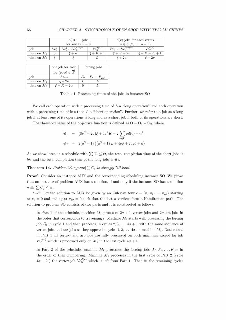
56 CHAPTER 4. SYNCHRONOUS OPEN SHOP WITH TWO MACHINES
d(0) + 1 jobs d(v) jobs for each vertexfor vertex v = 0 v ∈ 1, 2, . . . , n− 1
job Ve00 Ve10 · · ·Ved(0)−10 Ve
d(0)0 Ve1v · · · Ve
d(v)−1v Ve
d(v)v
time on M1 0 ξ +K ξ +K + 1 ξ +K − 2v ξ +K − 2v + 1
time on M2 ξ ξ L ξ + 2v ξ + 2v
one job for each forcing jobs
arc (v, w) ∈ −→Ejob Arvw F0 F1 · · ·F2n9
time on M1 ξ + 2v L L
time on M2 ξ +K − 2w 0 L
Table 4.1: Processing times of the jobs in instance SO
We call each operation with a processing time of L a “long operation” and each operation
with a processing time of less than L a “short operation”. Further, we refer to a job as a long
job if at least one of its operations is long and as a short job if both of its operations are short.
The threshold value of the objective function is defined as Θ = Θ1 + Θ2, where
Θ1 = (8σ2 + 2σ)ξ + 4σ2K − 2∑v∈V
vd(v) + n2,
Θ2 = 2(n9 + 1)((n9 + 1
)L+ 4σξ + 2σK + n
).
As we show later, in a schedule with∑Cj ≤ Θ, the total completion time of the short jobs is
Θ1 and the total completion time of the long jobs is Θ2.
Theorem 14. Problem O2|synmv|∑Cj is strongly NP-hard.
Proof: Consider an instance AUX and the corresponding scheduling instance SO. We prove
that an instance of problem AUX has a solution, if and only if the instance SO has a solution
with∑Cj ≤ Θ.
“⇒”: Let the solution to AUX be given by an Eulerian tour ε = (v0, v1, . . . , v2σ) starting
at v0 = 0 and ending at v2σ = 0 such that the last n vertices form a Hamiltonian path. The
solution to problem SO consists of two parts and it is constructed as follows:
– In Part 1 of the schedule, machine M1 processes 2σ + 1 vertex-jobs and 2σ arc-jobs in
the order that corresponds to traversing ε. Machine M2 starts with processing the forcing
job F0 in cycle 1 and then proceeds in cycles 2, 3, . . . , 4σ + 1 with the same sequence of
vertex-jobs and arc-jobs as they appear in cycles 1, 2, . . . , 4σ on machine M1. Notice that
in Part 1 all vertex- and arc-jobs are fully processed on both machines except for job
Ved(v)0 which is processed only on M1 in the last cycle 4σ + 1.
– In Part 2 of the schedule, machine M1 processes the forcing jobs F0, F1, . . . , F2n9 in
the order of their numbering. Machine M2 processes in the first cycle of Part 2 (cycle
4σ + 2 ) the vertex-job Ved(v)0 which is left from Part 1. Then in the remaining cycles

4.3. MINIMIZING THE TOTAL COMPLETION TIME 57
4σ + 3, . . . , 4σ + 2 + 2n9, every job Fi (i = 1, . . . , 2n9) on M1 is paired with job Fi+1 on
M2 if i is odd, and with job Fi−1, otherwise.
In Fig. 4.16 we present an example of the described schedule based on graph−→G of Fig. 4.15.
Notice that there are n = 5 vertices in−→G , and parameter σ equals 8. Traversing the Eulerian
tour ε = (0, 1, 0, 2, 0, 3, 0, 4, 2, 4, 3, 2, 1, 2, 3, 4, 0 ) incurs the sequence of vertex-jobs and arc-jobs
(Ve00, Ar01, Ve1
1, Ar10, Ve10, Ar02, . . ., Ve2
1, Ar12, Ve42, Ar23, Ve3
3, Ar34, Ve43, Ar40, Ve4
0). There
are 2σ + 1 = 17 vertex-jobs, 2σ = 16 arc-jobs and 2n9 + 1 = 2 · 59 + 1 jobs Fi, so that all jobs
are allocated in 34 + 2 · 59 cycles. The schedule is represented as a sequence of cycles, where
the operations on machines M1 and M2 are enframed and the lengths of the corresponding
operations are shown above or below. Operations of equal length in one cycle are shown as two
boxes of the same length; the sizes of the boxes of different cycles are not to scale.
We demonstrate that the constructed schedule satisfies∑Cj = Θ. Observe that most
cycles have equal workload on both machines, except for the n cycles that correspond to the
vertex-jobs of the Hamiltonian path; in each such cycle the operation on M1 is one unit longer
than the operation on M2.
First consider the short jobs. The initial vertex-job Ve00 that corresponds to the origin v0 = 0
of ε = (v0, v1, . . . , v2σ) completes at time ξ. Each subsequent vertex-job that corresponds to
vi, 1 ≤ i ≤ 2σ − n, where we exclude the last n vertices of the Hamiltonian path, completes
at time (2i + 1)ξ + iK. Consider the next n − 1 vertex-jobs vi with 2σ − n + 1 ≤ i ≤ 2σ − 1
(excluding the very last vertex-job Ved(0)0 as it is a long job); every such job vi completes at
time (2i+ 1)ξ + iK + (n+ i− 2σ).
The remaining short jobs correspond to arc-jobs. The completion time of the i-th arc-job
Arvi−1vi is 2iξ+iK−2vi for 1 ≤ i ≤ 2σ−n and 2iξ+iK−2vi+(n+i−2σ) for 2σ−n+1 ≤ i ≤ 2σ.
Thus, the total completion time of all short jobs sums up to
ξ +
2σ−n∑i=1
[(2i+ 1)ξ + iK] +
2σ−1∑i=2σ−n+1
[(2i+ 1)ξ + iK + (n+ i− 2σ)]
+
2σ−n∑i=1
[2iξ + iK − 2vi] +
2σ∑i=2σ−n+1
[2iξ + iK − 2vi + (n+ i− 2σ)]
=
[ξ +
2σ−1∑i=1
(2i+ 1)ξ +
2σ∑i=1
2iξ
]+
[2σ−1∑i=1
iK +
2σ∑i=1
iK
]+
[n−1∑i=1
i+
n∑i=1
i
]− 2
2σ∑i=1
vi
=(8σ2 + 2σ)ξ + 4σ2K + n2 − 2∑v∈V
vd(v) = Θ1.
Here we have used the equality
2σ∑i=1
vi =∑v∈V
vd(v)

58 CHAPTER 4. SYNCHRONOUS OPEN SHOP WITH TWO MACHINES
Part 1:Cycle 1
0Ve0
0
F0
0
Cycle 2
ξAr01
Ve00
ξ︸ ︷︷ ︸ξ
Cycle 3
ξ+K−2
Ve11
Ar01
ξ+K−2
Cycle 4
ξ+2
Ar10
Ve11
ξ+2︸ ︷︷ ︸2ξ+K
Cycle 5
ξ+K
Ve10
Ar10
ξ+K
Cycle 6
ξ
Ar02
Ve10
ξ︸ ︷︷ ︸2ξ+K
Cycle 7
ξ+K−4
Ve12
Ar02
ξ+K−4
Cycle 8
ξ+4
Ar20
Ve12
ξ+4︸ ︷︷ ︸2ξ+K
Cycle 9
ξ+K
Ve20
Ar20
ξ+K
Cycle 10
ξ
Ar03
Ve20
ξ︸ ︷︷ ︸2ξ+K
Cycle 11
ξ+K−6
Ve13
Ar03
ξ+K−6
Cycle 12
ξ+6
Ar30
Ve13
ξ+6︸ ︷︷ ︸2ξ+K
Cycle 13
ξ+K
Ve30
Ar30
ξ+K
Cycle 14
ξ
Ar04
Ve30
ξ︸ ︷︷ ︸2ξ+K
Cycle 15
ξ+K−8
Ve14
Ar04
ξ+K−8
Cycle 16
ξ+8
Ar42
Ve14
ξ+8︸ ︷︷ ︸2ξ+K
Cycle 17
ξ+K−4
Ve22
Ar42
ξ+K−4
Cycle 18
ξ+4
Ar24
Ve22
ξ+4︸ ︷︷ ︸2ξ+K
Cycle 19
ξ+K−8
Ve24
Ar24
ξ+K−8
Cycle 20
ξ+8
Ar43
Ve24
ξ+8︸ ︷︷ ︸2ξ+K
Cycle 21
ξ+K−6
Ve23
Ar43
ξ+K−6
Cycle 22
ξ+6
Ar32
Ve23
ξ+6︸ ︷︷ ︸2ξ+K
Cycle 23
ξ+K−4
Ve32
Ar32
ξ+K−4
Cycle 24
ξ+4
Ar21
Ve32
ξ+4︸ ︷︷ ︸2ξ+K
Cycle 25
ξ+K−1
Ve21
Ar21
ξ+K−2
Cycle 26
ξ+2
Ar12
Ve21
ξ+2︸ ︷︷ ︸2ξ+K+1
Cycle 27
ξ+K−3
Ve42
Ar12
ξ+K−4
Cycle 28
ξ+4
Ar23
Ve42
ξ+4︸ ︷︷ ︸2ξ+K+1
Cycle 29
ξ+K−5
Ve33
Ar23
ξ+K−6
Cycle 30
ξ+6
Ar34
Ve33
ξ+6︸ ︷︷ ︸2ξ+K+1
Cycle 31
ξ+K−7
Ve34
Ar34
ξ+K−8
Cycle 32
ξ+8
Ar40
Ve34
ξ+8︸ ︷︷ ︸2ξ+K+1
Cycle 33=4σ + 1
ξ+K+1
Ve40
Ar40
ξ+K︸ ︷︷ ︸ξ+K+1
Part 2:4σ + 2
Cycle 34
L
F0
Ve40
L︸ ︷︷ ︸L
Cycle 35
L
F1
F2
L
Cycle 36
L
F2
F1
L︸ ︷︷ ︸F1,F2 pair of length 2L
Cycle 35
L
F3
F4
L
Cycle 36
L
F4
F3
L︸ ︷︷ ︸F3,F4 pair of length 2L
· · ·Cycle 34+2·59-1
L
F2n9−1
F2n9
L
4σ + 2 + 2 · n9
Cycle 34+2·59L
F2n9
F2n9−1
L︸ ︷︷ ︸F2n9−1,F2n9 pair of length 2L
Figure 4.16: An optimal solution to SO

4.3. MINIMIZING THE TOTAL COMPLETION TIME 59
which holds for the Eulerian tour ε = (v0, v1, . . . , v2σ) with vi ∈ V .
Next, consider the completion times of the long jobs. The second operations of jobs Ved(0)0
and F0 appear in cycle 4σ+ 2; all other long operations are scheduled in cycles 4σ+ 3, . . . , 4σ+
2 + 2n9. There is a common part of the schedule, with cycles 1, 2, . . . , 4σ + 1 that contributes
to the completion time of every long job; the length of that common part is
∆ = 4σξ + 2σK + n.
Then the first two long jobs, F0 and Ved(0)0 , are both completed at time ∆ + L and for i =
1, . . . , n9 the completion time of each pair of jobs F2i−1 and F2i is ∆ + (2i + 1)L. Thus, the
total completion time of the long jobs sums up to
2 (∆ + L) + 2
n9∑i=1
[∆ + (2i+ 1)L] (4.15)
= 2∆(n9 + 1) + 2(n9 + 1)2L (4.16)
= 2(n9 + 1)[(4σξ + 2σK + n) + (n9 + 1)L] = Θ2 (4.17)
and therefore the total completion time sums up to Θ = Θ1 + Θ2.
“⇐”: Now we prove that if an instance of AUX does not have a solution, then also SO does
not have a solution with∑Cj ≤ Θ. Suppose to the contrary that there exists a schedule with∑
Cj ≤ Θ and let S be an optimal schedule. Such a schedule satisfies the following structural
properties (the proof is again moved to the next section).
1. In each cycle in S, both operations are either short or long.
2. All long operations are scheduled in the last 2n9 + 1 cycles. This defines the splitting of
schedule S into Parts 1 and 2, with cycles 1, 2, . . . , 4σ + 1 and 4σ + 2, . . . , 4σ + 2 + 2n9.
3. The sum of completion times of all long jobs is at least Θ2.
4. In S, machine M1 operates without idle times.
5. In Part 1 of S, job Ve00 is processed in the first two cycles which are of the form
Ve00
F0
∗Ve0
0
, where ∗ represents a short operation. While the order of these two cycles is
immaterial, without loss of generality we assume thatVe0
0
F0
precedes∗
Ve00
; otherwise
the cycles can be swapped without changing the value of∑Cj .
6. The two operations of each vertex-job and the two operations of each arc-job are processed
in two consecutive cycles, first on M1 and then on M2.

60 CHAPTER 4. SYNCHRONOUS OPEN SHOP WITH TWO MACHINES
7. In Part 1 of S, machine M1 alternates between processing arc-jobs and vertex-jobs. More-
over, an operation of a vertex-job corresponding to v is followed by an operation of an
arc-job corresponding to an arc leaving v. Similarly, an operation of an arc-job for arc
(v, w) is followed by an operation of a vertex-job for vertex w.
By Property 6, the same is true for machine M2 in Part 1 and in the first cycle that
follows it.
8. The first arc-job that appears in S corresponds to an arc leaving 0. Among the vertex-jobs,
the last one is Ved(0)0 .
Using the above properties we demonstrate that if problem AUX does not have a solution,
then the value of∑Cj in the optimal schedule S exceeds Θ. Due to Property 3 it is sufficient
to show that the total completion time∑µj=1 Cj of all short jobs exceeds Θ1. Let us assume
that 1, 2, . . . , µ with µ = 4σ are the short jobs of the instance SO. This set consists of 2σ
short vertex-jobs (the long vertex-job Ved(0)0 is excluded) and 2σ arc-jobs.
Properties 1-2 allow the splitting of S into two parts. Part 2 plays an auxiliary role. Part 1
is closely linked to problem AUX.
The sequence of arc- and vertex-jobs in Part 1 of S defines an Eulerian tour in−→G . Indeed,
all arc-jobs appear in S and by Property 7 the order of the arc- and vertex-jobs in S defines an
Eulerian trail in−→G . Since for every vertex v, its in-degree equals its out-degree, an Eulerian
trail must be an Eulerian tour. Denote it by ε = (v0, v1, . . . , v2σ). Due to Property 8 and by
the assumption of Property 5 the Eulerian tour ε starts and ends at v0 = 0.
In Fig. 4.17 we present the structure of Part 1 of schedule S, where Ve∗v represents one of
the vertex-jobs Ve1v, Ve2
v,. . . , Ved(v)v , with processing time ξ + K − 2v + 1 or ξ + K − 2v on
machine M1, depending on whether the upper index is d(v) or a smaller number. Part 2 is as
in the proof of “ ⇒”.
Part 1:Cycle 1
0
Ve00
F0
0
Cycle 2
ξ
Ar0v1
Ve00
ξ︸ ︷︷ ︸ξ
Cycle 3
ξ+K−2v1(+1)
Ve∗v1Ar0v1
ξ+K−2v1
Cycle 4
ξ+2v1
Arv1v2Ve∗v1ξ+2v1︸ ︷︷ ︸
2ξ+K(+1)
Cycle 5
ξ+K−2v2(+1)
Ve∗v2Arv1v2ξ+K−2v2
Cycle 6
ξ
Arv2v3Ve∗v2ξ︸ ︷︷ ︸
2ξ+K(+1)
. . .
Cycle 4σ − 1
ξ+K−2v2σ−1(+1)
Ve∗v2σ−1
Arv2σ−2v2σ−1
ξ+K−2v2σ−1
Cycle 4σ
ξ+2v2σ−1
Arv2σ−10
Ve∗v2σ−1
ξ+2v2σ−1︸ ︷︷ ︸2ξ+K(+1)
Cycle 4σ + 1
ξ+K+1
Ved(0)0
Arv2σ−10
ξ+K︸ ︷︷ ︸ξ+K+1
Figure 4.17: Structure of schedule S

4.3. MINIMIZING THE TOTAL COMPLETION TIME 61
Notice that all operations of the short jobs appear only in Part 1 of the above schedule, with
one short job completing in each cycle 2, 3, . . . , µ+1. In each cycle of Part 1, both operations are
of the same length, except for the n−1 cycles where the vertex-jobs Ved(v)v , v ∈ 1, 2, . . . , n−1,
are scheduled on machine M1, and the final cycle of Part 1 where Ved(0)0 is scheduled. In these
cycles the operation on M1 is one unit longer than the operation on M2. Let
ϑ :=
Ved(v)v | v = 1, 2, . . . , n− 1
be the set of the n− 1 jobs with one extra unit of processing. Job Ve
d(0)0 is not included in this
set as its precise location is known by Property 8.
We show that for any Eulerian tour ε = (v0, v1, . . . , v2σ), the value of∑µj=1 Cj does not
depend on the order of the vertices in ε; it only depends on the positions of the n− 1 jobs from
ϑ. In particular, we demonstrate that
µ∑j=1
Cj = Υ +
µ+1∑`=2
(µ− `+ 2)x`, (4.18)
where Υ = Θ1−n2 is a constant, and x` ∈ 0, 1 indicates whether some job from ϑ is allocated
to cycle ` or not.
The constant term Υ is a lower bound estimate for∑µj=1 Cj obtained under the assumption
that one additional time unit for each job from ϑ and also for job Ved(0)0 is ignored. If we drop
“+1” from the input data of the instance SO, then both machines have equal workload in every
cycle. Job Ve00 contributes ξ to Υ. The job corresponding to vi, except for job Ve
d(0)0 (which
is a long job) contributes (2i + 1)ξ + iK. The arc-job corresponding to (vi, vi+1) contributes
2iξ + iK − 2vi+1. Thus,
Υ = ξ +
2σ−1∑i=1
[(2i+ 1)ξ + iK] +
2σ∑i=1
[2iξ + iK − 2vi+1]
= (8σ2 + 2σ)ξ + 4σ2K − 2∑v∈V
vd(v) = Θ1 − n2.
Consider now the effect of the additional time unit on machine M1 for each job from ϑ and
for job Ved(0)0 . If some ϑ-job is allocated to a cycle `, then the additional unit of processing
increases by one the completion time of every short job finishing in cycles `, ` + 1, . . . , µ + 1,
and thus contributes (µ+ 1)− `+ 1 to∑µj=1 Cj . This justifies formula (4.18).
As shown in the above template, each of the n− 1 jobs j ∈ ϑ can be scheduled in any odd-
numbered cycle ` ∈ 3, 5, . . . , µ− 1. Also, by Property 8, an additional time unit appears in
cycle µ+ 1 due to the allocation of Ved(0)0 to machine M1, which affects the completion time of
a short job in that cycle. Thus, the minimum value of∑µj=1 Cj is achieved if all n−1 jobs from
ϑ are allocated to the latest possible odd-numbered positions, i.e., to positions ` = (µ− 1)− 2i

62 CHAPTER 4. SYNCHRONOUS OPEN SHOP WITH TWO MACHINES
for i = 0, 1, . . . , n − 2. Together with an extra “1” related to the allocation of Ved(0)0 to cycle
µ+ 1, this results in
µ+1∑`=2
(µ− `+ 2)x` = 1 +
n−2∑i=0
[µ− (µ− 1− 2i) + 2]
= 1 + 3 + · · ·+ (2n− 1) = n2,
so that∑µj=1 Cj is equal to Θ1 if jobs ϑ are allocated to the latest feasible positions. Due
to (4.18), any other allocation of jobs ϑ, which does not involve the last n − 1 odd-numbered
positions, results in a larger value of∑µj=1 Cj .
By the main assumption of the part “⇐”, AUX does not have a solution where the last
n vertices form a Hamiltonian path. Therefore, the last n vertices of any Eulerian tour ε =
(v0, v1, . . . , v2σ) have at least two occurrences of the same vertex v and therefore in the associated
schedule, among the last n vertex-jobs there are at least two vertex-jobs Veiv, Vejv associated
with v. Thus, it is impossible to have n−1 jobs from ϑ allocated to the last n−1 odd-numbered
cycles and to achieve the required threshold value Θ1.
At the end of this section we observe that the proof of Properties 1 – 8 can be adjusted
to handle the case with dummy jobs. Indeed, in an optimal solution of the instance, even if
we allow dummy jobs, dummy operations are not allowed to be paired with actual operations
of non-zero length (see Property 4). We conclude therefore that the complexity status of the
relaxed problem is the same as that for the standard one.
Theorem 15. Problem O2|synmv, rel|∑Cj is strongly NP-hard.
4.4 Details for the NP-hardness of O2|synmv|∑Cj
In this section we work out the details of the NP-hardness proof for problem O2|synmv|∑Cj
that were left out in Section 4.3.
We first show that the HAMILTONIAN PATH problem and its modification AUX from
the previous section have the same complexity status. Recall the definitions from graph theory
introduced in Section 2.1. For completeness, let us briefly repeat the construction of graph−→G needed for problem AUX. We start out with a connected graph G′ = (V ′, E′) with V ′ =
1, 2, . . . , n − 1. To construct the graph−→G for problem AUX, we first construct the graph
G = (V,E) by adding a universal vertex 0 which is connected by an edge with every vertex. In
a second step, we construct a directed graph−→G = (V,
−→E ) by replacing each edge v, w ∈ E by
two directed edges (v, w) and (w, v), one in each direction. Note that in−→G we have deg−−→
G(v) =
deg+−→G
(v) for all v ∈ V by construction, i.e.−→G is Eulerian.
Lemma 16. The following statements are equivalent.

4.4. DETAILS FOR THE NP-HARDNESS OF O2|SY NMV |∑CJ 63
(1) There exists a Hamiltonian path in G′.
(2) There exists a Hamiltonian path in G ending in 0.
(3) There exists a directed Hamiltonian path in−→G ending in 0.
(4) There exists an Eulerian tour in−→G , starting and ending in 0, such that the last n vertices
form a Hamiltonian path.
Proof: The implications (1)⇒ (2)⇒ (3) are obvious. We prove that (3)⇒ (4). Suppose there
exists a Hamiltonian path h = (v0, v1, . . . , vn−1) in−→G with vn−1 = 0. Then create a graph
−→G∗ by removing from
−→G all arcs that appear in h. By the properties of vertex 0, graph
−→G∗ is
still strongly connected. Furthermore, for each inner vertex v1, v2, . . . , vn−2 of h, its in-degree
in−→G∗ still equals its out-degree, as one entering and one leaving edge is removed for each of
them. Lastly note that for vn−1 = 0 we have deg+−→G∗
(0) = deg−−→G∗
(0) + 1, as an arc entering 0 is
removed, but not a leaving one. Similarly, for v0, deg−−→G∗
(v0) = deg+−→G∗
(v0) + 1, as an arc leaving
v0 is removed, but not the one entering v0.
We conclude that−→G∗ contains an Eulerian trail ε∗, that starts in 0 and ends in v0. Then the
concatenation ε = ε∗ h starts and ends in 0 and its last n vertices form a Hamiltonian path h.
It remains to prove (4) ⇒ (1). Let ε be an Eulerian tour in−→G , starting and ending in 0,
such that the last n vertices form a Hamiltonian path, and let that path be h = (v0, v1, ..., vn−1)
with vn−1 = 0. Notice that the vertex 0 appears only once in h. Then h∗ = (v0, v1, ..., vn−2) is
a path in G. Since h∗ consists of all n− 1 vertices of G, h∗ is a Hamiltonian path in G′.
Therefore G′ is a yes-instance of the HAMILTONIAN PATH problem if and only if−→G is a
yes-instance for problem AUX and the two problems have the same complexity status.
The remainder of this section deals with Properties 1-8 from the proof of Theorem 14.
These properties characterize the structure of an optimal schedule S for instance SO, under the
assumption that∑Cj ≤ Θ for that schedule.
Lemma 17. An optimal schedule S for instance SO with∑Cj ≤ Θ satisfies Properties 1-8.
Proof: Property 1: In each cycle in S, both operations are either short or long.
Assume the opposite and let s be the first cycle that contains a short and a long operation.
Since the number of long operations is even, there is at least one further cycle t which contains
operations of both types and in which the long operation is on a different machine than in cycle
s. In the following, assume that long operations are on machine M2 in cycle s and on machine
M1 in cycle t; the alternative case is similar. Let Js and js be the jobs in cycle s, with the
operation of Js being long and the operation of js being short. Let Jt and jt be the jobs in
cycle t, with the operation of Jt being long and the operation of jt being short.
Assume first that Js 6= Jt and js 6= jt. Construct a new schedule S′ by swapping the
operations on M2, see Fig. 4.18. Then, the length of cycle s in S′ decreases by at least

64 CHAPTER 4. SYNCHRONOUS OPEN SHOP WITH TWO MACHINES
L− (ξ+K+ 1) while all other cycles keep their lengths unchanged. The completion time of job
Js either decreases, if its second operation is in cycle after t, or it increases by at most (ξ+K+1)
plus the total length of cycles s+ 1, . . . , t. Thus, C ′Js −CJs ≤ (t− s− 1)L+ (ξ+K+ 1). For all
other jobs that finish in cycle s or later, the completion times decrease by at least L−(ξ+K+1).
As there are at least t− s+ 1 cycles in the tail part of the schedule, starting from cycle s, this
affects at least t− s+ 1 jobs. Thus, the difference in total completion time is∑j∈N
(C ′j − Cj) ≤ (t− s− 1)L+ (ξ +K + 1) +∑
j∈N\Js(C ′j − Cj)
≤ (t− s− 1)L+ (ξ +K + 1)
−(t− s+ 1)(L− (ξ +K + 1))
< −2L+ |N |(ξ +K + 1),
where |N | is the number of jobs in the instance SO or equivalently the number of cycles. To
show that we get an improved solution S′, we prove that
−2L+ |N |(ξ +K + 1) < 0 (4.19)
using the estimate on σ = |−→E |/2,
n ≤ σ < n2 (for n > 2), (4.20)
combined with the definitions of |N |, ξ, L and K:
K = 8n, (4.21)
|N | = 2n9 + 4σ + 2 ≤ 2n9 + 4n2 + 2, (4.22)
ξ = 4Kσ2 = 32nσ2 < 32n5, (4.23)
L = 2n9ξ = 2n9 · 32nσ2 ≥ 64n12 > 576n10 (for n > 3). (4.24)
Indeed,
−2L+ |N |(ξ +K + 1) ≤≤ −2n9ξ + 2n9(K + 1) + (4σ + 2)(ξ +K + 1)
< −576n10 + 2n9(8n+ 1)
+(4n2 + 4)(32n5 + 8n+ 1)
< −576n10 + 18n10 + 8n2 · 41n5 < 0.
Thus, swapping the operations leads to a smaller total completion time, contradicting that S
has minimal total completion time.

4.4. DETAILS FOR THE NP-HARDNESS OF O2|SY NMV |∑CJ 65
M1
M2 Js
js · · · Jt
jt
js
jt
· · · Jt
Js
L L
L≤ ξ +K + 1
M1
M2
⇓≤ (t− s− 1)L
s t
s t
· · · · · ·
· · · · · ·
Figure 4.18: Creating a cycle of long operations and a cycle of short operations if Js 6= Jt andjs 6= jt
Consider the case Js = Jt, js 6= jt and assume first that there are other long operations
scheduled before s. The case where there is no other long operation scheduled prior to cycle s
is discussed afterwards. Let r be the last cycle before s in which a long operation is scheduled,
r < s. Since s is the first cycle that contains a short as well as a long operation, both operations
in cycle r are long. In this case construct S′ by exchanging in cycles r, s and t the three
operations on machine M2, as shown in Fig. 4.19(a). As a result, the completion time of job
Jr either decreases, if the last operation of that job is in a cycle after cycle t, or it increases by
at most (s− r)(ξ+K+ 1) + (t− s)L, where the first term represents the estimate on the length
of short cycles r+ 1, . . . , s in S′ and the second term estimates the length of cycles s+ 1, . . . , t,
which may be short or long. For all other jobs, including job Js, that finish in cycle s or later,
their completion times decrease by at least L− (ξ+K+1). Note that there are at least t−s+2
such jobs. Thus, ∑j∈N
(C ′j − Cj) ≤ [(s− r)(ξ +K + 1) + (t− s)L]
−(t− s+ 2)(L− (ξ +K + 1))
= −2L+ (t− r + 2)(ξ +K + 1) < 0,
where the last inequality can be proved as a slight modification of (4.19).
Assume now that there is no long operation scheduled prior to cycle s and let u > s be
the first cycle that contains a long operation of some job Ju on the same machine as the long

66 CHAPTER 4. SYNCHRONOUS OPEN SHOP WITH TWO MACHINES
operation in cycle t. Construct S′ by swapping the M1-operations in cycles t and u and the
M2-operations in cycles s and t, see Fig. 4.19(b) for an example with u > t. The completion
time of job Js (or job Ju if s < u < t) increases by at most |u − t|L. For the remaining jobs
scheduled in the tail part of the schedule, starting from cycle s, their completion times reduce
by at least L− (ξ+K + 1). Again, using the evaluation from above, this leads to a decrease in
the total completion time,∑j∈N
(C ′j − Cj) ≤ |u− t|L− (max u, t − s+ 1) (L− (ξ +K + 1))
= − (min u, t − s+ 1)L
+ (max u, t − s+ 1) (ξ +K + 1)
≤ −2L+ |N | (ξ +K + 1)(4.19)< 0.
In all previous cases a better schedule S′ is constructed by grouping two short operations
js and jt in one cycle. Next, consider js = jt and first assume that there are other short
operations scheduled in some cycle r < s. Since s is the first cycle that contains a short as well
as a long operation, both operations in cycle r are short. Construct a schedule S′ as illustrated
in Fig. 4.20(a). Then, the completion time of job js decreases by at least 2(L − (ξ + K + 1)),
as both its operations were paired with long operations before and are now paired with short
ones. Further, the completion times of all jobs that were completed in cycles r, r+ 1, . . . , t− 1
in S, increase by at most (ξ +K + 1) and the completion times of all jobs that are completed
in cycle t or later decrease by at least L− (ξ +K + 1). Thus,∑j∈N
(C ′j − Cj) ≤ −2(L− (ξ +K + 1)) + (t− r)(ξ +K + 1)
− (L− (ξ +K + 1))
< −3L+ (t− r + 3)(ξ +K + 1) < 0,
where the last inequality can be proved similar to (4.19).
Consider now the case where r > s and assume additionally that both operations in cycle
r are short (see Fig. 4.20(b) for an example of r > t > s). In this case, the completion times
of job js and all jobs that finish in cycle s or later, except for job Js, decrease by at least
L − 2(ξ + K + 1). The completion time of job js decreases further by the total length ∆ of
cycles s+1, . . . , t−1, while the completion time of job Js may increase by at most 2(ξ+K+1)

4.4. DETAILS FOR THE NP-HARDNESS OF O2|SY NMV |∑CJ 67
M1
M2 Js
js Js
jt
s
· · ·
Jr
r
≤ (s− r − 1)(ξ +K + 1)
M1
M2
js Js
Jr
s t
· · ·
Js
r
· · ·
⇓
jt
M1
M2 Js
js Js
jt
s t
· · ·
u
M1
M2
js Ju
Js
s t
· · ·
⇓
jt
≤ (u− t− 1)L
Ju· · ·
· · · Js
u
(a)
(b)
· · ·· · · · · ·
· · · · · ·
∗
∗
∗
∗
· · · · · ·
· · · · · ·
Figure 4.19: Creating a cycle of long operations and a cycle of short operations if Js = Jt,js 6= jt and(a) there is a long operation in cycle r, r < s,(b) there is no long operation in any cycle r, r < s, but there is a long operation in cycle u,u > s
plus ∆, again leading to a decrease in the total completion time:∑j∈N
(C ′j − Cj) ≤ −((maxt, r − s) · (L− 2(ξ +K + 1))−∆
+2(ξ +K + 1) + ∆
≤ −2(L− 2(ξ +K + 1)) + 2(ξ +K + 1)
= −2L+ 6(ξ +K + 1)(4.19)< 0,
where the last inequality follows from (4.19) since 6 < |N | = 2n9 + 4σ + 2.
The only remaining case with js = jt is where no cycle r exists such that both operations
in r are short, i.e., all short operations are paired with long operations. In this case, for cycle
s with a short operation on M1 and a long operation on M2, we select a cycle t′ similar to t,

68 CHAPTER 4. SYNCHRONOUS OPEN SHOP WITH TWO MACHINES
M1
M2 Js
js Jt
js
s t
· · ·jr1
jr2
r
· · ·
⇓M1
M2
s+ 1 t
· · ·
r
· · · x
M1
M2
s t
· · ·
r
· · ·
⇓
M1
M2
t+ 1 r
· · ·
s
· · · x
y
(a)
(b)
jr1 js
js jr2
Jt
Js y
js Jt
Js js
jr1
jr2
jr1 js
js jr2
Jt
Js
· · · · · ·
t− 1
x
y
· · ·· · ·
r − 1
x
y· · · · · ·
· · ·· · ·
r + 1
s+ 1
Figure 4.20: Creating a cycle of long operations and a cycle of short operations if Js 6= Jt,js = jt and there is a cycle r with two short operations,(a) r < s,(b) r > s
with a short operation on M2 and a long operation on M1, t′ 6= t (such a cycle always exists
for n > 2). Then the two short operations in cycles s and t′ belong to different jobs, and the
case reduces to one of the cases with js 6= jt considered before.
In case that js = jt and Js = Jt we can first swap one of the long operations with a long
operation in another cycle, as described for Js = Jt, and afterwards continue with moving the
two short operations to the front of the schedule, as described for js = jt, again leading to
a decrease in the total completion time. Therefore, in an optimal schedule there is no cycle
consisting of a long and a short operation.
Property 1 is proved. From now on we refer to cycles as short or long assuming that there
are no “mixed cycles” in an optimal schedule.
Property 2: All long operations are scheduled in the last 2n9 + 1 cycles. This defines the
splitting of schedule S into Parts 1 and 2, with cycles 1, 2, . . . , 4σ+1 and 4σ+2, . . . , 4σ+2+2n9.
Let U = (s + 1, . . . , t) be the last sequence of short cycles and let s be a long cycle that
precedes U . Assume first that |U | ≥ 2. Then, as cycles in U are the last short cycles, at least
|U | − 1 jobs finish within U (U may contain the two short operations of jobs Ved(0)0 and F0 for

4.4. DETAILS FOR THE NP-HARDNESS OF O2|SY NMV |∑CJ 69
which their respective second, long operations may be scheduled in later cycles). Construct a
schedule S′ by moving the long cycle s after U , see Fig. 4.21. Then the completion times of at
least |U | − 1 jobs decrease by L while the completion times of the two jobs scheduled in cycle
s in S increase by at most |U | (ξ +K + 1),∑j∈N
(C ′j − Cj) ≤ − (|U | − 1)L+ 2 |U | (ξ +K + 1)
= L− |U | (L− 2(ξ +K + 1)) .
Using conditions |U | ≥ 2 and L − 2(ξ + K + 1) > 0 (which can be proved in the same way as
(4.19)) we deduce∑j∈N
(C ′j − Cj) ≤ L− 2 (L− 2(ξ +K + 1)) = −L+ 4(ξ +K + 1) .
The last expression is negative, again by the same arguments as (4.19). Thus, we get a contra-
diction to the optimality of S.
If |U | = 1 and the short cycle in U is different from
ξ +K + 1
Ved(0)0
F0
0︸ ︷︷ ︸ξ+K+1
(4.25)
then at least one job, different from Ved(0)0 and F0, finishes in U . In this case the previous
transformation reduces the completion time of at least one job by L, while the completion
times of the two jobs scheduled in cycle s in S increase by at most (ξ +K + 1),∑j∈N
(C ′j − Cj) ≤ −L+ 2(ξ +K + 1) < 0,
where the last inequality can be proved in the same way as (4.19).
Consider now the case with U consisting of only one short cycle of the form (4.25). Notice
that such a cycle is avoided in the optimal solution presented in Fig. 4.16.
Let U be the last sequence of short cycles before U and assume first that U is preceded by
some long cycles. Clearly U does not contain short operations of jobs F0 and Ved(0)0 , as they
appear in U . Since no other job consists of both, long and short operations, at least |U | short
jobs finish within U . Then the arguments presented in the beginning of the proof of Property 2
are applicable for the set of cycles U used instead of U .
Lastly, consider the remaining case with U consisting of only one short cycle of the form
(4.25) and there are no other short cycles in the preceding part of the schedule that follow

70 CHAPTER 4. SYNCHRONOUS OPEN SHOP WITH TWO MACHINES
M1
M2 Js2
Js1 J(s+1)1
J(s+1)2
s s+ 1
Jt1
Jt2
t
· · ·
⇓
M1
M2
s t− 1
· · ·
t
J(s+1)1
J(s+1)2
Jt1
Jt2
Js1
Js2
· · · · · ·
· · · · · ·
Figure 4.21: Moving long cycle s after a sequence of short cycles U = s+ 1, . . . , t
a long cycle. Then, the first 4σ cycles are short and the cycle (4.25) appears among the last
2(n9+1) cycles. Using pairwise interchange arguments it is easy to make sure that in an optimal
schedule, the latter cycles are of the form shown in Fig. 4.22, where without loss of generality
jobs Fi, except for F0, are renumbered in the order they appear in schedule S on machine M1.
· · · F1
F2
F2
F1︸ ︷︷ ︸F1,F2 pairof length 2L
F3
F4
F4
F3︸ ︷︷ ︸F3,F4 pairof length 2L
· · · Fτ−1
Fτ
FτFτ−1︸ ︷︷ ︸
Fτ−1,Fτ pair
of length 2L
Ved(0)0
F0
F0
Ved(0)0︸ ︷︷ ︸
Ved(0)0 ,F0 pair
of length (ξ+K+1)+L
Fτ+1
Fτ+2
Fτ+2
Fτ+1︸ ︷︷ ︸Fτ+1,Fτ+2 pair
of length 2L
· · ·
F2n9−1
F2n9
F2n9
F2n9−1︸ ︷︷ ︸F2n9−1
,F2n9 pair
of length 2L
Figure 4.22: A special short cycle appearing among the last 2(n9 + 1) cycles
In Fig. 4.22, τ is the number of jobs from the set F1, F2, ..., F2n9 completed before cycle
(4.25), 1 ≤ τ ≤ 2n9. Let ∆ be the total length of the first 4σ short cycles. If the length of cycle
(4.25) was L, then the total completion time of all long jobs would be
2(n9 + 1)∆ + 2L
n9+1∑i=1
2i = 2(n9 + 1)(∆ + (n9 + 2)L
).
In reality, the length of cycle (4.25) is less than L by the amount L − (ξ +K + 1), so that
completion times of the jobs that appear after Fτ−1, Fτ should be adjusted. The number of

4.4. DETAILS FOR THE NP-HARDNESS OF O2|SY NMV |∑CJ 71
jobs completed in the corresponding tail part of the schedule is 2(n9 + 1)− τ , so that∑long jobs
Cj = 2(n9 + 1)(∆ + (n9 + 2)L
)−(2(n9 + 1)− τ)(L− ξ −K − 1)
= 2(n9 + 1)((n9 + 1)L+ ∆ + ξ +K + 1
)+τ(L− ξ −K − 1) .
We demonstrate that the objective value for schedule S exceeds the given threshold Θ, using
the estimate (4.20) together with the following conditions:
∆ ≥ 4σξ + 2σK,
L− ξ −K − 1 > 0,
where the first one is a lower bound on ∆ calculated as the sum of processing times on the
second machine of the short operations in the first 4σ cycles (which includes every operation
except the zero-length operation of job F0), while the second one can be proved in a similar
way as (4.19). We have∑long jobs
Cj > 2(n9 + 1)((n9 + 1)L+ (4σξ + 2σK) + ξ +K + 1
).
Recall that
Θ1 < (8σ2 + 2σ)ξ + 4σ2K + n2,
Θ2 = 2(n9 + 1)((n9 + 1
)L+ 4σξ + 2σK + n
),
Thus, ∑j∈N
Cj −Θ >∑
long jobs
Cj −Θ1 −Θ2
> 2n9 (ξ +K + 1− n)−[(8σ2 + 2σ)ξ + 4σ2K + n2
]> 2n9 (ξ +K + 1− n)−
[10n4ξ + 4n4K + n4
]> 0,
where the last inequality holds as n ≥ 2. Thus, to achieve∑Cj ≤ Θ cycle (4.25) should not
appear among the last 2n9 +1 cycles. With the exchange arguments from above all other cycles
containing short operations have to be scheduled prior to the long operations while the last
2n9 + 1 cycles only contain long operations.
Property 3: The sum of completion times of all long jobs is at least Θ2.
Due to Property 2, all long operations are scheduled in the last 2n9 + 1 cycles. Again by
interchange arguments, the long cycleF0
Ved(0)0
should be the first one among all long cycles,
while other long cycles should be grouped in pairs, as shown in Fig. 4.22. Following the

72 CHAPTER 4. SYNCHRONOUS OPEN SHOP WITH TWO MACHINES
arguments used in the proof of part “⇒” for calculating the sum of completion times of the
long jobs, it is easy to verify that calculations (4.15)-(4.16) hold in the current case as well.
Instead of the precise value of ∆ that leads to (4.17), now we can only substitute an estimate
of ∆,
∆ ≥ 4σξ + 2σK + n,
which corresponds to the total length of short operations on machine M1. Thus, we obtain:∑long jobs
Cj(4.16)
= 2∆(n9 + 1) + 2(n9 + 1
)2L (4.26)
≥ 2 (4σξ + 2σK + n) (n9 + 1) + 2(n9 + 1
)2L = Θ2.
Property 4: In S, machine M1 operates without idle times.
If there is an idle time on machine M1, then ∆ ≥ 4σξ+ 2σK+n+ 1 in Property 3 and thus∑j∈N
Cj >∑
long jobs
Cj(4.26)
= 2∆(n9 + 1) + 2(n9 + 1
)2L
> 2 (4σξ + 2σK + n+ 1) (n9 + 1) + 2(n9 + 1
)2L
= Θ2 + 2(n9 + 1) > Θ2 + Θ1 = Θ.
Therefore, there should be no idle time on machine M1 to achieve∑j∈N Cj ≤ Θ.
Property 5: In Part 1 of S, job Ve00 is processed in the first two cycles which are of the form
Ve00
F0
∗Ve0
0
, where ∗ represents a short operation. While the order of these two cycles
is immaterial, without loss of generality we assume thatVe0
0
F0
precedes∗
Ve00
; otherwise the
cycles can be swapped without changing the value of∑Cj .
Since the sum of completion times of all long jobs is at least Θ2, the remaining 4σ short
jobs may only contribute a total completion time of at most Θ1 to obtain a schedule with total
completion time∑Cj ≤ Θ. For all of these jobs, their operations on machine M2 have length
of at least ξ. Thus, it is not possible for i+ 1 short jobs to be completed at time iξ and we can
use the lower bound iξ for the completion time C[i] of the i-th job:
C[i] ≥ iξ for 1 ≤ i ≤ 4σ. (4.27)
This implies that ∑short jobs
Cj ≥ ξ4σ∑i=1
i = 2σ(4σ + 1)ξ .
Notice that for i = 1 there is only one job that can be completed at time ξ, namely Ve00, and
this happens only if the first two cycles satisfy the statement of Property 5.

4.4. DETAILS FOR THE NP-HARDNESS OF O2|SY NMV |∑CJ 73
Suppose the statement of Property 5 does not hold for S. Then the above estimate needs
to be adjusted by ξ since in that case the completion time of the first completed job is at least
2ξ rather than ξ. It follows that∑short jobs
Cj −Θ1 ≥ [2σ(4σ + 1)ξ + ξ]−
−[(8σ2 + 2σ)ξ + 4σ2K − 2
∑v∈V
vd(v) + n2]
= ξ − 4σ2K + 2∑
v∈Vvd(v)− n2
= 2∑
v∈Vvd(v)− n2.
Notice that n > 2 and by construction d(v) ≥ 2 for each vertex v (G′ is connected). This leads
to 2∑v∈V vd(v) − n2 ≥ 2n(n − 1) − n2 = n2 − 2n > 0 for n > 2. Thus, the total completion
time of all jobs is greater than Θ, a contradiction.
Property 6: The two operations of each vertex-job and the two operations of each arc-job
are processed in two consecutive cycles, first on M1 and then on M2.
We have demonstrated in the proof of Property 5 that C[1] < 2ξ (with job Ve00 defining C[1]);
otherwise the lower bound Θ1 is violated. Similar arguments can be used to prove (by induction)
that the lower bound Θ1 is achievable only if C[i] < (i+ 1) ξ for 1 ≤ i ≤ 4σ. Combining this
with (4.27) we can limit our consideration to schedules satisfying
iξ ≤ C[i] < (i+ 1) ξ for 1 ≤ i ≤ 4σ. (4.28)
Property 6 holds for the first job Ve00 due to Property 5. Let job j be the short job that is
processed on machine M1 in cycle 2. Then, as ξ ≤ p1j < 2ξ, for Ve00 (4.28) is satisfied.
Suppose j does not satisfy the conditions of Property 6. Then cycle 3 consists of two short
jobs k and ` that have not been processed yet in the preceding cycles. The situation is illustrated
below.
Cycle 1
0
Ve00
F0
0
Cycle 2
≥ ξj
Ve00
ξ
Cycle 3
≥ ξk
`
≥ ξ
Cycle 4
≥ ξ*
*
≥ ξ
. . .
In that case no job other than Ve00 can be finished in the first three cycles, so C[2], corresponding
to some job finishing no earlier than cycle 4, is at least as big as the finishing time of cycle 4.
As the processing time of any short operation other than Ve00 is at least ξ, cycles 2, 3 and 4
have a combined length of at least 3ξ as illustrated above. Thus, we have C[2] ≥ 3ξ in violation
of (4.28).
Therefore j should be processed in cycles 2 and 3, first on M1 and then on M2. The proof

74 CHAPTER 4. SYNCHRONOUS OPEN SHOP WITH TWO MACHINES
of Property 6 can be done by induction using the above arguments.
Property 7: In Part 1 of S, machine M1 alternates between processing arc-jobs and vertex-
jobs. Moreover, an operation of a vertex-job corresponding to v is followed by an operation of
an arc-job corresponding to an arc leaving v. Similarly, an operation of an arc-job for arc (v, w)
is followed by an operation of a vertex-job for vertex w. By Property 6, the same is true for
machine M2 in Part 1 and in the first cycle that follows it.
Note that due to the numbers and distributions of vertex- and arc-jobs, if two vertex-jobs
are scheduled consecutively, then there should also be two arc-jobs scheduled consecutively.
Hence we can restrict our proof to the latter case. So assume there are cycles s, s + 1, s + 2
in which two operations of arc-jobs are scheduled consecutively on the first machine in cycles
s, s + 1 (and thus their second operations are scheduled in cycles s + 1, s + 2 by Property 6).
Then, because the processing times of the arc-jobs are chosen such that they are no larger than
ξ + 2n on machine M1 and no smaller than ξ + 6n on machine M2, there is an idle time on
machine M1 in cycle s + 1, as illustrated below. However, this is a contradiction to Property
4 as Machine M1 has to operate without idle-time. Therefore this situation cannot happen,
which proves the first part of Property 7.
. . .
Cycle s
≤ ξ + 2n
Arij
∗
Cycle s+ 1
≤ ξ + 2n
Aruv
Arij
≥ ξ + 6n
Cycle s+ 2
∗Aruv
≥ ξ + 6n
. . .
We now show that an operation of a vertex-job corresponding to v is followed by an operation
of an arc-job corresponding to an arc leaving v. Note that due to Property 6 a vertex- or arc-job
processed on machine M1 in some cycle s is processed on machine M2 in cycle s + 1. Assume
there is an operation of vertex-job Vei that is succeeded by an operation of an arc-job Arjk for
some i 6= j in cycles s, s+ 1 on machine M1 and s+ 1, s+ 2 on machine M2.
. . .
Cycle s
ξ +K − 2i
Vei
∗
Cycle s+ 1
ξ + 2j
Arjk
Vei
ξ + 2i
Cycle s+ 2
∗Arjk
ξ +K − 2k
. . .
Among all such pairs (Vei,Arjk) select the one with i > j (notice that the case that i < j for
all pairs is not possible). Then there is an idle time on machine M1 in cycle s+1, contradicting
Property 4.
In a similar fashion it can be shown that an operation of an arc-job corresponding to an arc
entering a vertex w is followed by a vertex-job corresponding to vertex w.
Property 8: The first arc-job that appears in S corresponds to an arc leaving 0. Among the
4.4. DETAILS FOR THE NP-HARDNESS OF O2|SY NMV |∑CJ 75
vertex-jobs, the last one is Ved(0)0 .
Due to Property 5, the first two cycles contain the two operations of job Ve00. Thus, according
to Property 7, both operations of this job have to be succeeded by operations of an arc-job
leaving vertex 0. Further, as shown in the proof of Property 6, the last vertex-job to be
completed is Ved(0)0 .

76 CHAPTER 4. SYNCHRONOUS OPEN SHOP WITH TWO MACHINES

Chapter 5
The Assignment Problem with
Nearly Monge Arrays and
Incompatible Partner Indices
In this chapter we study the d-dimensional assignment problem in which entries of the cost
array satisfy the Monge property, except for ∞-entries, which may violate it. We assume that
the ∞-entries are incurred by incompatible partner indices and their number is bounded by
an upper bound λ for each index. The problem has applications in synchronous open shop
scheduling and satellite communication. Other related problems are studied as well. We show
that the problem can be solved in linear time for fixed d and λ, and it becomes strongly NP-hard
if d or λ is part of the input.
5.1 Introduction
The linear assignment problem with Monge cost matrices was introduced in Section 2.4. Recall
that the d-dimensional linear assignment problem is solvable in linear time if the cost array is
Monge, and that an optimal solution is given by the set of entries (1, 1, . . . , 1), (2, 2, . . . , 2),
. . . , (n, n, . . . , n).Several practical applications give rise to∞-entries in the weight array W , see, e.g., [24] and
[26]. The purpose of infinity entries is to model forbidden assignments, i.e., if wij =∞, then i
cannot be assigned to j. In this situation, a +∞ = ∞ for all a ∈ R ∪ ∞ and a < ∞ for all
a ∈ R. Depending on the position of the ∞-entries, the Monge property may still be satisfied,
so that a greedy solution to the assignment and transportation problem remains optimal. For
example, if in a Monge matrix all entries in the lower triangle are replaced by ∞ (wij =∞ for
all i > j) or if all entries in the upper triangle are replaced by ∞ (wij =∞ for all i < j), then
77

78 CHAPTER 5. NEARLY MONGE ASSIGNMENT
the resulting matrix still satisfies the Monge property.
In the multi-dimensional case, transportation and assignment problems remain greedily
solvable in the presence of forbidden entries, if the incurred ∞-entries do not destroy the
Monge property. This is shown, e.g. in [124], which exploits the relationship between multi-
dimensional Monge arrays (with and without infinities) and submodular functions. Note that
the requirement of [124] that the finite entries form a sublattice implies that ∞-entries do
respect the Monge property.
In general, however, an arbitrary introduction of∞-entries may destroy the Monge property
in a matrix that initially satisfied it. In [41] so-called incomplete Monge matrices are studied
where some values in the matrix are not specified and the Monge property must only hold for any
four specified entries wij , wrs, wis, wrj . In the following we introduce a related concept where
unspecified entries are replaced by infinity, which implies that these assignments are forbidden.
We call a weight matrix W nearly Monge if all quadruples of finite entries wij , wrs, wis, wrj
satisfy the Monge property (2.3), while quadruples with ∞-entries may violate it. Similarly, in
the multi-dimensional case, a d-dimensional array W is called nearly Monge if condition (2.4)
is satisfied for all finite entries.
In this chapter, we study an important subclass of such matrices and arrays where∞-entries
are incurred by incompatible partner indices. In the two-dimensional case, if two indices i = i∗,
j = j∗ are incompatible, we call them incompatible partners. Then the corresponding cost is
wi∗j∗ = ∞ to make the assignment (i∗, j∗) forbidden. We assume that a parameter λ ≤ n is
given which denotes an upper bound on the number of incompatible partners for every row
index i = i∗ and every column index j = j∗. This implies that there are at most λ forbidden
entries in each row and in each column of the matrix W .
In the multi-dimensional assignment problem, denoted by AP(d, λ), each pair of incompati-
ble partners iu = i∗u, iv = i∗v incurs forbidden entries for all d-tuples of the form (i1, . . . , i∗u, . . . , i
∗v,
. . . , id), where all indices, except iu and iv, take all possible values from 1, . . . , n. Each d-
tuple that contains at least one pair of incompatible partners is forbidden; the corresponding
w-value is ∞. Again we assume that we have an upper bound λ, which limits for each in-
dex iu = i∗u the number of incompatible partners for each v 6= u. This means that for each
value i∗u and each v 6= u at most λ values i∗v,1, i∗v,2, . . . , i
∗v,λ exist such that all assignments
(i1, . . . , iu−1, iu = i∗u, iu+1, . . . , iv−1, iv = i∗v,µ, iv+1, . . . , id) are forbidden for µ = 1, 2, . . . , λ.
Hence, in this case the total number of incompatible partners for iu = i∗u is at most
Ω = λ(d− 1). (5.1)
Example 18. As an example of problem AP(3, 1) consider the nearly Monge array W with
n = 3 where all entries are equal to 1 except for the ∞-entries. If the first pair of incompatible
partners is i∗1 = 2, i∗2 = 3, then all assignments (2, 3, i3) with i3 ∈ 1, 2, 3 are forbidden, i.e.
the ∞-entries are w2,3,1 = w2,3,2 = w2,3,3 = ∞. The incompatible pair i∗1 = 1, i∗3 = 3 leads
to the ∞-entries w1,1,3 = w1,2,3 = w1,3,3 = ∞. The incompatible pair i∗2 = 3, i∗3 = 3 incurs

5.1. INTRODUCTION 79
w1,3,3 = w2,3,3 = w3,3,3 =∞. This situation corresponds to λ = 1.
An example of problem AP(3, 2) with λ = 2 can be obtained from the previous example of
AP(3, 1) by adding more incompatible pairs. If, for example, the pair i∗1 = 1, i∗3 = 2 is added,
the index i∗1 = 1 gets a second incompatible partner for v = 3. Note that if instead we add the
incompatible pair i∗1 = 1, i∗2 = 2, then λ = 1 remains unchanged, as the index i∗1 = 1 did not
have an incompatible partner for v = 2 before.
Applications of assignment problems with incompatible partners are typical for scenarios
where items from different sets have to be matched, but there is a certain number of combina-
tions that are forbidden. For example, in timetabling the allocation of certain classes to some
classrooms or time slots has to be avoided. In scheduling problems with unit processing times
and arbitrary release dates and deadlines (which can be modelled as an assignment problem),
it is not allowed to allocate a job to a time slot before its release date or after its deadline.
In scheduling problems with multiple machines there can be additional constraints that do
not allow some job-machine pairs. In transportation scheduling, allocations of certain types
of vehicles to some routes can be forbidden; in addition there may be restrictions on drivers’
allocation.
Assignment problems with nearly Monge arrays defined by incompatible partners arise for
example in applications related to satellite communication or in synchronous open shop schedul-
ing. There also exists a close relation to the well-known max-weight edge coloring problem on
bipartite graphs. We discuss the two applications in more detail in Section 5.2 and the relation
to max-weight edge coloring in Section 5.3.
The remainder of the chapter is organized as follows. In Section 5.2 we present two applied
scenarios that can be modelled as problem AP(d, 1) with nearly Monge arrays. In Section 5.3
we show that problem AP(d, λ) is strongly NP-hard if one of the parameters, d or λ, is part
of the input. Following that, in Section 5.4 we present some basic properties of nearly Monge
matrices. In Sections 5.5 and 5.6 we study the problem with fixed d and λ, which is a typical
assumption in applications. In Section 5.5 we formulate a “corridor property” that characterizes
the structure of an optimal solution. It implies that 1-entries of an optimal solution array belong
to a corridor of limited width around the main diagonal. Based on that property, in Section 5.6
we present an efficient algorithm that solves problem AP(d, λ) in linear time for fixed d and λ,
and is fixed parameter tractable (FPT) for the parameters d and λ (for an introduction to FPT
see [47], for FPT in scheduling see [113]). This has new implications for the complexity of the
applications in satellite communications, synchronous open shop scheduling and max-weight
edge coloring. In Section 5.7 the corridor property for other versions of the assignment problem
is discussed.
80 CHAPTER 5. NEARLY MONGE ASSIGNMENT
5.2 Applications
In this section we show that synchronous open shop scheduling with m machines and the
makespan objective as well as the equivalent problem from satellite communication can be
naturally modelled as problem AP(m,λ) with a m-dimensional nearly Monge weight array and
λ = 1. In both applications, there are given d n-tuples Γ` =(γ`1, γ
`2, . . . , γ
`n
), 1 ≤ ` ≤ d, and
the associated assignment problems have a cost array W of the form
wi1...id = maxγ1i1 , γ
2i2 , . . . , γ
did
. (5.2)
If the numbers in each n-tuple Γ` are listed in non-decreasing order, then W is a Monge array
[13]. This can be seen as follows. If we choose wi1i2...id , wj1j2...jd , ws1s2...sd and wt1t2...td as
in the definition of the multi-dimensional Monge property (2.4), then due to the maximum-
definition and the ordering at least one of the entries wi1i2...id or wj1j2...jd is at least as large
as wt1t2...td
. Furthermore, again due to the maximum-definition and the ordering, each entry
wi1i2...id
and wj1j2...jd
is at least as large as ws1s2...sd
. Notice that similar argument can be made
if the numbers in each n-tuple are listed in non-increasing order, as in (4.1) in the last chapter.
First consider the synchronous open shop scheduling problem. In order to bring the notation
more in line with the usual notation for the assignment problem, in this chapter we denote the
number of machines by d and use i as the index for numbering jobs. Thus, in an instance of
the synchronous open shop problem there are given d machines M1, . . . ,Md and n jobs, where
job i consists of d operations O1i, O2i, . . . , Odi.
Recall that any feasible schedule for the synchronous open shop problem O|synmv|Cmax
can be characterized by n cycles (i11, . . . , i1d), (i
21, . . . , i
2d), . . ., (in1 , . . . , i
nd ) where each cycle k ∈
1, . . . , n is described by d job indices (ik1 , . . . , ikd), assuming that in cycle k job ik` is allocated
to machine M` for ` = 1, . . . , d.
Similar to the two-machine case from the previous chapter, the problem of allocating jobs
to d machines within n cycles can be modelled as a d-dimensional assignment problem with
costs wi1...id for d-tuples (i1, . . . , id) defined by
wi1...id =
max p1,i1 , p2,i2 , . . . , pd,id , if all job indices i1, i2, . . . , id are different,
∞, otherwise.
Here ∞-entries prohibit the allocation of two operations of the same job to one cycle. Since
for each machine-job pair (`, i`) exactly one incompatible partner (`′, i`) exists for each other
machine `′, ` 6= `′, we have λ = 1.
In order to achieve the Monge property for finite entries of the array W = (wi1...id), we
define for each machine M` the n-tuple Γ` =(γ`1, γ
`2, . . . , γ
`n
)by the processing times p`i of
operations O`i (1 ≤ i ≤ n) that have to be processed on that machine, and renumber the

5.2. APPLICATIONS 81
γ-values so that (5.4) holds. Then the array W of weights
wi1...id =
max
γ1i1, γ2i2, . . . , γdid
, if all job indices corresponding to
γ1i1, γ2i2, . . . , γdid are different,
∞, otherwise,
(5.3)
is of type (5.2), apart from the infinities, and therefore all finite entries satisfy the Monge
property.
Turning to the problem in satellite communication, we again deviate slightly from the usual
notation to be more in line with the notation for the assignment problem. We assume there
|V1| = d senders, and |V2| = n receivers with d ≤ n. Transmissions from sender ` ∈ V1 to
receiver i ∈ V2 are denoted by (`, i) ∈ E, and the transmission time is t`i.
Recall that a feasible solution can be characterized by a set of periods, each of which does
not involve the same sender or the same receiver more than once. Similar to the synchronous
open shop problem, each period can be described by d pairs (1, i1), . . . , (d, id) denoting that
for ` = 1, . . . , d, messages are sent from ` ∈ V1 to i` ∈ V2. For the moment we assume here
that each sender sends a message in every time period; the general case, where senders are
allowed to be idle in some periods, will be discussed at the end of Section 5.3. The entries of
the cost array W correspond to the durations of the periods, i.e. for any selection of d receivers
i1, i2, . . . , id ∈ V2 we define
wi1...id =
max t1,i1 , t2,i2 , . . . , td,id , if all receivers i1, i2, . . . , id are different,
∞, otherwise.
Note that wi1...id = ∞ if and only if ij = ik for some 1 ≤ j 6= k ≤ d, i.e., if the same receiver
is activated simultaneously by two different senders j and k in one period. Thus, each index
in the W -matrix has exactly one incompatible partner in each other dimension, which means
that λ = 1 is an upper bound on the number of incompatible partner indices.
As before, in order to achieve the Monge property for finite entries of the arrayW = (wi1...id),
we define for each sender ` the n-tuple Γ` =(γ`1, γ
`2, . . . , γ
`n
)by the durations t`i of the messages
to be sent from ` to all receivers i ∈ V2, and renumber the γ-values so that
γ`1 ≤ γ`2 ≤ . . . ≤ γ`n. (5.4)
Then the array W of weights
wi1...id =
max
γ1i1, γ2i2, . . . , γdid
, if all messages corresponding to γ1
i1, . . . , γdid
have different receivers,
∞, otherwise,
(5.5)
is a permutation of W of type (5.2), apart from the infinities, and therefore all finite entries
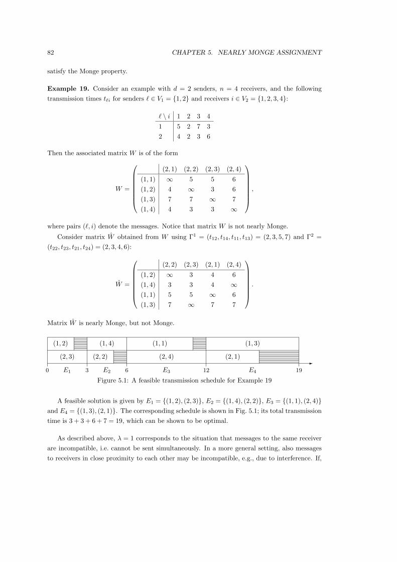
82 CHAPTER 5. NEARLY MONGE ASSIGNMENT
satisfy the Monge property.
Example 19. Consider an example with d = 2 senders, n = 4 receivers, and the following
transmission times t`i for senders ` ∈ V1 = 1, 2 and receivers i ∈ V2 = 1, 2, 3, 4:
` \ i 1 2 3 4
1 5 2 7 3
2 4 2 3 6
Then the associated matrix W is of the form
W =
(2, 1) (2, 2) (2, 3) (2, 4)
(1, 1) ∞ 5 5 6
(1, 2) 4 ∞ 3 6
(1, 3) 7 7 ∞ 7
(1, 4) 4 3 3 ∞
,
where pairs (`, i) denote the messages. Notice that matrix W is not nearly Monge.
Consider matrix W obtained from W using Γ1 = (t12, t14, t11, t13) = (2, 3, 5, 7) and Γ2 =
(t22, t23, t21, t24) = (2, 3, 4, 6):
W =
(2, 2) (2, 3) (2, 1) (2, 4)
(1, 2) ∞ 3 4 6
(1, 4) 3 3 4 ∞(1, 1) 5 5 ∞ 6
(1, 3) 7 ∞ 7 7
.
Matrix W is nearly Monge, but not Monge.
-
(1, 2)
(2, 3)
(1, 4)
(2, 2)
(1, 1)
(2, 4)
(1, 3)
(2, 1)
E1 E2 E3 E40 3 6 12 19
Figure 5.1: A feasible transmission schedule for Example 19
A feasible solution is given by E1 = (1, 2), (2, 3), E2 = (1, 4), (2, 2), E3 = (1, 1), (2, 4)and E4 = (1, 3), (2, 1). The corresponding schedule is shown in Fig. 5.1; its total transmission
time is 3 + 3 + 6 + 7 = 19, which can be shown to be optimal.
As described above, λ = 1 corresponds to the situation that messages to the same receiver
are incompatible, i.e. cannot be sent simultaneously. In a more general setting, also messages
to receivers in close proximity to each other may be incompatible, e.g., due to interference. If,

5.3. NP-HARDNESS OF PROBLEM AP(D,λ) 83
for example, for each receiver one or two ‘neighbors’ are affected, we get problems with λ = 2
or λ = 3.
Example 19 can be reformulated to define an instance of the synchronous open shop problem,
replacing “senders” and “receivers” by “machines” and “jobs”, respectively. The entries of
matrices W and W remain the same. In the schedule shown in Fig. 5.1, the sets E1, E2, E3 and
E4 have now the meaning of cycles, while pairs (`, i) represent now operations O`i. Note that
this example uses the same set of jobs as Example 2 in Section 4.1, although the numbering of
the jobs is different (recall that in Section 4.1 jobs were numbered by non-increasing processing
times on the first machine).
In the subsequent sections we will also consider the relaxed versions of both synchronous
open shop scheduling and satellite communication, where some senders or machines are allowed
to stay idle so that less than d activities may occur in a cycle or period. As we already
demonstrated for two-machine synchronous open shop, there are instances for which an optimal
solution with idle times may outperform any solution without idle times. In the next section
we provide a construction, which helps modelling those versions as problem AP(d, λ), using a
concept similar to the idea of dummy jobs.
5.3 NP-hardness of problem AP(d, λ)
In this section we prove that problem AP(d, λ) with arbitrary d and fixed λ is strongly NP-hard,
even for λ = 1, via a reduction from max-weight edge coloring in complete bipartite graphs.
Recall that both applications described in Section 5.2 can be modelled as problem MEC on
complete bipartite graphs. Furthermore, we discuss the complementary result that AP(d, λ)
with arbitrary λ and fixed d is strongly NP-hard, even if d = 3.
While the NP-hardness of problem AP(d, λ) with arbitrary d and λ = 1 is not surprising, as
in the previous section we used it to model two problems known to be strongly NP-hard, there
is still value in providing a full, formal reduction. Firstly, using the same construction as in
the reduction below will later allow us to model the relaxed versions of both applications from
the previous section as problem AP(d, λ). Secondly, the construction provides a general way to
model any application of MEC on bipartite graphs, or of MVC on the line graphs of bipartite
graphs as problem AP(d, λ), instead of treating each application separate.
Theorem 20. Problem MEC(Km,n) reduces to problem AP(d, λ) with d = m and λ = 1,
MEC(Km,n) ∝ AP(m, 1). (5.6)
Proof: Without loss of generality we assume that m ≤ n. Clearly, the number of colors κ in
any feasible solution to MEC(Km,n) satisfies n ≤ κ ≤ nm, and the number of edges that get
the same color c ∈ 1, . . . , κ may vary from 1 to m.
We present the proof for m = 2 first and then generalize it for an arbitrary m. In order to

84 CHAPTER 5. NEARLY MONGE ASSIGNMENT
prove (5.6) for m = 2, we create an auxiliary problem MEC2n(K2,2n) which corresponds to the
MEC for the bipartite graph K2,2n with exactly 2n colors allowed. We show that
MEC(K2,n) ∝ MEC2n(K2,2n) (5.7)
and
MEC2n(K2,2n) ∝ AP(2, 1). (5.8)
Given a bipartite graph G = (V1 ∪ V2, E) for the original problem MEC(K2,n), create the
extended bipartite graph G = (V1 ∪ V2, E) for the auxiliary problem with unchanged first set
of vertices V1, while the second set of vertices V2 is extended by adding n additional vertices
so that |V2| = 2n. The edge set E is extended accordingly, to include mn = 2n new edges
connecting all vertices from V1 with the n auxiliary vertices from V2, the weights of those edges
being set to 0. Clearly, any feasible solution to MEC(K2,n) that uses κ colors can be extended
to a feasible solution to MEC2n(K2,2n) that uses 2n colors without changing the objective
value such that κ colors contribute to the weight function, while 2n− κ colors carry 0-weight.
Conversely, if we have a solution to MEC2n(K2,2n), we simply drop all auxiliary edges (having
weight 0) and obtain a feasible solution with the same objective value for MEC(K2,n). Thus,
reduction (5.7) holds.
In what follows we reformulate problem MEC2n(K2,2n) as an assignment problem which
finds for every edge (1, vi) a mate (2, vj) with 1, 2 ⊆ V1 and vi, vj ⊆ V2, such that both
edges can get the same color. Such a pair of edges in the same color contributes the amount
max w (1, vi) , w (2, vj) to the objective function.
First create two sequences of edges((
1, v11
),(1, v2
1
), . . . ,
(1, v2n
1
))and
((2, v1
2
),(2, v2
2
), . . . ,(
2, v2n2
))each consisting of 2n edges listed in non-decreasing order of their weights:
w(1, v1
1
)= w
(1, v2
1
)= · · · = w (1, vn1 ) ≤ w
(1, vn+1
1
)≤ · · · ≤ w
(1, v2n
1
),
w(2, v1
2
)= w
(2, v2
2
)= · · · = w (2, vn2 ) ≤ w
(2, vn+1
2
)≤ · · · ≤ w
(2, v2n
2
).
Here the first n terms of each list correspond to the edges incident to auxiliary vertices which
have 0-weights. We define the matrix W with 2n rows and 2n columns as follows:
– each row i, 1 ≤ i ≤ 2n, corresponds to the edge ei1 = (1, vi1);
– each column j, 1 ≤ j ≤ 2n, corresponds to the edge ej2 = (2, vj2);
– the weight-value wij corresponds to the weight of assigning the same color to the pair of
edges ei1 and ej2,
wij =
maxw(ei1), w(ej2), if vi1 6= vj2,
∞, otherwise.(5.9)
The matrix with entries maxw(ei1), w(ej2) is the two-dimensional case of (5.2) and therefore
satisfies the Monge property. Thus, matrix W defined by (5.9), where ∞-entries correspond to

5.3. NP-HARDNESS OF PROBLEM AP(D,λ) 85
incompatible pairs of edges ei1, ej2, is a nearly Monge matrix with λ = 1 incompatible partner
for every i = i∗ or j = j∗.
It is easy to see that for any feasible solution to problem MEC2n(K2,2n) there exists a feasible
solution to problem AP(2, 1) with the same (finite) weight and vice versa. Thus, reduction (5.8)
holds.
Consider now the case of an arbitrary m ≤ n. Given problem MEC(Km,n), introduce the
extended problem MECmn(Km,mn) by adding (m−1)n auxiliary vertices to V2 and introducing
edges of weight 0 that connect them with m vertices from V1. As before, any feasible solution
to MEC(Km,n) with κ colors can be extended to a feasible solution of MECmn(Km,mn) with
mn colors (and vice versa) such that κ colors contribute to the weight function, while mn− κcolors carry 0-weight. Thus,
MEC(Km,n) ∝ MECmn(Km,mn). (5.10)
In order to reduce MECmn(Km,mn) to AP(m, 1), create m sequences of edges
((h, v1
h
),(h, v2
h
), . . . , (h, vmnh )
),
each listed in non-decreasing order of the weights, 1 ≤ h ≤ m. The array W is m-dimensional,
with each dimension h corresponding to edges eih =(h, vih
)incident to h, the number of entries
in each dimension being mn. The weight-value wi1...im corresponds to the weight of assigning
the same color to m edges ei11 = (1, vi11 ), ei22 = (2, vi22 ), . . . , eimm = (m, vimm ),
wi1...im =
max1≤h≤m
w(eihh ), if all vertices vi11 , vi22 , . . . , v
imm are different,
∞, otherwise.(5.11)
Again, the array with entries max1≤h≤m
w(eihh ) satisfies the Monge property, see (5.2). There-
fore, the array W defined by (5.11), where∞-entries correspond to incompatible pairs of edges,
is a nearly Monge array with λ = 1 incompatible partner for every ih = i∗h. Thus, similar to
the two-dimensional case, we have
MECmn(Km,mn) ∝ AP(m, 1), (5.12)
which together with (5.10) proves the theorem.
In the proof of Theorem 20 we have developed reduction (5.7), which is useful for handling
the generalized versions of the two applications, scheduling satellite transmissions and syn-
chronous open shop problems. These two problems were introduced in Section 5.2 under the
assumption that exactly d activities should be assigned in each period/cycle. Both problems
were modelled as AP(d, 1) by defining for each sender or machine `, 1 ≤ ` ≤ d, the n-tuple
Γ` =(γ`1, γ
`2, . . . , γ
`n
), where γ-values are in the non-decreasing order (5.4), and by setting up

86 CHAPTER 5. NEARLY MONGE ASSIGNMENT
the cost array W of the form:
wi1...id =
max
γ1i1, γ2i2, . . . , γdid
, if all activities corresponding to γ1
i1, . . . , γdid
are compatible,
∞, otherwise,
(5.13)
see (5.5) and (5.3). If fewer than d activities per period/cycle are allowed, then using the same
idea as in reduction (5.10) together with (5.12), the two applications are modelled as AP(d, 1)
with n actual receivers/jobs and (d− 1)n auxiliary ones. We set the γ-values for the auxiliary
receivers/jobs to 0. Then each extended dn-tuple Γ` is of the form
Γ` =
0, 0, . . . , 0︸ ︷︷ ︸d(n−1) elements
, γ`1, γ`2, . . . , γ
`n︸ ︷︷ ︸
n elements
.
This results in the extended cost array W with entries of type (5.13) defined for dn receivers/jobs
rather than for n. If parameters d and λ are fixed, then the O(n)-time algorithm of Section 5.6
solves the associated applied problems in linear time, after sorting the input data in order to
achieve (5.4).
We now turn to complexity aspects of problem AP(d, λ) with one parameter fixed and
another one being part of the input. If λ = 0, then the weight array of problem AP(d, 0) is
Monge rather than nearly Monge, and an optimal solution is of the diagonal structure [26]. For
the case of λ = 1 we use Theorem 20 and the NP-hardness result known for MEC(Km,n) from
[43, 126] to make the following conclusion.
Observation 21. Problem AP(d, 1), where d ≥ 2 is part of the input, is NP-hard in the strong
sense, even if there are only three distinct finite weights.
Note that the restriction related to three weight values, except for ∞’s, follows from the
reduction presented in [126], which uses only three distinct weights. Interestingly, problem
MEC(Kn,n) with two distinct weights is solvable in polynomial time, as shown in [43, 126].
Consider now the counterpart of AP(d, λ) with fixed d and an arbitrary λ. If d = 2, then
problem AP(2, λ) can be solved in O(n3) time by the Hungarian algorithm [25, 88] that finds
an optimal solution to the assignment problem with an arbitrary, not necessarily Monge-like
matrix. If d = 3, then problem AP(3, λ) becomes NP-hard in the strong sense.
Observation 22. If λ is part of the input, then problem AP(3, λ) is NP-hard in the strong
sense, even if all finite weights are equal.
To justify Observation 22 we establish a link between problem AP(3, λ) and the famous 3-
DIMENSIONAL MATCHING problem (3-DM) known to be strongly NP-complete [59]. Recall
that in 3-DM, there are given three disjoint sets X, Y and Z, with n elements in each, and
a set of triples M ⊆ (X × Y × Z); the goal is to find a perfect matching, i.e. a set M ′ ⊆ M ,
5.4. PROPERTIES OF NEARLY MONGE MATRICES 87
such that each element from X, Y and Z appears in exactly one triple in M ′, see [59]. Any
instance of problem AP(3, λ) with all finite weights equal to 0 can be treated as an instance
of problem 3-DM, where the set M consists of all triples excluding those with incompatible
partner indices. We denote this special case of 3-DM by 3-DM(λ). Conversely, any instance of
problem 3-DM(λ) can be treated as an instance of problem AP(3, λ) where all finite weights
are 0. Clearly, there exists a perfect matching for an instance of 3-DM(λ) if and only if there
exists an assignment of cost 0 for the corresponding instance of AP(3, λ). Thus,
3-DM(λ) ∝ AP(3, λ).
In order to demonstrate the NP-completeness of 3-DM(λ), consider the well-known NP-
completeness proof for 3-DM. It is based on the reduction 3-SAT∝ 3-DM presented, e.g., in
[59]. Without changing the structure of the instance of 3-DM used in the proof, one can re-
define it as an instance of 3-DM(λ) with λ = n − 1, so that the reduction from [59] becomes
3-SAT∝ 3-DM(λ). So as to not distract from the core problem of this chapter we do not provide
such a re-definition at this point. For an interested reader, it is instead provided in Section 5.8
at the end of this chapter. All in all, we get the chain of reductions
3-SAT ∝ 3-DM(λ) ∝ AP(3, λ),
which proves Observation 22.
The complexity results discussed in this section are summarized in Table 7.2 in the Conclu-
sions.
5.4 Some properties of nearly Monge matrices with in-
compatible partner indices
In this and in the subsequent sections we consider problem AP(d, λ) with fixed d and λ. Prior
to discussing algorithmic aspects, we first demonstrate in Section 5.4.1 that the existing results
known for the assignment problem with∞’s are generally inapplicable. Then in Sections 5.4.2-
5.4.3 we address several typical questions that arise in the context of matrices with∞’s or with
unspecified entries.
5.4.1 Nonexistence of a Monge sequence
As explained before, the introduction of∞-entries into a Monge matrix may destroy the Monge
property. In the literature on Monge-like structures it is then suggested to verify whether a
non-Monge matrix possesses a so-called Monge sequence. Such a sequence guides a greedy
algorithm towards finding an optimal solution to the assignment or transportation problem
[26, 74]. It considers the variables in the order they appear in a Monge sequence and assigns

88 CHAPTER 5. NEARLY MONGE ASSIGNMENT
the highest possible values to them without violating the constraints of the problem. Formally,
a Monge sequence of an n × n matrix W = (wij) is defined as a sequence of n2 index pairs
(i1, j1), . . . , (in2 , jn2) such that whenever (i, j) precedes both (i, s) and (r, j) in the sequence,
condition
wij + wrs ≤ wis + wrj (5.14)
holds (cf. [74]).
A Monge sequence, if one exists, is a powerful tool for solving problems with matrices which
do not satisfy the Monge property for all quadruples. Models of this type arise for example
in the scheduling context. The scheduling problems studied in [72, 73] can be modelled as
transportation problems with non-Monge matrices. In some cases Monge sequences can be
found efficiently; in others a Monge sequence does not exist, and this calls for a development
of special tailor-made algorithms, as in the case of the generalized (weighted) version of the
problem from [73].
Even for the simplest version of our problem AP(d, λ) with d = 2 and λ = 1 the matrices in
general do not possess a Monge sequence. Consider the two applications discussed in Section 5.2
with a cost matrix of type (5.2). If the w-values are defined as
wij =
maxi, j, if i 6= j,
∞, otherwise,
and the matrix is at least of size 3×3, then a Monge sequence does not exist. Indeed, whichever
element is selected as the first element of a Monge sequence, the sequence cannot be completed
to satisfy (5.14). For any selected entry there always exists an ∞-entry that is not in the same
row and not in the same column, while the other two entries of the associated quadruple are
finite. Clearly, condition (5.14) is violated for such a quadruple. For a more general case, a
similar example can be found in [138], where finite entries of W are arbitrary.
Observation 23. In general, nearly Monge arrays with incompatible partners do not give rise
to Monge sequences even for λ = 1 and d = 2.
5.4.2 Recognizing nearly Monge arrays
Given a weight matrix W , it is easy to verify whether the Monge property (2.3) is satisfied for
finite entries. A straight-forward way to do so is to check (2.3) for all pairs of finite entries
of the form (wij , wrs) with i < r and j < s, which takes no more than O(n4) checks. This
method can also be generalized to recognize d-dimensional nearly Monge arrays, in which case
it takes no more than O(n2d) checks. Note that a d-dimensional nearly Monge array consists
of nd entries.
The applications discussed in Section 5.2 and the MEC problem of Section 5.3 deal with
a weight array W of form (5.2) with ∞-entries introduced for incompatible partners. Even if
initially W is not nearly Monge, that property can be achieved by ordering the γ-values of lists

5.4. PROPERTIES OF NEARLY MONGE MATRICES 89
Γ`, which is equivalent to sequencing the sets I and J of the assignment problem, or permuting
the rows and columns of W . In general, however, recognizing a permuted nearly Monge array
is a non-trivial task, as discussed below. Array W is a permuted nearly Monge array if its index
sets can be permuted to make the array nearly Monge.
Observation 24. For an arbitrary λ, it is NP-complete to decide whether a given array with
at most λ incompatible partners (for every index) is permuted nearly Monge, even for d = 2
(i.e. the matrix case).
This observation follows from a similar result in [41] formulated for a permuted incomplete
Monge matrix, which is equivalent to a nearly Monge matrix with an arbitrary λ. Notice that
recognizing a permuted Monge matrix can be done in O(n2) time [26], and recognizing a special
incomplete Monge matrix, namely a Supnick matrix, which is a symmetric Monge matrix with
unspecified diagonal entries, can be done in O(n2 log n) time [41].
In the nearly Monge case, if the number of incompatible partners λ is fixed, recognition
of permuted nearly Monge matrices remains open. If a polynomial-time algorithm could be
developed, it would be beneficial to achieve a time complexity smaller than O(n3), beating the
time complexity of solving a general assignment problem.
Further difficulties arise in recognition of nearly Monge arrays for higher dimensions d ≥ 3.
It is known that in the absence of ∞’s, a d-dimensional array W is a Monge array if and
only if every two-dimensional submatrix is a Monge matrix [2]. This property can then be
efficiently used in recognizing d-dimensional Monge arrays [130]. Unfortunately this necessary
and sufficient condition no longer holds for nearly Monge arrays, even if λ = 1. Consider
for example a three-dimensional array W = (wijk) with n = 3, λ = 1, incompatible partners
(1, 2, ∗), (2, 1, ∗), (1, ∗, 3), (2, ∗, 2), (3, ∗, 1), (∗, 1, 2), (∗, 2, 3), two 1-entries w111 = w333 = 1 and
all remaining finite entries being 0’s. The two-dimensional submatrices are listed below, and all
of them are nearly Monge. However, because of w111 + w333 = 2 > 0 = w131 + w313, the array
W is not a nearly Monge array.
i = 1 : i = 2 : i = 3 : 1 ∞ ∞∞ ∞ ∞0 0 ∞
∞ ∞ ∞
0 ∞ ∞0 ∞ 0
∞ ∞ 0
∞ 0 ∞∞ 0 1
j = 1 : j = 2 : j = 3 : 1 ∞ ∞
∞ ∞ ∞∞ ∞ 0
∞ ∞ ∞
0 ∞ ∞∞ 0 ∞
0 0 ∞
0 ∞ 0
∞ 0 1

90 CHAPTER 5. NEARLY MONGE ASSIGNMENT
k = 1 : k = 2 : k = 3 : 1 ∞ 0
∞ 0 0
∞ ∞ ∞
∞ ∞ 0
∞ ∞ ∞∞ 0 0
∞ ∞ ∞∞ ∞ 0
0 ∞ 1
Observation 25. Even if every two-dimensional submatrix of a d-dimensional array W with
λ = 1 is a nearly Monge matrix, the whole array W is not necessarily a nearly Monge array.
5.4.3 Completing nearly Monge arrays
An interesting question related to arrays with unspecified or∞-entries is the possibility of com-
pleting them by introducing finite values in order to achieve Monge arrays. Such an approach
works, for example, for incomplete matrices of Supnick type, as shown in [41], but unfortunately,
it does not work for nearly Monge matrices. Consider the following nearly Monge matrix with
λ = 1: 0 0 1 ∞ 0
1 0 0 0 ∞4 2 ∞ 0 1
6 ∞ 2 0 0
∞ 6 4 1 0
.
Attempting to complete that matrix without permuting rows and columns, we have to satisfy
the following two contradicting conditions for w14:
w14 + w23 ≥ w13 + w24, or equivalently w14 ≥ 1,
w14 + w35 ≤ w15 + w34, or equivalently w14 ≤ −1.
Attempting to permute and complete the above matrix, the only suitable permutation of rows
and columns that preserves the Monge property for finite entries is the one which reverses the
orders of rows and columns (notice that all quadruples with finite entries satisfy the Monge
property as strict inequalities). The arguments for entry w14 can be re-used with respect to the
entry w52 in the permuted matrix, justifying that completing cannot be done.
Observation 26. In general, a nearly Monge matrix with incompatible partners cannot be
completed into a Monge matrix by replacing ∞-entries by finite values even for λ = 1.
If permutations of rows and columns are fixed, producing a completed Monge matrix, if one
exists, can be done in polynomial time by solving the following system of linear inequalities:
wij + wi+1,j+1 ≤ wi,j+1 + wi+1,j , 1 ≤ i, j < n,
wij = wij , 1 ≤ i, j < n, wij 6=∞,wij ∈ R.
Here wij are real-valued variables representing the target values of wij . Notice that for a Monge

5.5. THE CORRIDOR PROPERTY FOR PROBLEM AP(D,λ) 91
matrix it is sufficient to achieve the Monge property for quadruples defined by adjacent pairs
of rows and columns [26].
If a feasible solution satisfying the above inequalities exists, real values are assigned to all∞-
entries, so that the resulting Monge matrix W is a completion of W . In the case of infeasibility,
either the matrix W is not nearly Monge (i.e. not all quadruples of finite entries satisfy the
Monge property) or the matrix W is not completable to a Monge matrix.
Notice that in the applications, which arise in scheduling satellite transmissions or syn-
chronous open shops, nearly Monge arrays are completable if the formulae for w’s (5.5) and
(5.3) are modified accordingly, namely, by assigning finite values maxγ1i1, γ2i2, . . . , γdid
to all
d-tuples (i1, i2, . . . , in), ignoring the condition that all receivers or all jobs should be different.
Also, formula (3.1) for MEC (Km,n) can be adjusted to replace∞’s by values maxw(e)|e ∈ Ecfor any combinations of m edges with different origins in V1, even if there are repeated vertices
in V2. Due to the sorting and the max-definition (5.2), the resulting array is Monge.
5.5 The corridor property for problem AP(d, λ)
In this section we consider the assignment problem AP(d, λ) with a d-dimensional nearly Monge
weight array W and at most λ incompatible partners for every index. We show that there exists
an optimal solution S such that all non-zero entries xi1,...,id = 1 of the solution matrix XS lie
in a corridor of a certain width ξ around the main diagonal,
|i` − i1| ≤ ξ for all ` = 1, . . . , d, (5.15)
where
ξ = d(d− 1)λ. (5.16)
We refer to the above condition as the corridor property. Based on it, in the next section we
develop a linear-time algorithm to solve problem AP(d, λ) for fixed d and λ. Note that AP(d, λ)
is strongly NP-hard, if d or λ is part of the input, see Section 5.3.
Theorem 27. For problem AP(d, λ) there exists an optimal solution
S = (ı11, ı12, . . . , ı1d), (ı21, ı22, . . . , ı2d), . . . , (ın1 , ın2 , . . . , ınd )
such that every d-tuple (i1, i2, . . . , id) = (ık1 , ık2 , . . . , ı
kd), 1 ≤ k ≤ n, satisfies (5.15) with ξ defined
by (5.16).
Proof: Starting with an optimal solution S =
(i11, i12, . . . , i
1d), . . . , (i
n1 , i
n2 . . . , i
nd )
that violates
the corridor property (5.15) we perform a series of exchange steps, each of which does not
increase the cost, eventually producing a solution that satisfies (5.15). We assume that w(S) <
∞, i.e., none of the d-tuples in S contains a pair of incompatible partners; otherwise S can be
replaced by the diagonal solution, which has the desired property and no higher cost.

92 CHAPTER 5. NEARLY MONGE ASSIGNMENT
For the exchange step, we take a d-tuple (i1, i2, . . . , id) of the current solution that violates
(5.15), select a special companion d-tuple (j1, j2, . . . , jd) from the current solution and replace
that pair by (s1, s2, . . . , sd) and (t1, t2, . . . , td) defined by
s` = min i`, j` , t` = max i`, j` , ` = 1, . . . , d. (5.17)
Since W is nearly Monge, the inequality
ws1s2...sd + wt1t2...td ≤ wi1i2...id + wj1j2...jd
holds, if none of the four entries is ∞. With an appropriate choice of the companion d-tuple
(j1, j2, . . . , jd), we eliminate the violation related to (i1, i2, . . . , id) without increasing the cost.
We distinguish between two types of violations:
Type I(i`) violation : i` > i1 + ξ for i1 ≤ n− ξ − 1,
Type II(i`) violation : i` < i1 − ξ for i1 ≥ ξ + 1,
and use the terms “d-tuple of Type I(i`)” and “d-tuple of Type II(i`)” for violating d-tuples.
First we eliminate Type I(i2) violations for the second index. We start with the d-tuple of
Type I(i2) with the smallest first index i1 and then we proceed with other d-tuples of Type I(i2)
considering them in increasing order of i1. After that we eliminate all Type II(i2) violations,
starting with the d-tuple of Type II(i2) with the largest first index i1, proceeding then with
other d-tuples of Type II(i2) considered in decreasing order of i1.
Having eliminated all Type I(i2) and Type II(i2) violations for the second index, we proceed
with violations for the third index. We handle them in the same order, fixing first Type I(i3)
violations with d-tuples of Type I(i3) considered in increasing order of i1, and then Type II(i3)
violations with d-tuples of Type II(i3) considered in decreasing order of i1. For these exchanges
we demonstrate that no new violations of Type I(i2) and Type II(i2) for second indices are
created. The same approach is then applied to the remaining indices i4, . . ., id.
Eliminating violations of Type I(i2). Among all d-tuples with violations of Type I(i2), select
the d-tuple(i1, i2, . . . , id
)with the smallest first index i1, so that
i2 > i1 + ξ . (5.18)
Note that the choice of i1 implies that no Type I(i2) violations happen for i1 < i1. For the
violating d-tuple(i1, i2, . . . , id
)select a companion d-tuple (j1, j2, . . . , jd) with
j1 > i1 and j2 ≤ i1 + ξ (5.19)
such that
(a) xj1j2...jd = 1 in the current solution (recall that the associated value of wj1j2...jd cannot be

5.5. THE CORRIDOR PROPERTY FOR PROBLEM AP(D,λ) 93
∞ then),
(b) the induced d-tuples (s1, s2, . . . , sd), (t1, t2, . . . , td) defined by (5.17) correspond to finite
entries in W , i.e. do not contain two incompatible partner indices.
Figure 5.2: Eliminating Type I(i2) violation(a) Solution matrix XS with the violating d-tuple (i1, i2, . . . , id) of Type I(i2)(b) Modified solution matrix X ′S with Type I(i2) violation in row i1 eliminated
For violation (5.18) the required d-tuple (j1, j2, . . . , jd) exists since, as we show below, there
are ξ + 1 candidate 1-entries with indices j1 and j2 satisfying (5.19). Clearly, at least one of
those ξ + 1 candidates has all indices compatible with the indices from(i1, i2, . . . , id
). If this
was not the case, i.e., if there was at least one incompatible index between(i1, i2, . . . , id
)and
each of the ξ + 1 candidate entries, then the total number of incompatible partner indices for(i1, i2, . . . , id
)would be equal to ξ + 1 = d(d− 1)λ+ 1, a contradiction to the assumption that
for any index iu = iu, 1 ≤ u ≤ d, there are at most Ω = λ (d− 1) incompatible partners, see
(5.1).
We now justify that there are indeed ξ+1 candidate 1-entries with indices j1 and j2 satisfying
(5.19). We start with the 2-dimensional case, with the binary solution matrix XS = (xi1i2)

94 CHAPTER 5. NEARLY MONGE ASSIGNMENT
illustrated in Fig. 5.2 (a). The symbol “×” in Fig. 5.2 is used to mark compulsory 0’s in the
solution matrix, caused by incompatible partner indices.
Consider the first (i1 + ξ) columns of the associated matrix XS , marked by a rounded
rectangle in Fig. 5.2 (a). Since every column of XS contains one 1-entry, the selected part
contains (i1 + ξ) 1-entries. By the assumption, there are no violations of Type I(i2) for the first
(i1 − 1) rows; therefore the first (i1 − 1) rows of the selected part contain (i1 − 1) 1-entries in
columns 1, 2, . . ., i1 + ξ − 1, and they do not contain 1-entries in column i1 + ξ. Thus, the
remaining part of the selection, corresponding to rows i1 +1, . . ., n and columns 1, 2, . . ., i1 +ξ,
contains (i1 + ξ
)−(i1 − 1
)= ξ + 1
1-entries.
It is easy to see that the same arguments are applicable for the multi-dimensional case.
Fig. 5.2 can be treated as a ‘projection’ of the d-dimensional case into the space of the first two
indices with
xi1i2 =∑
i3,...,id
xi1i2i3...id .
Replacing(i1, i2, . . . , id
), (j1, j2, . . . , jd) by (s1, s2, . . . , sd), (t1, t2, . . . , td) eliminates the cur-
rent Type I(i2) violation for i1 = i1. Note that it does not matter whether the companion
d-tuple (j1, j2, . . . , jd) is violating or not; that d-tuple is removed from the solution as a result
of the exchange step. It also does not matter whether (s1, s2, s3, . . . , sd) =(i1, j2, s3, . . . , sd
)or
(t1, t2, . . . , td) =(j1, i2, t3, . . . , td
)are violating: a possible violation for (s1, s2, . . . , sd) can only
be of Type II(i2), as s2 = j2 ≤ i1 + ξ by (5.19), and it is repaired at a later stage; a possible
violation for (t1, t2, . . . , td) may be of any type, but due to t1 = j1 > i1 it is also repaired at a
later stage.
Proceeding with each next smallest index i1, for which violation of Type I(i2) occurs, all
Type I(i2) violations are repaired in a similar way, resulting in a solution where no Type I(i2)
violations remain.
Eliminating violations of Type II(i2). Among all d-tuples with violations of Type II(i2),
select the d-tuple(i1, i2, i3, . . . , id
)with the largest first index i1, so that the corridor property
is satisfied for the second index for any i1 > i1 and the violation under consideration is of the
form
i2 < i1 − ξ , (5.20)
see Fig. 5.3. The required companion d-tuple (j1, j2, . . . , jd) should satisfy
j1 < i1 and i1 − ξ ≤ j2 ≤ i1 + ξ , (5.21)
together with properties (a)–(b) formulated for Type I(i2) violations.
For violation (5.20) the required d-tuple (j1, j2, . . . , jd) exists since, as we show below, there

5.5. THE CORRIDOR PROPERTY FOR PROBLEM AP(D,λ) 95
Figure 5.3: Eliminating Type II(i2) violation(a) Solution matrix XS with the violating d-tuple (i1, i2, . . . , id) of Type II(i2)(b) Modified solution matrix X ′S with Type II(i2) violation in row i1 eliminated
are ξ + 1 candidate 1-entries with indices j1 and j2 satisfying
j1 < i1 and i1 − ξ ≤ j2 ≤ i1 + ξ − 1, (5.22)
which is in fact a stronger condition than (5.21). Again, at least one of those ξ + 1 entries has
all indices compatible with the indices from(i1, i2, . . . , id
), so that the exchange step with the
induced d-tuples (s1, s2, . . . , sd), (t1, t2, . . . , td) achieves its goal.
To justify that there exist ξ + 1 candidate 1-entries with indices j1 and j2 satisfying (5.22),
consider first the 2-dimensional case. Since XS does not contain Type I(i2) violations, all

96 CHAPTER 5. NEARLY MONGE ASSIGNMENT
(i1 − 1
)1-entries of the
(i1 − 1
)first rows belong to the area marked by the larger rounded
rectangle in Fig. 5.3 (a) with j2 ≤ i1+ξ−1. Moreover, the part of the selected area j2 ≤ i1−ξ−1,
marked by the smaller rounded rectangle in Fig. 5.3 (a), contains no more than(i1 − ξ − 1
)1-entries. In fact it contains no more than
(i1 − ξ − 2
)1-entries since the 1-entry in column i2
does not belong to the selected area. Thus, the remaining part of the selection, corresponding
to rows 1, 2, . . . , i1 − 1 and columns i1 − ξ, . . . , i1 + ξ − 1 contains
(i1 − 1
)−(i1 − ξ − 2
)= ξ + 1
1-entries, which all satisfy (5.22). Again it is easy to see that the same arguments hold for the
d-dimensional case.
Replacing(i1, i2, . . . , id
), (j1, j2, . . . , jd) by (s1, s2, . . . , sd), (t1, t2, . . . , td) eliminates vio-
lation (5.20), so that the corridor property is now achieved for the second index for any
i1 ≥ i1. Note that (t1, t2, . . . , td) =(i1, j2, t3, . . . , td
)satisfies the corridor property, while
(s1, s2, s3, . . . , sd) =(j1, i2, s3, . . . , sd
)may violate it. The possible violation is of Type II(i2)
with s1 < i1, and it is repaired at a later stage.
Proceeding with each next largest index i1, for which a violation of Type II(i2) occurs, all
Type II(i2) violations are repaired in a similar way, resulting in a solution where no violations
of any type remain for the second index.
After all violations of Type I(i2) and Type II(i2) are eliminated, we start eliminating viola-
tions for the third index, ensuring that no new violations are created for the second index. We
use the same approach:
– first eliminate all violations of Type I(i3), starting with a violating d-tuple with the
smallest i1, and proceeding then with other violating d-tuples considered in increasing
order of i1;
– next eliminate all violations of Type II(i3), starting with a violating d-tuple with the
largest i1, and proceeding with other violating d-tuples considered in decreasing order of
i1.
The existence of the d-tuple (j1, j2, . . . , jd) needed for the exchange step can be proven in the
same way as above. We only need to demonstrate that the induced d-tuples (s1, s2, . . . , sd),
(t1, t2, . . . , td), defined in accordance with (5.17), do not create new violations in the previously
repaired second index, while repairing violations in the third one.
Consider the exchange step based on (i1, i2, . . . , id) and (j1, j2, . . . , jd) with
i1 < j1. (5.23)

5.6. A LINEAR-TIME ALGORITHM 97
Since in this stage violations for the second index have been already repaired, we have
−ξ ≤ i2 − i1 ≤ ξ , (5.24)
−ξ ≤ j2 − j1 ≤ ξ . (5.25)
If i2 < j2, then the induced d-tuples are of the form (i1, i2, s3. . . , sd), (j1, j2, t3. . . , td), and by
(5.24)-(5.25) no new violation appears for the second index. Alternatively, if
i2 > j2, (5.26)
then for the induced d-tuple (i1, j2, s3. . . , sd) there is no violation for the second index since
j2 − i1 > −ξ by (5.23) and by the first inequality from (5.25),
j2 − i1 < ξ by (5.26) and by the second inequality from (5.24).
For the induced d-tuple (j1, i2, s3. . . , sd) there is also no violation for the second index since
i2 − j1 > −ξ by (5.26) and by the first inequality from (5.25),
i2 − j1 < ξ by (5.23) and by the second inequality from (5.24).
It is easy to verify that if instead of (5.23) condition i1 > j1 holds, then similar arguments
are applicable. Thus, repairing violations related to the third index in the described way cannot
create violations related to the second one.
Using the same approach repeatedly, we eliminate violations with respect to each index i`,
` = 4, . . . , d. Each time, when eliminating violations for i`, we do not create new violations for
indices i2, i3, . . . , i`−1. This completes the proof of Theorem 27.
5.6 A linear-time algorithm for problem AP(d, λ) with fixed
d and λ
In this section we consider problem AP(d, λ) with fixed d and λ and develop a linear-time
algorithm for it. We start with the two-dimensional problem AP(2, λ).
By Theorem 27, we can restrict the search to solutions S such that all 1-entries appear inside
the corridor, which can be considered as a combination of the main diagonal, 2λ diagonals above
it and 2λ diagonals below it. An example of a solution matrix XS that satisfies the described
property is presented below for λ = 1, d = 2 and n = 10, with the corridor for 1-entries marked
by ∗:

98 CHAPTER 5. NEARLY MONGE ASSIGNMENT
XS 1 2 3 4 5 6 7 8 9 10
1 * * * 0 0 0 0 0 0 0
2 * * * * 0 0 0 0 0 0
3 * * * * * 0 0 0 0 0
4 0 * * * * * 0 0 0 0
5 0 0 * * * * * 0 0 0
6 0 0 0 * * * * * 0 0
7 0 0 0 0 * * * * * 0
8 0 0 0 0 0 * * * * *
9 0 0 0 0 0 0 * * * *
10 0 0 0 0 0 0 0 * * *
Introduce a layered network L = (s, t, V,A) with the vertex set V consisting of disjoint
subsets V (0), V (1), . . . , V (n), V (n+ 1). Subsets V (0) and V (n+ 1) are single-element
subsets containing the source V (0) = s and the sink V (n+ 1) = t. The arcs A have end
vertices belonging to two consecutive layers, A =⋃nk=0 (V (k)× V (k + 1)). The vertices of
layer V (k), 1 ≤ k ≤ n, characterize the partial solutions consisting of the first k rows and
satisfying the corridor property.
For two vertices v`(k) ∈ V (k) and vm (k + 1) ∈ V (k + 1), let X`(k) and Xm (k + 1) be two
associated partial solutions. If X`(k) ⊂ Xm (k + 1), then the arc (v`(k), vm (k + 1)) has the
cost of assigning the 1-entry to a relevant position in row k + 1; that cost is given by wk+1,j ,
where j is the column with xk+1,j = 1 in Xm (k + 1). Otherwise v`(k) and vm (k + 1) are not
connected by an arc. For completeness, introduce auxiliary arcs of cost 0 from every vertex of
V (n) to t. Clearly, an optimal solution corresponds to a shortest path in the network L.
In order to reduce the size of L, we include in V (k) only the vertices corresponding to
non-dominated partial solutions: if X`′(k) and X`′′(k) have 1-entries assigned to the same set
of columns and w (X`′(k)) ≤ w (X`′′(k)), where w(X) represents the cost of the associated
solution, then it is sufficient to include in V (k) only one vertex corresponding to X`′(k). This
implies that each vertex of V (k) is characterized by a unique subset of columns which contain
1-entries in the first k rows. In order to estimate |V (k)|, we prove the following statement.
Statement 28. Any partial solution X`(k) of layer k consists of
(a) α columns 1, 2, . . . , α, each containing one 1-entry, where
α = max k − 2λ, 0 ,
(b) n− β columns β + 1, . . . , n, each containing 0-entries only, where
β = min k + 2λ, n ,
(c) among the columns α + 1, . . . , β there are (k − α) = min 2λ, k columns, each containing

5.6. A LINEAR-TIME ALGORITHM 99
one 1-entry, and (β − k) = min 2λ, n− k columns with 0-entries only.
The following example with k = 6, n = 10, λ = 1 illustrates the structure of a partial
solution X`(k):
(k − α) columns
α columns with 1-entries
with 1-entry (β − k) columns
each without 1-entries no 1-entries︷ ︸︸ ︷ ︷ ︸︸ ︷ ︷ ︸︸ ︷α↓
α+1↓
k↓
β↓
β+1↓
n↓
X`(k) 1 2 3 4 5 6 7 8 9 10
1 * * * 0 0 0 0 0 0 0
2 * * * * 0 0 0 0 0 0
3 * * * * * 0 0 0 0 0
4 0 * * * * * 0 0 0 0
5 0 0 * * * * * 0 0 0
k → 6 0 0 0 * * * * * 0 0
k + 1→ 7 0 0 0 0 * * * * * 0
Proof: Conditions (a) and (b) hold since by the corridor property there can be no 1-entry for
any combination of i ∈ k + 1, . . . , n and j ∈ 1, 2, . . . , α, and also for any combination of
i ∈ 1, 2, . . . , k and j ∈ β + 1, . . . , n.Condition (c) deals with the remaining entries of X`(k), in rows i ∈ 1, 2, . . . , k and columns
j ∈ α+ 1, . . . , β. By the definition of the assignment problem, the total number of 1-entries
in the first k rows and n columns is k, α of which appear in columns j ∈ 1, 2, . . . , α. Since
no 1-entry can appear in columns j ∈ β + 1, . . . , n, the number of the remaining 1-entries is
k − α.
Statement 28 implies that the number of different subsets of columns which may contain
1-entries, and equivalently |V (k)|, depends on the selection of (k − α) columns out of (β − α)
columns in the middle part of the solution matrix. Since k − α ≤ 2λ and β − α ≤ 4λ, |V (k)|can be bounded by
θ =
(4λ
2λ
). (5.27)
Thus, the described approach reduces the assignment problem AP(2, λ) to the shortest path
problem in the layered network L, where the number of layers is n+2 and in each layer there are
no more than θ vertices. The network can be constructed inO (|A|) time, where |A| ≤ θ2 (n+ 1).
An optimal solution can be found by dynamic programming in O (|A|) = O(n) time as well.
Consider now the d-dimensional problem AP(d, λ) for fixed d ≥ 2 and fixed λ. Statement 28

100 CHAPTER 5. NEARLY MONGE ASSIGNMENT
can be generalized by replacing 2λ by ξ = d(d− 1)λ, so that
α = max k − ξ, 0 ,β = min k + ξ, n ,
k − α = min ξ, k ,β − k = min ξ, n− k .
Any feasible d-dimensional partial solution X`(k) consists of k 1-entries with i1 ∈ 1, 2, . . . , k.For each index iz, 2 ≤ z ≤ d, α of these 1-entries have iz ∈ 1, 2, . . . , α, 2 ≤ z ≤ d, and the
remaining (k − α) 1-entries have iz ∈ α+ 1, . . . , β. Due to this, the number of nodes |V (k)|in layer k depends on the selection of (k − α) choices for each index iz, 2 ≤ z ≤ d, out of (β − α)
possible choices. Since k − α ≤ ξ and β − α ≤ 2ξ, |V (k)| can be bounded by Θd−1, where Θ is
the amount of possible combinations for one fixed index iz,
Θ =
(2ξ
ξ
). (5.28)
There are at most Θ2(d−1) arcs in-between two layers, if each vertex in one layer is con-
nected to every vertex in the next one. Therefore the total number of arcs |A| is bounded
by Θ2(d−1) (n+ 1), and this defines the time complexity of solving the associated shortest path
problem by dynamic programming. Observe that a tighter estimate for |A| can be derived with
a more careful analysis of the arc set.
The complexity estimate Θ2(d−1) (n+ 1) with Θ defined by (5.28) implies that problem
AP(d, λ) is solvable in O(n) time if d and λ are fixed, and it is fixed-parameter tractable
(FPT), with parameters d and λ.
Going back to the applications discussed in Sections 5.2-5.3 we observe that they correspond
to the case of d = m and λ = 1, so that the described approach implies theO(n) time complexity.
Since modelling the two applications as AP(d, 1) incurs sorting the input data in non-decreasing
order and extending the instance (as described in Section 5.3 after the proof of Theorem 20),
we obtain the following corollary.
Corollary 29. The problems of scheduling satellite transmissions or synchronous open shops
and problem MEC(Km,n) with m = d are solvable in O(n log n) time if d is fixed, and they are
fixed parameter tractable if d is a parameter.
We conclude this section by analyzing the maximization version of problem AP(d, λ). In
that problem incompatible partners should be modelled by −∞-entries in the weight array W ,
in order to discourage their choice. In the following, we use the notion of an inverse Monge
array W : such an array satisfies the Monge property (2.4) with “≤” replaced by “≥” [26].
Equivalently, array W is inverse Monge if and only if −W is Monge.
The maximization version of problem AP(d, λ) is
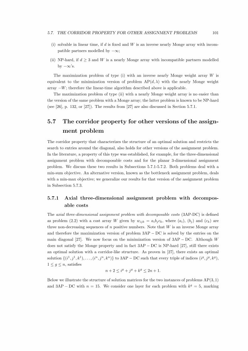
5.7. THE CORRIDOR PROPERTY FOR OTHER ASSIGNMENT PROBLEMS 101
(i) solvable in linear time, if d is fixed and W is an inverse nearly Monge array with incom-
patible partners modelled by −∞;
(ii) NP-hard, if d ≥ 3 and W is a nearly Monge array with incompatible partners modelled
by −∞’s.
The maximization problem of type (i) with an inverse nearly Monge weight array W is
equivalent to the minimization version of problem AP(d, λ) with the nearly Monge weight
array −W ; therefore the linear-time algorithm described above is applicable.
The maximization problem of type (ii) with a nearly Monge weight array is no easier than
the version of the same problem with a Monge array; the latter problem is known to be NP-hard
(see [26], p. 132, or [27]). The results from [27] are also discussed in Section 5.7.1.
5.7 The corridor property for other versions of the assign-
ment problem
The corridor property that characterizes the structure of an optimal solution and restricts the
search to entries around the diagonal, also holds for other versions of the assignment problem.
In the literature, a property of this type was established, for example, for the three-dimensional
assignment problem with decomposable costs and for the planar 3-dimensional assignment
problem. We discuss these two results in Subsections 5.7.1-5.7.2. Both problems deal with a
min-sum objective. An alternative version, known as the bottleneck assignment problem, deals
with a min-max objective; we generalize our results for that version of the assignment problem
in Subsection 5.7.3.
5.7.1 Axial three-dimensional assignment problem with decompos-
able costs
The axial three-dimensional assignment problem with decomposable costs (3AP-DC) is defined
as problem (2.2) with a cost array W given by wijk = aibjck, where (ai), (bj) and (ck) are
three non-decreasing sequences of n positive numbers. Note that W is an inverse Monge array
and therefore the maximization version of problem 3AP−DC is solved by the entries on the
main diagonal [27]. We now focus on the minimization version of 3AP−DC. Although W
does not satisfy the Monge property and in fact 3AP−DC is NP-hard [27], still there exists
an optimal solution with a corridor-like structure. As proven in [27], there exists an optimal
solution (i1, j1, k1), . . . , (in, jn, kn) to 3AP−DC such that every triple of indices (ig, jg, kg),
1 ≤ g ≤ n, satisfies
n+ 2 ≤ ig + jg + kg ≤ 2n+ 1.
Below we illustrate the structure of solution matrices for the two instances of problems AP(3, 1)
and 3AP−DC with n = 15. We consider one layer for each problem with kg = 5, marking

102 CHAPTER 5. NEARLY MONGE ASSIGNMENT
feasible positions for 1-entries by ∗. For problem AP(3, 1), those positions belong to the corridor
along the main diagonal with 1 ≤ i ≤ 11 to satisfy |i− k| ≤ d (d− 1)λ = 6; additionally they
satisfy |i− j| ≤ 6. For problem 3AP−DC positions for 1-entries form a corridor that spans
along the counterdiagonal, such that 17 ≤ i+ j + 5 ≤ 31.
Solution to AP(3, 1), layer kg = 5
1 2 3 4 5 6 7 8 9 10 11 12 13 14 15
1 ∗ ∗ ∗ ∗ ∗ ∗ ∗ 0 0 0 0 0 0 0 0
2 ∗ ∗ ∗ ∗ ∗ ∗ ∗ ∗ 0 0 0 0 0 0 0
3 ∗ ∗ ∗ ∗ ∗ ∗ ∗ ∗ ∗ 0 0 0 0 0 0
4 ∗ ∗ ∗ ∗ ∗ ∗ ∗ ∗ ∗ ∗ 0 0 0 0 0
5 ∗ ∗ ∗ ∗ ∗ ∗ ∗ ∗ ∗ ∗ ∗ 0 0 0 0
6 ∗ ∗ ∗ ∗ ∗ ∗ ∗ ∗ ∗ ∗ ∗ ∗ 0 0 0
7 ∗ ∗ ∗ ∗ ∗ ∗ ∗ ∗ ∗ ∗ ∗ ∗ ∗ 0 0
8 0 ∗ ∗ ∗ ∗ ∗ ∗ ∗ ∗ ∗ ∗ ∗ ∗ ∗ 0
9 0 0 ∗ ∗ ∗ ∗ ∗ ∗ ∗ ∗ ∗ ∗ ∗ ∗ ∗10 0 0 0 ∗ ∗ ∗ ∗ ∗ ∗ ∗ ∗ ∗ ∗ ∗ ∗11 0 0 0 0 ∗ ∗ ∗ ∗ ∗ ∗ ∗ ∗ ∗ ∗ ∗12 0 0 0 0 0 0 0 0 0 0 0 0 0 0 0
13 0 0 0 0 0 0 0 0 0 0 0 0 0 0 0
14 0 0 0 0 0 0 0 0 0 0 0 0 0 0 0
15 0 0 0 0 0 0 0 0 0 0 0 0 0 0 0
Solution to 3AP−DC, layer kg = 5
1 2 3 4 5 6 7 8 9 10 11 12 13 14 15
1 0 0 0 0 0 0 0 0 0 0 ∗ ∗ ∗ ∗ ∗2 0 0 0 0 0 0 0 0 0 ∗ ∗ ∗ ∗ ∗ ∗3 0 0 0 0 0 0 0 0 ∗ ∗ ∗ ∗ ∗ ∗ ∗4 0 0 0 0 0 0 0 ∗ ∗ ∗ ∗ ∗ ∗ ∗ ∗5 0 0 0 0 0 0 ∗ ∗ ∗ ∗ ∗ ∗ ∗ ∗ ∗6 0 0 0 0 0 ∗ ∗ ∗ ∗ ∗ ∗ ∗ ∗ ∗ ∗7 0 0 0 0 ∗ ∗ ∗ ∗ ∗ ∗ ∗ ∗ ∗ ∗ ∗8 0 0 0 ∗ ∗ ∗ ∗ ∗ ∗ ∗ ∗ ∗ ∗ ∗ ∗9 0 0 ∗ ∗ ∗ ∗ ∗ ∗ ∗ ∗ ∗ ∗ ∗ ∗ ∗10 0 ∗ ∗ ∗ ∗ ∗ ∗ ∗ ∗ ∗ ∗ ∗ ∗ ∗ ∗11 ∗ ∗ ∗ ∗ ∗ ∗ ∗ ∗ ∗ ∗ ∗ ∗ ∗ ∗ ∗12 ∗ ∗ ∗ ∗ ∗ ∗ ∗ ∗ ∗ ∗ ∗ ∗ ∗ ∗ 0
13 ∗ ∗ ∗ ∗ ∗ ∗ ∗ ∗ ∗ ∗ ∗ ∗ ∗ 0 0
14 ∗ ∗ ∗ ∗ ∗ ∗ ∗ ∗ ∗ ∗ ∗ ∗ 0 0 0
15 ∗ ∗ ∗ ∗ ∗ ∗ ∗ ∗ ∗ ∗ ∗ 0 0 0 0
The width of the corridor for our model AP(d, λ) is fixed for given d and λ, which makes

5.7. THE CORRIDOR PROPERTY FOR OTHER ASSIGNMENT PROBLEMS 103
it possible to organize the search efficiently using dynamic programming. The width of the
corridor for 3AP−DC depends on n, so that dynamic programming would be of exponential
time complexity. Recall that 3AP−DC is NP-hard, unlike the version of problem AP(3, λ) with
a fixed λ. Still the corridor property helps in the development of successful heuristics narrowing
the search towards the corridor area which contains a subset of candidate triples, reduced from
n3 to n(n2 − 1)/3, see [27].
5.7.2 Planar 3-dimensional assignment problem with a layered Monge
matrix
The planar 3-dimensional assignment problem (P3AP) is another example of a model where
optimal solutions have a corridor-like structure, provided each layer of the cost array is a Monge
matrix, see [35]. The width of the corridor depends on the number of layers p, p ≤ n. Formally
the p-layer planar 3-dimensional assignment problem (p-P3AP) with an n × n × p cost array
C = (cijk) is defined as follows:
minn∑i=1
n∑j=1
p∑k=1
cijkxijk
s.t.p∑k=1
xijk ≤ 1, 1 ≤ i, j ≤ n,n∑i=1
xijk = 1, 1 ≤ j ≤ n, 1 ≤ k ≤ p,n∑j=1
xijk = 1, 1 ≤ i ≤ n, 1 ≤ k ≤ p,
xijk ∈ 0, 1, 1 ≤ i, j ≤ n, 1 ≤ k ≤ p.
(5.29)
Assuming that indices i and j define rows and columns, while index k defines layers, the task
is to select np 1-entries xijk = 1 such that
(a) in each layer k, 1 ≤ k ≤ p, there are n 1-entries, one in each row and one in each column,
and
(b) among all layers no 1-entry appears more than once for the same pair of indices (i, j).
The problem p-P3AP is NP-hard for every fixed p ≥ 2. However, for the version p-
P3APMonge of that problem, with 2-dimensional Monge matrices Ck (ckij = cijk) in every
layer k, 1 ≤ k ≤ p, the corridor property holds, and the problem is fixed parameter tractable
with respect to parameter p, using a dynamic programming algorithm, see [35]. In particular
it is proven in [35] that there always exists an optimal solution (igk, jgk , k)|1 ≤ g ≤ n, 1 ≤ k ≤ p
to p-P3APMonge, such that
|igk − jgk | ≤ 2p− 2, (5.30)
for all 1 ≤ g ≤ n and 1 ≤ k ≤ p.

104 CHAPTER 5. NEARLY MONGE ASSIGNMENT
It is not a coincidence that the corridor condition (5.30) from [35] resembles the corridor con-
dition (5.15) from Section 5.5. As we show below, the three-dimensional problem p-P3APMonge
with Monge matrices Ck, 1 ≤ k ≤ p, reduces to the multi-dimensional problem AP(d, λ) with
a nearly Monge array W .
Theorem 30. The problem p-P3APMonge reduces to problem AP(d, λ) with d = p + 1 and
λ = 1,
p− P3APMonge ∝ AP(p+ 1, 1).
Proof: Given an instance of p-P3APMonge, we define an instance of AP(p+1, 1) by introducing
variables xij1...jp and the array W with entries
wij1...jp =
c1i,j1 + c2i,j2 + · · ·+ cpi,jp , if all indices j1, j2, . . . , jp are different,
∞, otherwise.(5.31)
Here, the first index i corresponds to the row index in C, indices jk define the column indices
in layers Ck, k = 1, 2, . . . , p, so that wi,j1...jp is the combined cost of selecting p 1-entries with
the fixed first index i as part of the solution to problem (5.29):
xi,j1,1 = xi,j2,2 = · · · = xi,jp,p = 1 ⇐⇒ xi,j1...jp = 1,p∑k=1
ci,jk,kxi,jk,k = wi,j1,....jpxi,j1,...,jp .
The ∞-entries, which arise for the duplicating j-indices, prohibit assignments of the form
xi,ju,u = xi,jv,v = 1 if ju = jv.
Every feasible solution to p-P3APMonge satisfies properties (a)–(b); thus it defines a finite
solution to AP(p + 1, 1) with the same value of the objective. On the other hand, every finite
solution to AP(p+ 1, 1) defines a feasible solution to p-P3APMonge satisfying (a)–(b), also with
the same value of the objective; an ∞-solution to AP(p + 1, 1) translates into an infeasible
solution to p-P3APMonge.
It is easy to verify that the finite values of W satisfy the Monge property, so that W is a
nearly Monge matrix with at most one incompatible partner for any index ju = j∗u in every
dimension corresponding to index jv, v 6= u. Moreover, there are no incompatible partners for
the first index i.
The corridor property (5.30) derived in [35] for problem p-P3APMonge can be reformulated
in terms of the associated problem AP(p+ 1, 1) with variables xi,j1...jp as
|j` − i| ≤ 2p− 2 for 1 ≤ ` ≤ p.
Notice that the corridor property established in Section 5.5 for problem AP(d, λ) with d = p+1

5.7. THE CORRIDOR PROPERTY FOR OTHER ASSIGNMENT PROBLEMS 105
and λ = 1 is weaker,
|j` − i| ≤ d(d− 1)λ = (p+ 1)p for 1 ≤ ` ≤ p.
This discrepancy happens because the finite entries of array W defined by (5.31) satisfy not
only the multi-dimensional Monge property of the form
ws s1...sp + wt t1...tp ≤ wi j1...jp + wi′ j′1...j′p , (5.32)
wheres = min i, i′ , s` = min j`, j′` , ` = 1, . . . , p,
t = max i, i′ , t` = max j`, j′` , ` = 1, . . . , p,
but also the condition similar to the 2-dimensional Monge property, namely for i ≤ i′ and every
` = 1, . . . , p,
wij1...j`−1s`j`+1...jp + wi′j′1...j′`−1t`j′`+1...j
′p≤ wij1...j`−1j`j`+1...jp + wi′j′1...j′`−1j
′`j′`+1...j
′p, (5.33)
where the changes affect the indices in bold, the remaining indices staying the same. Note
that (5.33) implies (5.32), but not the other way around. The latter can be illustrated by the
example with the 3-dimensional array Wmax defined by wmaxijk = maxi, j, k, which satisfies
(5.32) but not (5.33). Thus, property (5.33) is stronger than property (5.32).
In what follows we show that the proof of Theorem 27 can be adjusted to derive a corridor
width of ξ∗ = 2pλ for problem AP(p+ 1, λ) with a weight array W satisfying property (5.33).
We then use ξ∗ in order to derive a corridor width of ξ∗∗ = 2p−2 if W is defined by (5.31), thus
matching the result from [35] for problem p-P3APMonge. This justifies our earlier statement
that the discrepancy of the two results is due to the stronger property (5.33) and illustrates the
capabilities of the proof technique used for Theorem 27.
To prove the corridor width ξ∗ = 2pλ, first consider a typical exchange step from the
proof of Theorem 27 which deals with a d-tuple (i, j1, . . . , j`−1, j`, j`+1, . . . , jp) with violating
j`. For the exchange, we select a companion d-tuple(i′, j′1, . . . , j
′`−1, j
′`, j′`+1, . . . , j
′p
)in order
to generate two induced d-tuples without increasing the value of the objective. As shown in
the proof, the corridor of width ξ contains ξ + 1 candidates for a companion d-tuple. The
value ξ = d(d−1)λ used in Theorem 27, together with the upper bound (5.1) on the number of
incompatible partners, guarantees that at least one of the candidates is suitable for the exchange
step, so that both induced d-tuples do not have incompatible indices. Recall that the exchange
step in the proof of Theorem 27 affects all indices.
Condition (5.33) makes it possible to define simpler exchanges in comparison with those used
in the proof of Theorem 27. If a d-tuple (i, j1, . . . , j`, . . . , jp) is of Type I(j`), then the compan-
ion d-tuple (i′, j′1, . . . , j′`, . . . , j
′p) should satisfy i′ > i and j′` < j`. In the exchange step, the d-
tuples (i, j1, . . . , j`−1, j`, j`+1, . . . , jp) and(i′, j′1, . . . , j
′`−1, j
′`, j′`+1, . . . , j
′p
)corresponding to the

106 CHAPTER 5. NEARLY MONGE ASSIGNMENT
right-hand side of (5.33), are replaced by the two induced d-tuples(i, j1, . . . , j`−1, j
′`, j`+1, . . . , jp
)and
(i′, j′1, . . . , j
′`−1, j`, j
′`+1, . . . , j
′p
), where only two indices j` and j′` are exchanged. The in-
duced d-tuples do not contain incompatible indices if j` is compatible with i′, j′1, . . . , j′`−1,
j′`+1, . . . , j′p and j′` is compatible with i, j1, . . . , j`−1, j`+1, . . . , jp. Since there are at most
λp incompatible partners for j` and the first set of p indices, and at most λp incompatible
partners for j′` and the second set of p indices, the total number of companion d-tuples for
(i, j1, . . . , j`−1, j`, j`+1, . . . , jp), which can lead to incompatibilities, is bounded by 2λp. Choos-
ing the corridor width of ξ∗ = 2λp guarantees the existence of ξ∗ + 1 = 2λp + 1 candidates
for a companion d-tuple in the desirable area and therefore the existence of at least one suit-
able candidate among them. It is easy to make sure that similar arguments are applicable for
violations of Type II(j`).
Now consider a weight array W defined by (5.31). For that type of array there are no
incompatible partners for first indices i, and the arguments presented in the previous paragraph
can be adjusted: there are at most λ (p− 1) incompatible partners for j` and at most λ (p− 1)
incompatible partners for j′`. This implies that instead of ξ∗ = 2pλ we can consider the corridor
width ξ∗∗ = 2(p− 1)λ. Substituting λ = 1 which holds for (5.31) we get the required estimate
ξ∗∗ = 2p− 2.
5.7.3 Bottleneck assignment problem with a bottleneck nearly Monge
matrix and its generalizations
Traditional research on optimization problems with Monge matrices examines first problems
with min-sum objectives and then explores the counterparts with min-max objectives. In
particular, the results known for the min-sum versions of the transportation and assignment
problems with Monge matrices can be transferred to the bottleneck versions of those problems,
in which “+” is replaced by “max” in the objective function (2.2) and in the definition of the
Monge property (2.4), see [26]. For the bottleneck assignment problem, the goal is to minimize
max wi1...id |xi1...id = 1 subject to the constraints from (2.2), while the cost array W satisfies
the bottleneck Monge property:
maxws1s2...sd
, wt1t2...td
≤ maxwi1i2...id
, wj1j2...jd
. (5.34)
Here s` = min i`, j` and t` = max i`, j` for ` = 1, . . . , d. Then an optimal solution to the
bottleneck assignment is given by the same n d-tuples (1, . . . , 1), (2, . . . , 2), . . ., (n, . . . , n), as
for the case of the linear assignment problem.
Adapting our definition of a nearly Monge matrix to the bottleneck case, we call an array W
which contains ∞−entries bottleneck nearly Monge if condition (5.34) is satisfied for all finite
entries. It is easy to verify that the proof of the corridor property presented in Section 5.5
can be modified accordingly, without affecting the width of the corridor, so that the bottleneck
assignment problem with a bottleneck nearly Monge cost array can be solved in linear time by

5.8. 3-DM WITH INCOMPATIBLE PARTNERS 107
the adapted dynamic programming approach of Section 5.6.
The next step in extending the applicability of our results is to consider the algebraic as-
signment problem with an underlying totally ordered commutative semigroup (H,⊕,), see
[26]. This problem can be considered as a generalization of both the linear and the bottleneck
assignment problems. It is known that if in the algebraic assignment problem the cost array
is algebraic Monge (i.e., condition (2.4) holds with “+” replaced by “⊕” and “≤” replaced by
“”), then an optimal solution is of the same diagonal shape as in the case of linear assignment
and bottleneck assignment.
In the context of our results, we consider the extension of a cost array with∞-entries. Note
that the semigroup (H,⊕,) can be naturally modified to include an ∞-element if such an
element does not already exist. Consider (H∗,⊕∗,∗) given by the set H∗ := H ∪ ∞, the
extension ⊕∗ of ⊕ such that a⊕∗∞ =∞⊕∗a =∞ for all a ∈ H∗ and the extension ∗ of such
that a ∗ ∞ for all a ∈ H∗. Then (H∗,⊕∗,∗) is a totally ordered commutative semi-group.
We define an algebraic nearly Monge array as before: it is required that the algebraic Monge
property should be satisfied for finite entries only. The arguments of Sections 5.5-5.6 can be
adapted accordingly; notice that the proof of the corridor property only uses the properties of
(R ∪ ∞,+,≤) that it shares with semi-groups of the form (H∗,⊕∗,∗). Thus, the proposed
methodology is applicable to the algebraic assignment problem as well.
5.8 NP-completeness of 3-DM with incompatible partner
indices
In this section we demonstrate that reduction
3−SAT ∝ 3−DM
presented in [59], p. 50–53, can be re-stated as
3−SAT ∝ 3−DM(λ).
Here 3-SAT and 3-DM denote the traditional 3-SATISFIABILITY and 3-DIMENSIONAL
MATCHING problems, while 3-DM(λ) denotes the version of 3-DM introduced in Section
5.3. It corresponds to a special case of the 3-dimensional assignment problem AP(3, λ) with at
most λ incompatible partners for any index and any other dimension.
In 3-SAT, there are given a set of variables and a set of clauses, with each clause containing
at most 3 variables. The question is whether there exists a truth assignment for variables that
satisfies all clauses.
In 3-DM, there are given 3 disjoint sets X, Y and Z, with |X| = |Y | = |Z|, and a set of
triples M ⊆ (X × Y × Z). The question is whether there exists a perfect matching, i.e., a set

108 CHAPTER 5. NEARLY MONGE ASSIGNMENT
M ′ ⊆M , such that each element of X, Y and Z appears in exactly one triple in M ′.
In the special case 3-DM(λ) of 3-DM, the set M is defined as the set of all possible triples
(x, y, z) with x ∈ X, y ∈ Y , z ∈ Z, except for forbidden triples F ,
M = (X × Y × Z)\F, (5.35)
where the set F is defined by specifying pairs of incompatible partner indices,
F = (xα, yβ , ∗) ∪ (xγ , ∗, zδ) ∪ (∗, yν , zµ) .
The place holder ∗ denotes an arbitrary element of the corresponding set. Parameter λ in
3-DM(λ) is the maximum number of incompatible partners, which any element from X, Y or
Z, may have in another set.
Consider the reduction 3-SAT∝ 3-DM from [59]. The instance of 3-DM constructed there
is based on the instance of 3-SAT with n variables u1, u2, . . . , un and m clauses c1, c2, . . . , cm.
The number of elements in each set X,Y and Z in the instance of 3-DM is 2nm. To define
these sets, four types of elements are introduced:
– elements ui [j] and ui [j] for each 1 ≤ i ≤ n and 1 ≤ j ≤ m;
– elements ai [j] and bi [j] for each 1 ≤ i ≤ n and 1 ≤ j ≤ m;
– elements s1 [j] and s2 [j] for each 1 ≤ j ≤ m;
– elements g1 [k] and g2 [k] for each 1 ≤ k ≤ (n− 1)m.
The three sets X, Y and Z are composed of the above elements in the following way:
– X = ui [j] , ui [j] | 1 ≤ i ≤ n, 1 ≤ j ≤ m, so that |X| = 2nm;
– Y = ai [j] | 1 ≤ i ≤ n, 1 ≤ j ≤ m ∪ s1 [j] | 1 ≤ j ≤ m∪ g1 [k] | 1 ≤ k ≤ (n− 1)m ,
so that |Y | = nm+m+ (n− 1)m = 2nm;
– Z = bi [j] | 1 ≤ i ≤ n, 1 ≤ j ≤ m ∪ s2 [j] | 1 ≤ j ≤ m∪ g2 [k] |1 ≤ k ≤ (n− 1)m ,
so that |Z| = nm+m+ (n− 1)m = 2nm.
The set of triples M consists of
(I) triples (ui [j] , ai [j] , bi [j]) and (ui [j] , ai [j + 1] , bi [j]) for all 1 ≤ i ≤ n and 1 ≤ j ≤ m,
where the addition j + 1 is computed modulo m;
(II) triples (ui [j] , s1 [j] , s2 [j]), if ui is a variable in clause cj , and triples (ui [j] , s1 [j] , s2 [j]),
if ui is a variable in clause cj ;

5.8. 3-DM WITH INCOMPATIBLE PARTNERS 109
(III) triples (ui [j] , g1 [k] , g2 [k]) and (ui [j] , g1 [k] , g2 [k]) for all 1 ≤ i ≤ n, 1 ≤ j ≤ m and
1 ≤ k ≤ (n− 1)m.
It is proven in [59] that a solution to the constructed instance of 3-DM exists if and only
if there exists a solution to the instance of 3-SAT. We demonstrate that the above instance of
3-DM can be re-stated as an instance of 3-DM(λ). To this end we define the set F and show
that (X × Y × Z)\F coincides with M defined as (I)-(III).
Consider the following set F of templates for incompatible partners:
– (ui [j] , ap [q] , ∗) and (ui [j] , ∗, bp [q]) for all i 6= p or j 6= q;
– (ui [j] , ap [q] , ∗) for all i 6= p or j + 1 6= q, where the addition j + 1 is computed modulo
m;
– (ui [j] , ∗, bp [q]) for all i 6= p or j 6= q;
– (ui [j] , s1 [q] , ∗) and (ui [j] , ∗, s2 [q]) for all j 6= q or ui /∈ cj ;
– (ui [j] , s1 [q] , ∗) and (ui [j] , ∗, s2 [q]) for all j 6= q or ui /∈ cj ;
– (∗, ai [j] , s2 [q]) for all 1 ≤ i ≤ n, 1 ≤ j ≤ m and 1 ≤ q ≤ m;
– (∗, s1 [q] , bi [j]) for all 1 ≤ i ≤ n, 1 ≤ j ≤ m and 1 ≤ q ≤ m;
– (∗, g1 [k] , g2 [k′]) for all k 6= k′;
– (∗, g1[k], bi [j]) for all 1 ≤ i ≤ n, 1 ≤ j ≤ m and 1 ≤ k ≤ (n− 1)m;
– (∗, g1[k], s2 [j]) for all 1 ≤ k ≤ (n− 1)m and 1 ≤ j ≤ m;
– (∗, ai [j] , g2 [k]) for all 1 ≤ i ≤ n, 1 ≤ j ≤ m and 1 ≤ k ≤ (n− 1)m;
– (∗, s1 [j] , g2 [k]) for all 1 ≤ j ≤ m and 1 ≤ k ≤ (n− 1)m.
In order to prove that F defined above provides a complete characterization of M in terms
of (5.35), we show that for any choice of element x ∈ X, a triple e = (x, y, z) with some y ∈ Yand z ∈ Z belongs to M if and only if none of the (x, y, ∗), (x, ∗, y) or (∗, y, z) belongs to F .
We restrict our consideration to the case of x = ui [j] for some 1 ≤ i ≤ n, 1 ≤ j ≤ m; the case
of x = ui [j] is similar, and these are the only two possible choices for x.
(⇒) Let e ∈M . Then in accordance with (I)-(III), there are three possibilities for e, namely
(ui [j] , ai [j] , bi [j]), (ui [j] , s1 [j] , s2 [j]) with ui being a variable of cj , or (ui [j] , g1 [k] , g2 [k]).
Comparing each of these three triples with the templates of F we conclude that none of them
includes a pair of incompatible partners.
(⇐) Let e = (ui [j] , y, z) be a triple that does not contain a pair of incompatible partners
defined by F . We perform a case analysis, dependent on the type of the second entry y,

110 CHAPTER 5. NEARLY MONGE ASSIGNMENT
demonstrating that e ∈M . Recall that Y consists of elements of types ap [q], s1 [q], g1 [k], while
Z consists of elements of types bp [q], s2 [q], g2 [k].
Suppose y is of type ap [q]. Then, as (ui [j] , ap [q] , ∗) is incompatible unless i = p and
j = q, we have e = (ui [j] , ai [j] , z). Furthermore, as (∗, ai [j] , s2 [q]) and (∗, ai [j] , g2 [k]) are
both incompatible for all 1 ≤ q ≤ m and 1 ≤ k ≤ (n − 1)m, then e must be of the form
(ui [j] , ai [j] , bp [q]). Moreover, as (ui [j] , ∗, bp [q]) is incompatible unless i = p and j = q, we
have e = (ui [j] , ai [j] , bi [j]). Thus e is a triple of type (I) in M .
Suppose y is of type s1 [q]. Since (ui [j] , s1 [q] , ∗) is incompatible unless j = q and ui ∈ cj ,we have e = (ui [j] , s1 [j] , z). Furthermore, since both (∗, s1 [j] , bp [q]) and (∗, s1 [j] , g2 [k]) are
incompatible for all 1 ≤ p ≤ n, 1 ≤ q ≤ m and 1 ≤ k ≤ (n − 1)m, then e must be of the form
(ui [j] , s1 [j] , s2 [q]). Finally, (ui [j] , ∗, s2 [q]) is incompatible unless j = q and ui ∈ cj . Thus
e = (ui [j] , s1 [j] , s2 [j]) and ui ∈ cj . Thus e is a triple of type (II) in M .
Finally, suppose y is of type g1 [k]. Since both (∗, g1[k], bi [j]) and (∗, g1[k], s2 [q]) are
incompatible for all 1 ≤ i ≤ n, 1 ≤ j ≤ m and 1 ≤ q ≤ m, then e must be of the
form (ui [j] , g1 [k] , g2 [k′]). Since (∗, g1 [k] , g2 [k′]) is incompatible unless k = k′, we have
e = (ui [j] , g1 [k] , g2 [k]). Thus e is a triple of type (III) in M .
We conclude by estimating the maximum number λ of incompatible partners for any index.
Recall that there are exactly 2nm elements in each set X,Y and Z and every element is in at
least one triple from M . Therefore no element can have 2nm incompatible partners in another
set. On the other hand, the element g1 [1] ∈ Y has 2nm − 1 incompatible partners z ∈ Z,
namely all elements in Z other than g2 [1]. It follows that λ = 2nm− 1.

Chapter 6
The relaxed problem
O|synmv, rel|Cmax
In this brief chapter, we extend the consideration of the relaxed problem O|synmv, rel|Cmax to
instances with more than two machines. Recall that in Section 4.1.2 we showed that in the two
machine case it can be beneficial to introduce dummy jobs and allow more than the minimum
number n of cycles. We also proved that for an optimal solution at most one additional cycle
is needed and gave necessary conditions for an additional cycle to be needed. The main result
of this chapter is a tight upper bound on the number of cycles in an optimal schedule for an
arbitrary number m of machines. First we provide a new example that introducing dummy
jobs can reduce the makespan of an optimal schedule, this time for m = 3 machines.
Example 31. Consider an example with m = 3 machines, n = 5 jobs and the following
processing times:
j 1 2 3 4 5
p1j 3 2 4 3 1
p2j 5 3 2 3 1
p3j 4 5 1 4 1
In the upper part of Fig. 6.1 an optimal schedule for problem O3|synmv|Cmax with n = 5
cycles and a makespan of 18 is shown. For the relaxed problem O3|synmv, rel|Cmax adding a
single dummy job J6 leads to an improved schedule with 6 cycles and makespan 17 (see the
lower part of Fig. 6.1).
Recall from Section 5.3 that the maximum total number of cycles of non-zero length is nm,
which occurs if each of the nm “actual” operations is scheduled in an individual cycle. Then, in
each of these nm cycles one actual operation and m−1 dummy operations are processed. As was
already observed in the last chapter, in order achieve an optimal schedule it is therefore sufficient
to include n(m−1) dummy jobs, each dummy job consisting of m zero-length operations. This
111

112 CHAPTER 6. THE RELAXED PROBLEM O|SY NMV,REL|CMAX
M1
M2
M3
J5
J5
J5
18
J3
J3
J3
J4
J4
J4 J2
J2
J2
J1
J1
J1
M1
M2
M3
J3
J4
J4
J2J1
J1
J2
J3
J5
J1
J2
J4
J5
J3
J6
J6
J6
J5
17
Figure 6.1: An optimal schedule for O3|synmv|Cmax and an improved schedule forO3|synmv, rel|Cmax (with dummy job J6)
implies that problem Om|synmv, rel|Cmax for a fixed number m of machines can be solved in
linear time after presorting, by the algorithm from the last chapter.
Clearly, for algorithmic purposes it is desirable to have the number of added dummy
jobs as small as possible. As discussed in [153], for the synchronous flow shop problem
F |synmv, rel|Cmax, instances exist where for an optimal solution (n − 1)(m − 2) dummy jobs
are needed. In the following we show that for the open shop problem O|synmv, rel|Cmax at
most m− 1 dummy jobs are needed to obtain an optimal solution.
Theorem 32. There exists an optimal solution to problem O|synmv, rel|Cmax with at most
m− 1 dummy jobs, so that the number of cycles is at most n+m− 1.
Proof: Let S be an optimal schedule with ξ dummy jobs, ξ ≥ m. We construct another schedule
S with Cmax(S) ≤ Cmax(S) and ξ−1 dummy jobs. Then the proof follows by induction. Notice
that it is allowed to assign several operations of the same dummy job to any cycle.
Case 1: If there exists a cycle I ′ which consists solely of dummy operations of the same job
Jd ∈ Jn+1, Jn+2, . . . , Jn+ξ, then that dummy job can be eliminated and S is found.
Case 2: If there exists a cycle I ′ which consists solely of dummy operations, some of which
belong to different dummy jobs, then we can achieve Case 1 by selecting a dummy job Jd
arbitrarily and swapping its operations from outside I ′ with the dummy operations in I ′. The
resulting schedule is feasible and has the same makespan.
Case 3: Suppose no cycle in S consists purely of dummy operations. Let I ′ be the shortest
cycle and let ν be the number of actual operations in I ′, 1 ≤ ν ≤ m. We demonstrate that each
actual operation processed in I ′ can be swapped with a dummy operation from another cycle.
Consider an actual operation Oij in cycle I ′ with machine Mi processing job Jj . Select another
cycle I ′′ (its existence is demonstrated below) such that it does not involve an operation of
Jj and has a dummy operation on Mi. Swap operations on Mi in I ′ and I ′′, reducing the
number of actual operations in I ′ by 1. Clearly, after the swap both cycles are feasible, because
introducing a dummy operation into I ′ cannot cause a conflict, and because no operation of
Jj was processed in I ′′ before the swap. After the swap, both cycles I ′ and I ′′ have either the

113
same length as before or cycle I ′ becomes shorter. Performing the described swaps for each
actual operation Oij in cycle I ′, we arrive at Case 1 or 2.
A cycle I ′′ exists since
– there are at least ξ cycles with a dummy operation on Mi (ξ ≥ m) and those cycles are
different from I ′;
– there are exactly m− 1 cycles with Jj processed on a machine that differs from Mi, and
those cycles are different from I ′.
Note that Theorem 32 generalizes the result from Section 4.1.2 that at most one dummy job
is needed for the problem with two machines. We assume that the necessary conditions proved
in Section 4.1.2 may also be generalizable. However, for the m machine case, there would have
to be one set of conditions for every number of dummy jobs that could be introduced, i.e.
m − 1 different sets of conditions. Thus a generalization would become relatively complicated
even for small numbers m of machines. Since additionally, due to the linear time algorithm
the introduction of m − 1 dummy jobs does not substantially increase the running time and
so the necessary conditions, while structurally interesting, are not particularly important for
algorithmic purposes, we decided not to attempt a generalization here.
Instead, we continue by demonstrating that the bound m − 1 is tight for any choice of m
(for m = 2 an example where at least one dummy job is needed was already provided in Section
4.1.2).
Example 33. Consider an instance of problem O|synmv, rel|Cmax with m machines, n =
m + 1 jobs and processing times pij = 2m for i = 1, . . . ,m, j = 1, . . . , n − 1, and pin = 1 for
i = 1, . . . ,m.
M1
M2
Mm−1
Mm -
J1
J2qqqJm−1
Jm
Jm
J1qqqJm−2
Jm−1
q q qJ2
J3qqqJm
J1
Jm+1
qqq0 2m 4m 2m2 2m2 +m
Figure 6.2: An optimal schedule with 2m cycles, m of which are complete and m are incomplete
An optimal schedule consists of m complete cycles of length 2m each, containing operations
of the jobs J1, J2, . . . , Jm only, and m incomplete cycles with the single actual job Jm+1
grouped with m− 1 dummy jobs, see Fig. 6.2. The optimal makespan is Coptmax = 2m2 +m. In
any schedule with less than m− 1 dummy jobs, at least one operation of job Jm+1 is grouped
with another operation of an actual job, the length of such a cycle being 2m. Thus, a schedule

114 CHAPTER 6. THE RELAXED PROBLEM O|SY NMV,REL|CMAX
with less that m − 1 dummy jobs consists of at least m + 1 cycles of length 2m, so that the
makespan is at least 2m(m+ 1) > Coptmax.
Notice that since this thesis mainly focuses on scheduling aspects, we have presented The-
orem 32 in the scheduling language for the sake of consistency and self-containment. Knowing
that O|synmv, rel|Cmax is equivalent to the max-weight edge coloring problem on the complete
bipartite graph Km,n, we conclude this chapter by linking Theorem 32 to the results known in
the area of max-weight coloring. It is known that an optimal max-weight edge coloring in an
edge-weighted graph G can always be obtained using at most 2∆ − 1 colors, where ∆ is the
maximum vertex degree of G, see for example [40, 43]. This bound is worse than the bound
given in Theorem 32, as for a complete bipartite graph G = Km,n with m < n we have ∆ = n,
and therefore 2∆ − 1 = n + n − 1 > n + m − 1. However, for the vertex coloring version of
max-weight coloring on a vertex-weighted graph G, it is shown in [43] that an optimal max-
weight vertex coloring can be obtained using at most ∆ + 1 colors. Note that the max-weight
edge coloring problem on a graph H can be seen as the max-weight vertex coloring problem
on the line graph G = L(H) of H. Then, since the line graph of Km,n has maximum degree
∆ = n + m − 2, the bound ∆ + 1 on the number of colors needed yields n + m − 1, which is
equal to the maximum number of cycles stated in Theorem 32.

Chapter 7
Conclusions and further research
7.1 Synchronous open shop scheduling
In this part of the thesis the main focus was on synchronous open shop scheduling problems.
The results are summarized in Table 7.1. Note that the polynomial-time results in lines 2 and
3 do not include pre-sorting of all jobs.
Problem Complexity References
O|synmv|Cmax str. NP-h. Section 3.2 and [40, 43, 126]Om|synmv|Cmax O(n) Section 5.6O2|synmv|Cmax O(n) Section 4.1
O2|synmv,Cj ≤ Dj |− str. NP-c. Section 4.2O2|synmv,Cj ≤ Dj , NP-c. Section 4.2Dj ∈ D′, D′′|−O2|synmv|∑Cj str. NP-h. Section 4.3
Table 7.1: Summary of the results for synchronous open shop scheduling
All results from Table 7.1 also hold for the relaxed versions of the scheduling problems, in
which cycles may consist of less than m jobs.
For problem O2|synmv|Cmax we showed that it can be modelled as the assignment problem
with an underlying Monge cost matrix and forbidden partners. We proved a new structural
property, namely the small block property and used it to formulate a much easier and faster
solution algorithm than the standard assignment algorithms, see, e.g., [88].
Similarly, for Om|synmv|Cmax with m > 2, we showed that it can be modelled as an
m-dimensional assignment problem with a nearly Monge cost matrix. Using a slightly more
complicated structural property, we proved that the problem is solvable in linear time (after
presorting), like its two-machine counter part. However the linear constant in the running
time grows very fast and appears to become impractical even for relatively small numbers of
115

116 CHAPTER 7. CONCLUSIONS AND FURTHER RESEARCH
machines. Our result for two machines gives hope that this general result for fixed m may also
be improved and highlights possible approaches for such an improvement.
The NP-completeness results of Section 4.2 imply that if instead of hard deadlines Dj
soft due dates dj are given (which are desirable to be met, but can be violated), then the
corresponding problems O|synmv|f with the traditional regular due date related objectives f
such as the maximum lateness Lmax = max1≤j≤nCj − dj, the number of late jobs∑nj=1 Uj ,
or the total tardiness∑nj=1 Tj are NP-hard, even if there are only two values of the due dates,
dj ∈ d, d′. The corresponding problems become strongly NP-hard in the case of arbitrary
due dates dj .
Also, due to the symmetry known for problems with due dates dj and those with release
dates rj , we conclude that problem O2|synmv, rj |Cmax is strongly NP-hard and remains at
least ordinary NP-hard if there are only two different values of release dates for the jobs.
In Section 4.3 we show that O2|synmv|∑Cj and its relaxed version are strongly NP-hard.
Thus, due to the reducibility between scheduling problems with different objectives, the open
shop problem with synchronization is NP-hard for any traditional scheduling objective function,
except for Cmax.
Overall the synchronized version of the open shop problem appears to be no harder than the
classical version, with two additional positive results for it: 1) Om|synmv|Cmax is polynomially
solvable for any fixed m while Om||Cmax is NP-hard for m ≥ 3 [62]; 2) O|synmv, n = n′|Cmax
is polynomially solvable for any fixed number of jobs n′ (due to the symmetry of jobs and ma-
chines), while O|n = n′|Cmax is NP-hard for n′ ≥ 3. Moreover, in a solution to O|synmv|Cmax
with n ≤ m all jobs have the same completion time, so that an optimal schedule for Cmax is
also optimal for any other non-decreasing objective f . It follows that we can solve problem
O|synmv, n = n′|f , with a fixed number of jobs n′, for any such objective f .
Finally, comparing the open shop and flow shop model with synchronization, we also observe
that the open shop problems are no harder. Furthermore, we obtain a positive result for
Om|synmv|Cmax with an arbitrary fixed number of machines m, while its flow shop counterpart
Fm|synmv|Cmax is strongly NP-hard for m ≥ 3, see [152].
7.2 Assignment problem with a nearly Monge matrix
In addition to our results on the synchronous open shop problem, Chapter 5 presents a com-
plexity study of the d-dimensional assignment problem with a nearly Monge array. It serves as
the underlying model for synchronous open shop scheduling with the makespan objective, as
well as for the related problem in satellite communication and the famous MEC problem for a
complete bipartite graph. A summary of the results is presented in Table 7.2.
In particular we study the version of problem AP(d, λ) where the dimension d and the
number of incompatible partners λ are fixed, which are natural assumptions for applications.
For that special case we prove an important structural property that guides the search for an

7.2. ASSIGNMENT PROBLEM WITH A NEARLY MONGE MATRIX 117
Problem Parameters Complexity Reference
AP(2, λ) d = 2, λ arbitrary O(n3) [25, 88](2-dim.
assignmentwith an arb.cost matrix)
AP(3, λ) d = 3, λ arbitrary str. NP-hard [59] andObservation 22
AP(d, 0) d arbitrary, λ = 0 O(n) [26](assignment problemwith a Monge array)
AP(d, 1) d arbitrary, λ = 1 str. NP-hard [43, 126] andObservation 21
AP(d, λ) d fixed, λ fixed O(n) Section 5.6
Table 7.2: The summary of complexity results for problem AP (d, λ)
optimal solution. It allows us to limit the consideration to entries that lie inside a corridor of
total width 2d(d− 1)λ+ 1 around the diagonal, d(d− 1)λ to each side of the diagonal and the
diagonal itself. As we discuss in Section 5.7, the result can be extended to more general types
of the assignment problem with Monge-like matrices.
Even though Table 7.2 already gives a rather complete picture, there are a couple of questions
left open related directly to the assignment problem with a nearly Monge array. First note that
we were unable to show that the corridor width of 2d(d − 1)λ + 1 is tight. It is easy to check
that for the small block property in Section 4.1 blocks of size 3 are needed, and therefore the
minimum corridor width must be 4(d− 1)λ+ 1 (for d = 2 and λ = 1 the corridor must include
entries up to two lines or columns away from the diagonal). Unfortunately, we have been unable
to find examples where a corridor of size larger than 4(d− 1)λ+ 1 is needed to find an optimal
solution.
Conversely, it seems hard to reduce the gap from the other side, by proving a corridor
property with a reduced corridor width. Indeed, there are examples for dimension d = 3, where
starting with a particularly bad optimal solution it is impossible to use exchanges similar to
the ones in our proof in order to transform it into a solution inside a corridor of width less than

118 CHAPTER 7. CONCLUSIONS AND FURTHER RESEARCH
2d(d− 1)λ+ 1. One such example is given by the 7× 7× 7 array W , with costs
wijk =
0, if triple (i, j, k) does not contain incompatible partners,
∞, otherwise,
the set of incompatible partners (1, 1, ∗), (1, ∗, 2), (∗, 1, 2), (∗, 3, 1), (2, 2, ∗), (∗, 2, 3), (3, 3, ∗),(3, ∗, 3), (4, 4, ∗), (∗, 4, 4), (∗, 5, 5), (5, 6, ∗), (7, 5, ∗), (7, ∗, 5), (∗, 6, 6), (6, 7, ∗), (6, ∗, 7), (∗, 7, 7)and the starting solution S given by the set of triples (1, 4, 7), (2, 1, 1), (3, 2, 2), (4, 3, 3), (5, 5, 4),
(6, 6, 5), (7, 7, 6).Clearly S is optimal, as it does not contain a triple with incompatible partners. Furthermore,
S satisfies the corridor property with the corridor width proven in this thesis, since 7 − 1 =
6 = d(d − 1)λ with d = 3 and λ = 1. For any smaller corridor width greater than zero,
the only violating assignment entry is (1, 4, 7), but observe that any attempt to remove entry
(1, 4, 7) from the solution with an exchange step similar to the one in our prove leads to an
entry containing two incompatible partners in the new solution. What is more, any exchange
step between two entries of solution S leads to an entry containing incompatible partners, so
even first moving some of the other entries around before attempting to remove entry (1, 4, 7)
does not succeed. Therefore in order to achieve an reduced corridor width, if that is possible,
a different proof technique would be needed, where exchanges are not needed in the first place
or particularly bad starting solutions are avoided.
On the other hand, there are special cases where the tight corridor width of 4(d−1)λ+1 can
be achieved. One such example is the problem discussed in Section 5.7.2, where the structural
property of the matrix is stronger than nearly Monge.
The other open question related to the assignment problem concerns the complexity of
AP(d, λ) with d fixed and λ part of the input. In our argument for NP-hardness of AP(d, λ)
with d fixed and λ part of the input we use λ = n−1. However, note that in order to guarantee
a solution to the assignment problem with value less than∞ exist, it is necessary and sufficient
to restrict the size of λ such that
λ ≤ n
2(d− 1).
Sufficiency can be seen either by repeated application of the Theorem of Hall (see, e.g., [71,
84, 107]) or by proving the corridor property again with the exchange step defined in Section
5.7.2. While that easier exchange step does not guarantee optimality for arbitrary nearly Monge
arrays, it suffices to guarantee feasibility and the resulting corridor is of width 2(d−1)λ to either
side of the diagonal. Then the given bound for λ guarantees that the array is large enough to
contain a corridor of the size necessary to find a feasible solution.
For necessity consider for example the n× n matrix W = (wij), for any n > 1, given by
wij =
0 if i > n
2 + 1 or j > n2 + 1,
∞ otherwise.

7.2. ASSIGNMENT PROBLEM WITH A NEARLY MONGE MATRIX 119
Clearly W is a nearly Monge matrix with n2 < λ ≤ n
2 + 1, but each feasible assignment contains
at least one entry (i, j) with 1 ≤ i, j ≤ n2 + 1, an ∞-entry. Examples for higher dimensions
can be constructed analogously. Thus, λ ≤ n2(d−1) is, in general, necessary to guarantee that a
feasible solution exists.
It would be interesting to consider the complexity for AP(d, λ) with d fixed and λ ≤ n2(d−1)
arbitrary. Notice that since the upper bound of λ still depends on n, this is not the same as
assuming λ is fixed, and thus none of the results in Table 7.2 are applicable to this case. While
we expect the problem to be strongly NP-hard even for λ ≤ n2(d−1) , the question remains open.
Turning to other problems, a natural extension of the current research is related to the
transportation problem TP(2, λ) with a nearly Monge matrix incurred by incompatible sup-
ply/demands pairs, that can be considered as a generalization of AP(2, λ). In the absence of
∞-entries, the transportation problem with a square Monge matrix is solvable by a greedy algo-
rithm in O(n) time [74]. For a general square matrix the problem can be solved in O(n3 log n)
time by Orlin’s algorithm [117]. It would be interesting to see if a faster than standard algo-
rithm can be achieved for TP(2, λ). The following example shows that the corridor property, as
presented in Chapter 5, is not quite relevant for TP(2, λ). Consider an instance with supplies
a1 = n− 1, a2 = . . . = an = 1, demands b1 = n− 1, b2 = . . . = bn = 1 and a Monge cost matrix
W . For this instance the greedy algorithm produces an optimal diagonal solution. However,
introducing one incompatible pair (1, 1), or equivalently w11 =∞, makes the previous optimal
solution infeasible. For the modified problem an optimal solution is defined by the first row
and the first column, apart from the top left-most entry with ∞-cost. Thus, the corridor that
characterizes a possible deviation from the previous optimal solution without ∞’s, is as large
as the whole matrix.
Further extensions of our study can be related to the travelling salesman problem TSP(2, λ)
with a nearly Monge matrix and at most λ forbidden partners per vertex. For a Monge matrix
without∞-entries, an optimal solution is a pyramidal tour which can be found in O(n) time as
shown in [120]. Clearly, if we allow an arbitrary number of infinities in the matrix, then finding
a finite solution is as hard as finding a Hamiltonian circuit in an arbitrary graph, and therefore
strongly NP-hard [80]. On the other hand, for Supnick matrices, which can be viewed as a
subclass of nearly Monge matrices with λ = 1, the TSP is always solved by the pyramidal tour
(1, 3, 5, . . . , n, . . . , 6, 4, 2), see [144]. An interesting question related to TSP(2, λ) with infinities
is how far an optimal solution may deviate from the pyramidal tour if λ is a fixed parameter.
Pyramidal tours with step-backs, as introduced in [53], might be a good starting point for that
study.
Design of approximation algorithms for problems with nearly Monge matrices is another
important research direction. With respect to AP(d, λ) with arbitrary d, the closest problem
is MEC, in which the cost matrix is of type (5.2). A range of approximation algorithms for
the latter problem is proposed in [40, 43, 54, 108, 109]. These ideas might be helpful to find
approximation results for AP(d, λ), which is a generalization of MEC, as the cost values may

120 CHAPTER 7. CONCLUSIONS AND FURTHER RESEARCH
be arbitrary, unrelated to the max-formula (5.2).
7.3 Further research for synchronous scheduling models
Considering that for synchronization to be of interest the machine environment needs to consist
of at least two machines, several extensions of synchronization to other scheduling models are
possible. In shop scheduling, the natural next step would be to investigate job shop models.
Since job shop is at least as hard as flow shop, the only problem where a positive result may be
possible is J2|synmv|Cmax and indeed that problem is still open to the best of our knowledge.
Recall that J2||Cmax is strongly NP-hard [101] and that J2|nj ≤ 2|Cmax where each job has at
most two operations is solvable in O(n log n) time [78]. Similar results might be expectable for
synchronous job shop scheduling.
Taking applications into account, the most promising direction appears to be the research of
synchronous parallel machine models. Here, possible areas of application come from distributed
computing, where jobs can be processed in parallel on different machines for some time, but
then, before the next step can be started all results from the previous computations have to be
collected.
First consider problems with identical machines, P |synmv|f , with m machines and n jobs.
It is easy to observe that problem P |synmv|f is equivalent to 1|p−batch, b = m|f , i.e. scheduling
a single p-batching machine with maximum batch size b = m. As p-batching is well-studied,
we can immediately conclude that if m < n, then P |synmv|Cmax is solvable in O(n log n) time
and that P2|synmv|Lmax is strongly NP-hard [18]. Problem P2|synmv|∑Cj is still open and
equivalent to the long standing open problem 1|p− batch, b = 2|∑Cj .
On the other hand, for m ≥ n problem P |snymv|f is polynomially solvable for all traditional
scheduling objectives other than∑Tj ,
∑wjTj and
∑wjUj . For
∑Tj the problem is open,
similar to its p-batching counter part, while it is NP-hard in the ordinary sense for∑wjTj and∑
wjUj , see, e.g., [17].
Now we move to synchronous uniform machines, a possibly more realistic scenario with
the applications we consider. Note that scheduling synchronous uniform machines would be
equivalent with a form of p-batching were different jobs within a batch are processed at different
speeds. Clearly, all NP-hardness results from the identical machine case carry over to the
uniform machine case.
The only positive result that can be obtained with relative ease is that the two-machine
problem Q2|synmv|Cmax is solvable in cubic time. To see this, note that in a feasible schedule
two jobs are partnered in each cycle (though it may be interesting to consider a relaxed version,
similar to the relaxed version for synchronous open shop). If two machines M1 and M2 with
speeds s1 and s2 are given, s2 ≥ s1, we can assume that in each cycle the job with the larger
processing requirement to be processed by the faster machine M2.
Computing for each pair of jobs j1, j2, pj2 ≥ pj1 , the time it would take to process a cycle

7.3. FURTHER RESEARCH FOR SYNCHRONOUS SCHEDULING MODELS 121
which consists of j1 and j2, we obtain the weight matrix W given by
wj1j2 = wj2j1 =
max
pj1s1,pj2s2
, if j1 6= j2,
pj1s2, otherwise.
Similar to modelling synchronous open shop as the assignment problem, it is easy to see that
we can model problem Q2|synmv|Cmax as a general matching problem on a complete graph
Kn, with weights given by W . Recall that that the matching problem in general graphs can be
solved in cubic time (see [55, 90]).
Notice that by sorting jobs in order of non-increasing processing times, we can once more
turn W into a (symmetric) Monge matrix. Unfortunately, little is known about general match-
ing with Monge cost matrices other than the results for general cost matrices. Observe, however,
that problem Q2|synmv|Cmax becomes solvable in linear time if an assignment of jobs to ma-
chines is given. In that case, pairing jobs in n2 cycles, if the assignment of jobs to machines is
balanced, becomes a linear assignment problem with a Monge cost matrix which is a submatrix
of W .
For an attempt to reduce the running time O(n3) for the general matching problem in Monge
matrices, a good approach might be to study the results for the unbalanced linear assignment
problem in Monge matrices. Recently, it was proven that the unbalanced linear assignment
problem with an n×m Monge cost matrix (n > m) is solvable in O(nm) time [147]. A major
part of that result is to show that when running the assignment algorithm using augmenting
paths, it is sufficient to consider those paths which, simply put, do not contain crossing edges
(for details see [147]). A similar idea may be possible for the general matching algorithm.
Lastly, we want to note that an analogous construction as for Q2|synmv|Cmax works for
problem Q|synmv|Cmax with m ≥ 2 machines, leading to an m-dimensional general matching
problem. Again, the cost arrays resulting from such a construction can be transformed into
Monge arrays, so the traditional NP-hardness results for multi-dimensional matching are not
sufficient to show NP-hardness of, e.g., Q3|synmv|Cmax. The complexity status of the multi-
dimensional general matching problem with a Monge cost array is open, to the best of our
knowledge.

122 CHAPTER 7. CONCLUSIONS AND FURTHER RESEARCH

Part II
Pliability
123


Chapter 8
Definitions, notation and related
work
In this part of the thesis we study flow shop and open shop scheduling with pliable jobs. As
opposed to the traditional models, processing times of each operation are not given in advance,
but are part of the decision process and subject to certain constraints. For each job j there is
given a job processing time pj for the job as a whole, which has to be split into m operations,
such that all constraints are met. The full definition can be found in Section 8.1.
We study the complexity of three different models of pliability. The work presented in this
part is an introduction of scheduling models with pliability. The results presented here are not
only interesting in their own right, but also provide a broad basis for future investigation of
more complicated, extended models as well as of heuristics for the models found to be NP-hard
here.
8.1 Introduction and definitions
In traditional flow shop and open shop models (see Sections 2.3.4 and 2.3.5), n jobs of the set
J = 1, 2, . . . , n are processed by m machines Mi, 1 ≤ i ≤ m. Each job j, 1 ≤ j ≤ n, consists
of m operations, one operation on each machine Mi, with processing times pij , 1 ≤ i ≤ m. A
job cannot be processed by two machines at the same time and a machine cannot process two
jobs simultaneously. In the flow shop model, all jobs have the same machine order, while in
the open shop model the machine order is not fixed and can be chosen arbitrarily. The goal is
to select an order of operations on each machine and for open shops additionally the order of
operations for each job, so that a given objective function f depending on job completion times
is minimized.
Both models, flow shop and open shop, have a long history of study, see Sections 2.3.4 and
2.3.5 or, e.g., [17]. Over the last 60 years, the classical versions were extended to handle addi-
125

126 CHAPTER 8. DEFINITIONS, NOTATION AND RELATED WORK
tional features of practical importance, such as processing with preemption and lot streaming
among others. Recall that in models with preemption an operation can be cut into an arbitrary
number of pieces which are then processed independently. The model with lot streaming allows
dividing operations into sublots which can then be treated as new operations (cf. [29], [145]).
In the preemptive case, pieces of the same job processed by two machines cannot overlap over
time, while in the case of lot streaming overlapping may happen if the pieces belong to different
sublots. In both cases, operation lengths pij are given in advance for all mn operations, and
these amounts of work have to be completed in full even if splitting happens.
Other concepts related to operation splitting and relocation, which have appeared more
recently, deal with flexible operations and operation redistribution ([67] and [22] respectively).
In the first model, jobs typically consist of more than m operations, some of which are fixed and
have to be processed by dedicated machines while others are flexible and need to be assigned
to one of the appropriate machines. In the second model, operations may be preempted and
operation parts can be moved to neighboring machines (the previous or next machine in line),
if these machines are equipped to handle them. Again, in both models, operation lengths pij
are given for all operations.
In this part of the thesis we study a different way of splitting jobs, where operation lengths
are not given in advance, but need to be selected. To distinguish our model from those studied
previously, we introduce the notion of pliability for it. Formally, a pliable job j is given by
its total processing time pj , which has to be split among the m machines. Operation lengths
xij have to be determined as part of the decision making process. The combined length of all
operations of job j on all machines has to match the required total processing requirement of
job j:m∑i=1
xij = pj , 1 ≤ j ≤ n.
We study three versions of models with pliable jobs.
(i) Unrestricted pliability : the jobs can be arbitrarily split among the machines, so that
0 ≤ xij ≤ pj , 1 ≤ i ≤ m, 1 ≤ j ≤ n.
(ii) Restricted pliability with a common lower bound : since in some applications jobs cannot
be split into arbitrarily small pieces, a common compulsory minimum amount of work p
for all operations is given, and conditions
p ≤ xij ≤ pj , 1 ≤ i ≤ m, 1 ≤ j ≤ n
have to be satisfied.
(iii) Restricted pliability : individual lower and upper bounds pij
, pij are given for all opera-

8.2. RELATED WORK 127
tions, and it is required that
pij≤ xij ≤ pij , 1 ≤ i ≤ m, 1 ≤ j ≤ n.
Notice that for a feasible instance we must have
m∑i=1
pij≤ pj ≤
m∑i=1
pij for all j = 1, . . . , n.
Clearly model (i) is a special case of model (ii) with p = 0, and model (ii) is a special case of
model (iii) with pij
= p, pij = pj . The classical flow shop and open shop problems are special
cases of model (iii) with pij
= pij = pij for all 1 ≤ i ≤ m, 1 ≤ j ≤ n.
Note that the term “job splitting” is also used in parallel machine models, where it describes
the possibility of jobs being split into sub-jobs and two sub-jobs being processed at the same
time, even if they belong to the same job, see [136]. However, in spite of the similar terminology
(in the model with pliability jobs are split into operations), the model with pliability and the
model with “job splitting” have very little relation.
Extending the standard three field notation (α|β|γ notation), we denote the flow shop and
open shop models with unrestricted pliability of type (i) by F |plbl|γ and O|plbl|γ. In the
presence of additional restrictions of models (ii)-(iii), the given bounds are indicated in the
second field as plbl(p) and plbl(pij, pij), respectively.
8.2 Related work
Models with pliability arise, for example, in scenarios where intermediate actions are needed,
such as quality control, pre-processing, post-processing, or setup operations, and these actions
can be performed by either of two consecutive machines. Alternatively, operators specializing
on serving particular machines may be able to perform not only the main operations they are
trained for, but also additional operations on adjacent machines, thus reducing possible delays
and idle times in the system. In manufacturing applications, not only the operators can be
flexible, but machines as well if they are designed to perform operations of different types.
Various examples of flexible machines (such as CNC machines and machines producing printed
circuit boards) are reviewed in [34].
Comparing the pliability model with the relevant models studied in the literature, we sum-
marize below the main common points and the points of difference.
The pliability model is most closely related to models with (a) flexible operations and (b)
operation redistribution; the models with preemption and lot streaming are less relevant as
they usually allow dividing operations into an arbitrary large or small number of pieces, while
in the pliability model the number of job parts is exactly m.
– Models (a) and (b) are studied in the context of flow-shop scheduling; the pliability

128 CHAPTER 8. DEFINITIONS, NOTATION AND RELATED WORK
model deals with flow shops and open shops. It allows further generalization for job
shops, although this is beyond the scope of this thesis.
– All models, including the pliability one, deal with flexible allocation of operations or their
parts. The level of flexibility is slightly different in the three models. In model (a), each
flexible operation has to be allocated to one machine in full. In model (b), operations
can be split at any point of time; still there is a limitation on the machine choice for the
allocation: only an adjacent machine in the flow shop chain of machines can be selected.
In the pliability model, every machine must get at least the minimum workload associated
with job j (namely, 0, p or pij
, depending on the model type), the remaining workload
can be allocated to any machine Mi, but without exceeding the maximum amount pij , if
given.
– In models (a) and (b), durations pij are given for all operations; for the pliability model
only the total job lengths pj are given.
The models (a) and (b) and the pliability model are closest related for flow shop with
two machines. Indeed, in that case the version of model (a), where flexible operations can be
preempted and restarted on the next machine, coincides with a special case of model (b) and
the pliability model of type (iii). Suppose an instance of such a preemptive version of model (a)
with two machines is given and assume there are n jobs with processing times p1j , p2j for the
operations on machines M1 and M2 and p3j for the flexible operation. Then we can transform
it into an instance of the pliability model of type (iii) with n jobs where processing times pj ,
lower bounds pij
and upper bounds pij are given by
– pij
= pij for i = 1, 2 and all jobs j,
– pj = p1j + p2j + p3j for all jobs j and
– pij = pj for i = 1, 2 and all jobs j.
The preemptive version of model (a) has not been considered in the literature, although it is
observed in [104] that this case would be an interesting extension of the model.
The flow shop problem (a) with flexible operations is NP-hard for the makespan objective
even in its simplest setting, when 3-operation jobs with a flexible middle operation have to
be processed by 2 machines, see [67]. It remains NP-hard even if the job sequence is fixed
[104]. Therefore the study of the models with flexible operations focuses on approximability
results [67], pseudopolynomial-time algorithms [104], construction heuristics and local search
methods [131, 132]. The models often incorporate special features such as limitations on the
buffer capacities used for handling jobs in-between the machines, requirements to optimize
workstation utilization or throughput rate, etc. The main special case of the flexible model, for
which efficient algorithms have been developed, is the one with identical jobs, see [34], [68].

8.2. RELATED WORK 129
The flow shop problem with redistribution is less studied, compared to the model with
flexible operations. To the best of our knowledge, there is only one paper on this model [22].
The authors focus first on establishing a mathematical programming formulation, then propose
some heuristics and evaluate them empirically. Complexity aspects of the problem are not
discussed in detail.
While less strongly related models do not contribute additional insights towards our com-
plexity study, it is still worth pointing out that flexibility in scheduling is also extensively studied
in terms. A flow shop model with workforce flexibility is studied in, e.g., [37, 38, 39], where the
type of flexibility leads to a model with controllable processing times (assigning more workers
to a machine shortens processing times on that machine and lengthens them on a machine with
fewer workers).
Another area where flexibility is naturally studied is for assembly lines, where n operations
of a production process, called tasks, have to be assigned to m machines, called stations, in
order to optimize some objective, see the survey papers [12, 15, 16, 135]. Traditionally, the
assignment of tasks to stations in the assembly line does not change while the line is running.
In a slightly newer, dynamic version, workers can take over work from their neighbors or can
decide to leave some of their work undone to give it over to the next in line, according to pre-set
rules. Different versions of the dynamic model were studied, for example, in [5], [6], [110] and
[118].
Our study continues the line of research on flow shop models with flexibility and relocation,
and extends it to open shop counterparts. The main outcome is a complexity classification of
the three types of the pliability model and efficient solution algorithms for some special cases.
The model was derived in collaboration with S. Knust, N. V. Shakhlevich and S. Waldherr. The
results presented below have been achieved either solely by the author or with his collaboration.

130 CHAPTER 8. DEFINITIONS, NOTATION AND RELATED WORK

Chapter 9
Shop scheduling problems with
pliable jobs
In this chapter we present our work on flow shop and open shop scheduling with pliable jobs.
The chapter is organized as follows. In Section 9.1 we provide general results that serve as the
basis for subsequent sections. In Sections 9.2, 9.3 and 9.4 we handle problems with min-max
objectives, of type (i), (ii) and (iii), respectively. Section 9.5 studies problems with min-sum
objectives. Concluding remarks and suggestions for further research are provided in a separate
chapter after this one.
Throughout this chapter we assume that n ≥ m; we discuss the alternative case in the
Conclusions.
9.1 General properties and reductions
In this section we establish a link between the pliability model and the classical flow shop and
open shop with and without preemption and propose general methods for different types of
pliability models.
9.1.1 Pliability of type (i)
In order to address problems O|plbl|f and F |plbl|f , it is often useful to relax the requirement
of dedicated machines typical for open shops and flow shops and to consider identical parallel
machines instead. The pliability condition, that allows splitting jobs into operations, can then
be interpreted as processing with preemption. If the resulting problem P |pmtn|f has an optimal
solution of “open shop type” or “flow shop type” (O-type or F -type schedule for short), then
such a schedule is also optimal for the original problem.
Formally, in an O-type schedule each machine processes exactly one piece of each job.
131

132 CHAPTER 9. SHOP SCHEDULING PROBLEMS WITH PLIABLE JOBS
Clearly, such a schedule for P |pmtn|f is also a feasible schedule for O|plbl|f . Moreover, if all
jobs have the same release time, then the condition that each machine processes exactly one
piece of each job can be relaxed, such that each machine processes at most one piece of each
job, i.e. no job is preempted and then restarted on the same machine. Indeed, in that case a
feasible open shop schedule can be achieved by adding zero-length operations at the beginning
of a schedule for all missing open shop operations. This approach does no longer work if jobs
have different release times.
In an F -type schedule, each machine processes at most one part of each job (as in an O-
type schedule); additionally jobs visit the machines in a flow shop like manner, moving from
machine Mi to Mi+1, 1 ≤ i ≤ m − 1. Again, missing operations can be modelled as zero-
length operations; however they might need to appear in the middle of the schedule if a missing
operation has to be inserted on one of the machines Mi with 2 ≤ i ≤ m. Note that in the case
of permutation schedules, where all machines process the jobs in the same order, the notion
of an F -type schedule coincides with the notion of a Permutation Flow Shop-like schedule,
introduced in [123].
For a scheduling problem α|β|γ, let S(α|β|γ) denote the set of its feasible solutions. Since
any solution to F |plbl|f is feasible for O|plbl|f , and in its turn any solution to O|plbl|f is feasible
for P |pmtn|f , we conclude:
S(F |plbl|f)⊆S(O|plbl|f)⊆S(P |pmtn|f). (9.1)
In our study we revise known algorithms and NP-hardness results for problem P |pmtn|f with
the focus on optimal schedules of O- or F -type. Clearly, if an O- or F -type schedule exists that
achieves the same objective value as an optimal schedule for problem P |pmtn|f , then it is also
optimal for the corresponding open shop or flow shop problem with pliable jobs.
Prot et al. demonstrate in [123] the existence of an optimal F -type schedule for problem
P |pmtn|f for very general non-decreasing objective functions f , including those traditionally
studied in scheduling theory. Clearly, if a schedule is optimal for P |pmtn|f and F |pmtn|f , then
it is also optimal for O|pmtn|f due to the inclosed structure of solution regions (9.1). Therefore,
the following statement holds.
Theorem 34. If the objective function f is of the form∑j∈N fj(Cj) or maxj∈N fj(Cj),
where fj(Cj) are non-decreasing functions, then there exists a common optimal schedule for
problems F |plbl|f , O|plbl|f and P |pmtn|f .
Theorem 34 implies several complexity results for problems with pliable jobs. Consider first
the case when a particular version of problem P |pmtn|f is NP-hard. Then the corresponding
versions of F |plbl|f and O|plbl|f are also NP-hard, unless P = NP. Otherwise a polynomial-
time algorithm for solving one of the latter problems would also solve problem P |pmtn|f in
polynomial time.
Consider now the case when a particular version of problem P |pmtn|f is solvable in poly-

9.1. GENERAL PROPERTIES AND REDUCTIONS 133
nomial time. Then the solution to P |pmtn|f provides a template for solving the corresponding
version of problem F |plbl|f via linear programming (if the objective function f allows for linear
programming), as shown in [123]. In that solution, we fix the order of job completion times and
re-distribute the job parts to achieve the flow-shop order. Since the results in [123] justify that
the resulting solution has the same value of f , the resulting F -type schedule is also optimal for
the open shop problem O|plbl|f .
Theorem 35 summarizes the complexity results obtained by combining the observations from
the last two paragraphs with the traditional complexity results for parallel machine scheduling
(see, e.g., [17, 97] or Section 2.3.2).
Theorem 35. Problems F2|plbl|f and O2|plbl|f with f ∈ ∑wjCj ,∑Tj ,∑wjUj are NP-
hard in the ordinary sense, and they are NP-hard in the strong sense if f =∑wjTj.
Problems F |plbl|f and O|plbl|f with f =∑Uj are NP-hard in the ordinary sense and strongly
NP-hard with f =∑wjCj;
they are solvable in polynomial time via linear programming if f ∈ Cmax, Lmax,∑Cj.
Thus, the results from [123] link the pliability models with P |pmtn|f , allowing the transfer
of results from one area into another. However, special properties of the problems under study
often allow us to develop faster algorithms. We present them in Sections 9.2.1, 9.2.2 and 9.5.1.
9.1.2 Pliability of type (ii)
In this section we focus on the flow shop pliability model F |plbl(p)|f establishing two important
properties for it. Unfortunately these properties cannot be easily generalized for O|plbl(p)|f .
They also do not hold for the more general pliability model of type (iii).
In Section 9.1.2 we prove that for an arbitrary objective f , there exists an optimal permu-
tation schedule. Note that the same property for the special case (i) was proved in [123] in a
different way, making use of the fact that jobs can be cut down in arbitrarily small pieces. That
technique is not appropriate for the pliability model of type (ii) with a common lower bound p.
In Section 9.1.2 we show how problem F |plbl(p)|f can be decomposed into two subprob-
lems: one subproblem of type (i) and another one, with equal processing times, of type
(ii). This decomposition is the main methodology we adopt for solving the problems with
f ∈ Cmax, Lmax,∑Cj in Sections 9.3.1, 9.3.3 and 9.5.2.
The existence of an optimal permutation schedule
To prove the main result, consider first an auxiliary property related to so-called adjacent
jobs swaps. By that property, the order of any two jobs u and v, which are adjacent in a
permutation schedule, can be reversed without making changes to the rest of the schedule.
However, to achieve this, the lengths of operations of jobs u and v may be redistributed, if
necessary.

134 CHAPTER 9. SHOP SCHEDULING PROBLEMS WITH PLIABLE JOBS
Lemma 36. Given a permutation schedule S for problem F |plbl(p)|f in which job v is scheduled
immediately after job u, there exists a permutation schedule S′ with u scheduled immediately
after v, while all remaining jobs are scheduled in the same time slots as in S. For schedule S′,
C ′j = Cj , j ∈ N\u, v,C ′u ≤ Cv,C ′v ≤ Cv.
Notice that on the last machine Mm, the completion time of u in S′ is no larger than the
completion time of v in S, see Fig. 9.1 for illustration. Here, the grey boxes represent the fixed
parts of schedules S and S′ where the jobs N\u, v are processed.
Figure 9.1: Adjacent jobs swap: (a) schedule S; (b) schedule S′
Lemma 36 is proved in Section 9.6. The proof uses the fact that there is a common lower
bound p for the processing times of all operations, and it cannot be generalized for the model
of type (iii).
Theorem 37. Given an arbitrary schedule S for problem F |plbl(p)|f , there exists a permutation
schedule S′ in which every job has the same completion time on machine Mm as in S.
Proof: The proof is done by induction on the number of machines m. For m = 1 the statement
is obvious. Consider m ≥ 2, assuming that the statement of the theorem holds for m − 1

9.1. GENERAL PROPERTIES AND REDUCTIONS 135
machines.
Let S be a non-permutation schedule on m machines. We split S into two sub-schedules
S (M1, . . . ,Mm−1) and S (Mm) defined over the corresponding machine sets. For the instance
of the problem defined by S (M1, . . . ,Mm−1), the induction hypothesis holds: there exists a
permutation schedule S′ (M1, . . . ,Mm−1) such that each job has the same completion time on
machine Mm−1 as in S (M1, . . . ,Mm−1).
We extend S′ (M1, . . . ,Mm−1) by adding the final part S (Mm) of the original schedule S,
creating a complete schedule S for m machines. Note that schedule S is feasible since by the in-
duction hypothesis each job completes on machine Mm−1 at the same time in S (M1, . . . ,Mm−1)
and in S′ (M1, . . . ,Mm−1).
If S is a permutation schedule, then no further action is needed. Otherwise consider
S′ (M1, . . . ,Mm−1) and apply a sequence of adjacent jobs swaps that leads eventually to the
same job order as in S (Mm). We demonstrate that each swap on the first m−1 machines does
not affect operations in S (Mm).
Assume u is scheduled immediately before v in S′ (M1, . . . ,Mm−1), but somewhere after v
in S(Mm). Then after swapping u and v on the first m − 1 machines, the completion time of
job v on machine Mm−1 becomes smaller, and hence job v is not postponed on Mm. On the
other hand, the completion time of job u on Mm−1 is no larger than the completion time of job
v before the swap. This means that u finishes on Mm−1 before v starts on Mm, and therefore
before u starts on Mm.
Performing at most O(n2) swaps in the part S′ (M1, . . . ,Mm−1), we get a permutation
schedule on m machines without changing the completion times on machine Mm.
It is worth noting that in the proof of Theorem 37, the schedule transformations keep
the operations on the last machine unchanged. This implies that an optimal permutation
schedule exists for any objective function depending on job completion times, monotone or
non-monotone. Note also that Theorem 37 does not hold for the model of type (iii): it is known
that for problem F ||Cmax with more than three machines there exist instances for which only
non-permutation schedules are optimal (see, e.g., [122]). Recall that F ||Cmax is a special case
of the pliability model of type (iii).
Decomposing type (ii) problems into two subproblems
Given an instance I of problem F |plbl(p)|f of type (ii), introduce two auxiliary instances:
instance Ie of type (ii) with equal processing times pej = mp for all jobs j ∈ J and with
the same lower bound value p as in the original instance I, and instance Id of type (i) with
diminished processing times pdj = pj −mp and zero lower bounds. Notice that pj = pej + pdj .
Let Sd and Se be solutions to instances Id and Ie which satisfy the following conditions:
1. Sd and Se are permutation schedules with the same job sequence (1, 2, . . . , n).

136 CHAPTER 9. SHOP SCHEDULING PROBLEMS WITH PLIABLE JOBS
2. Se has a staircase structure, uniquely defined by completion times Ceij = (i+ j − 1) p of
its operations (i, j), with j ∈ J and i ∈ 1, . . . ,m where machine Mi is idle in the time
interval[0, (k − 1) p
].
3. In Sd, every machine operates without idle times from time 0 until all assigned operations
are completed; some operations in Sd may be of length zero.
Note that optimal schedules Sd fullfilling the third condition are constructed for problems
F |plbl|f with f ∈ Cmax, Lmax,∑Cj in Sections 9.2.1, 9.2.2 and 9.5.1 respectively.
Solutions Sd and Se satisfying the above properties can be easily combined into a permuta-
tion schedule S∗ for the original instance I, as illustrated in Fig. 9.2. That figure is produced
for F |plbl(p)|Cmax and discussed in more detail in Section 9.3.1. For objectives that differ from
Cmax, the structure of Sd may be different, with machines having different workloads.
Figure 9.2: Schedules Se∗ and Sd∗ for instances Ie and Id,and the combined schedule S∗ optimal for instance I
Theorem 38. Let Sd and Se be feasible schedules for instances Id and Ie satisfying conditions
1-3. There exists a combined schedule S for the original instance I with
Cij = Cdij + (i+ j − 1) p, (9.2)

9.1. GENERAL PROPERTIES AND REDUCTIONS 137
where Cdij and Ceij = (i+ j − 1) p are completion times of operations (i, j) in Sd and Se.
Conversely, if in a permutation schedule S for instance I with the job order (1, 2, . . . , n) there
are no idle times except for time intervals[0, (i− 1) p
](as in Condition 2 for schedule Se),
then S can be decomposed into two schedules Se and Sd such that relation (9.2) holds.
Proof: Consider the disjunctive graph representation of the permutation schedule in Fig. 9.3.
For each operation of job j on machine Mi there is a node (i, j) with a weight equal to the
processing time of the corresponding operation, namely xdij for Sd and p for Se. For each
schedule, the completion time of any operation (i, j) is calculated as the length of the longest
path from the source node (1, 1) to node (i, j). Combining Sd and Se means that all node
weights in the graph for Sd are increased by the same amount p. Since any path from (1, 1) to
(i, j) includes exactly i + j − 1 nodes, the structure of the longest path does not change. Its
length increases by (i + j − 1)p and thus for the completion times of the combined schedule,
(9.2) holds.
Similar arguments justify the reverse statement on decomposing S into Se and Sd.
Figure 9.3: The disjunctive graph representation of schedule Sd
9.1.3 Pliability of type (iii)
We first formulate reductions which hold for the pliability problems and traditional scheduling
problems F ||f and O||f .
Theorem 39. For the flow shop and open shop problems, the following reductions hold:
α||f ∝ α|plbl(pij, pij)|f, (9.3)

138 CHAPTER 9. SHOP SCHEDULING PROBLEMS WITH PLIABLE JOBS
α|plbl|f ∝ α|plbl(p)|f ∝ α|plbl(pij, pij)|f, (9.4)
where α ∈ F,O.
Here, reduction (9.3) follows from the fact that the pliability problems F |plbl(plbl(pij, pij))|f
and O|plbl(plbl(pij, pij))|f with p
ij= pij , 1 ≤ i ≤ m, 1 ≤ j ≤ n, coincide with the traditional
flow shop and open shop problems. The chain of reductions (9.4) reflects the fact that pliability
model (i) is a special case of model (ii), which in its turn is a special case of model (iii).
From (9.3) it follows that the NP-hardness results known for F ||f and O||f are also valid
for the pliability problems of type (iii). In particular, problem O3|plbl(pij, pij)|Cmax is NP-
hard in the ordinary sense, while problems F3|plbl(pij, pij)|Cmax, O|plbl(p
ij, pij)|Cmax and
α2|plbl(pij, pij)|f with α ∈ F,O and f ∈ Lmax,
∑Cj are NP-hard in the strong sense.
Using (9.4), it is possible to extend the NP-hardness results for f ∈ ∑wjCj ,∑Tj ,∑wjTj ,∑
Uj ,∑wjUj, discussed in Section 9.1.1 in relation to type (i) problems F |plbl|f and O|plbl|f ,
to the pliability problems of types (ii) and (iii). Note that for the problems of type (iii) these
results are dominated by those obtained through reduction (9.3).
9.2 Type (i) problems with minmax criteria
In this section we apply the methodology presented in Section 9.1.1 to pliability problems of
type (i). We then use the obtained results to solve the more general model of type (ii) in
Section 9.3.
9.2.1 Type (i) problems F |plbl|Cmax and O|plbl|Cmax
Consider the relaxed problem P |pmtn|Cmax. An optimal schedule can be constructed in O(n)
time by McNaughton’s wrap-around algorithm, see [111], achieving the optimum makespan
value C∗,
C∗ = max
1
mp(J ),max
j∈Jpj
, (9.5)
where p(J ) =∑nj=1 pj . In order to force McNaughton’s algorithm to produce a solution of
F - and O-type, suitable for problems F |plbl|Cmax and O|plbl|Cmax, we consider the jobs in
the order of their numbering and allocate them in the time window [0, C∗] first on machine
Mm, then on Mm−1, etc., until the remaining jobs are allocated on machine M1. Notice that
machine Mm is always fully occupied in the interval [0, C∗], while the other machines might
only be partly occupied in that interval, if C∗ = pq for some q ∈ J . The order in which the
machines are considered, gives an easy way for introducing zero-length operations, as illustrated
in Fig. 9.4. The resulting schedule satisfies the requirements of F - and O-type schedules, has
the minimum makespan C∗, and therefore it is optimal for both problems, F |plbl|Cmax and
O|plbl|Cmax.
Theorem 40. Problems F |plbl|Cmax and O|plbl|Cmax are solvable in O(n) time.

9.2. TYPE (I) PROBLEMS WITH MINMAX CRITERIA 139
Figure 9.4: Modifying an optimal schedule for P |pmtn|Cmax into F -type and O-typeschedules by adding zero-length operations
9.2.2 Type (i) problems F |plbl|Lmax and O|plbl|Lmax
As in the previous section, consider first the relaxed problem P |pmtn|Lmax. The O(n log n+mn)
algorithm described in [11] finds an optimal solution which is of F -type. Thus, it also solves
the problem F |plbl|Lmax.
Theorem 41. Problem F |plbl|Lmax is solvable in O(n log n+mn) time.
Interestingly, the term mn in the complexity estimate cannot be reduced, since there are
instances for which Ω(nm) non-zero operations are needed for an F -type schedule.
For example, consider an instance with m machines, n jobs and
pj = j, dj = j for 1 ≤ j ≤ m,pj = m dj = j for m+ 1 ≤ j ≤ n.
Note that in a feasible schedule with Lmax = 0 job 1 has to finish on machine Mm at time 1.
Furthermore all jobs 1 ≤ j ≤ m have to start processing at time 0 and have to be continuously
processed until their due dates. The latter means that all machines are fully loaded between
times 0 and 1.
Suppose that n ≥ 2m. Since jobs have to traverse machines in the order of the machine
numbering, no job other than 1 can be processed on machine Mm starting at time 0. Indeed,
such a job would have to be stopped and moved to another machine at time 1, when job 1 has
to finish on machine Mm (possibly with a zero-length operation). However, moving such a job
to another machine is impossible, because it has already been processed by machine Mm and
therefore cannot move back. Thus, machine Mm processes job 1 in time interval [0, 1].
Similar arguments can be made for jobs 2, 3, . . . ,m to see that in time interval [0, 1] job
j ≤ m is processed by machine Mm−j+1. Now, since job m + 1 has to start processing on
machine M1 at the latest at time 1, clearly job m has to be stopped and moved to the next
machine. Job m needs to be continuously processed, so job m−1 has to be stopped on machine

140 CHAPTER 9. SHOP SCHEDULING PROBLEMS WITH PLIABLE JOBS
M2 and moved to the next machine. Continuing this line of argument, we can see that in time
interval [1, 2] job j, 2 ≤ j ≤ m+1, is processed by machine Mm−j+2. Note that since job m+1
is started only at time 1, has processing time m and due date m+ 1, it has to be continuously
processed. See Fig. 9.5 for an example with four machines and eight jobs.
Figure 9.5: An optimal solution to an instance of F |plbl|Lmax with Ω(mn) non-zero operations
Then we can use the same argument again for jobs 3, 4, . . . ,m + 2 and time interval [2, 3].
More generally, we can see inductively that jobs j∗, j∗+ 1, . . . , j∗+m− 1 are processed in time
interval [j∗ − 1, j∗] by machines Mm−j+j∗ , j∗ ≤ j ≤ j∗ + m − 1. The only time the inductive
argument cannot be continued is at the end of the schedule, when not enough jobs are left to
continue enforcing this staircase type structure. For example, in the schedule shown in Fig. 9.5,
job 8 could instead be processed wholly by machine M1, with zero-length operations on all
other machines, since no job needs to start at time 5. Consequently, job 7 could remain on
machine M2 between times 4 and 7 and so on.
However, even if this is the case we still end up with a schedule where all jobs apart from the
first m− 1 and the last m− 1 have m non-zero operations. The first job has m− 1 zero-length
operations the second job m− 2 and so on. Similarly, the last job may potentially have m− 1
operations, the second to last m− 2 and so on. Thus, we have at least
Q = mn− 2(1 + 2 + . . .+m− 1) = mn−m(m− 1) = m(n−m+ 1)
operations. Notice that for n ≥ 2m we have
Q = m(n−m+ 1) ≥ mn
2= Ω(mn).
Therefore, for problem F |plbl|Lmax instances exist where Ω(mn) non-zero operations are

9.3. TYPE (II) PROBLEMS WITH MINMAX CRITERIA 141
needed. Note that this result is in contrast to the situation for problem F |plbl|Cmax with the
makespan objective, where even for F -type schedules we could keep the property that there are
at most two non-zero operations for each job.
Turning to open shop, although Theorem 41 can be extended to handle problem O|plbl|Lmax,
we present here a faster approach for O|plbl|Lmax. First, find the optimal value L∗ of Lmax
for the relaxed problem P |pmtn|Lmax in O(n log n) time, using, for example, the closed form
expression for L∗ from [11]. After that adjust the due dates to d′j = dj + L∗, treat them
as deadlines and find a feasible schedule for P |pmtn|Lmax. The fastest algorithm of time
complexity O(n log(nm)) is due to [133]. With the assumption n > m, the time complexity
of Sahni’s algorithm reduces to O(n log n) (note that a trivial optimal solution, with one job
per machine, exists if n ≤ m). It is a property of Sahni’s algorithm that the resulting parallel
machine schedule has at most one preemption per job, and a preempted job is not restarted on
the same machine. Therefore the schedule is of O-type, if zero-length operations are added at
the beginning of the schedule.
Theorem 42. Problem O|plbl|Lmax is solvable in O(n log n) time.
9.3 Type (ii) problems with minmax criteria
In this section we illustrate the methodology of Section 9.1.2 for the pliability problems of type
(ii) by solving problems F |plbl|Cmax and F |plbl|Lmax. We discuss the difficulties encountered
for the open shop counterparts of these problems at the end of the section.
9.3.1 Type (ii) problem F |plbl(p)|Cmax
By Theorem 37 we limit our consideration to the class of permutation schedules, and use the
decomposition technique described in Section 9.1.2. Given an instance I of problem F |plbl|Cmax,
introduce instances Id and Ie.
Let Sd be a permutation schedule for instance Id (without idle times other than at the end
of the schedule), and let Se be a solution to Ie. Both solutions Sd and Se are illustrated in
Fig. 9.2. Let S be the schedule for the original instance I obtained by combining Sd and Se.
By Theorem 38
Cmax(S) = Cmn(S) = Cmn(Sd) + (m+ n− 1) p = Cmax(Sd) + (m+ n− 1) p. (9.6)
Thus, if Cmax(Sd) achieves its minimum value, then Cmax(S) is minimum as well.
Following the approach from Section 9.2.1, construct an optimal schedule Sd∗ with Mc-
Naughton’s algorithm [111], using an arbitrary job permutation. Note that, by construction,
schedule Sd∗ is of permutation type. Without loss of generality we assume that the jobs are
sequenced in the order of their numbering, and the same job order is used in an optimal solution
Se∗ to Ie.

142 CHAPTER 9. SHOP SCHEDULING PROBLEMS WITH PLIABLE JOBS
Consider the combined schedule S∗, obtained as a merger of Sd∗ and Se∗. Due to (9.6), S∗is an optimal schedule among all permutation schedules, and due to Theorem 37 it is globally
optimal among all schedules.
The most time consuming step in the described approach is the merging of Sd∗ and Se∗.
Its time complexity is O(nm), and it defines the overall time complexity for constructing a
complete optimal schedule for F |plbl(p)|Cmax.
Alternatively, if it is sufficient to specify the formulae for starting times of all operations
and their lengths, then the following method can be used.
Let (i, j) denote an operation of job j on machine Mi. Denote the starting times of that
operation in schedules Se∗ and Sd∗ by tij(Se∗), tij(S
d∗), and operation lengths by pij(S
e∗), pij(S
d∗).
For schedule Se∗ all starting times are defined by a common formula
tij(Se∗) = (i+ j − 2) p,
and all operations are of equal lengths,
pij(Se∗) = p,
see Fig. 9.2.
Schedule Sd∗ contains at most (m + n − 1) non-zero operations and it is specified by O(n)
formulae for their starting times and operation lengths. Let C∗(Mi) denote the completion time
of the last operation on machine Mi in schedule Sd∗ , 1 ≤ i ≤ m.
Consider the combined schedule S∗. We distinguish between three types of operations.
– Initial operations are those operations of length p, which are obtained as a result of the
merger with the zero-length operations of the initial part of Sd∗ . Their starting times are
the same as in schedule Se∗, i.e. tij(S∗) = tij(Se∗).
– Middle operations are those, which are obtained as a result of the merger with the non-
zero operations of the middle part of Sd∗ (they are represented as shaded boxes in Fig. 9.2).
Their starting times are equal to the starting times of Sd∗ increased by (i+ j − 2) p, i.e.
tij(S∗) = tij(Sd∗) + (i+ j − 2) p.
– Final operations are those operations of length p, which are obtained as a result of the
merger with the zero-length operations of the last part of Sd∗ . Their starting times are
equal to their starting times in schedule Se∗ increased by C∗(Mi), i.e. tij(S∗) = tij(Se∗) +
C∗(Mi).

9.3. TYPE (II) PROBLEMS WITH MINMAX CRITERIA 143
Thus we conclude:
tij (S∗) =
(i+ j − 2) p, if (i, j) is one of the initial operations,
tij(Sd∗) + (i+ j − 2) p, if (i, j) is one of the middle operations,
(i+ j − 2) p+ C∗(Mi), if (i, j) is one of the final operations,
(9.7)
pij (S∗) = pij(Se∗) + pij(S
d∗).
Theorem 43. An optimal schedule for problem F |plbl(p)|Cmax of type (ii) can be specified by
at most m+ n− 1 formulae for the starting times of all operations and for their lengths, where
each formula is computable in O(1) time.
Thus, while it appears harder to solve the model of type (ii) compared to the model of type
(i), the additional computational costs of solving F |plbl(p)|Cmax are related to the calculation
and output of completion times for nm operations rather than the structural building of the
schedule.
Finally, note that with the arguments used in this section together with (9.2) from Section
9.1.2 and the results from Section 9.2.1, we can compute an optimal makespan for an instance
of F |plbl(p)|Cmax as the maximum of two lower bounds, similar to (9.5). The makespan of the
optimal schedule Sd∗ for the diminished instance Id is given by (9.5), adjusted to account the
mp units of processing time missing from each job, i.e.
Cmax(Sd∗) = max
1
m
(p(J )−mnp
),maxj∈J
pj −mp
. (9.8)
Using (9.8) together with (9.2), we obtain two possible lower bounds for the makespan of
problem F |plbl(p)|Cmax. If the optimal makespan of the diminished instance is given by the
average machine load, the optimal combined schedule S∗ we obtain for the original instance has
makespan1
m
(p(J )−mnp
)+ (m+ n− 1)p =
1
mp(J ) + (m− 1)p.
Otherwise, the optimal combined schedule S∗ has makespan
maxj∈J
pj −mp
+ (m+ n− 1)p = max
j∈Jpj+ (n− 1)p.
With these arguments we obtain the following corollary.
Corollary 44. Given an instance of problem F |plbl(p)|Cmax, the optimal makespan is given
by
C∗ = max
1
mp(J ) + (m− 1)p,max
j∈Jpj+ (n− 1)p
. (9.9)

144 CHAPTER 9. SHOP SCHEDULING PROBLEMS WITH PLIABLE JOBS
9.3.2 Type (ii) problem O|plbl(p)|Cmax
The open shop problem with equal lower bounds of type (ii) and the makespan objective appears
to be much harder to handle than the flow shop version. The main difficulty is that, obviously,
the simple structure of a permutation schedule, like we have in the flow shop version, is not
available for open shop. Furthermore, it is difficult to find a way of computing, exactly, the
makespan of an optimal schedule, as we did for flow shop, see Corollary 44.
The general problem O|plbl(p)|Cmax is still open. For two machines, it can be solved in
O(n) time. First we split each job such that it has equal processing times on both machines.
An open shop problem with this type of processing times, i.e. only dependent on the jobs, is
called a proportionate open shop.
For proportionate open shop, the algorithm in [62] solves the problem optimally in O(n)
time and can be described as follows. We renumber the jobs such that 1 is the longest job.
Then on machine M1 we schedule jobs in order of their numbering, and on machine M2 we
schedule jobs in the sequence (2, 3, 4, . . . , n− 1, n, 1).
Note that the value of the makespan is equal to the minimum makespan value given by
(9.5) for the associated preemptive parallel machine problem (see [62]). Since the lower bound
for the makespan of the preemptive parallel machine problem with the same job data is also
a lower bound for the makespan of problem O|plbl(p)|Cmax, problem O2|plbl(p)|Cmax is solved
optimally. We do not state this result as a theorem here, since is is dominated by the linear
time result for the open shop problem with two machines, arbitrary upper and lower bounds of
type (iii) and the makespan objective, demonstrated in Section 9.4.2.
The same idea does not work for m ≥ 3 machines, for two reasons. First, proportionate open
shop with three or more machines is NP-hard to solve, like a general open shop [48, 106]. Note
that in [48] the roles of jobs and machines are exchanged and that in [106] NP-hardness is proven
for the more general case of so-called ordered open shops, but an instance of proportionate open
shop is used in the actual construction.
The second reason why the idea we used for two machines cannot be generalized, is due to
the fact that the lower bound (9.5) for preemptive parallel machines cannot always be reached
as the makespan of problem O|plbl(p)|Cmax. Consider for example an instance with m = 3
machines, equal lower bound p = 1 and processing times
Job 1 2 3 4 5 6 7 8
pj 10.5 3 3 3 3 3 3 3. (9.10)
Clearly, the optimal makespan for the corresponding parallel machine problem P3|pmtn|Cmax
with the same job data is 10.5, which is equal to both the largest processing time and the
average machine load. Since the splitting of jobs 2, 3, . . . , 8 is fixed (they must have processing
time 1 on each machine), that value can only be achieved for the open shop problem if job 1 is
split such that it has processing time 3.5 on each machine. Furthermore, in order to achieve a

9.3. TYPE (II) PROBLEMS WITH MINMAX CRITERIA 145
makespan of 10.5 job 1 has to be scheduled continuously between times 0 and 10.5 and no idle
time can appear in the schedule.
However, it is not possible to satisfy all three conditions at the same time. Without loss of
generality assume that job 1 is processed by the machines in order of their numbering, first by
M1, then by M2 and finally by M3. If job 1 is scheduled continuously and split such that it has
processing time 3.5 on each machine, then it is started on machine M2 at time 3.5. Since only
three minimum operations fit there into the time window between 0 and 3.5, this leaves an idle
time of 0.5 on machine M2 before time 3.5. Thus, it is not possible to achieve a schedule with
makespan 10.5. For an example of such a schedule see Fig. 9.6, where the dotted line represents
the optimal makespan for parallel machines and the solid line represents the makespan 11.
Figure 9.6: A schedule for the instance with processing times given by (9.10) in which– job 1 is split such that it has processing time 3.5 on each machine and– job 1 is scheduled continuously between in [0, 10.5]
Note that the optimal makespan for the example instance is 10.75. It can be achieved by
starting with the schedule shown in Fig. 9.6 and moving 0.25 units of processing load of job 1
from machine M2 to machine M3. In the obtained schedule job 1 is not scheduled continuously
(it is interrupted for 0.25 time units between machines M2 and M3) and job 1 is also not split
evenly across the machines. What is more, we can use similar arguments to the ones above to
show that if all jobs are split evenly across the machines, then any feasible schedule has at least
makespan 11. Thus even solving the proportionate open shop instance optimally does not yield
an optimal schedule for problem O|plbl(p)|Cmax.
It is easy to see that the above example can be generalized for lower bounds p 6= 1 in which
case job 1 has processing time 9p+ 32p and all other jobs have processing time 3p. It can also
be generalized, with some more work for problems with more machines, in which case job 1 has
processing time p1 = m2p + mm−1p and all other jobs have processing time mp. The number
of jobs must also be increased to m2 −m+ 2 (including job 1), such that the average machine

146 CHAPTER 9. SHOP SCHEDULING PROBLEMS WITH PLIABLE JOBS
load is equal to
m2p+ p+1
m− 1p = p1.
For a positive partial result, consider problem O|plbl(p)|Cmax with the set of jobs J , such
that1
mp(J ) + (m− 1)p ≥ max
j∈Jpj+ (n− 1)p.
In that case, by Corollary 44, the flow shop problem F |plbl(p)|Cmax with the same job data
has makespan 1mp(J ) + (m − 1)p and in an optimal schedule the processing load is equal on
all machines. We can adjust the flow shop schedule by moving the last part with minimum
operations to the front, m− 1 minimum operations on machine Mm, m− 2 on machine Mm−1
and in general i−1 on machine Mi. As an example, in the schedule shown in Fig. 9.2 we would
move the operations of job 16 on machine M2, 15, 16 on machine M3, 14, 15, 16 on machine M4
and 13, 14, 15, 16 on machine M5. No conflicts arise, since n ≥ m, and the makespan of the
obtained schedule is1
mp(J ) + (m− 1)p− (m− 1)p =
1
mp(J ),
the optimal makespan for the parallel machine problem. Clearly, since we achieve the optimal
makespan for the parallel machine problem, the schedule is optimal for problem O|plbl(p)|Cmax.
Corollary 45. Problem O|plbl(p)|Cmax can be solved in O(mn) time if the optimal makespan
of the corresponding flow shop problem F |plbl(p)|Cmax is equal to
1
mp(J ) + (m− 1)p.
The problem remains open for the case where
maxj∈Jpj+ (n− 1)p >
1
mp(J ) + (m− 1)p.
In order to find good approximate solutions it might also be useful to split the jobs such that the
resulting traditional open shop problem is of proportionate type and then use approximation
algorithms for proportionate open shop. A recent result in [116] shows that a schedule exists
for proportionate open shop, which has a makespan at most (2− 1m ) times larger than the lower
bound for the corresponding preemptive parallel machine problem (9.5). Furthermore, such a
schedule is computable in polynomial time. It is also claimed in [137] that an algorithm exists
which finds a schedule for proportionate open shop with makespan at most 1 + 1m times larger
than the lower bound (9.5), but a full paper has not yet appeared to the best of our knowledge.
9.3.3 Type (ii) problem F |plbl(p)|Lmax
Let I denote an arbitrary instance of problem F |plbl(p)|Lmax. We again restrict ourselves to
permutation schedules and use the methodology introduced in Section 9.1.2. First we show that

9.3. TYPE (II) PROBLEMS WITH MINMAX CRITERIA 147
there exists an optimal schedule for problem F |plbl(p)|Lmax in which jobs are in earliest due
date order (EDD). Notice that the above property holds for model (i) with zero lower bounds
p = 0; this follows from the structure of an optimal schedule constructed by the algorithm from
[11].
Lemma 46. For an instance I of problem F |plbl(p)|Lmax there exists an optimal permutation
schedule in which jobs are in EDD order.
Proof: By Theorem 37 there exists an optimal permutation schedule S for instance I. Suppose
that in S, the jobs are not in EDD order, i.e., there are two jobs u, v with du > dv, but job u is
scheduled before job v. Using Lemma 36 we swap jobs u and v so that in the resulting schedule
S′, u and v are in EDD order and
Cj(S′) = Cj(S), j ∈ N\ u, v ,
Cu(S′) ≤ Cv(S),
Cv(S′) ≤ Cv(S).
The lateness of all jobs other than u stays the same or decreases, while Lu(S′) satisfies:
Lu(S′) = Cu(S′)− du < Cu(S′)− dv ≤ Cv(S)− dv ≤ Lmax(S).
Thus starting with S and repeating adjacent jobs swaps we obtain an optimal permutation
schedule S∗ that is in EDD order.
Given an instance I of F |plbl(p)|Lmax, renumber the jobs so that d1 ≤ d2 ≤ · · · ≤ dn. Define
the two instances:
Ie : pej = mp,
dej = (j +m− 1) p,
Id : pdj = pj −mp,ddj = dj − (j +m− 1) p.
Notice that the data for the original instance I satisfy
pj = pej + pdj , dj = dej + ddj .
In the class of permutation schedules with the fixed job sequence (1, 2, . . . , n), the optimal
schedule Se∗ for instance Ie is the same as in the top left Gantt chart in Fig. 9.2 and the optimal
value of Lmax is Le∗ = 0.
Let Sd be a permutation schedule for instance Id with jobs in EDD order (without idle
times other than at the end of the schedule) and let S be the schedule for the original instance
I that is obtained by combining Sd with Se∗. By Theorem 38 we have
Lj(S) = Cmj − dj = Cdmj + (j +m− 1)p− dj = Cdmj − ddj = Lj(Sd), (9.11)
so that Lmax(S) = Lmax(Sd).

148 CHAPTER 9. SHOP SCHEDULING PROBLEMS WITH PLIABLE JOBS
Now consider an optimal schedule Sd∗ for instance Id constructed by the algorithm from
[11], see Section 9.2.2. As discussed before, it is the property of Baptiste’s algorithm that the
resulting schedule is of F -type and it corresponds to the permutation schedule with the EDD
job sequence (1, 2, . . . , n). Therefore the job permutations in both optimal schedules Sd∗ and
Se∗ are equal. Combining Sd∗ and Se∗ delivers a schedule S∗ for instance I, which is optimal
among all permutation schedules, in which jobs are in EDD order, due to (9.11). Theorem 38
and Lemma 46 justify that for problem F |plbl(p)|Lmax there exists an optimal permutation
schedule with jobs in EDD order. This means that S∗ is an optimal schedule (among all
schedules) for the original instance I. Moreover, the optimal Lmax-value for instance I is equal
to the optimal Lmax-value for instance Id.
The most time-consuming step is the algorithm from [11], which takes O(n log n+mn) time,
dominating the time needed to renumber the jobs in EDD order and the time for combining
the two schedules.
Theorem 47. Problem F |plbl(p)|Lmax is solvable in O(n log n+mn) time.
9.4 Type (iii) problems with the makespan objective and
m = 2
In this section we consider the versions of the flow shop and open shop problems with the
makespan objective and individual lower and upper bounds on operation processing times. The
flow shop problem F2|plbl(pij, pij)|Cmax, discussed in Section 9.4.1, is NP-hard, while its open
shop counterpart O2|plbl(pij, pij)|Cmax is solvable in linear time, as shown in Section 9.4.2.
As before, to simplify notation for the two-machine case we adopt traditional notation A
and B for machines M1 and M2, aj and aj for the lower and upper bounds of the A-operations,
bj and bj for the lower and upper bounds of the B-operations. The objective is to find operation
lengths aj and bj for A- and B-operations of every job j, 1 ≤ j ≤ n, which define how the total
processing time pj is split among the machines,
aj + bj = pj ,
so that the given boundaries are satisfied:
aj ≤ aj ≤ aj and bj ≤ bj ≤ bj .
9.4.1 Problem F2|plbl(pij, pij)|Cmax
In this section we prove NP-hardness of problem F2|plbl(pij, pij)|Cmax. Note that the NP-
hardness proof for the discrete version (with three operations per job) given in [67] in the
context of flexible operations, is not applicable to the model with pliable jobs. Indeed, in the

9.4. TYPE (III) PROBLEMS WITH THE MAKESPAN OBJECTIVE AND M = 2 149
proof in [67] the problem is reduced to a parallel machine problem by setting the processing times
of the first and the second operation (which have to be processed on M1 and M2 respectively)
to zero. Then jobs consist only of the remaining third operations, which are flexible and can
be scheduled on either of the machines. Such an instance of the problem from [67] can be
interpreted as an instance of parallel machine scheduling without preemption.
The same approach does not work to prove the NP-hardness of problem F2|plbl(pij, pij)|Cmax.
We would end up with an instance where pij
= 0 and pij = pj - the model of type (i), which is
already proved to be polynomially solvable.
Using a different idea, below we prove the NP-hardness of problem F2|plbl(pij, pij)|Cmax
via a reduction directly from the PARTITION problem.
Theorem 48. Problem F2|plbl(pij, pij)|Cmax is NP-hard.
Proof: Consider an instance of PARTITION with integers e1, . . . , en and∑nj=1 ej = 2E. The
objective is to decide whether a set N1 ⊂ 1, 2, . . . , n exists with∑i∈N1
ei = E. We construct
an instance of the flow shop problem with jobs J = 1, 2, . . . , n+ 1 and processing times of
the form:j 1 2 · · · n n+ 1
pj e1 e2 · · · en 2E
[aj , aj ] [0, e1] [0, e2] · · · [0, en] [E,E]
[bj , bj ] [0, e1] [0, e2] · · · [0, en] [E,E]
which implies that the jobs 1, 2, . . . , n can be arbitrarily split among the two machines, while
the job n + 1 has fixed processing times on both machines. In the following we show that
PARTITION has a solution if and only if a flow shop schedule of makespan Cmax = 2E exists.
“⇒”: LetN1 with∑i∈N1
ei = E be a solution to PARTITION and defineN2 = 1, 2, . . . , n\N1. Then in an optimal schedule with Cmax = 2E the jobs are in the same order on both ma-
chines: first the jobs of the set N1, then job n + 1 and finally the jobs of the set N2. The
operation lengths of the jobs in N1 are chosen so that aj = 0, bj = ej , and operation lengths of
the jobs in N2 are chosen in the opposite way: aj = ej , bj = 0. The corresponding schedule is
illustrated in Fig. 9.7.
Figure 9.7: An optimal solution to the instance of the flow shop problem
“⇐”: It is known that for the two-machine flow shop an optimal permutation schedule
exists. Let S be such a schedule and its makespan be 2E. The fixed splitting of job n+1 leaves

150 CHAPTER 9. SHOP SCHEDULING PROBLEMS WITH PLIABLE JOBS
time window [E, 2E] on machine A and time window [0, E] on machine B, where operations of
jobs 1, . . . , n can be processed. Denoting the subset of jobs that precede n + 1 by N1 ⊂ J ,
we obtain a solution to PARTITION.
Note that, other than in the discrete version with flexible operations (see [104]), our problem
does not remain NP-hard if we assume that the job-sequence is fixed. Indeed even for an
arbitrary number of machines m and a more general objective function f , assuming a fixed job-
sequence on all machines, we can adjust the linear program obtained in [123] in order to find an
optimal distribution of processing times to the machines. Let xi,j denote the processing time
of job j on machine Mi, Si,j the starting time of job j on machine Mi and Cj the completion
time of job j. Then, after re-numbering the jobs in the order in which they appear in the
given sequence, the following LP computes an optimal distribution of processing times to the
machines, as well as a starting time for each operation:
minimize f(C1, C2, . . . , Cn)
subject to∑mi=1 xi,j = pj , ∀j = 1, 2, . . . , n,
si,j + xi,j ≤ si+1,j , ∀i = 1, 2, . . . ,m− 1 ∀j = 1, 2, . . . , n,
si,j + xi,j ≤ si,j+1, ∀i = 1, 2, . . . ,m, ∀j = 1, 2, . . . , n− 1,
sm,j + xm,j = Cj , ∀j = 1, 2, . . . , n,
pi,j≤ xi,j ≤ pi,j , ∀i = 1, 2, . . . ,m, ∀j = 1, 2, . . . , n,
xi,j , si,j , Cj ≥ 0 ∀i = 1, 2, . . . ,m, ∀j = 1, 2, . . . , n.
Here, the objective function f depending on the completion times needs to be separable and
continuous piecewise linear, see [123].
9.4.2 Problem O2|plbl(pij, pij)|Cmax
Introduce notation p(J ) =∑j∈J pj for the cumulative processing time of all jobs. If the
splitting pj = aj + bj is determined for all jobs j ∈ J , then a schedule that minimizes the
makespan can be found by the well-known O(n)-time algorithm from [62], and the optimal
value of the makespan is given by
Cmax = max
∑j∈J
aj ,∑j∈J
bj , pq
,
where q is a longest job,
pq = max aj + bj |j ∈ J . (9.12)
In what follows we formulate three LP problems LP (A), LP (B) and LP (q) which charac-
terize schedules with the makespan corresponding to each of the three lower bounds, the load∑j∈J aj of machine A, the load
∑j∈J bj of machine B, and the processing time pq of the

9.4. TYPE (III) PROBLEMS WITH THE MAKESPAN OBJECTIVE AND M = 2 151
longest job q. Notice that some of the problems may be infeasible. An optimal solution is se-
lected among the solutions to these three problems as the one delivering the smallest makespan
value.
Consider first problem LP (A) that characterizes the class of schedules with Cmax = a(N) =
pq + ∆, where ∆ ≥ 0:
LP (A) : minimize ∆
subject to∑j∈J aj = pq + ∆,∑j∈J bj ≤ pq + ∆,
aj + bj = pj , j ∈ J ,aj ≤ aj ≤ aj , j ∈ J ,bj ≤ bj ≤ bj , j ∈ J ,∆ ≥ 0.
From the first and the third constraints we derive expressions for ∆ and bj :
∆ =∑j∈J
aj − pq,
bj = pj − aj , j ∈ J . (9.13)
Using them, we re-write LP (A) as follows:
LP ′(A) : minimize∑j∈J
aj
subject to∑j∈J
aj ≥ max
12p(J ), pq
,
`j ≤ aj ≤ uj , j ∈ N,
where
`j = maxaj , pj − bj
, uj = min
aj , pj − bj
. (9.14)
The resulting problem is the knapsack problem with continuos variables aj , j ∈ N , solvable in
O(n) time by the algorithm in [10].
Problem LP (B) is formulated similarly for the class of schedules with Cmax = b(J ) ≥ pq;
it is also solvable in O(n) time.
Consider now problem LP (q) that considers the class of schedules with Cmax = pq. There
is no objective function to minimize, since Cmax = pq is a constant and does not depend on
the splitting of the jobs. Thus, we need to find a feasible solution with respect to the following

152 CHAPTER 9. SHOP SCHEDULING PROBLEMS WITH PLIABLE JOBS
constraints:LP (q) :
∑j∈J\q
aj ≤ bq,∑j∈J\q
bj ≤ aq,
aj + bj = pj , j ∈ J ,aj ≤ aj ≤ aj , j ∈ J ,bj ≤ bj ≤ bj , j ∈ J .
Using expression bj = pj − aj for j ∈ J we obtain:
LP ′(q) :∑j∈J
aj ≤ pq,∑j∈J
aj ≥ p(J )− pq,
`j ≤ aj ≤ uj , j ∈ N.
Here `j and uj are given by (9.14). The latter problem can be solved in O(n) time by performing
the following steps.
1. Compute a∗ =∑j∈J `j , the smallest value of
∑j∈J aj .
2. If a∗ satisfies both main conditions, i.e., p(N) − pq ≤ a∗ ≤ pq, then stop - a feasible
solution is found.
3. If a∗ > pq, then stop - problem LP ′(q) is infeasible.
4. If a∗ < p(J )− pq, then solve the LP problem:
max∑j∈J
aj
s.t.∑j∈J
aj ≤ pq,
`j ≤ aj ≤ uj , j ∈ J ,
(9.15)
and verify whether for the found solution the required condition∑j∈J aj ≥ p(J ) − pq
is satisfied. Problem (9.15) is again the knapsack problem with continuos variables aj ,
j ∈ J , solvable in O(n) time.
Since each of the problems LP (A), LP (B) and LP (q) can be solved in O(n) time, we make
the following conclusion.
Theorem 49. Problem O2|plbl(pij, pij)|Cmax is solvable in O(n) time.

9.5. TYPE (I) AND TYPE (II) PROBLEMS WITH MIN-SUM CRITERIA 153
9.5 Type (i) and type (ii) problems with min-sum criteria
In this section we consider the pliability problems with min-sum objectives. For pliability of type
(iii) these problems are strongly NP-hard even in the two-machine case due to Theorem 39 and
because problems F2||f and O2||f are strongly NP-hard for all traditional min-sum objectives
f (see Sections 2.3.4 and 2.3.5 or [17]). For this reason, we study problems of type (i) and (ii),
with the main focus on f =∑Cj .
9.5.1 Type (i) problems F |plbl|∑Cj and O|plbl|∑Cj
Recall that problem F |plbl|∑Cj can be solved in polynomial time via LP, see Theorem 35.
In this section we provide a faster algorithm, based on a solution algorithm for problem
Q|pmtn|∑Cj , where we construct a schedule with a staircase structure.
After renumbering jobs in non-decreasing order of processing times, the schedule is con-
structed as follows. Job 1 has zero processing time on machines M1,M2, . . . ,Mm−1 and its full
processing time is assigned to machine Mm, starting at time 0. Job 2 has zero processing time
on machines M1,M2, . . . ,Mm−2, and its processing time on machine Mm−1 is equal to p1. The
remainder of its processing time is scheduled on machine Mm. Continuing in this manner, we
obtain a stair case structure, see Fig. 9.8.
Figure 9.8: A schedule for problem F |plbl|∑Cj in staircase form
For the remainder of this subsection, denote by S the schedule constructed as described
above. The optimality of S for problem F |plbl|∑Cj can be seen by following the arguments
used in [17] for Q|pmtn|∑Cj , but we also prove it below for completeness.
Clearly, it is sufficient to show that the constructed schedule is optimal for P |pmtn|∑Cj ,
due to (9.1). Note that for problem P |pmtn|∑Cj an optimal schedule without preemption
exists and that its objective value is
n∑j=1
⌈n− j + 1
m
⌉pj . (9.16)

154 CHAPTER 9. SHOP SCHEDULING PROBLEMS WITH PLIABLE JOBS
For the completion times in schedule S we have C1 = p1, C2 = p2, . . ., Cm = pm and Cj =
pj + Cj−m for j > m. Summing up these completion times, we obtain (9.16), which is the
optimal value. Therefore, schedule S is optimal for P |pmtn|∑Cj and also for F |plbl|∑Cj ,
see Fig. 9.9.
Figure 9.9: Two equivalent schedules optimal for (a) P |pmtn|∑Cj and P ||∑Cj (b)F |plbl|∑Cj
Notice that it takes O(n log n) time to sort the jobs, and O(nm) time to schedule (and
output) O(m) operations for each job. Thus the total time complexity is O(nm+ n log n).
Alternatively, we can adopt an approach with formulae, similar to Section 9.2.1. For this,
we first show below that it takes only O(n log n) time to compute the starting time and length
of each synchronous interval in the schedule. Indeed, denote by `ι the length of interval ι and by
sι its starting time, for ι = 1, 2, . . . , n. The starting times and lengths of the initial m intervals
can be computed by setting s1 = 0, `1 = p1 and then using the recursive formulas
sι+1 = sι + `ι
and
`ι+1 = pι+1 − sι+1.
For ι ≥ m we have
sι+1 = sι + `ι

9.5. TYPE (I) AND TYPE (II) PROBLEMS WITH MIN-SUM CRITERIA 155
and
`ι+1 = pι+1 − (sι+1 − sι−m+2).
To see that the latter holds, note that the job ι+1 that finishes on machine Mm in interval ι+1
and therefore determines the length of that interval, starts on machine M1 in interval ι−m+ 2
and is continuously processed in intervals ι −m + 2, ι −m + 3, . . . , ι + 1. Thus after the first
m− 1 intervals processing time `ι+1 remains to be scheduled on the last machine.
Clearly, after the jobs are sorted, values sι and `ι can be computed in O(n+m) time, and as
we may assume n ≥ m (otherwise some upstream machines have only zero-length operations),
we obtain a total time complexity of O(n log n).
Having computed the starting time and length of each interval, we can now specify formulae
to compute the starting times and lengths of the operations of each job in O(1). For ease of
notation, we define sι = 0 and `ι = 0 if ι ≤ 0. Then the starting time of operation Oij of job j
on machine Mi is given by si+j−m and its length by
xij = `i+j−m.
Theorem 50. Problem F |plbl|∑Cj is solvable in O(n log n+mn) time providing a full sched-
ule, or in O(n log n) time, by providing formulae for the starting times and lengths of all oper-
ations, which can be computed in O(1) time.
To solve problem O|plbl|∑Cj with unrestricted pliability of type (i), we start with an
optimal schedule S for P ||∑Cj , which is also optimal for P |pmtn|∑Cj (see [17]). Then we
transform S into an O-type schedule for O|plbl|∑Cj by adding zero-length operations in the
beginning of S such that every job has an operation on every machine. Clearly, the resulting
schedule is still optimal for P |pmtn|∑Cj and therefore it is also optimal for O|plbl|∑Cj .
Theorem 51. Problem O|plbl|∑Cj is solvable in O(n log n) time.
9.5.2 Type (ii) problem F |plbl(p)|∑Cj
To solve problem F |plbl(p)|∑Cj , we again use the methodology from Section 9.1.2 to show
that we can focus on the diminished instance only. Then we use the result from Section 9.5.1
to construct an optimal schedule for the diminished instance.
Remember that due to Theorem 37 an optimal permutation schedule exists to solve problem
F |plbl(p)|∑Cj . We split instance I of problem F |plbl(p)|∑Cj into Id and Ie, similar to the
construction in Section 9.1.2 (no due dates appear). Then Theorem 38 holds for permutation
schedules for instances I, Id and Ie.
Note that for instance Id, if a given permutation schedule Sd has idle times other than at
the end of the schedule, then those can be removed either by moving operations to the left or
by moving processing load to downstream machines, without increasing the objective. Thus
we can restrict our consideration to permutation schedules Sd for instance Id that have no idle
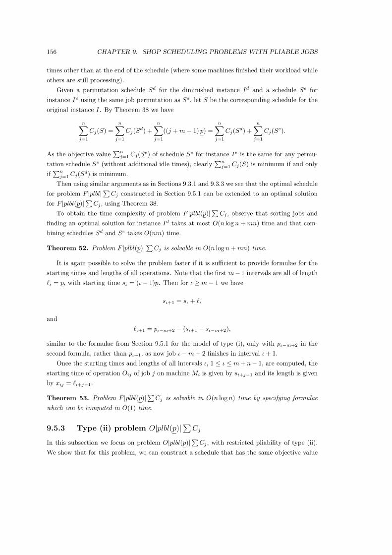
156 CHAPTER 9. SHOP SCHEDULING PROBLEMS WITH PLIABLE JOBS
times other than at the end of the schedule (where some machines finished their workload while
others are still processing).
Given a permutation schedule Sd for the diminished instance Id and a schedule Se for
instance Ie using the same job permutation as Sd, let S be the corresponding schedule for the
original instance I. By Theorem 38 we have
n∑j=1
Cj(S) =
n∑j=1
Cj(Sd) +
n∑j=1
((j +m− 1) p) =
n∑j=1
Cj(Sd) +
n∑j=1
Cj(Se).
As the objective value∑nj=1 Cj(S
e) of schedule Se for instance Ie is the same for any permu-
tation schedule Se (without additional idle times), clearly∑nj=1 Cj(S) is minimum if and only
if∑nj=1 Cj(S
d) is minimum.
Then using similar arguments as in Sections 9.3.1 and 9.3.3 we see that the optimal schedule
for problem F |plbl|∑Cj constructed in Section 9.5.1 can be extended to an optimal solution
for F |plbl(p)|∑Cj , using Theorem 38.
To obtain the time complexity of problem F |plbl(p)|∑Cj , observe that sorting jobs and
finding an optimal solution for instance Id takes at most O(n log n+mn) time and that com-
bining schedules Sd and Se takes O(nm) time.
Theorem 52. Problem F |plbl(p)|∑Cj is solvable in O(n log n+mn) time.
It is again possible to solve the problem faster if it is sufficient to provide formulae for the
starting times and lengths of all operations. Note that the first m− 1 intervals are all of length
`ι = p, with starting time sι = (ι− 1)p. Then for ι ≥ m− 1 we have
sι+1 = sι + `ι
and
`ι+1 = pι−m+2 − (sι+1 − sι−m+2),
similar to the formulae from Section 9.5.1 for the model of type (i), only with pι−m+2 in the
second formula, rather than pι+1, as now job ι−m+ 2 finishes in interval ι+ 1.
Once the starting times and lengths of all intervals ι, 1 ≤ ι ≤ m+ n− 1, are computed, the
starting time of operation Oij of job j on machine Mi is given by si+j−1 and its length is given
by xij = `i+j−1.
Theorem 53. Problem F |plbl(p)|∑Cj is solvable in O(n log n) time by specifying formulae
which can be computed in O(1) time.
9.5.3 Type (ii) problem O|plbl(p)|∑Cj
In this subsection we focus on problem O|plbl(p)|∑Cj , with restricted pliability of type (ii).
We show that for this problem, we can construct a schedule that has the same objective value

9.5. TYPE (I) AND TYPE (II) PROBLEMS WITH MIN-SUM CRITERIA 157
as an optimal schedule for problem P |pmtn|∑Cj . Clearly, such a schedule must be optimal
also for O|plbl(p)|∑Cj .
First we introduce the notion of a Latin square, see, e.g., [25]. A Latin square is an m×marray filled with m different numbers such that each number appears exactly once in every row
and every column. In an instance with m machines, we construct the schedule as a sequence
of m×m Latin squares of operations of m jobs, where the rows of the Latin squares represent
the different machines and the columns represent the order of operations on the machines.
Let the jobs be numbered in order of non-decreasing processing times. On each machine,
the first and the last operation of each Latin square may be longer, while all m− 2 operations
in the middle columns of the Latin square are of minimum size p. The first Latin square is
constructed for jobs 1, 2, . . . ,m, the second is constructed for jobs m + 1,m + 2, . . . , 2m, etc.
such that the k-th Latin square is constructed for jobs (k − 1)m + 1, (k − 1)m + 2, . . . , km. If
the number of jobs is not a multiple of the number of machines, then in the last Latin square
some jobs are missing.
It is sufficient to consider only two Latin squares, one tying into the other, and construct the
schedule alternating between the two chosen Latin squares. Any combination of Latin squares
L1 and L2 such that the first column of L1 is equal to the last column of L2 and the last
column of L1 is equal to the first column of L2 would work. In what follows we use the two
Latin squares of the form
L1 =
1 2 3 . . . m− 1 m
m 1 2 . . . m− 2 m− 1
m− 1 m 1 . . . m− 3 m− 2...
.... . .
. . ....
...
3 4 5 . . . 1 2
2 3 4 . . . m 1
,
and
L2 =
m m− 1 m− 2 . . . 2 1
m− 1 m− 2 m− 3 . . . 1 m
m− 2 m− 3 m− 4 . . . m m− 1...
.... . .
. . ....
...
2 1 m . . . 4 3
1 m m− 1 . . . 3 2
Note that L2 uses the same columns as L1 in reversed order.
When constructing the schedule, we first assign all minimum length operations of jobs
1, 2 . . . ,m to the machines in the structure given by L1, i.e. such that the sequence of operations
on machine Mi is equal to the i-th line of L1. In order to make sure the full processing time
of each job is scheduled, we lengthen the last operation of each job (the operations represented

158 CHAPTER 9. SHOP SCHEDULING PROBLEMS WITH PLIABLE JOBS
by the last column of the Latin square). Thus, jobs 1, . . . ,m have m− 1 minimum operations
in the beginning of the schedule, and then one operation of length pj − (m − 1)p on the last
machine on which they appear, see Fig. 9.10.
Figure 9.10: The start of a schedule for problem O|plbl(p)|∑Cj
Now we schedule all minimum length operations of the next m jobs, jobs m+1,m+2, . . . , 2m,
in the structure given by L2, starting at time pm, when the last operation of the previous Latin
square finishes. Note that this means that the last operation of job j, 1 ≤ j ≤ m, is scheduled
on the same machine as the first operation of job m+ j, see Fig. 9.11.
Figure 9.11: Adding the second Latin square of operations
Again, as the second step we lengthen the operations of the Latin square in order to make
sure all processing time is scheduled. This time, where possible, we first lengthen the operations
in the first column (the first operations of jobs m+ 1, m+ 2, . . ., 2m), such that there are no
idle times left on any machine. This is possible, because the jobs are numbered according to
non-decreasing processing times, and therefore pj ≥ pm for all jobs j > m. In a second step,
we lengthen the operations in the last column (as we did for the first Latin square) to schedule
all remaining processing time, see Fig. 9.12.

9.5. TYPE (I) AND TYPE (II) PROBLEMS WITH MIN-SUM CRITERIA 159
Figure 9.12: A complete schedule for problem O|plbl(p)|∑Cj with 8 jobs
If we continue to construct the schedule in this manner, it is easy to see that we end up
with completion times C1 = p1, C2 = p2, . . ., Cm = pm and Cj = pj + Cj−m for j > m. Again
we meet the lower bound for P |pmtn|∑Cj and thus the constructed schedule is optimal.
The schedule can be constructed in such a way that only two different, pre-set Latin squares
are needed, one tying into the other as described above. For each job, only the lengths of the
first and the last operations need to be computed, all other operations are of minimum length.
For jobs j, j ≤ m, the first operation is of minimum length p and the last operation is of length
pj − (m − 1)p. If instead (k − 1)m < j ≤ km for some k ≥ 2 and job j is processed within
the k-th Latin square, then the first operation of job j has length C(k−1)m−Cj−m and the last
operation of job j has length pj − (C(k−1)m − Cj−m + (m− 2)p).
The completion times of all job can be computed recursively in O(n) using the formula
for the corresponding parallel machine problem, after sorting the jobs in SPT order. Once
the completion times of all jobs are known, computing the lengths of the first and the last
operations of all jobs with the formulas above again takes O(n) time, O(1) time for each
individual operation.
The schedule as a whole can be computed in O(n log n+mn) time, including the sorting of
the jobs, and the computation and output of starting and completion times for mn non-zero
operations.
Theorem 54. Problem O|plbl(p)|∑Cj is solvable in O(n log n+mn) time.
9.5.4 Other problems with min-sum criteria
In this section we give a brief overview of other traditional min-sum criteria, namely weighted
sum of completion times, number of late jobs, weighted number of late jobs, total tardiness and
weighted total tardiness. Recall that by Theorem 35 for any such objective f problems O|plbl|fand F |plbl|f with the number of machines part of the input are at least ordinarily NP-hard.

160 CHAPTER 9. SHOP SCHEDULING PROBLEMS WITH PLIABLE JOBS
Weighted sum of completion times
By Theorem 35 problems O2|plbl|∑wjCj and F2|plbl|∑wjCj are NP-hard in the ordinary
sense and problems O|plbl|∑wjCj and F |plbl|∑wjCj are strongly NP-hard.
Problem Om|plbl|∑wjCj is pseudo-polynomially solvable in O(mn (∑pj)
m−1) time with
the known algorithm for Pm|pmtn|ΣwjCj (see [97]). Using the same algorithm in combination
with the results from [123], we can also solve Fm|plbl|∑wjCj in T (n,m) +O(mn (∑pj)
m−1)
time, where T (n,m) is the time it takes to solve the LP from [123], see Section 9.1.1.
It is difficult to generalize these results to the model with a common lower bound of type
(ii). An approach using the methodology from Section 9.1.2, where we first split an instance I
into an diminished instance Id and an instance Ie where all processing times are equal to mp
and then combine two optimal permutation schedules with the same job order, does not work.
In Section 9.5.2 we could use such an approach, since the objective value of a permutation
schedule for instance Ie was independent of the permutation used. However, this is no longer
the case if weights are introduced. Therefore the optimal permutation schedule for instance
Ie may not have the same job order as an optimal permutation schedule for the diminished
instance Id, and the two schedules cannot be combined.
For a slightly different reason the approach from Section 9.5.3 also cannot be generalized
in an obvious way. The problem here is that the sequence of jobs for an optimal solution of
weighted sum of completion times is not necessarily in order of non-decreasing processing times.
Thus it can no longer be guaranteed that operations can be lengthened to make sure no idle
times appear in the schedule.
Number of late jobs
Problem P |pmtn|∑Uj is NP-hard in the ordinary sense (see, e.g., [17, 97]) and thus the same
is true for problems O|plbl|∑Uj and F |plbl|∑Uj by Theorem 35. We do not investigate the
possibility of a pseudo-polynomial time algorithm since the existence of such an algorithm for
P |pmtn|∑Uj is still open, to the best of our knowledge, and the answer to this question is
beyond the scope of this thesis.
On the other hand problem Pm|pmtn|∑Uj with a fixed number of machines is polynomially
solvable and the algorithm produces an O-type schedule (up to zero-length operations in the
beginning of the schedule) in O(n3(m−1)) time (see [97]). Hence, Om|plbl|∑Uj can be solved
in O(n3(m−1)) time.
In order to solve problem Fm|plbl|∑Uj we need a slightly different approach than for
problem Fm|plbl|∑wjCj in the previous section, since∑Uj is not continuous, and therefore
the LP from [123] cannot be used directly to transform a schedule for problem Pm|pmtn|∑Uj
into an F -type schedule. Recall, however, that the structural result in [123] still shows that an
optimal F -type schedule exists for problem Fm|plbl|∑Uj (see also Theorem 34). Note further
that there exists an optimal schedule in which all jobs, which are on time, finish before any late

9.5. TYPE (I) AND TYPE (II) PROBLEMS WITH MIN-SUM CRITERIA 161
job finishes (this is also shown in Lemma 55 for the more general model of type (ii)). Thus we
can consider the on time jobs separately from the late jobs.
We solve problem Fm|plbl|∑Uj in two steps. First we use the known algorithm for problem
Pm|pmtn|∑Uj in order to identify the optimal set N1 ⊆ J of on time jobs in O(n3(m−1)) time
[97].
Now consider only the job in N1. Due to the structural result in [123] there exists an F -
type schedule where all jobs in N1 are on time. Treating the due dates of the on time jobs as
deadlines, we can find such an F -type schedule S using the algorithm in [11], see also Section
9.2.2. This is the same as finding a schedule of maximum lateness Lmax ≤ 0 for the sub-instance
given by the set of jobs N1.
We extend S by scheduling all late jobs j ∈ J \N1 at the end of S in any order, such that
the conditions for feasibility and F -type are fulfilled. In total, problem Fm|plbl|∑Uj can be
solved in O(n3(m−1) +mn+ n log n) = O(n3(m−1)) time, assuming m ≥ 2 and n ≥ m.
For problem O|plbl(p)|∑Uj of type (ii), it is unclear whether the result from the model
with unrestricted pliability can be generalized. Indeed, for open shop even the easier problem
with the makespan objective is still unsolved, as discussed earlier in Section 9.3.2.
In contrast to that a generalization is again possible for the flow shop version. First we extend
the observation we made for the structure of an optimal schedule of problem Fm|plbl|∑Uj to
the model with equal but non-zero lower bounds.
Lemma 55. For problem F |plbl(p)|∑Uj there exists an optimal permutation schedule, in
which first all on time jobs are scheduled in non-decreasing order of due-dates, and then all late
jobs.
Proof: An optimal permutation schedule exists by Theorem 37. If it is not of the desired form,
we use adjacent jobs swaps (Lemma 36) to reorder the jobs accordingly. We can see that no
additional late jobs are created with arguments similar to the arguments used for Lemma 46.
Thus, if the set of on time jobs N1 ⊆ J is known, then we can solve problem Fm|plbl(p)|Lmax
for the jobs in N1, obtaining a schedule where all these jobs are on time. Then in a second step
we add the late jobs to the end of the schedule, in any order.
In order to show that problem Fm|plbl(p)|∑Uj is solvable in O(n3(m−1)) time, we prove
the following theorem.
Lemma 56. Let I be an instance of problem F |plbl(p)|∑Uj and let Id be the diminished
instance as defined in Section 9.3.3. Then, given a subset N1 ⊆ J of the set of jobs, there
exists a schedule S for instance I in which all jobs of set N1 are on time, if and only if there
exists a schedule Sd for instance Id in which all jobs corresponding to the jobs in N1 are on
time.
Proof: Construct an instance Isub of problem F |plbl(p)|Lmax with job set N1. Denote the
corresponding diminished instance by Idsub.

162 CHAPTER 9. SHOP SCHEDULING PROBLEMS WITH PLIABLE JOBS
Note first that there exists a schedule for instance I in which all jobs in set N1 are on time
if and only if there exists a schedule for instance Isub with Lmax ≤ 0. A similar observation can
be made for instances Id and Idsub.
Furthermore, since the diminished instance Idsub of Isub is constructed similarly to the con-
struction in Section 9.3.3, the optimal Lmax-values for Isub and Idsub are equal, see (9.11). Thus,
a schedule with Lmax ≤ 0 exists for instance Isub if and only if one exists for Idsub.
Therefore, the following four statements are equivalent:
1. there exists a schedule S for instance I in which all jobs in set N1 are on time,
2. there exists a schedule Ssub for instance Isub with Lmax ≤ 0,
3. there exists a schedule Sdsub for instance Idsub with Lmax ≤ 0,
4. there exists a schedule Sd for instance Id in which all jobs in set N1 are on time.
The equivalence of the first and fourth statement proves the lemma.
Using Lemmas 55 and 56 we can solve problem Fm|plbl(p)|∑Uj in the following way. Given
instance I construct the diminished instance Id as defined in Section 9.3.3. Use the algorithm
for problem Fm|plbl|∑Uj to solve instance Id optimally, obtaining a maximum set of on time
jobs Nd1 . By Lemma 56, the set N1 of jobs corresponding to the jobs in Nd
1 is a maximum set
of on time jobs for instance I.
As the second step, solve problem Fm|plbl(p)|Lmax for the instance with job set N1, ob-
taining a schedule with Lmax ≤ 0. Finally, extend the schedule to a schedule for instance I by
adding at the end, feasibly, all jobs in set J \N1.
The first step, solving Fm|plbl|∑Uj for the diminished instance Id, takes O(n3(m−1)) time.
After that, solving problem Fm|plbl(p)|Lmax takes no longer than O(n log n + mn) time and
adding the jobs in set J \ N1 at the end of the schedule takes no longer than O(mn) time.
Therefore the total runtime of the algorithm is O(n3(m−1)).
Theorem 57. For all m ≥ 2 problem Fm|plbl(p)|∑Uj is solvable in O(n3(m−1)) time.
Weighted number of late jobs, total tardiness and weighted total tardiness
It is well known that problems 1|pmtn|∑Tj and 1|pmtn|∑wjUj are NP-hard in the ordinary
sense and that problem 1|pmtn|∑wjTj is strongly NP-hard (see, e.g., [17], [97]). Therefore, by
Theorem 35, problems F2|plbl|∑Tj , O2|plbl|∑Tj , F2|plbl|∑wjUj and O2|plbl|∑wjUj are
NP-hard in the ordinary sense and problems F2|plbl|∑wjTj and O2|plbl|∑wjTj are strongly
NP-hard.
It is open whether P2|pmtn|∑Tj is solvable in pseudo-polynomial time [17, 97], so we do
not attempt to answer the question for strong NP-hardness for problems O2|plbl|∑Tj and
F2|plbl|∑Tj here. On the other hand, problem Pm|pmtn|∑wjUj is solvable in pseudo-
polynomial time, more precisely in O(n3m−5 (
∑wi)
2)
time for m ≥ 3 and O(n2 (
∑wi))
for

9.6. PROOF OF LEMMA 36 163
m = 2. Again, the algorithms produce an O-type solution up to zero-length operations, see
[97, 98]. Thus problem Om|plbl|∑wjUj is pseudo-polynomially solvable with the same time
complexity.
For problems Fm|plbl|∑wjUj and Fm|plbl(p)|∑wjUj we can use the same idea as in
the previous section: first solve the related parallel machine problem to find out the op-
timal set N1 of on time jobs (after creating the diminished instance in the case of prob-
lem Fm|plbl(p)|∑wjUj), then solve problem Fm|plbl(p)|Lmax or Fm|plbl(p)|Lmax respec-
tively to obtain a schedule in which all jobs of set N1 are on time. Consequently, problems
Fm|plbl|∑wjUj and Fm|plbl(p)|∑wjUj are pseudo-polynomially solvable with the same time
complexity as the associated preemptive parallel machine problem.
9.6 Proof of Lemma 36
Consider problem F |plbl(p)|f and two permutation schedules S and S′, as described in the
formulation of Lemma 36. These two schedules differ in allocation of jobs u and v, while the
remaining jobs are kept unchanged.
Given schedule S, we perform the following preprocessing. Introduce time windows [`i, ri]
on every machine Mi, 1 ≤ i ≤ m, available for processing u, v, where `i is the completion
time of the last operation on machine Mi that precedes job u in S and ri corresponds to the
starting time of the first operation on machine Mi that follows job v in S. Having fixed windows
[`i, ri], we exclude from consideration jobs J \u, v. An example of schedule S is presented in
Fig. 9.13, where we mark compulsory parts of jobs u, v, each of length p, by dotted boxes.
Time windows [`i, ri] can be narrowed down to [`′i, r′i] ⊆ [`i, ri] excluding subintervals which
remain idle in any feasible schedule:
`′1 = `1, `′i = max`i, `
′i−1 + p
, i = 2, 3, . . . ,m,
r′m = rm, r′i = minri, r
′i+1 − p
, i = m− 1,m− 2, . . . , 1.
(9.17)
In Fig. 9.13, the adjustment of r1 excludes from consideration idle interval [r′1, r1], which cannot
be used on machine M1, while the adjustment of `2 excludes idle interval [`2, `′2], which cannot
be used on machine M2, whichever job order is fixed, u preceding v on all machines or another
way around.
Additionally, schedule S can be decomposed into subschedules defined over machine sets
M1, . . . ,Mi−1 and Mi, . . . ,Mm, if
`′i + p ≥ r′i−1 (9.18)
for some 2 ≤ i ≤ m; see Fig. 9.13 with i = 4 and machine sets M1,M2,M3 and M4,M5.Here condition (9.18) ensures that for the fixed job order, with u preceding v, allocating the
compulsory part of job v in[r′i−1 − p, r′i−1
]on machine Mi−1 and allocating the compulsory
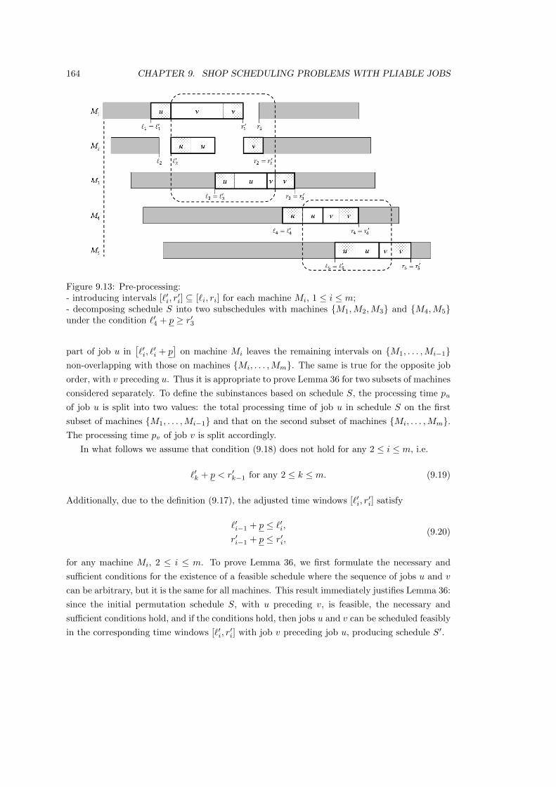
164 CHAPTER 9. SHOP SCHEDULING PROBLEMS WITH PLIABLE JOBS
Figure 9.13: Pre-processing:- introducing intervals [`′i, r
′i] ⊆ [`i, ri] for each machine Mi, 1 ≤ i ≤ m;
- decomposing schedule S into two subschedules with machines M1,M2,M3 and M4,M5under the condition `′4 + p ≥ r′3
part of job u in[`′i, `
′i + p
]on machine Mi leaves the remaining intervals on M1, . . . ,Mi−1
non-overlapping with those on machines Mi, . . . ,Mm. The same is true for the opposite job
order, with v preceding u. Thus it is appropriate to prove Lemma 36 for two subsets of machines
considered separately. To define the subinstances based on schedule S, the processing time pu
of job u is split into two values: the total processing time of job u in schedule S on the first
subset of machines M1, . . . ,Mi−1 and that on the second subset of machines Mi, . . . ,Mm.The processing time pv of job v is split accordingly.
In what follows we assume that condition (9.18) does not hold for any 2 ≤ i ≤ m, i.e.
`′k + p < r′k−1 for any 2 ≤ k ≤ m. (9.19)
Additionally, due to the definition (9.17), the adjusted time windows [`′i, r′i] satisfy
`′i−1 + p ≤ `′i,r′i−1 + p ≤ r′i,
(9.20)
for any machine Mi, 2 ≤ i ≤ m. To prove Lemma 36, we first formulate the necessary and
sufficient conditions for the existence of a feasible schedule where the sequence of jobs u and v
can be arbitrary, but it is the same for all machines. This result immediately justifies Lemma 36:
since the initial permutation schedule S, with u preceding v, is feasible, the necessary and
sufficient conditions hold, and if the conditions hold, then jobs u and v can be scheduled feasibly
in the corresponding time windows [`′i, r′i] with job v preceding job u, producing schedule S′.

9.6. PROOF OF LEMMA 36 165
Lemma 58. There exists a feasible schedule for scheduling jobs u and v in the same order on
machines Mi, 1 ≤ k ≤ m, within time windows [`′i, r′i] satisfying (9.19) and (9.20), if and only
the following three conditions hold:
(A) r′i − `′i ≥ 2p, 1 ≤ i ≤ m;
(B) pu + p ≤ r′m − `′1 and pv + p ≤ r′m − `′1;
(C) pu + pv ≤ T1 + 2T2, where T1 is the total time within [`′1, r′m] when exactly one of the
machines M1,M2, . . . ,Mm is available, and T2 is the total time within the same interval
when at least two machines are available.
Proof of Lemma 58: Without loss of generality we consider a fixed job order with u preceding
v.
“⇒”: We show that if one of the conditions is violated, then a feasible schedule cannot be
achieved. Indeed, if (A) does not hold for some machine Mi, then the two operations of jobs u
and v of the minimum length p cannot be scheduled.
If the first inequality from (B) does not hold, then the whole interval [`′1, r′m] cannot fit the
full processing amount pu of job u, distributed over m machines, together with the minimum
amount p of job v allocated to Mm. Similarly, if the second inequality from (B) does not hold,
then [`′1, r′m] cannot fit the full processing amount pv of job v, distributed over m machines,
together with the minimum amount p of job u allocated to M1.
Finally, if (C) does not hold, then the relaxed problem, with m identical parallel machines
processing two jobs with preemption, does not have a feasible solution.
“⇐”: Suppose now that (A), (B), (C), (9.20) and (9.19) hold. We formulate an algorithm that
finds a feasible schedule with u preceding v on every machine.
The algorithms starts with splitting [`′1, r′m] into intervals of two types, I1 and I2: within
any I1-interval exactly one of the machines M1,M2, . . . ,Mm is available and within any I2-
interval at least two machines are available. Note that parameters T1 and T2 that appear in
condition (C) of the lemma correspond to the combined lengths of I1-intervals and I2-intervals,
respectively. Moreover, by (9.19), any time point within [`′1, r′m] falls into one of these two
categories, so that
T1 + T2 = r′m − `′1. (9.21)
Since the set of available intervals starts with an I1-type interval of size at least p and
finishes with an I1-type interval, also of size at least p,
T1 ≥ 2p. (9.22)
Perform (temporarily) an additional adjustment of the problem instance, increasing pu, pv
to the maximum combined value
p′u + p′v = T1 + 2T2, (9.23)

166 CHAPTER 9. SHOP SCHEDULING PROBLEMS WITH PLIABLE JOBS
and making sure that p′u and p′v satisfy the following two additional inequalities:
p′u ≥ p+ T2, (9.24)
p′v ≥ p+ T2. (9.25)
The extra amount of processing (p′u + p′v)− (pu + pv) will be removed from a feasible schedule
after it is constructed. To demonstrate the existence of p′u, p′v satisfying (9.23)-(9.25), assume
without loss of generality that the initial processing times satisfy
pu ≥ pv (9.26)
and consider the following possible set of new processing times:
p′u = pu, p′v = T1 + 2T2 − pu, if pu ≥ p+ T2,
p′u = p+ T2, p′v = T1 + T2 − p, if pu < p+ T2.
Notice that
– p′u ≥ pu, i.e., the processing time of job u does not decrease;
– condition p′v ≥ pv holds due to (C) in the first case and due to (9.22) and (9.26) in the
second case, i.e., the processing time of job v does not decrease;
– (9.23) and (9.24) are satisfied in both cases;
– the validity of (9.25) in the first case follows from (9.21) combined with the first inequality
from (B), and its validity in the second case follows from (9.22).
The algorithm for allocating jobs u and v which satisfy (9.23)-(9.25) starts with intervals of
type I2, making sure that each of the jobs u and v is continuously processed in these intervals.
Denote by pij(I2) the amount of processing of job j ∈ u, v allocated to machine Mi in an
I2-type interval and define:
p1u(I2) = 0, p1v(I2) = r′1 − `′2,piu(I2) = min
r′i−1, `
′i+1
− `′i, piv(I2) = r′i −max
r′i−1, `
′i+1
, i = 2, . . . ,m− 1,
pmu(I2) = r′m−1 − `′m, pmv(I2) = 0.
An illustrative example is presented in Fig. 9.14, where I1- and I2-intervals are marked by
single-line and double-line rounded frames. It is easy to verify that the following properties
hold for the given partial allocation:
– machines M1 and Mm process only one job, u or v;
– every remaining machine Mi, 2 ≤ i ≤ m− 1, processes job u first and job v next;
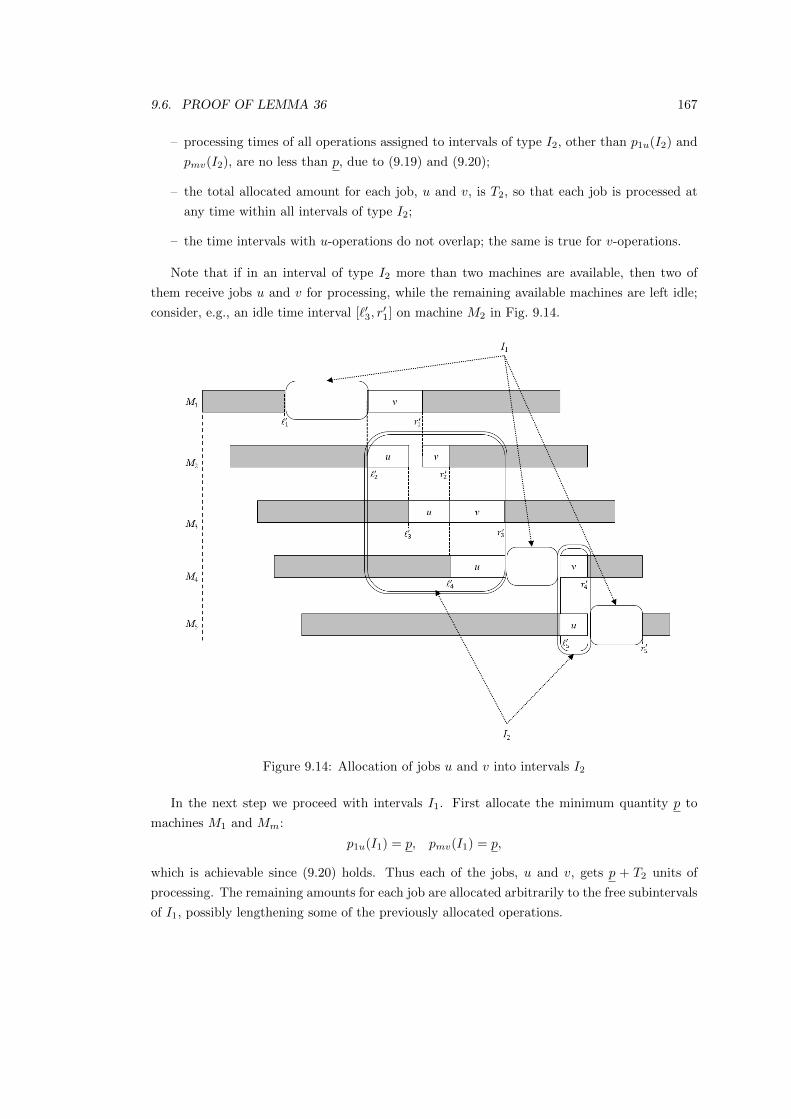
9.6. PROOF OF LEMMA 36 167
– processing times of all operations assigned to intervals of type I2, other than p1u(I2) and
pmv(I2), are no less than p, due to (9.19) and (9.20);
– the total allocated amount for each job, u and v, is T2, so that each job is processed at
any time within all intervals of type I2;
– the time intervals with u-operations do not overlap; the same is true for v-operations.
Note that if in an interval of type I2 more than two machines are available, then two of
them receive jobs u and v for processing, while the remaining available machines are left idle;
consider, e.g., an idle time interval [`′3, r′1] on machine M2 in Fig. 9.14.
Figure 9.14: Allocation of jobs u and v into intervals I2
In the next step we proceed with intervals I1. First allocate the minimum quantity p to
machines M1 and Mm:
p1u(I1) = p, pmv(I1) = p,
which is achievable since (9.20) holds. Thus each of the jobs, u and v, gets p + T2 units of
processing. The remaining amounts for each job are allocated arbitrarily to the free subintervals
of I1, possibly lengthening some of the previously allocated operations.

168 CHAPTER 9. SHOP SCHEDULING PROBLEMS WITH PLIABLE JOBS
In the resulting schedule all intervals of type I1 and I2 are used as much as possible, with
exactly one job processed at any time within I1 and two jobs processed at any time within I2.
Thus the total processing time of jobs u and v is T1 + 2T2 and both jobs are scheduled in full.
If processing times have been extended to achieve (9.23), then the constructed schedule
should be modified by reducing the operations with lengths larger than p, without violating
this lower bound. Note that in a feasible instance for problem F |plbl(p)|f , each job j ∈ N
satisfies pj ≥ mp.The described algorithm constructs a feasible schedule with u preceding v, if conditions
(A)-(C) and (9.20)-(9.19) hold. Since these conditions are symmetric with respect to pu and
pv, the proposed algorithm can be used to construct a feasible schedule with v preceding u, as
stated in Lemma 36.

Chapter 10
Conclusions and further research
The results we obtained for flow shop and open shop scheduling with pliable jobs are summarized
in Tables 10.1-10.2. For comparison, we provide the related results for traditional models, with
and without preemption (for references see [17] and/or Chapter 2.3 of this thesis). We do not
perform the comparison with the lot streaming model, as that model is less related to the model
with pliable jobs. Note that the complexity result for problem F |plbl(p)|Cmax is given under
the assumption that the trivial part of the schedule, which consists only of minimum length
operations, does not need to be computed.
Problem: trad. trad. pliability modelmodel, model, plbl plbl(p) plbl(p
ij, pij)
no pmtn pmtn (i) (ii) (iii)
O2||Cmax O(n) O(n) O(n) O(n) O(n)Th. 40,49 Th. 49 Th. 49
F2||Cmax O(n log n) O(n log n) O(n) O(n) NP-h.Th. 40 Th. 43 Th. 48
Om||Cmax NP-h. O(n2) O(n) open NP-h.(m ≥ 3),(m ≥ 3), Th. 40 Sect. 9.1.3
Fm||Cmax sNP-h. sNP-h. O(n) O(n) sNP-h.(m ≥ 3)(m ≥ 3) (m ≥ 3) Th. 40 Th. 43 Sect. 9.1.3
O||Cmax sNP-h. O(n2m2) O(n) open sNP-h.,Th. 40 Sect. 9.1.3
F ||Cmax sNP-h. sNP-h. O(n) O(n) sNP-h.Th. 40 Th. 43 Sect. 9.1.3
O||Lmax sNP-h. LP O(n log n) open sNP-h.(m ≥ 2)(m ≥ 2) Th. 42 Sect. 9.1.3
F ||Lmax ” ” ” sNP-h. O(n log n+mn) O(n log n+mn) ” ” ”(m ≥ 2) Th. 42 Th. 47
Table 10.1: Open shop and flow shop problems with pliable jobs and minmax objectives
169

170 CHAPTER 10. CONCLUSIONS AND FURTHER RESEARCH
Problem: trad. trad. pliability modelmodel, model, plbl plbl(p) plbl(p
ij, pij)
no pmtn pmtn (i) (ii) (iii)
O||ΣCj sNP-h. NP-h. O(n log n) O(n log n+ nm) sNP-h.(m ≥ 2)(m ≥ 2) (m ≥ 2) Th. 51 Th. 54 Sect. 9.1.3
F ||ΣCj ” ” ” sNP-h. O(n log n+ nm) O(n log n+ nm) ” ” ”(m ≥ 2) Th. 50 Th. 52
Om||ΣwjCj sNP-h. sNP-h. both NP-h. both NP-h. sNP-h.(m ≥ 2)(m ≥ 2) (m ≥ 2) (pseudo- (open whether Sect. 9.1.3
Fm||ΣwjCj ” ” ” ” ” ” poly. solv.) strongly) ” ” ”Sect. 9.5.4 Sect. 9.5.4
O||ΣwjCj sNP-h. sNP-h. sNP-h. sNP-h. sNP-h.Th. 35 Th. 39 Sect. 9.1.3
F ||ΣwjCj ” ” ” ” ” ” ” ” ” ” ” ” ” ” ”
Om||ΣUj sNP-h. NP-h. O(n3(m−1)
)open sNP-h.(m ≥ 2)
(m ≥ 2) (m ≥ 2) Sect. 9.5.4 Sect. 9.1.3Fm||ΣUj ” ” ” sNP-h O
(n3(m−1)
)O(n3(m−1)
)” ” ”
(m ≥ 2) Sect. 9.5.4 Th. 57O||ΣUj sNP-h. NP-h. NP-h. NP-h. sNP-h.
Th. 35 Th. 39 Sect. 9.1.3F ||ΣUj ” ” ” sNP-h. ” ” ” ” ” ” ” ” ”
Table 10.2: Open shop and flow shop problems with pliable jobs and minsum objectives
10.1 General observations
As a rule, the problems with unrestricted pliability of type (i) appear to be no harder than their
counterparts for the traditional model, with or without preemption, and are often solvable by
faster algorithms than the traditional ones. This is due to the strong relation to the parallel
machine with preemption discussed in Section 9.1.1.
Contrarily, due to the reductions in Theorem 39, the problems with restricted pliability of
type (iii) are no easier than their traditional counterparts. Additionally, the type (iii) prob-
lem F2|plbl(pij, pij)|Cmax is NP-hard while its classical counterpart F2||Cmax is solvable in
O(n log n) time (see [79]).
Comparing open shop and flow shop models, we observe that for pliability of type (i) open
shop models have the same time complexity as flow shop models for all traditional objec-
tive functions f , other than Lmax and∑Cj , where they are slightly easier. On the other
hand, surprisingly, for pliability of type (ii) open shop models cause considerable problems
and we were forced to leave them open for the problems O|plbl(p)|Cmax, O|plbl(p)|Lmax and
Om|plbl(p)|∑Uj . Note that corresponding flow shop problems are polynomially solvable. Fi-
nally, for pliability of type (iii), open shop models and flow shop models have mostly the same
complexity status. The only major deviation from this rule is that problem F2|plbl(pij, pij)|Cmax
is NP-hard while problem O2|plbl(pij, pij)|Cmax is solvable in linear time.

10.2. PLIABILITY OF TYPE (I) AND (II) WITH N < M 171
10.2 Pliability of type (i) and (ii) with n < m
We performed the complexity analysis for the case n ≥ m. If the number of machines m is
larger than the number of jobs n, n < m, then many of the algorithms for the models with
pliability of type (i) and (ii) can be simplified. For the open shop models of type (i) we can
schedule the full processing time of each job on a different machine, with zero-length operations
on all other machines in the beginning of the schedule. Since in the described schedule the
completion time of each job is equal to its processing time, such a schedule is optimal for every
regular objective function.
For the flow shop models of type (i) we can use the same idea, only that we have to schedule
jobs such that the shortest job is fully processed by the last machine, the second shortest by the
second to last machine and so on. Zero-length operations can be added in such a way that the
schedule is of permutation type, with jobs in SPT order on each machine. Job j has m−j zero-
length operations on machines M1,M2, . . . ,Mm−j , followed by an operation of length pj on ma-
chine Mm−j+1 and finally j−1 zero-length operations on machines Mm−j+1,Mm−j+2, . . . ,Mm,
finishing at time pj on machine Mm. Again, in the described schedule the completion time of
each job is equal to its processing time.
For models with pliability of type (ii) we adjust the above schedules to respect the require-
ment that all operations have to be at least of length p. For the open shop schedule, we schedule
m− 1 operations of length p for each job, then schedule the remaining processing time fully on
one machine. Since m > n and therefore m − 1 ≥ n, the first part of the schedule, with the
minimum length operations, takes (m − 1)p time. It can be thought of as m − 1 synchronous
cycles, each of length p (see Chapter 3). Each job is scheduled in every cycle, but machines
may be idle in one or several cycles. After that, a job j has pj − (m− 1)p processing time left,
which is all scheduled on the one machine that it has not yet visited. Consequently, each job j
is processed continuously from time 0, finishing at time pj . As before, the described schedule
is optimal for every regular objective.
Lastly, for flow shop models of type (ii), the situation is slightly more complicated. Note first
that Theorem 37 is independent of the relation between n and m and thus optimal permutation
schedules exist. Assume a permutation of the jobs is given and jobs are numbered in order of
that permutation. We construct a permutation schedule with jobs in the given permutation
on all machines by scheduling m− 1 minimum length operations of the first job, m− 2 of the
second, and so on, similar to the beginning part of the schedule in Fig. 9.2. Job j has m − jminimum length operations scheduled in that part. Then, in the middle part of the schedule
each job has one operation of length pj − (m− 1)p scheduled on machine Mm−j+1. Then, the
remaining minimum length operations of each job are scheduled on the downstream machines,
starting as early as possible without violating the given permutation or any of the feasibility
constraints.
In the constructed schedule, job 1 finishes at time p1, job 2 at time maxp1 + p, p2 + p, job

172 CHAPTER 10. CONCLUSIONS AND FURTHER RESEARCH
3 at time maxp1 + 2p, p2 + 2p, p3 + 2p, and in general job j, 1 ≤ j ≤ n, at time
Cj = maxpu + (j − 1)p|u ≤ j. (10.1)
Clearly, if the permutation of jobs on each machine is equal to the given permutation (the
numbering of jobs), then no job can finish earlier and the splitting of the jobs is optimal for the
given permutation and any regular objective.
Thus, the scheduling problem reduces to finding an optimal permutation of the jobs. For
the makespan objective we can choose any permutation, as the completion time of the last job
is always maxpj |j ∈ J + (n − 1)p. For the total sum of completion times, jobs should be
scheduled in SPT order, so that each job j finishes at time pj + (j − 1)p. For the maximum
lateness objective the jobs should be sequenced in EDD order, by the same arguments as in
Lemma 46. The optimal permutation to minimize the number of late jobs can be found using
the same method as for the single machine problem [17, 115]. Starting with the jobs numbered
in EDD order, if job j0 is the first late job, move the job j ≤ j0 with the largest processing
time to the end of the schedule (as a late job) and renumber jobs accordingly. Proceed in this
manner until all jobs that were not moved are on time.
For the other traditional scheduling objectives, finding an optimal permutation appears to be
harder. In general, the problem of finding an optimal permutation can be treated as a sequencing
problem with completion times given by (10.1). Note that the completion times given by (10.1)
are normally smaller than they would be for a single machine sequencing problem. However, it
is unclear whether this makes it any easier or harder to obtain an optimal sequence.
To conclude this section, if n < m, we are still able solve all problems that we can solve for
the case n ≥ m. Moreover, the structure of an optimal solution becomes much simpler in the
case where n < m, as usually only one machine processes more than the minimum amount of
processing time. Open shop problems of type (i) can be solved in O(n) time for any traditional
objective function, and flow shop problems of type (i) in O(n log n) time (O(n) time for the
makespan objective).
For models of type (ii), if the trivial parts of the schedules with only minimum length
operations, are obtained by some form of pre-processing (e.g. pre-set templates), then the
open shop problem with any traditional objective function can again be solved in O(n) time.
Furthermore note that in the usual case, n ≥ m, we were unable to fully solve the open shop
problem with pliability of type (ii), even for the makespan objective. The flow shop model
of type (ii) can be solved in O(n) time for the makespan objective, and O(n log n) time for
objectives Lmax,∑Cj and
∑Uj . Thus all problems solvable for the usual case, n ≥ m, are
also solvable for the case n ≤ m. Due to the very easy structure of an optimal schedule, it also
appears to be possible to specify the schedules in terms of formulae, similar to the approach in
Sections 9.3.1, 9.5.1 and 9.5.2.

10.3. FURTHER RESEARCH 173
10.3 Further research
There are many possible directions for future research in pliability, in addition to the open
problems already discussed in this and the previous chapters. The most obvious direction is to
apply pliability to job shop and mixed shop scheduling. Mixed shop is a generalization of both
open and job shop. Practical motivation for this comes again from flexibility in manufacturing,
as for the open shop and flow shop models. It would be interesting to see how the results for
pliability of type (i) and (ii) generalize if jobs have several operations on each machine.
Since flow shop with pliability of type (iii) is at least NP-hard in the ordinary sense for
the makespan objective and in the strong sense for all other traditional objectives, even for
two machines, it would be also be useful to study heuristics. If we restrict the search space to
permutation schedules (which are not necessarily optimal for the models of type (iii)), then for
a given permutation the LP stated at the end of Section 9.4.1 can be used to find an optimal
job splitting. A heuristic could search for a good permutation, repeatedly applying the LP.
There are several extensions of the models with pliability that are worth studying further.
First of all, the natural next step from the model of type (ii) would be to investigate models
of pliability with only job dependent or only machine dependent lower bounds, i.e. pij
= pj
or pij
= pi. In the case of job dependent lower bounds it is easy to see that the NP-hardness
result from Theorem 48 still holds. Indeed, in the reduction we used to prove that theorem,
the lower bounds are only dependent on the jobs (that is 0 for jobs 1, 2, . . . n and E for job
n + 1), while upper bounds are assumed to be equal to pj for each job j. Therefore problem
F2|plbl(pij
= pj)|Cmax is at least NP-hard in the ordinary sense.
For the model with machine dependent lower bounds we appear to have a better chance
for positive results. While we do not go into detail here, initial study suggests that problem
F2|plbl(pij
= pi)|Cmax is solvable in polynomial time, by generalizing the two machine version
of the algorithm for the problem F2|plbl(p)|Cmax with pliability of type (ii). As opposed to the
model of type (ii), it seems that the permutation of jobs in an optimal schedule is no longer
arbitrary. Problems with other objectives or larger number of machines might be polynomially
solvable as well, but this is left for future study. A promising first step might be to attempt
a generalization of Theorem 37. There seems to be no obvious reason why the proofs used in
Sections 9.1.2 and 9.6 should not work for the model with machine dependent lower bounds.
Another type of pliability that seems interesting from a practical point of view can be defined
as follows. Suppose “ideal” operation lengths pij are given for each operation Oij , such that
pj =∑mi=1 pij . Given a parameter ∆ we define the upper and lower bounds on the operation
lengths for the model with pliable jobs as
pij
= pij −∆
and pij = pij + ∆(10.2)
for all 1 ≤ i ≤ m and 1 ≤ j ≤ n.

174 CHAPTER 10. CONCLUSIONS AND FURTHER RESEARCH
Similar to pliability of type (iii), all NP-hardness results from traditional open and flow shop
problems carry over, since ∆ = 0 models flow shop and open shop without pliability. However,
to prove the NP-hardness of problem F2|plbl(pij, pij)|Cmax we constructed an instance where
one job has fixed processing time on both machines (see the proof of Theorem 48). Since for
restricted pliability of the type (10.2) either ∆ = 0 and all jobs have fixed processing times on
both machines or ∆ > 0 and no job has fixed processing time on any machine, this proof is no
longer applicable. In the former case the problem becomes the traditional flow shop problem
F2||Cmax and is solvable in O(n log n) time by Johnson’s algorithm [79]. It may well be that
for restricted pliability of this type flow shop with two machines and the makespan objective is
polynomially solvable for any ∆ ≥ 0. However, at the time this thesis is written the problem is
still open.
Finally, interesting extensions of models with pliability arise when pliability is not (or not
only) restricted by lower and upper bounds, but by an additional cost of some kind. This cost
may come in form of resources, e.g. additional power needed on the machine that takes over
more than just its own workload. For an easy example of such a model consider the model
of pliability discussed in the previous paragraph, where we can make a payment to increase
parameter ∆, i.e. make our system more flexible. In other scenarios it might happen that
performing a part of the operation on a machine not specialized for it takes more time. In that
case the processing time “stretches” by some factor when we move the operation to the new
machine. For many of these models with some kind of cost, we can adjust the NP-hardness
proofs from the last chapter to show that even with no additional “hard” upper and lower
bounds for operation lengths given, they are at least as hard as the models with restricted
pliability of type (iii). Still, these models appear to be of major interest for applications and in
our opinion would be worth studying further.

Part III
Resiliency
175


Chapter 11
Definitions, notation and related
work
In this part of the thesis we propose a new approach for finding solutions to optimization
problems resilient to parameter changes. Introducing the resiliency concept for a general com-
binatorial optimization problem, we consider the area of scheduling and the famous assignment
problem as examples to illustrate the new methodology, its applicability to specific domains
and implications. Unless otherwise stated, throughout this part we assume that we deal with
minimization problems. However, similar considerations can be made for maximization prob-
lems.
As opposed to the previous two parts, the research presented here is not a closed piece of
work. Instead, it is a snap shot of work still ongoing. The main goal is to make the case that
resiliency is a concept worth further study.
11.1 Introduction
Currently the main notions used when dealing with uncertain parameters are solution stability,
sensitivity and robustness. While these concepts provide a solid theoretical justification for
decision making under uncertainty, they mainly focus on the closeness to an optimal solution
and their applicability is often limited to a relatively small class of problems. This is discussed
in more detail in Section 11.2
A natural approach to dealing with uncertainty is to produce a promising solution in advance
based on parameter estimates in order to make necessary preparations. In scheduling, for
example, it may be beneficial to prepare the system for job processing, to install required tools
and to make the set-ups. The preferred solution should keep its quality even if the actual values
of parameters differ from the original estimates. Investigating the change tolerance of solutions
is also important for scenarios where a large set of similar problems needs to be solved. In that
177
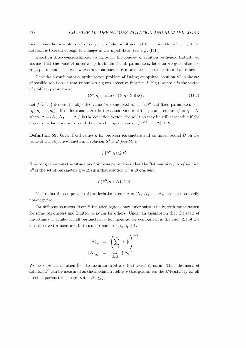
178 CHAPTER 11. DEFINITIONS, NOTATION AND RELATED WORK
case it may be possible to solve only one of the problems and then reuse the solution, if the
solution is tolerant enough to changes in the input data (see, e.g., [141]).
Based on these considerations, we introduce the concept of solution resilience. Initially we
assume that the scale of uncertainty is similar for all parameters; later on we generalize the
concept to handle the case when some parameters can be more or less uncertain than others.
Consider a combinatorial optimization problem of finding an optimal solution S∗ in the set
of feasible solutions S that minimizes a given objective function f (S, η), where η is the vector
of problem parameters:
f (S∗, η) = min f (S, η) |S ∈ S . (11.1)
Let f(S0, η
)denote the objective value for some fixed solution S0 and fixed parameters η =
(η1, η2, . . . , ηn). If under some scenario the actual values of the parameters are η′ = η + ∆,
where ∆ = (∆1,∆2, . . . ,∆n) is the deviation vector, the solution may be still acceptable if the
objective value does not exceed the desirable upper bound: f(S0, η + ∆
)≤ B.
Definition 59. Given fixed values η for problem parameters and an upper bound B on the
value of the objective function, a solution S0 is B-feasible if
f(S0, η
)≤ B.
If vector η represents the estimates of problem parameters, then theB-bounded region of solution
S0 is the set of parameters η + ∆ such that solution S0 is B-feasible:
f(S0, η + ∆
)≤ B.
Notice that the components of the deviation vector ∆ = (∆1,∆2, . . . ,∆n) are not necessarily
non-negative.
For different solutions, their B-bounded regions may differ substantially, with big variation
for some parameters and limited variation for others. Under an assumption that the scale of
uncertainty is similar for all parameters, a fair measure for comparison is the size ‖∆‖ of the
deviation vector measured in terms of some norm `q, q ≥ 1:
‖∆‖q =
n∑j=1
|∆j |q1/q
,
‖∆‖∞ = max1≤j≤n
|∆j | .
We also use the notation ‖ · ‖ to mean an arbitrary (but fixed) `q-norm. Then the merit of
solution S0 can be measured as the maximum radius ρ that guarantees the B-feasibility for all
possible parameter changes with ‖∆‖ ≤ ρ.

11.1. INTRODUCTION 179
Definition 60. A ball with center η and radius ρ is the set of values η + ∆ such that
‖∆‖ ≤ ρ.
The resiliency ball of a B-feasible solution S0 is a ball of the largest radius ρ(S0, η, B) within
the B-bounded region of S0:
ρ(S0, η, B) = maxξ|f(S0, η + ∆
)≤ B for all ‖∆‖ ≤ ξ
. (11.2)
The radius ρ(S0, η, B) is called the resiliency radius of S0. If S0 is not B-feasible, then we
define ρ(S0, η, B) = −1.
We also define the notion of a worst-case deviation for a given B-feasible solution S0.
Definition 61. Given a B-feasible solution S0, deviation ∆ is called a worst-case deviation for
S0 if ‖∆‖ = ρ(S0, η, B) and f(S0, η + ∆) = B.
Note that for different norms `q the shape of a ball varies and that the resiliency radius and
the worst-case deviation of a B-feasible solution is often dependent on the chosen norm.
To illustrate Definitions 59 and 60, consider an instance of problem 1||∑Cj . The job set
consists of two jobs with processing time estimates p1 = 3, p2 = 4, and the upper bound on the
objective value is B = 14. In solution S0 job 1 is processed first followed by job 2. Fig. 11.1
illustrates the B-bounded region, represented as a triangle, and three resiliency balls defined
for metrics `1, `2 and `∞. The deviations marked as red dots are worst-case deviations for the
respective norms. Note that the formulae for calculating the resiliency radii and worst-case
deviations are presented in Section 12.3.1.
In the presence of uncertainty, when parameter values may differ from estimates η, it is
reasonable to give preference to the most change-tolerant solution among those which are B-
feasible. The B-feasible solution S∗ with the largest resiliency radius guarantees that for the
largest size deviations solution S∗ remains B-feasible.
Definition 62. Within the set of B-feasible solutions, S∗ is the most resilient one if
ρ(S∗, η, B) = maxSρ (S, η,B) .
The radius ρmax = ρ(S∗, η, B) of the solution S∗ is called an optimum radius for the given
upper bound B.
The problem of finding the most resilient solution amongst the solutions of a given combi-
natorial optimization problem P, given an upper bound B and an estimated vector of input
parameters η, is called the resiliency version of problem P.
Above we defined solution resilience under the assumption that the scale of uncertainty
is similar for all input parameters. At the end of this introduction we define a slightly more

180 CHAPTER 11. DEFINITIONS, NOTATION AND RELATED WORK
Figure 11.1: The B-feasible region and resiliency balls for an instance of problem 1||∑Cj withp1 = 3, p2 = 4, B = 14, and solution S0 = (1, 2)
general version of resiliency. In this version, different input parameters can have different levels
of uncertainty. In addition to the vector of estimated input parameters η we are also given
a vector of fluctuation factors α = (α1, α2, . . . , αn), where the fluctuation factor αj ∈ Q≥0
models the uncertainty of estimate ηj . Given a deviation vector ∆ the actual value of the input
parameters is
ηj + αj∆j , 1 ≤ j ≤ n, (11.3)
rather than ηj + ∆j as in the version with the same level of uncertainty for all parameters from
the beginning.
The generalised version of (11.2) is
ρα(S0, η, B) = maxξ|f(S0, η + α∆
)≤ B for all ‖∆‖ ≤ ξ
, (11.4)
where α∆ is shorthand for (α1∆1, α2∆2, . . . , αn∆n). Usually there is no confusion about the
vector α we work with and in order to reduce notation we drop α from the left-hand side of
(11.4). The definition of a worst-case deviation is extended in a similar way.
It is important to note that scaling all fluctuation factors αj by the same factor $ does not
change the identity of the most resilient solution. Indeed, f(S0, η+($α)∆) = f(S0, η+α($∆)),
and therefore scaling all fluctuation factors by a common factor $ will in turn change the
resiliency radii of all B-feasible solutions S0 by a factor 1$ . Thus, as it is easier for algorithmic
purposes, when computing most resilient solutions we can always assume that all fluctuation
factors are integer.
Observe that if αj = 0 then parameter ηj is not subject to uncertainty and instead it is

11.2. RELATED WORK 181
fixed. On the other hand, if αj is very large, then ηj can vary greatly, and even deviation
vectors with small lengths can lead to huge changes in the actual input-value, if the deviation
is concentrated in the component ∆j .
Clearly the model without fluctuation factors we introduced first is a special case of the
general model, where all fluctuation factors αj are equal to 1. Another interesting special case
of the general model is the model where uncertainty is a binary property, i.e. an input parameter
is either certain (αj = 0) or it is uncertain (αj = 1).
In the following chapters we study three specific versions of solution resilience, namely
the general version with arbitrary fluctuation factors αj and the two special cases previously
mentioned, one with the same level of uncertainty for all input parameters, αj = 1 for all j, the
other with binary uncertainty of the form αj ∈ 0, 1. Given estimates ηj , fluctuation factors
αj and upper bound B we are interested in two problems which arise from the definitions above:
1. computing the resiliency radius of a given solution S0 and
2. finding a most resilient solution.
While the first problem is usually easier and needed to solve the second, it is still helpful to
discuss them separately.
The norms `1 and `∞ are of special interest for this type of research. The norm `1 measures
the sum of deviations of all parameters, while the norm `∞ measures the maximum deviation
of all parameters. Thus, similar to the literature on stability (see, e.g., [28, 52, 140, 142]) we
focus our initial investigation on these two norms, though we generalise our results to other
`q-norms whenever this is easily possible.
In the next Section we discuss the work and literature related to resilience. After that, as
in the previous parts, we present our results in Chapter 12 and finally conclusions in Chap-
ter 13. The concept of resiliency was derived in collaboration with E. Gurevsky and N. V.
Shakhlevich. The results presented in the next chapter and the conclusions drawn in the one
thereafter are primarily the work of the author, although in a few cases the initial ideas or
improved presentation have been achieved in collaboration, again with E. Gurevsky and N. V.
Shakhlevich.
11.2 Related work
As was mentioned before, to the best of our knowledge resiliency has not been studied before,
either under that name or another. However, there are many concepts dealing with uncertain
data, some of them closely related to resiliency, others less closely. In this review we focus on
stability and robustness (in the sense of min-max and min-max regret problems) for combi-
natorial optimization problems, which appear to be the concepts most closely related to our
study. Sensitivity, which is mentioned in the introduction, is closely related to stability and only
interesting for our work in so far as many of the results in that area can be viewed as results

182 CHAPTER 11. DEFINITIONS, NOTATION AND RELATED WORK
for stability with only one uncertain parameter. Greenberg [66] provides a famous annotated
bibliography for the study of sensitivity, stability and related issues.
We mostly focus on pointing out similarities and differences in the models, since it ap-
pears that results from the literature on stability and robustness are not easily transferable to
resiliency.
11.2.1 Stability
There are many different approaches and definitions for stability analysis. Most of the early
results are for mathematical programming, especially LP and ILP [66]. Since the 90s (see [140],
earlier in Russia) researchers have shown increased interest in applying the concept directly to
combinatorial optimization problems, without ILP as a go-between. Some of the definitions used
in different areas are more closely related to resiliency, while others do not seem as important for
our purposes. This review is focused on a definition of stability very close to that of resiliency
and an explanation of the similarities and differences between stability and resiliency. Other
variants of stability are introduced in [140]. In order to better be able to compare the notions
we use similar notation to the one used in the introduction for resiliency.
In a very broad sense, resiliency can be viewed as a special type of stability. Very generally,
if S0 is a solution to a combinatorial optimization problem P with input data η, and Pr is a
property of solutions of problem P (for example “optimality”), then S0 is called stable with
regard to property Pr, if there exists an ρ > 0 such that S0 has property Pr for all input data
η + ∆, with ‖∆‖ ≤ ρ for some norm ‖ · ‖ [52]. Similar to the resiliency radius, the stability
radius of solution S0 with regard to property Pr is defined as the largest such value ρ.
It is easy to see that resiliency is the same as stability with regard to property B-feasibility.
However, we have found no source that considers B-feasibility as the property for which to
study stability in previous research. In most resources the investigation instead seems to focus
on optimality as the property in question. This is so common, that usually stability is defined
for optimality only (e.g. in [140]).
Alternatively, some authors consider the property ε-optimality, where a solution is ε-optimal
if it is a (1 + ε)-approximation of an optimal solution (see, e.g., [28]). Note that optimality is
a special case of ε-optimality, with ε = 0. Stability is then defined in the same way as before,
only that property Pr in the definition is “ε-optimality” instead of “optimality”.
In what follows, we use the words stable, stability radius and stability with the understanding
that we mean them with regard to the property of optimality. Note that in this case only
optimal solutions for the original data can be stable. We use the term stability with regard
to ε-optimality, if we consider that property instead. The terminology of resiliency is used as
defined in Section 11.1.
Research in the area of stability is mostly focused on computing the stability radius of an
optimal solution, the equivalent of the first of the two research questions stated for resiliency.
Observe that if there exist two different optimal solutions then usually very small perturbations

11.2. RELATED WORK 183
of input data are sufficient to make one of them lose their optimality. Indeed, for a large
class of problems it can be shown that if there is more than one optimal solution, then all of
them have stability radius 0 [140]. This means that in the case where more than one optimal
solution exists, usually all solutions are unstable. Therefore, the question of finding a most
stable solution does often not make sense in this context.
Note that if there is more than one optimal solution, then the question of stability instead
can be changed to “how much can we change the input parameters, such that the set of optimal
solutions does not need to be extended?” [140]. This question does not necessarily lead to the
same definition of stability as we gave above, unless there exists only one optimal solution [140].
Since it deals with stability of a set of solutions asking for the most stable solution does again
not make a lot of sense. For the same reason, this version of stability is not as closely related
to resiliency as the version defined above and we do not consider it further.
Stability with regard to ε-optimality is the version of stability most closely related to re-
siliency that we were able to find. Note however, that it is still not the same as resiliency.
Indeed, the property of being ε-optimal is dependent on the value of an optimal solution for
the actual input parameters η + ∆, while the bound B in the definition of resiliency is a fixed
value, not dependent on the actual input parameters.
Observe that for ε-optimality with ε > 0 it might make sense to ask for a most stable
solution, as the definition of ε-optimality allows for several stable ε-optimal at the same time.
Still, we have found no indication that the question has been considered.
Thus, the question for a most stable solution does either not make sense or is not considered
in the three versions of stability presented above. In contrast to that, our results in the next
chapter show that it is not only relevant to compute the resiliency radius of a non-optimal
solution, but also that dependent on the bound B a most resilient solution might not necessarily
be optimal for the original input estimates η.
There are two other important differences between stability for optimal and ε-optimal solu-
tions and resiliency. Firstly, fluctuation factors in the general sense are not considered in the
stability literature, even though some results consider the case where some input parameters
are uncertain and other input parameters fixed [28]. However, our results in Section 12.2.1
show that the consideration of different norms and of arbitrary fluctuation factors does not
necessarily make the task of computing the resiliency radius much harder.
Secondly, and more importantly, note that the stability radius of a solution S0 is dependent
on S0 and on other solutions which may become optimal for some perturbation of the parameters
and which are not known in advance. This makes computing the stability radius a challenging
task which for many combinatorial optimization problems is at least as hard as solving the
original problem even if an optimal solution to the original problem is given. This is shown in
[125] for the case where only one input parameter is uncertain. A similar result was also shown
in [148] for the case where input parameters may change but have to remain positive. This
means for many NP-hard problems it is NP-hard to compute the stability radius of an optimal

184 CHAPTER 11. DEFINITIONS, NOTATION AND RELATED WORK
solution, even if the solution is given.
The complimentary result is also available. Consider the more general case of stability for ε-
optimal solutions and combinatorial optimization problems where a solution can be represented
by a vector x with 0/1-entries. Suppose further the original combinatorial optimization problem
is solvable in polynomial time. It is shown in [28] that if the objective function is either of type
min∑cixi or min maxcixi then the stability radius of a given ε-optimal solution under the
`∞-norm can be computed in polynomial time. Here, ci is a vector of uncertain cost-parameters
and xi is a vector with 0/1-entries representing the given solution.
On the other hand the resiliency radius of a solution S0 is only dependent on solution S0 and
the given bound B, which is a constant when computing a specific resiliency radius. The task of
computing the resiliency radius therefore seems to be much easier to handle. In Section 12.2.1
we show how to compute the resiliency radius of, amongst other problems, the TSP problem
(travelling sales person) in polynomial time. In contrast to this, computing the stability radius
of a given optimal solution to the TSP problem is at least as hard as solving the TSP problem
itself, i.e. strongly NP-hard (see, e.g., [84]).
For these reasons, even though the two concepts look very similar in their definitions, they
are distinctly different from each other not only in terms of achievable results but also in terms
of the research questions studied. Indeed, the largest part of the results we present later on
focuses on finding most resilient solutions, while the question of a most stable solution does not
appear to be considered. Thus in spite of the close relation of the two concepts, we were unable
to find results in the literature on stability that carry over to resiliency.
For a broader review of stability and related areas see, e.g., [140, 142]. In the area of
scheduling [70] provides a thorough review and new results for sensitivity analysis. They point
out several challenges and difficulties for this type of analysis in scheduling problems, where in
addition to the discrete structure a solution can have a temporal structure. After that they
provide many results, either new or extensions of previous results to other types of problems.
They also consider the search for a solution of minimum sensitivity, that is an optimal solutions
which remains optimal for the largest amount of change in a given single parameter. However,
this is still not the same as a most resilient solution, since first optimality is again the focus
and only one parameter is assumed to be uncertain.
11.2.2 Robustness
Robust discrete optimization in the sense of min-max and min-max regret versions of combi-
natorial optimization problems is a newer research field than stability and sensitivity analysis.
See [86] for an introduction and survey and [4] for a more recent survey. Like for stability there
are several other meanings attached to the words “robust optimization”, see, e.g., [14].
As in the last section, we focus this review on the similarities and differences of robustness
and resiliency, rather than providing a collection of results, which are usually not transferable
anyway. Using again notation similar to the one we used in the definition for resiliency, for

11.2. RELATED WORK 185
better comparability, there are two different types of uncertainty considered for min-max and
min-max regret problems
In the discrete scenario case, instead of one vector of input parameters η a set H =
η(1), η(2), . . . , η(m) of m different possible vectors of input parameters, also called scenar-
ios, is given. In the interval scenario case, for each entry ηj of the vector of input parameters an
interval of possible values ηj ∈ Ij =[ηj, ηj
]is given. The set H of all scenarios is given as the
Cartesian product of the n different intervals, i.e. for input vector η we have η ∈ H =∏nj=1 Ij .
Then the min-max version of a combinatorial optimization problem with set of solutions Sand objective function f(S, η) is given by
minS∈S
maxη∈H
f(S, η).
The goal is to find a solution S∗ such that the maximum objective value over all possible
scenarios is minimized.
The min-max regret version of a combinatorial optimization problem with set of solutions
S and objective function f(S, η) is given by
minS∈S
maxη∈H
(f(S, η)− f∗(η)),
where f∗(η) is the objective value of an optimal solution to scenario η. The term f(S, η) −f∗(η) = R(S, η) is also called the regret of solution S under scenario η. Here, the goal is to find
a solution S∗ such that the maximum regret over all scenarios is minimized. We refer to [4] for
further definitions and for the notation usually used in the area of robustness.
As opposed to stability, literature in this area is usually not concerned with measuring the
robustness of a given optimal solution with regard to some scenario. Instead the goal is most
often to find a robust solution, in the sense that it solves the min-max or min-max regret version
of a problem. Still, worst case scenarios for a given solution S0 play a large role in solving these
problems, see [4].
Therefore, this model of robustness is more interesting to our second research problem of
finding most resilient solutions, than it is to our first, finding the resiliency radius of a given
solution. The interval scenario case, due to its continuity, appears somewhat more closely
related to resiliency than the discrete scenario case. However, note that considering resiliency,
a worst case deviation for a solution depends on a upper bound B which is “used up” by all
entries in the deviation vector at the same time. On the other hand for many problems in the
interval scenario case a worst case scenario is given by vector η of input parameters that uses
only extreme values ηj
or ηj and seems much more straight forward to compute [4].
It is worth pointing out that for many minimization problems the interval scenario min-max
version can be solved as fast as the problem itself, by solving the original problem for input
parameters ηmax = (η1, η2, . . . , ηn), see, e.g., [4]. This result is not transferable to the resiliency
version of a problem. Indeed, even without fluctuation factors a worst case input vector η + ∆

186 CHAPTER 11. DEFINITIONS, NOTATION AND RELATED WORK
may be very different from the input vector of a worst case interval scenario. Recall that often
a worst case interval scenario is given by a vector that only uses extreme values. In our results
below we show that for norm `∞ it is often sufficient to consider a worst case deviation ∆ for
which all entries are the same, while for norm `1 we show that there are problems for which a
worst case deviation vector ∆ has only one non-zero entry.
Interval scenario min-max regret versions are often harder to solve than interval min-max
versions. Since below we investigate the assignment problem and problem 1||∑Cj for resiliency,
we refer for comparison to the result from [3] that the interval min-max regret assignment
problem is strongly NP-hard. Furthermore, the interval min-max regret version of problem
1||∑Cj , which can be seen as a special case of the assignment problem, see Section 2.4.4, is
NP-hard if the intervals are arbitrary but polynomially solvable if all intervals have the same
center [100].
For the discrete scenario case, the min-max and min-max regret assignment problem are
strongly NP-hard if the number of scenarios is part of the input [3] and at least NP-hard in the
ordinary sense even if there are only two scenarios [42, 86]. The discrete scenario min-max and
min-max regret versions of problem 1||∑Cj are NP-hard in the ordinary sense even for only
two scenarios [36, 86].
For further complexity results see, e.g., the summaries in [4]. Note that for many famous
polynomially solvable combinatorial optimization problems the min-max and min-max regret
versions (apart from interval min-max) are at least NP-hard.

Chapter 12
Resiliency for Combinatorial
Optimization Problems with
Uncertain Data
This Chapter is structured as follows. In Section 12.1 we provide general properties of solution
resilience, which apply to all combinatorial optimization problems. After that we focus on
specific problems, the assignment problem in Section 12.2 and problem 1||∑Cj in Section
12.3. These two problems have been chosen since they tie quite nicely into each other. Other
scheduling problems and generalizations of the results below are under consideration and some
are discussed in the conclusions and further work sections in Chapter 13.
As mentioned in the introduction, these results represent a snap shot of ongoing work. They
are presented here to show that especially in the area of computational complexity, resiliency
has some advantages over the related concepts reviewed in Section 11.2 and that it is worthy
of further consideration.
12.1 General Properties
In this section we discuss general aspects of complexity and other properties that the problems
studied in the later sections have in common.
187

188 CHAPTER 12. RESILIENCY FOR PROBLEMS WITH UNCERTAINTY
12.1.1 Complexity Aspects
Consider two decision problems related to the original combinatorial optimization problem
(11.1) and to the problem of finding a solution with the maximum radius of the resiliency ball:
DPoriginal(B): Does there exist solution S such that f(S) ≤ B?
DPradius(B, ξ): Does there exist solution S such that ρ(S, η,B) ≥ ξ?
Statement 63. If ξ = 0, then the complexity status of the decision problems DPoriginal(B)
and DPradius(B, 0) is the same for any type of the norm and for arbitrary choice of fluctuation
factors αj.
Indeed, if there exists a polynomial-time algorithm for DPradius(B, 0), then it also pro-
vides an answer to DPoriginal(B). Conversely, if there exists a polynomial-time algorithm for
DPoriginal(B), then it also solves DPradius(B, 0).
On the other hand, if one of the DP-problems is NP-complete, then the other one is NP-
complete, since a yes-answer for one problem implies a yes-answer for another one. Statement 63
means that for an NP-hard combinatorial optimization problem, the problem of finding a so-
lution with the maximum radius within the B-feasible region cannot be polynomial solvable,
whichever norm `q or `∞ is used.
Statement 64. If problem DPoriginal(B) is NP-complete, then DPradius(B, ξ) is also NP-
complete for any type of the norm. Similarly, for any (strongly) NP-hard combinatorial op-
timization problem, the resiliency version of the same problem is also (strongly) NP-hard.
Note that the above statement about NP-hardness holds even for the special case with all
αj = 1, so it also holds for the more general cases.
12.1.2 Properties of objective functions that limit the search for worst-
case deviations
Many combinatorial optimization problems have objective functions with some form of mono-
tonicity (non-decreasing or non-increasing) in the input parameters. Let P = (η,S, f) be a
combinatorial optimization problem with vector η = (η1, η2, . . . , ηn) of input parameters, set
of feasible solutions S and objective function f . Then f is called non-decreasing in the input
parameters, if for all solutions S ∈ S and for any vector η′ = (η′1, η′2, . . . , η
′n), with ηj ≤ η′j for
all 1 ≤ j ≤ n, we have f(S, η) ≤ f(S, η′).
Analogously, f is called non-increasing in the input parameters, if for all solutions S ∈ S and
for any vector η′ = (η′1, η′2, . . . , η
′n), with ηj ≤ η′j for all 1 ≤ j ≤ n, we have f(S, η) ≥ f(S, η′).
Examples for problems with an objective function non-decreasing in the input parameters
are the traditional assignment problem (where the input parameters are the weights) and many
scheduling problems in which the input consists of processing times and weights. Note that for

12.1. GENERAL PROPERTIES 189
scheduling problems this is not the same as assuming the objective function is regular. There
are many problems with non-regular objective functions for which the objective function is still
non-decreasing in the input parameters (see, for example, Table 12.1).
Examples for combinatorial optimization problems with objective functions non-increasing
in the input parameters are many scheduling problems with due-dates, if the due-dates are seen
as input parameters.
Clearly, for any combinatorial optimization problem with an objective function non-decreasing
in the input parameters, the following statement holds.
Statement 65. Let P be a combinatorial optimization problem with with an objective function
f non-decreasing in the input-parameters. Then for any solution S of P there exists a worst-case
deviation for S in which all entries in the deviation vector ∆ are non-negative.
Observe that the statement still holds if we only assume the objective function to be non-
decreasing in the uncertain input parameters. A similar statement can be formulated for
combinatorial optimization problems with an objective function non-increasing in the input
parameters, and with all entries in ∆ non-positive.
For more general cases, assume that for the objective function f the entries of the input
vector η could be resorted, such that we can write η as a string of sub-vectors η = (η+, η, η−),
with f non-decreasing in the entries of η+ and f non-increasing in the entries of η−. We can
make the following combined statement.
Statement 66. Let P be a combinatorial optimization problem with f , η, η+, and η− as
decribed above. Then for any feasible solution S of P there exists a worst-case deviation in
which all deviations for parameters η+ are non-negative, and all deviations for parameters η−
are non-positive.
As we put special focus on scheduling in this thesis, we reformulate Statement 66 in terms
of scheduling problems.
Statement 67. Let P be a scheduling problem with processing times pj, weights wj and due-
dates dj and an objective function non-decreasing in the pj and wj and non-increasing in the
dj. Then for any feasible solution S of P there exists a worst-case deviation for S in which all
deviations for processing times and weights are non-negative, and all deviations for due-dates
are non-positive.
Note that if due-dates are given but not uncertain, we can again assume that all devia-
tions are non-negative. We reformulated Statement 66 for the scheduling parameters most
commonly used in this thesis. For other scheduling parameters, like release dates, additional
assumptions have to be made, but it might well be possible for many scheduling problems to
extend Statement 67 many other typical scheduling parameters.

190 CHAPTER 12. RESILIENCY FOR PROBLEMS WITH UNCERTAINTY
12.1.3 Problems with the `∞-norm
In the case of the `∞-norm it is often easier to calculate the resiliency radius ρ and a worst-case
deviation. If the objective function is non-decreasing or non-increasing in the input parameters,
then the worst-case deviation vector is characterized by a common deviation for all parameters.
Below we state the result for an objective function non-decreasing in the input parameters.
Statement 68. Let S be a set of solutions of a combinatorial optimization problem and let its
objective function f be non-decreasing in the input parameters η. Let ξ be a non-negative real
value. Then for any solution S0 ∈ S, under the `∞ norm the deviation vector ∆ given by
∆j = ξ, 1 ≤ j ≤ n,
is a worst-case deviation amongst all deviations of size at most ξ, i.e. f(S0, η+∆) ≤ f(S0, η+∆)
for all deviations ∆ with ‖∆‖∞ ≤ ξ.
Instead of using (11.4) to calculate the resiliency radius of a given solution S0 we can use
the following mathematical programming formulation:
max ξ
s.t. ∆j = ξ, 1 ≤ j ≤ n,f(S0, η + α∆
)≤ B,
ξ ≥ 0
(12.1)
Proof: Let ∆ be the deviation given by ∆j = ξ for all j and let ∆∗ be an arbitrary worst-case
deviation amongst all deviations of size at most ξ. Note that ∆ has size ξ by the definition of
the `∞-norm and that f(S0, η + ∆∗) = f(S0, η + ∆) because ∆j ≥ ∆∗j for all j and because f
is non-decreasing in the input parameters. Thus ∆ is also a worst-case deviation amongst all
deviations of size at most ξ.
In order to verify the second part observe that the linear programming formulation maxi-
mizes the size of a worst-case deviation vector.
It is easy to see that the analogous result with a negative common deviation holds in the
case where the objective function is non-increasing in the input parameters.

12.2. THE ASSIGNMENT PROBLEM WITH UNCERTAIN COSTS 191
12.2 The Assignment Problem with Uncertain Costs
Consider the linear assignment problem
AP : minn∑i=1
n∑j=1
wijxij
s.t.n∑i=1
xij = 1, 1 ≤ j ≤ n,n∑j=1
xij = 1, 1 ≤ i ≤ n,
xij ∈ 0, 1, 1 ≤ i ≤ n, 1 ≤ j ≤ n,
see (2.1) in Section 2.4. Recall that any solution S0 that satisfies the constraints can be given
as a set of n pairs of indices (i, j) such that x0ij = 1 for (i, j) ∈ S0 and x0
ij = 0 for the remaining
(i, j)-pairs. The objective value for S0 is
f(S0,W
)=
n∑i=1
n∑j=1
wijx0ij .
In the uncertain version of the problem the values wij represent the estimates of the costs,
1 ≤ i ≤ n, 1 ≤ j ≤ n. Together with fluctuation factors αij and deviations ∆ij the actual cost
matrix is of the form
w′ij = wij + αij∆ij . (12.2)
The assignment problem is of interest for two reasons. First, as one of the most famous
combinatorial optimization problems it is a good problem with which to start investigating
resiliency. Secondly, regarding to our main area of interest, namely scheduling, the assignment
problem can be used to model many different scheduling problems, for examples see Table 12.1.
We first demonstrate how to compute resiliency radii and find most resilient solutions for the
case with arbitrary fluctuation factors in Section 12.2.1. Then we continue by giving improved
algorithms to find most resilient solutions for the special case with αij ∈ 0, 1 in Section
12.2.2. Finally, we compare the results for the min-sum version of the assignment problem to
the min-max version of the assignment problem, the so-called bottleneck assignment problem
in Section 12.2.3.
12.2.1 The assignment problem with arbitrary fluctuation factors
In this subsection we deal with the model with arbitrary fluctuation factors and perturbations
of type (12.2). We first show how to construct a worst-case deviation for a given schedule for
any `q-norm, and then show how to solve the problem of finding a most resilient assignment

192 CHAPTER 12. RESILIENCY FOR PROBLEMS WITH UNCERTAINTY
Problem wij Reference1||∑Cj wij = (n− i+ 1) pj [17, 26]1||∑ |Ci − Cj | wij = (i− 1) (n− i+ 1) pj [81]1||∑ |Wi −Wj | (waiting times) wij = i (n− i) pj [8]
1|dj = d|∑ (γ1Ej + γ2Tj) wij = min γ1 (i− 1) , [119](given d ≥∑n
j=1 pj) γ2 (n− i+ 1) pj1|dj = d|∑ (γ1Ej + γ2Tj + γ3dj + γ4τ) wij = min γ1(i− 1) + γ3n, [103](d, τ are decision variables that define γ2 (n− i+ 1) + γ3,
a common due window [d, d+ τ ]) γ4n pj1|rj , pj = 1|∑ fj(Cj) wij = fj(ti + 1), if ti ≥ rj , [17](fj(Cj) is a monotone, non-decreasing wij =∞, otherwisefunction of Cj) (with ti the n earliest possible
starting times, t1 = r1,ti+1 = maxri+1, ti + 1, i ≥ 1)∗
Q|pj = 1|∑ fj(Cj) wij = fj(ti) [17](fj(Cj) is a monotone, non-decreasing (with ti the n earliest possiblefunction of Cj) finishing times)∗ with jobs numbered in order of non-decreasing release dates, r1 ≤ r2 ≤ . . . ≤ rn
Table 12.1: Examples of scheduling problems that can be modelled as assignment problems
under the norm `1. We also show that the problem is (weakly) polynomially solvable under
norm `∞.
Constructing worst-case deviations
For the perturbed costs of type (12.2) we have
f(S0,W + α∆
)=
n∑i=1
n∑j=1
(wij + αij∆ij)x0ij = f
(S0,W
)+
n∑i=1
n∑j=1
αij∆ijx0ij ≤ B.
When computing the worst-case deviation and the resiliency radius of a given solution S0
we restrict ourselves to B-feasible solutions S0 such that αij > 0 for at least one (i, j) ∈ S0.
If S0 is not B-feasible, which can be tested in O(n) time, then its resiliency radius is equal to
−1 by definition. Furthermore, if S0 is B-feasible and αij = 0 for all (i, j) ∈ S0, then clearly
f(S0,W + α∆) = f(S0,W ) ≤ B for all deviation vectors ∆ and the resiliency radius of S0 is
equal to ∞.
So given estimated weights wij , fluctuation factors αij and the upper bound B, let S0 be
a B-feasible solution such that αij > 0 for at least one (i, j) ∈ S0. In order to derive the
formula for the radius and worst-case deviation of S0 under norm `q, consider the following

12.2. THE ASSIGNMENT PROBLEM WITH UNCERTAIN COSTS 193
mathematical programming problem:
KP : min∑
(i,j)∈S0
(∆ij)q
s.t.∑
(i,j)∈S0
αij∆ij ≥ B′,
∆ij ≥ 0, (i, j) ∈ S0,
where B′ is a constant,
B′ = B − f(S0,W
). (12.3)
Since the optimum is achieved when the main constraint holds as equality, we get the continuous
knapsack problem, with (possibly) a non-linear objective function, depending on the type of
the norm.
Lemma 69. Given estimated weights wij, fluctuation factors αij, an upper bound B and a
B-feasible solution S0 such that αi0j0 > 0 for some (i0, j0) ∈ S0, then for any q, 1 ≤ q < ∞,
formulation KP computes a worst-case deviation of S0 under the norm `q.
Proof: Let ∆∗ be a solution to formulation KP. As was observed before, the optimum for
formulation KP is achieved when the main constraint holds as equality, i.e. f(S0,W + α∆∗) =
B. We are left to prove that ρ(S0,W,B) = ‖∆∗‖q. By definition of KP, for any ∆ with
‖∆‖q ≤ ‖∆∗‖q, clearly we have f(S0,W + α∆) ≤ B. Therefore ρ(S0,W,B) ≥ ‖∆∗‖q.Furthermore, for any ε > 0 the deviation vector given by
∆εij =
∆∗ij + ε, for i = i0, j = j0,
∆∗ij , otherwise,
leads to f(S0,W + α∆ε) > B. Since for any chosen deviation length ξ > ‖∆∗‖q, there exists
an ε > 0 such that ξ > ‖∆ε‖q, this means that ρ(S0,W,B) ≤ ‖∆∗‖q.
Note that we cannot generalize formulation KP to arbitrary combinatorial optimization
problems. Indeed, if the objective function f has constant parts for some solutions the last part
of the above proof, with the ∆ε, does no longer work. As an example for such an objective
function consider the standard scheduling goal of minimizing the number of late jobs, f =∑Uj .
Now we use formulation KP to derive formulas for the worst-case deviation and the resiliency
radius of the given solution S0. It should be pointed out that the formulas below are also
applicable to problems for which the solution regions are subsets of the solution region of the
assignment problem. Recall that the solution region of the assignment problem can be seen as
the set of all n × n permutation matrices, or equivalently of all permutations of n-elemental
sets (see Section 2.4). Then most famously the TSP (travelling sales person) problem can be
seen as an assignment problem for which additionally only permutations consisting of exactly
one cycle are allowed as solutions. While due to Statement 64 the resiliency version of the TSP

194 CHAPTER 12. RESILIENCY FOR PROBLEMS WITH UNCERTAINTY
is strongly NP-hard, the below formulas can still be used to compute the resiliency radius of a
given solution S0 (to the TSP problem).
Case `1. In this case q = 1 and the knapsack problem KP has a linear objective. Then the
greedy algorithm finds an optimal solution with ∆ij = 0 for all (i, j)-pairs, except for
the one which corresponds to the largest αij . Let αuv = maxαij | (i, j) ∈ S0
. If there
are several elements with the maximum α-value, select (u, v) arbitrarily. The optimal
solution is given by
∆uv = B′
αuv,
∆ij = 0 for (i, j) ∈ S0\ (u, v) ,
and the radius for S0 is
ρ(S0, w,B) =B′
αuv. (12.4)
Case `q, 1 < q <∞. If q = 2 (which represents the Euclidean norm) or a larger integer, then
problem KP can be solved using the Lagrangean multipliers method (see, e.g., [129]),
which results in
∆ij =B′∑
(i,j)∈S0
αq/(q−1)ij
× α1/(q−1)ij , (i, j) ∈ S0,
ρ(S0, w,B) =
∑(i,j)∈S0
∆qij
1/q
=
B′∑
(i,j)∈S0
αq/(q−1)ij
q
×∑
(i,j)∈S0
αq/(q−1)ij
1q
=B′∑
(i,j)∈S0
αq/(q−1)ij
∑(i,j)∈S0
αq/(q−1)ij
1q
. (12.5)
For the special case of the Euclidean norm (q = 2),
∆ij =B′∑
(i,j)∈S0
α2ij
× αij , (i, j) ∈ S0,
ρ(S0, w,B) =B′∑
(i,j)∈S0
α2ij
∑(i,j)∈S0
α2ij
1/2
=B′( ∑
(i,j)∈S0
α2ij
)1/2.
Case `∞. For the `∞ norm, the results of Statement 68 hold, and we can use formulation

12.2. THE ASSIGNMENT PROBLEM WITH UNCERTAIN COSTS 195
(12.1) instead of KP:
max ξ
s.t.∑
(i,j)∈S0
(wij + αijξ) ≤ B,
ξ ≥ 0,
or equivalently
max ξ
s.t. ξ ≤ B′∑(i,j)∈S0
αij,
ξ ≥ 0,
where B′ is given by (12.3). Thus the common deviation for all uncertain parameters
(including those which do not contribute to S0) is
∆ij =B′∑
(i,j)∈S0
αij, for all 1 ≤ i, j ≤ n, (12.6)
and the maximum resiliency radius is the same value:
ρ(S0, w,B) =B′∑
(i,j)∈S0
αij. (12.7)
For all three types of formulas the quotients are well-defined, as αij > 0 for at least one
(i, j) ∈ S0 (recall that αij ≥ 0 by definition of fluctuation factors).
In the special case where αij = 1 for all (i, j), 1 ≤ i, j ≤ n, a worst-case deviation for all
norms is given by
∆ij =B′
n, (i, j) ∈ S0.
The resulting resiliency radius in the `q-norm is
ρ(S0, w,B) =B′
nq−1q
,
for q <∞ and
ρ(S0, w,B) =B′
n,
for q =∞. Thus the resiliency radius is only dependent on B′ = B − f(S0,W ), and the most
resilient solution is the optimal solution to the original assignment problem with weights W .
Note that in the case with arbitrary fluctuation factors it is no longer necessarily true that
the optimal solution of the assignment problem with weights W is the most resilient solution,

196 CHAPTER 12. RESILIENCY FOR PROBLEMS WITH UNCERTAINTY
even if there are only two different fluctuation factors. Indeed, as an example under the `1
norm consider the 2× 2 matrices
W =
(1 3
2 1
)α =
(2 1
1 2
)
and upper bound B = 10. Clearly, the optimal solution of the assignment problem with weight
matrix W is given by Sopt = (1, 1), (2, 2) with estimated weight 2 and resiliency radius 4,
while a most resilient solution is given by Sres = (1, 2), (2, 1) with estimated weight 5 and
resiliency radius 5.
It is easy to check that the same instance works as an example for any other norm as well.
Also, if we subtract −1 from each entry in α, the example still works for the special case where
αij ∈ 0, 1. In that case the resiliency radius of Sres is equal to ∞.
Finally observe that the most resilient solution may also depend on the norm. For this
consider the slightly changed example
W =
(1 3
2 1
)α =
(1 1
1 2
)
with upper bound B = 9. Then under the `1-norm solution Sopt has resiliency radius 7/2 = 3, 5
and Sres has resiliency radius 4/1 = 4. Thus Sres is again the most resilient solution under the
`1-norm. Conversely, under the `∞-norm Sopt has resiliency radius 7/3 = 2 + 13 while Sres as
resiliency radius 4/2 = 2 and so Sopt is the most resilient solution under the `∞-norm.
Finding the most resilient assignment under the `1-norm
Given estimates W = (wij), fluctuation factors α = (αij) and an upper bound B, we now
provide a method to find a solution S∗ with maximum resiliency radius in the `1-norm in O(n5)
time. To do so, we show that the solution can be obtained as the solution of one of at most
O(n2) linear assignment problems.
Note that for norm `1 the resiliency radius of any solution S0 is dependent only on the
value B′ = B − f(S0, p) and the value αuv = maxαij | (i, j) ∈ S0
. Let α1, α2, . . . , αn2 be an
ordering of the values αij such that αk ≤ αk+1 for all 1 ≤ k ≤ n2 − 1. Let W k = (w(k)ij ), with
w(k)ij =
wij , if αij ≤ αk,∞, otherwise.
(12.8)
Observe that there are n2 cost matrices W k and by construction for a given k, 1 ≤ k ≤ n2,
the maximum αij value amongst all finite w(k)ij is αk. We solve the assignment problem for each
of the weight matrices W k and obtain n2 solutions Sk with resiliency radii ρk. Then choose
the solution Sk∗
with largest resiliency radius amongst all the solutions Sk as candidate for
the solution with the overall maximum resiliency radius. We show that Sk∗
has the maximum

12.2. THE ASSIGNMENT PROBLEM WITH UNCERTAIN COSTS 197
resiliency radius amongst all solutions (not necessarily of type Sk).
Lemma 70. The solution Sk∗
chosen as described above is a most resilient solution.
Proof: For a proof by contradiction suppose this is not the case, and let S′ be a solution
of maximum resiliency radius ρ′ > ρk∗. Note that ρ′ > ρk
∗ ≥ ρk for all 1 ≤ k ≤ n2. Let
α′ = maxαij |(i, j) ∈ S′. Clearly, α′ = αk for some 1 ≤ k ≤ n2, so choose k′ such that
α′ = αk′ .
Due to (12.4) in the worst-case for solution S′ exactly one weight is increased by αk′ρ′ and
in the worst-case for solution Sk′
exactly one weight is increased by αk′ρk′ . We have
B =∑
(i,j)∈S′wij + αk′ρ
′
≥∑
(i,j)∈Sk′wij + αk′ρ
′
>∑
(i,j)∈Sk′wij + αk′ρ
k′
= B.
Here the inequality in the second line is due to the optimality of Sk′
for the assignment problem
with weights W k′ and the inequality in the third line is due to ρ′ > ρk′
by choice of S′. As we
obtained a contradiction, no solution with resiliency radius greater than ρk∗
can exist and Sk∗
is a solution with maximum resiliency radius.
From Lemma 70 it follows immediately that the proposed method to find a most resilient
solution is correct. In general, solving O(n2) assignment problems takes no longer than O(n5)
time (O(n3) time for each individual assignment, see [25, 88]). This is the part of the processing
which dominates the time complexity, as computing the resiliency radii can be done in O(n)
time for each solution, using formula (12.4).
Theorem 71. The resiliency version of the assignment problem under the `1-norm with arbi-
trary fluctuation factors αij is solvable in O(n5) time.
In reality we do not always have to solve n2 assignment problems. If, for example, αk = αk+1
for some k then also W k = W k+1 and Sk = Sk+1, so only one of the matrices W k and W k+1
needs to be considered. A special case of this is described in Section 12.2.2. Also, in a pre-
processing step we can solve the bottleneck assignment problem for matrix α in order to find the
minimum kmin such that a assignment of finite weight exists in W kmin
. Then instead of starting
with weight matrix W 1 it is sufficient to only consider weight matrices W k with k ≥ kmin. Still,
in the worst-case we have to solve O(n2) assignment problems.

198 CHAPTER 12. RESILIENCY FOR PROBLEMS WITH UNCERTAINTY
Finding the most resilient assignment under the `∞-norm
Due to Statement 68 and also due to (12.7) there exists a worst-case deviation for any solution
S0 such that all entries of the deviation matrix ∆ij are equal to a common value ξ. Furthermore,
the assignment problem for given weights
w′ij = wij + αijξ (12.9)
can be solved in O(n3) time. We use this in order to construct a weakly polynomial algorithm,
using binary search for the value ξ∗ of the radius of a most resilient solution.
First we make sure that no assignment of infinite resiliency radius exist, by solving the
assignment problem with weights
w(0)ij =
wij , if αij = 0,
∞, otherwise,(12.10)
similar to our approach for the `1-norm. Clearly, if there exists a solution to the assignment
problem with weights given by (12.10) that has objective value no larger than B, then it is a
solution to the original problem with infinite resiliency radius. Otherwise we can assume that
for any B-feasible solution S0 we have αij > 0 for at least one (i, j) ∈ S0.
The binary search is conducted as follows. For a given value of ξ, we solve the assignment
problem with weights (12.9). Let Γ(ξ) be the value of an optimal solution. Then, if Γ(ξ) > B,
we have ξ∗ < ξ, if Γ(ξ) < B we have ξ∗ > ξ and if Γ(ξ) = B we have ξ∗ = ξ. For the last part,
we use that for any B-feasible solution S0 we have αij > 0 for at least one (i, j) ∈ S0 (since
there are no B-feasible solutions with infinite resiliency radius).
Recall that for the purpose of finding a most resilient solution we can assume that all αij
are integer. Consequently, for ξ = B all weights w′ij with non-zero αij-value are equal to B. In
that case, any solution with at least one αij > 0 has weight B or larger and exceeds weight B
if ξ is increased further. Thus, since we are in the case where for any B-feasible solutionS0 we
have αij > 0 for at least one (i, j) ∈ S0, ξ = B is an upper bound for the search space for ξ∗.
As a lower bound for the search space we use ξ = 0.
Lemma 72. Given estimated weights wij, fluctuation factors αij and an upper bound B the
resiliency version of the assignment problem under the `∞-norm is solvable in time O(n3 log Bε ),
where ε is the minimum difference between two candidate values for the maximum resiliency
radius.
Proof: The binary search procedure described above takes O(n3 log Bε ) time to find an optimal
solution.
Note that the search space is discrete, the number of possible candidates for ξ∗ is bounded
by n! (there is only one resiliency radius for each assignment). Therefore the value ε cannot
be arbitrarily small. In fact, as the resiliency radius of a given solution can be computed as a

12.2. THE ASSIGNMENT PROBLEM WITH UNCERTAIN COSTS 199
Problem Parameter Upper bound of the search space
Minimum weight spanning tree weights BShortest path weights B1||∑Cj processing times B1||∑wjCj processing times B/minwj |j is a job
weights B/minpj |j is a jobP ||Cmax processing times BF ||Cmax processing times BO||Cmax processing times B
Table 12.2: Upper bounds of the search space for different examples of combinatorial optimiza-tion problems
formula linear in the wij , αij and B, the value ε can also be lower bounded by such a formula.
Therefore the binary search finds an optimal solution in (weakly) polynomial time.
Theorem 73. The resiliency version of the assignment problem under the `∞-norm is solvable
by binary search in (weakly) polynomial time.
It should be remarked that the result from this section is generalizable to other combinatorial
optimization problems. However, note that ξ = B is not always an appropriate upper bound
for the search space. In those cases different upper bounds may have to be found, or, dependent
on the objective function f an easy to compute upper bound may not exist. That said, the
bounding of the search space seems to be the only major obstacle in the way to generalizing
this result and for many combinatorial optimization problems an upper bound can be easily
found, for examples see Table 12.2.
Finding the most resilient assignment under the `q-norm
Regrettably, neither the result for the `1-norm nor the result for the `∞-norm can be easily
generalized for other `q-norms. In the results for the `1 and `∞-norms, we could use that
many entries in the worst-case deviation matrix were equal. However, for general fluctuation
factors αij the worst-case deviations for `q-norms other than q = 1 and q =∞ are much more
complicated than that. In fact, given a solution S0 all relevant entries in a worst-case deviation
matrix ∆, i.e. those ∆ij with (i, j) ∈ S0, can be pairwise different for arbitrary fluctuation
factors and norms `q, 1 < q <∞.
The complexity status of these problems is left open for future research.

200 CHAPTER 12. RESILIENCY FOR PROBLEMS WITH UNCERTAINTY
12.2.2 Assignment problem with binary fluctuation factors αij ∈ 0, 1
We now consider the version of the assignment problem, where only some of the weights are
uncertain, while the others are fixed. In the first two subsections we provide methods to find
most resilient assignments under the `1 and `∞-norms. In the third subsection we provide some
explanations why finding resilient solutions for general `q-norms appears to be more difficult.
Norm `1
For the `1-norm, we can find a solution with maximum resiliency radius as fast as we can solve
the assignment problem itself. Following the same idea as in Section 12.2.1 for the case with
arbitrary fluctuation factors αij , note that if there are only two different values for αij , then we
only have two different cost matrices W k. Thus we only have to solve 2 different assignment
problems, instead of O(n2) many as in the general case. A constant number of assignment
problems can be solved in O(n3) time (see again [25, 88]).
It was already shown in Section 12.1.1 that the resiliency version of a problem cannot be
solved faster than the problem itself.
Norm `∞
We now provide an algorithm to find a solution with maximum resiliency radius in the `∞-norm.
As opposed to the algorithm from Section 12.1.3, the one we discuss in this problem is strongly
polynomial with runtime O(n4).
Consider the resiliency version of the assignment problem with weight matrix W and upper
bound B. First we repeat and introduce a couple of useful notions. For a given B-feasible
solution S denote its resiliency radius ρ(S,W,B) by ξ(S). Recall that due to (12.7), under the
norm `∞ we can assume that all entries of worst-case deviation matrix for solution S are equal
ξ(S). Then
B =∑
(i,j)∈S
(wij + αijξ
(S)), (12.11)
if αij = 1 for at least one pair (i, j) ∈ S, otherwise ξ(S) =∞.
Furthermore, for any solution S denote by h(S) the number of pairs (i, j) ∈ S such that
αij = 1,
h(S) = |(i, j) ∈ S | αij = 1| .
If S is B-feasible and h(S) > 0, using notation ξ(S) for the resiliency radius of S we can simplify
(12.7) to
ξ(S) =B −W (S)
h(S), (12.12)

12.2. THE ASSIGNMENT PROBLEM WITH UNCERTAIN COSTS 201
where
W (S) =∑
(i,j)∈Swij
for weight matrix W and a given solution S.
Denote by AP(W ) the assignment problem with weight matrix W . In order to check for
solutions with infinite resiliency radius, i.e. B-feasible solutions S with h(S) = 0, we construct
weight matrix W∞ with weights
w(∞)ij =
wij , if αij = 0,
∞, otherwise.
Clearly, a solution S with h(S) = 0 is B-feasible for problem AP(W∞) if and only if it is B-
feasible for AP(W ). Furthermore, for AP(W∞) any solution S with h(S) > 0 is not B-feasible.
Thus an optimal solution to the assignment problem AP(W∞) has infinite resiliency radius, if
a solution with infinite resiliency radius exists.
The following algorithm finds a solution S∗ with maximum resiliency radius.
ALGORITHM
Input: weight matrix W (0) = W , fluctuation factors αij ∈ 0, 1 and upper bound B.
Output: A solution S∗ with maximum resiliency radius.
1. Solve problem AP(W (∞)) and let S(∞) be the optimal solution.
IF W (S(∞)) ≤ B then STOP: S(∞) is a solution with infinite resiliency radius, set
S∗ = S(∞).
2. Solve problem AP(W (0)) and let S(0) be the optimal solution.
IF W (0)(S(0)) > B then STOP: no B-feasible solution exists.
ELSE let ξ(0) be the resiliency radius of S(0).
3. Set k = 0.
WHILE h(S(k)) > 1 DO
(i) Set k = k + 1.
(ii) Define weight matrix W (k) with weights
w(k)ij = wij + αijξ
(k−1), 1 ≤ i, j ≤ n.
(iii) Solve problem AP(W (k)) and let S(k) be the optimal solution.
(iv) IF W (k)(S(k)) = B THEN STOP: S(k−1) with resiliency radius ξ(k−1) is a solution
with maximum resiliency radius, set S∗ = S(k−1).
ELSE let ξ(k) be the resiliency radius of S(k).
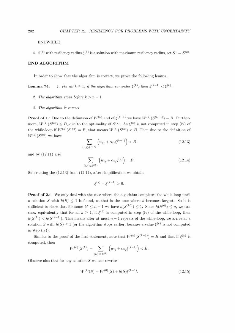
202 CHAPTER 12. RESILIENCY FOR PROBLEMS WITH UNCERTAINTY
ENDWHILE
4. S(k) with resiliency radius ξ(k) is a solution with maximum resiliency radius, set S∗ = S(k).
END ALGORITHM
In order to show that the algorithm is correct, we prove the following lemma.
Lemma 74. 1. For all k ≥ 1, if the algorithm computes ξ(k), then ξ(k−1) < ξ(k).
2. The algorithm stops before k > n− 1.
3. The algorithm is correct.
Proof of 1.: Due to the definition of W (k) and of ξ(k−1) we have W (k)(S(k−1)) = B. Further-
more, W (k)(S(k)) ≤ B, due to the optimality of S(k). As ξ(k) is not computed in step (iv) of
the while-loop if W (k)(S(k)) = B, that means W (k)(S(k)) < B. Then due to the definition of
W (k)(S(k)) we have ∑(i,j)∈S(k)
(wij + αijξ
(k−1))< B (12.13)
and by (12.11) also ∑(i,j)∈S(k)
(wij + αijξ
(k))
= B. (12.14)
Subtracting the (12.13) from (12.14), after simplification we obtain
ξ(k) − ξ(k−1) > 0.
Proof of 2.: We only deal with the case where the algorithm completes the while-loop until
a solution S with h(S) ≤ 1 is found, as that is the case where k becomes largest. So it is
sufficient to show that for some k∗ ≤ n − 1 we have h(S(k∗)) ≤ 1. Since h(S(0)) ≤ n, we can
show equivalently that for all k ≥ 1, if ξ(k) is computed in step (iv) of the while-loop, then
h(S(k)) < h(S(k−1)). This means after at most n − 1 repeats of the while-loop, we arrive at a
solution S with h(S) ≤ 1 (or the algorithm stops earlier, because a value ξ(k) is not computed
in step (iv)).
Similar to the proof of the first statement, note that W (k)(S(k−1)) = B and that if ξ(k) is
computed, then
W (k)(S(k)) =∑
(i,j)∈S(k)
(wij + αijξ
(k−1))< B.
Observe also that for any solution S we can rewrite
W (k)(S) = W (0)(S) + h(S)ξ(k−1). (12.15)

12.2. THE ASSIGNMENT PROBLEM WITH UNCERTAIN COSTS 203
We consider the cases k = 1 and k ≥ 2 separately. For k = 1, since S(0) is an optimal
solution for AP(W (0)), we have W (0)(S(1)) ≥W (0)(S(0)). Also note that
W (0)(S(1)) + h(S(1))ξ(0) = W (1)(S(1)) < W (1)(S(0)) = W (0)(S(0)) + h(S(0))ξ(0),
where the first and last equality are due to (12.15), and the middle inequality is dueW (1)(S(0)) =
B and W (1)(S(1)) < B, as described in the paragraph above. This implies that h(S(1))ξ(0) <
h(S(0))ξ(0) and therefore h(S(1)) < h(S(0)), which is what we want to prove.
So now consider the case k ≥ 2. Recall that S(k−1) is an optimal solution to AP(W (k−1)).
Thus
W (0)(S(k−1)) + h(S(k−1))ξ(k−2) ≤W (0)(S(k)) + h(S(k))ξ(k−2),
but with arguments similar to the proof of the first statement we also have
W (0)(S(k−1)) + h(S(k−1))ξ(k−1) > W (0)(S(k)) + h(S(k))ξ(k−1).
Putting both inequalities together, we obtain
W (0)(S(k−1)) + h(S(k−1))ξ(k−2) −W (0)(S(k))− h(S(k))ξ(k−2)
< W (0)(S(k−1)) + h(S(k−1))ξ(k−1) −W (0)(S(k))− h(S(k))ξ(k−1)
and we simplify to
h(S(k))(ξ(k−1) − ξ(k−2)) < h(S(k−1))(ξ(k−1) − ξ(k−2)).
Since ξ(k−1) > ξ(k−2) by the first statement, this means that h(S(k)) < h(S(k−1)), which finishes
the proof.
Proof of 3.: The algorithm can stop in step 1, step 2, step (iv) in the WHILE-loop and in
step 4.
Clearly, if the algorithm returns a solution S∗ with ξ(S∗) = ∞ obtained in step 1, that
solution has infinite resiliency radius and therefore is optimal. Otherwise, as discussed when
we introduced assignment problem AP(W∞), no B-feasible solution S with h(S) = 0 exists.
If the algorithm stops after step 2 because W (0)(S(0)) > B then no B-feasible exists.
If the algorithm stops in step (iv) of the WHILE-loop, then we have W (k)(S(k)) = B. We
show that in that case, S(k−1) is already a solution of maximum resiliency radius. Since after
checking in step 1 of the algorithm we already know that no B-feasible solution exists which
uses only fixed weights, it is sufficient to show that all solutions, which use at least one uncertain
weight, cannot have a resiliency radius larger than ξ(k−1).
So let S′ be a solution to the assignment problem which uses at least one uncertain weight.

204 CHAPTER 12. RESILIENCY FOR PROBLEMS WITH UNCERTAINTY
As S(k) is an optimal solution to AP(W (k)) and W (k)(S(k)) = B, that means
W (k)(S′) = W (0)(S′) + h(S′)ξ(k−1) ≥ B.
Then, due to h(S′) ≥ 1, for any value ξ′ > ξ(k−1) we have
W (0)(S′) + h(S′)ξ′ > B.
Therefore the resiliency radius of S′ is at most ξ(k−1), which was what we wanted to show.
Finally, assume the algorithm stops in step 4 and returns a solution S∗ = S(k∗) for some
k∗ ≤ n−1. Then we have h(S(k∗)) = 1, due to the exit condition of the while-loop and since no
B-feasible solution S with h(S) = 0 exists (otherwise the algorithm would have stopped after
step 1).
We show that solution S(k∗) with resiliency radius ξ(k∗) is optimal. Note that S(k∗) is
constructed as the optimal solution to assignment problem AP(W (k∗)) with weights
w(k∗)ij = w
(0)ij + αijξ
(k∗−1), 1 ≤ i, j ≤ n.
Towards contradiction, suppose there is a solution S′ with resiliency radius ξ′ > ξ(k∗).
We show that then W (k∗)(S′) < W (k∗)(S(k∗)), in contradiction to the optimality of S(k∗) for
assignment problem AP(W (k∗)).
Using again (12.15), we write
W (k∗)(S′) = W (0)(S′) + h(S′)ξ(k∗−1)
and because h(S(k∗)) = 1, we have
W (k∗)(S(k∗)) = W (0)(S(k∗)) + ξ(k∗−1).
Furthermore, by definition of the resiliency radius we have
W (0)(S′) + h(S′)ξ′ = B = W (0)(S(k∗)) + ξ(k∗).
Together with h(S′) ≥ 1 = h(S(k∗)) and ξ′ > ξ(k∗) > ξ(k∗−1) (the last inequality is due to the

12.2. THE ASSIGNMENT PROBLEM WITH UNCERTAIN COSTS 205
first statement), we obtain
W (k∗)(S′) = W (0)(S′) + h(S′)ξ(k∗−1)
= W (0)(S′) + h(S′)ξ(k∗−1) + h(S′)ξ′ − h(S′)ξ′
= B + h(S′)ξ(k∗−1) − h(S′)ξ′
= B − h(S′)(ξ′ − ξ(k∗−1))
≤ B − (ξ′ − ξ(k∗−1))
< B − (ξ(k∗) − ξ(k∗−1))
= B − ξ(k∗) + ξ(k∗−1)
= W (0)(S(k∗)) + ξ(k∗−1)
= W (k∗)(Sk∗),
in contradiction to the optimality of S(k∗) for problem AP(W (k∗)).
Therefore, solution S′ cannot exist and Sk∗
has maximum resiliency radius ξ(k∗).
Theorem 75. The algorithm is correct and takes at most O(n4) time.
Proof: The correctness is proved to Lemma 74. As the algorithm stops before k > n−1 at most
O(n) assignment problems are solved, each taking at most O(n3) time. Thus the algorithm can
be implemented with a runtime of O(n4).
Note that for the problem with general αij a similar approach could be implemented. How-
ever, it would not lead to a polynomial, but a pseudo-polynomial algorithm. Indeed, in every
step instead of h(S) we reduce the sum of the αij used in solution Sk by at least 1 leading to a
runtime of O(n3Θ), where Θ is the weight of a maximum weight assignment with weight matrix
α = (αij) (recall that for the purposes of finding a most resilient solution we can assume all αij
to be integer).
Norm `q
Again, the arguments from above do not work for general `q-norms, 1 < q < ∞. The problem
here is that with decreasing number h(S) of uncertain weights used in S, the actual deviation
for each uncertain weight has to increase in order to obtain the same radius. Thus the technique
from the last section is not applicable.
The problem may be NP-hard, but we were unable to find a proof for this. Similar to the
more general version with arbitrary fluctuation factors, the question remains open for now.
12.2.3 The bottleneck assignment problem
At the end of our investigation of the assignment problem, we want to compare our findings for
the min-sum version of the assignment problem to the situation for the min-max version of the

206 CHAPTER 12. RESILIENCY FOR PROBLEMS WITH UNCERTAINTY
assignment problem, also known as bottleneck assignment problem. The bottleneck assignment
problem is defined as
AP : min max1≤i,j≤n
wijxij
s.t.n∑i=1
xij = 1, 1 ≤ j ≤ n,n∑j=1
xij = 1, 1 ≤ i ≤ n,
xij ∈ 0, 1, 1 ≤ i ≤ n, 1 ≤ j ≤ n.
Considering uncertainty, let W = (wij) be the estimates for the weights and αij be the
fluctuation factors. Then for a given deviation matrix ∆ = (∆ij), the actual weights are of the
form
w′ij = wij + αij∆ij ,
similar to (12.2).
The bottleneck assignment seems to be much easier to handle than the usual min-sum ver-
sion. We first show that under any norm `q, q ∈ N>0∪∞, worst-case deviations with only one
non-zero entry exist. Then we use this to construct an algorithm to find a most resilient solution
to the bottleneck assignment problem by solving another bottleneck assignment problem.
Lemma 76. Let W and α be the estimated weights and the fluctuation factors for the resiliency
version of the bottleneck assignment problem as above. Let S0 be a given solution and ∆ be any
deviation matrix. Then there exists a deviation matrix ∆, such that
1. ‖∆‖ ≤ ‖∆‖, where ‖ · ‖ may be any `q-norm,
2. f(S0, ∆) = f(S0,∆) and
3. matrix ∆ has only one non-zero entry.
Proof: Given the starting deviation ∆, denote by W ′ = (w′ij) the actual costs, similar to (12.2).
Let (i∗, j∗) ∈ S0 such that w′i∗j∗ = maxw′ij |(i, j) ∈ S0, or equivalently f(S0,W ′) = w′i∗j∗ . If
all entries of ∆, other than ∆i∗j∗ , are 0-entries, then set ∆ = ∆ and we are done.
Otherwise define deviation matrix ∆ by
∆ij =
∆ij , if i = i∗, j = j∗
0, otherwise.
Note that f(S0,W +α∆) = f(S0,W ′) = w′i∗j∗ and that ‖∆‖ ≤ ‖∆‖, by construction. Further-
more, clearly ∆ has at most one non-zero entry, namely ∆i∗j∗ .
Lemma 76 immediately implies that for any solution S0 and any upper bound B a worst-
case deviation with at most one non-zero entry exists. The next lemma deals with computing

12.2. THE ASSIGNMENT PROBLEM WITH UNCERTAIN COSTS 207
that worst-case deviation.
Lemma 77. Let W and α be as in Lemma 76. Let B be a given upper bound and let S0 be a
B-feasible solution. For each (i, j) ∈ S0 let
ξij =
B−wijαij
, if αij > 0,
∞, otherwise.(12.16)
Choose (i∗, j∗) ∈ S0 such that ξi∗j∗ = minξij |(i, j) ∈ S0, with ties broken arbitrarily, and
define deviation matrix ∆ by
∆ij =
ξij , if i = i∗, j = j∗
0, otherwise.
Then ρ(S0,W,B) = ‖∆‖ = ξi∗j∗ and ∆ is a worst-case deviation of S0 under any `q-norm.
Proof: If ‖∆‖ = ∞, i.e. αij = 0 for all (i, j) ∈ S0, then there is nothing to prove. Otherwise,
due to Lemma 76, under any `q-norm, there exists a worst-case deviation with at most one
non-zero entry. Note that amongst all deviations with at most one non-zero entry, ∆ is the one
with the smallest non-zero entry such that the upper bound B is reached. Any further increase
in value ∆i∗j∗ would increase the objective value of solution S0 over bound B, as αi∗j∗ > 0,
and therefore ∆ is a worst-case deviation. The formula for the resiliency radius ρ(S0,W,B)
follows immediately.
From Lemma 77, observe that for any `q-norm, given an upper bound B and a B-feasible
solution S0, we have
ρ(S0,W,B) = ‖∆‖ = ξi∗j∗ = minξij |(i, j) ∈ S0
,
with ξij defined as in (12.16). Thus, a most resilient solution to the bottleneck assignment
problem, is a B-feasible solution S∗, which maximises
min ξij |(i, j) ∈ S∗ .
We construct a new weight matrix Ψ = (ψij), given by
ψij =
ξij , if B − wij ≥ 0,
−1, otherwise.(12.17)
Note that if ψij = −1 for fixed i and j then any solution S with (i, j) ∈ S cannot be B-feasible,
as wij > B.
Using weights Ψ we solve the following maximization version of the bottleneck assignment

208 CHAPTER 12. RESILIENCY FOR PROBLEMS WITH UNCERTAINTY
problem:
AP : max min1≤i,j≤n
ψijxij
s.t.n∑i=1
xij = 1, 1 ≤ j ≤ n,n∑j=1
xij = 1, 1 ≤ i ≤ n,
xij ∈ 0, 1, 1 ≤ i ≤ n, 1 ≤ j ≤ n.
(12.18)
By construction any assignment S with non-negative objective value with respect to problem
(12.18) is also a B-feasible solution with respect to the original problem with weights W , due
to the definition of weights Ψ. Conversely, if S is an assignment with negative objective value
with respect to problem (12.18), then S is not B-feasible with respect to the original problem,
again due to the definition of Ψ.
Let S∗ be an optimal solution to (12.18). If the objective value of S∗ with respect to the new
problem (12.18) is non-negative, then S∗ is a most resilient solution for the resiliency version
with estimated weights W , fluctuation factors α and upper bound B. Otherwise, S∗ is not
B-feasible for the original problem, due to the our observations in the previous paragraph, and
in fact no B-feasible solution exists for the original problem.
Theorem 78. A most resilient solution S∗ for the bottleneck assignment problem with estimated
weights wij, fluctuation factors αij and an upper bound B can be found by solving the bottleneck
assignment problem defined by (12.18) with weight matrix Ψ defined by (12.17).
We can construct matrix Ψ in O(n2) time. After that pre-processing step is done, the
bottleneck assignment problem (12.18) can be solved in O(n2√n log n) time with the algorithm
by [57]. In total, this method to solve the resiliency version of the bottleneck assignment
problem (under any `q norm) takes O(n2√n log n) time.
Interestingly, the result from this section corresponds well to the results for min-max and
min-max regret versions of the bottleneck assignment problem, which also can be solved by
solving the bottleneck assignment problem on a special selected weight matrix. Furthermore,
this method can be generalized to the min-max and min-max regret versions of other bottleneck
combinatorial optimization problems. See [4] and [7] for details. It would be interesting to see
if a generalization of the above approach to the resiliency versions of other bottleneck problems
is also possible.
12.3 Problem 1||∑Cj with uncertain cost
Next we study problem 1||∑Cj . Note that the resiliency version of 1||Cmax is trivial, as
every schedule (without idle times) is a most resilient schedule, similar to the original problem
where every schedule (without idle times) has the same objective value. Also, a worst-case
deviation can always be achieved by increasing only the processing time of the job with the
largest fluctuation factor αj .

12.3. PROBLEM 1||∑CJ WITH UNCERTAIN COST 209
We start by briefly repeating the most important notation and facts. For problem 1||∑Cj
there are given n jobs with processing times pj , 1 ≤ j ≤ n, and the goal is to minimize the total
sum of completion times. It is sufficient to restrict the solution region to all permutations of
jobs, representing schedules without idle times. Consider a schedule S0 given as n pairs (i, j),
1 ≤ i, j ≤ n, indicating assignment of job j to position i. Recall that problem 1||∑Cj can be
modelled as the assignment problem AP with variables
xij =
1, if (i, j) ∈ S0,
0, otherwise,
and costs wij for assigning job j to position i defined as
wij = (n− i+ 1)pj ,
see Section 2.4.4. The input parameters, which now may be subject to uncertainty, are the job
processing times pj .
As in the previous section, we consider first resiliency in its most general type. We discuss the
correspondence between the fluctuation factors of the scheduling problem and the fluctuation
factors of the associated assignment problem. Then we show how to construct worst-case
deviations for the case with arbitrary fluctuation factors αj , using the results from Section
12.2.
After that we turn to the problem of finding most resilient solutions, again first applying
the results from Section 12.2, where possible. Note that similar ideas work for other scheduling
problems in Table 12.1. We also provide a more efficient algorithm than we gave for the
assignment problem, to find a most resilient solution under the `∞-norm. Moreover, given
estimated processing times pj and fluctuation factors αj , the new algorithm allows us to find
the function ρ∞(B), which calculates the optimal resiliency radius dependent on the upper
bound B.
Finally we investigate the version with fluctuation factors αj ∈ 0, 1 and provide an al-
gorithm to find most resilient solutions for norm `1. As for the algorithm for norm `∞, given
estimated processing times pj and fluctuation factors αj , this algorithm is also able to find the
function ρ1(B), which calculates the optimal resiliency radius dependent on the upper bound
B.
12.3.1 The case with arbitrary fluctuation factors αj for the job pro-
cessing times
In the presence of uncertain data, the perturbed job processing times of the form
p′ = p+ α∆

210 CHAPTER 12. RESILIENCY FOR PROBLEMS WITH UNCERTAINTY
result in the following weights for the associated assignment problem:
w′ij = (n− i+ 1) (pj + αj∆j) = wij + (n− i+ 1)αj∆j .
Given fluctuation factors αj for the scheduling problem, the corresponding fluctuation factors
αij for the associated assignment problem are defined by
αij = (n− i+ 1)αj , for 1 ≤ i, j ≤ n. (12.19)
Note that even in the case where all fluctuation factors for αj for the scheduling problem
are equal to 1, for assignment problem we still have fluctuation factors
αij = n− i+ 1, for 1 ≤ i, j ≤ n.
Thus the case with equal fluctuation factors for the scheduling problem translates into a case
with n different fluctuation factors for the assignment problem. This can also happen in other
instances where we transform one problem into another in order to solve it, see for example
the problems in Table 12.1. It is an additional motivation to consider fluctuation factors in the
way we do, as then the factors arising from the transformation of one problem into another can
often be dealt with as part of the fluctuation factors.
Computing radii and worst-case deviations for given solutions
We want to apply the results from Section 12.2.1. In order to do so we deal with fluctuation
factors αij , defined by (12.19), for the weights wij in the associated assignment problem. Fur-
thermore, to make use of the results for the knapsack problem as we did in Section 12.2, we
introduce additional conditions ∆APij = ∆j for 1 ≤ i, j ≤ n, where ∆AP
ij , represent variables in
the knapsack problem KP.
Observe that the worst-case deviations we construct are worst-cases for the scheduling prob-
lem, but not for the associated assignment problem. Indeed, in Section 12.2 we implicitly as-
sume that a worst-case deviation leaves all weights which are not used in the given solution
unchanged. It is easy to check that any deviation, which changes weights not used in a given
solution to the assignment problem is not a worst-case deviation. In contrast to this, if we
change the length of a job j, we also change all weights associated with j in the assignment
matrix, even though only one of those weights is used in any given solution.
In spite of the last observation, we can still use the formulae derived in Section 12.2.1 as
they do not take into account changes happening to the weights not used by a given solution.
As before, we assume that S0 is a B-feasible solution and that αj > 0 for at least one job j.
Note that if αj0 > 0 for a fixed job j0, then αij0 > 0 for all 1 ≤ i ≤ n.
Case `1. Applying (12.4) for an arbitrary solution S0, let (u, v) ∈ S0 be the job-position pair

12.3. PROBLEM 1||∑CJ WITH UNCERTAIN COST 211
such that αuv = maxαij |(i, j) ∈ S0. Then the radius of S0 is
ρ(S0, p, B) =B′
αuv=
B′
(n− u+ 1)αv. (12.20)
A worst-case deviation can be achieved by increasing the length of job v by ρ(S0, p, B),
∆v = B′
(n−u+1)αv,
∆j = 0, for all j 6= v.
Case `q, 1 < q <∞. In order to apply (12.5), first one needs to calculate the constant
Hq =∑
(i,j)∈S0
αq/(q−1)ij =
∑(i,j)∈S0
((n− i+ 1)αj)q/(q−1)
,
Then
ρ(S0, p, B) =B′
H(q−1)/qq
. (12.21)
In order to compute a worst-case deviation, let i [j] be the position of job j in solution
S0, i.e. (i(j), j) ∈ S0 for each job j. Then a worst-case deviation for solution S0 is given
by
∆j =B′
Hq× ((n− i [j] + 1)αj)
1/(q−1), 1 ≤ j ≤ n.
Case `∞. In order to apply (12.7), calculate H∞ =∑
(i,j)∈S0
αij =∑
(i,j)∈S0
((n− i+ 1)αj). Then
the radius is
ρ(S0, p, B) =B′
H∞(12.22)
and a worst-case deviation is given by
∆j = ρ(S0, p, B) =B′
H∞, 1 ≤ j ≤ n.
Going back to the case where all αj are equal, αj = 1, note that in that case the auxiliary
terms Hq and H∞ do not depend on the choice of the given solution. Similarly, the value
αuv = maxαij |(i, j) ∈ S0 used for the `1-norm is defined by the job in the first position,
αuv = n, and equal for all given solutions.
Therefore the radius for any given solution S0 under any `q-norm depends only on the value
B′ = B − f(S0, p). The larger B′ for the given solution, the larger its radius. It is easy to see
that the solution with the largest value B′ is the optimal solution of the original problem. Thus,
in the case where all αj are equal, the optimal solution for the scheduling problem, i.e. the one
with jobs ordered in the SPT-order, is also the most resilient one, similarly to the assignment
problem with equal fluctuation factors. Again this is no longer necessarily the case if the αj

212 CHAPTER 12. RESILIENCY FOR PROBLEMS WITH UNCERTAINTY
are not equal.
Finding most resilient solutions for norms `q, q <∞
For the case of the `1-norm, clearly we can apply the O(n5) time algorithm we developed
for the assignment problem in Section 12.2.1. A better time complexity, using the special
structure of our scheduling problem and its related assignment problem may well be possible.
Below, in Section we discuss such an algorithm for the special case with binary fluctuation
factors, αj ∈ 0, 1. However, for the general case our search for a better algorithm has been
unsuccessful and the question remains open for now.
Similar to the results to the assignment problem, no polynomial time algorithm could be
found for norms `q, 1 < q <∞, and indeed, the time complexity of that problem remains open
as well.
Finding most resilient solutions for norm `∞
Now we consider the `∞-norm, where we can obtain a new positive result, which was not
possible for the assignment problem. Not only can we solve the problem of finding a most
resilient solution for the `∞-norm in O(n2 log n) time, but we can in fact calculate the largest
resiliency radius ρ∞(B) and its corresponding schedule as a function of the upper bound B ≥ 0.
It is sufficient to consider the case where B is large enough such that at least one B-feasible
solution exists, otherwise ρ∞(B) = −1 by definition.
An optimal solution for problem 1||∑Cj is a sequence of jobs given by a known precedence
rule, in this case the SPT-order (shortest processing time first). Note that it is observed, e.g.
in [70], that an optimal schedule for problem 1||∑Cj stays optimal under perturbation of the
processing times, if and only if the SPT-order of jobs does not change. Recall also that due
to Statement 68, for a given solution S0 and a given upper bound B there exists a worst-case
deviation ∆, such that all entries in ∆ are equal. So we can restrict our consideration to
deviations ∆ with ∆j = ξ for all j. In that case we have actual processing times
p′j = pj + αjξ.
Using these two properties, we show how to identify O(n2) candidate schedules for most resilient
solutions and then compute the function ρ∞(B) as the upper envelope of O(n2) lines arising
from those candidate schedules.
We first show that starting with ξ = 0 and increasing it continuously, the SPT-order of the
actual processing times p′j changes at most O(n2) times. Let S0 be the SPT-schedule for the
original processing time estimates pj and let jobs be numbered in the order in which they appear
in S0. Furthermore let B(0) be the objective value of schedule S0 for the original processing
time estimates pj . It is easy to see that we can additionally assume that in S0 ties between the
pj are, where possible, broken by scheduling first the job with the smaller αj value. Then there

12.3. PROBLEM 1||∑CJ WITH UNCERTAIN COST 213
is some fixed value ξ for which two given jobs j1 < j2 change their SPT-ordering for the actual
processing times p′j if and only if pj1 < pj2 and αj1 > αj2 . At value ξ the processing times of
jobs j1 and j2 are equal, i.e.
pj1 + αj1 ξ = pj2 + αj2 ξ
or
ξ =pj2 − pj1αj1 − αj2
.
Since αj1 > αj2 the quotient is always well-defined and since pj1 < pj2 we have ξ > 0, i.e.
the order does not change for very small values ξ. Observe that without breaking ties in the
ordering of the pj as described above above, we only get conditions pj1 ≤ pj2 and αj1 > αj2
and ξ = 0 is possible.
Conditions pj1 < pj2 and αj1 > αj2 imply that there are at most n such changes for each job,
leading to a total of at most n2 changes in the overall SPT-ordering as ξ increases. These O(n2)
different SPT-orderings for the actual processing times p′j depending on ξ are the previously
mentioned candidate schedules.
In order to compute those schedules, we first compute the O(n2) values of ξ at which changes
to the order of the actual processing times happen. For two jobs j1 < j2 with pj1 < pj2 and
αj1 > αj2 let
ξ(j1,j2) =pj2 − pj1αj1 − αj2
.
We re-order the values ξ(j1,j2) in non-decreasing order, obtaining a sequence ξ(1), ξ(2), . . . , ξ(κ),
for some integer κ ≤ n2. In order to make the following arguments easier, we assume that the
values ξ(ι) are pairwise different from each other. At the end of the section we will discuss what
happens if this is not the case and show that the same results still apply.
Denote by Sι the SPT-schedule for the actual processing times p(ι)j = pj+αjξ
(ι). Again, ties
in the ordering of the actual processing times should be broken, where possible, by scheduling
first the job with the smaller αj value. Then clearly Sι is an SPT-schedule for all values of
actual processing times p′j = pj + αjξ, with ξ(ι) ≤ ξ < ξ(ι+1).
Note that when transforming schedule Sι into Sι+1 only two jobs swap their position,
because the values ξ(ι) are pairwise different. Moreover, these two jobs are neighboring jobs,
since otherwise another job would swap positions with at least one of them, which again cannot
happen because the ξ(ι) are pairwise different. Therefore knowing Sι, the schedule Sι+1 can be
obtained in O(1) time.
For each schedule Sι we also compute value B(ι) as the objective value of schedule Sι
assuming the processing times are p(ι)j = pj + αjξ
(ι). Note that for a given schedule Sι its
objective value increases linearly in ξ with the factor
λ(ι) =
n∑j=1
((n− ij(Sι) + 1)αj) ,

214 CHAPTER 12. RESILIENCY FOR PROBLEMS WITH UNCERTAINTY
where ij(Sι) is the position of job j in Sι. Observe that the change from λ(ι) to λ(ι+1) can
again be computed in O(1), as only the position of two neighboring jobs is swapped. If job j1
and j2 with pj1 < pj2 swap positions from schedule Sι to schedule Sι+1 then
λ(ι+1) = λ(ι) + αj2 − αj1 .
Then we can compute
B(ι+1) = B(ι) + λ(ι)(ξ(ι+1) − ξ(ι)).
As the values ξ(ι) are pairwise different, the same is true for the values B(ι).
In order to save space and time, it is sufficient to only commit the values ξ(ι), B(ι) and
λ(ι) to memory. Each schedule Sι can be found in O(n log n) time for a given deviation ξ, if
necessary.
Lemma 79. We can compute values ξ(ι), B(ι) and λ(ι) in O(n2 log n) time.
Proof: Clearly computing values ξ(ι) takes at most O(n2) time and subsequent sorting for n2
values takes O(n2 log n) time.
After finding schedule S0 in O(n log n) time and value B(0) in O(n) time as pre-processing
steps, we can recursively obtain the schedules Sι. Note that we do not produce schedules Sι,
instead we obtain Sι by manipulation of the already existing sequence in O(1) time for each
ι. Then, for schedule Sι we compute and save the values B(ι) and λ(ι) again in O(1) time.
As there are O(n2) different schedules, the process of computing all values B(ι) and λ(ι) takes
O(n2) time.
The total processing time is dominated by sorting the values ξ(ι), which takes O(n2 log n)
time.
Note that if schedules Sι are all saved separately, then O(n2) permutations of n numbers
have to be saved, which takes at least O(n3) time and space.
We now show that we actually chose the right set of candidate schedules, i.e. that given any
upper bound B there is ι ∈ 0, 1, 2, . . . , κ such that Sι is a most resilient solution for bound
B. Note that we can again assume B ≥ B0, such that some B-feasible solution exists.
Lemma 80. Let an upper bound B ≥ B0 be given and choose ι such that B(ι) ≤ B < B(ι+1)
or ι = κ if B ≥ B(κ). Then Sι is a most resilient solution for the upper bound B.
Proof: Let ξ = ρ(Sι, p, B) be the resiliency radius of Sι for the upper bound B. Clearly, we
have ξ(ι) ≤ ξ < ξ(ι+1) or ξ ≥ ξ(κ) if ι = κ, by definition of B(ι). Assume there is a solution S∗
with a larger resiliency radius ξ.
Without loss of generality we can assume that not all αj are 0 (otherwise there is no
uncertainty). For a solution S let F (S) be the objective value of S assuming the processing
times are pj = pj + αj ξ and define F (S) analogously. Then
F (S∗) < F (S∗) = B = F (Sι),

12.3. PROBLEM 1||∑CJ WITH UNCERTAIN COST 215
a contradiction, as Sι is, by definition, an optimal schedule for processing times pj = pj + αj ξ,
namely the one with jobs in SPT-order.
We can now calculate the function ρ∞(B), the maximum resiliency radius dependent on
B, as the piecewise linear function given by the points (B(ι), ξ(ι)) with the slope 1λ(ι) between
points ((B(ι), ξ(ι)) and (B(ι+1), ξ(ι+1)). It can be viewed as the upper envelope of the O(n2)
lines given by the formulas
ξ(ι) −B(ι) 1
λ(ι)+
1
λ(ι)B.
The algorithm by [149] computes the upper envelope of k lines in O(k log k) time, leading to a
total complexity of O(n2 log n) time to compute function ρ∞(B).
Theorem 81. The function ρ∞(B) which for every upper bound B calculates the maximum
resiliency radius under the `∞-norm can be computed in O(n2 log n) time as the upper envelope
of O(n2) lines.
Now return back to our assumption that the values ξ(ι) are pairwise different. Note that
some of the O(1) computations will take more time if there are equalities amongst the ξ(ι), as
several computations have to be done in the same step. However, if there are k equal values
ξ(ι), ξ(ι+1), . . . , ξ(ι+k−1), then then computing the new schedule Sι = Sι+1 = . . . Sι+k−1 and
the values B(ι) = B(ι+1) = . . . = B(ι+k−1) still only involves inverting the order of O(k) jobs,
which can be done in O(k) time. The total time taken to compute all schedules (or respectively
all values B(ι)) is still bounded by the number of values ξ(ι), which is bounded by O(n2). Thus
the complexity analysis from above still holds.
The basic ideas presented in this section on how to obtain a set of candidate schedules for the
most resilient solution also work for other sequencing problems with known precedence rules,
such as EDD (earliest due date first) for the maximum lateness objective, Smith’s rule for the
weighted total sum of completion times or Johnson’s rule for problem F2||Cmax. However, note
that the time analysis might differ for other problems and we might not necessarily be able to
obtain the function ρ∞(B) as easily as we did here.
12.3.2 The case with binary fluctuation factors αj ∈ 0, 1
In this section we show that if fluctuation factors are restricted to αj ∈ 0, 1 then we can
calculate the largest resiliency radius ρ1(B) under the `1-norm as the function of the bound
B. Similar to the result of Theorem 81 the function ρ1 is a piecewise linear function, given as
the upper envelope of a set lines. Again, those lines are given by candidate schedules, this time
O(n) many, rather than O(n2).
Recall that in the case where fluctuation factors are restricted to the values 0 and 1, a job
j is called uncertain if αj = 1 and job j is called fixed if αj = 0. Let J ′ = j′1, j′2, . . . , j′ν and
J ′′ =j′′1 , j
′′2 , . . . , j
′′µ
be the subsets of uncertain and fixed jobs respectively, J = J ′ ∪ J ′′,

216 CHAPTER 12. RESILIENCY FOR PROBLEMS WITH UNCERTAINTY
with the jobs in each set numbered in the SPT order:
pj′1 ≤ pj′2 ≤ · · · ≤ pj′ν ,pj′′1 ≤ pj′′2 ≤ · · · ≤ pj′′µ .
We assume that neither of the two sets are empty. Otherwise, if set J ′ is empty, all jobs are
fixed and we are left with the traditional scheduling problem. If set J ′′ is empty, then all jobs
have fluctuation factor 1 and the most resilient solution (for any B) is the solution where jobs
are in order of non-decreasing processing time estimates pj . Furthermore, we assume that B
is large enough such that a B-feasible solution exists. Otherwise the largest resiliency radius is
−1 by definition.
Due to formula (12.20) and since αj ∈ 0, 1, for any B-feasible schedule S there exists
a worst case deviation ∆ where only the processing time of the earliest uncertain job in S is
increased. If the earliest uncertain job in S is at position i, then the resiliency radius of S is
given by
ρ1(S, p,B) =B′
n− i+ 1=B −∑Cj(S)
n− i+ 1. (12.23)
Thus it only depends on the objective value of schedule S and the position of the earliest
uncertain job. It decreases, as the objective value increases, but increases, as the position of
the earliest late job increases. Consequently, we obtain the following lemma.
Lemma 82. In any B-feasible schedule S∗ with the largest resiliency radius, the jobs from J ′,if considered in isolation from J ′′, appear in the non-decreasing order of pj. The analogous
statement holds for the jobs from J ′′.
Proof: Suppose S is a schedule for which the statement of the lemma does not hold. Construct
schedule S′ where jobs in J ′ take up the same positions as in S but are in SPT order. Clearly,
the objective value of S′ is smaller than that of S, thus if S is B-feasible, then so is S′.
Furthermore the position of the earliest uncertain job in S′ is the same as in S, since the job
sets J ′, and J ′′ occupy the same positions in the schedule as before. Therefore, by (12.23),
the resiliency radius of S′ is larger than that of S, and S cannot be a most resilient solution.
Analogously, we proof the same statement for J ′′.
Similar to Lemma 82 we can prove the next lemma.
Lemma 83. Let S∗ be a B-feasible schedule with the largest resiliency radius, and let i be the
position of the earliest uncertain job in S∗. Then the jobs in positions 1, 2, . . . , i− 1 considered
independently are in SPT-order. Similarly, the jobs in positions i + 1, i + 2, . . . , n considered
independently are in SPT order.
Proof: The first statement is clear, as all jobs in positions 1, 2, . . . , i− 1 are fixed, due to the
definition of i, and therefore in SPT order by Lemma 82.

12.3. PROBLEM 1||∑CJ WITH UNCERTAIN COST 217
Suppose the second statement does not hold and the jobs in positions i + 1, i + 2, . . . , n
considered independently are not in SPT order. Then consider schedule S where the same set
of jobs occupies positions i+ 1, i+ 2, . . . , n as in S∗, but they are in SPT order. Similar to the
proof of Lemma 82 the objective value of schedule S is smaller than that of schedule S∗ and
the position of the earliest uncertain job remains the same. Therefore, by (12.23), schedule S
has a larger resiliency radius than schedule S∗, in contradiction to the assumption that S∗ is a
schedule with the largest resiliency radius.
From Lemmas 82 and 83 the structure of a candidate schedule for the most resilient schedule
is given uniquely by the position of the first uncertain job. Since the latest possible position
for the first uncertain job is µ+ 1, if all µ fixed jobs are at the start of the schedule, there are
µ+ 1 ≤ n candidate schedules.
Theorem 84. For norm `1, the candidate schedule S(i) where the earliest uncertain job is in
position i, 1 ≤ i ≤ µ+ 1, is of the form:
– fixed jobs j′′1 , j′′2 , . . . , j
′′i−1 ∈ J ′′ are scheduled in SPT order in positions 1, 2, . . . , i− 1,
– the shortest uncertain job j′1 is inserted in position i,
– the remaining jobs j′2, j′3, . . . , j′ν∪j′′i , j′′i+1, . . . , j′′µ, certain and uncertain, are scheduled
in SPT order in positions i+ 1, i+ 2, . . . , n.
Proof: The theorem follows immediately from Lemmas 82 and 83.
Therefore, for norm `1, there are at most n different job sequences S(1), S(2), . . . , S(µ+1),
each of which corresponds to a certain insertion position of j′1. In fact, with the same arguments
we used in the proofs of the two lemmas we can see that there is no point in inserting job j′1before its place in the overall SPT order, as it does not lead to a most resilient schedule.
Therefore, assuming jobs are numbered in order of non-decreasing processing times, we only
need to consider insertion positions i with j′1 ≤ i ≤ µ + 1 and the corresponding schedules
S(j′1), S(j′1+1), . . . , S(µ+1).
For schedule S(i), given a vector p of fixed processing time estimates, the function ρ1(S(i), p, B)
is a linear function given by
ρ1(S(i), p, B) = −∑Cj(S
(i))
n− i+ 1+
1
n− i+ 1B,
if B ≥∑Cj(S(i)). Define for all B ≥ 0 the linear function
ρS(i)(B) = −∑Cj(S
(i))
n− i+ 1+
1
n− i+ 1B,
the linear extension of ρ1(S(i), p, B).
Lemma 85. The set of functions ρS(i)(B) for all schedules S(i) can be computed in O(n) time.

218 CHAPTER 12. RESILIENCY FOR PROBLEMS WITH UNCERTAINTY
Proof: Since function ρS(i)(B) is given by the position index i and objective value∑Cj(S
(i)),
it is sufficient to show that all objective values∑Cj(S
(i)) can be computed in O(n) time.
Note that schedule S(j′1) can be computed in O(n log n) time and∑Cj(S
(j′1)) can be com-
puted in O(n) time. Schedule S(i+1) can be obtained from schedule S(i) by moving the i-th
fixed job j′′i from position j′′i to position i. All jobs between position i and j′′i − 1, which are
the first j′′i − i uncertain jobs jobs j′1, j′2, . . . , j
′j′′i −i, are moved one position to the back of the
schedule.
Therefore, we can recursively obtain objective value∑Cj(S
(i+1)) from∑Cj(S
(i)) using
∑Cj(S
(i+1)) =∑
Cj(S(i)) + (n− i+ 1− (n− j′′i + 1))pj′′i −
ji′′−i∑k=1
pj′k .
If in each step we remember the current value of the term
ji′′−i∑k=1
pj′k ,
then each uncertain job only needs to be added once to the term, while computing the objective
value of all schedules S(i). Furthermore each fixed job is moved at most once while computing
the objective value for all schedules S(i). Therefore, recursively computing the objective values
for all schedules S(i) takes at most O(µ+ ν) = O(n) time.
The complete function ρ1(B), which for any given B such that at least one B-feasible
solution exists, calculates the maximum resiliency radius, is then given by the upper envelope
of the O(n) lines ρS(i)(B). If no B-feasible solution exists, the maximum resiliency radius is
−1. Since the upper envelope of k functions can be found in O(k log k) time by the algorithm
due to [149], the problem of computing ρ1(B) is solvable in O(n log n) time.
We summarize the main results of this section in the theorem below.
Theorem 86. If fluctuation factors αj are restricted to αj ∈ 0, 1, then the resiliency version
of problem 1||∑Cj under the `1-norm is solvable in O(n log n) time.
Furthermore, the function ρ1(B) which, for given processing time estimates p, calculates the
maximum resiliency radius under the `1-norm as a function of the bound B can be computed in
O(n log n) time, as the upper envelope of O(n) lines.
12.3.3 Problem P ||∑Cj
Note that in order to generalise the results from Sections 12.3.1 and 12.3.2 to the problem
with m machines, we have to adjust the positional factors in the definition of the associated
assignment problem. Instead of wij = (n− i+ 1)pj we define
wij =
⌈n− i+ 1
m
⌉pj .

12.3. PROBLEM 1||∑CJ WITH UNCERTAIN COST 219
Consequently, in the definitions for the version with uncertainty, with fluctuation factors for αj
for processing time estimates pj and a given deviation ∆, the actual weights are
w′ij =
⌈n− i+ 1
m
⌉(pj + αj∆j)
=
⌈n− i+ 1
m
⌉pj +
⌈n− i+ 1
m
⌉αj∆j
= wij +
⌈n− i+ 1
m
⌉αj∆j .
Thus, we define the fluctuation factors for the associated assignment problem as
αij =
⌈n− i+ 1
m
⌉αj .
Note that problem P ||∑Cj can still be treated as a sequencing problem, using the following
transformation from a sequence of jobs to a schedule. Given a sequence of jobs φ, suppose the
position of job j is φ(j) = km + r for 1 ≤ r ≤ m. Then we schedule job j as the k + 1-st job
on machine r. The transformation from a schedule back to a sequences is done analogously.
In that case, scheduling jobs in the SPT-order is still an optimal solution for the traditional
problem.
It is easy to see that the same arguments as in Sections 12.3.1 and 12.3.2. work to generalise
the results from those sections.

220 CHAPTER 12. RESILIENCY FOR PROBLEMS WITH UNCERTAINTY

Chapter 13
Conclusions and Further research
In this chapter we present conclusions and suggest some directions for future research. We also
point out some challenges that have not been mentioned explicitly before. Since open questions
for the specific problems we investigated have already been pointed out in the appropriate
sections of Chapter 12, we do not repeat them here. Instead, most of our remarks are either
about generalization of the obtained results or general insights in the new concept of resiliency.
Conclusions about resiliency in general and some challenges are discussed in Section 13.1.
In Section 13.2 we deal with the possibility of generalizing some of our results, especially for
scheduling. Finally, Section 13.3 is about some broader ideas for possible future research.
13.1 Advantages and challenges of the resiliency concept
Our general results and the two problems we studied more closely indicate strongly that re-
siliency is a viable concept for the measurement of solution quality under uncertainty. Note
that resiliency allows to measure the quality of any given solution via the resiliency radius,
as well as algorithmic search for a “best” solution via the concept of most resilient solutions.
In this way, resiliency lies in between stability analysis and robust discrete optimization, with
connections to both of these concepts. Considering mostly the `1 and `∞-norm, we achieved
positive results for both problems we considered, computing the resiliency radius of a given
solution and finding most resilient solutions.
Compared to stability, the resiliency radius for the two problems under investigation is
no harder to compute than the stability radius of a solution. This remains true, even if we
allow for different input parameters to have different scale of uncertainty, i.e. for arbitrary
fluctuation factors. Additionally, we can compute the resiliency radius of any given solution
S0, not necessarily optimal or ε-optimal. Furthermore, it appears that the resiliency radius
221

222 CHAPTER 13. CONCLUSIONS AND FURTHER RESEARCH
may well be computable in a similar manner for problems that are not polynomially solvable
(how to do so for the TSP problem was explained in Section 12.2.1). As we pointed out in
Section 11.2, usually computing the stability radius of a solution is at least as hard as solving
the original problem [125, 148].
Compared to robustness, our examples suggest that positive complexity results seem very
much possible for the resiliency versions of polynomially solvable combinatorial optimization
problems. Recall that for robustness many problems other than interval min-max versions seem
to be computationally hard [4].
However, there are also several challenges. We detail two possible disadvantages of resiliency
here. The first is the question of practical application. While we have given good theoretical
indication that resiliency is a useful concept, and it appears easy to apply in practice, the
practical usefulness remains to be seen. The applications for stability and sensitivity analysis
(see, e.g. [142]), are helpful to see some practical use for resiliency radii, but especially the
practical interest of a most resilient solution has yet to be studied.
One facet of this, which resiliency has in common with stability and robustness, is the
reliance on worst case deviations/scenarios in order to determine the quality of a solution. For
resiliency worst case deviations often take very specific forms, where all entries in the deviation
vector are equal, or a deviation vector has only one non-zero entry.
In many practical applications this is questionable, as the worst case deviation/scenario
might only happen with a very low probability, as has been observed for robustness in [4].
There are several possible solutions mentioned in [4], which may help to refine the definition of
resiliency to become more practical. In Section 13.3 we suggest several ideas how to deal with
this issue.
Another challenge arises because the definition of resiliency implicitly assumes that a solu-
tion S for input parameters η still “makes sense” for the perturbed input parameters η + ∆.
This assumption is appropriate for the assignment problem and similar problems, where solu-
tions can be represented as vectors x with 0/1-entries, the input parameters are weights and the
objective function is of the form∑nj=1 ηjxj or maxnj=1 ηjxj . It is also appropriate for scheduling
problems where a schedule is uniquely specified by a sequence of jobs on each machine, such as
problems 1||f with f a traditional scheduling objective or F2||Cmax.
On the other hand it is unclear how to handle more complicated problems, where a solution
cannot be represented in a simple combinatorial structure. In scheduling, for example, preemp-
tion represents such a challenge. If the length of an operation increases due to perturbation, it
is unclear which piece of the operation, if preempted, should be lengthened. Another example
are scheduling objectives with an earliness component, where an optimal schedule may have
idle times and a simple representation as a sequence of jobs is no longer sufficient. Here, as the
processing time of an operation becomes longer, it may be unclear if the additional processing
load should be scheduled in front of the original operation (if there is idle time somewhere in
front of the operation) or after the original operation (pushing other operations back) or both.

13.2. GENERALIZATIONS TO OTHER PROBLEMS 223
If problems of such a type should be considered in the future, either the definition of re-
siliency has to be refined, or these and possibly other questions need to be part of the research.
For example, in the case of preemption it may be appropriate in an applied scenario to declare
rules on which job pieces to change in case of deviation from the predicted processing time
values. Different rules may lead to different resiliency radii and the search for a best set of rules
may be an interesting challenge.
It may also happen for some problems that the solution S simply becomes infeasible for the
perturbed input data, i.e. is no longer part of the solution set. However, this is less of an issue,
since we can simply define the weight of an infeasible solution to be equal to ∞ and thus still
measure the resiliency radius of S.
All in all, despite these two and more challenges that might emerge along the way, we believe
that resiliency is an exciting and useful concept for further study. It lies in between two very
well established concepts in combinatorial optimization and unites advantages of both areas.
We believe there is the potential for many interesting results.
13.2 Generalization and transfer of our results to other
problems
We consider first possible extensions of the results for the assignment problem to general 0− 1
combinatorial optimization problems (defined below). After that we turn to extensions of the
additional results obtained for problem 1||∑Cj that are not reliant on those for the assignment
problem.
13.2.1 Resiliency for 0− 1 combinatorial optimization problems
It was mentioned previously that the assignment problem is a special case of a combinatorial
optimization problem where the input parameters ηj are weights, a solution can be represented
as a vector x with 0/1-entries and the objective is to minimize a function f =∑nj=1 ηjxj . These
problems are often times referred to as 0 − 1 combinatorial optimization problems, see, e.g.,
[4, 28].
Many well-known and important problems can be described in that way, such as shortest
path, minimum spanning tree and minimum weight perfect matching on a given fixed graph G.
It seems very likely that the results we achieved for the assignment problem, both for computing
resiliency radii and for finding most resilient solutions, can be generalized to all problems of
this type, or at least a subclass.
I order to compute resiliency radii for 0 − 1 combinatorial optimization problems, note
that we can reproduce formulation KP that was used to compute a worst case deviation for
the assignment problem (see Section 12.2.1). Given a solution vector x0 define solution S0 =
j|xj = 1, similar to the notation for the assignment problem. Then a worst case deviation of

224 CHAPTER 13. CONCLUSIONS AND FURTHER RESEARCH
S0 can be computed by formulation
KP∗: min∑j∈S0
(∆j)q
s.t.∑j∈S0
αj∆j ≥ B′,
∆j ≥ 0, j = 1, 2, . . . , n.
Again B′ is given by the difference of the given bound B and the original objective value of the
solution given by vector x, i.e. B′ = B −∑j∈S0 ηjxj .
The result from Lemma 69 can be extended as well. Thus, it should be possible to derive
formulas of a similar type as we did for the assignment problem.
For finding most resilient solutions, at least the result from Theorem 71 appears general-
izable. Using a similar approach, we solve the original problem O(n) times, where n is the
number of input parameters. This way, we obtain O(n) candidate solutions and pick the one
with the largest resiliency radius. The total process takes O(nT (n)) time, where T (n) is the
time it takes to solve the original problem. Note that for the assignment problem we used
the usual notation of a weight matrix (rather than a vector with n2 entries) and therefore the
number of input parameters is n2.
Details for the generalization of these and other results still have to be worked out. Similarly,
it would be interesting to see if the approach used for the bottleneck assignment problem can
be generalized to the bottleneck version of a general 0− 1 combinatorial optimization problem,
where the objective is to minimize function maxnj=1 ηjxj instead of∑nj=1 ηjxj .
13.2.2 Resiliency for list scheduling problems
In sections 12.3.1 and 12.3.2 we obtain results for the resiliency version of problem 1||∑Cj ,
based on the knowledge that an optimal schedule is given by the SPT-order. A scheduling
problem which can be solved by sequencing jobs in a known way is sometimes called a list
scheduling problem, see, e.g., [70]. Prominent examples are problems 1||Lmax, 1||∑wjCj and
F2||Cmax.
We solve the resiliency version of problem 1||∑Cj under the `∞ norm by obtaining O(n2)
candidate schedules, one for each time the SPT-order changes. Then for a given bound B we
pick the most resilient of these O(n2) schedules.
A similar approach should work to find most resilient solutions for other list scheduling
problems. For example we would obtain one candidate schedule for each possible order of due
dates for problem 1||Lmax. Again, details have to be worked out, but seem rather straight
forward.
However, finding the function ρ∞(B) (see Theorem 81) for an arbitrary list scheduling
problem can be more tricky. Note that for different objective functions the schedules do not
necessarily give rise to a linear function, as they did for problem 1||∑Cj . Indeed, for problem

13.2. GENERALIZATIONS TO OTHER PROBLEMS 225
1||Lmax the function is may only be piecewise linear as the objective value of a given schedule
stays the same for certain deviations (if only one job is very late, small changes for other jobs
do not affect the maximum lateness). This issue has to be investigated further.
It is also unclear how to compute the resiliency radius for any given list scheduling problem.
The method from the assignment problem we used to solve this issue for problem 1||∑Cj
cannot be immediately extended to other list scheduling problems. Note that neither 1||Lmax
nor 1||∑wjCj can be modelled as the assignment problem.
13.2.3 Resiliency for other scheduling problems
Naturally, it would also be interesting to see which of our results, if any, extend to other
scheduling problems, not necessarily of list scheduling type. Most interesting amongst those
might be problem 1||∑Uj , the first general single machine problem not of list scheduling type,
and O2||Cmax, which is prominently featured in other parts of this thesis. Note however, that
computing resiliency radii might also be of interest and solvable for NP-hard single machine
problems 1||∑Tj , 1||∑wjTj and 1||∑wjUj .
Unfortunately none of the results we achieved seem easily generalizable to other scheduling
problems, not of list scheduling type. For problem O2||Cmax the resiliency radius of a given
schedule may be easily computable for norm `1, where it seems likely that the length of only
one operation needs to be increased for a worst case deviation. It might be sufficient to increase
on each machine the length of the operation with the largest fluctuation factor and then pick
whichever of the two deviations leads to a violation of the bound B earlier. This approach seems
to work for schedules without idle times (other than in the end of the schedule). Schedules with
idle times are most likely more problematic. Note that idle times in the middle of the schedule
may arise in spite of the objective being regular.
For problem 1||∑Uj and the `1-norm the situation seems to be more complicated. It is
easy to come up with examples where more than one processing time or due date has to be
changed in a worst case deviation. Indeed, consider the example with two jobs and input data
j pj α(p)j dj α
(d)j
1 2 1 3 0
2 2 3 8 0
,
where α(p)j is the fluctuation factor of the processing time of job j and α
(d)j is the fluctuation
factor for the due date of job j. Consider solution S0 with job sequence (1, 2) and upper bound
B = 1 on the objective. Due to the piecewise constant objective function, when the upper
bound B is reached there is still some leeway for deviation before it is violated.
In order to violate bound B both jobs have to be late. Clearly, the only way for job 1 to be
late is to increase its processing time by 1. However, for the second job it is better to increase
its own processing time, due to the larger fluctuation factor. Thus, in a worst case deviation,

226 CHAPTER 13. CONCLUSIONS AND FURTHER RESEARCH
both processing times need to be increased. Similarly, note that if only due dates are subject to
uncertainty, then clearly both due dates need to be decreased in order to make both jobs late.
Turning to norm `∞, recall that all entries in a worst case deviation vector are equal for
problem O2||Cmax due Statement 68. For problem 1||∑Uj , it is easy to generalize Statement
68 in order to see that the entries in the deviation vector are of equal absolute value, positive
for the processing times and negative for the due dates. For both problems, 1||∑Uj and
O2||Cmax, a way to compute the resiliency radius of a given schedule may be found by careful
analysis of such deviations vectors. Here, it needs to be investigated how the value of a solution
changes when all processing times increase simultaneously (and for 1||∑Uj due dates decrease
simultaneously).
13.3 Future research – a broader view
In this section we suggest some directions for further research that are not directly related to
the results we achieved previously. We focus on two areas, one an extension of the definition
for resiliency in order to deal with some of the challenges discussed in Section 13.1, the other
deals with the application of resiliency to linear programming.
13.3.1 Interval based resiliency
As was observed in Section 13.1, one major drawback of the resiliency concept is the reliance
on worst case deviations which may not be very likely to happen. One way of dealing with this
problem is to give not only an estimate ηj and a fluctuation factor αj for each input parameter,
but also an interval of likely deviations Ij =[ηj, ηj
], similar to the definitions in interval min-
max and min-max regret problems [4]. Then all entries ∆j in the deviation vector must be such
that ηj + αj∆j ∈ Ij . Clearly, this means
∆j ∈[η
j− ηjαj
,ηj − ηjαj
].
The intervals may be chosen such that no deviations outside of the intervals are possible.
If a certain amount of risk is acceptable, the intervals can also be chosen tighter, such that
deviations outside the interval are possible, but only with a small chance.
Observe that for the results we achieved up until now, it is necessary that the deviation
vector is not restricted in such a way. For small values of bound B many results may still hold,
as the deviations do not become very large, however, for larger values of B this is no longer
true. What is more, it is no longer the case that for the `1-norm it is often sufficient to consider
deviations with only one non-zero entry, since the allowed range of deviation may not be large
enough.
Similarly, for the `∞ norm, not all entries in a deviation vector are equal. However, State-
ment 68 appears to be generalizable in the following way. Given a largest deviation ξ, a worst

13.3. FUTURE RESEARCH – A BROADER VIEW 227
case deviation vector is of the form ∆j = minξ,∆j for objective functions non-decreasing in
the input parameters, where
∆j =ηj − ηjαj
.
Generalizations for objective function non-increasing in the input parameters are possible in an
analogous way.
In order to compute resiliency radii for the `∞-norm and an objective function non-decreasing
in the input parameters, it may be possible to proceed in the following way. First, increase all
entries of the deviation vector to the smallest value ∆j . If upper bound B is violated, then a
worst case deviation can be computed ignoring the intervals. Otherwise, continue and increase
all entries in the deviation vector that still can be increased to the next smallest value ∆j . Those
which cannot be increased are fixed at the previous value ∆j . Again, test if the upper bound
B is violated. If yes, compute a worst case deviation with some values fixed at the smallest ∆j
and all other entries of the deviation vector all equal to some ξ between the smallest and the
second smallest value of ∆j . If the upper bound B is still not violated, continue in the same
way.
Such an approach should work for the assignment problem with arbitrary fluctuation factors
and thus also for the associated scheduling problems. For the assignment problem this suggests
that O(n log n) time is needed to compute the resiliency radius, due to the sorting of values ∆j .
More careful analysis is needed to verify this result.
For other problems computing the resiliency radius may not be as straight forward, depend-
ing on how difficult it is to compute the resiliency radius under the `∞-norm without additional
intervals.
13.3.2 Resiliency for linear programming
A lot of research in stability and sensitivity has been done for linear and integer linear program-
ming, see, e.g., [66]. Robust mathematical programming, which in the definition of scenarios
is very similar to robust combinatorial optimization as we introduced above, is also an impor-
tant and prolific, albeit more recent field [14]. It seems natural to consider resiliency for linear
programming as well.
Consider a linear program
min cx
s.t. Ax ≥ b,
x ≥ 0,
for a constraint matrix A, a cost vector c and a right-hand side b. In order to be able to deal
with infeasible solutions, define the objective value of an infeasible solution to be equal to ∞.
Given a bound B <∞ this means that infeasible solutions are not B-feasible.
We first deal with the case where only the cost vector c is subject to uncertainty. Given
fluctuation factors αj for cost component cj , upper bound B and a B-feasible solution x0, we

228 CHAPTER 13. CONCLUSIONS AND FURTHER RESEARCH
can compute a worst case deviation of x0 under the `q-norm via formulation
F0 : min∑nj=1 ∆q
j
s.t.∑nj=1
((αjx
0j )∆j
)≥ B′,
∆j ≥ 0.
Here, similar to formulation KP from Section 12.2.1, B′ = B −∑nj=1 cjx
0j . Note that due to
x0j ≥ 0 by definition of the original linear program, we can assume ∆j ≥ 0 without loss of
generality. This also means that for norm `∞ again a worst case deviation exists where all
entries in the deviation vector are equal. Defining new fluctuation factors α′j = αjx0j we should
be able to adjust the formulas from Section 12.2.1 in order to compute the worst case deviation
and resiliency radius of solution x0.
Finding a most resilient solution on the other hand is not as straight forward. An approach
similar to the one in Section 12.2.1 for the `1-norm does not seem promising, as the xj are
continuous variables, rather than boolean. Currently we do not know what approaches may be
promising.
Now consider the case where the constraint matrix A = (aij) and the right-hand side b
may be uncertain. Assume there are m constraints, i.e. A ∈ Rm×n, and let αij , i = 1, . . . ,m,
j = 1, . . . , n+ 1, be the fluctuation factors such that the actual values of the parameters given
deviations ∆ij , i = 1, . . . ,m, j = 1, . . . , n, are
a′ij = aij + αij∆ij , i = 1, . . . ,m, j = 1, . . . , n,
b′i = bi + αi(n+1)∆i(n+1) , i = 1, . . . ,m.
Then given a B-feasible solution x0, we can obtain a worst case deviation under the `q norm
as the smallest of m deviations, given by formulations Fi, i = 1, . . . ,m, with
Fi : min∑n+1j=1 ∆q
ij
s.t.∑nj=1
(aijx
0j − (αijx
0j )∆ij
)≤ bi + αi(n+1)∆i(n+1) ,
∆ij ≥ 0.
Note that there exists a worst case deviation matrix where all values ∆ij , i = 1, . . . ,m, j =
1, . . . , n, are non-positive and entries ∆i(n+1), i = 1, . . . ,m, are non-negative. Therefore by
inverting the sign in the termn∑j=1
(aijx
0j − (αijx
0j )∆ij
)we can again assume ∆ij ≥ 0 without loss of generality to make the mathematical programming

13.3. FUTURE RESEARCH – A BROADER VIEW 229
formulation easier to handle. Using bredi = bi −
∑nj=1 aijx
0j we can simplify formulation Fi to
F′i : min∑n+1j=1 ∆q
ij
s.t. −αi(n+1)∆i(n+1) −∑nj=1
((αijx
0j )∆ij
)≤ bred
i ,
∆ij ≥ 0.
Since in a feasible solution Ax ≥ b and therefore bredi is negative, we can invert all signs and
obtainF′′i : min
∑n+1j=1 ∆q
ij
s.t. αi(n+1)∆i(n+1) +∑nj=1
((αijx
0j )∆ij
)≥ −bred
i ,
∆ij ≥ 0.
Again the formulation is similar to formulation KP from Section 12.2.1, if we introduce new
fluctuation factors
α′ij =
αijx
0j if j ≤ n,
αij if j = n+ 1.
The formulas derived in Section 12.2.1 should be adjustable to compute a worst case deviation,
keeping in mind that in the end the sign for all ∆ij with j ≤ n has to be once more inverted
to obtain a non-positive entry. We obtain m candidate deviations, one for each constraint, and
pick the one with the smallest norm as the worst case deviation for solution x0.
Note that optimal solutions usually have resiliency radius 0 as they meet at least one con-
straint with equality. Thus most resilient solutions in this case are very likely not optimal,
unless the bound B is chosen as the optimal objective value for the original linear program.
Again, it is open how one would approach finding most resilient solutions.
It is easy to see that if both the cost vector and the constraints are subject to uncertainty,
then a worst case deviation can be found as the smallest of m + 1 deviations, one for each
constraint and one for the objective function given by formulations Fi, i = 0, 1, . . . ,m.
Finishing this section, note that details of the above ideas have to be checked more carefully,
although they appear to be valid. Further extensions of resiliency to mathematical program-
ming, such as quadratic programming, should be considered. Interestingly, the same formula-
tions as above seem to work for integer linear programs, as the entries of solution x0 only appear
as fixed parts of the fluctuation factors, not as variables. This suggests extending resiliency
radii to areas of mathematical programming that are usually hard to solve might also be of
interest in order to obtain an easier to compute measure for solution quality under uncertainty
(e.g. for solutions obtained via heuristics).

230 CHAPTER 13. CONCLUSIONS AND FURTHER RESEARCH

Chapter 14
Final remarks
In this thesis we studied three new extensions of scheduling models with practical and theoretical
relevance. Technical conclusions were already drawn in the appropriate parts of the thesis, so
below we only summarize what are, in our opinion, the most key results of the work presented
on these pages.
Synchronization for open shop problems was studied for the first time in this thesis. We
established crucial links of the synchronous open shop problem to a problem arising from
scheduling satellite communications and to the max-weight edge coloring problem. After that
we showed that all three problems can be modelled as assignment problems with Monge like
cost arrays, a link which to the best of our knowledge has not previously been observed in the
literature. Using that link, we proved that problem Om|snymv|Cmax is solvable in linear time
for each fixed m (after pre-sorting the jobs) and also obtained a new class of polynomially solv-
able special cases for the problem of scheduling satellite communication and for the max-weight
edge coloring problem. Furthermore, we showed that problem O2|synmv|f is strongly NP-hard
for each other traditional scheduling objective f and thus provided a complete complexity study
for synchronous open shop.
We also introduced the new concept of pliability for flow shop and open shop problems, to
model situations where parts of the work are not tied to a specific machine and there is some
flexibility of assigning processing load to the machines. In the most general case, the pliability
model is as hard to handle as traditional flow shop and open shop problems. However, we
showed that there are many solvable special cases, which are useful both on their own and as
a basis for future study of heuristics and more complicated versions of the pliability model.
Finally, we proposed the new concept of solution resiliency for combinatorial optimization
problems with uncertain input data. Resiliency is a natural way of measuring the sturdiness of
a solution against perturbations in the input data. It is closely related to the famous fields of
sensitivity and stability analysis, but to the best of our knowledge has not previously received
any attention. We provided the necessary definitions and showed how the new concept ties in
231

232 CHAPTER 14. FINAL REMARKS
with previous research. Following that we presented a number of preliminary positive results
both for the assignment problem and for scheduling problem 1||∑Cj to show the advantages
of resiliency compared to related concepts. It was also discussed how to generalize these results
to other problems including linear programming. We hope that we could convince the reader
that the concept of resiliency is as a whole a very interesting one and deserves further study.
At the very end, we want to thank the reader for their attention and interest. We hope that
you found what you were looking for when opening this thesis.

Bibliography
[1] J. O. Achugbue, F. Y. Chin (1982) Scheduling the open shop to minimize mean flow
time. SIAM Journal on Computing 11, 709–720.
[2] A. Aggarwal, J. K. Park (1988) Notes on searching in multidimensional monotone
arrays. Proceedings of the 29th Annual IEEE Symposium on Foundations of Computer
Science, 497–512.
[3] H. Aissi, C. Bazgan, D. Vanderpooten (2005) Complexity of the min-max and min-
max regret assignment problem. Operations Research Letters 33, 634–640.
[4] H. Aissi, C. Bazgan, D. Vanderpooten (2009) Min-max and min-max regret versions
of combinatorial optimization problems: a survey. European Journal of Operations
Research 197, 427–438.
[5] R. Anuar, Y. Bukchin (2006) Design and operation of dynamic assembly lines using
work-sharing. International Journal of Production Research 44, 4043–4065.
[6] R. G. Askin, J. Chen (2006) Dynamic task assignment for throughput maximization
with worksharing. European Journal of Operational Research 168, 853–869.
[7] I. Averbakh (2000) Minmax regret solutions for minimax optimization problems with
uncertainty. Operations Research Letters 27, 57–65.
[8] U. B. Bagchi (1989) Simultaneous minimization of mean and variation of flow-time
and waiting time in single machine systems. Operations Research 37, 118–125.
[9] K. R. Baker, G. D. Scudder (1990) Sequencing with earliness and tardiness penalties:
a review. Operations Research 38, 22–36.
[10] E. Balas, E. Zemel (1980) An algorithm for large zero-one knapsack problems. Oper-
ations Research 28, 1130–1154.
[11] P. Baptiste (2000) Preemptive scheduling of identical machines. UTC research report
2000/314, Univ. de Tech. de Compiegne, F-60200 Compiegne, France.
233

234 BIBLIOGRAPHY
[12] C. Becker, A. Scholl (2006) A survey on problems and methods in generalized assembly
line balancing. European Journal of Operational Research 168, 694–715.
[13] W. W. Bein, P. Brucker, J. K. Park, P. K. Pathak (1995) A Monge property for the
d-dimensional transportation problem. Discrete Applied Mathematics 58, 97–109.
[14] D. Bertsimas, D. B. Brown, C. Caramanis (2011) Theory and application of robust
optimization. SIAM Review 53, 464–501.
[15] N. Boysen, M. Fliedner, A. Scholl (2007) A classification of assembly line balancing
problems. European Journal of Operational Research 183, 674–693.
[16] N. Boysen, M. Fliedner, A. Scholl (2008) Assembly line balancing: Which model to
use when? International Journal of Production Economics 111, 509–528.
[17] P. Brucker (2007) Scheduling Algorithms (5th Edition), Springer, Heidelberg.
[18] P. Brucker, A. Gladky, H. Hoogeveen, M. Y. Kovalyov, C. N. Potts, T. Tautenhahn
(1998) Scheduling a batching machine. Journal of Scheduling 1, 31–54.
[19] P. Brucker, S. Knust (2009) Complexity results for scheduling problems. Web-
site (Online), http://www.informatik.uni-osnabrueck.de/knust/class/ (last accessed
24.10.2016).
[20] R. A. Brualdi (2006) Combinatorial matrix classes. Encyclopedia of Mathematics and
Its Applications 108, Cambridge University Press, Cambridge.
[21] J. Bruno, E. G. Coffman, Jr., R. Sethi (1974) Scheduling independent tasks to reduce
mean finishing time. Communications of the ACM 17, 382–387.
[22] R. L. Burdett, E. Kozan (2001) Sequencing and scheduling in flowshops with task
redistribution. Journal of the Operational Research Society 52, 1379–1389.
[23] R. E. Burkard (1985) Time-slot assignment for TDMA-systems. Computing 35, 99–
112.
[24] R. E. Burkard (2007) Monge properties, discrete convexity and applications. European
Journal of Operational Research 176, 1–14.
[25] R. E. Burkard, M. Dell’Amico, S. Martello (2009) Assignment Problems, SIAM,
Philadelphia.
[26] R. E. Burkard, B. Klinz, R. Rudolf (1996) Perspectives of Monge properties in opti-
mization. Discrete Applied Mathematics 70, 95–161.
[27] R. E. Burkard, R. Rudolf, G. J. Woeginger (1996) Three-dimensional axial assignment
problems with decomposable cost coefficients. Discrete Applied Mathematics 65, 123–
139.

BIBLIOGRAPHY 235
[28] N. Chakravarti, A. P. M. Wagelmans (1998) Calculation of stability radii for combi-
natorial optimization problems. Operations Research Letters 23, 1–7
[29] J. H. Chang, H. N. Chiu (2005) A comprehensive review of lot streaming. International
Journal of Production Research 43, 1515-1536.
[30] W.-C. Chiang , T. L. Urban, X. Xu (2012) A bi-objective metaheuristic approach
to unpaced synchronous production line-balancing problems. International Journal of
Production Research 50, 293–306.
[31] Y. Cho, S. Sahni (1981) Preemptive scheduling of independent jobs with release and
due times on open, flow and job shops. Operations Research 29, 511–522.
[32] C. W. Commander, P. M. Pardalos (2009) A combinatorial algorithm for the TDMA
message scheduling problem. Computational Optimization and Applications 43, 449–
463.
[33] T. H. Cormen, C. E. Leiserson, R. L. Rivest, C. Stein (2009) Introduction to Algo-
rithms (3rd Edition), MIT Press, Cambridge (Massachusetts).
[34] Y. Crama, H. Gultekin (2010) Throughput optimization in two-machine flowshops
with flexible operations. Journal of Scheduling 13, 227–243.
[35] A. Custic, B. Klinz, G. J. Woeginger (2014) Planar 3-dimensional assignment problems
with Monge-like cost arrays. E-print, arXiv:1405.5210.
[36] R. L. Daniels, P. Kouvelis (1995) Robust scheduling to hedge against processing time
uncertainty in single-stage production. Management Science 41, 363–376.
[37] R. L. Daniels, J. B. Mazzola (1993) A tabu-search heuristic for the flexible-resource
flow shop scheduling problem. Annals of Operations Research 41, 207–230.
[38] R. L. Daniels, J. B. Mazzola (1994) Flow shop scheduling with resource flexibility.
Operations Research 42, 504–522.
[39] R. L. Daniels, J. B. Mazzola, D. Shi (2004) Flow shop scheduling with partial resource
flexibility. Management Science 50, 658–669.
[40] D. de Werra, M. Demange, B. Escoffier, J. Monnot, V. T. Paschos (2009) Weighted
coloring on planar, bipartite and split graphs: Complexity and approximation. Dis-
crete Applied Mathematics 157, 819–832.
[41] V. G. Deineko, R. Rudolf, G. J. Woeginger (1996) On the recognition of permuted
Supnick and incomplete Monge matrices. Acta Informatica 33, 559–569.
[42] V. Deineko, G. Woeginger (2006) On the robust assignment problem under a fixed
number of cost scenarios. Operations Research Letters 34, 175–179.

236 BIBLIOGRAPHY
[43] M. Demange, D. de Werra, J. Monnot, V. T. Paschos (2002) Weighted node coloring:
when stable sets are expensive. In G. Goos, J. Hartmanis, J. van Leeuwen (eds.):
Graph-Theoretic Concepts in Computer Science, Lecture Notes in Computer Science
2573, Springer, Berlin, 114–125.
[44] R. Diestel (2016) Graph Theory (5th Edition), Springer, Heidelberg.
[45] M. Demange, B. Escoffier, G. Lucarelli, I. Milis, J. Monnot, V. T. Paschos, D. de Werra
(2008) Weighted Edge Coloring. In V. T. Paschos (ed.): Combinatorial Optimization
and Theoretical Computer Science, ISTE, London.
[46] K. H. Doerr, T. D. Klastorin, M. J. Magazine (2000) Synchronous unpaced flow lines
with worker differences and overtime cost. Management Science 46, 421–435.
[47] R. G. Downey, M. R. Fellows (1999) Parameterized Complexity, Springer, New York.
[48] M. Dror (1992) Openshop scheduling with machine dependent processing times. Dis-
crete Applied Mathematics 39, 197–205.
[49] J. Du, J. Y.-T. Leung (1981) Minimizing total tardiness on one machine is NP-hard.
Mathematics of Operations Research 15, 483–495.
[50] J. Du, J. Y.-T. Leung (1993) Minimizing mean flow time in two-machine open shops
and flow shops. Journal of Algorithms 14, 24–44.
[51] J. Edmonds (1965) Maximum matching and a polyhedron with (0, 1) vertices. Journal
of Research of the National Bureau of Standards B 69, 125–130.
[52] V. A. Emelichev, D. P. Podkopaev (2010) Quantitative stability analysis for vector
problems of 0–1 programming. Discrete Optimization 7, 48–63.
[53] H. Enomoto, Y. Oda, K. Ota (1998) Pyramidal tours with step-backs and the asy-
metric traveling salesman problem. Discrete Applied Mathematics 87, 57–65.
[54] B. Escoffier, J. Monnot, V. T. Pashos (2006) Weighted coloring: further complexity
and approximability results. Information Processing Letters 97, 98–103.
[55] H. N. Gabow (1976) An efficient implementation of Edmonds’ algorithm for maximum
matching on graphs. Journal of the ACM 23, 221–234.
[56] H. N. Gabow (1990) Data structures for weighted matching and nearest common
ancestors with linking. Proceedings of the 1st Annual ACM-SIAM Symposium on
Discrete Algorithms, 434–443.
[57] H. N. Gabow, R. E. Tarjan (1985) Algorithms for two bottleneck optimization prob-
lems. Journal of Algorithms 9, 411–417.

BIBLIOGRAPHY 237
[58] M. R. Garey, D. S. Johnson (1978) “Strong” NP-completeness results: motivation,
examples, and implications. Journal of the Association for Computing Machinery 25,
499–508.
[59] M. R. Garey, D. S. Johnson (1979) Computers and Intractability: A Guide to the
Theory of NP-Completeness, W. H. Freeman and Co., San Francisco.
[60] M. R. Garey, D. S. Johnson, R. Sethi (1976) The complexity of flowshop and job shop
scheduling. Mathematics of Operations Research 1, 117–129.
[61] P. C. Gilmore, R. E. Gomory (1964) Sequencing a one state-variable machine: a
solvable case of the traveling salesman problem. Operations Research 12, 655–679.
[62] T. Gonzalez, S. Sahni (1976) Open shop scheduling to minimize finish time. Journal
of the ACM 23, 665–679.
[63] T. Gonzalez, S. Sahni (1978) Flowshop and jobshop schedules: complexity and ap-
proximation. Operations Research 26, 36–52.
[64] I. S. Gopal, C. K. Wong (1985) Minimising the number of switchings in an SS/TDMA
system. IEEE Transactions on Communications 33, 497–501.
[65] R. L. Graham, E. L. Lawler, J. K. Lenstra, A. H. G. Rinnooy Kan (1979) Optimization
and Approximation in Deterministic Sequencing and Scheduling: a Survey. Annals of
Discrete Mathematics 5, 287–326.
[66] H. J. Greenberg (1998) An annotated bibliography for post-solution analysis in mixed
integer programming and combinatorial optimization. In D. L. Woodruff (ed.): Ad-
vances in Computational and Stochastic Optimization, Logic Programming, and
Heuristic Search: Interfaces in Computer Science and Operations Research, 97–147,
Springer, USA (Boston).
[67] J. N. D. Gupta, C. P. Koulamas, G. J. Kyparisis, C. N. Potts, V. A. Strusevich (2004)
Scheduling three-operation jobs in a two-machine flow shop to minimize makespan.
Annals of Operations Research 129, 171–185.
[68] H. Gultekin (2012) Scheduling in flow shops with flexible operations: Throughput
optimization and benefits of flexibility. International Journal of Production Economics
140, 900–911.
[69] N. G. Hall, C. Sriskandarajah (1996) A survey of machine scheduling problems with
blocking and no-wait in process. Operations Research 44, 510–525.
[70] N. G. Hall, M. E. Posner (2004) Sensitivity analysis for scheduling problems. Journal
of Scheduling 7, 49–83.

238 BIBLIOGRAPHY
[71] P. Hall (1935) On representatives of subsets. Journal of the London Mathematical
Society 10, 26–30.
[72] D. S. Hochbaum, R. Shamir (1990) Minimizing the number of tardy job unit under
release time constraints. Discrete Applied Mathematics 28, 45–57.
[73] D. S. Hochbaum, R. Shamir (1991) Strongly polynomial algorithms for the high mul-
tiplicity scheduling problem. Operations Research 39, 648–653.
[74] A. J. Hoffman (1963) On simple linear programming problems. In V. Klee (ed.): Con-
vexity: Proceedings of the Seventh Symposium in Pure Mathematics of the AMS.
Proceedings of Symposia in Pure Mathematics 7, 317–327.
[75] K.-L. Huang (2008) Flow shop scheduling with synchronous and asynchronous trans-
portation times, Ph.D. Thesis, The Pennsylvania State University.
[76] T. Inukai (1979) An efficient SS/TDMA time slot assignment algorithm. IEEE Trans-
actions on Communications 27, 1449–1455.
[77] J. R. Jackson (1955) Scheduling a production to minimize maximum tardiness. Re-
search Report 43, Management Science Research Project, University of California at
Los Angeles.
[78] J. R. Jackson (1956) An extension of Johnsons results on job lot scheduling. Naval
Research Logistic Quarterly 3, 201–203.
[79] S. M. Johnson (1954) Optimal two-and-three-stage production schedules with set-up
times included. Naval Research Logistic Quarterly 1, 61-68.
[80] R. M. Karp (1972) Reducibility among combinatorial problems. In R. E. Miller, J. W.
Thatcher (eds.): Complexity of Computer Computations, Plenum Press, New York,
85–104.
[81] J. J. Kanet (1981) Minimizing variation of flow time in single machine systems. Man-
agement Science 27, 1453–1459.
[82] A. Kesselman, K. Kogan (2007) Nonpreemtive scheduling of optical switches. IEEE
Transactions on Communications 55, 1212–1219.
[83] V. Kolmogorov (2009) Blossom V: a new implementation of a minimum cost perfect
matching algorithm. Mathematical Programming Computation 1, 43–67.
[84] B. Korte, J. Vygen (2012) Combinatorial Optimization: Theory and Algorithms (5th
Edition), Springer, Berlin/Heidelberg.
[85] P. Kouvelis, S. Karabati (1999) Cyclic scheduling in synchronous production lines. IIE
Transactions 31, 709–719.

BIBLIOGRAPHY 239
[86] P. Kouvelis, G. Yu (1997) Robust Discrete Optimization and its Applications,
Springer, USA (Boston).
[87] M. Kampmeyer, S. Knust, S. Waldherr (2016) Solution algorithms for synchronous flow
shop problems with two dominating machines. Computers & Operations Research 74,
42–52.
[88] H. W. Kuhn (1955) The Hungarian method for the assignment problem. Naval Re-
search Logistics Quarterly 2, 83–97.
[89] J. Labetoulle, E. L. Lawler, J. K. Lenstra, A. H. G. Rinnooy Kan (1984) Preemptive
scheduling of uniform machines subject to release dates. In H.R. Pulleybank (ed.):
Progress in Combinatorial Optimization, Academic Press, New York, 245–261.
[90] E. L. Lawler (1976) Combinatorial Optimization: Networks and Matroids, Holt, Rine-
hart and Winston, New York.
[91] E. L. Lawler (1977) A “pseudopolynomial” algorithm for sequencing jobs to minimize
total tardiness. Annals of Discrete Mathematics 1, 331–342.
[92] E. L. Lawler (1979) Preemptive scheduling of uniform parallel machines to minimize
the weighted number of late jobs. Report BW 105, Centre for Mathematics and Com-
puter Science, Amsterdam.
[93] E. L. Lawler (1979) Efficient implementation of dynamic programming algorithms for
sequencing problems. Report BW 106, Centre for Mathematics and Computer Science,
Amsterdam.
[94] E. L. Lawler (1983) Recent results in the theory of machine scheduling. In A. Bachem,
M. Groetschel, B. Korte (eds.): Mathematical programming: the state of the art,
Springer, Berlin, 202–234.
[95] E. L. Lawler, J. K. Lenstra, A. H. G. Rinnooy Kan (1981) Minimizing maximum
lateness in a two-machine open shop. Mathematics of Operations Research 6, 153–
158.
[96] E. L. Lawler, J. K. Lenstra, A. H. G. Rinnooy Kan (1982) Erratum: “Minimizing
maximum lateness in a two-machine open shop” [Math. Oper. Res. 6 (1981), no. 1,
153-158]. Mathematics of Operations Research 7, 635.
[97] E. L. Lawler, J. K. Lenstra, A. H. G. Rinnooy Kan, D. B. Shmoys (1993) Sequencing
and scheduling: algorithms and complexity. Handbook in Operations Research and
Management Science, Vol. 4 (Amsterdam), 445–522.
[98] E. L. Lawler, C. U. Martel (1989) Preemptive scheduling of two uniform machines to
minimize the number of late jobs. Operations Research 37, 314–318.

240 BIBLIOGRAPHY
[99] E. L. Lawler, J. M. Moore (1969) A functional equation and its application to resource
allocation and sequencing problems. Management Science 16, 77–84.
[100] V. Lebedev, I. Averbakh (2006) Complexity of minimizing the total flow time with
interval data and minmax regret criterion. Discrete Applied Mathematics 154, 2167–
2177.
[101] J. K. Lenstra, A. H. G. Rinnooy Kan (1979) Computational complexity of discrete
optimization problems. Annals of Discrete Mathematics 4, 121–140.
[102] J. K. Lenstra, A. H. G. Rinnooy Kan, P. Brucker (1977) Complexity of machine
scheduling problems. Annals of Discrete Mathematics 1, 343–362.
[103] S. D. Liman, S. S. Panwalkar and S. Thongmee (1998) Common due window size
and location determination in a single machine scheduling problem. Journal of the
Operational Research Society 49, 1007–1010.
[104] B. M. T. Lin, F. J. Hwang, J. N. D. Gupta (2016) Two-machine flowshop schedul-
ing with three-operation jobs subject to a fixed job sequence. Journal of Scheduling
(published online), doi:10.1007/s10951-016-0493-x.
[105] C. Y. Liu, R. L. Bulfin (1985) On the complexity of preemptive open-shop scheduling
problems. Operations Research Letters 4, 71–74.
[106] C. Y. Liu, R. L. Bulfin (1987) Scheduling ordered open shops. Computers & Operations
Research 14, 257–264.
[107] L. Lovasz, M. D. Plummer (2009) Matching Theory (Reprint), AMS Chelsea Pub-
lishing, Providence (Rhode Island). First published as: L. Lovasz, M. D. Plummer
(1986) Matching Theory, North Holland/Elsevier (Amsterdam) and Akademiai Kiado
(Budapest).
[108] G. Lucarelli, I. Millis (2011) Improved approximation algorithms for the max edge-
coloring problem. Information Processing Letters 111, 819–823.
[109] G. Lucarelli, I. Millis, V. T. Paschos (2010) On the max-weight edge coloring problem.
Journal of Combinatorial Optimization 20, 429–442.
[110] J. O. McLain, L. J. Thomas, C. Sox (1992) “On-the-flyA´A´ line balancing with very
little WIP. International Journal of Production Economics 27, 283–289.
[111] R. McNaughton (1959) Scheduling with deadlines and loss functions. Management
Science 12, 1–12.
[112] J. Mestre, R. Raman (2013) Max-Coloring. In P. M. Pardalos, D.-Z. Du, R. L. Graham
(eds.): Handbook of Combinatorial Optimization, Springer, USA (New York), 1871–
1911.

BIBLIOGRAPHY 241
[113] M. Mnich and A. Wiese (2015) Scheduling and fixed-parameter tractability. Mathe-
matical Programming 154, 533–562.
[114] G. Monge (1781) Memoire sur la theorie des deblais et des remblais. Histoire de l’
Academie Royale des Sciences, Annee M. DCCLXXXI, 666–704.
[115] J. M. Moore (1968) An n job, one machine sequencing algorithm for minimizing the
number of late jobs. Management Science 15, 102–109.
[116] B. Naderi, M. Zandich, M. Yazdani (2014) Polynomial time approximation algorithms
for proportionate open-shop scheduling. International Transactions in Operations Re-
search 21, 1031–1044.
[117] J. B. Orlin (1993) A faster strongly polynomial minimum cost flow algorithm. Oper-
ations Research 41, 338–350.
[118] J. Ostolaza, J. O. McLain, C. Sox (1990) The use of dynamic (state-dependent)
assembly-line balancing to improve throughput. Journal of Manufacturing and Op-
erations Management 3, 105–133.
[119] S. S. Panwalkar, M. L. Smith, A. Seidman (1982) Common due date assignment
to minimize total penalty cost for the one-machine scheduling problem. Operations
Research 30, 391–399.
[120] J. K. Park (1991) A special case of the n-vertex traveling-salesman problem that can
be solved in O(n) time. Information Processing Letters 40, 247–254.
[121] M. Pinedo (2002) Scheduling: Theory, Algorithms, and Systems (2nd Edition),
Prentice-Hall, New Jersey.
[122] C. N. Potts, D. B. Shmoys, D. P. Williamson (1991) Permutation vs. non-permutation
flow shop schedules. Operations Research Letters 10, 281–284.
[123] D. Prot, O. Bellenguez-Morineau, C. Lahlou (2013) New complexity results for parallel
identical machine scheduling. European Journal of Operational Research 231, 282–287.
[124] M. Queyranne, F. Spieksma, F. Tardella (1998) A general class of greedily solvable
linear programs. Mathematics of Operations Research 23, 892–908.
[125] R. Ramaswamy, N. Chakravarti (1995) Complexity of determining exact tolerances
for min-sum and min-max combinatorial optimization problems. Technical Report
WPS-247/95, Indian Institute of Management, Calcutta.
[126] F. Rendl (1985) On the complexity of decomposing matrices arising in satellite com-
munication. Operations Research Letters 4, 5–8.

242 BIBLIOGRAPHY
[127] C. C. Ribeiro, M. Minoux, M. C. Penna (1989) An optimal column-generation-with-
ranking algorithm for very large scale set partitioning problems in traffic assignment.
European Journal of Operational Research 41, 232–239.
[128] H. Rock (1984) Some new results in flow shop scheduling. Mathematical Methods of
Operations Research 28, 1–16.
[129] R. T. Rockafellar (1970) Convex Analysis, Princeton University Press, New Jersey.
[130] R. Rudolf (1994) Recognition of d-dimensional Monge arrays. Discrete Applied Math-
ematics 52, 71–82.
[131] A. J. Ruiz-Torres, J. H. Ablanedo-Rosas, J. C. Ho (2010) Minimizing the number of
tardy jobs in the flow shop problem with operation and resource flexibility. Computers
& Operations Research 37, 292–291.
[132] A. J. Ruiz-Torres, J. C. Ho, J. H. Ablanedo-Rosas (2011) Makespan and workstation
utilization minimization in a flowshop with operations flexibility. Omega 39, 273–282.
[133] S. Sahni (1979) Preemptive scheduling with due dates. Operations Research 27, 925–
934.
[134] S. Sahni, Y. Cho (1979) Complexity of scheduling shops with no wait in process.
Mathematics of Operations Research 4, 448–457.
[135] A. Scholl, C. Becker (2006) State-of-the-art exact and heuristic solution procedures
for simple assembly line balancing. European Journal of Operational Research 168,
666–693.
[136] P. Serafini (1996) Scheduling jobs on several machines with the job splitting property.
Operations Research 44, 617–628.
[137] S. Sevastyanov (2015) Some positive news on the proportionate open shop prob-
lem. Proceedings of the 12th Workshop on Models and Algorithms for Planning and
Scheduling Problems, 37–40.
[138] R. Shamir (1993) A fast algorithm for constructing Monge sequences in transportation
problems with forbidden arcs. Discrete Mathematics 114, 435–444.
[139] W. E. Smith (1956) Various optimizers for single-stage production. Naval Research
Logistics Quarterly 3, 59–66.
[140] Y. N. Sotskov, V. K. Leontiev, E. N. Gordeev (1995) Some concepts of stability analysis
in combinatorial optimization. Discrete Applied Mathematics 58, 169–190.

BIBLIOGRAPHY 243
[141] Y. N. Sotskov, V. S. Tanaev, F. Werner (1998) Stability radius of an optimal sched-
ule: a survey and recent developments. In G. Yu (ed.): Industrial Applications of
Combinatorial Optimization, Springer, USA (Boston), pp. 72–108.
[142] Y. N. Sotskov, F. Werner (eds.) (2014) Sequencing and Scheduling with Inaccurate
Data. Nova Science Publishers, New York.
[143] B. Soylu, O. Kirca, M. Azizoglu (2007) Flow shop-sequencing problem with syn-
chronous transfers and makespan minimization. International Journal of Production
Research 45, 3311–3331.
[144] F. Supnick (1957) Extreme Hamiltonian lines. Annals of Mathematics 66, 179–201.
[145] D. Trietsch, K. R. Baker (1993) Basic techniques for lot streaming. Operations Re-
search 41, 1065–1076.
[146] T. L. Urban, W.-C. Chiang (2016) Designing energy-efficient serial production lines:
The unpaced synchronous line-balancing problem. European Journal of Operational
research 248, 789–801.
[147] B. Vaidyanathan (2013) Faster strongly polynomial algorithms for the unbalanced
transportation problem and assignment problem with monge costs. Networks 62, 136–
148.
[148] S. van Hoesel, A. Wagelmans (1999) On the complexity of postoptimality analysis of
0/1 programs. Discrete Applied Mathematics 91, 251–263.
[149] S. van Hoesel, A. Wagelmans, B. Moerman (1994) Using geometric techniques to
improve dynamic programming algorithms for the economic lot-sizing problem and
extensions. European Journal of Operational Research 75, 312–331.
[150] S. Waldherr (2015) Scheduling of flow shops with synchronous movement, Ph.D. The-
sis, Universiat Osnabruck.
[151] S. Waldherr, S. Knust (2014) Two-stage scheduling in shelf-board production: a case
study. International Journal of Production Research 52, 4078–4092.
[152] S. Waldherr, S. Knust (2015) Complexity results for flow shop problems with syn-
chronous movement. European Journal of Operational Research 242, 34–44.
[153] S. Waldherr, S. Knust, D. Briskorn (2015) Synchronous flow shop problems: How
much can we gain by leaving machines idle? (under submission).
[154] C. Weiß, S. Knust, N. V. Shakhlevich, S. Waldherr (2016) The assignment problem
with nearly Monge arrays and incompatible partner indices. Discrete Applied Mathe-
matics 211, 183–203.

244 BIBLIOGRAPHY
[155] C. Weiß, S. Waldherr, S. Knust, N. V. Shakhlevich (2016) Open shop scheduling with
synchronization. Journal of Scheduling (published online), doi: 10.1007/s10951-016-
0490-0.