chpt 3-abstractions or losses

8/3/2019 Chpt 3-Abstractions or Losses

http://slidepdf.com/reader/full/chpt-3-abstractions-or-losses 1/34



CHAPTER 3 LOSSES Page 3-13

© 2000-2005 WaterWare Consultants, 6839 Sycamore Creek Ct., Centerville, OH 45459. All rights reserved.

MoistureContent, θ

D e p t h

Wetting Front

Initial Moisture Content, θ i

Porosity, n

hoH1

H2

Saturated SoilWetting Front

Length

Figure 3- 3

Darcy’s law is used to find the head loss through the soilslice. Darcy’s law, recall, relates the specific discharge (flowper unit area) to the head gradient over a given length. Forthe infiltration problem, ponded water is assumed to flowdownward through the soil mass. Therefore, with referenceto the figure above, Darcy’s law can be formulated as:

−

= L

H H K f 21

Eq. (3- 6)

Where: f – Infiltration capacity of the soilK – Hydraulic conductivity of saturated soilH1 – Head at surface of ponded waterH2 – Head at wetting surfaceL – Length of saturated soil





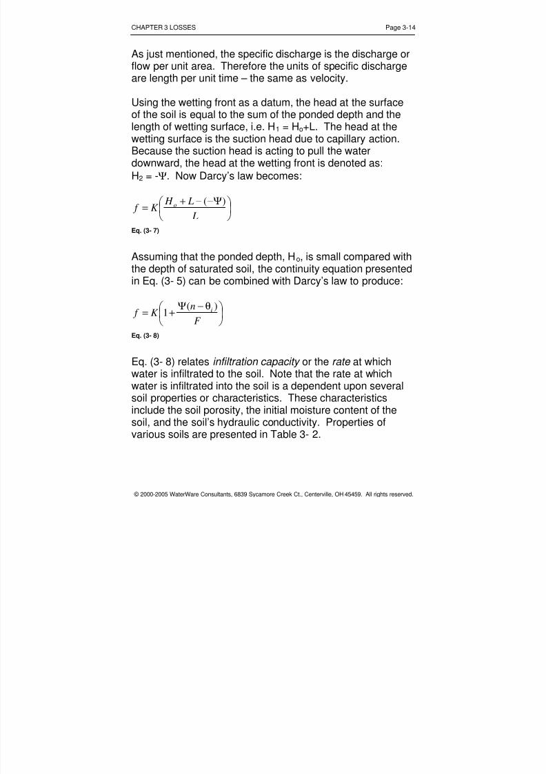
As just mentioned, the specific discharge is the discharge orflow per unit area. Therefore the units of specific dischargeare length per unit time – the same as velocity.

Using the wetting front as a datum, the head at the surfaceof the soil is equal to the sum of the ponded depth and thelength of wetting surface, i.e. H 1 = H o+L. The head at thewetting surface is the suction head due to capillary action.Because the suction head is acting to pull the waterdownward, the head at the wetting front is denoted as:H2 = -Ψ . Now Darcy’s law becomes:

Ψ−−+=

L L H K f o )(

Eq. (3- 7)

Assuming that the ponded depth, H o, is small compared withthe depth of saturated soil, the continuity equation presentedin Eq. (3- 5) can be combined with Darcy’s law to produce:

θ−Ψ

+=F

nK f i )(

1

Eq. (3- 8)

Eq. (3- 8) relates infiltration capacity or the rate at whichwater is infiltrated to the soil. Note that the rate at whichwater is infiltrated into the soil is a dependent upon several

soil properties or characteristics. These characteristicsinclude the soil porosity, the initial moisture content of thesoil, and the soil’s hydraulic conductivity. Properties ofvarious soils are presented in Table 3- 2.





Table 3- 2

Soil Type Porosity Saturated HydraulicConductivity (cm/hr)

SuctionHead (cm)

Sand 0.437 11.78 4.95

Loamy sand 0.437 2.99 6.13Sandy loam 0.453 1.09 11.01

Loam 0.463 0.34 8.89Silt loam 0.501 0.65 16.68

Sandy clay loam 0.398 0.15 21.85Clay loam 0.464 0.10 20.88

Silty clay loam 0.471 0.10 27.30Sandy clay 0.430 0.06 23.90Silty clay 0.479 0.05 29.22

Clay 0.475 0.03 31.63

Notice that Eq. (3- 8) provides an expression for theinfiltration capacity or rate. As will be shown in the nextsection, the infiltration depth is needed to determine theamount of excess precipitation. The infiltration depth can befound by noting that the infiltration rate is the time derivativeof the infiltration depth, i.e.:

θ−Ψ

+==F

nK

dt dF

f i )(1

Eq. (3- 9)

The infiltration depth can be found by integrating Eq. (3- 9)as shown below. Eq. (3- 9) has been simplified to facilitatethe mathematical computations.

( )( ) θ−Ψ+==

F

i

t

dF nF

F Kdt F

00

Eq. (3- 10)





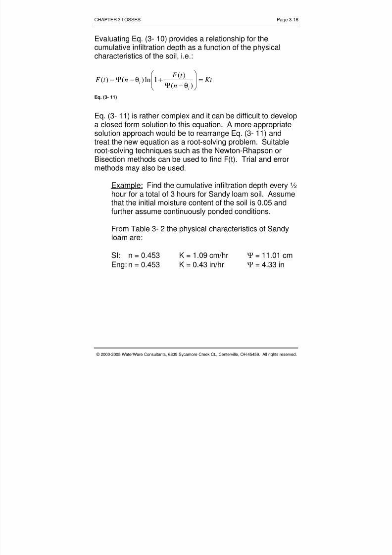
Evaluating Eq. (3- 10) provides a relationship for thecumulative infiltration depth as a function of the physicalcharacteristics of the soil, i.e.:

Kt n

t F nt F

ii

=

θ−Ψ+θ−Ψ−

)()(

1ln)()(

Eq. (3- 11)

Eq. (3- 11) is rather complex and it can be difficult to developa closed form solution to this equation. A more appropriatesolution approach would be to rearrange Eq. (3- 11) and

treat the new equation as a root-solving problem. Suitableroot-solving techniques such as the Newton-Rhapson orBisection methods can be used to find F(t). Trial and errormethods may also be used.

Example: Find the cumulative infiltration depth every ½hour for a total of 3 hours for Sandy loam soil. Assumethat the initial moisture content of the soil is 0.05 andfurther assume continuously ponded conditions.

From Table 3- 2 the physical characteristics of Sandyloam are:

SI: n = 0.453 K = 1.09 cm/hr Ψ = 11.01 cmEng: n = 0.453 K = 0.43 in/hr Ψ = 4.33 in





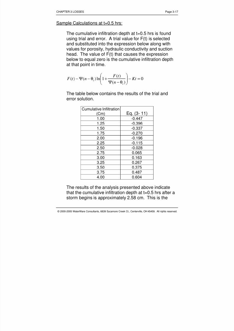
Sample Calculations at t=0.5 hrs:

The cumulative infiltration depth at t=0.5 hrs is foundusing trial and error. A trial value for F(t) is selectedand substituted into the expression below along withvalues for porosity, hydraulic conductivity and suctionhead. The value of F(t) that causes the expressionbelow to equal zero is the cumulative infiltration depthat that point in time.

0)(

)(1ln)()( =−

θ−Ψ

+θ−Ψ− Kt n

t F nt F

ii

The table below contains the results of the trial anderror solution.

Cumulative Infiltration(Cm) Eq. (3- 11) 1.00 -0.4471.25 -0.396

1.50 -0.3371.75 -0.2702.00 -0.1962.25 -0.1152.50 -0.0282.75 0.0653.00 0.1633.25 0.2673.50 0.375

3.75 0.4874.00 0.604

The results of the analysis presented above indicatethat the cumulative infiltration depth at t=0.5 hrs after astorm begins is approximately 2.58 cm. This is the





value that satisfies Eq. (3- 11). If the infiltration rate atany time is of interest, then Eq. (3- 8) can be used tofind this quantity. The solution procedure illustratedabove can be used to find the cumulative infiltrationdepth at other times.

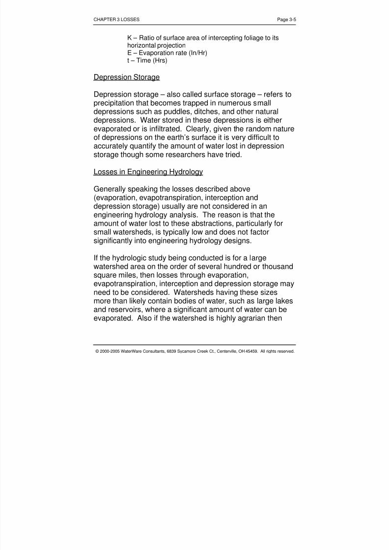
Continuously Ponded Conditions

The Green and Ampt formulation is based on theassumption that the soil is subjected to continuously pondedconditions. In other words, the availability of water always

exceeds the infiltration capacity. At the beginning of a stormthe infiltration capacity is at its highest while the rainfallintensity can be low at the start of a storm.

When the rainfall intensity is less than the infiltrationcapacity, all precipitation will be infiltrated and there will beno excess precipitation. When the rainfall intensity exceedsthe infiltration capacity then continuously ponded conditionsexist and there will be some runoff. If continuously pondedconditions are not present, then an adjustment must bemade in the cumulative infiltration values.

Phi Index

An alternate approach to specifying losses is to simplyassume that the loss is a constant value over the entireduration of the hydrologic simulation. This is called a Phi

Index or a simple abstraction. When the rainfall depth isequal to or exceeds the Phi Index, then the amount of rainfallequal to the index is assumed to be lost. Any excessprecipitation contributes to runoff. This approach is notrecommended unless good quality data on the losses withina watershed are available.





Time (Hrs)

I n c r e m e n t a l

E x c e s s

P r e c i p i t a t

i o n

( I n )

0 1 2 3 4 5 6 7 8

Phi Index

Figure 3- 4

Direct Runoff or Excess Precipitation

In order to develop a runoff hydrograph – which is a timehistory of watershed runoff – it is necessary to determine thedirect runoff. Recall that the direct runoff is also called theexcess precipitation. Throughout the remainder of thisreference manual these terms are used interchangeably.

Once all losses have been computed, then the direct runoffcan be found using a mass balance technique. The massbalance approach is illustrated in the expression below.

)()()( t Lt Pt R −=

Eq. (3- 12)

Where: R(t) – Cumulative excess precipitation at time t (In)P(t) – Cumulative precipitation that has fallen at time t (In)L(t) – Cumulative losses at time t (In)





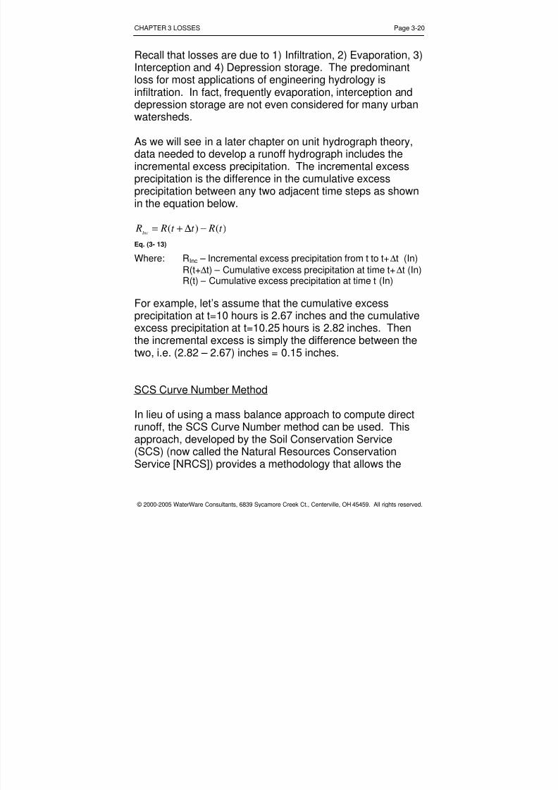
Recall that losses are due to 1) Infiltration, 2) Evaporation, 3)Interception and 4) Depression storage. The predominantloss for most applications of engineering hydrology isinfiltration. In fact, frequently evaporation, interception anddepression storage are not even considered for many urbanwatersheds.

As we will see in a later chapter on unit hydrograph theory,data needed to develop a runoff hydrograph includes theincremental excess precipitation. The incremental excessprecipitation is the difference in the cumulative excessprecipitation between any two adjacent time steps as shown

in the equation below.

)()( t Rt t R R Inc−∆+=

Eq. (3- 13)

Where: R Inc – Incremental excess precipitation from t to t+ ∆ t (In)R(t+ ∆ t) – Cumulative excess precipitation at time t+ ∆ t (In)R(t) – Cumulative excess precipitation at time t (In)

For example, let’s assume that the cumulative excessprecipitation at t=10 hours is 2.67 inches and the cumulativeexcess precipitation at t=10.25 hours is 2.82 inches. Thenthe incremental excess is simply the difference between thetwo, i.e. (2.82 – 2.67) inches = 0.15 inches.

SCS Curve Number Method

In lieu of using a mass balance approach to compute directrunoff, the SCS Curve Number method can be used. Thisapproach, developed by the Soil Conservation Service(SCS) (now called the Natural Resources ConservationService [NRCS]) provides a methodology that allows the





excess precipitation to be computed directly. The equationused to compute the excess precipitation is shown below.

( )( )St P

I t Pt R

a

8.0)()(

)(

2

+

−

=

Eq. (3- 14)

Where: R(t) – Cumulative excess precipitation at time t (In)P(t) – Cumulative precipitation that has fallen at time t (In)Ia – Initial abstraction (In)S – Maximum storage retention of the soil (In)

Eq. (3- 14) can be derived based on a few assumptions.

First though, let’s define some terms. The quantity P(t)represents the cumulative precipitation that has fallen up totime t. Note that the cumulative precipitation at time t isdirectly related to the temporal nature or distribution of thestorm. R(t) represents the cumulative amount of excessprecipitation or runoff at time t. The difference between P(t)and R(t) at time t is the amount of losses due to primarily toinfiltration that has occurred up to time t.

The maximum storage retention of the soil, S, represents themaximum amount of water that can be infiltrated into the soilafter runoff begins. The initial abstraction, I a , represents theamount of water that must be lost before any runoff canoccur. This water is lost to interception, depression storageand infiltration. One can think of this quantity as a tax thatmust be paid by the storm before any runoff can occur.

Let’s further define that the cumulative amount of water thatis infiltrated into the soil as F(t). Note that this quantity isdifferent than the initial abstraction, I a , since water continuesto be lost due to infiltration after the initial abstraction hasbeen satisfied.





As the precipitation approaches infinity, the following ratiosbecome equal to unity, i.e.

1lim =∞→ SF

P

Eq. (3- 15)

1lim =∞→ P

RP

Eq. (3- 16)

Eq. (3- 15) suggests that as the precipitation approachesinfinity, then the amount of water that is infiltratedapproaches the maximum soil storage capacity. In otherwords, no more water can be infiltrated, i.e. the soil iscompletely saturated and cannot hold any more water.Therefore the ratio of the infiltrated depth, F, and themaximum amount of water that can be infiltrated, S, equalsone.

Once the infiltration capacity of a soil has been “used-up”, allprecipitation will become direct runoff. Therefore, as shownby Eq. (3- 16), as the precipitation approaches infinity allrainfall will produce runoff so the ratio of runoff toprecipitation is equal to one.

As the precipitation depth approaches zero, the followingratios become zero.

0lim0

=→ S

F P

Eq. (3- 17)





0lim0

=→ P

RP

Eq. (3- 18)

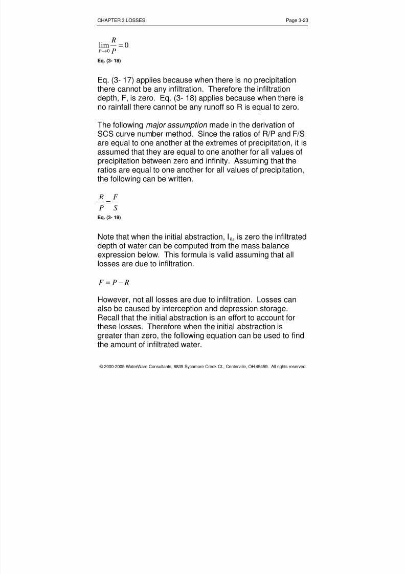
Eq. (3- 17) applies because when there is no precipitationthere cannot be any infiltration. Therefore the infiltrationdepth, F, is zero. Eq. (3- 18) applies because when there isno rainfall there cannot be any runoff so R is equal to zero.

The following major assumption made in the derivation ofSCS curve number method. Since the ratios of R/P and F/Sare equal to one another at the extremes of precipitation, it isassumed that they are equal to one another for all values ofprecipitation between zero and infinity. Assuming that theratios are equal to one another for all values of precipitation,the following can be written.

SF

P R

=

Eq. (3- 19)

Note that when the initial abstraction, I a , is zero the infiltrateddepth of water can be computed from the mass balanceexpression below. This formula is valid assuming that alllosses are due to infiltration.

RPF −=

However, not all losses are due to infiltration. Losses canalso be caused by interception and depression storage.Recall that the initial abstraction is an effort to account forthese losses. Therefore when the initial abstraction isgreater than zero, the following equation can be used to findthe amount of infiltrated water.





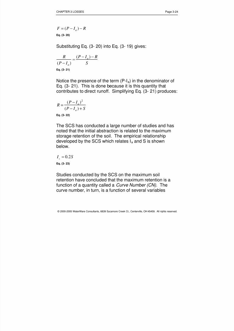
R I PF a−−= )(

Eq. (3- 20)

Substituting Eq. (3- 20) into Eq. (3- 19) gives:

S R I P

I P R a

a

−−=

−

)()(

Eq. (3- 21)

Notice the presence of the term (P-I a) in the denominator of

Eq. (3- 21). This is done because it is this quantity thatcontributes to direct runoff. Simplifying Eq. (3- 21) produces:

S I P I P

Ra

a

+−

−=

)()( 2

Eq. (3- 22)

The SCS has conducted a large number of studies and hasnoted that the initial abstraction is related to the maximumstorage retention of the soil. The empirical relationshipdeveloped by the SCS which relates I a and S is shownbelow.

S I a 2.0=

Eq. (3- 23)

Studies conducted by the SCS on the maximum soilretention have concluded that the maximum retention is afunction of a quantity called a Curve Number (CN) . Thecurve number, in turn, is a function of several variables





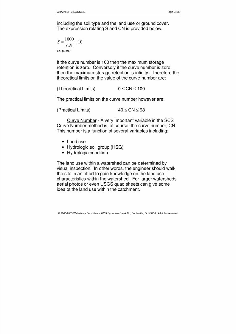
including the soil type and the land use or ground cover.The expression relating S and CN is provided below.

101000

−= CN S

Eq. (3- 24)

If the curve number is 100 then the maximum storageretention is zero. Conversely if the curve number is zerothen the maximum storage retention is infinity. Therefore thetheoretical limits on the value of the curve number are:

(Theoretical Limits) 0 ≤ CN ≤ 100

The practical limits on the curve number however are:

(Practical Limits) 40 ≤ CN ≤ 98

Curve Number - A very important variable in the SCSCurve Number method is, of course, the curve number, CN.This number is a function of several variables including:

• Land use• Hydrologic soil group (HSG)• Hydrologic condition

The land use within a watershed can be determined byvisual inspection. In other words, the engineer should walk

the site in an effort to gain knowledge on the land usecharacteristics within the watershed. For larger watershedsaerial photos or even USGS quad sheets can give someidea of the land use within the catchment.





The hydrologic soil group is a function of the soil type.Hydrologic soil groups can range from Group A which is awell-drained (low CN) soil to Group D which is a poorly-drained (high CN) soil. Hydrologic soil groups B and C fallbetween the two with HSG B having better drainagecharacteristics than HSG C.

County soil maps have been produced by the SoilConservation Service and can be used to find the names ofsoils that are in a specific watershed. With the names of thesoils known, one can access Appendix A in TechnicalRelease No. 55 (TR55) for the appropriate HSG.

Hydrologic condition refers to the effects of cover type andtreatment. Hydrologic conditions can be poor, fair or good.A soil that has a good hydrologic condition is one that haslow runoff potential for a given HSG and land use. Forexample, a meadow might have a hearty stand of grass thatwould reduce the runoff potential. Thus the grass wouldcreate a good hydrologic condition. The same meadow

could have places of rock outcropping which would increasethe runoff potential. This could cause a poor hydrologiccondition.

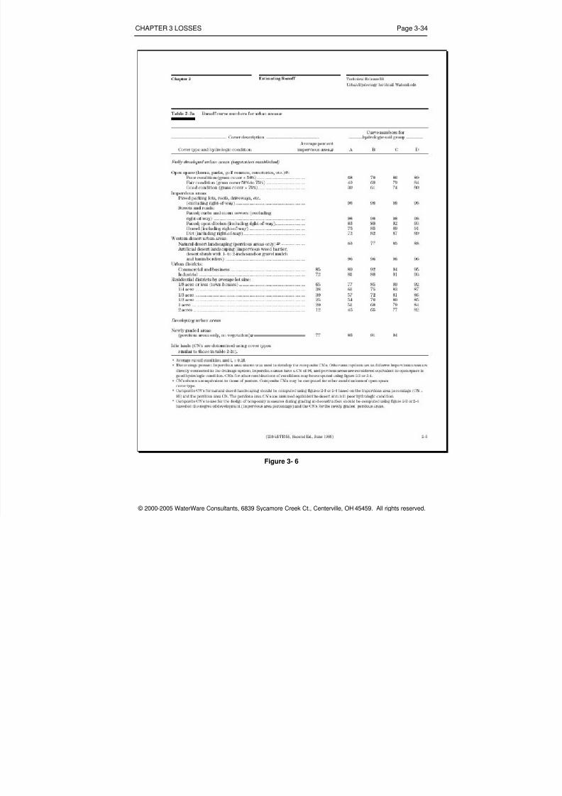
There are a number of available tables that can be used tofind the curve number for a given land use, HSG andhydrologic condition. Perhaps the most commonly usedtables are those found in Technical Release No. 55, i.e. theTR55 document. Table 2.2 in the TR55 publication providescurve numbers for a wide range of land use. Figure 3- 6shows a portion of this table. The TR55 document can bedownloaded from the Natural Resources ConservationService web site at:

http://www.wcc.nrcs.usda.gov/





Most published tables of curve number provide values thatrepresent average soil moisture. The term that describesthe relative amount of moisture in a soil is called theAntecedent Moisture Content (AMC). In engineeringhydrology there are three levels of AMC:

1. AMC I – dry soil2. AMC II – average moisture3. AMC III – wet soil

In some cases it may be necessary to adjust curve numberstaken from the literature to reflect the actual soil moisture.

The values presented in Table 3- 3 can be used for thispurpose.Table 3- 3

CN for AMC II CN for AMC I CN for AMC III100 100 10095 87 9990 78 9885 70 9780 63 9475 57 9170 51 8765 45 8360 40 7955 35 7550 31 7045 27 6540 23 6035 19 5530 15 5025 12 4520 9 3915 7 3310 4 265 2 170 0 0





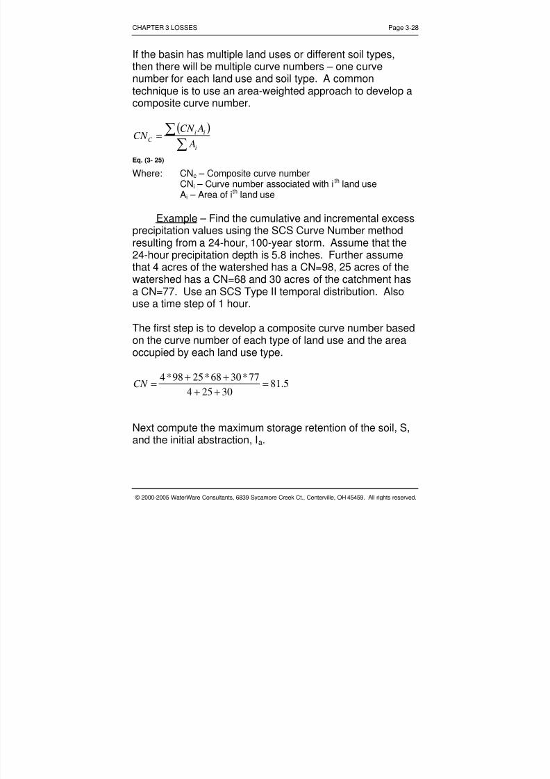
If the basin has multiple land uses or different soil types,then there will be multiple curve numbers – one curvenumber for each land use and soil type. A commontechnique is to use an area-weighted approach to develop acomposite curve number.

( )=

i

iiC A

ACN CN

Eq. (3- 25) Where: CN c – Composite curve number

CN i – Curve number associated with i th land useAi – Area of i th land use

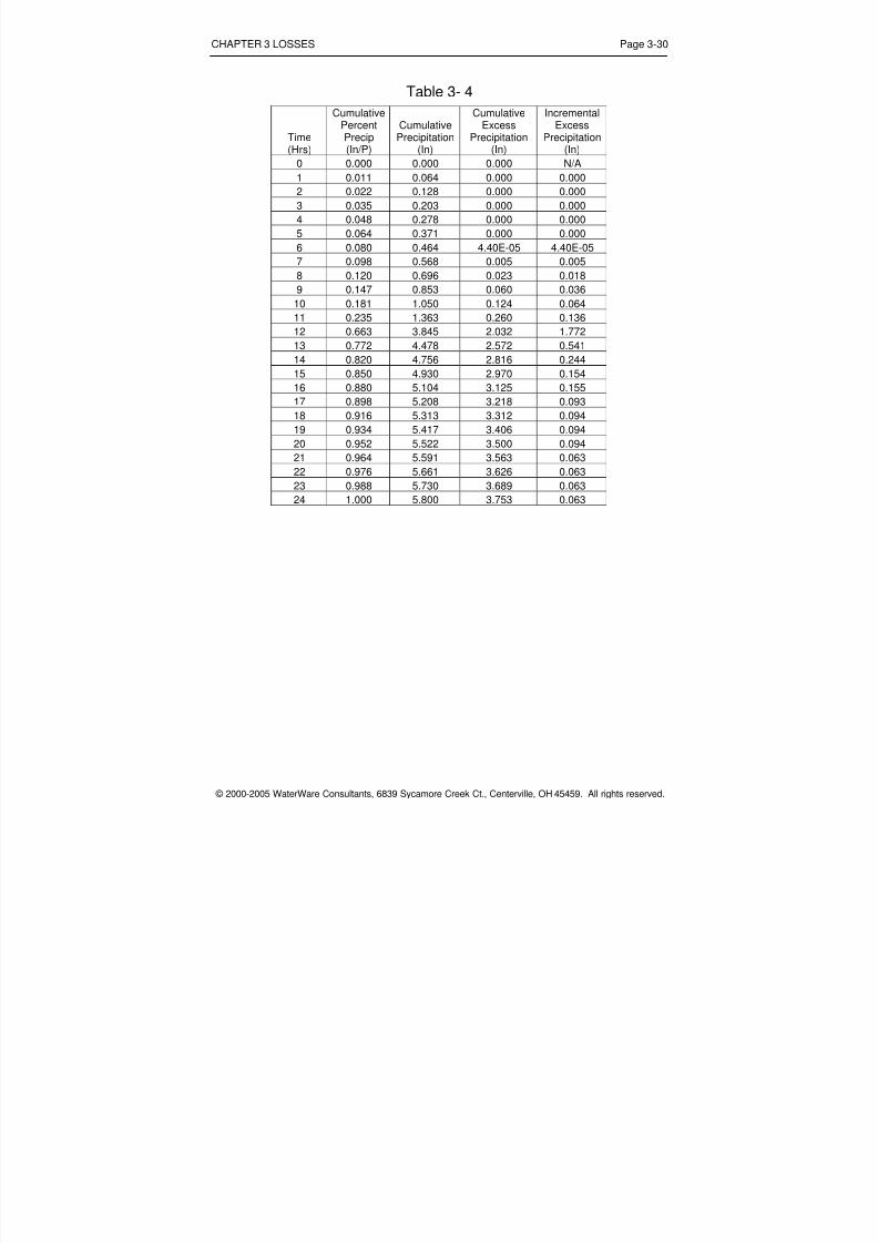
Example – Find the cumulative and incremental excessprecipitation values using the SCS Curve Number methodresulting from a 24-hour, 100-year storm. Assume that the24-hour precipitation depth is 5.8 inches. Further assumethat 4 acres of the watershed has a CN=98, 25 acres of thewatershed has a CN=68 and 30 acres of the catchment hasa CN=77. Use an SCS Type II temporal distribution. Alsouse a time step of 1 hour.

The first step is to develop a composite curve number basedon the curve number of each type of land use and the areaoccupied by each land use type.

5.8130254

77*3068*2598*4=

++

++=CN

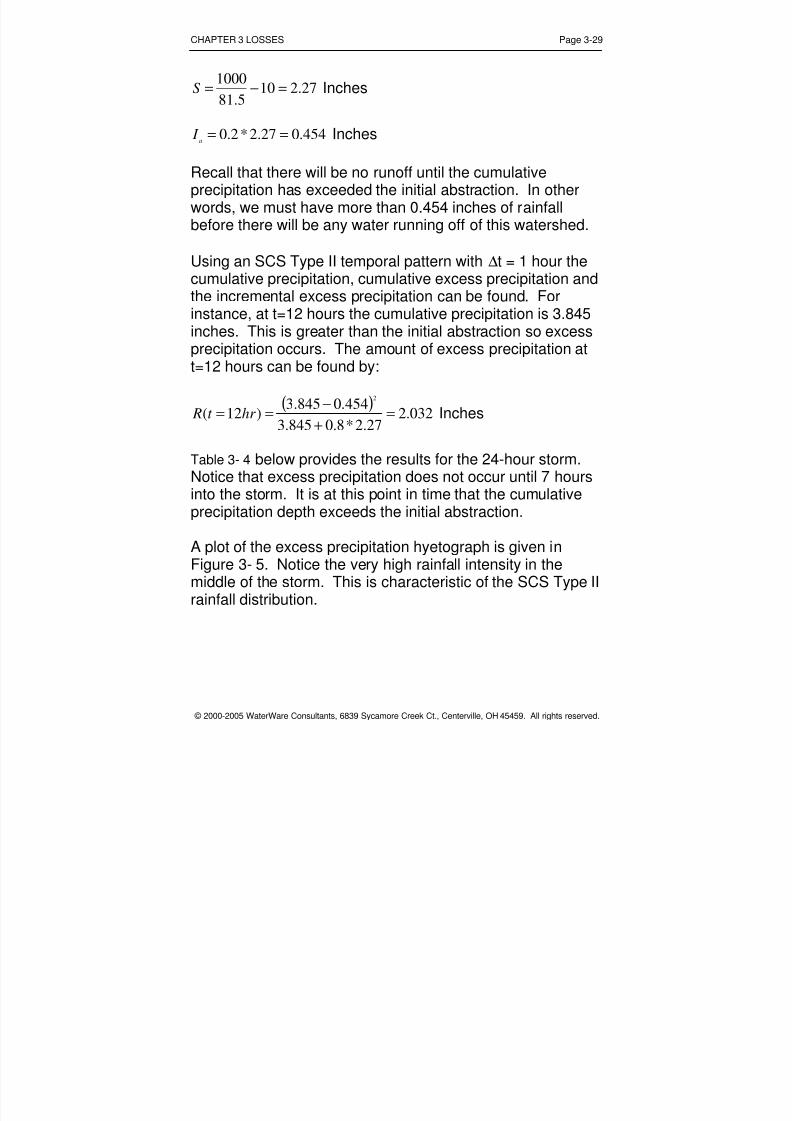
Next compute the maximum storage retention of the soil, S,and the initial abstraction, I a .





Table 3- 4

Time(Hrs)

CumulativePercentPrecip(In/P)

CumulativePrecipitation

(In)

CumulativeExcess

Precipitation(In)

IncrementalExcess

Precipitation(In)

0 0.000 0.000 0.000 N/A1 0.011 0.064 0.000 0.0002 0.022 0.128 0.000 0.0003 0.035 0.203 0.000 0.0004 0.048 0.278 0.000 0.0005 0.064 0.371 0.000 0.0006 0.080 0.464 4.40E-05 4.40E-057 0.098 0.568 0.005 0.0058 0.120 0.696 0.023 0.0189 0.147 0.853 0.060 0.036

10 0.181 1.050 0.124 0.064

11 0.235 1.363 0.260 0.13612 0.663 3.845 2.032 1.77213 0.772 4.478 2.572 0.54114 0.820 4.756 2.816 0.24415 0.850 4.930 2.970 0.15416 0.880 5.104 3.125 0.15517 0.898 5.208 3.218 0.09318 0.916 5.313 3.312 0.09419 0.934 5.417 3.406 0.09420 0.952 5.522 3.500 0.09421 0.964 5.591 3.563 0.06322 0.976 5.661 3.626 0.063

23 0.988 5.730 3.689 0.06324 1.000 5.800 3.753 0.063



CHAPTER 3 LOSSES


Excess Precipitation Hyetograph

0.000

0.200

0.400

0.600

0.800

1.000

1.200

1.400

1.600

1.800

2.000

1 2 3 4 5 6 7 8 9 10 11 12 13 14 15 16 17 18 19 20

Time (Hrs)

E x c e s s

P r e c

i p ( I n )

Figure 3- 5

Excess Precipitation Hyetograph





! CAUTION !

In some cases caution should be used with the SCS CurveNumber method. Depending upon the nature of the pre andpost developed conditions, it is possible that the postdeveloped curve number could be less than thepredeveloped curve number. This implies that the runoffunder post developed conditions would be less than thepredeveloped runoff. As a result, it would seem that nodetention is necessary.

Let’s assume that we are developing land that was farmed in

the past, but is now a fallow field with mostly bare soil. Let’sfurther assume that the soil falls within HSG B. Using Table2.2b from the TR55 document we would select apredeveloped curve number of CN=86. Now let’s supposethat we wish to develop the land into a residentialneighborhood with lots averaging 1/3 acre.

Note that the soil type has not changed. Therefore from

Table 2.2a from the TR55 document we would select a curvenumber of CN=72. This assumes, of course, that theaverage percent of impervious area within the watershed is30%. The post developed curve number is less than thepredeveloped curve number indicating that no detention isnecessary.

What we have not considered is the affect of constructionactivities on the surface crust. Again while the soil type doesnot change, construction equipment can compact the uppersoil crust thereby influencing the infiltration characteristics ofthe soil. Furthermore construction debris (depending uponits magnitude) could also affect the ability of the upper layerof soil to pass water.





For most reviewing agencies a condition such as this shouldraise a red flag. A competent engineer should examine therunoff characteristics of the watershed assuming ahydrologic soil group having poorer infiltrationcharacteristics. For example if the original soil is HSG B,then an analysis should be conducted assuming HSG C oreven HSG D. Detention basin designs can then bedeveloped based on any increase in the runoff.

While it may seem that the curve numbers for agriculturalareas are quite high, engineers must recognize that farmfields may be drained by tiles. It is not uncommon for

underground pipes to be installed in a farm field to facilitatedrainage of the field. For a field drained by tiles, theinfiltrated water can be quickly directed to a receivingstream. This behavior can be addressed by using a highercurve number. The engineer should try to determine if anarea once used for agriculture and now slated fordevelopment has underground tiles. Will these pipes beremoved during the construction process? What affect will

this have on the overall drainage characteristics of thewatershed?

In the final analysis, it is the experience and judgment of theengineer coupled with the knowledge the engineer has of thesite under question that helps to insure safe and adequatedrainage control. Moreover it is the obligation of thereviewing agency to insure that any drainage controlsproposed by the engineer are acceptable within the aimsand goals of the agency.




Figure 3- 6

chpt 3-abstractions or losses

Documents