Choosing smoothness parameters for smoothing

splines by minimizing an estimate of risk

Rafael A. Irizarry

Department of Biostatistics, Johns Hopkins University

615 N. Wolfe Street, Baltimore, Maryland 21205

rafa@jhu.edu, 410-614-5157, 410-955-0958 (fax)

SUMMARY. Smoothing splines are a popular approach for non-parametric regression problems. We

use periodic smoothing splines to fit a periodic signal plus noise model to data for which we as-

sume there are underlying circadian patterns. In the smoothing spline methodology, choosing an

appropriate smoothness parameter is an important step in practice. In this paper, we draw a con-

nection between smoothing splines and REACT estimators that provides motivation for the creation

of criteria for choosing the smoothness parameter. The new criteria are compared to three existing

methods, namely cross-validation, generalized cross-validation, and generalization of maximum

likelihood criteria, by a Monte Carlo simulation and by an application to the study of circadian pat-

terns. For most of the situations presented in the simulations, including the practical example, the

new criteria out-perform the three existing criteria.

KEY WORDS: Non-parametric smoothing, REACT estimators, Smoothing splines, Smoothness pa-

rameter.

1

1 Introduction

Most organisms generate physiological and behavioral measurements with oscillations (Re-

finetti and Menaker 1992). It is quite common for these oscillations to have a 24 hours

period. In this case, we refer to them as circadian patterns or circadian rhythms. Various

researchers have used statistical models to describe data believed to contain circadian pat-

terns, see for example Greenhouse, Kass,and Tsay (1987) and Wang and Brown (1996).

Modeling circadian patterns can have practical applications, for example Irizarry et al.

(2001) used circadian pattern estimates to assess homeostasis in mice. In general, one is

interested in describing circadian patterns as smooth functions of times but the data used to

estimate these patterns usually contains noise. The problem of estimating circadian shapes

is commonly viewed as a non-parametric regression problem.

Smoothing splines are a popular approach for non-parametric regression problems. For

example, the widely used S-Plus function gam() uses local regression lo() and smooth-

ing splines s() as built-in smoothers (Hastie 1993). Many authors, Schoenberg (1964),

Reinsch (1967), Wahba and Wold (1975), and Silverman (1985) to name a few, have stud-

ied smoothing splines and demonstrated desirable theoretical properties. Some, for exam-

ple Rice and Rosenblatt (1983), have developed asymptotic results for smoothing splines.

For a good review of spline methods in statistics see Eubank (1988) and for a complete

theoretical treaty see Wahba (1990).

When using smoothing splines one does not need to choose the location of knots and

2

the smoothness of the estimate is controlled via one parameter, usually referred to as the

smoothness parameter and denoted in this paper with λ. This makes the procedure easy to

implement in practice. In Section 2 we describe smoothing splines in more detail.

Choosing an appropriate λ is an important step in practice. A λ that is “too close to

zero” will yield an estimate practically equivalent to the data, and a λ that is “too big”

will produce an estimate practically equivalent to the linear regression estimate of the data.

Cross validation (CV) and generalized cross-validation (GCV) (Craven and Wahba (1979))

are popular approaches for finding an appropriate criterion and are the two procedures

available through the S-Plus function smooth.spline(). These procedures have been

criticized for choosing λs that are “too small” (Hastie and Tibshirani, page 52) and other

approaches have been proposed, for example Wahba’s (1985) Generalized Maximum Like-

lihood (GLM) criterion. In Section 3, for a regular time series periodic signal plus noise

model, we establish a connection between smoothing splines and Beran’s (2000) Risk Es-

timation After Coordinate Transform (REACT) estimators and use it to motivate a new cri-

terion for choosing the smoothness parameter. As described in Section 4 this new method,

which we will refer to as the REACT criterion for choosing the smoothness parameter, is

convenient from a computational perspective. Furthermore, we compare its performance

by comparing mean squared error (MSE), through a Monte Carlo simulation, to CV, GCV,

and GLM. In Section 5 we compare the methods through a real-data example.

3

2 Smoothing splines

Consider the signal plus noise model

yi = s(ti) + εi, i = 1, . . . , n, t1 < . . . < tn ∈ [0, 1] (1)

where ε = (ε1, . . . , εn)′ ∼ N(0, σ2In×n), σ2 is unknown and s some function in the

so-called Sobolev Hilbert space of functions W m2 [0, 1] with domain [0, 1], the derivatives

s(l), l = 1, . . . ,m− 1 absolutely continuous, and bounded s(m). In practice, s(t) can repre-

sent the underlying circadian pattern and ε represents measurement error and environmental

variation.

We will denote y = (y1, . . . , yn)′ and, to follow Beran’s (2000) notation, η = s(t1), . . . , s(tn)′.

The smoothing spline estimate is defined as the function sλ ∈ Wm2 [0, 1] yielding the ηλ that

minimizes a penalized least squares criterion,

1

n|y − η|2 + λ

∫ 1

0

s(m)(u)2 du (2)

with |y−η|2 =∑n

i=1 yi − s(ti)2 . Throughout the text we will be using the hat notation,

for example ξ, to denote estimates in general. In different parts of the text the meaning of,

say, ξ changes. However, the meaning should be clear from the context.

For m = 2, Reich (1967) proved that, given a λ, the solution to minimizing (2) is

a natural cubic spline with knots at t1, . . . , tn. This implies that we can write the η that

minimizes (2) as ηλ = N(N′N+λΩ)−1Ny where N and Ω are n×n matrices defined by

the basis functions for the space of natural cubic splines with knots at t1, . . . , tn (see Buja,

4

Hastie, and Tibshirani 1989). Using basic matrix algebra tricks we can find n× n matrices

U and Λ, with Λ diagonal, such that we can re-write η as

ηλ = U(In×n − λΛ)−1U′y (3)

Notice (In×n−λΛ)−1 is a diagonal matrix and later we denote the vector of diagonal entries

as f(λ).

Becuase of the nature of the data described in Section 5 and because circadian patterns

are periodic we consider the case of periodic smoothing splines for regular time series with

equally spaced knots. Furthermore, describing the REACT methodology for choosing the

smoothness parameter can be done in a simple fashion for this case. However, in Section 6

we describe how this method can be extended to the general case is a straight-forward way.

2.1 Periodic smoothing splines

In this section we consider the case where s ∈ W m2 [0, 1] is periodic, i.e. s(0) = s(1) and

s(l)(0) = s(l)(1), l = 1, . . . ,m, and the data is a regular time series, i.e. ti = i/n, i =

1, . . . , n. As noted by Wahba (1990), for a given λ, the periodic function in W m2 [0, 1] that

minimizes (2) is well approximated by a function of the form

sλ(t) = a0 +

n/2−1∑

j=1

aj

√2 cos(2πjt) +

n/2−1∑

j=1

bj

√2 sin(2πjt) + an/2 cos(πnt). (4)

Let UDFT be the n× n orthogonal discrete Fourier transform (DFT) matrix defined by

Ui,1 = n−1/2, i = 1, . . . , n

5

Ui,2j = (2/n)1/2 cos(2π j ti), i = 1, . . . , n, j = 1, . . . , n/2− 2

Ui,2j+1 = (2/n)1/2 sin(2π j ti), i = 1, . . . , n, j = 1, . . . , n/2− 1

Ui,n = n−1/2 cos(πi), i = 1, . . . , n (5)

and denote z = U′DFTy and ξ = U′

DFT η. Notice that z is the spectral decomposition of

y. We can use Fourier’s theorem to show that for functions of the form (4), minimizing (2)

is equivalent to minimizing

1

n|z− ξ|2 +

λ

n

n/2−1∑

j=1

(a2j + b2

j)(2πj)2m +1

2a2

n/2(πn)2m

(6)

with |z−ξ|2 =∑n/2

j=0(aj−aj)2+∑n/2−1

j=1 (bj−bj)2, where (a0, a1, b1, . . . , an/2−1, bn/2−1, an/2) ≡

z, and easily show that the value ξ that minimizes (6) is f(λ)z, with f(λ) a n−dimensional

vector and the multiplication component-wise (as in S-Plus or matlab). Furthermore, taking

the derivative of (6) and solving for 0 gives us, what we will call, the shrinkage coefficients

f(λ) = f0, f1(λ), f1(λ), . . ., fn/2−1(λ), fn/2−1(λ), fn/2(λ)′ in closed-form, with

f0 = 1, fj(λ) = 1+λ(2πj)2m−1, j = 1, . . . ,n

2−1, fn/2(λ) = 1+0.5λ(πn)2m−1. (7)

Because UDFT is an orthonormal transformation we have that the estimator that minimizes

(2) is UDFT f(λ)z.

Notice that we are assuming that n is even. This is done without loss of generality. If n

were odd, all the above remains the same except n/2− 1 becomes (n− 1)/2 and the terms

indexed by n/2 are ignored.

In summary, we have noticed that for a regular time series periodic signal plus noise

6

model, the smoothing spline estimate of s, for a given λ, can be well approximated by

UDFT diag[f(λ)]U′DFTy and we have closed form expressions for UDFT and f(λ). This

can be viewed as “filtering” the data y using a filter defined by the f which are in turn

defined by λ and the smoothing spline procedure.

As mentioned, choosing λ is an important step in practice. A popular way of precisely

defining an optimal λ is to use the expected MSE or risk, that is to choose the λ yielding

the estimate ηλ that minimizes

R(ηλ,η, σ2) =1

nE|ηλ − η|2. (8)

The CV and GCV criteria try to estimate the λ that provides the smoothing spline estimate

ηλ that minimizes (8). In the following sections we describe the REACT criterion for

choosing λ.

3 REACT

For data y arising from a model like (1), Beran (2000) studies the linear shrinkage estimates

of ξ = U′η defined by ξ(f) ≡ fz, f ∈ [0, 1]n with ξ(f) component-wise as in the

previous section and U is an orthonormal basis transformation. This implies that the risks

R(η,η, σ2) = R(ξ, ξ, σ2) are identical, so a good estimate of ξ will provide an estimate

for η that is just as good. In Beran’s approach, the transformation U is chosen to be

an economical basis. By economical basis we mean that we expect only the first few

components of ξ to be much different from 0 in absolute value. If this is the case, we

7

can reduce the risk by shrinking the higher components of z (the zis for which we expect

ξi to be close to 0) towards 0. Notice that for a specific component, the amount of bias

we add, (1 − fi)2ξ2

i is small if ξi is close to 0, and the variance is reduced by a factor

of f 2i , which is substantial if the amount of shrinkage is significant, i.e. fi is close to 0.

Once an appropriate economical basis has been chosen, REACT is data-driven procedure

that chooses a vector of shrinking coefficients f that minimize an estimate of risk, and

defines the REACT estimator of ξ as ξ(f) = f z. This implies η(f) = Uξ(f) is the

REACT estimate for η. Beran (2000) describes ways to choose f so that ξ(f) has desirable

asymptotic properties.

Turning our attention back to periodic smoothing splines, from (5) notice that UDFT has

columns that are of increasingly higher frequency, i.e. columns of decreasing smoothness.

If in fact s is smooth, then only the first few components of ξ = U′DFT η will be “much

different” from zero in absolute value. For a given λ we notice that the smoothing spline

estimate can be thought of as a REACT estimator UDFT ξ(λ) with z = U′DFTy and ξ(λ) =

f(λ)z with the multiplication component-wise. Expression (7) shows that this estimate

automatically shrinks the “high-frequency” components of η. The bigger λ the more we

shrink. Now we will see how the ideas used to choose f in REACT estimation can be used

to select appropriate λs for smoothing splines.

For any m × 1 vector x, let sum(x) =∑m

i=1 xi and ave(x) = m−1sum(x) and notice

8

we can write the risk of ξ(f) = fz as

R(ξ(f), ξ, σ2) = ave[σ2f2 + ξ21− f2] (9)

with the multiplication component-wise as before. Ideally, if we knew the risk function (9),

we would estimate ξ with f z with f the f ∈ [0, 1]n minimizing (9). However, this ideal

linear estimator ξ is unrealizable in practice because ξ and σ2 are unknown. Beran (2000)

considers

R(ξ(f), z, σ2) = ave[f − g2z2] + ave[σ2g], (10)

with g = 1 − σ2/z2 and σ2 a “trust-worthy” estimator of σ2, as a surrogate for the risk

defined in (9) in identifying the best candidate estimators. Beran (2000) points out that

the value f = g that minimizes (10) is inadmissible but that by restricting the space of fs

over which we minimize (10) we obtain estimates with desirable properties (see Beran and

Dumbgen (1998) and Beran (2000) for details). If we restrict the space of fs to vectors

with the form defined by (7) and determined by λ then our REACT estimator is equivalent

to a smoothing spline estimate. Furthermore, these estimates have desirable asymptotic

properties as described in the Appendix. This motivates, what we call, the REACT criterion

for choosing smoothing parameters that works by constraining the f with (7), denoting it

f(λ), and choosing λ by

λ = arg minλ∈[0,∞]

ave[f(λ)− g2z2], (11)

with g and σ2 defined as in (10). This in turn defines the estimates ξ(λ) = f(λ)z and

9

η(λ) = UDFT ξ(λ). Notice that for periodic smoothing splines we have

ave[f(λ)− g2z2] ∝n/2−1∑

j=1

(

1− σ2

aj

)

− fj(λ)

2

a2j +

n/2−1∑

j=1

(

1− σ2

bj

)

− fj(λ)

2

b2j

+

(

1− σ2

an/2

)

− fn/2(λ)

2

a2n/2. (12)

and finding λ can be thought of as an example of estimating a parameter λ using weighted

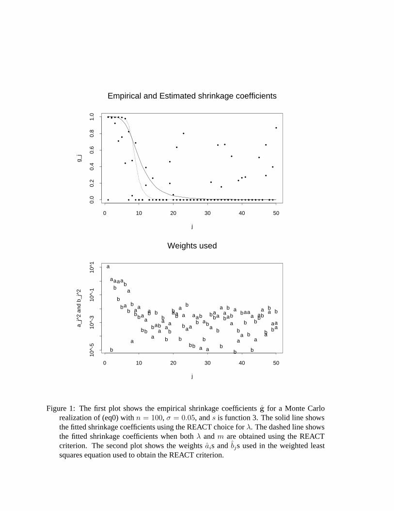
least squares where our data are the empirical shrinkage estimates g. In Figure 1 we see

plots showing an example of the function 1 + λ(2πj)2m−1 fitted to g and the weights

used in the weighted least squares equation.

Obtaining λ is computationally simple. In S-Plus the ajs and bjs are obtained using the

function fft() and minimizing (12) can be done with ms() or nlminb(). The final

estimate η can be obtained with fft(...,inv=T).

3.1 Estimating σ2

Notice that without an estimate η and with only one observation for each s(ti), i = 1, . . . , n

we don’t have a way to construct an estimate of σ2 based on residuals. The first difference

variance estimator (Rice (1984))

σ2 = 2(n− 1)−1

n∑

i=2

(yi − yi−1)2

provides an estimate that is not based on residuals. In practice, the procedure presented

in the previous section depends heavily on this estimate. In certain circumstances, such

as cases where σ2 is small compared to∫ 1

0s(t)2 dt, σ2 may provide an estimate that is

10

“too big”. In this Section we propose an iterative procedure that permits us to “update” the

estimate of σ2.

Start with the first difference estimate σ2(0) and use it in the REACT criterion to obtain

λ(0). Now we have a fitted model and can obtain residuals which we can use to form an

updated estimate of σ2. We assume E(η − η) ≈ 0 and approximate

E|y − η|2 = E[y′Uf(λ)U′′Uf(λ)U′y] ≈ (n− dfλ)σ2.

We refer to dfλ = sumf(λ)2 as the effective degrees of freedom. We then construct a new

estimate of σ2 with

σ2(1) = (n− dfλ)

−1|y − η(0)|2.

Continue this iterative procedure until |η(k)− η(k−1)| < δ with δ some small threshold.

We will refer to the λ obtained with this method as the REDACT choice, where the D

stands for “dynamic”. When no iterations are performed REDACT reduces to REACT.

3.2 Choosing m

The value of m is usually set at 2, mainly because it is the highest value of m for which the

space of smoothing spline solutions is of dimension n when knots are assigned to the design

points t1, . . . , tn. This makes the choice of m = 2 practical. However, once the problem

of choosing a λ has been reduced to (11), the shrinkage coefficients not only depend on

λ but on m and we could minimize (12) over (λ,m) ∈ [0,∞] × 1, 2, . . .. In fact if we

are willing to interpret fractional derivatives (McBride 1986) we can minimize (12) over

11

(λ,m) ∈ [0,∞]× [1,∞). As we will see in the following section, simulations suggest that

this procedure performs well. In this paper we will refer to these criteria as REACTm and

REDACTm.

4 Simulations

We have defined a new way of choosing the smoothness parameter for smoothing splines.

In this section we compare the REACT, REDACT, REACTm, and REDACTm criteria for

choosing λ to CV, GCV, and GML using a Monte Carlo simulation. We consider 4 func-

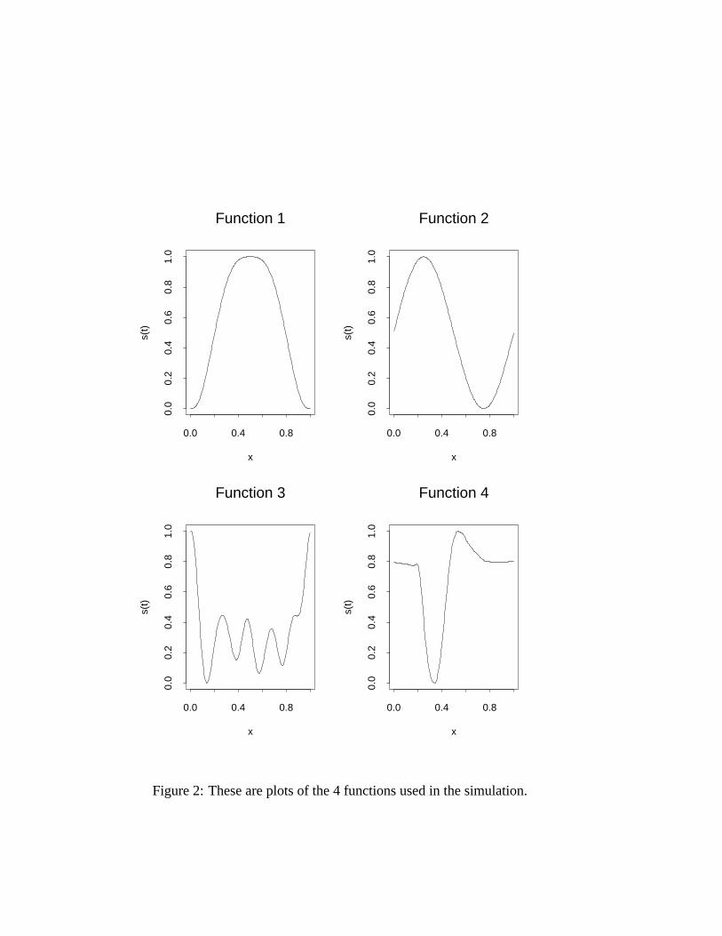
tions with 4 different degrees of “smoothness”. The first three functions are: s1(t) =

(1 − |2t − 1|3)3, s2(t) = sin(2πt), and s3(t) =∑8

j=1 ρk cos(2πt + φk) where the ρks and

φks are chosen from a uniform distribution on (0,1). The fourth function is an interpolation

of a local regression fit to the motorcycle data presented in Silverman (1985). In Figure 2

these functions are shown. Notice that all functions have been rescaled to have range [0,1].

For each function we create 100 simulations based on model (1) with n = 50, 100

and 250 and with σ = 0.025, 0.05, 0.1, 0.5 and 1. For each simulation we fit a periodic

smoothing spline with m = 2 and choose the smoothing parameter with REACT, REDACT,

CV (which in this case is equivalent to GCV), and GML. We also fit a periodic smoothing

spline and choose both λ and m with REACTm and REDACTm. We compare the average

MSE over the 100 simulations and also look at how frequently each procedure chooses

a λ producing an estimate with lower MSE than GCV, which is the default of the S-Plus

12

function smooth.spline(). The results of the simulation are presented in Tables 1, 2,

3, and 4 for functions 1, 2, 3, and 4 respectively. The GML works best when the noise has

large variance, i.e. σ = 0.5. However, in general the best performing criteria are REACTm

and REDACTm. For function 4, the roughest function, REACT and REDACT perform

better than REACTm and REDACTm except for small values of n and σ in which the

GCV performs slightly better. The REACT criterion is not always improved by the iterative

choice of σ2. As we would expect, the iterative versions seem to make an improvement

when the variance is small.

Notice that for the comparison with n = 50, σ = 0.05 for function 1 we have that the

CV criterion has a smaller average MSE than the REACT criterion but that the REACT

criterion chooses better λ for a larger percent of the simulations. This of course has to do

with the randomness of the simulation, but also with the fact that it is quite common for a

particular criterion to have a few very bad performances that bring the MSE up, but apart

from these it performs well.

Finding the λ minimizing the GML was not computationally possible in all cases. A

zero in the λ columns in the tables means no convergence was achieved. For function 3

and 4 convergence for the GML was so rare we removed it from the comparison. The code

generating these simulations are available in the Software section of the author’s web page:

http://www.biostat.jhsph.edu/∼ririzarr

13

5 An Example

We have activity measurements taken every 30 minutes from an AKR mouse. AKR mice

are one of many animals whose activity patterns are circadian. Furthermore, our scientific

intuition tells us that this pattern is probably a smooth, up-during-the-night down-during-

the-day pattern (these mice are nocturnal), it thus makes sense to model the data obtained

from these animals with a model like (1).

Physiologist have found that the shape of this circadian pattern can be used, for ex-

ample, to assess an animals health. Therefore, finding estimates of the smooth circadian

pattern is useful in practice. In Irizarry et al. (2001) the shape of the circadian pattern is

used to assess homeostasis.

We observe this mouse for 47 different days, thus we can consider each of these time

series as an independent identically distributed outcome of model (1). Averaging over the

47 days provides an unbiased estimate of η for which it is easy to obtain point-wise standard

errors. Considering this average to be the evaluations of the “true” s(t) at t1, . . . , tn permits

us to assess how well our smoothing splines estimate would have performed had we only

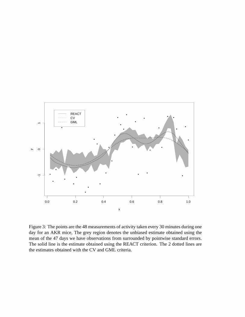
had one day of data. In Figure 3 we compare the estimates obtained with the λ chosen

by CV and GML with REACT. Notice REACT chooses a smaller λ that results in a less

smooth fit that appears to be more appropriate. Noitce in particular that only with the

REACT estimator do we see “two bumps”. We know the second bump is “real” because

we have observed the animals being active preparing there nest before sleeping.

14

If we obtain fits for each of the 47 days and obtain the MSE of each fit using the average

of 47 day estimate as the true s(t) we find that REACT has smaller MSE 29 times (62%)

and has a smaller average MSE.

6 Extensions

In Section 3 we motivated and defined the REACT criterion for periodic smoothing splines

with equally spaced knots. Extending to the general case is relatively straight-forward.

Notice that in Section 2.1 we use a transformation matrix UDFT for which we can form

linear shrinkage coefficients in the context of Beran (2000) in closed form. In the general

case the vector f(λ) would be the diagonal entries of (In×n − λΛ)−1. From here we can

proceed to define f(λ) as in (7) but now with fj(λ) = 1 + λΛj−1, j = 1, . . . , n with

Λj the diagonal entries of Λ and then proceed as before. The procedure is no longer as

convenient from a computational stand-point because we have to compute the Λ and U

matrices of (3) but still quite practical given that S-Plus has functions such as qr() and

eigen(). However, notice that minimizing over m is not as straight-forward.

In Section 3.2 we suggested that we should use the REACTm criterion to choose λ and

m. By doing this we are essentially changing not only the penalty multiplier but the penalty

itself. This idea has recently been explored in great detail by Heckman and Ramsay (2000).

The authors find that by considering different penalty criteria, estimates that perform well

are obtained. The procedure described in this paper can be easily extended to be used with

15

the procedure defined by Heckman and Ramsey. Notice in particular that the choices of

m, shown in Tables 1–4, are between 3 and 8, which suggest that the smoothing spline

methodology can be improved by changing the penalty criteria. This is in close agreement

with the penalty criteria suggested by Heckman and Ramsay.

Appendix: Theoretical Support

One can use Theorems 2.1 and 2.2 in Beran and Dumbgen (1998) to prove that minimizing the

estimated risk (10) is asymptotically equivalent to minimizing the risk (9). The details of the results

presented here can be found in Beran (unpublished manuscript).

If we define F to be the class of shrinkage coefficients f(λ) satisfying (7) it is easy to see

that F is a closed subset of the monotone shrinkage class FMS defined by Beran (2000). Further-

more, because for each element of this subset there is exactly one λ that defines it, it is completely

characterized by λ ∈ [0,∞]. If we assume σ2 is consistent in that, for every r > 0 and σ2 > 0

limn→∞

supave(ξ

2

)≤σ2r

E|σ2 − σ2| = 0

then one can show that for any r > 0 and σ2 > 0

limn→∞

supave(ξ

2

)≤σ2r

E| minλ∈[0,∞]

R(ξ(λ), ξ, σ2)− R(ξ(λ), z, σ2)|

with λ the REACT choice. Notice as the number of observations n goes to infinity we are taking a

sup over all functions s producing n-dimensional vectors ξ = Uη, with η the observed values of

s as defined in Section 2, with constrained average variability. Thus this result is not related to the

prior-belief that s is smooth. A result that supports the use of the U defined by smoothing splines

16

together with the REACT choice of λ when one is dealing with smooth functions follows. For every

b ∈ (0, 1), σ2 > 0, and r > 0 consider the ball of smooth functions

B(r, b, σ2) = ξ : ave(ξ2)/σ2 ≤ r and ξi = 0 for i > bn.

In the case of periodic splines, this ball contains functions for which the (1 − b) × 100% highest

frequency components are not present. The smaller b the smoother the functions in B(r, b, σ2).

Given this assumption one can use Theorem 4 in Beran (2000) to find that the asymptotic mini-

max quadratic risk over all estimators of η is σ2rb/(r+b) and the estimators defined by the REACT

choice of λ reach this bound:

limn→∞

supξ∈B(r,b,σ2)

R(ξ(λ), ξ, σ2) = σ2rb/(r + b)

In practice, we don’t necessarily expect the smooth functions s to be in any of the balls defined

above. However, in the author’s experience, from looking at plots of z for different data-sets, it

seems to be a reasonable approximation. A result that somehow assumes ξi ≈ 0 for i > bn would

be closer to what we find in practice. However, this is left as future work.

References

Beran, R. (unpublished manuscript) Available at <http://www.stat.berkeley.edu/∼beran/pls.pdf>

Beran, R. (2000). REACT scatterplot smoothers: Superefficiency through basis economy. Journal

of the American Statistical Association 95, 155–171.

Beran, R. and DUMBGEN, L. (1998), Modulation of Estimators and Confidence Sets. The Annals

of Statistics, 26, 1826–1856.

17

Buja, A., HASTIE, T., and Tibshirani, R. (1989), Linear smoothers and additive models (with dis-

cussion). Annals of Statistics 26, 1826-1856.

Craven, P. and Wahba, G. (1979), Smoothing noisy data with spline functions. Numerische Mathe-

matik 31, 377–403.

Eubank, R.L. (1988), Smoothing Splines and Nonparametric Regression. New York: Marcel Decker.

Greenhouse, J. B., Kass, R. E., and Tsay, R. S. (1987). Fitting nonlinear models with ARMA errors

to biological rhythm data. Statistics in Medicine 6, 167–183.

Hastie, T. J. (1993). Generalized Additive Models. In Chambers, J. M. and Hastie, T. J., editors,

Statistical Models in S, chapter 7, pages 249–307. Chapman & Hall, New York.

Heckman, N.E. and Ramsay, J.O. (2000). Penalized regression with model-based penalties. The

Canadian Journal of Statistics 28, 241–258.

Irizarry, R.A. , Tankersley, C.G., Frank, R., and Flanders, S.E. (2001). Assessing Homeostasis

through Circadian Patterns. Biometrics 57, 1228–1238.

McBride, A. C. (1986), Fractional Calculus. New York: Halsted Press.

Refinetti, R. and Menaker, M. (1992). The circadian rhythm of body temperature. Physiology &

Behavior 51, 135–140.

Reinsch, C. (1967) Smoothing by spline functions. Numererisch Mathematik 10, 177–183.

Rice, J.A. (1984), Bandwidth choice for nonparametric regression. Annals of Statistics 12, 1215–

1230.

Rice, J.A. and Rosenblatt, M. (1983), Smoothing splines, regression, derivatives, and convolution.

Annals of Statistics 11, 141-156.

Schoenberg, I.J. (1964), Spline functions and the problem of graduation. Proceedings of the Na-

18

tional Academy of Science USA 52, 947–950.

Silverman, B.W. (1985) Some Aspects of the spline smoothing approach to non-parametric regres-

sion curve fitting. Journal of the Royal Statistical Society B 47, 1–52.

Wahba, G. (1985). A Comparison of GCV and GML for Choosing the Smoothness Parameter in

the Generalized Spline Smoothing Problem. The Annals of Statistics 13, 1378–1402.

Wahba, G. (1990), Spline Models for Observational Data, CBMS-NSF Regional Conference Series,

Philadelphia: SIAM.

Wahba, G. and Wold, S. (1975), A completely automatic French curve: fitting spline functions by

cross-validation. Communications in Statistics 4, 1–17.

Wang, Y. and Brown, M. B. (1996). A flexible model for human circadian rhythms. Biometrics 52,

588–596.

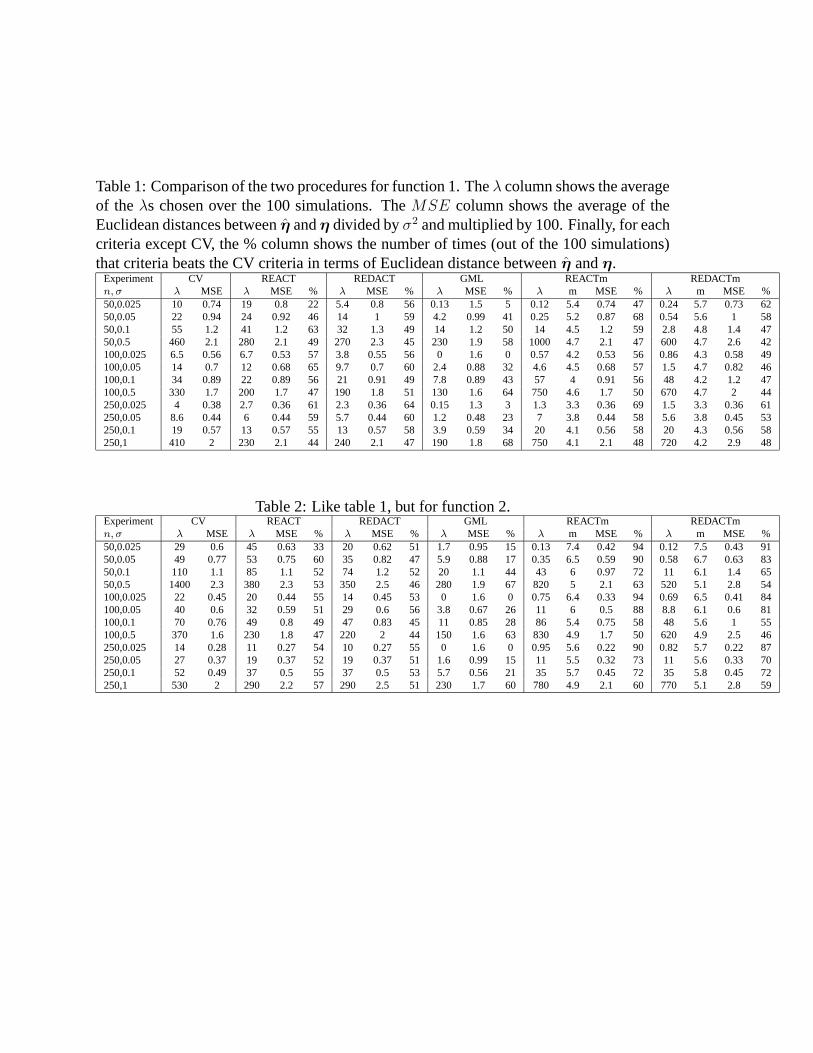
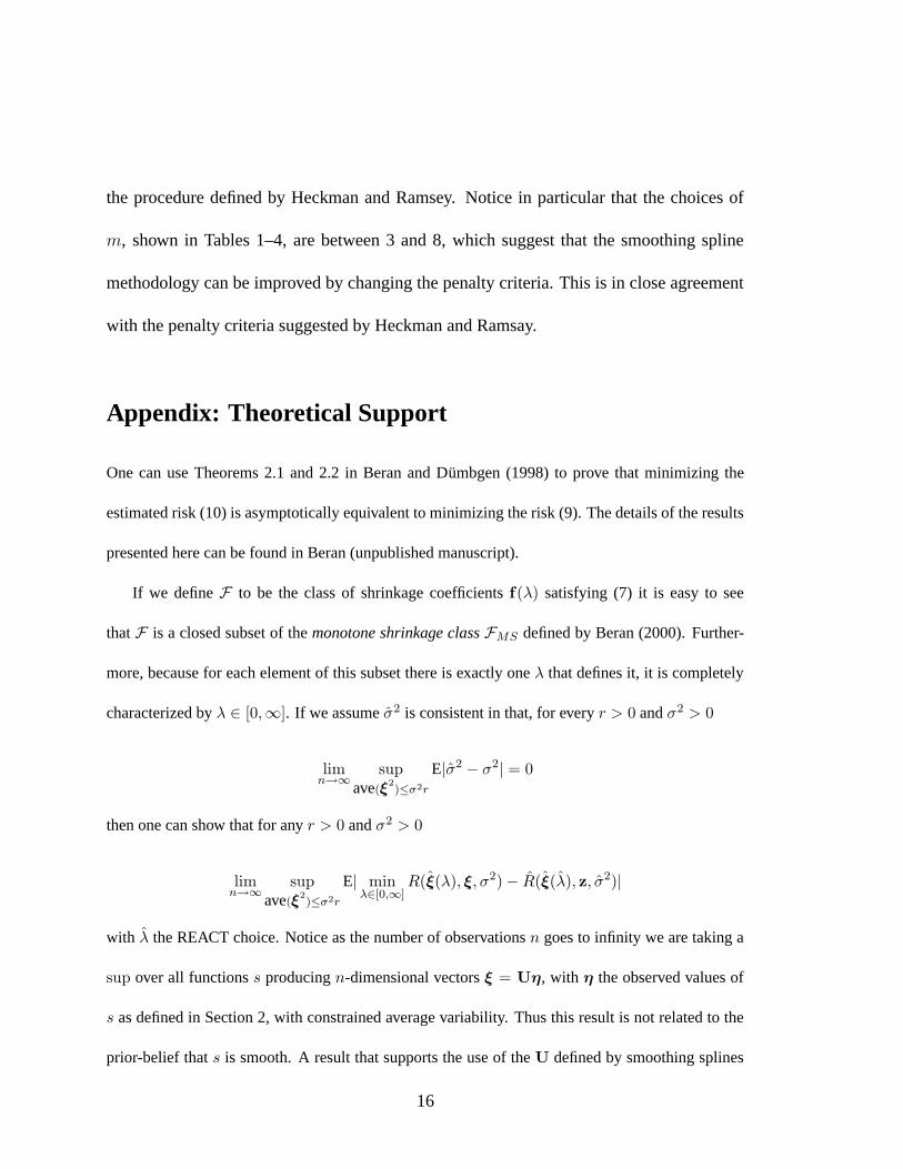
Table 1: Comparison of the two procedures for function 1. The λ column shows the averageof the λs chosen over the 100 simulations. The MSE column shows the average of theEuclidean distances between η and η divided by σ2 and multiplied by 100. Finally, for eachcriteria except CV, the % column shows the number of times (out of the 100 simulations)that criteria beats the CV criteria in terms of Euclidean distance between η and η.

Experiment CV REACT REDACT GML REACTm REDACTmn, σ λ MSE λ MSE % λ MSE % λ MSE % λ m MSE % λ m MSE %50,0.025 10 0.74 19 0.8 22 5.4 0.8 56 0.13 1.5 5 0.12 5.4 0.74 47 0.24 5.7 0.73 6250,0.05 22 0.94 24 0.92 46 14 1 59 4.2 0.99 41 0.25 5.2 0.87 68 0.54 5.6 1 5850,0.1 55 1.2 41 1.2 63 32 1.3 49 14 1.2 50 14 4.5 1.2 59 2.8 4.8 1.4 4750,0.5 460 2.1 280 2.1 49 270 2.3 45 230 1.9 58 1000 4.7 2.1 47 600 4.7 2.6 42100,0.025 6.5 0.56 6.7 0.53 57 3.8 0.55 56 0 1.6 0 0.57 4.2 0.53 56 0.86 4.3 0.58 49100,0.05 14 0.7 12 0.68 65 9.7 0.7 60 2.4 0.88 32 4.6 4.5 0.68 57 1.5 4.7 0.82 46100,0.1 34 0.89 22 0.89 56 21 0.91 49 7.8 0.89 43 57 4 0.91 56 48 4.2 1.2 47100,0.5 330 1.7 200 1.7 47 190 1.8 51 130 1.6 64 750 4.6 1.7 50 670 4.7 2 44250,0.025 4 0.38 2.7 0.36 61 2.3 0.36 64 0.15 1.3 3 1.3 3.3 0.36 69 1.5 3.3 0.36 61250,0.05 8.6 0.44 6 0.44 59 5.7 0.44 60 1.2 0.48 23 7 3.8 0.44 58 5.6 3.8 0.45 53250,0.1 19 0.57 13 0.57 55 13 0.57 58 3.9 0.59 34 20 4.1 0.56 58 20 4.3 0.56 58250,1 410 2 230 2.1 44 240 2.1 47 190 1.8 68 750 4.1 2.1 48 720 4.2 2.9 48

Table 2: Like table 1, but for function 2.Experiment CV REACT REDACT GML REACTm REDACTmn, σ λ MSE λ MSE % λ MSE % λ MSE % λ m MSE % λ m MSE %50,0.025 29 0.6 45 0.63 33 20 0.62 51 1.7 0.95 15 0.13 7.4 0.42 94 0.12 7.5 0.43 9150,0.05 49 0.77 53 0.75 60 35 0.82 47 5.9 0.88 17 0.35 6.5 0.59 90 0.58 6.7 0.63 8350,0.1 110 1.1 85 1.1 52 74 1.2 52 20 1.1 44 43 6 0.97 72 11 6.1 1.4 6550,0.5 1400 2.3 380 2.3 53 350 2.5 46 280 1.9 67 820 5 2.1 63 520 5.1 2.8 54100,0.025 22 0.45 20 0.44 55 14 0.45 53 0 1.6 0 0.75 6.4 0.33 94 0.69 6.5 0.41 84100,0.05 40 0.6 32 0.59 51 29 0.6 56 3.8 0.67 26 11 6 0.5 88 8.8 6.1 0.6 81100,0.1 70 0.76 49 0.8 49 47 0.83 45 11 0.85 28 86 5.4 0.75 58 48 5.6 1 55100,0.5 370 1.6 230 1.8 47 220 2 44 150 1.6 63 830 4.9 1.7 50 620 4.9 2.5 46250,0.025 14 0.28 11 0.27 54 10 0.27 55 0 1.6 0 0.95 5.6 0.22 90 0.82 5.7 0.22 87250,0.05 27 0.37 19 0.37 52 19 0.37 51 1.6 0.99 15 11 5.5 0.32 73 11 5.6 0.33 70250,0.1 52 0.49 37 0.5 55 37 0.5 53 5.7 0.56 21 35 5.7 0.45 72 35 5.8 0.45 72250,1 530 2 290 2.2 57 290 2.5 51 230 1.7 60 780 4.9 2.1 60 770 5.1 2.8 59

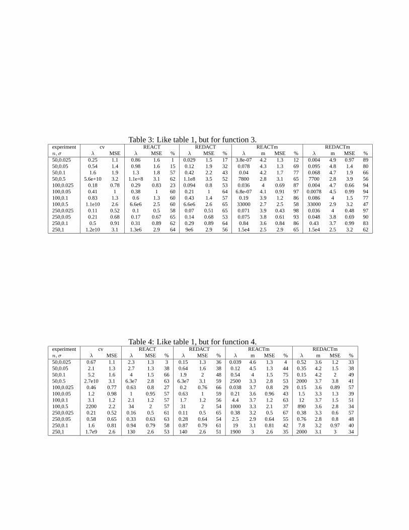
Table 3: Like table 1, but for function 3.experiment cv REACT REDACT REACTm REDACTmn, σ λ MSE λ MSE % λ MSE % λ m MSE % λ m MSE %50,0.025 0.25 1.1 0.86 1.6 1 0.029 1.5 17 3.8e-07 4.2 1.3 12 0.004 4.9 0.97 8950,0.05 0.54 1.4 0.98 1.6 15 0.12 1.9 32 0.078 4.3 1.3 69 0.095 4.8 1.4 8050,0.1 1.6 1.9 1.3 1.8 57 0.42 2.2 43 0.04 4.2 1.7 77 0.068 4.7 1.9 6650,0.5 5.6e+10 3.2 1.1e+8 3.1 62 1.1e8 3.5 52 7800 2.8 3.1 65 7700 2.8 3.9 56100,0.025 0.18 0.78 0.29 0.83 23 0.094 0.8 53 0.036 4 0.69 87 0.004 4.7 0.66 94100,0.05 0.41 1 0.38 1 60 0.21 1 64 6.8e-07 4.1 0.91 97 0.0078 4.5 0.99 94100,0.1 0.83 1.3 0.6 1.3 60 0.43 1.4 57 0.19 3.9 1.2 86 0.086 4 1.5 77100,0.5 1.1e10 2.6 6.6e6 2.5 60 6.6e6 2.6 65 33000 2.7 2.5 58 33000 2.9 3.2 47250,0.025 0.11 0.52 0.1 0.5 58 0.07 0.51 65 0.071 3.9 0.43 98 0.036 4 0.48 97250,0.05 0.21 0.68 0.17 0.67 65 0.14 0.68 53 0.075 3.8 0.61 93 0.048 3.8 0.69 90250,0.1 0.5 0.91 0.31 0.89 62 0.29 0.89 64 0.84 3.6 0.84 86 0.43 3.7 0.99 83250,1 1.2e10 3.1 1.3e6 2.9 64 9e6 2.9 56 1.5e4 2.5 2.9 65 1.5e4 2.5 3.2 62

Table 4: Like table 1, but for function 4.experiment cv REACT REDACT REACTm REDACTmn, σ λ MSE λ MSE % λ MSE % λ m MSE % λ m MSE %50,0.025 0.67 1.1 2.3 1.3 3 0.15 1.3 36 0.039 4.6 1.3 4 0.52 3.6 1.2 3350,0.05 2.1 1.3 2.7 1.3 38 0.64 1.6 38 0.12 4.5 1.3 44 0.35 4.2 1.5 3850,0.1 5.2 1.6 4 1.5 66 1.9 2 48 0.54 4 1.5 75 0.15 4.2 2 4950,0.5 2.7e10 3.1 6.3e7 2.8 63 6.3e7 3.1 59 2500 3.3 2.8 53 2000 3.7 3.8 41100,0.025 0.46 0.77 0.63 0.8 27 0.2 0.76 66 0.038 3.7 0.8 29 0.15 3.6 0.89 57100,0.05 1.2 0.98 1 0.95 57 0.63 1 59 0.21 3.6 0.96 43 1.5 3.3 1.3 39100,0.1 3.1 1.2 2.1 1.2 57 1.7 1.2 56 4.4 3.7 1.2 63 12 3.7 1.5 51100,0.5 2200 2.2 34 2 57 31 2 54 1000 3.3 2.1 37 890 3.6 2.8 34250,0.025 0.21 0.52 0.16 0.5 61 0.11 0.5 65 0.38 3.2 0.5 67 0.38 3.3 0.6 57250,0.05 0.58 0.65 0.33 0.63 63 0.28 0.64 54 2.5 2.9 0.64 55 0.76 2.8 0.8 48250,0.1 1.6 0.81 0.94 0.79 58 0.87 0.79 61 19 3.1 0.81 42 7.8 3.2 0.97 40250,1 1.7e9 2.6 130 2.6 53 140 2.6 51 1900 3 2.6 35 2000 3.1 3 34

•• • • •

•

•

•

•

•

• •

•

• • • • • •

•

•

•

• • • • • • • • •

•

•

•

•

• •

•

• •

• •

• • •

•

•

•

• ••

••

•

•

•

•

•• • •

•

•

•

• • • •

•

• • •

•

• • • • • • • • • • •

•

• • •

•

• • • • • • •

•

•

•

•

Empirical and Estimated shrinkage coefficients

j

g_j

0 10 20 30 40 50

0.0

0.2

0.4

0.6

0.8

1.0

a

aaaa

a

a

a

aa

aa

a

a

aa

aa

a

aaa

a

aa

aa

a

a

a

a

aa

aa

aa

a

aa

aaa

a

aa

a

a

aaa

Weights used

j

a_j^

2 an

d b_

j^2

0 10 20 30 40 50

10^-

510

^-3

10^-

110

^1

b

b

b

b

b

bb

bb

bb

b

b

b

b

b

bb

bb

b

b

b

bb

bb

b

b

bb

b

b

b

b

b

b

b

b

b

b

b

bbb

b

b

b

b

Figure 1: The first plot shows the empirical shrinkage coefficients g for a Monte Carlorealization of (eq0) with n = 100, σ = 0.05, and s is function 3. The solid line showsthe fitted shrinkage coefficients using the REACT choice for λ. The dashed line showsthe fitted shrinkage coefficients when both λ and m are obtained using the REACTcriterion. The second plot shows the weights ais and bjs used in the weighted leastsquares equation used to obtain the REACT criterion.

Function 1

x

s(t)

0.0 0.4 0.8

0.0

0.2

0.4

0.6

0.8

1.0

Function 2

x

s(t)

0.0 0.4 0.8

0.0

0.2

0.4

0.6

0.8

1.0

Function 3

x

s(t)

0.0 0.4 0.8

0.0

0.2

0.4

0.6

0.8

1.0

Function 4

x

s(t)

0.0 0.4 0.8

0.0

0.2

0.4

0.6

0.8

1.0

Figure 2: These are plots of the 4 functions used in the simulation.

•

•

••

•

•

•

•

•

•

•

•

•

•

•

•

•

•

•

•

•

•

•

•

••

•

•

•

•

•

•

•

•

•

••

•

•

•

•

•

•

•

•

•

•

•

x

y

0.0 0.2 0.4 0.6 0.8 1.0

-10

1

REACTCVGML

Figure 3: The points are the 48 measurements of activity taken every 30 minutes during oneday for an AKR mice, The grey region denotes the unbiased estimate obtained using themean of the 47 days we have observations from surrounded by pointwise standard errors.The solid line is the estimate obtained using the REACT criterion. The 2 dotted lines arethe estimates obtained with the CV and GML criteria.