choice of anchor tests in equating - educational … introduction the non-equivalent groups with...

Choice of Anchor Test in Equating

November 2006 RR-06-35

ResearchReport

Sandip Sinharay

Paul Holland

Research & Development

Choice of Anchor Test in Equating

Sandip Sinharay and Paul Holland

ETS, Princeton, NJ

November 2006

As part of its educational and social mission and in fulfilling the organization's nonprofit charter

and bylaws, ETS has and continues to learn from and also to lead research that furthers

educational and measurement research to advance quality and equity in education and assessment

for all users of the organization's products and services.

ETS Research Reports provide preliminary and limited dissemination of ETS research prior to

publication. To obtain a PDF or a print copy of a report, please visit:

http://www.ets.org/research/contact.html

Copyright © 2006 by Educational Testing Service. All rights reserved.

ETS and the ETS logo are registered trademarks of Educational Testing Service (ETS).

SAT is a registered trademark of the College Board.

Abstract

It is a widely held belief that anchor tests should be miniature versions (i.e., minitests),

with respect to content and statistical characteristics of the tests being equated. This

paper examines the foundations for this belief. It examines the requirement of statistical

representativeness of anchor tests that are content representative. The equating performance

of several types of anchor tests, including those having statistical characteristics that differ

from those of the tests being equated, is examined through several simulation studies and

a real data example. Anchor tests with a spread of item difficulties less than that of a

total test seem to perform as well as a minitest with respect to equating bias and equating

standard error. Hence, the results demonstrate that requiring an anchor test to mimic the

statistical characteristics of the total test may be too restrictive and need not be optimal.

As a side benefit, this paper also provides a comparison of the equating performance of

post-stratification equating and chain equipercentile equating.

Key words: Chain equating, correlation coefficient, minitest, NEAT design, post-

stratification equating

i

1 Introduction

The non-equivalent groups with anchor test (NEAT) design is one of the most

flexible tools available for equating tests (e.g., Angoff, 1971; Kolen & Brennan, 2004;

Livingston, 2004; Petersen, Kolen, & Hoover, 1989; Petersen, Marco, & Stewart, 1982).

The NEAT design deals with two nonequivalent groups of examinees and an anchor test.

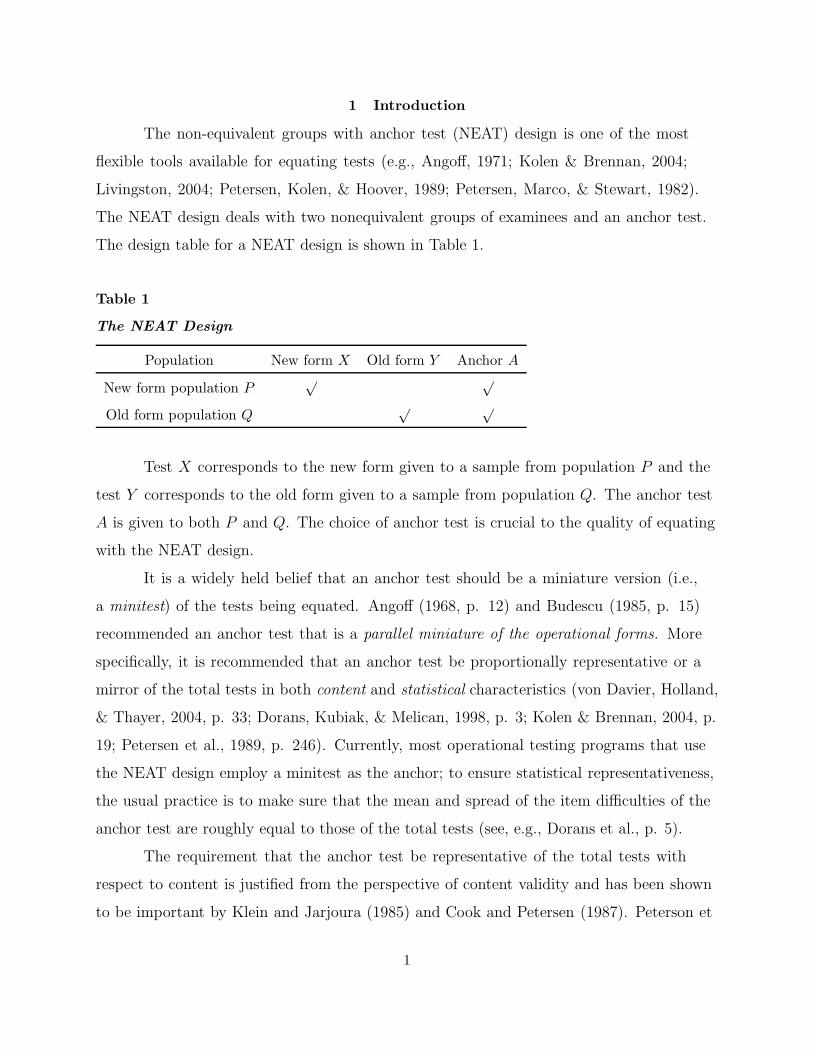
The design table for a NEAT design is shown in Table 1.

Table 1

The NEAT Design

Population New form X Old form Y Anchor A

New form population P√ √

Old form population Q√ √

Test X corresponds to the new form given to a sample from population P and the

test Y corresponds to the old form given to a sample from population Q. The anchor test

A is given to both P and Q. The choice of anchor test is crucial to the quality of equating

with the NEAT design.

It is a widely held belief that an anchor test should be a miniature version (i.e.,

a minitest) of the tests being equated. Angoff (1968, p. 12) and Budescu (1985, p. 15)

recommended an anchor test that is a parallel miniature of the operational forms. More

specifically, it is recommended that an anchor test be proportionally representative or a

mirror of the total tests in both content and statistical characteristics (von Davier, Holland,

& Thayer, 2004, p. 33; Dorans, Kubiak, & Melican, 1998, p. 3; Kolen & Brennan, 2004, p.

19; Petersen et al., 1989, p. 246). Currently, most operational testing programs that use

the NEAT design employ a minitest as the anchor; to ensure statistical representativeness,

the usual practice is to make sure that the mean and spread of the item difficulties of the

anchor test are roughly equal to those of the total tests (see, e.g., Dorans et al., p. 5).

The requirement that the anchor test be representative of the total tests with

respect to content is justified from the perspective of content validity and has been shown

to be important by Klein and Jarjoura (1985) and Cook and Petersen (1987). Peterson et

1

al. (1982) demonstrated the importance of having the mean difficulty of the anchor tests

close to that of the total tests. We also acknowledge the importance of these two aspects

of an anchor test. However, the literature does not offer any proof of the superiority of an

anchor test for which the spread of the item difficulties is representative of the total tests.

Furthermore, a minitest has to include very difficult or very easy items to ensure adequate

spread of item difficulties, which can be problematic as such items are usually scarce. An

anchor test that relaxes the requirement on the spread of the item difficulties could be more

operationally convenient.

This paper focuses on anchor tests that

• are content representative

• have the same mean difficulty as the total test

• have spread of item difficulties not equal to that of the total tests

Operationally, such an anchor can be constructed exactly in the same manner as the

minitests except that there is no need to worry about the spread of the item difficulties.

Because items with medium difficulty are usually more abundant, the most operationally

convenient strategy with such a procedure will be to include several medium-difficulty items

in the anchor test. This will lead to the anchor test having less spread of item difficulties

than that of the total tests.

To demonstrate the adequate performance of anchor tests with spread of item

difficulties less than that of the minitest, Sinharay and Holland (2006) considered anchor

tests referred to as miditest (when the anchor test has zero as the spread of item difficulties)

and semi-miditest (when the anchor test has a spread of item difficulties between zero and

that of the total tests). These anchor tests, especially the semi-miditest, will often be easier

to construct operationally than the minitests because there will be no need to include very

difficult or very easy items in these. Sinharay and Holland cited several works that suggest

that the miditest will be satisfactory with respect to psychometric properties like reliability

and validity. The next step is to examine how these anchor tests perform compared to the

minitests.

2

Sinharay and Holland (2006) showed that the miditests and semi-miditests have

slightly higher anchor-test-to-total-test correlations than the minitests, using a number of

simulation studies and a real data example. As higher anchor-test-to-total-test correlations

are believed to lead to better equating (Angoff, 1971, p. 577; Dorans et al., 1998; Petersen

et al., 1989, p. 246, etc.), the findings of Sinharay and Holland suggest that a minitest

may not be the optimum anchor test and indicate the need for a direct comparison

of the equating performance of minitests versus midi- and semi-miditests. Hence, the

present paper compares the equating performance of minitests versus that of midi- and

semi-miditests through a series of simulation studies and a pseudo-data example.

The next section compares the minitests versus the other anchor tests for a simple

equating design. The following two sections compare the equating performance of the

minitest and the other anchor tests in the context of NEAT design using data simulated

from unidimensional and multidimensional item response theory (IRT) models. The

penultimate section describes similar results for a pseudo-data example. The last section

provides discussion and conclusions.

2 Comparison of Minitests and Other Anchor Tests for a Simple Equating Design

Consider the simple case of a random groups design with anchor test ( Angoff, 1971;

Kolen & Brennan, 2004; Lord, 1950) in which randomly equivalent groups of examinees are

administered one of two tests that include an anchor test. Denote by X and Y the tests

to be equated and the anchor test by A. Under the assumptions that (a) the populations

taking tests X and Y are randomly equivalent, (b) scores on X and A, and on Y and A are

bivariate normally distributed, (c) the correlation between scores in X and A is equal to

that between scores in Y and A, and (d) sample sizes for examinees taking the old and new

forms are equal, Lord showed that the square of the standard error of equating (SEE) at

any value xi of scores in test X can be approximated as

Var(lY (xi)) ≈σ2

Y

N

[2(1 − ρ2

XA) + (1 − ρ4XA)

(xi − µX

σX

)2]

, (1)

where the symbols have their usual meanings. Equation 1 shows that as the anchor-test-

to-total-test correlation ρXA increases, the SEE decreases (a phenomenon mentioned by

3

0 20 40 60 80 100

0.1

0.2

0.3

0.4

0.5

0.6

Raw score

SE

E

MiniSemi−midi

Figure 1. Standard error of equating (SEE) for the miditest and minitest for the

common-item, random-groups design.

Budescu, 1985, p. 15). Therefore, higher correlations between X and A will result in lower

SEEs in this case. This basic fact emphasizes the importance of the results of Sinharay and

Holland (2006), which focused only on ρXA as a surrogate for the more detailed study of

equating in the present paper.

Sinharay and Holland (2006) considered a basic skills test that had 6,489 examinees

and 110 multiple choice items. They used the operational 34-item internal anchor test as

a minitest. A semi-miditest was formed on the basis of the item difficulties. For the test

data set, N = 6489, µX = 77.5, σX = 10.8, and the values of ρXA were 0.875 and 0.893

for the minitest and the semi-miditest, respectively. The graphs of the SEEs, computed

using the above mentioned values and under the additional assumptions that σY = σX and

ρXA = ρY A, are shown in Figure 1 to illustrate Equation 1.

In Figure 1, the SEE for the semi-miditest is always less than that for the minitest.

The percentage reduction in SEE for the semi-miditest ranges from 6% to 7%.

No result as simple as Equation 1 is found for the other popular equating designs,

4

especially for the NEAT design. Furthermore, in addition to sampling variability (or SEE),

it is also important to examine the other major type of equating error: the systematic

error or equating bias (Kolen & Brennan, 2004, p. 231). There are no general results for

measuring equating bias. Hence, the next section reports the results of a detailed simulation

study under a NEAT design that was performed to investigate both equating bias and

variability under several conditions.

3 Simulations Under a NEAT Design From a Univariate IRT Model

3.1 Simulation Design

Factors controlled in the simulation. We varied the following factors in the

simulations:

1. Test length. X and Y are always of equal length that is one of the values 45, 60,

and 78, to emulate three operational tests: (a) a basic skills test, (b) the mathematics

section of an admissions test, and (c) the verbal section of the same admissions test.

The factor that we henceforth denote by test length refers to more than simply the

length of the tests to be equated. Each test length has its own set of item parameters

that was created to emulate those of the operational test data set on which it is based

(see below). Moreover, the length of the anchor test for each test length is different as

indicated in Point 5, below. For this reason we italicize test length.

2. Sample size. We used three sizes: small (100), medium (500), and large (5,000). The

sample sizes for P and Q are equal.

3. The difference in the mean ability (denoted as ∆a) of the two examinee populations P

and Q. Four values were used: −0.2, 0, 0.2, and 0.4.

4. The difference in the mean difficulty (denoted as ∆d) of the two tests X and Y . Five

values were used: −0.2, 0, 0.1, 0.2, and 0.5.

5. The anchor test. We constructed a minitest, a semi-miditest, and a miditest by varying

the standard deviation (SD) of the generating difficult parameters. The SD of the

difficulty parameters of the minitest, the semi-miditest, and the miditest were assumed

5

to be, respectively, 100%, 50%, and 10% of the SD of the difficulty of the total tests.

The anchor test has 20 items for the 45-item basic skills test and is the same length as

the operational administrations of the two admissions tests—35 items for the 78-item

test and 25 items for the 60-item test. The average difficulty of the anchor tests was

always centered at the average difficulty level of Y , the old test form.1

6. The equating method. To make sure that our conclusions do not depend on the equating

method, we used two equating methods, the post-stratification equipercentile (PSE)

and chain equipercentile equating (CE) methods. While applying the PSE method,

the synthetic population was formed by placing equal weights on P and Q.

The values for the above six factors were chosen after examining data from

several operational tests. Generating item parameters for the total and anchor tests. The

two-parameter logistic (2PL) model, with the item response function (IRF),

exp[ai(θ − bi)]

1 + exp[ai(θ − bi)],

where the symbols have their usual meanings, was fitted to a data set from each of the

above mentioned three operational tests to obtain marginal maximum likelihood estimates

of the item parameters under a N (0, 1) ability distribution. These three sets of item

parameter estimates were used as generating item parameters of the three Y tests. Then,

a bivariate normal distribution D was fitted to the estimated log(a)’s and b’s for each Y

test—this involved computing the mean and variance of the estimated log(a)’s and b’s and

the correlation among them. The generating item parameters for each X test were drawn

from the respective fitted bivariate normal distribution D. Then the difficulty parameters

for X were all increased by the amount ∆d to ensure that the difference in mean difficulty

of X and Y is equal to ∆d. The generating item parameters for the anchor tests were also

drawn using the fitted distribution D. The generating item parameters of the minitest were

drawn from the distribution D as is. The item parameters of the semi-miditest and the

miditest were generated from a distribution that is the same as D except for the SD of

the difficulties, which was set to one half and one tenth, respectively, of the corresponding

quantity in D. Note that the generating a parameters were obtained, whenever applicable,

6

by taking an exponential transformation of the generated log(a)s. The generating item

parameters for the X test, Y test, and the anchor tests were the same for all R replications

under a simulation condition. For any combination of a test length, ∆a, and ∆d, the

population equipercentile equating function (PEEF), described shortly, is computed and used

as the criterion. The steps in the simulation. For each simulation condition (determined

by a test length, sample size, ∆a, and ∆d), the generating item parameters of the Y test

were the same as the estimated item parameters from the corresponding real data, and the

generating item parameters of the X test and the anchor tests were randomly drawn (as

described earlier) once, and then M = 1, 000 replications were performed. Each replication

involved the following three steps:

1. Generate the ability parameters θ for the populations P and Q from gP (θ) = N (∆a, 1)

and gQ(θ) = N (0, 1), respectively.

2. Simulate scores on X in P , Y in Q, and those on mini-, midi-, and semi-miditests for

both P and Q from a 2PL model using the draws of θ from Step 1, the fixed item

parameters for Y , and the generated item parameters for X and the anchor tests.

3. Perform six equatings using the scores of X in P , Y in Q, and those of the mini-,

midi-, and semi-miditest in P and Q. One equating is done for each combination of

one (of the three) anchor test and one (either PSE or CE) equating method. Each of

these equatings involved (a) presmoothing the observed test-anchor test bivariate raw

score distribution using a loglinear model (Holland & Thayer, 2000) that preserved

the first five univariate moments and a crossproduct moment (increasing the number

of moments did not affect the results substantially), and (b) equipercentile equating

with linear interpolation (e.g., Kolen & Brennan, 2004) to continuize the discrete score

distribution.

Computation of the population equipercentile equating function. The PEEF for any

combination of a test length, ∆a, and ∆d was the single-group equipercentile equating

of X to Y using the true raw score distribution of X and Y in a synthetic population

T that places equal weights on P and Q. We used the iterative approach of Lord and

Wingersky (1984) to obtain P (X = x|θ), the probability of obtaining a raw score of X = x

7

by an examinee with ability θ. This required the values of the item parameters and we used

the generating item parameters. Once P (X = x|θ) is computed, r(x), the probability of a

raw score of x on test X in population T is obtained by numerical integration as

r(x) =

∫

θ

P (X = x|θ)gT (θ)dθ, (2)

where we used gT (θ) = 0.5gP (θ) + 0.5gQ(θ). The same approach provided us with s(y), the

probability of a raw score of y on test Y in population T . The true raw score distributions

r(x) and s(y), both discrete distributions, are then continuized using linear interpolation

(e.g., Kolen & Brennan, 2004). Let us denote the corresponding continuized cumulative

distributions as R(x) and S(y), respectively. The PEEF is then obtained as S−1(R(x)).

The PEEF is the same for each replication and sample size, but varies with test length, ∆a,

and ∆d. The PEEF can be seen as the population value of the IRT observed score equating

(e.g., Kolen & Brennan, 2004) using linear interpolation as the continuization method.

Computation of the performance criteria: Equating bias, SD, and RMSE. After the

equating results from the M replications are obtained, we compare the anchor tests using

bias (a measure of systematic error in equating) and SD (a measure of random error in

equating) as performance criteria. For a simulation condition, let ei(x) be the equating

function in the i-th replication providing the transformation of a raw score point x in X to

the raw score scale of Y . Suppose e(x) denotes the corresponding PEEF. The bias at score

point x is obtained as

Bias(x) =1

M

M∑

i=1

[ei(x) − e(x)] = ¯e(x) − e(x), where ¯e(x) =1

M

M∑

i=1

ei(x),

and the corresponding SD is obtained as

SD(x) =

{1

M

M∑

i=1

[ei(x) − ¯e(x)]2

} 1

2

·

The corresponding root mean squared error (RMSE) can be computed as

RMSE(x) =

{1

M

M∑

i=1

[ei(x) − e(x)]2

} 1

2

·

It can be shown that

[RMSE(x)]2 = [SD(x)]2 + [Bias(x)]2 ,

8

that is, the RMSE combines information from the random and systematic error.

As overall summary measures for each simulation case, we compute the weighted

average of bias,∑

x r(x)Bias(x), the weighted average of SD,√∑

x r(x)SD2(x), and the

weighted average of RMSE,√∑

x r(x)RMSE2(x), where r(x) is defined in Equation 2.

How realistic are our simulations? To have wide implications, it is important that these

simulations produce test data that adequately reflect reality. Hence, we used real data as

much as possible in our simulations from a unidimensional IRT model. Further, Davey,

Nering, and Thompson (1997, p. 7) reported that simulation under an unidimensional IRT

model reproduces the raw score distribution of real item response data quite adequately.

The data sets simulated in our study were found to adequately reproduce the raw score

distributions of the three operational data sets considered. Because the observed score

equating functions are completely determined by the raw score distribution, our simulations

are realistic for our purpose. We chose the 2PL model as the data generating model because

Haberman (2006) demonstrated that it describes real test data as well as the 3PL model.

Although we generate data from an IRT model in order to conveniently manipulate several

factors (most importantly, the item difficulties for the anchor tests) in the simulation, we

are not fitting an IRT model here. Hence, issues of poor IRT model fit are mostly irrelevant

to this study.

3.2 Results

Tables 2 to 7 contain the weighted averages of bias, SD, and RMSE for the several

simulation conditions.

In Tables 2 to 7, each vertical cell of three values corresponds to a simulation

condition. The three numbers in each cell correspond, respectively, to the minitest, the

semi-miditest, and the miditest. The appendix includes Figures A1 to A4 showing the

equating bias, SD, and RMSE for the CE method for several simulation cases.

Figure 2 shows the estimated equating function (EEF) and PEEF for 1 randomly

chosen replication and the differences between the EEF and the PEEF for a minitest and

semi-miditest for 10 randomly chosen replications for CE and PSE for the simulation case

with 45 items, 5,000 examinees, ∆a=0.4, and ∆d=0.5.

9

Table 2Bias (×100) for the Different Simulation Conditions: PSE Method

No. ∆d Number of examinees

of 100 500 5,000

items ∆a =−0.2 0.0 0.2 0.4 −0.2 0.0 0.2 0.4 −0.2 0.0 0.2 0.4

45 0.0 44 00 −45 −91 42 −01 −45 −88 43 00 −43 −87

43 01 −43 −87 42 00 −42 −84 42 00 −41 −83

42 01 −41 −83 39 00 −40 −79 40 00 −39 −78

0.2 42 −02 −47 −91 42 −01 −45 −88 43 00 −44 −87

41 −01 −44 −88 42 00 −42 −84 42 00 −42 −83

35 −05 −46 −86 39 −01 −40 −79 39 00 −40 −78

0.5 44 −02 −47 −91 42 −01 −44 −88 43 00 −44 −87

45 −01 −45 −87 42 00 −42 −84 42 00 −42 −83

34 −04 −45 −86 39 −01 −40 −79 39 00 −40 −79

60 0.0 32 −04 −41 −79 34 −01 −36 −72 35 00 −35 −71

30 03 −26 −56 27 01 −27 −56 27 00 −27 −55

29 01 −29 −59 29 02 −26 −55 27 00 −28 −57

0.2 32 −04 −41 −79 34 −01 −36 −72 34 00 −35 −71

31 03 −26 −56 27 00 −27 −56 27 00 −27 −56

29 01 −28 −60 29 02 −26 −56 27 00 −28 −57

0.5 33 −04 −41 −79 34 −01 −36 −72 34 00 −36 −71

31 04 −25 −56 27 01 −27 −56 27 00 −27 −56

30 01 −27 −59 28 02 −26 −56 27 00 −28 −57

78 0.0 35 −05 −45 −86 35 −03 −41 −80 38 00 −38 −76

33 −02 −38 −74 32 −01 −35 −68 33 00 −33 −66

30 −04 −40 −75 30 −03 −36 −69 32 00 −33 −66

0.2 36 −04 −44 −86 35 −03 −41 −80 38 00 −38 −76

34 −01 −37 −75 32 −01 −35 −69 33 00 −33 −67

31 −04 −40 −76 30 −03 −36 −70 32 00 −33 −67

0.5 39 −01 −40 −80 38 00 −38 −77 38 01 −38 −76

32 −03 −37 −72 33 00 −33 −68 33 00 −33 −67

35 00 −33 −69 33 00 −32 −67 33 01 −32 −66

Note. The three numbers in each cell correspond to the minitest, the semi-miditest, and the

miditest, respectively.

10

Table 3Bias (×100) for the Different Simulation Conditions: CE Method


of 100 500 5,000

items ∆a =−0.2 0.0 0.2 0.4 −0.2 0.0 0.2 0.4 −0.2 0.0 0.2 0.4

45 0.0 13 −02 −16 −31 12 −01 −15 −29 13 00 −14 −27

12 00 −13 −29 12 00 −13 −25 13 00 −12 −24

12 00 −13 −26 10 −01 −11 −22 11 00 −11 −21

0.2 11 −03 −17 −31 12 −02 −15 −29 13 00 −14 −28

12 −01 −14 −28 12 00 −13 −25 13 00 −12 −24

04 −07 −18 −29 10 −01 −11 −22 11 00 −11 −22

0.5 14 −03 −17 −30 12 −01 −14 −29 12 00 −14 −28

17 −01 −15 −27 13 00 −12 −25 12 00 −12 −25

02 −06 −17 −29 10 −01 −10 −22 10 00 −11 −22

60 0.0 06 −06 −19 32 10 −02 −13 −25 11 00 −11 −23

09 02 −06 −15 07 00 −07 −15 07 00 −07 −15

07 −01 −09 −19 09 02 −06 −15 07 00 −08 −16

0.2 06 −06 −18 −32 10 −02 −13 −25 11 00 −12 −24

09 03 −06 −15 07 00 −08 −16 07 00 −07 −15

08 00 −09 −19 09 02 −06 −15 07 00 −08 −17

0.5 07 −06 −18 −31 10 −02 −13 −25 11 00 −12 −24

10 03 −05 −15 07 00 −08 −16 07 00 −07 −15

08 00 −08 −18 09 02 −06 −15 07 00 −08 −17

78 0.0 06 −05 −17 −28 07 −03 −14 −24 10 00 −11 −21

07 −02 −12 −20 07 −01 −09 −17 08 00 −07 −15

04 −05 −14 −22 05 −03 −11 −19 07 00 −08 −15

0.2 07 −04 −15 −28 07 −03 −14 −25 11 00 −11 −21

08 −01 −10 −20 07 −01 −09 −17 08 00 −07 −16

04 −04 −13 −23 05 −03 −11 −19 07 00 −08 −16

0.5 10 −02 −12 −23 11 00 −11 −22 12 01 −11 −22

06 −04 −12 −20 08 00 −08 −17 09 01 −08 −17

09 00 −08 −17 08 00 −08 −17 09 01 −08 −16



11

Table 4SD (×100) for the Different Simulation Conditions: PSE Method


of 100 500 5,000

items ∆a =−0.2 0.0 0.2 0.4 −0.2 0.0 0.2 0.4 −0.2 0.0 0.2 0.4

45 0.0 112 112 114 117 51 50 51 52 15 15 15 16

111 111 112 115 49 48 49 50 15 15 15 15

109 109 111 114 50 49 50 50 15 15 15 15

0.2 111 110 112 116 51 50 51 52 15 16 15 16

107 106 107 111 49 48 49 50 15 15 15 15

108 106 108 111 50 49 50 50 15 15 15 15

0.5 115 111 114 113 51 50 51 51 16 15 15 16

106 106 107 109 49 49 49 49 15 15 15 15

106 106 107 109 50 49 50 50 15 15 15 15

60 0.0 130 129 130 136 56 55 56 57 17 17 17 18

124 124 125 131 53 53 53 54 17 16 17 17

123 123 125 131 53 53 53 55 17 16 16 17

0.2 129 129 130 134 56 55 56 57 17 17 17 18

123 123 124 129 53 53 53 54 17 16 17 17

123 122 124 129 53 53 53 55 17 16 16 17

0.5 130 129 129 133 56 55 55 57 17 17 17 18

124 122 123 128 53 53 53 54 17 16 17 17

124 123 124 128 53 53 53 54 16 16 16 17

78 0.0 157 157 159 169 69 69 69 71 22 21 22 22

158 158 160 168 66 66 67 69 21 21 21 21

158 157 159 167 67 66 67 69 21 21 21 22

0.2 147 147 151 159 65 65 65 68 21 20 21 21

149 149 154 161 63 63 64 67 20 20 20 21

150 149 154 161 63 63 64 67 20 20 21 22

0.5 149 148 160 166 69 68 68 69 21 21 21 21

144 143 155 161 68 67 67 68 21 20 21 21

143 143 154 162 68 67 67 69 21 21 21 21



12

Table 5SD (×100) for the Different Simulation Conditions: CE Method


of 100 500 5,000

items ∆a =−0.2 0.0 0.2 0.4 −0.2 0.0 0.2 0.4 −0.2 0.0 0.2 0.4

45 0.0 132 131 132 135 59 59 59 60 18 18 18 18

130 129 129 132 57 56 56 57 18 18 18 18

128 128 130 132 58 58 58 59 18 18 18 18

0.2 127 127 128 131 59 59 59 60 18 18 18 19

123 122 123 125 57 56 56 57 18 18 18 18

124 122 124 127 58 58 58 59 18 18 18 18

0.5 132 127 128 129 59 58 59 60 18 18 18 19

120 122 120 124 57 56 56 57 18 18 18 18

120 122 120 124 58 57 58 58 18 18 18 18

60 0.0 142 140 141 146 61 60 61 63 19 19 19 19

138 137 138 143 59 58 59 60 18 18 18 19

137 135 138 144 59 59 59 62 18 18 18 19

0.2 142 140 140 144 61 60 61 62 19 19 19 19

137 137 137 141 59 58 58 60 18 18 18 19

137 135 137 142 59 59 59 61 18 18 18 19

0.5 142 140 139 143 61 60 60 62 19 19 19 19

137 136 136 141 59 58 58 60 19 18 18 19

138 136 137 141 59 59 59 60 18 18 18 19

78 0.0 171 172 173 182 77 76 76 78 24 23 23 24

174 173 174 179 73 73 74 77 23 23 23 23

175 173 174 181 75 73 75 77 23 23 23 24

0.2 160 159 162 168 71 71 71 73 22 22 22 23

161 160 163 167 68 68 69 72 21 21 22 22

164 162 164 170 69 68 69 72 22 22 22 23

0.5 164 161 175 179 75 74 74 75 23 23 23 24

156 155 168 173 73 72 73 75 23 22 23 23

155 154 167 173 75 73 73 75 23 23 23 24



13

Table 6RMSE (×100) for the Different Simulation Conditions: PSE Method


of 100 500 5,000

items ∆a =−0.2 0.0 0.2 0.4 −0.2 0.0 0.2 0.4 −0.2 0.0 0.2 0.4

45 0.0 121 113 123 149 66 50 68 103 46 15 46 88

119 111 120 145 64 49 64 98 45 15 44 84

117 110 119 142 63 49 64 94 43 15 42 80

0.2 118 110 121 148 66 50 68 102 45 16 47 88

114 106 116 142 64 49 64 98 44 15 45 84

113 107 117 141 63 49 64 94 42 15 43 80

0.5 124 110 123 145 66 50 68 103 46 16 47 89

116 106 117 140 64 49 64 98 45 15 45 85

112 107 116 139 63 50 64 94 42 15 43 81

60 0.0 134 130 137 158 66 55 67 93 39 18 40 74

129 124 129 145 61 53 60 80 33 17 33 60

128 123 129 147 62 53 60 82 34 17 35 64

0.2 134 129 137 157 66 55 67 93 39 18 40 74

127 124 128 143 60 53 61 80 32 17 34 61

127 123 128 145 61 53 61 82 33 17 35 64

0.5 135 129 136 156 65 56 67 93 39 18 41 75

128 123 128 142 60 53 61 80 32 18 35 62

129 124 129 144 61 54 62 82 33 19 36 65

78 0.0 161 158 167 191 78 69 81 107 44 22 44 79

162 159 166 186 74 67 76 99 40 21 40 71

161 158 166 187 74 66 77 100 40 21 40 72

0.2 152 147 158 182 74 65 77 105 43 21 44 80

154 150 160 181 71 63 74 99 39 20 40 73

154 150 161 183 71 63 75 100 39 20 40 73

0.5 154 148 166 186 79 69 79 105 44 22 44 80

148 144 161 179 76 67 76 98 39 22 41 73

148 144 160 179 76 68 76 98 40 23 41 72



14

Table 7RMSE (×100) for the Different Simulation Conditions: CE Method


of 100 500 5,000

items ∆a =−0.2 0.0 0.2 0.4 −0.2 0.0 0.2 0.4 −0.2 0.0 0.2 0.4

45 0.0 133 131 133 139 60 59 61 67 22 18 23 33

131 129 130 136 58 56 58 63 22 18 21 30

129 128 131 136 59 58 59 63 21 18 21 28

0.2 127 127 129 135 60 59 61 67 22 18 23 34

123 122 124 129 58 56 58 62 22 18 22 30

125 123 126 130 59 58 59 63 21 18 21 29

0.5 133 127 129 133 60 59 61 67 23 18 23 34

121 122 121 128 58 56 57 62 22 18 22 31

121 123 122 128 59 58 59 63 21 18 21 29

60 0.0 143 141 143 150 62 61 62 68 23 19 23 31

139 138 139 146 60 59 60 63 21 19 21 26

138 136 139 147 61 59 60 66 22 19 22 30

0.2 143 140 142 148 62 60 62 67 23 19 23 31

138 138 139 144 60 59 59 63 21 19 21 27

138 136 138 145 61 59 60 65 22 19 23 31

0.5 143 141 141 148 62 60 62 68 23 20 23 32

138 137 138 143 60 59 60 64 22 20 23 29

139 137 139 144 61 60 61 66 23 21 24 32

78 0.0 172 173 175 185 77 76 78 82 26 23 26 32

175 174 176 182 73 73 75 80 25 23 25 30

176 174 176 185 75 74 76 81 25 23 25 31

0.2 161 160 163 171 72 71 73 77 25 22 25 31

162 161 164 170 68 68 70 75 23 22 24 30

165 162 166 173 70 69 71 76 23 22 24 30

0.5 165 162 176 182 76 74 75 79 27 24 27 33

157 156 170 176 75 73 74 78 26 24 26 31

156 155 168 176 76 74 75 79 27 25 27 32



15

0 10 20 30 40

010

2030

40

CE

Raw Score

Equ

atin

g fu

nctio

n

TrueMiniSemi−midi

0 10 20 30 40−

3−

2−

10

12

3

CE

Raw Score

Diff

eren

ce

MiniSemi−midi

0 10 20 30 40

010

2030

40

PSE

Raw Score

Equ

atin

g fu

nctio

n

0 10 20 30 40

−3

−2

−1

01

23

PSE

Raw Score

Diff

eren

ce

Figure 2. Estimated and true equating functions for one randomly chosen replication(left panels) and the differences between estimated and true equating functions for 10randomly chosen replications (right panels) for CE and PSE for the 45-item test with5,000 examinees, ∆a=0.4, and ∆d=0.5.

16

Figure 2 also shows, for convenience, the 10th and 90th percentiles of the true score

distribution of X , using dotted vertical lines. The plot shows hardly any difference between

the minitest and semi-miditest.

The SD of the raw scores on the operational tests are 7.1, 10.1, and 12.8 for the

45-item test, 60-item test, and 78-item test, respectively. As in Sinharay and Holland (2006),

the average total-test-to-anchor-test correlation is highest for the miditest followed by

the semi-miditest, and then the minitest. For example, for the 78-item test, sample size

5,000, ∆d=0.5, and ∆a=0.4, the averages are 0.888, 0.885, and 0.877, respectively. While

examining the numbers in Tables 2 to 7, remember that a difference of 0.5 or more in the

raw score scale is usually a difference that matters (DTM), that is, only a difference more

than a DTM leads to different scaled scores (Dorans & Feigenbaum, 1994).

The tables (and the figures in the appendix) lead to the following conclusions:

• Effects on bias (Tables 2 and 3; Figures A1 to A8):

– Group difference ∆a has a substantial effect on bias. This finding agrees with

earlier research work such as Hanson and Beguin (2002) and common advice by

experts (e.g., Kolen & Brennan, 2004, p. 232) that any group difference leads

to systematic error. Absolute bias is small when ∆a = 0 and increases as |∆a|increases. This holds for both CE and PSE. The sign of ∆a does not matter much.

– Both CE and PSE are biased, but CE is always less biased than PSE.

– Anchor test type has a small but nearly consistent effect on bias. Midi- and

semimidi- anchor tests are usually less biased than minitests. This holds for both

CE and PSE.

– Test length has a small effect on bias. It is not monotone for PSE and the effect

is smaller for CE.

– Both ∆d and sample size have almost no effect on bias.

• Effects on SD (Tables 4 and 5; Figures A1 to A8):

– Sample size has a large effect on SD.

17

– Test length has a modest effect on SD for both CE and PSE. SD increases as test

length increases.

– PSE has slightly less SD than CE, especially for small sample size conditions.

– ∆a has a small effect on SD that is largest for PSE and small sample sizes.

– Anchor test type has a small effect on SD, favoring miditests over minitests, mostly

for the small sample size.

– ∆d has almost no effect on SD.

• Effects on RMSE (Tables 6 and 7; Figures A1 to A8):

– Sample size has a large effect on RMSE.

– ∆a has a modest effect on RMSE.

– Test length has a modest effect on RMSE. RMSE increases as test length increases.

– CE versus PSE interacts with sample size in its effect on RMSE. PSE is slightly

better for the small sample size, while CE is much better for the large sample size

and is slightly better for the intermediate sample size.

– Anchor test type has a small but nearly consistent effect on RMSE favoring

miditests and semi-miditests over minitests for both CE and PSE.

– ∆d has almost no effect on RMSE.

With respect to the focus of this study, the main conclusion is that the effect of the

type of anchor test consistently favors miditests and semi-miditests over minitests, but it

is small, much smaller than the effects of (a) CE versus PSE for bias, SD, and RMSE, (b)

sample size on SD and RMSE, (c) ∆a on bias and RMSE, or (d) test length on SD and

RMSE.

The results that the CE is better than PSE with respect to equating bias and worse

than PSE with respect to SD in our simulations augment the recent findings of Wang, Lee,

Brennan, and Kolen (2006), who compared the equating performance of PSE and CE.

While Wang et al. varied the SD of the ability distribution and we did not, our study has

the advantage that we presmoothed the data and varied the sample size and test difficulty

difference, something that Wang et al. did not.

18

4 Simulations Under NEAT Design From a Multivariate IRT Model

4.1 Simulation Design

We obtained a data set from a licensing test. Of the total 118 items in the test,

Items 1–29 are on language arts, 30–59 are on mathematics, 60–88 are on social studies, and

89–118 are on science. As each of these four content areas can be considered to measure a

different dimension, we fitted a four-dimensional IRT model (e.g., Reckase, 1997) with IRF

(1 + e−(a1iθ1+a2iθ2+a3iθ3+a4iθ4−bi))−1, θ = (θ1, θ2, θ3, θ4)′ ∼ N4 (µ = (0, 0, 0, 0)′, Σ) (3)

to the data set, with the symbols having the usual meanings. The diagonals of Σ are set

to 1 to ensure identifiability of the model parameters. For any item i, only one among a1i,

a2i, a3i, and a4i is assumed to be nonzero, depending on the item content (e.g., for an item

from the first content area, a1i is nonzero while a2i = a3i = a4i = 0), so that we deal with a

simple-structure multivariate IRT (MIRT) model.

The estimated item parameter values were used as generating item parameters

of test Y . A bivariate normal distribution D∗k was fitted to the log-slope and difficulty

parameter estimates corresponding to k-th content area, k = 1, 2, . . . 4. The generating

item parameters for k-th content area for X were randomly drawn from D∗k. Because we

are considering multivariate tests here, X can differ from Y in more complicated ways than

for the univariate tests. Then we manipulated the difficulty parameters of test X in the

following ways to consider several patterns of differences in difficulty between X and Y :

• No difference (denoted as N)—no manipulation.

• We added ∆d to the generating difficulty parameters for the first content area for X

(denoted as O because the difference between X and Y is in one dimension).

• We added ∆d to the generating difficulty parameters for the first and third content

areas for X (denoted as T because the difference is in two dimensions).

• We added ∆d to the generating difficulty parameters of each item in X (denoted as A

because the difference is in all dimensions).

• We added ∆d to the generating difficulty parameters for the first and third content

areas in X, but subtracted ∆d from the generating difficulty parameters for the second

19

and fourth content area (denoted as D because the difference is differential in the

dimensions).

We assume that the anchor test has 12, 13, 12, and 13 items for the four content

areas, respectively, leading to an anchor length of 50. The generating item parameters for

the k-th content area for the anchor tests were also randomly drawn from the respective

distribution D∗k. The generating item parameters of the minitest were randomly drawn

from the distribution D∗k as is. The generating item parameters of the semi-miditest and

the miditest were randomly drawn from a distribution that is the same as D∗k except for

the SD of the difficulties, which was set to one half and one tenth, respectively, of the

corresponding quantity in D∗k. The generating item parameters for the tests X and Y and

the anchor tests were the same for all R replications.

We used only a test length of 118 and a sample size of 5,000 for the multivariate

simulation. We let ∆a vary among the three values—0, 0.2, and 0.4—and ∆d among the

three values—0, 0.2, and 0.5. We used two anchor tests (a minitest and semi-miditest) and

the same two equating methods (CE and PSE) as in the univariate IRT simulation.

The steps in the simulation are the same as those for the univariate IRT simulation

except for the following three differences:

• The number of replications was 200 here to reduce computational time.

• The difference between the populations P and Q may be of a more complicated nature,

just like the difference between the tests X and Y . We used gQ(θ) = N3(0, Σ), where

Σ is the estimate obtained from fitting the model expressed in Equation 3 to the

operational test data set. We used gP (θ) = N3(µP , Σ), where µP , which quantifies

the difference between P and Q, was set to be one of the following: (a) µP = 0, that

is, no difference (N) between P and Q, (b) µP = (∆a, 0, 0, 0)′, that is, one dimension

is different (O), (c) µP = (∆a, 0, ∆a, 0)′, that is, the two dimensions are different

(T), (d) µP = (∆a, ∆a, ∆a, ∆a)′, that is, all dimensions are equally different (A), and

(5) µP = (∆a,−∆a, ∆a,−∆a)′, that is, differentially different (D). The fifth type of

difference, D, is similar to what was found in, for example, Klein and Jarjoura (1985;

see, e.g., Figures 2 and 3 in that paper).

20

• Application of Equation 2 to compute the true equating function here would have

required four-dimensional numerical integration. Hence, we took a different approach

to compute the true equating function. For each simulation condition, we generated

responses to both X and Y of huge examinee samples, of size 250,000, from P and

Q, and performed a single-group equipercentile equating (combining the samples from

P and Q) with linear interpolation. We repeated this computation several times with

different random seeds—negligible differences between the equating functions obtained

from these repetitions ensured that the above procedure provided us with the true

equating function with sufficient accuracy.

4.2 Results

Tables 8 and 9 show the RMSEs for PSE and CE for the several simulation

conditions. Under each simulation case, the RMSEs are shown for the minitest at the top

and for the semi-miditest at the bottom of a cell. The SDs (not shown) are very close for

all the simulation conditions and the differences between the RMSEs arise mainly because

of differences in the equating bias.

The factor that has the largest effect on the RMSE is the population difference. The

pattern of difference between the two populations also has substantial effect, with pattern

A associated with the largest values of RMSE. The differences in the tests appear to have

no effect on the RMSE.

With respect to the focus of this study, several conditions slightly favor the

semi-miditest while a few others slightly favor the minitest. However, the difference in

RMSE between the minitest and the semi-miditest is always small and far below the DTM,

even under conditions that are adverse to equating and worse than what is usually observed

operationally. Thus, there seems to be no practically significant difference in equating

performance of the two anchor tests.

The results regarding comparison of PSE versus CE, which may be of interest

because Wang et al. (2006) did not generate data from a MIRT model, are similar to

those from our univariate IRT simulation. The RMSE for PSE is mostly larger than CE

when the populations are different, the largest differences being observed when population

21

Table 8RMSE (×100) Multivariate Simulation Conditions for the CE Method for a118-Item Test and Sample Size of 5,000 for the High-Correlation Case

Population Test difference

difference N O T A D

Pattern ∆a ∆d=0 0.2 0.5 0.2 0.5 0.2 0.5 0.2 0.5

N 0.0 32 31 32 31 32 32 32 31 32

30 30 31 30 31 30 31 30 31

O 0.2 31 32 31 32 31 32 31 32 32

30 31 31 31 31 30 31 30 31

0.4 32 31 33 31 31 31 32 32 35

31 32 33 32 32 32 32 32 34

T 0.2 32 32 31 33 31 33 31 34 31

31 31 31 32 31 31 31 32 30

0.4 36 31 31 32 34 32 32 31 32

34 31 31 32 34 32 32 31 31

A 0.2 34 34 33 34 34 34 34 34 33

33 33 34 34 34 34 34 34 34

0.4 43 42 42 42 42 42 43 41 41

42 43 43 43 43 43 44 43 42

D 0.2 31 31 31 32 31 31 31 34 40

31 31 31 31 32 32 32 31 37

0.4 32 32 34 32 34 32 34 37 60

34 32 32 34 37 34 35 33 53

Note. The two numbers in each cell correspond to the minitest and the semi-miditest,

respectively.

difference is of the type A and ∆a = 0.4 (whereas CE leads to RMSEs ranging between

0.41 to 0.43, PSE leads to RMSEs ranging between 1.03 to 1.07). Interestingly, the PSE

performs slightly better than CE when the population difference is of the type D, even

when ∆a = 0.4. This finding somewhat contradicts the recommendation of Wang et al. (p.

15) that “. . . generally speaking, the frequency estimation method does produce more bias

22

Table 9RMSE (×100) for the Different Multivariate Simulation Conditions for the PSEMethod for a 118-Item Test and Sample Size of 5,000 for the High-Correlation Case

Population Test difference

difference N O T A D

Pattern ∆a ∆d=0 0.2 0.5 0.2 0.5 0.2 0.5 0.2 0.5

N 0.0 29 29 30 29 30 30 30 29 30

28 28 28 28 29 28 30 28 29

O 0.2 31 32 32 32 30 32 31 32 32

31 31 32 31 30 31 32 31 32

0.4 37 36 39 34 34 35 36 37 42

36 37 39 35 35 36 38 37 42

T 0.2 38 39 30 40 32 39 31 42 29

37 37 31 38 33 37 32 40 29

0.4 58 35 35 38 41 36 38 33 32

54 37 36 39 43 37 39 34 32

A 0.2 59 59 56 59 57 59 57 59 56

58 57 58 58 58 58 59 58 58

0.4 107 103 103 103 103 103 103 103 103

105 105 105 106 106 105 106 105 105

D 0.2 29 29 28 29 30 29 30 30 35

29 29 29 29 31 30 31 29 34

0.4 30 30 29 34 37 32 32 29 47

37 33 31 39 42 36 37 30 43

Note. The two numbers in each cell correspond to the minitest and the semi-miditest,

respectively.

than chained equipercentile method and the difference in bias increases as group differences

increase,” as the difference in bias seems to depend in a complicated manner on the type of

group difference. This can be a potential future research topic.

For the data set from the 118-item test, the estimated correlations between the

components of θ range between 0.73 to 0.89, which can be considered too high for the

23

test to be truly multidimensional. Hence, we repeated the simulations by considering

a variance matrix (between the components of θ) Σ∗ whose diagonals are the same as

those of Σ, but whose off-diagonals are readjusted to make each correlation implied by Σ∗

0.15 less than that implied by Σ. This brings down the correlations to values (between

0.58 and 0.74) that are high enough to be practical, but also low enough for the test

to be truly multidimensional. The results for these simulations are similar to those in

Tables 8 and 9 and are not reported. We also considered several content-nonrepresentative

anchor tests, but they had mostly large RMSEs, demonstrating the importance of content

representativeness of the anchor tests, and results are not reported for them. We also

repeated the above multivariate IRT simulation procedure using an admissions test data

set; we fitted a three-dimensional MIRT model as the test has three distinct item types;

the results were similar as above, that is, there was hardly any difference in the equating

performance of the minitest and the semi-miditest.

5 Pseudo-Data Example

It is not easy to compare a minitest versus a miditest or a semi-miditest in an

operational setting as almost all operational anchor tests are constructed to be minitests

following the above mentioned recommendations. However, a study by von Davier, Holland,

and Livingston (2005) allowed us to make the comparison even though study is rather

limited because of short test lengths and short anchor lengths. The study considered a

120-item test given to two populations P and Q of sizes 6,168 and 4,237, respectively. The

population Q has a higher average score (by about a quarter in SD-of-raw-score unit).

Two 44-item tests, X and Y , and three anchor tests that were minitests of 16, 20, and 24

items were constructed by partitioning the 120-item test. The 20-item anchor test was a

subset of the 24-item anchor test and the 16-item anchor test was a subset of the 20-item

anchor test. Test X was designed to be much easier (the difference being about 128% in

SD-of-raw-score unit) than test Y .

Of the total 120 items in the test, Items 1–30 were on language arts, 31–60 were on

mathematics, 61–90 were on social studies, and 91–120 are on science. As the minitest, we

used the 16-item anchor test in von Davier et al. (2005). There were not enough middle

24

difficulty items to choose a miditest. The semi-miditest was a subset of the 24-item anchor

test in von Davier et al. We ranked the six items within each of the four content areas in

the 24-item anchor test according to their difficulty (proportion correct); the four items that

ranked second to fifth within each content area were included in the 16-item semi-miditest.

Nine items belonged to both minitest and semi-miditest. We refer to this example as a

pseudo-data example rather than a real data example because the total tests and the anchor

tests we used were not operational, but rather were artificially constructed from real data.

Note that by construction, the semi-miditest is content-representative, like the

minitest. The semi-miditest has roughly the same average difficulty as the minitest; the

average difficulties of the minitest and the semi-miditest are 0.68 and 0.69, respectively, in

P , and 0.72 and 0.73, respectively, in Q. However, the spread of the item difficulties of the

semi-miditest is less than that of the minitest. For example, the SD of the difficulties of

the minitest and the semi-miditest are 0.13 and 0.09, respectively, in P , and 0.12 and 0.08,

respectively, in Q.

The first four rows of Table 10 shows the correlation coefficients between the scores

of the tests.

We computed the equating functions for PSE and CE equipercentile methods (using

presmoothing and linear interpolation) for the minitest and the semi-miditest for equating

X to Y by pretending that scores on X were not observed in Q and scores on Y were not

observed in P (i.e., treating the scores on X in Q and on Y in P as missing) and then for

equating Y to X by pretending that scores on Y were not observed in Q and scores on X

were not observed in P . We also computed the criterion (true) equating function by using

a single-group equipercentile equating with linear interpolation using all the data from the

combined population of P and Q.

Figure 3 shows a plot of the bias in equating (the bias here is defined as the difference

between the PSE or CE equating function and the above mentioned criterion equating

function) X to Y and Y to X for the semi-miditest and minitest. Each panel of the figure

also shows (for p = 0.10, 0.25, 0.50, 0.75, 0.90) the five quantiles of the scores (using vertical

lines in the combined population including P and Q) on the test to be equated.

Figure 4 shows a plot of the SEE for equating X to Y and for equating Y to X for

25

Table 10

Findings From the Long Basic Skills Test

Minitest Semi-miditest

Correlation for X and A in P 0.75 0.73

Correlation for Y and A in Q 0.73 0.68

Correlation for X and A in Q 0.76 0.73

Correlation for Y and A in P 0.71 0.68

Weighted average of bias: Equating X to Y, PSE 0.31 0.34

Weighted average of absolute bias: Equating X to Y, PSE 0.36 0.37

Weighted average of bias: Equating X to Y, CE −0.05 −0.06

Weighted average of absolute bias: Equating X to Y, CE 0.18 0.08

Weighted average of bias: Equating Y to X, PSE 0.34 0.35

Weighted average of absolute bias: Equating Y to X, PSE 0.36 0.36

Weighted average of bias: Equating Y to X, CE 0.06 0.03

Weighted average of absolute bias: Equating Y to X, CE 0.21 0.12

the semi-miditest and minitest.

Table 10 also shows weighted averages of equating bias. There is little difference

between the minitest and semi-miditest with respect to equating bias and SEE, especially

in the region with most of the population. The PSE method slightly favors the minitest

while the CE method slightly favors the semi-miditest. Compared to the PSE method, the

CE method has substantially lower equating bias and marginally higher SEE.

Thus, the pseudo-data example, even with its limitations (such as short test and

anchor test lengths and large difference between the total tests), provides some evidence

that a semi-miditest will not perform any worse than a minitest in operational equating.

6 Discussion and Conclusions

This paper examines the choice of anchor tests for observed score equating and

challenges the traditional view that a minitest is the best choice for an anchor test. Several

simulation studies and a pseudo-data example are used to study the equating performance

26

0 10 20 30 40

0.0

0.5

1.0

1.5

2.0

PSE: X to Y

Raw score

Bia

s

MiniSemi−midi

0 10 20 30 40

0.0

0.5

1.0

1.5

2.0

CE: X to Y

Raw scoreB

ias

0 10 20 30 40

0.0

0.5

1.0

1.5

2.0

PSE: Y to X

Raw score

Bia

s

0 10 20 30 40

0.0

0.5

1.0

1.5

2.0CE: Y to X

Raw score

Bia

s

Figure 3. Bias of equating for equating X to Y (top two panels) and Y to X (bottom

two panels panel) for minitest and semi-miditest for real data.

(i.e., equating bias and the SEE) of several anchor tests, including those having statistical

characteristics that differ from those of a minitest. We show that content-representative

anchor tests with item difficulties that are centered appropriately but have less spread than

27

0 10 20 30 40

0.2

0.6

1.0

PSE: X to Y

Raw score

SE

E

MiniSemi−midi

0 10 20 30 40

0.2

0.6

1.0

1.4

CE: X to Y

Raw scoreS

EE

0 10 20 30 40

01

23

4

PSE: Y to X

Raw score

SE

E

0 10 20 30 40

01

23

4CE: Y to X

Raw score

SE

E

Figure 4. SEE for equating X to Y (top two panels) and Y to X (bottom two panels

panel) for the minitest and semi-miditest for real data.

those of total tests perform as well as minitests in equating. Note that our suggested anchor

tests will often be easier to construct operationally than minitests.

Thus, our results suggest that requiring an anchor test to have the same spread

28

of item difficulty as the total tests may be too restrictive and need not be optimal. The

design of anchor tests can be more flexible than the use of minitests without losing any

important statistical features in the equating process. Our recommendation then is to

enforce a restriction on the spread of item difficulties in the anchor test only when it leads

to operational convenience. For example, for tests using internal anchors, setting the spread

as large as that of the total tests (which leads to a minitest) may be more convenient

because the expensive extreme difficulty items can be used in the anchor test and hence in

both of the tests to be equated.

Our findings will be most applicable to testing programs with external anchors.

All our results in this paper were obtained using external anchors. Though our limited

simulations show that the miditest and semi-miditest perform as well as the minitest even

for internal anchors, we do not recommend the use of the formers to the internal anchor

case because of the above mentioned reason and also because placing middle difficulty

items in the anchor will cause some pressure on the test developers when they choose the

remaining items in the total test to meet the test specifications.

Note that our recommendations do not violate the standard 4.13 of the Standards

for Educational and Psychological Testing (American Educational Research Association,

American Psychological Association, & National Council on Measurement in Education,

1999), which states, “In equating studies that employ an anchor test design, the

characteristics of the anchor test and its similarity to the forms being equated should be

presented, including both content specifications and empirically determined relationships

among test scores. If anchor items are used, as in some IRT-based and classical equating

studies, the representativeness and psychometric characteristics of anchor items should be

presented” (p. 58).

Before full-scale operational use of miditests and semi-miditests, there are the

following issues that may need attention:

1. A comparison of the performance of miditests and semi-miditests with minitests under

more conditions is needed. For example, in this study we did not vary factors such as

• ratio of the length of the anchor and the total test given a total test length,

29

• mean difficulty of the anchor test (it was assumed to be equal to the mean difficulty

of Y here),

• distribution of the item difficulties for the total test,

• ratio of the size of the samples from P and Q,

• the SD of the generating ability distribution, and

• the difference in mean ability of Q and mean difficulty of Y —these were set equal

in our simulations; however, the semi-miditest and the miditest performed as well

as the minitest in limited simulations performed by setting these two quantities

unequal (values not reported here).

2. A comparison of miditests and semi-miditests with minitests for several operational

data sets should be performed.

3. It will be useful to examine the equating performance of miditests and semi-miditests

for other types of equating methods such as IRT true score equating. It may be useful to

consider other equating criteria like the same distributions property (Kolen & Brennan,

2004) and the first and second-order equity property (e.g., Tong & Kolen, 2005). Use

of a non-IRT data generation scheme can be another interesting future research idea.

4. The effect of miditests and semi-miditests on the robustness of anchor tests to varying

degrees of differential item functioning (DIF) should be examined. It can happen that

the difficulty of some anchor test items changes between the two test administrations

because of context effects, test security issues, and so on—and it is an interesting ques-

tion as to whether minitests or miditests are more robust in addressing such problems.

5. Some practical issues that should be considered are:

• When the anchor is external, can the examinees easily find the anchor if it is a

miditest (and be less motivated to answer that)?

• How does one choose a miditest or a semi-miditest when the anchor items are

mostly based on a shared stimulus like a reading passage?

30

Though not the focus of the paper, we also find interesting results regarding the

comparison of PSE and CE that augment the recent findings of Wang et al. (2006). Both

of these studies find that CE has less equating bias and more SEE than PSE in general.

However, our work is more extensive than Wang et al. regarding some aspects; for example,

we simulated data under a MIRT model (that can be argued to reflect reality better than a

unidimensional IRT model) and performed presmoothing of the data using loglinear models.

31

References

American Educational Research Association, American Psychological Association, &

National Council on Measurement in Education. (1999). Standards for educational

and psychological testing. Washington, DC: American Educational Research

Association.

Angoff, W. H. (1968). How we calibrate College Board scores. College Board Review, 68,

11–14.

Angoff, W. H. (1971). Scales, norms and equivalent scores. In R. L. Thorndike (Ed.),

Educational measurement (2nd ed.). Washington, DC: American Council on

Education.

Budescu, D. (1985). Efficiency of linear equating as a function of the length of the anchor

test. Journal of Educational Measurement, 22(1), 13–20.

Cook, L. L., & Petersen, N. S. (1987). Problems related to the use of conventional and

item response theory equating methods in less than optimal circumstances. Applied

Psychological Measurement, 11, 225–244.

Davey, T., Nering, M. L., & Thompson, T. (1997). Realistic simulation of item response

data (Research Rep. No. 97-4). Iowa City, IA: ACT, Inc.

von Davier, A. A., Holland, P. W., & Livingston, S. A. (2005). An evaluation of the kernel

equating method: A special study with pseudo-tests from real test data. Paper

presented at the annual meeting of the National Council on Measurement in

Education, Montreal, Quebec, Canada.

von Davier, A. A., Holland, P. W., & Thayer, D. T. (2004). The kernel method of

equating. New York: Springer.

Dorans, N. J., & Feigenbaum, M. D. (1994). Equating issues engendered by changes to the

SAT R© and PSAT/NMSQT R© (ETS RM-94-10). Princeton, NJ: ETS.

Dorans, N. J., Kubiak, A., & Melican, G. J. (1998). Guidelines for selection of embedded

common items for score equating (ETS SR-98-02). Princeton, NJ: ETS.

Haberman, S. J. (2006). An elementary test of the normal 2PL model against the normal

3PL model (ETS RR-06-10). Princeton, NJ: ETS.

Hanson, B. A., & Beguin, A. A. (2002). Obtaining a common scale for the item response

32

theory item parameters using separate versus concurrent estimation in the

common-item equating design. Applied Psychological Measurement, 26, 3–24.

Holland, P. W., & Thayer, D. T (2000). Univariate and bivariate loglinear models for

discrete test score distributions. Journal of Educational and Behavioral Statistics,

25(2), 133–183.

Klein, L. W., & Jarjoura, D. (1985). The importance of content representation for

common-item equating with non-random groups. Journal of Educational

Measurement, 22, 197–206.

Kolen, M. J., & Brennan, R. L. (2004). Test equating, scaling, and linking: Methods and

practices (2nd ed.). New York: Springer-Verlag.

Livingston, S. A. (2004). Equating test scores (without IRT). Princeton, NJ: ETS.

Lord, F. M. (1950). Notes on comparable scales for test scores (ETS RB-50-48).

Princeton, NJ: ETS.

Lord, F. M., & Wingersky, M. S. (1984). Comparison of IRT true-score and equipercentile

observed-score “equatings.” Applied Psychological Measurement, 8, 453–461.

Petersen, N. S., Kolen, M. J., & Hoover, H.D. (1989). Scaling, norming, and equating. In

R. L. Linn (Ed.), Educational measurement (3rd ed., pp. 221–262). Washington, DC:

American Council on Education.

Petersen, N. S., Marco, G. L., & Stewart, E. E. (1982). A test of the adequacy of linear

score equating method (pp. 71–135), In P. W. Holland & D. B. Rubin (Eds.), Test

equating, New York: Academic Press.

Reckase, M. D. (1997). A linear logistic multidimensional model for dichotomous item

response data. In W. J. van der Linden & R. K. Hambleton (Eds.), Handbook of

modern item response theory (pp. 271–286). Hillsdale, NJ: Erlbaum.

Sinharay, S., & Holland, P. W. (2006). The correlation between the scores of a test and an

anchor test (ETS RR-06-04). Princeton, NJ: Educational Testing Service.

Tong, Y., & Kolen, M. J. (2005). Assessing equating results on different equating criteria.

Applied Psychological Measurement, 29(6), 418–432.

Wang, T., Lee, W., Brennan, R. L., & Kolen, M. J. (2006). A comparison of the frequency

estimation and chained equipercentile methods under the common-item non-equivalent

33

groups design. Paper presented at the annual meeting of the National Council on

Measurement in Education, San Francisco.

34

Notes

1 We did not set the average difficulty of the anchor tests at the average of the difficulty

levels of X and Y as in operational testing, the usual target is to make X of the same

difficulty as Y . X often ends up being easier or more difficult than Y because of unforeseen

reasons and one can rarely anticipate the difficulty of X beforehand.

35

Appendix

Figures A1 to A4 show the equating bias and SD for the CE method for several

simulation cases with 100 examinees and ∆d=0.5. Because of small sample size, the

RMSEs are determined almost completely by the SDs (as SDs are much larger than the

corresponding biases) and, hence, are not shown. Figures A5 to A8 show the equating bias

and SD for the CE method for several simulation cases with 5,000 examinees and ∆d=0.5.

0 10 20 30 40

−1.

00.

00.

51.

01.

5

No. of Items: 45

Raw Score

Bia

s

MiniSemi−midiMidi

0 10 20 30 40

1.0

1.5

2.0

2.5

3.0

No. of Items: 45

Raw Score

SD

0 10 20 30 40 50 60

−0.

50.

51.

5

No. of Items: 60

Raw Score

Bia

s

0 10 20 30 40 50 60

12

34

5

No. of Items: 60

Raw Score

SD

0 20 40 60 80

−0.

50.

51.

5

No. of Items: 78

Raw Score

Bia

s

0 20 40 60 80

12

34

5

No. of Items: 78

Raw Score

SD

Figure A1. Bias and SD for tests with 100 examinees, ∆a = −0.2, and ∆d = 0.5.

36

0 10 20 30 40

−0.

50.

00.

51.

01.

5

No. of Items: 45

Raw Score

Bia

s

0 10 20 30 40

1.0

1.5

2.0

2.5

3.0

No. of Items: 45

Raw Score

SD

0 10 20 30 40 50 60

−0.

50.

51.

52.

5

No. of Items: 60

Raw Score

Bia

s

0 10 20 30 40 50 60

12

34

5

No. of Items: 60

Raw Score

SD

0 20 40 60 80

−0.

50.

51.

52.

5

No. of Items: 78

Raw Score

Bia

s

0 20 40 60 80

12

34

5

No. of Items: 78

Raw Score

SD

Figure A2. Bias and SD for tests with 100 examinees, ∆a = 0.0, and ∆d = 0.5.

37

0 10 20 30 40

−0.

50.

51.

01.

5

No. of Items: 45

Raw Score

Bia

s

0 10 20 30 40

1.0

1.5

2.0

2.5

3.0

No. of Items: 45

Raw Score

SD

0 10 20 30 40 50 60

−0.

50.

51.

52.

5

No. of Items: 60

Raw Score

Bia

s

0 10 20 30 40 50 60

12

34

5

No. of Items: 60

Raw Score

SD

0 20 40 60 80

01

23

No. of Items: 78

Raw Score

Bia

s

0 20 40 60 80

12

34

56

No. of Items: 78

Raw Score

SD


38

0 10 20 30 40

−0.

50.

51.

01.

5

No. of Items: 45

Raw Score

Bia

s

0 10 20 30 40

1.0

1.5

2.0

2.5

3.0

3.5

No. of Items: 45

Raw Score

SD

0 10 20 30 40 50 60

01

23

No. of Items: 60

Raw Score

Bia

s

0 10 20 30 40 50 60

12

34

56

No. of Items: 60

Raw Score

SD

0 20 40 60 80

−1

01

23

4

No. of Items: 78

Raw Score

Bia

s

0 20 40 60 80

12

34

56

7

No. of Items: 78

Raw Score

SD


39

0 10 20 30 40

−0.

10.

00.

10.

20.

3

No. of Items: 45

Raw Score

Bia

s

0 10 20 30 400.

20.

40.

6

No. of Items: 45

Raw Score

SD

0 10 20 30 40

0.2

0.4

0.6

No. of Items: 45

Raw Score

RM

SE

0 10 20 30 40 50 60

−0.

40.

00.

40.

8

No. of Items: 60

Raw Score

Bia

s

0 10 20 30 40 50 60

0.2

0.4

0.6

0.8

1.0

No. of Items: 60

Raw Score

SD

0 10 20 30 40 50 600.

20.

61.

01.

4

No. of Items: 60

Raw Score

RM

SE

0 20 40 60 80

0.0

0.2

0.4

0.6

0.8

1.0 No. of Items: 78

Raw Score

Bia

s

0 20 40 60 80

0.2

0.4

0.6

0.8

1.0

No. of Items: 78

Raw Score

SD

0 20 40 60 80

0.2

0.6

1.0

1.4

No. of Items: 78

Raw Score

RM

SE

Figure A5. Bias, SD, and RMSE for tests with 5,000 examinees, ∆a = −0.2, and ∆d = 0.5.

40

0 10 20 30 40

−0.

10.

00.

10.

2

No. of Items: 45

Raw Score

Bia

s

0 10 20 30 400.

20.

40.

6

No. of Items: 45

Raw Score

SD

0 10 20 30 40

0.2

0.4

0.6

0.8

No. of Items: 45

Raw Score

RM

SE

0 10 20 30 40 50 60

−0.

20.

20.

61.

0

No. of Items: 60

Raw Score

Bia

s

0 10 20 30 40 50 60

0.2

0.4

0.6

0.8

1.0

No. of Items: 60

Raw Score

SD

0 10 20 30 40 50 600.

20.

61.

01.

4

No. of Items: 60

Raw Score

RM

SE

0 20 40 60 80

0.0

0.2

0.4

0.6

0.8

No. of Items: 78

Raw Score

Bia

s

0 20 40 60 80

0.2

0.6

1.0

No. of Items: 78

Raw Score

SD

0 20 40 60 80

0.2

0.6

1.0

1.4

No. of Items: 78

Raw Score

RM

SE

Figure A6. Bias, SD, and RMSE for tests with 5,000 examinees, ∆a = 0.0, and ∆d = 0.5.

41

0 10 20 30 40

−0.

10.

00.

10.

2

No. of Items: 45

Raw Score

Bia

s

0 10 20 30 400.

20.

40.

60.

8

No. of Items: 45

Raw Score

SD

0 10 20 30 40

0.2

0.4

0.6

0.8

No. of Items: 45

Raw Score

RM

SE

0 10 20 30 40 50 60

0.0

0.5

1.0

No. of Items: 60

Raw Score

Bia

s

0 10 20 30 40 50 60

0.2

0.6

1.0

No. of Items: 60

Raw Score

SD

0 10 20 30 40 50 600.

51.

01.

5

No. of Items: 60

Raw Score

RM

SE

0 20 40 60 80

−0.

20.

20.

6

No. of Items: 78

Raw Score

Bia

s

0 20 40 60 80

0.2

0.6

1.0

1.4 No. of Items: 78

Raw Score

SD

0 20 40 60 80

0.5

1.0

1.5

No. of Items: 78

Raw Score

RM

SE


42

0 10 20 30 40

−0.

3−

0.1

0.1

0.2

No. of Items: 45

Raw Score

Bia

s

0 10 20 30 400.

20.

40.

60.

8

No. of Items: 45

Raw Score

SD

0 10 20 30 40

0.2

0.4

0.6

0.8

No. of Items: 45

Raw Score

RM

SE

0 10 20 30 40 50 60

−0.

50.

00.

51.

01.

5

No. of Items: 60

Raw Score

Bia

s

0 10 20 30 40 50 60

0.2

0.6

1.0

1.4

No. of Items: 60

Raw Score

SD

0 10 20 30 40 50 600.

51.

01.

52.

0

No. of Items: 60

Raw Score

RM

SE

0 20 40 60 80

−0.

40.

00.

40.

8

No. of Items: 78

Raw Score

Bia

s

0 20 40 60 80

0.5

1.0

1.5

No. of Items: 78

Raw Score

SD

0 20 40 60 80

0.5

1.0

1.5

No. of Items: 78

Raw Score

RM

SE


43

choice of anchor tests in equating - educational … introduction the non-equivalent groups with...

Documents