1

Choice Inconsistencies among the Elderly: Evidence from Plan Choice in the Medicare Part D Program: Comment

By JONATHAN D. KETCHAM, NICOLAI V. KUMINOFF, AND CHRISTOPHER A. POWERS

The classical view of consumer theory maintains that people choose best for

themselves. Yet the notion of consumer sovereignty has long evoked criticism. As

early as 1966, George Stigler wrote that critics “say that people typically do not

maximize anything—that the consumer is lazy or dominated by advertisers or poor

arithmetic” (p.2). Since then, economists have found numerous examples of people

leaving money on the table, even when the financial stakes are high, e.g. enrollment

in retirement savings plans (Madrian and Shea 2001), access to credit (Woodward

and Hall 2012, Agarwal and Mazumder 2013), health insurance (Handel 2013) and

prescription drug insurance (Abaluck and Gruber 2011). These results are often in-

terpreted as evidence that people make choices that do not maximize their own utili-

ty. To explain these results, some researchers have applied the framework of

Kahneman, Wakker, and Sarin (1997) in which the “decision utility” (DU) function

that guides consumer choice in the marketplace diverges from the “hedonic utility”

(HU) function that measures their satisfaction from consuming the purchased goods.

Perceived divergences between DU and HU are viewed as a rationale for paternal-

istic policies intended to increase welfare by guiding people to make better choices,

defined as those that come closer to maximizing HU (Camerer et al. 2003).

One high profile example of this approach is Abaluck and Gruber (2011), hence-

forth AG. They sought to evaluate the quality of consumer decision making in the

market for prescription drug insurance plans (PDPs) under Medicare Part D. AG

Ketcham: Arizona State University, Department of Marketing, Box 874106, Tempe, AZ 85287-4106 (e-mail:

Ketcham@asu.edu). Kuminoff: Arizona State University, Department of Economics, Tempe, AZ 85287 and NBER (e-mail:

kuminoff@asu.edu). Powers: U.S. Department of Health and Human Services, Centers for Medicare and Medicaid Services, Center for Strategic Planning / DDSG, 7500 Security Boulevard, Mailstop B2-29-04, Baltimore, MD 21244 (e-mail: Christo-

pher.Powers@cms.hhs.gov ). We are grateful to Jeremy Fox, Ben Handel, Claudio Lucarelli, Eugenio Miravete, John Romley,

Dan Silverman, and Kerry Smith for insights on this research, and to Jason Abaluck, Jonathan Gruber, two anonymous refer-ees, and the editor Pinelope Goldberg for helpful comments and suggestions on prior drafts.

2

began by showing that, ex post, over 70% of enrollees could have reduced their PDP

expenditures without increasing their exposure to risk. They used this nonparametric

evidence to motivate a parametric test of whether people’s PDP choices were con-

sistent with maximizing a particular HU function that depends on PDP quality in

addition to the mean and variance of cost. For the purpose of this test, AG defined

the benchmark HU function as a first-order Taylor approximation to a constant ab-

solute risk aversion model and then used data on consumers’ PDP choices to esti-

mate a linear and additively separable DU function.1 Differences between the HU

and DU functions were interpreted as evidence that consumers “simply err” due to

heuristics or “lack of cognitive ability” (p.1209), creating “welfare loss due to con-

sumer mistakes” (p.1194) that could be avoided by policies allowing “less scope for

choosing the wrong plan” (p.1209). Specifically, AG found that their estimated DU

function violated three restrictions implied by their chosen HU function, which they

interpreted as evidence that consumers make three mistakes: (1) they underweight

out-of-pocket costs relative to plan premiums; (2) their choices depend on financial

attributes beyond the extent to which those attributes affect their own costs; and (3)

they underweight the variance-reducing aspects of plans. AG used these findings—

along with the additional assumption that econometric errors in their multinomial

logit model represent idiosyncratic mistakes made by consumers—to conclude that

consumer mistakes yielded a welfare loss equivalent to 27% of out-of-pocket ex-

penditures on plan premiums and prescription drugs in 2006. Our replication of their

analysis shows that just over two thirds of this estimated welfare loss is due to AG’s

interpretation of the econometric error terms as consumer mistakes.

In this article we develop a methodology for determining when a structural model

of decision making can be used to infer the quality of consumers’ decisions and use

it to assess AG’s conclusions. Our research is motivated by the broad interest in

evaluating the quality of consumer decision making and its implications for welfare,

1 AG refer to DU as the “positive utility function” and HU as the “normative utility function.”

3

the policy relevance of health insurance market design, and the challenges inherent

in both tasks. In particular, a key challenge with using testable restrictions on para-

metric models to assess consumer decision making quality is that such tests conflate

two distinct explanations for violations of the parametric restrictions. Varian (1983,

p.99) summarized the issue as follows: “This procedure suffers from the defect that

one is always testing a joint hypothesis: whatever restrictions one wants to test plus

the maintained hypothesis of functional form.” This raises the question: do viola-

tions of AG’s restrictions reflect optimization mistakes made by consumers; do they

represent a rejection of AG’s parametric model for utility; or some combination of

the two? We disentangle these hypotheses and test them separately using five years

of administrative data from the Centers for Medicare and Medicaid Services (CMS).

We begin by adapting Varian’s (1983) nonparametric tests of utility maximiza-

tion to the PDP markets from 2006 to 2010. During this period the average consum-

er chose from more than 40 PDPs that differed in terms of expected cost, variance,

and quality. We replicate AG’s nonparametric analysis (based solely on the mean

and variance of cost) and then extend their analysis to recognize that consumers

may also care about features of plan quality as in AG’s parametric model. Like AG,

we control for aspects of PDP quality that consumers observe but analysts do not us-

ing the brand name of the firm selling the insurance, so that latent “quality” includes

all between-firm differences in PDP attributes besides our measures of mean and

variance of ex post costs. We find that between 2006 and 2010 79% of consumers

made PDP choices that were consistent with maximizing some utility function satis-

fying the basic axioms of consumer preference theory under the assumptions of full

information and perfect foresight about future drug needs.2

A potential limitation of our nonparametric test is that it reveals whether choices

are consistent with maximizing any utility function that satisfies the basic axioms,

2 The share of consumers making consistent choices increases if we relax these assumptions to recognize that some consumers

are forward looking over multiple years, that consumers differ in the way they form expectations about their future drug needs, or that consumer utility may depend on higher order moments of the distribution of expenditures.

4

even if that implies extreme tradeoffs between PDP attributes. For example, analysts

may find it improbable that the average consumer would be willing to pay over

$1,000 per year for latent features of PDP quality. We address this potential concern

by developing a measure of the willingness to pay for firm-specific quality that is

sufficient to rationalize the choice made by each consumer. Over our five year study

period the median sufficient willingness to pay is $47, or 4% of out-of-pocket ex-

penditures. We also show that a majority of consumers have the option to choose an

inferior PDP offered by their chosen brand and yet most of them avoid doing so.

Further, the odds of choosing an inferior plan decline between 2006 and 2010 de-

spite increasing availability of inferior plans. In summary, our nonparametric analy-

sis reveals that AG’s evidence of choice inconsistencies is not robust to alternative

specifications for utility. This motivates the need to test the fit and predictive power

of their structural model against alternative models that make different predictions

for the welfare effects of paternalistic policies.

When we estimate AG’s multinomial logit model using CMS data we replicate

the results that they interpret as consumer mistakes. However, we also find that

AG’s evidence of mistakes persists for the 25% of consumers who chose plans on

Lancaster’s (1966) efficient frontier in terms of cost and variance. We then design

and implement three tests of AG’s structural model of PDP choice.

Our first test estimates AG’s model after adding placebo attributes to each PDP.

The results imply that consumers are willing to pay about as much for the placebo

attributes as they are willing to pay for most of the real financial attributes that AG

interpret as consumer mistakes. This is evidence that AG’s parametric test of utility

maximization is vulnerable to economically important type I errors. Our second test

leverages heterogeneity in the PDP menu across 32 CMS markets to investigate

whether between-market variation in the signs and magnitudes of the measures that

AG interpret as mistakes can be explained by between-market variation in the fac-

tors that AG hypothesize to cause mistakes. We find that their measures for mis-

5

takes, and the associated welfare losses, often vary by an order of magnitude or

more across regions; they also vary in sign. This variation appears to be unrelated to

institutional and demographic factors often found to be correlated with financial lit-

eracy and decision making quality, such as age, dementia, and the number of choic-

es available. We interpret these results as evidence of potential model misspecifica-

tion. Our last test compares the out-of-sample predictive power of AG’s model to

their benchmark model that assumes consumers maximize expected utility. Despite

having less econometric flexibility, the model that assumes people do not make any

of AG’s three explicit mistakes performs about as well, and often better, at predict-

ing how people make choices when they are faced with different PDP options.

Overall, we find that AG’s evidence of welfare-reducing optimization mistakes

is driven primarily by their assumptions about the parametric form of utility and by

interpreting econometric errors as consumer mistakes. Our analysis of the CMS data

provides evidence that consumers pay attention to how the financial attributes of

PDPs affect their own costs.3 We also find that a simpler version of AG’s model that

assumes people maximize expected utility often makes better out-of-sample predic-

tions. While these empirical results do not prove that people always make fully in-

formed enrollment decisions in Medicare Part D, they do suggest that welfare-

reducing mistakes may not be as large or as widespread as AG concluded.

I. Testing the Consistency of Consumer Choices in Medicare Part D

In this section we explain key aspects of Medicare Part D and the distinction be-

tween parametric and nonparametric tests of utility maximization in a differentiated

product market. The purpose is to provide context for our nonparametric analysis in

Sections II and III and our parametric analysis in sections IV and V.

A. A Standard Model of Prescription Drug Plan Choice

3 The CMS data mitigate measurement errors present in the data used by AG and consequently overturn AG’s finding that

consumers ignore the individual benefits of purchasing gap coverage, which led AG to conclude that “individuals consider plan characteristics in making their choices—but not how those plan characteristics matter for themselves” (p 1191).

6

The Center for Medicare and Medicaid Services (CMS) divides the nation into 34

regions, each of which offers a distinct set of PDP options.4 During the annual open

enrollment, consumers choose a PDP for the following year. Consider the enroll-

ment period in a single region. Consumers are free to choose among j=1,…,J plans

that differ in terms of the premium, 𝑝𝑗, and a vector of variables defining drug costs,

𝑐𝑗, that includes the deductible and the price structure for each available level of

coverage. PDPs may also differ in a vector of quality attributes, 𝑞𝑗. Examples in-

clude customer service, pharmacy networks, the ease of obtaining drugs by mail or-

der and the presence of supply-side controls such as prior authorization require-

ments. These characteristics determine the time and effort required for a consumer

to obtain her eligible benefits under the plan.

Consumer i’s expenditures under plan j equal the premium plus the out-of-pocket

(OOP) costs of any drugs she purchases. Expenditures can be written as 𝑝𝑗 +

𝑜𝑜𝑝(𝑐𝑗, 𝑥𝑖𝑗), where 𝑥𝑖𝑗 is a vector of drug quantities. In general, OOP costs are a

nonlinear function of drug purchases due to the plans’ designs. The consumer’s

health depends on a random shock, 𝑤𝑖, that she realizes after choosing a plan, and

on her drug consumption: ℎ𝑖𝑗 = ℎ(𝑤𝑖, 𝑥𝑖𝑗). Utility is a function of the consumer’s

health, the quality of her PDP, and her consumption of a composite numeraire good,

𝑚𝑖. It is useful to decompose the utility maximization problem into two stages, fol-

lowing Cardon and Hendel (2001).5 In the first stage the consumer selects a plan,

and in the second stage she experiences a health shock and purchases drugs. The

second stage problem of optimal drug consumption can be written as:

(1) 𝑈𝑖𝑗∗ = 𝑈∗(ℎ𝑖𝑗, 𝑞𝑗, 𝑚𝑖) = max

𝑥𝑖𝑗

𝑈[ℎ(𝑤𝑖, 𝑥𝑖𝑗), 𝑞𝑗, 𝑚𝑖]

subject to 𝑚𝑖 = 𝑦𝑖 − 𝑝𝑗 − 𝑜𝑜𝑝(𝑐𝑗, 𝑥𝑖𝑗),

4 For the list of regions see: http://www.q1medicare.com/PartD-2013MedicarePartDOverview-Region.php. 5 Zeckhauser (1970) represents the earliest predecessor known to us. McGuire (2012) follows Goldman and Philipson (2007)

with a slightly different approach in which the consumer chooses the level of medical care and an optimal coinsurance rate, where premia are a function of those. Cardon and Hendel’s approach is also used in Handel (2013) and Einav et al. (2013).

7

where 𝑈𝑖𝑗∗ is the indirect utility that consumer i experiences from plan j at her opti-

mal level of drug consumption conditional on that plan. Optimal drug consumption

may differ from plan to plan due to variation in drug prices and plan quality.

The consumer’s expected utility from plan j is defined by integrating over her

perceived distribution of health shocks, characterized by density function 𝑓𝑖(𝑠𝑖).

(2) 𝑉(ℎ𝑖𝑗, 𝑞𝑗, 𝑦𝑖 − 𝑝𝑗 − 𝑜𝑜𝑝𝑖𝑗) ≡ 𝐸(𝑈𝑖𝑗∗ ) = ∫ 𝑈∗(ℎ(𝑠𝑖, 𝑥𝑖𝑗), 𝑞𝑗, 𝑚𝑖)𝑓𝑖(𝑠𝑖)𝑑𝑠𝑖.

Comparing expected utility over the J plans leads to the first stage problem of

choosing the utility maximizing plan:

(3) max 𝑗

{ 𝑉(ℎ𝑖𝑗, 𝑞𝑗, 𝑦𝑖 − 𝑝𝑗 − 𝑜𝑜𝑝𝑖𝑗) } .

In principle, each consumer’s PDP choice and subsequent OOP expenditures can be

observed, along with 𝑝𝑗, 𝑞𝑗, and 𝑐𝑗 for every plan. The challenge is to use this in-

formation to test whether consumers make choices that are consistent with utility

maximization under full information.

B. Parametric and Nonparametric Tests of Utility Maximization

Consistent with Varian (1983), we define a nonparametric test of utility maximi-

zation as a test of whether the data could have been generated by maximizing a utili-

ty function that satisfies basic axioms of consumer theory (e.g. completeness, transi-

tivity, nonsatiation). In contrast, a parametric test assesses whether the data were

generated by maximizing a particular utility function. Both tests require data on eve-

ry variable that enters the maximization problem in (3). First, the analyst must make

an assumption about which moments of the consumer’s perceived joint distribution

of health outcomes and OOP expenditures enter the indirect utility function in (2).

Second, the analyst must make an assumption about the form of 𝑓𝑖(𝑠𝑖) to construct

those moments for each of the J available plans.

Given these assumptions and data on every plan, the analyst can nonparametri-

8

cally test whether people choose plans that lie on what Lancaster (1966) defined as

the “efficiency frontier” in characteristics space. A plan is on the frontier if and only

if it is not dominated by another plan on every characteristic. Any choice on the

frontier is consistent with the basic axioms of consumer theory, and any choice off

the frontier violates a basic axiom. To conduct a parametric test, the analyst must

further specify the form of utility, and the test results indicate whether consumers’

choices are consistent with maximizing that particular utility function. Hence, para-

metric and nonparametric tests present a tradeoff between Type I and Type II errors.

A nonparametric test that fails to reject the hypothesis of utility maximization may

imply that consumers are willing to make tradeoffs between attributes that some re-

searchers view as too extreme to be anything other than a mistake. In contrast, a

parametric test that rejects the hypothesis of utility maximization may actually be

rejecting the researcher’s assumption for the parametric form of utility in the sense

that consumers’ choices maximize other utility functions with attribute tradeoffs that

researchers or policy makers would view as reasonable.6

If model misspecification can be ruled out, then a parametric test would be deci-

sive and the results could be used to identify mistakes in the choice process and

guide welfare-improving policies. The innate inability of any analyst to know the

parametric form of consumers’ utility, apart from revealed preference logic, moti-

vates our research design. First, we use nonparametric tests to reveal whether the re-

sults from a parametric test are idiosyncratic to the analyst’s chosen functional form

or whether they are robust across the full scope of utility functions that satisfy the

axioms of consumer preference theory. Second, we design tests for misspecification

of a parametric model of the choice process.

II. Using CMS Data to Reassess the Facts on Plan Choice

6 This assumes the analyst has data on every variable in the maximization problem in (3) and there is no measurement error.

Nonparametric tests are only affected by measurement error in the case where the error changes the ordering of goods in at-tribute space. Parametric tests are more vulnerable to measurement error due to the cardinal nature of the testing procedure.

9

A. Data on drug plan choice and prescription drug expenditures

We worked with the Centers for Medicare and Medicaid Services (CMS) to ob-

tain data on Medicare beneficiaries’ demographics, medical conditions, prescription

drug use, PDP choices, and the set of plans available to them. Additionally, we in-

corporate institutional knowledge from CMS to develop the best available calculator

for the costs each person would have incurred in each plan that was available to

her.7 We begin with a random 20% sample of every Medicare beneficiary and then

impose a few eligibility criteria. Most importantly, we follow AG in limiting our

analysis to people who chose a standalone PDP and did not receive a federal low-

income subsidy. Following AG’s methodology, we also excluded those for whom

we could not calculate the plan-specific variance in costs.8

Table 1 summarizes our CMS data on plan spending and compares it to the AG

data. The AG data were obtained from Source Healthcare Analytics (then named

Wolters Kluwer Health (WKH)) which collects data primarily via contracts with

pharmacies. The WKH data have two main limitations for studying PDP choice.

First, they do not typically capture all of the prescriptions filled by a given individu-

al in a given year. As a result, the actual average OOP costs ($994) are approximate-

ly 50% higher than reported by AG ($666).9 Second, the WKH data do not report

which plan each person selects or even whether a person selects a PDP at all. AG at-

tempted to infer each person’s chosen plan based on their OOP costs but found that

50% could not be matched to any plan and 21% were matched to multiple plans.10

7 The “cost calculator” is described in Ketcham, Lucarelli and Powers (2014). The correlation between calculated spending

and actual spending ranges from .92 in 2006 to .98 in 2009. AG do not report comparable statistics for their calculator. 8 We adopt AG’s approach to defining variables except where noted otherwise. Their approach to defining variance was based on grouping people into 1000 different cells based on their prior year’s total drug spending, days’ supply of branded drugs,

and days’ supply of generic drugs. Whereas they used a random sample of 200 people from everyone in their data to define a

cell’s variance regardless of region or plan type, we use the full set of people enrolled in a PDP in the same region. 9 We cannot determine the exact percentage because the WKH data do not identify whether a consumer was enrolled in a PDP

for the entire year. The $995 average cost measure reported for the 2006 CMS data in Table 1 is calculated for consumers who

were enrolled the entire year. If we add all the consumers who enrolled for only part of the year, the figure drops to $890. In this article we restrict our attention to people who were enrolled in a single PDP for the full 12 months, as we expect the

choice process may differ for part year enrollees. Excluding them also makes 2006 more comparable to later years, as open en-

rollment extended through May, creating a large cohort of part-year enrollees for 2006 not found in other years. 10 This inference is difficult as a drug can have more than 32 different OOP costs within a single PDP because OOP costs can

10

To overcome this problem, AG randomly assigned people to one of the multiple po-

tential matches with probabilities chosen to reproduce each plan’s national market

shares.11

This assignment rule helps to explain the biases in AG’s data evident from

Table 1 and in their findings on gap coverage explained below.

TABLE 1—COMPARING CMS AND AG DATA ON PLAN CHOICE, 2006-2010

Note: The table compares summary statistics reported in AG using the Wolters Kluwer Health to our data from Centers for Medicare and Medicaid Services. We focus on consumers who were enrolled for the entire year, using

a 20% sample in 2006 and a 10% sample in 2007-2010.

The final novelty of our data is our approach to defining brands. AG used CMS

contract IDs to create dummies meant to capture unobserved PDP quality. As the

name implies, contract IDs exist for contracting purposes between insurers and

CMS; they are not observed by consumers and in many cases do not match the

brand names seen by consumers. Instead, we use company and plan names to create

an alternative set of brand dummies that we expect to be meaningful to consumers.12

B. Evaluating AG’s Conclusions about Enrollment in Gap Coverage

differ with the 4 phases of coverage, pharmacy type, pharmacy network status, quantity dispensed, and other attributes. Due to this complexity, AG assigned a person to a plan if they could match (defined as a price within 5%) as few as 50% of the per-

son’s observed OOP costs to the formulary of that plan every month from June 2006 through December 2006. 11 The use of national market shares is problematic because a given plan’s market share often varies dramatically across CMS regions due, in part, to variation in the set of competing plans offered in each region. 12 Both approaches yield approximately the same number of brands in every CMS region and year, as can be seen from Table

1. CMS made company and plan names available to researchers in July, 2014. Table A1 provides an example of how we use these new variables to create brand dummies that differ from those used by AG. Replacing contract id with our brand dummies

increases the pseudo R2 for AG’s parametric model from 0.32 to 0.37. Some of AG’s key results are sensitive to which brand

indicators are used e.g. as evident by comparing the region-specific results in Figures 3 and A3. We report the robustness of our main results to using AG’s dummies in Table A11.

AG's data

2006 2006 2007 2008 2009 2010

number of consumers used in estimation 95,742 479,657 582,619 618,220 630,282 643,335

number of plans 702 1,348 1,607 1,719 1,632 1,513

number of states 47 50 50 50 50 50

number of contract id's 36 73 77 78 71 68

number of brands 69 76 75 71 66

mean age 75 76 76 76 76 76

% female 60 63 64 63 63 62

average premiums ($) 287 362 369 415 487 516

average out-of-pocket costs ($) 666 994 892 858 892 886

Our CMS data

11

AG used the choice of plans with gap coverage in 2006 as their leading result in

support of their conclusion that consumers fail to pay proper attention to plan attrib-

utes. Specifically, they observed that “the percentage choosing donut hole coverage

is virtually flat throughout the spending distribution…[with] the same proportion of

individuals in the tenth and eighty-fifth percentile of the spending distribution

choose donut hole [i.e. gap] coverage” (p 1192, emphasis added). They interpreted

the lack of a positive relationship between total spending and enrollment in gap

coverage as evidence of consumer mistakes because the expected benefits of gap

coverage are higher for someone in the 85th

percentile than in the 10th

percentile.13

AG’s evidence of this effect is provided in panel A of Figure 1 (reproduced from

AG Figure 3). The horizontal axis measures the quantile of total (OOP plus third

party paid) expenditures on prescription drugs. The right vertical axis measures the

“cost premium” for gap coverage, defined by the amount an individual would save

by choosing the lowest cost available plan with gap coverage instead of the lowest

cost available plan without gap coverage. The top locus depicts the average cost

premium, conditional on drug expenditure quantile. The left vertical axis and the

lower locus indicate the percent of people in each expenditure quantile who choose

a plan with gap coverage. If people were paying attention to plan attributes, pre-

ferred lower-cost plans, and had some foresight about their drug expenditures, then

ceteris paribus we would expect the probability of selecting gap coverage to be in-

versely associated with the cost premium. The failure to observe such an upward-

sloping relationship in panel A is what led AG to conclude that individuals do not

consider how plan characteristics influence their own drug expenditures.

The CMS data overturn AG’s finding that consumers failed to consider how gap

coverage mattered for themselves, as shown in Panel B. The probability of selecting

gap coverage increases throughout the spending distribution up to the catastrophic

13 In 2006, the standard PDP design was required to insure annual prescription drug costs with actuarial equivalence to a

schedule that varied with the beneficiaries’ OOP and gross drug cumulative annual spending. This included no coverage be-

tween $2,500 and 5,100 in total (OOP plus insurer-paid) costs. Many insurers deviated from this standard plan and offered “enhanced” plans with coverage in the “gap” for generic drugs or generic and brand drugs.

12

coverage limit, and the rate of increase rises in the gap, where the thresholds at

which people enter and exit the gap are demarcated by the vertical lines. The proba-

bility of selecting gap coverage is strongly, positively associated with total drug

spending and inversely associated with the cost premium. In contrast to the statistic

that AG report, the percentage of people choosing gap coverage at the eighty-fifth

percentile is actually 4 times larger than the percentage at the tenth percentile:

23.3% compared to 5.7%. This is consistent with people paying attention to the ef-

fects of gap coverage on their own spending because gap coverage saves enrollees

an average of $185 at the eighty-fifth percentile and costs them an average of $283

at the tenth percentile. Evaluating the right tail of the spending distribution in panel

B provides further evidence that people are more likely to choose gap coverage if

their cost savings from doing so are higher. For people who exit the gap and enter

the catastrophic coverage phase, the cost premium again begins to rise and enroll-

ment in gap coverage declines.14

A. Gap coverage in 2006: AG B. Gap coverage in 2006: CMS data

FIGURE 1: PERCENT CHOOSING GAP COVERAGE AND ADDED COST BY EXPENDITURE QUANTILE

Overall, panel B provides evidence that people in fact did consider how gap cov-

14 We do not know whether AG found the same result because their figure was truncated at the 91.25th percentile. Also in con-trast with panel A, the cost premium declines as expenditures rise. The premium peaks well under $400 at the 0th percentile,

whereas AG indicated that it peaks above $600 around the 80th percentile. This divergence could be caused by the fact that

AG’s cost calculator assumes every drug had a uniform negotiated price across all plans, whereas the large insurers with popu-lar gap plans, ceteris paribus, would be able to negotiate lower prices for a given drug.

13

erage mattered for themselves in 2006.15

This finding is especially noteworthy be-

cause the market was new. People appear to have anticipated their own future drug

consumption and considered how this peculiar plan attribute, not commonly found

in other insurance products, would ultimately affect their costs.16

Several aspects of AG’s data and methodology may have contributed to their in-

ability to detect the positive relationship between the benefits of gap coverage and

enrollment in plans with that coverage. Perhaps the most important derives from the

fact that AG could not observe people’s actual PDP choices in their data. In the

common case that their choice imputation procedure yielded more than one poten-

tially chosen PDP, AG randomly assigned people to plans with the probability of as-

signment chosen to reproduce national market shares. As the CMS data reveal, the

probability of selecting gap coverage is increasing in drug expenditures. Conse-

quently, random assignment would have flattened the curve by placing upward bias

on the probability of gap coverage at low expenditure quantiles and downward bias

on the probability of gap coverage at high expenditure quantiles. In fact, AG noted

that their inability to match people to plans was especially severe for Humana (p.

1188), one of the largest providers of gap coverage in 2006 and, “the insurer that of-

fered the most generous [gap] coverage” (p.1206).17

AG emphasized that failure to find a positive slope in Figure 1A suggests choice

inconsistencies. One might also ask whether anything less than full enrollment in

gap coverage at expenditure quantiles with a negative cost premium is evidence of

choice inconsistencies. Inspecting the micro data underlying the quantile averages in

15 The experiences of insurers provides additional support for this result. Specifically, the largest provider of full gap coverage,

Humana, was reported to lose $20 million (33%) on their full gap plan in 2006 due to the heavy use of gap coverage among

that plans’ enrollees. As a result of these losses, for 2007 they withdrew full gap coverage from the market. 16 Figure A1 shows that enrollment in gap coverage increased in regions and years where the benefits from gap coverage were

larger. Table A2 shows that similar patterns exist for other plan attributes. For example, enrollees’ paid $112 below average in

OOP costs; they selected a plan with 17% less variability in OOP spending; and chose a plan with a 6% higher quality rating. 17 Many states provide subsidies to populations that do not qualify for the federal low income subsidies. Individual use of these

subsidies is not recorded in CMS or WKH data. The following states did not offer these programs from 2006-2010: AL, AR,

CO, FL, GA, IA, ID, KS, KY, MI, MN, MS, NE, NH, SC, SD, TN, TX, UT, VA, WV, WY. When we reproduce Figure 1.B using only these states the share of consumers enrolled in gap coverage at the 85th percentile of the expenditure distribution is

more than 5 times as large as the share at the 10th percentile (27% compared to 5%). This provides further evidence that people

pay attention to how gap coverage benefits themselves as the benefits are smaller in states with these subsidies in ways not in-corporated into the CMS data, the cost calculator or the gap cost premium.

14

panel B reveals this is not the case: even among people who ended the year in the

gap, the cost premium for gap coverage is positive for 64%. Hence if every person

chose the plan that minimized their ex post costs, then 36% of people in the gap

would have gap coverage. Looking at the full spending distribution, 14% of people

could have saved more than $100 by switching into or out of gap coverage (9.9% by

switching to a plan with gap and 4.2% by switching to a plan without gap). Raising

the threshold to $300 lowers these percentages to 6.5% and 1.1%, respectively; rais-

ing it to $750 lowers them to 2.5% and 0.0%.18

Uncertainty about future drug con-

sumption provides a potential explanation for why people left money on the table on

the basis of this metric, which relies on ex post drug consumption to define the cost

premium. The extent to which gap coverage raises or lowers an individual’s costs

can vary widely over small movements in the ex post spending distribution around

the gap and catastrophic thresholds, as can be seen from the quantile averages in the

figure. Furthermore, the analysis in Figure 1 is unconditional on plan variance and

quality. For example, among the 4.2% who chose a gap plan but could have saved at

least $100 by choosing a non-gap plan, the gap plan may maximize utility through

its ability to reduce variance or through any other features of plan quality provided

by plans with gap coverage. Our nonparametric tests reveal the extent to which the

data are consistent with this explanation.

III. Nonparametric Tests of Consistency with Utility Maximization

The generalized axiom of revealed preference (GARP) is often used to test

whether data are consistent with utility maximization. However GARP is not direct-

ly applicable to PDP choice because consumers are not free to choose continuous

combinations of plan characteristics and the budget constraint is nonlinear.19

Never-

theless, similar axioms imply that a utility maximizing consumer will choose a plan

18 Table A3 provides results from additional thresholds in 2006 and 2007. The results show that the share with potential sav-

ings at these thresholds in 2007 was about half the share in 2006. 19 See Kariv and Silverman (2013) for an overview of the challenges in testing whether data are consistent with utility maxi-mization when consumers are free to choose continuous bundles of homogeneous goods with linear budget constraints.

15

that lies on Lancaster’s (1966) efficiency frontier. Suppose a consumer is risk averse

and has preferences that are complete, transitive, and strongly monotonic over the

attributes of PDPs.20

Under these mild restrictions, optimization under full infor-

mation implies the consumer will never choose a plan, k, that lies below the frontier

in the sense that when we compare it to another feasible plan, j, plan k has: (i) equal

or higher expected OOP costs, (ii) equal or more variable OOP costs; (iii) equal or

lower values for every dimension of perceived plan quality; and (iv) at least one of

these inequalities is strict. In this case plan j dominates plan k for any utility maxim-

izing consumer. Therefore, calculating the share of people who choose dominated

plans provides a nonparametric test of choice consistency that is robust to any utility

function satisfying completeness, transitivity, and strong monotonicity. These mild

restrictions are consistent with a broad class of preferences that allow utility to be

nonlinear and nonseparable in plan attributes. They also allow for flexible forms of

heterogeneity in risk aversion and in relative preferences for plan quality. For ex-

ample, a utility maximizing consumer with strong preferences for more extensive

formulary coverage may choose a plan offered by an insurer that places fewer re-

strictions on drugs, even if our measures of the mean and variance of ex posts costs

are higher under that insurer’s plans.

Table 2 reports the share of people choosing plans on the efficiency frontier each

year from 2006 through 2010. As we move from row 1 to row 5 we expand the set

of attributes assumed to enter utility. We start in row 1 with the naïve assumption

that mean ex post cost is the only attribute that people value. Specifically, we follow

AG’s assumption that consumers should have perfect foresight on their future drug

needs and set 𝐸(𝑜𝑜𝑝𝑖𝑗) for year t equal to plan j’s cost of purchasing the drugs that

consumer i actually purchased that year. The share of people choosing frontier plans

in this single dimension ranges from 6% to 10% each year. In row 2 we add

20 Completeness says that consumers can compare any two plans. Transitivity says that if plan A is preferred to plan B, and

plan B is preferred to plan C, then plan A must be preferred to plan C. Strong monotonicity says that, all else constant, con-sumers prefer plans with more of any positive attribute.

16

𝑣𝑎𝑟(𝑜𝑜𝑝𝑖𝑗). Accounting for the variance raises the fraction of people on the frontier

to between 24% and 36%. The fraction in 2006 is 25%, just below the 30% reported

by AG. Importantly, this is where AG stopped testing.

Row 3 adds an index of overall plan quality developed by CMS.21

This raises the

share of people choosing frontier plans to 33% to 46%. Row 4 replaces the CMS in-

dex with brand dummies, just as AG do in their parametric model.22

The difference

is that the nonparametric test allows people to have heterogeneous preferences for

unobserved features of PDP quality that vary from brand to brand.23

When we add

these dummies, 73% to 82% of choices are consistent with maximizing a well be-

haved utility function. The share of people choosing frontier plans increases further

if we allow utility to depend on higher order moments of the OOP distribution, if we

allow the demand for drugs to be less than perfectly inelastic, if we introduce for-

ward looking behavior and switching costs, or if we allow for heterogeneity in ex-

pectations. Row 5 illustrates this point by relaxing the assumption that every person

knows their future drug consumption. Some people may expect their future drug

consumption to be the same as their past consumption, for example. We allow this

possibility by calculating two separate measures of 𝐸(𝑜𝑜𝑝𝑖𝑗)—one based on the

person’s drug consumption in year t and one based on her consumption in year t-1.

Adding both variables to the utility function recognizes that uncertainty about drug

consumption may cause a person’s expectations to be a weighted average of these

two cases.24

This further increases the rate of consistent choices to as high as 89% in

2009.25

21 CMS did not construct the quality index for 2006. AG used the 2008 CMS quality index for 2006. We use 2007 ratings, the

earliest available, for 2006. We use updated ratings for each subsequent year, e.g. the 2008 ratings are used for 2008. 22 The CMS quality index is essentially redundant at this point because there is minimal variation across plans within a brand

for a given year. Adding it as an additional attribute to rows 4 and 5 has virtually no effect on the results. 23 Appendix Table A4 shows that the results are very similar if we follow AG in using contract ID’s to define brand. 24 Formally, define consumer i’s expected OOP costs for plan j during year t at the time of enrollment as 𝐸[𝑂𝑂𝑃𝑖𝑗𝑡] =

𝛼𝑖𝑂𝑂𝑃𝑖𝑗𝑡 + (1 − 𝛼𝑖)𝑂𝑂𝑃𝑖𝑗𝑡−1, where 𝛼𝑖 is between 0 and 1. When we admit that we do not know 𝛼𝑖, we cannot conclude that

plan j dominates plan k unless 𝐸[𝑂𝑂𝑃𝑖𝑗𝑡] < 𝐸[𝑂𝑂𝑃𝑖𝑘𝑡] for every feasible value of 𝛼𝑖. Therefore, plan k is only dominated if

𝑂𝑂𝑃𝑖𝑗𝑡 < 𝑂𝑂𝑃𝑖𝑘𝑡 and 𝑂𝑂𝑃𝑖𝑗𝑡−1 < 𝑂𝑂𝑃𝑖𝑘𝑡−1. 25 We cannot perform this test for 2006 because we do not have data on drug consumption for 2005.

17

TABLE 2—NONPARAMETRIC TEST OF CHOICE CONSISTENCY

Note: The table reports the share of people choosing undominated plans on their efficiency frontier as a function of plan at-tributes and modeling assumptions. See the text for details.

Table 2 reveals that understanding the roles of PDP attributes captured by the

brand dummy variables is essential to determining whether most people are making

choices that are consistent with expected utility maximization. This raises three

questions. First, is it plausible for people to have heterogeneous brand preferences?

We think the answer is yes. Brands differ in their formulary design for specific

drugs in ways not reflected in our measures of mean and variance of ex post OOP

costs. For example, brands with high cost sharing (e.g. high copays or lack of cover-

age altogether) on certain drugs may be unattractive to people who have a high like-

lihood of purchasing those drugs and irrelevant to people who do not. These aspects

are not fully captured by the measured mean and variance of ex post costs. Likewise

brands differ in their reliance on supply-side controls such as prior authorization and

“fail first” requirements, which are also not incorporated into the mean and variance

of ex post costs. Brands also differ in terms of customer service, ease of obtaining

drugs by mail order and pharmacy networks. Each of these differences has hetero-

geneous effects across consumers that cannot be captured by CMS’s homogenous

star ratings.26

People also differ in their past experiences with particular insurance

companies, e.g. while they were covered through their employer prior to age 65. In

fact, when Medicare beneficiaries were asked about the factors affecting their

choice of PDP in a 2006 survey 90% of respondents stated that company reputation

26 Furthermore, CMS did not assign star ratings until 2007 so this information would not have been available to enrollees dur-ing the 2006 enrollment cycle.

2006 2007 2008 2009 2010 2006-2010

(1) E[cost] year t drug consumption 7 7 10 6 8 8

(2) E[cost], var(cost) year t drug consumption 25 24 24 26 36 27

(3) E[cost], var(cost), CMS quality year t drug consumption 35 33 46 42 45 41

(4) E[cost], var(cost), brand year t drug consumption 80 73 79 82 82 79

(5) E[cost], var(cost), brand year t or t-1 drug consumption 80 86 89 87 86

Plan attributes affecting utility Assumption on expected

drug expenditures in year t

% Consumers choosing frontier plans

18

was “important” or “very important” to their choice (MedPAC 2006). Other factors

that respondents commonly identified as important or very important included hav-

ing a preferred pharmacy in the plan’s network (84%) and signing up with the same

company as a spouse (42%). These factors vary across brands and people, but not

across plans within a brand, making brand dummies the natural proxy measure of

these horizontally differentiated attributes.

Second, what causes the share of people choosing plans on the efficiency frontier

to rise when brand dummies are added in row 4 of Table 2? The first mechanism is

the quality of decision making. Each year, the majority of people (52% in 2006 and

72- 79% in later years) had the opportunity to choose a plan offered by their chosen

brand that was dominated in terms of mean and variance of ex post cost. The first

two bars within each year in Figure 2 summarize their actual choices: the first bar

reports the share of people who chose dominated plans; the second bar reports the

share of people who avoided doing so and chose a frontier plan. Comparing the rela-

tive sizes of the two groups across years reveals that the odds of avoiding dominated

plans increased over time. Among those offered a dominated plan, the share choos-

ing a plan on their frontiers climbed steadily from 62% in 2006 to 77% in 2010. To

put both the levels and trends in perspective, if these people had chosen randomly

within their chosen brand then the percent of them in a frontier plan would have

been 54%, 59%, 59%, 56% and 54% for 2006-2010 respectively.27

That said, ran-

dom choice does not represent a lower-bound. If consumers’ choices embed biases

and sophisticated firms design products to profit from those biases (Gabaix and

Laibson 2006, Spiegler 2011, Miravete 2013), then we might expect consumers to

do worse than random, not better as shown in the data.

The second mechanism is the lack of opportunity to choose a dominated plan.

The last group in Figure 2 includes people whose chosen brand does not offer them

27 The improvement is similar when we focus on 66-year olds who are making their first full-year PDP choice and are there-

fore less susceptible to any state dependence. Hence, the improvement in choice quality over time is at least partly driven by active choices.

19

a dominated plan. After 2006, the share of people in this group ranged from 21-

28%. Their brands offer either a single plan or multiple plans on the person’s fron-

tier, e.g. one low-cost, high-variance plan and one high-cost, low-variance plan. If

consumer utility depends on horizontally differentiated attributes that are captured

by the brand indicators then these peoples’ choices are de facto consistent with max-

imizing utility functions that satisfy the basic axioms.

FIGURE 2: CONSUMERS GROUPED BY THE OPPORTUNITY TO CHOOSE A DOMINATED PLAN

The fact that we can explain most consumers’ PDP choices as reflecting prefer-

ences for latent features of PDP quality that vary from brand to brand raises a final

question. Are the brand preferences required to rationalize choices so large that we

should view them as evidence of mistakes? Analysts may wish to move away from

testing for consistency of choices with the axioms of consumer theory and instead

place an upper bound on how much a fully informed utility-maximizing consumer

would be willing to pay for unobserved features of PDP quality associated with their

preferred brand. To investigate how such thresholds affect the results, we calculate

20

the willingness to pay for all between-brand differences besides measured mean and

variance of ex post costs that would be sufficient for a consumer’s PDP choice to

maximize a utility function that satisfies the basic axioms. This measure of “suffi-

cient willingness to pay” (SWTP) is defined as the cost of the consumer’s chosen

plan less the highest-cost plan on the portion of her cost-variance frontier that domi-

nates her chosen plan.28

Intuitively, SWTP is the amount of money that a person

leaves on the table by choosing a plan off the cost-variance frontier.

TABLE 3—SUFFICIENT WILLINGNESS TO PAY FOR BRAND

Note: The table reports the willingness to pay for brand that is sufficient for consumers’ PDP choices to maximize a utility function that satisfies the basic axioms of consumer preference theory. See the text and appendix for details.

Table 3 summarizes the SWTP distribution. When we pool the data over all con-

sumers and years, the median SWTP for brand is $47, or 4% of total expenditures.29

The last three rows show results for people who chose a plan off their cost-variance

frontier but on their cost-variance-brand frontier; i.e. the people who are added

when we move from row 2 to row 4 in Table 2. Their mean SWTP is $232 in 2006

and it ranges from $116 to $169 thereafter. These means are heavily affected by

small shares of consumers who exceed the $500 and $1,000 thresholds in the second

28 The appendix includes a diagram of the SWTP calculation (Figure A2). This is the minimum WTP to trade the bundle of all omitted PDP attributes of the most expensive plan on the segment of the cost-variance frontier that dominates the chosen

brand for the bundle provided by the chosen brand. Central to the logic of this statistic is the fact that by definition, choice of

any plan on the frontier is a consistent choice. 29 This includes 21% of consumers whose chosen plans are dominated by another plan within their chosen brand by treating

their SWTP as infinite. If we instead focus on the 79% of consumers who choose plans on their cost-variance-brand efficiency

frontier (i.e. the consumers represented by the second and third bars in Figure 2) then the median SWTP is $32 or 3% of ex-penditures.

2006 2007 2008 2009 2010 2006 - 2010

median SWTP for brand ($) 80 44 81 41 26 47

percent of consumers with SWTP > $500 7.3 2.2 2.1 1.2 2.0 2.4

percent of consumers with SWTP > $1,000 1.6 0.6 0.1 0.1 0.2 0.4

percent of all consumers 56 49 55 55 47 52

mean SWTP for brand ($) 232 126 169 116 139 147

median SWTP for brand ($) 129 65 136 75 85 89

All consumers

Consumers off the cost-var frontier, but on the cost-var-brand frontier

21

and third rows of the table. Annual median SWTP ranges from $65 to $136. Alt-

hough interpretations may differ, we find it plausible that informed consumers

would be willing to pay these amounts for the bundle of unobserved PDP attributes

that differ between brands.30

In summary, during the first five years of Medicare Part D, 79% of consumers

made choices consistent with maximizing some well-behaved utility function that

depends on the mean and variance of ex post cost and all other attributes that differ

between brands. These results suggest that AG’s parametric evidence of choice in-

consistency is primarily driven by their assumptions about the parametric form of

the representative consumer’s utility function.

IV. Using CMS Data to Replicate and Extend AG’s Main Results

A. Replication of AG’s Main Parametric Results and Further Analysis

AG assume that consumers’ decision utility (DU) function is a first order Taylor

approximation to a CARA model that is linear and additively separable in plan

characteristics,

(4) 𝐷𝑈𝑖𝑗 = 𝑝𝑗𝛼 + 𝜇𝑖𝑗𝛽1 + 𝜎𝑖𝑗2 𝛽2 + 𝑐𝑗𝛽3 + 𝑞𝑗𝛾 + 𝜖𝑖𝑗,

where 𝑝𝑗 is the plan premium, 𝜇𝑖𝑗 = 𝐸(𝑜𝑜𝑝𝑖𝑗), 𝜎𝑖𝑗2 = 𝑣𝑎𝑟(𝑜𝑜𝑝𝑖𝑗), 𝑞𝑗 is a vector of

quality variables (CMS quality index or brand dummies), and 𝑐𝑗 is a vector of finan-

cial plan characteristics that directly affect 𝑜𝑜𝑝𝑖𝑗. This includes the plan deductible,

an indicator for whether the plan provides full coverage of brand name drugs in the

gap, an indicator for whether the plan only covers generic drugs in the gap, a count

of the top 100 drugs covered by the plan, and a cost sharing index that measures the

average percentage of expenditures covered by the plan between the deductible and

30 Researchers can also calculate SWTP under stronger restrictions on the shape of the utility function. For example, if we as-sume that utility is separable in the omitted variables captured by the brand indicators, then SWTP can be measured by the

amount of money that would be saved by switching to the least expensive plan on the portion of the cost variance frontier that

dominates the chosen brand. Adding the separability assumption causes the median SWTP to increase from $47 to $138 and the share with SWTP over $1000 to increase from 0.4% to 0.9%.

22

the gap. Finally, 𝜖𝑖𝑗 is a random person-plan specific shock that is assumed to be

drawn from a type I extreme value distribution.

TABLE 4— REPLICATION OF AG AND SENSITIVITY TO ALTERNATIVE SPECIFICATIONS

Note: Column 1 is copied directly from column 3 of AG’s Table 1. Column 2 reports results from estimating the same econo-metric specification using our CMS data. Column 3 replicates the model but uses company and plan names instead of contract

IDs to define the brand dummies. Column 4 shows results from a model that requires each of AG’s parametric restrictions be

met. Column 5 repeats column 3 but on the subset of consumers that chose a plan on their cost-variance frontier. *** Signifi-cant at the 1% level.** Significant at the 5% level. * Significant at the 10% level.

AG rely on revealed preference logic to interpret their estimate for −𝛼 as the

marginal utility of income and their estimate for 𝛾 as the marginal utility from plan

quality. In contrast, they rely on their assumption for the hedonic utility (HU) func-

tion to define appropriate values for the 𝛽 parameters: (1) 𝛽1 = �̂� because consum-

(1) (2) (3) (4) (5)

-0.499 -0.562 -0.402 -0.099 -0.620

(-0.006)*** (0.002)*** (0.002)*** (0.001)*** (0.007)***

-0.096 -0.102 -0.108 -0.099 -0.410

(-0.002)*** (0.001)*** (0.001)*** (0.001)*** (0.002)***

−0.0006 -0.00005 -0.0001 -0.00001 -0.001

(0.0010) (0.000) (0.000) (0.000) (0.000)***

-0.163 -0.020 0.051 0.180

(0.0070) (0.003)*** (0.003)*** (0.008)***

1.762 1.909 1.162 1.649

(0.0280) (0.015)*** (0.015)*** (0.038)***

0.300 0.533 0.356 0.727

(0.0180) (0.009)*** (0.009)*** (0.029)***

1.189 -0.334 0.683 -1.987

(0.0740) (0.025)*** (0.024)*** (0.090)***

0.059 0.190 0.175 0.386

(0.0020) (0.002)*** (0.001)*** (0.008)***

Brand definition contract id contract id brand name brand name brand name

Pseudo R2 -- 0.32 0.37 0.36 0.60

number of consumers 95,742 464,543 464,543 464,543 117,078

Consumers on the cost-variance frontier 30% 25% 25% 25% 100%

Expected welfare loss (% of costs)

ε ≡ 0 27.0 27.8 38.9 139.5 23.4

ε is unrestricted -- 9.2 7.4 0.0 10.0

full gap coverage

generic gap coverage

Cost sharing

Number of top 100 drugs on formulary

Premium [hundreds]

OOP costs [hundreds]

Variance (millions)

Deductible (hundreds)

23

ers should assign equal weight to premiums and expected OOP costs; (2) 𝛽2 < 0 be-

cause consumers should be risk averse; and (3) 𝛽3 = 0 because financial attributes

have no direct effect on HU under AG’s assumption that 𝜇𝑖𝑗 and 𝜎𝑖𝑗2 are the only

moments of the ex post cost distribution that consumers should care about. AG in-

terpret violations of these restrictions as evidence that consumers made optimization

mistakes, as opposed to evidence of omitted variables, model misspecification,

measurement error, or finite sample bias.

We replicate AG’s model (AG Table 1 column 3) using our CMS data for 2006.

Table 4 reports AG’s estimates in column 1 and our estimates for their model in

column 2. Comparing the two columns illustrates that we reproduce AG’s three

main findings: (i) the coefficient on premium is approximately five times larger than

the coefficient on OOP costs; (ii) the negative coefficient on variance is statistically

insignificant; and (iii) coefficients on financial characteristics, such as gap coverage,

are nonzero.31

Column 3 is the same as column 2 except that we replace AG’s indi-

cators for PDP contract id with indicators based on the brand name visible to con-

sumers.32

This increases the pseudo R2 and reduces the premium-to-OOP ratio from

5.5 to 3.7. It also changes the signs on two of the five financial variables.

B. Replication of AG’s Welfare Calculations and Further Analysis

In the second to last row of Table 4, we replicate AG’s calculation of the partial

equilibrium welfare gain from a hypothetical intervention “that would make indi-

viduals full informed and fully rational” (p. 1208). For the purpose of estimating

welfare losses AG assume that consumers’ HU function is

(5) 𝐻𝑈𝑖𝑗 = (𝑝𝑗 + 𝜇𝑖𝑗)�̂� + 𝜎𝑖𝑗2 �̃�2 + 𝑞𝑗𝛾,

where �̂� and 𝛾 are estimates from a logit model of equation (4) and the coefficient

31 Appendix Table A5 demonstrates that we also replicate the pattern of results in AG’s more parsimonious specifications. 32 Appendix Table A6 reports the results from the model in column 3 separately by year for 2006-2010. Table A7 shows that the premium-to-oop coefficient ratio in AG’s most parsimonious specification is close to 1 in 2008-2010.

24

on variance �̃�2 is chosen to produce a coefficient of absolute risk aversion of 0.0003

as in AG (p.1208). Welfare is calculated by using (5) to measure the compensating

variation generated by switching from the plan that maximizes each consumer’s DU

function in (4) to the plan that maximizes the HU function in (5) that AG have cho-

sen for that consumer. The calculation is explained in our appendix. The most im-

portant detail is that AG assume that the Type I EV errors in (4) do not enter the HU

function in (5). That is, AG interpret nonzero values for 휀𝑖𝑗 as idiosyncratic optimi-

zation mistakes made by consumers.33

To illustrate how AG’s interpretation of 휀𝑖𝑗 affects their welfare measure, the last

row of Table 4 reports the welfare loss under the common interpretation of 휀�̂�𝑗 as a

combination of misspecification, measurement error, and tastes for unobserved

product attributes, in which case 휀�̂�𝑗 is assumed to enter HU. This calculation iso-

lates the expected welfare loss from the three mistakes that AG emphasize. The dif-

ference between the last two rows isolates the component of the welfare loss due to

AG’s assumption that 휀�̂�𝑗 represents consumer mistakes. When we set 휀𝑖𝑗 ≡ 0 in our

replication of AG’s model in column 2, the average welfare loss is within one per-

centage point of the statistic they report: 27% of plan costs ($366). In contrast, when

we allow 휀�̂�𝑗 to enter utility the average welfare loss declines to 9% of plan costs, or

$125 per person per year. Hence, approximately two thirds of the welfare loss that

AG report is due to their assumption that 휀�̂�𝑗 represents consumer mistakes. The

share due to 휀�̂�𝑗 rises to 81% in column 3 when we replace the contract id dummies

used by AG with dummies for the insurance brand names seen by consumers.

In a wide variety of empirical contexts, logit models require 휀�̂�𝑗 ≠ 0 for some

consumers’ observed choices to maximize the analyst’s specification for utility (e.g.

the markets for cars, houses, labor, health care). The decision to interpret 휀�̂�𝑗 ≠ 0 as

33 AG refer readers seeking an explanation of their welfare calculations to Appendix D of the earlier NBER version of their

paper. That appendix includes the 휀𝑖𝑗 ≡ 0 assumption and the body of their NBER paper reports the same 27% welfare loss.

Abaluck and Gruber (2013) make the same assumption that 휀𝑖𝑗 ≡ 0.

25

an optimization mistake in these cases predetermines that, all else constant, the av-

erage consumer will be found to make welfare-reducing mistakes. For example, in

column 4 we estimate equation (5) after adding an error term. Despite this model

precluding all three of AG’s explicit consumer mistakes, the model still generates

large losses under AG’s welfare measure due to nonzero values of 휀�̂�𝑗.34

C. Testing Consistency between Parametric and Nonparametric Results

To further investigate how assumptions about the shape of utility affect conclu-

sions about choice inconsistencies, we estimate AG’s model on the 25% of people

who chose plans on their efficiency frontiers in cost-variance space. By definition,

these choices are consistent with minimizing costs or with people maximizing utility

by “choosing plans with higher mean expenditure to protect themselves against var-

iance in expenditure” (AG p.1190). As shown in the last column of Table 4, AG’s

model and welfare measure continues to produce evidence of choice inconsisten-

cies. While the variance coefficient is negative and significant, the premium-to-OOP

coefficient ratio still exceeds one (1.5) and all of the coefficients on financial plan

attributes are still nonzero. Moreover, the welfare loss from these violations (10% of

costs) is about as large as our estimates for the full sample in column 3. This shows

that AG’s evidence of welfare reducing mistakes is primarily identified by their as-

sumption about the parametric form of utility, not by consumers making incon-

sistent choices by choosing plans off the efficiency frontier in cost-variance space.

D. Caveats to Parametric Tests of Utility Maximization

The research design that AG use to test whether consumers make welfare-

reducing mistakes relies on two general principles. First, there can be no omitted

variables. AG addressed this by stating, “we observe and include in our model all of

34 The average welfare loss is larger in column 4 than in columns 1-3 primarily because the premium coefficient becomes

smaller when we impose AG’s constraints. The results also show that allowing the model to incorporate AG’s three explicit consumer mistakes only improves model fit marginally, increasing the pseudo R2 from 0.36 to 0.37.

26

the publicly available information that might be used by individuals to make their

choices” (p.1194). Second, the analyst must know the true parametric forms of con-

sumers’ utility functions. AG addressed the possibility that their model could be

misspecified by noting that two of their results are robust to several alternate speci-

fications. They report 17 sets of estimates in their paper, describe robustness checks

not shown in the paper, and devote an appendix to exploring other utility functions

(e.g. CRRA vs. CARA). Nevertheless, these exercises do not validate AG’s meth-

odology for identifying choice inconsistencies: AG’s 17+ specifications represent

what Leamer (1983 p. 38) calls a “zero volume set in the space of assumptions.” In

other words, AG’s robustness checks collectively represent an infinitesimally small

share of the specifications for utility that are consistent with basic axioms of con-

sumer preference theory. Of course, models are meant to abstract from reality. Our

point is not that AG’s model is less than perfect. Our point is that omitted variables,

measurement error and misspecification of consumers’ utility functions can be easi-

ly misinterpreted as optimization mistakes when common positive models are in-

stead used as normative benchmarks as in AG. Hence a critical step in relying on

this approach to assess the quality of consumer decision making is to test the validi-

ty of the chosen parametric specification.

V. Testing Parametric Specifications for Utility

Let 𝛽 denote a parameter vector satisfying AG’s restrictions on HU in (5):

𝛽 = [𝛽1, 𝛽2, 𝛽3] and let �̂�𝑢 denote an unrestricted estimate for 𝛽 from AG’s DU

function in (4) for consumers in market u. The difference between the two vectors

can be written as

(6) �̂�𝑢 − 𝛽 = 𝑓(𝑔(𝑧𝑢, 𝑎𝑢), 𝜉𝑢),

where the hat indicates that �̂�𝑢 is unrestricted and 𝑓(∙) is a vector of functions. The

sub-function 𝑔(𝑧𝑢, 𝑎𝑢) is a “consumer mistake function” that explains how optimi-

27

zation mistakes are caused by the two mechanisms that AG emphasize: complexity

of the PDP menu, described by 𝑧𝑢, and the distribution of cognitive ability among

consumers in the market, described by 𝑎𝑢 (AG p. 1183-1184, 1209). The last term

inside 𝑓(∙) represents misspecification of the DU function, 𝜉𝑢. By attributing the

difference between �̂�𝑢 and 𝛽 to consumer mistakes, AG implicitly assume that

𝜉𝑢 = 0. Our concern is that the difference between �̂�𝑢 and 𝛽 could instead be

caused by model misspecification.35

Therefore, we design three ways to test the hy-

pothesis that 𝜉𝑢 = 0.

A. Test 1: Do Placebo Characteristics Appear to Affect Consumers’ Decisions?

Our first test is a falsification test of AG’s finding that consumers mistakenly al-

low redundant financial plan characteristics to affect their enrollment decisions.

AG’s interpretation of the non-zero coefficients on financial characteristics in the

logit model as evidence of consumer mistakes is based on their assertion that their

models have no omitted variables (p.1194). Our concern is that despite AG’s best

efforts, and the improvements we have made to the data, the estimated effects of the

financial characteristics may still be driven by correlation with omitted measures of

PDP cost, risk protection, and quality.

To provide an opportunity to falsify this hypothesis we replace 𝑐𝑗 in equation (4)

with �̃�𝑗, where �̃�𝑗 = [𝑐𝑗, 𝑝𝑙𝑎𝑐𝑒𝑏𝑜𝑗]. Ideally, the placebos should be correlated with

premia and OOP spending, just like the financial characteristics in 𝑐𝑗. Unlike 𝑐𝑗, the

placebos cannot be observed by consumers so that 𝑝𝑙𝑎𝑐𝑒𝑏𝑜𝑗 cannot directly affect

consumers’ choices. Under these conditions, the following restriction should hold:

(7) �̂�4,𝑢 �̂�𝑢⁄ = 0 ∀ 𝑢,

where �̂�4,𝑢 is the estimated coefficient on 𝑝𝑙𝑎𝑐𝑒𝑏𝑜𝑗. A violation of this restriction

would be evidence that the model is misspecified in ways that make it vulnerable to

35 Given the large size of our CMS sample, we abstract from the potential effects of finite sample bias.

28

finding evidence of consumer biases where none exist.

We create placebos from each plan’s three digit identifier (ID). These IDs were

developed by the CMS contractor BUC-CANEER using an encryption process. The

IDs vary across plans and brands but are themselves meaningless and not seen by

consumers. The full set of characters in the IDs is {8, 9, D, d, e, k, l, o, r, x}. Each

character can appear up to three times in an ID code. Our placebos are counts of the

number of times each character appears in each plan’s ID. Like the financial charac-

teristics, the placebos are mildly correlated with premia and OOP costs because they

and the encrypted ID codes all vary systematically across plans and brands. For ex-

ample, the correlation between OOP cost and full gap coverage is -0.05 compared to

0.04 for OOP cost and x-count and -0.01 for OOP cost and r-count.36

Finding that

the coefficients on x-count and r-count are zero would build confidence in AG’s

conclusion that consumers’ choices are in fact influenced by financial attributes.

FIGURE 3: IMPLIED WILLINGNESS TO PAY FOR FINANCIAL AND PLACEBO PLAN ATTRIBUTES

Our estimates for �̂�4,𝑢 �̂�𝑢⁄ are statistically different from zero for every alphanu-

meric character.37

We assess economic significance by calculating the WTP for

changes in the financial and placebo attributes in 2006 using the same measures of

36 We report correlation coefficients in appendix Table A8. 37 The model results are reported in Appendix Table A9.

$7

$11

$14

$15

$24

$24

$40

$43

$74

$89

$95

$100

$106

$306

$0 $100 $200 $300

Replacing two "D"s in the encrypted plan id code with two "x"s

Replacing two "8"s in the encrypted plan id code with two "x"s

Replacing two "x"s in the encrypted plan id code with two "l"s

Decreasing the deductible from $250 to $0

Replacing two "9"s in the encrypted plan id code with two "x"s

Replacing two "o"s in the encrypted plan id code with two "x"s

Covering one additional "top 100" drug

Replacing two "x"s in the encrypted plan id code with two "e"s

Replacing two "x"s in the encrypted plan id code with two "d"s

Adding generic gap coverage

Increasing cost sharing from 25% to 65%

Replacing two "k"s in the encrypted plan id code with two "x"s

Replacing two "r"s in the encrypted plan id code with two "x"s

Adding full gap coverage

29

WTP reported by AG (p.1198). To remain in-sample, we calculate the WTP for re-

placing two of one character with two of another, yielding WTP measures that are

comparable to AG’s measures of WTP for non-marginal changes in financial attrib-

utes. Under the hypothesis that AG’s model is correctly specified the implied WTP

for placebos should be closer to zero than the WTP for real financial attributes. Yet

this is not the case. Figure 3 shows that all but one of the financial attributes have

WTP measures that are exceeded by WTP for some of the placebos. For example,

the DU coefficients imply that consumers are willing to pay $106 to replace two r’s

with two x’s in the plan ID. This measure is 20% larger than the implied WTP for

generic gap coverage and seven times larger than the WTP for decreasing the de-

ductible from $250 to $0. AG’s model implies similarly large WTP measures for

substitution patterns of other placebo attributes besides r’s and x’s.38

These results

show that consumers’ PDP choices appear to be influenced by fake plan attributes in

an economically significant way, with magnitudes similar to the WTP measures for

real financial attributes.39

This falsification test casts doubt on whether consumers

are really making PDP choices based on a plan’s cost sharing, generic gap coverage,

coverage of the top 100 drugs, and deductible.40

B. Test 2: Are the Utility Parameters Stable Across Markets?

Our second test investigates whether between-market variation in the signs and

magnitudes of estimated mistakes can be explained by between-market variation in

the factors that AG hypothesize to be the sources of mistakes. Let Β̂𝑢 denote a nor-

malized vector of estimates for the 𝛽 parameters, where each element of the vector

38 The results in the figure can be combined to evaluate the implied WTP for substitution of any placebo attributes, e.g. the re-

sults imply a WTP of $114 for replacing two replacing two k’s with two l's and a WTP of $98 for replacing two o's with 2 d's. 39 Abaluck and Gruber provided us with results for a slightly different approach to the placebo test, which for the sake of transparency we report in Table A10. In addition to yielding similarly large implied WTP for placebo attributes, their analysis

yields implied WTP for financial attributes that differ widely from their original estimates and from our estimates. 40 The relatively larger WTP for full gap coverage could mean that consumers find this plan feature inherently attractive, or it could mean that full gap coverage is more highly correlated with omitted variables, including observed but misspecified at-

tributes, than our placebos. Some of the possible omitted variables include higher moments of the cost distribution as well as

aspects of risk protection not captured by the AG variance measure. As one example, having gap coverage helps to smooth expenses across months, which may be important for retired people living on fixed monthly incomes.

30

is divided by the estimated marginal utility of income; e.g. Β̂1,𝑢 = �̂�1,𝑢 �̂�𝑢⁄ . The

purpose of this normalization is to enable comparison across markets. If observed

violations are due to choice complexity and consumers’ lack of cognitive ability as

AG hypothesize (p.1183-1184, 1209), and we estimate the model in two separate

markets, 𝑢 and 𝑣, in which consumers with the same cognitive abilities face differ-

ent PDP menus that are equally complex, then a well-specified model will yield two

separate consistent estimates for the same normalized parameter vector:

(8) Β̂𝑢 = Β̂𝑣 ∀ 𝑢, 𝑣 ∶ 𝑎𝑢 = 𝑎𝑣 and 𝑧𝑢 = 𝑧𝑣.

This restriction follows directly from (6). Similarly, under AG’s hypothesis, we

would expect the magnitudes of violations to be smaller in regions where people

have greater cognitive ability and choose from simpler menus. To test these hypoth-

eses we exploit the way CMS divides the nation into regions with distinct PDP

menus. We estimate the model separately for 32 of these regions for 2006, exclud-

ing Alaska and Hawaii due to small samples. Holding cognitive ability and menu

complexity fixed, instability of the coefficients could indicate that the model is mis-

specified in ways that vary from market to market (𝜉𝑢 ≠ 𝜉𝑣 ≠ 0) such as latent het-

erogeneity in preferences and unobserved PDP quality.41

In every region, our estimates violate at least two of AG’s three parametric re-

strictions, but the violations have inconsistent signs and magnitudes. Our data in-

clude between 1,462 and 42,441 people per region, so most of our estimates are sta-

tistically precise. Yet the estimated parameters are highly unstable. The ratio of the

premium coefficient to the OOP coefficient provides a leading example. Figure 4

maps this ratio for each region. Focusing on the 24 markets in which the estimated

marginal utility of income is positive and statistically different from zero, the pre-

mium-to-OOP ratio ranges from 1.1 in region 25 (IA, MN, MT, NE, ND, SD, WY)

to 12.3 in region 2 (MA, CT, RI and VT). Taken literally, these results imply that

41 This can also be seen from the axioms underlying the proof of McFadden’s lemma 6 (McFadden 1974).

31

the average consumer in region 25 would pay about $1 in higher OOP costs to re-

duce their plan premium by $1, whereas the average consumer in region 2 would

pay about $12 in OOP costs to reduce their premium by $1.42

FIGURE 4—RATIO OF PREMIUM-TO-OOP COEFFICIENTS IN 2006, BY CMS REGION

Note: The figure reports the premium-to-OOP coefficient ratio obtained by estimating region-specific models equivalent to the

national model in column 3 of Table 4. In regions with light-shaded numbers, we fail to reject the null hypothesis that the

marginal utility of income is negative at the 5% level. Asterisks indicate that the premium-to-OOP ratio is statistically indis-tinguishable from 1 at the 5% level.

All of the other parameter ratios are similarly unstable, as are the corresponding

welfare losses. Most of the ratios span orders of magnitude and many include sign

changes. The top part of Table 5 illustrates this instability by comparing results from

our national model to results for the five largest CMS regions, which collectively

represent 36% of the national sample. For example, under the interpretation that AG

give to their national results the ratios imply that people in regions 11 and 25 mis-

takenly prefer plans with more cost sharing whereas people in regions 4, 17, and 22

42 Figure A3 shows that the range across regions widens substantially if we replace our brand name dummies with the contract ID proxy for brand used by AG. In that case, the premium-to-OOP ratio ranges from 1.2 in region 25 to 76.1 in region 4 (NJ).

32

mistakenly prefer plans with less cost sharing. Likewise, people in regions 4, 11,

and 22 appear to be mistakenly attracted by generic gap coverage whereas people in

regions 17 and 25 appeared to be mistakenly repelled by generic gap coverage.43

The bottom part of Table 5 reports proxy measures for PDP menu complexity and

the average consumer’s cognitive ability. These measures do not appear to explain

the variation in parameter ratios and welfare measures across the five regions.

Parameter ratios and welfare measures are similarly unstable across the other 27

CMS regions as evident from the complete region-by-region results and summary

statistics in Tables A13 and A14. To summarize these results, we use the 24 regions

with statistically significant positive estimates for the marginal utility of income to

estimate a meta-regression of the conditional relationship between the premium-to-

OOP ratio and proxy measures for menu complexity and cognitive ability,

(9) �̂�𝑢 �̂�𝑂𝑂𝑃,𝑢⁄ = 𝜑 + 𝛿 𝑧𝑢 + 𝜔𝑎𝑢 + 𝜓,

where the dependent variable is the premium-to-OOP ratio for region u, the 𝑧𝑢 vec-

tor includes the number of plans, the number of brands, the number of plans with

gap coverage and the number of plans with zero deductible, and 𝑎𝑢 includes the

mean consumer’s age and the percent of consumers with dementia (including Alz-

heimer’s disease). Our results fail to reject the joint hypothesis that 𝛿 = 𝜔 = 0 at the

10% level.44

We obtain similarly insignificant results when we repeat the regression

using AG’s welfare measure as the dependent variable, regardless of whether we al-

low 휀𝑖𝑗 to enter utility. Results from the meta-regressions are reported in Table A15.

43 We also observe similar instability in model parameters and welfare measures in Table 5 when use AG’s proxy measures for brand dummies and when we limit the sample to white females under the age of 80 who have not been diagnosed with Alz-

heimer’s disease, dementia, or depression. Appendix Tables A11 and A12 report these results. 44 Measurement error introduced by using econometric estimates as the dependent variable in (9) may bias the standard errors downward, reinforcing our finding of statistical insignificance. As a robustness check on this finding, we repeat estimation of

AG’s model in (4) after adding terms that interact 𝑧𝑖𝑢 and 𝑎𝑖𝑢 with expected OOP expenditures (𝜇𝑖𝑗), and then use the resulting

estimates to predict the premium-to-oop ratio for each region. These predictions are reported in the last row of tables A13 and

A14. Consistent with our findings from the meta-regression, there is little variation in the predicted ratios relative to what we observe in the region-specific estimates. Results from the model with interactions are reported in Table A16.

33

TABLE 5—SPATIAL VARIATION IN PARAMETER RATIOS, PDP MENUS, AND CONSUMERS, 2006

Note: The top portion of the table reports ratios of parameter estimates from our baseline model (Table 4 column 3) for select-

ed CMS regions with standard errors in parentheses. Region 25 includes Minnesota, Montana, Nebraska, North Dakota, South Dakota, and Wyoming. Region 17 is Illinois; Region 11 is Florida; Region 22 is Texas; and Region 4 is New Jersey. Mean po-

tential savings is the amount of money the average consumer would have saved by switching to their lowest cost alternative.

In summary, the parameters of AG’s behavioral model vary greatly across CMS

regions and these fluctuations produce order-of-magnitude differences in AG’s

United

States

region

25

region

17

region

11

region

22

region

4

Estimated parameter ratios

3.7 1.1 7.0 3.3 1.9 3.1

(0.0) (0.0) (0.2) (0.2) (0.1) (1.1)

0.0 0.0 0.0 0.0 -0.8 0.6

(0.0) (0.0) (0.0) (0.0) (0.2) (0.5)

-0.1 -3.6 0.0 0.1 -0.5 -7.5

(0.0) (0.2) (0.0) (0.0) (0.1) (2.9)

-2.9 -2.9 -3.5 -3.3 0.6 0.5

(0.0) (0.1) (0.1) (0.1) (0.5) (1.9)

-0.9 0.8 1.6 -0.1 -2.8 -8.8

(0.0) (0.6) (0.1) (0.1) (0.3) (2.9)

-1.7 -3.2 3.8 -10.9 5.0 48.1

(0.1) (0.9) (0.2) (0.6) (0.6) (18.0)

-0.4 -0.4 -0.4 -0.5 -0.7 -0.5

(0.0) (0.0) (0.0) (0.0) (0.0) (0.2)

Welfare loss (% of costs)

ε ≡ 0 39 92 18 38 62 110

ε is unrestricted 7 24 9 9 3 68

PDP Menu

# plans 43 41 42 43 47 44

# brands 19 23 18 20 22 20

# plans w/ gap coverage 7 7 6 8 6 6

# plans w/ no deductible 26 23 25 25 27 25

Consumers

mean age 75 76 78 76 76 78

% with dementia 7.4 6.2 8.2 7.8 8.6 9.4

% off cost-var frontier 75 74 79 76 72 82

% off cost-var-brand frontier 26 34 15 15 18 8

mean potential savings 521 621 469 543 517 606

number 464,543 46,997 37,939 30,138 29,387 24,162

premium / OOP

variance / premium

top 100 / premium

generic gap / premium

cost share / premium

deductible / premium

full gap / premium

34

measure of lost consumer welfare. These differences are not explained by regional

variation in PDP menu complexity and proxy measures for the average consumer’s

cognitive ability. For this evidence to be interpreted as supporting AG’s hypotheses

about consumer mistakes, the average consumers in different CMS regions would

have to be reacting to similarity complex PDP menus by making mistakes that vary

greatly in their severity (e.g. the magnitude of the premium-to-OOP ratio) and by

making contradictory types of mistakes (e.g. changing signs of coefficients on fi-

nancial attributes). While enrollees may differ in the extent to which they make fully

informed decisions, we would expect this heterogeneity to be driven primarily by

variation across consumers within CMS regions. Hence, we interpret the unex-

plained between-region variation in the parameters of AG’s behavioral model as ev-

idence of potential model misspecification.

C. Test 3: Does Allowing for Mistakes Improve our Ability to Predict Choices?

Our last test builds on best practices in validation techniques to judge the useful-

ness of structural models for informing policy (e.g. McFadden et al. 1977, Keane

and Wolpin 2007). In his summary of the literature, Keane (2010) recommends

evaluating the relative performances of competing models of utility maximization

based on two criteria: (i) their ability to reproduce important features of the data on

which they were estimated; and (ii) their ability to make accurate out-of-sample

predictions for how agents will behave in different choice environments. We apply

this logic in a new way and test whether allowing for specific mistakes improves a

structural model’s ability to predict people’s choices. Specifically, we compare the

accuracy of predictions made by AG’s DU model that allows for consumer mistakes

(equation 4) with AG’s less flexible but otherwise identical expected utility maxi-

mization (EUM) model that maintains the assumption that consumers do not make

any of the three explicit mistakes (equation 5). The two competing models corre-

spond to columns 3 and 4 of Table 4, respectively. This comparison is relevant for

35

policy because AG’s EUM model assumes no welfare loss from the three mistakes,

i.e. DU ≡ HU (setting aside AG’s interpretation of the error terms) whereas AG’s

DU model allows DU ≠ HU).

Because AG’s DU model is more flexible it yields a better fit to the data on

which it was estimated in the sense that it has a higher pseudo R-squared. The esti-

mated coefficients also allow us to reject the nested EUM model at the 1% level of

statistical significance based on a Wald test. Yet this rejection could be driven by

model misspecification, such as correlation between the financial plan characteris-

tics and omitted measures of PDP cost, risk protection, and quality. In this case

AG’s simpler EUM model could yield more accurate estimates for people’s PDP

choice process and, therefore, more accurate predictions for how people would react

to different PDP choice environments. This is the reason for comparing the two

models based on the accuracy of their out-of-sample predictions in a choice envi-

ronment that differs from the in-sample environment. As Keane and Wolpin (2007)

explain, in the absence of a controlled or natural experiment an effective approach

to assessing the out-of-sample predictive power of competing structural models is to

use nonrandom holdout samples. The ideal holdout sample is nonrandom in the

sense that it should describe a market in which consumers choose among products

with combinations of attributes that differ from those of the products found in the

market used to estimate the model. The model that better predicts how consumers

behave under choice environments that differ from the environment under which the

model was estimated would also be expected to yield more accurate estimates for

consumer preferences and, therefore, to make better predictions for the welfare ef-

fects of policies that alter the choice environment along similar dimensions.45

Our validation test is based on 𝑠𝑢, a policy-relevant statistic describing market u

that can be observed in the data as well as predicted as a function of model parame-

45 This validation test differs from our regional comparison of AG’s DU parameters in Table 5 in two ways. First, it is unclear

a priori how differences in DU parameters across two regions will affect the accuracy of predictions for policy relevant statis-

tics that are highly nonlinear functions of those DU parameters. Second, the objective here is to compare AG’s DU and EUM models, conditional on the fact that both use estimates from one region to predict outcomes for other regions.

36

ters. The better performing model is the one that yields a lower value for

(8) |�̂�𝑢(�̂�, �̂�, 𝛾) − 𝑠𝑢|,

where �̂�𝑢(�̂�, �̂�, 𝛾) is a prediction for 𝑠𝑢 based on the AG’s DU or AG’s EUM mod-

el. Following standard practice, we call the predictions “in-sample” if they are based

on estimates for 𝛼, 𝛽, and 𝛾 from market u and “out-of-sample” if they are based on

estimates from a different market (i.e. a different CMS region). This is a high-power

test in the sense that it is stacked against the less flexible EUM model. Comparing

the two models in Table 4 illustrates that AG’s benchmark EUM model constrains

seven parameters of AG’s DU model (the parameters of the mean and variance of

OOP cost and the five financial attributes). The additional flexibility of AG’s DU

model increases its potential to reflect behaviors present in the data.

We use each model to predict seven outcomes broadly relevant to consumers and

policymakers. The first is the share of consumers with some form of coverage in the

gap. This clearly matters to policymakers given the scheduled transition to mandato-

ry gap coverage in 2015. The second is the share of consumers choosing plans that

are dominated in the sense that they lie off the frontier in cost-variance-brand space.

These consumers could have saved money by choosing a lower-variance plan of-

fered by their chosen brand. Both consumers and policymakers are likely interested

in reducing within-brand overspending. Third, we predict the share of consumers

who choose the lowest cost plan within their chosen brand, conditional on their cho-

sen brand offering multiple plans. This provides another proxy measure of ex post

decision making quality. The next two statistics describe the median consumer’s ex-

penditures. We predict total expenditures (premium + OOP) as well as within-brand

overspending on dominated plans. The last two statistics are the Herfindahl-

Hirschman Index (HHI) and the market share of the most popular brand, commonly

used by regulators as measures of the degree of market competition.

To implement the validation test we select a single region as the estimation sam-

37

ple and use the resulting parameters to predict choices in every other region. To be

comprehensive we repeat this procedure 32 times, iteratively using each region as

the estimation sample, and then analyze the combined results from the 32 in-sample

predictions and all 992 possible out-of-sample predictions. To calculate an overall

measure of model performance, the in-sample absolute prediction errors are

weighted by the share of the CMS sample in each estimation region and the out-of-

sample predictions are weighted by the share in the holdout regions.46

The top half

of Table 6 shows the results from models that rely on the CMS star ratings to proxy

for plan quality, while the lower half is from models that use the brand indicators.47

The first column in Table 6 reports the national values in the data while the next

two columns show the in-sample fit of AG’s DU and EUM models in terms of mean

absolute deviation. The DU model is constrained to reproduce the in-sample share

of consumers with gap coverage, and when brand indicators are used to proxy for

quality both the DU and EUM models are constrained to match the two market con-

centration measures. Among the remaining statistics, the DU model usually does

better as expected due to its greater flexibility.

The last two columns of Table 6 summarize each model’s out-of-sample predic-

tive power. We expect both models to perform worse out of sample, but the DU

model has a relatively larger reduction in predictive power. Importantly, the EUM

model yields predictions that are as close or closer to the data for 12 of the 14

measures. The fact that AG’s DU model does better at predicting the two measures

of market concentration when star ratings are used to proxy for quality could be be-

cause the additional seven parameters of the DU model give it greater flexibility to

46 In their comments on an earlier draft of this article, Abaluck and Gruber suggested using 31 regions as the estimation sample

to predict choices in the single remaining holdout region, and then repeating this exercise for each of the 32 regions. This is

not an ideal test of a model’s out-of-sample predictive power. In the PDP context it is very similar to an in-sample test in the sense that the set of plans in the 31 estimation regions often comes very close to spanning the set of plans in the hold out re-

gion. This reduces the power of the test to reject the more flexible AG model in favor of the EUM hypothesis. Nevertheless,

we implement this test and report results in Table A19. AG’s EUM model does as well or better than their DU model on 11 out of 14 measures. 47 Many brands are not present in any given region. In those cases we assign brand indicator coefficients via an auxiliary re-

gression. Specifically, we regress the in-sample brand indicators on their CMS star ratings and use the estimated coefficient to impute any out-of-sample brand indicators that are not present in the estimation sample.

38

capture latent features of PDP quality when brand indicators are omitted.

TABLE 6— NONRANDOM HOLDOUT SAMPLE TESTS OF MODEL VALIDATION, 2006

Note: | Model error | refers to the mean absolute deviation between the regional-level model predictions and data, weighted

across regions by the number of people in the sample in the region. The results are based on every possible pairwise combina-tion of regions in 2006 except that they exclude regions 33 and 34 (HI and AK) due to small samples, and the lower half also

excludes region 26 (NM) because the generic gap indicator is collinear with the brand indicators for that region. Thus the val-

ues in the top half are based on the results from all 992 of the possible regional out-of-sample predictions while those in the lower half are based on 930 of them.

Because using brand indicators for quality requires imputing coefficients for

brands that are offered in the prediction region but not the estimation region, we

perform a robustness check in which we limit the validation exercise to region pairs

for which one region’s brands is nested in the other’s. This allows inclusion of

AG's DU AG's EUM AG's DU AG's EUM

data

Percent of consumers choosing:

gap coverage 13 0 6 7 6

dominated plan 20 3 4 7 6

min cost plan within brand 52 6 6 8 6

Median consumer expenditures ($)

premium + OOP 1,255 13 37 76 65

overspending on dominated plans 0 65 53 64 50

Market concentration

Hirfindahl-Hirschman index 25 9 14 9 13

market share of top brand 37 9 17 11 16

Percent of consumers choosing:

gap coverage 13 0 4 7 7

dominated plan 20 1 3 7 7

min cost plan within brand 52 5 8 11 10

Median consumer expenditures ($)

premium + OOP 1,256 13 18 75 73

overspending on dominated plans 0 74 66 82 66

Market concentration

Hirfindahl-Hirschman index 25 0 0 10 10

market share of top brand 37 0 0 14 13

In-sample fit Out-of-sample fit

Using CMS Star Ratings for Quality

Using Brand Indicators for Quality

|model error | |model error |

39

brand indicators without imputation. The results of this exercise, reported in Table

A17, affirm the national results in the lower half of Table 6, as do results from re-

peating the exercise in Table 6 using the root mean square error as the test statistic

in lieu of the mean absolute deviation (Table A18). Altogether, these results demon-

strate that AG’s benchmark model without welfare reducing mistakes leads to pre-

dictions for policy-relevant statistics that typically match the data on people’s PDP

choices about as well, and often better, than predictions from AG’s model with op-

timization mistakes.

VI. Conclusion

Neoclassical and psychological models of consumer behavior often make diver-

gent predictions for the welfare effects of paternalistic policies. As Bernheim and

Rangel (2009) observed, the lack of methodological consensus within economics re-

sults in analysts selecting models for policy evaluation based on ad hoc criteria that

are inevitably controversial. Within this conflicted environment, researchers’ as-

sumptions about what they know about other peoples’ preferences, constraints, and

information have wide scope to influence the researchers’ interpretations of results

and their conclusions about the effects of various policies. One of our objectives for

this article was to overcome this impasse by developing a broadly applicable three-

step approach to evaluating the role and validity of modeling assumptions underly-

ing conclusions about the quality of consumer decision making.

The first step is to integrate parametric and nonparametric tests of utility maximi-

zation by using internally consistent assumptions about which product attributes af-

fect utility. The nonparametric results will reveal whether inferences based on the

analyst’s chosen parametric model are robust to alternative specifications for utility.

If the results are not robust, then the next step is to calculate nonparametric

measures of the sufficient willingness to pay for product attributes. These measures

help to clarify the tradeoffs implied by the set of utility functions that are maxim-

40

ized by consumers’ choices. Finally, we propose designing tests to disentangle con-

sumer mistakes from the researcher’s misspecification of their utility functions. Of

particular value are head-to-head validation tests of models’ out-of-sample predic-

tive power that build on McFadden (1977) and Keane and Wolpin (2007). That is, a

key step in establishing that consumers are making specific welfare-reducing mis-

takes is to first show that incorporating such mistakes into a model improves its pre-

dictions for how consumers react to changes in the choice environment.

In the context of Medicare Part D, our nonparametric tests revealed that Abaluck

and Gruber’s (2011) [AG] parametric evidence that enrollees made large welfare re-

ducing optimization mistakes in 2006 is not robust to alternative specifications for

utility. We showed that these alternative specifications imply that the median con-

sumer must have been willing to pay at least $80 (6% of total out of pocket expendi-

tures) in 2006 for all between-brand differences in plan quality. We also found that

a simpler version of AG’s model that maintains the hypothesis of expected utility

maximization makes out-of-sample predictions that are typically as good, and often

better, than their model with psychological biases. These empirical results cast

doubt on the notion that the three mistakes in AG’s model have an important influ-

ence on how people choose insurance plans. They also cast doubt on the notion that

people would benefit from policies that would restrict their ability to choose insur-

ance plans for themselves. That said, our results do not imply that everyone always

makes fully informed enrollment decisions or that nobody would benefit from pa-

ternalistic policies. Rather, our results imply that evaluating the distributional wel-

fare implications of paternalistic reforms to health insurance markets requires us to

first develop a better understanding of how heterogeneous consumers obtain and

process information about differentiated health insurance products with uncertain

payoffs.

41

REFERENCES

Abaluck, Jason T., and Jonathan Gruber. 2011. “Choice Inconsistencies among the Elderly:

Evidence from Plan Choice in the Medicare Part D Program.” American Economic Re-

view 101(4): 1180-1210.

Abaluck, Jason T., and Jonathan Gruber. 2013. “Evolving Choice Inconsistencies in Choice

of Prescription Drug Insurance.” NBER Working Paper 19163.

Agarwal, Sumit and Bhashkar Mazumder. 2013. “Cognitive Abilities and Household Finan-

cial Decision Making”. American Economic Journal: Applied Economics 5(1): 193-207.

Bernheim, B. Douglas and Antonio Rangel. 2009. “Beyond Revealed Preference: Choice-

Theoretic Foundations for Behavioral Welfare Economics-super.” Quarterly Journal of

Economics, 124(1): 51-104.

Camerer, Colin, Samuel Issacharoff, George Lowenstein, Ted O’Donoghue, and Matthew

Rabin. 2003. “Regulation for Conservatives: Behavioral Economics and the Case for

“Asymmetric Paternalism”. University of Pennsylvania Law Review 151(3): 1211-1254.

Cardon, James H., and Igal Hendel. 2001. “Asymmetric information in health insurance: ev-

idence from the National Medical Expenditure Survey.” RAND Journal of Economics

32(3): 408-427.

Einav, Liran, Amy Finkelstein, Stephen P. Ryan, Paul Schrimpf, and Mark R. Cullen. 2013.

“Selection on Moral Hazard in Health Insurance.” American Economic Review

103(1):178-219.

Gabaix, Xavier, and David Laibson. 2006. “Shrouded Attributes, Consumer Myopia, and

Information Suppression in Competitive Markets.” Quarterly Journal of Economics 121

(2): 505–40.

Goldman, Dana P. and Tomas Philipson. 2007. “Integrated Insurance Design in the Pres-

ence of Multiple Medical Technologies.” American Economic Review AEA Papers and

Proceedings, 97(2): 427-432.

Handel, Benjamin R. 2013. "Adverse selection and inertia in health insurance markets:

When nudging hurts." American Economic Review 103(7): 2643-2682.

Kahneman, Daniel, Peter P. Wakker, and Rakesh Sarin. 1997. “Back to Bentham? Explora-

tions of Experienced Utility.” Quarterly Journal of Economics 112(2): 375-405.

42

Kariv, Shachar and Dan Silverman. 2013. “An Old Measure of Decision-making Quality

Sheds New Light on Paternalism.” Journal of Institutional and Theoretical Economics

169(1): 29-44.

Keane, Michael P. 2010. “Structural vs. Atheoretic Approaches to Econometrics.” Journal

of Econometrics 156 (1): 3-20.

Keane, Michael P. and Kenneth I. Wolpin. 2007. “Exploring the Usefulness of a Non-

random Holdout Sample for Model Validation: Welfare Effects on Female Behavior.”

International Economic Review 48(4): 1351-1378.

Ketcham, Jonathan D., Claudio Lucarelli, and Christopher Powers. 2014. “Paying Attention

or Paying Too Much in Medicare Part D.” American Economic Review, 105(1): 204-

233.

Lancaster, Kelvin J. 1966. "A New Approach to Consumer Theory." Journal of Political

Economy 74(2): 132-57.

Leamer, Edward E. 1983. "Let's Take the Con Out of Econometrics." American Economic

Review 73(1): 31-43.

Madrian, Brigitte, and Dennis F Shea. 2001. “The Power of Suggestion: Inertia in 401(k)

Participation and Savings Behavior.” The Quarterly Journal of Economics 116(4): 1149-

87.

McFadden, Daniel. 1974. "Conditional Logit Analysis of Qualitative Choice Behavior," in

Frontiers in Econometrics. Paul Zarembka ed. New York: Academic Press.

McFadden, Daniel, Antti P. Talvitie, and associates. 1977. Urban Travel Demand Forecast-

ing Project Phase 1 Final Report Series, Vol. 5. University of California Institute of

Transportation Studies Special Report 77-9.

McGuire, Thomas T. 2012. “Demand for Health Insurance.” In Handbook of Health Eco-

nomics Volume 2, Mark V. Pauly, Thomas G. McGuire and Pedro P. Barros, eds. New

York: North-Holland.

MedPAC, 2006. “Chapter 8. How beneficiaries learned about the drug benefit and made

plan choices.” In Report to the Congress, Increasing the Value of Medicare.

Miravete, Eugenio J. 2013. “Competition and the Use of Foggy Pricing.” American Eco-

nomic Journal: Microeconomics 5(1): 194-216.

43

Spiegler, Ran. 2011. Bounded Rationality and Industrial Organization. New York: Oxford

University Press.

Stigler, George J. 1966. The Theory of Price, 3rd edition. New York: MacMillan Company.

Varian, Hal R. 1983. “Nonparametric Tests of Consumer Behavior.” Review of Economic

Studies 50(1): 99-110.

Woodward, Susan E and Robert E Hall. 2012. “Diagnosing Consumer Confusion and Sub-

Optimal Shopping Effort: Theory and Mortgage-Market Evidence.” American Economic

Review 102(7): 3249-3276.

Zeckhauser, Richard. 1970. “Medical Insurance: A Case Study of the Tradeoff between

Risk Spreading and Appropriate Incentives.” Journal of Economic Theory 2: 10-26.

A1

SUPPLEMENTAL APPENDIX FOR ONLINE PUBLICATION

I. DERIVING ABALUCK AND GRUBER’S WELFARE MEASURES

AG begin by assuming that consumers’ decisions are guided by a logit model that

is linear and additively separable in PDP characteristics, as shown in (4) and re-

peated here for convenience.

(A1) �̂�𝑖𝑗 = �̂�𝑖𝑗 + 휀�̂�𝑗 = 𝑝𝑗�̂� + 𝜇𝑖𝑗�̂�1 + 𝜎𝑖𝑗2 �̂�2 + 𝑐𝑗�̂�3 + 𝑞𝑗𝛾 + 휀�̂�𝑗.

In contrast, the actual utility a consumer experiences from her selected PDP is in-

stead defined by the following hedonic utility function that satisfies AG’s three

normative restrictions,

(A2) 𝑢𝑖𝑗 = 𝜔𝑖𝑗 + 휀𝑖𝑗 = 𝑝𝑗�̂� + 𝜇𝑖𝑗�̂� + 𝜎𝑖𝑗2 𝛽2 + 𝑞𝑗𝛾 + 휀𝑖𝑗, where 𝛽2 < 0.

Because AG assume the marginal utility of income is a constant revealed by �̂�, a

consumer’s expected welfare from choosing plan j can be expressed as

(A3) 𝐸[𝐶𝑆𝑖] =1

�̂�𝐸[𝑢𝑖𝑗|�̂�𝑖𝑗 > �̂�𝑖𝑘 ∀ 𝑘].

PDP choice and welfare are both deterministic from the consumer’s perspective.

The expectation in (A3) simply reflects the analyst’s inability to observe 휀�̂�𝑗.

AG aim to calculate the partial equilibrium welfare gain from a hypothetical

intervention “that would make individuals fully informed and fully rational” (p

1208). In other words, they want to calculate the welfare gain from a policy that

would induce the consumer to choose the PDP that maximizes AG’s normative

utility function (A2) instead of (A1). Assuming the policy has no effect on the

marginal utility of income, the welfare gain can be expressed in general terms as

(A4) Δ𝐸[𝐶𝑆𝑖] =1

�̂�𝐸[max𝑘{𝑢𝑖𝑘} − (𝑢𝑖𝑗|�̂�𝑖𝑗 > �̂�𝑖𝑘 ∀ 𝑘)].

A2

The analytical formula depends on the interpretation of the residual utility terms,

휀�̂�𝑗 and 휀𝑖𝑗.

In appendix D of the NBER (2009) version of their paper, AG outline two dif-

ferent approaches to interpreting residual utility. The more conventional ap-

proach, laid out in earlier papers such as Leggett (2002), is to interpret 휀�̂�𝑗 as the

idiosyncratic utility from PDP characteristics that consumers observe but the ana-

lyst does not. Examples include proximity to in-network pharmacies, availability

of mail-order pharmacies, individual-specific experience with the insurers, coor-

dination with spouses, disutility from prior authorization requirements, uncertain-

ty about whether other plans will approve prior authorization requests, and so on.

In this case the policy intervention has no effect on the utility residual because the

same unobserved PDP attributes enter hedonic utility.48

Thus 휀𝑖𝑗 = 휀�̂�𝑗.

In contrast, the approach that Abaluck and Gruber (2011, 2013) use for their

published empirical analyses is to assume that the policy intervention also elimi-

nates the utility residual: 휀𝑖𝑗 = 0. That is, 휀𝑖𝑗 itself is treated as an optimization

mistake in addition to violations in the three parametric restrictions that they ex-

plicitly mention as reducing welfare (p.1208). This approach embeds at least three

important assumptions. First, it assumes there are no omitted variables. The ana-

lyst must have data on every PDP attribute that affects consumers’ hedonic utility.

Second, it assumes (A1) and (A2) are correctly specified. The analyst must know

the true parametric forms of decision utility and hedonic utility. Third, it assumes

the policy intervention has no direct effect on utility. For example, the two poli-

cies suggested in AG may affect welfare due to distaste for being nudged or dis-

taste for sacrificing control over plan choices to a surrogate decider. Together,

these three assumptions are required for AG to treat 휀�̂�𝑗 as an idiosyncratic opti-

mization mistake that is eliminated by their hypothetical policy.

48 As we point out in section IV, 휀�̂�𝑗 may also reflect misspecification of the true parametric form of decision utility. In this

case 휀𝑖𝑗 may differ from 휀�̂�𝑗 if the policy affects the marginal decision utility of one or more PDP attributes included in 휀�̂�𝑗.

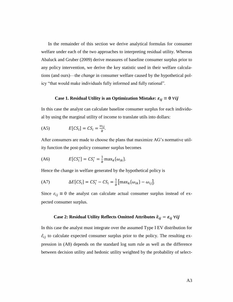
A3

In the remainder of this section we derive analytical formulas for consumer

welfare under each of the two approaches to interpreting residual utility. Whereas

Abaluck and Gruber (2009) derive measures of baseline consumer surplus prior to

any policy intervention, we derive the key statistic used in their welfare calcula-

tions (and ours)—the change in consumer welfare caused by the hypothetical pol-

icy “that would make individuals fully informed and fully rational”.

Case 1. Residual Utility is an Optimization Mistake: 𝜺𝒊𝒋 ≡ 𝟎 ∀𝒊𝒋

In this case the analyst can calculate baseline consumer surplus for each individu-

al by using the marginal utility of income to translate utils into dollars:

(A5) 𝐸[𝐶𝑆𝑖] = 𝐶𝑆𝑖 =𝜔𝑖𝑗

�̂�.

After consumers are made to choose the plans that maximize AG’s normative util-

ity function the post-policy consumer surplus becomes

(A6) 𝐸[𝐶𝑆𝑖∗] = 𝐶𝑆𝑖

∗ =1

�̂�max𝑘{𝜔𝑖𝑘}.

Hence the change in welfare generated by the hypothetical policy is

(A7) ∆𝐸[𝐶𝑆𝑖] = 𝐶𝑆𝑖∗ − 𝐶𝑆𝑖 =

1

�̂�[max𝑘{𝜔𝑖𝑘} − 𝜔𝑖𝑗].

Since 휀𝑖𝑗 ≡ 0 the analyst can calculate actual consumer surplus instead of ex-

pected consumer surplus.

Case 2: Residual Utility Reflects Omitted Attributes �̂�𝒊𝒋 = 𝜺𝒊𝒋 ∀𝒊𝒋

In this case the analyst must integrate over the assumed Type I EV distribution for

휀�̂�𝑗 to calculate expected consumer surplus prior to the policy. The resulting ex-

pression in (A8) depends on the standard log sum rule as well as the difference

between decision utility and hedonic utility weighted by the probability of select-

A4

ing each PDP (e.g. Small and Rosen 1981, Leggett 2002, Abaluck and Gruber

2009).

(A8) 𝐸[𝐶𝑆𝑖] =1

�̂�[𝑙𝑛 ∑ 𝑒�̂�𝑖𝑘

𝑘 + ∑ (𝜔𝑖𝑗 − �̂�𝑖𝑗)𝑒

�̂�𝑖𝑗

∑ 𝑒�̂�𝑖𝑘𝑘𝑗 ] + �̂�.

In the equation, �̂� represents the constant of integration divided by �̂�. It arises

from the assumed Type I EV distribution for 휀�̂�𝑗 and the fact that the level of utili-

ty is unknown.

The policy intervention eliminates the wedge between decision utility and he-

donic utility, simplifying calculation of post-policy consumer surplus:

(A9) 𝐸[𝐶𝑆𝑖∗] =

1

�̂�[𝑙𝑛 ∑ 𝑒𝜔𝑖𝑘

𝑘 ] + 𝐶, where = �̂� +𝜌

�̂� .

If the policy intervention has a direct effect on utility, defined here by 𝜌, then the

post-policy constant of integration, 𝐶, differs from the pre-policy constant of inte-

gration.49

On the other hand, if we follow AG in assuming that the policy has no

direct effect on utility then 𝜌 = 0 and 𝐶 = �̂�. In this case, the change in expected

consumer surplus is

(A10) ∆𝐸[𝐶𝑆𝑖] = 𝐸[𝐶𝑆𝑖∗] − 𝐸[𝐶𝑆𝑖] =

1

�̂�[𝑙𝑛

∑ 𝑒𝜔𝑖𝑘𝑘

∑ 𝑒�̂�𝑖𝑘𝑘− ∑ (𝜔𝑖𝑗 − �̂�𝑖𝑗)

𝑒�̂�𝑖𝑗

∑ 𝑒�̂�𝑖𝑘𝑘𝑗 ].

Equation (A10) isolates the combined welfare effect of imposing the three

normative restrictions on utility that AG emphasize. In contrast, the 27% welfare

gain that AG report in their conclusion is based on the calculation in (A7) that

embeds their normative restrictions along with the added assumption that residual

utility consists entirely of optimization mistakes. Therefore, comparing empirical

results for (A7) and (A10) will reveal the extent to which AG’s reported 27% po-

49 We assume that any direct effect of the policy on utility is additive and invariant to PDP choice so that 𝐸[𝐶𝑆𝑖

∗] =1

�̂�max𝑘{𝜔𝑖𝑘 + 휀𝑖𝑗} =

1

�̂�[𝑙𝑛 ∑ 𝑒𝜔𝑖𝑘+𝜌

𝑘 ] + �̂� =1

�̂�[𝑙𝑛 ∑ 𝑒𝜌

𝑘 𝑒𝜔𝑖𝑘] + �̂� =1

�̂�[𝑙𝑛(𝑒𝜌 ∑ 𝑒𝜔𝑖𝑘

𝑘 )] + �̂� =1

�̂�[𝑙𝑛(𝑒𝜌)] +

1

�̂�[𝑙𝑛 ∑ 𝑒𝜔𝑖𝑘

𝑘 ] + �̂� =1

�̂�[𝑙𝑛 ∑ 𝑒𝜔𝑖𝑘

𝑘 ] + 𝐶.

A5

tential welfare gain is driven by the particular optimization mistakes they empha-

size relative to their novel interpretation of the Type I EV logit error term.

Leggett, Christopher G. 2002. “Environmental Valuation with Imperfect Information”.

Environmental and Resource Economics. 23: 343-355.

Small, Kenneth A. and Harvey S. Rosen. 1981. “Applied Welfare Economics with Dis-

crete Choice Models.” Econometrica. 49(1): 105-130.

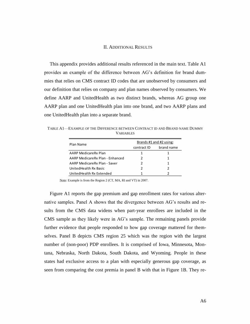
A6

II. ADDITIONAL RESULTS

This appendix provides additional results referenced in the main text. Table A1

provides an example of the difference between AG’s definition for brand dum-

mies that relies on CMS contract ID codes that are unobserved by consumers and

our definition that relies on company and plan names observed by consumers. We

define AARP and UnitedHealth as two distinct brands, whereas AG group one

AARP plan and one UnitedHealth plan into one brand, and two AARP plans and

one UnitedHealth plan into a separate brand.

TABLE A1—EXAMPLE OF THE DIFFERENCE BETWEEN CONTRACT ID AND BRAND NAME DUMMY

VARIABLES

Note: Example is from the Region 2 (CT, MA, RI and VT) in 2007.

Figure A1 reports the gap premium and gap enrollment rates for various alter-

native samples. Panel A shows that the divergence between AG’s results and re-

sults from the CMS data widens when part-year enrollees are included in the

CMS sample as they likely were in AG’s sample. The remaining panels provide

further evidence that people responded to how gap coverage mattered for them-

selves. Panel B depicts CMS region 25 which was the region with the largest

number of (non-poor) PDP enrollees. It is comprised of Iowa, Minnesota, Mon-

tana, Nebraska, North Dakota, South Dakota, and Wyoming. People in these

states had exclusive access to a plan with especially generous gap coverage, as

seen from comparing the cost premia in panel B with that in Figure 1B. They re-

contract ID brand name

AARP MedicareRx Plan 1 1

AARP MedicareRx Plan - Enhanced 2 1

AARP MedicareRx Plan - Saver 2 1

UnitedHealth Rx Basic 2 2

UnitedHealth Rx Extended 1 2

Brands #1 and #2 using:Plan Name

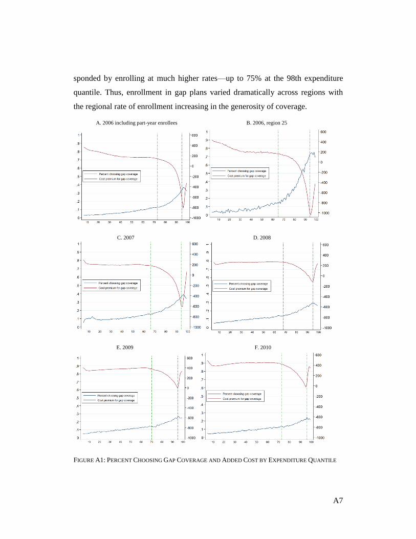
A7

sponded by enrolling at much higher rates—up to 75% at the 98th expenditure

quantile. Thus, enrollment in gap plans varied dramatically across regions with

the regional rate of enrollment increasing in the generosity of coverage.

A. 2006 including part-year enrollees B. 2006, region 25

C. 2007 D. 2008

E. 2009 F. 2010

FIGURE A1: PERCENT CHOOSING GAP COVERAGE AND ADDED COST BY EXPENDITURE QUANTILE

A8

Table A2 summarizes how the average consumer’s chosen plan differs from

other plans the consumer could have chosen. Each cell reports the difference be-

tween an attribute of the consumer’s chosen plan and the mean value of that same

attribute calculated over all of the plans that the consumer could have chosen but

did not. For example, in 2006 the average consumer paid $112 less in out of

pocket costs for prescription drugs under her chosen plan then she would have

paid, on average, if she had enrolled in a different plan than was available to her.

TABLE A2—DIFFERENCE BETWEEN THE CHOSEN PLAN AND THE MEAN ALTERNATIVE

Note: Each row is calculated as the average over all people of the difference between the attribute of their chosen plan and

the average of that same attribute calculated over all others plans in the individual’s choice set. The unit of analysis is the individual person.

Table A3 provides the share of people in 2006 and 2007 that could reduce their

spending by certain amounts by moving from their plan without gap coverage into

the cheapest plan with gap coverage, or by moving from their plan with gap cov-

erage into the cheapest plan without gap coverage.

TABLE A3—POTENTIAL SAVINGS FROM MOVING INTO OR OUT OF A GAP PLAN, 2006-2007

2006 2007 2008 2009 2010

sample size 464,543 566,962 602,992 614,714 629,225

premium (difference in $) -89 -73 -65 -62 -53

out of pocket costs (difference in $) -112 -109 -164 -140 -187

variance of OOP costs (difference in percentage points) -16 27 36 -5 -7

count of top 100 drugs covered (difference in number of drugs) 2 1 1 1 1

CMS quality index (difference in percentage points) 6 5 2 7 0

Percent who could save more than $X

by moving

Into a gap

plan

Out of a

gap plan

Into a gap

plan

Out of a

gap plan

$100 9.9 4.2 6.6 8.6

$300 8.0 2.3 3.7 1.3

$500 4.2 0.1 2.2 0.2

$750 2.5 0.0 1.2 0.1

$1,000 1.4 0.0 0.6 0.0

2006 2007

A9

Table A4 repeats the nonparametric analysis in Table 2 after replacing our

brand dummies (based on company name) with AG’s brand dummies (based on

contract IDs).

TABLE A4— NONPARAMETRIC TEST OF CHOICE INCONSISTENCY WITH BRAND DUMMY VARIABLES

DEFINED USING CONTRACT ID

FIGURE A2—ILLUSTRATION OF THE SUFFICIENT WILLINGNESS TO PAY FOR BRAND

Figure A2 illustrates how we calculate the sufficient willingness to pay

(SWTP) for the bundle of unobserved PDP attributes that vary from brand to

2006 2007 2008 2009 2010

(1) E[cost] year t drug consumption 7 7 10 6 8

(2) E[cost], var(cost) year t drug consumption 25 24 24 26 36

(3) E[cost], var(cost), CMS quality year t drug consumption 35 33 46 42 45

(4) E[cost], var(cost), brand year t drug consumption 74 77 80 87 87

(5) E[cost], var(cost), brand year t or t-1 drug consumption 81 86 91 90

Plan attributes affecting utility Assumption on expected

drug expenditures in year t

% Consumers choosing frontier plans

cost

var

SWTP

b

a

c

A10

brand. To begin, consider a plan, a, that lies on the efficiency frontier in cost-

variance-brand space, where cost means the total cost (premiums plus ex post

OOP drug costs) to the individual. Figure A2 is projected in cost-variance space.

The dots represent other available plans. Plans on the efficiency frontier in cost-

variance space have dark shading; plans off the frontier have light shading. The

area inside the rectangle defined by the dashed lines that intersect at point a de-

fines the portion of the efficiency frontier where other plans dominate a in cost-

variance space. In the figure there are two such plans, b and c. We define SWTP

as the amount of income the consumer gives up by choosing to purchase plan a

instead of the most expensive plan on the portion of the cost-variance frontier that

dominates plan a. Hence, 𝑆𝑊𝑇𝑃 = 𝑐𝑜𝑠𝑡𝑎 − 𝑐𝑜𝑠𝑡𝑏.

SWTP can be interpreted as an arbitrarily close approximation to the willing-

ness to pay for latent attributes of the consumer’s preferred brand for a consumer

with preferences satisfying basic axioms of consumer preference theory. To see

why, suppose that plan a is sold by brand A whereas plans b and c are sold by

brand B, and the two brands differ in a vector of latent quality attributes, q. Con-

sider a consumer who prefers plan b to plan c and is indifferent between plans b

and a such that

𝑈(𝑦 − 𝑐𝑜𝑠𝑡𝑏 , 𝑣𝑎𝑟𝑏 , 𝑞𝐵)

(A11) = 𝑈(𝑦 − 𝑐𝑜𝑠𝑡𝑎, 𝑣𝑎𝑟𝑎 , 𝑞𝐴)

= 𝑈(𝑦 − 𝑐𝑜𝑠𝑡𝑏 − 𝑆𝑊𝑇𝑃, 𝑣𝑎𝑟𝑎, 𝑞𝐴),

where the last line follows from the definition of SWTP. The consumer’s exact

willingness to pay (WTP) to switch from 𝑞𝐵 to 𝑞𝐴, evaluated at the best available

point on the efficiency frontier in cost-variance space, is implicitly defined by the

following equation

(A12) 𝑈(𝑦 − 𝑐𝑜𝑠𝑡𝑏 , 𝑣𝑎𝑟𝑏 , 𝑞𝐵) = 𝑈(𝑦 − 𝑐𝑜𝑠𝑡𝑏 − 𝑊𝑇𝑃, 𝑣𝑎𝑟𝑏 , 𝑞𝐴).

A11

Combining (A11) and (A12) yields the following expression

(A13) 𝑈(𝑦 − 𝑐𝑜𝑠𝑡𝑏 − 𝑆𝑊𝑇𝑃, 𝑣𝑎𝑟𝑎, 𝑞𝐴) = 𝑈(𝑦 − 𝑐𝑜𝑠𝑡𝑏 − 𝑊𝑇𝑃, 𝑣𝑎𝑟𝑏 , 𝑞𝐴).

Assuming the consumer’s preferences satisfy global risk aversion and strong

monotonicity it must be the case that 𝑊𝑇𝑃 > 𝑆𝑊𝑇𝑃. This follows from (A13)

because quality is held constant at 𝑞𝐴. That is, in order to hold utility constant

when the variance decreases from 𝑣𝑎𝑟𝑎 to 𝑣𝑎𝑟𝑏, the risk averse consumer’s in-

come must be reduced. Thus, 𝑊𝑇𝑃 = 𝑆𝑊𝑇𝑃 + 휀, where 휀 is a positive constant

that reflects the willingness to pay to reduce the variance from 𝑣𝑎𝑟𝑎 to 𝑣𝑎𝑟𝑏 at 𝑞𝐴.

Finally, notice that 휀 can be made arbitrarily close to zero (e.g. one tenth of one

cent) without violating completeness, transitivity, strong monotonicity or risk

aversion. It follows that 𝑆𝑊𝑇𝑃 provides an arbitrarily close approximation to the

willingness to pay for latent attributes of the consumer’s preferred brand, condi-

tional on cost and variance, that is sufficient to rationalize the consumer’s ob-

served choice. Also notice that SWTP equals 0 for any plan on the efficiency

frontier in cost-variance space, whereas no value for SWTP can rationalize the

choice of a plan that lies off the efficiency frontier in cost-variance-brand space.

This logic generalizes to any number of plans on the portion of the efficiency

frontier that dominates plan a in cost-variance space. Regardless of the thickness

or sparseness of plans in attribute space, we can always set 휀 to be less than e,

where e is an arbitrarily small positive constant. Likewise, this logic can be gen-

eralized to any assignment of plans to brands by restricting the consumer to have

identical tastes for the vector of latent attributes associated with brands B, C, D,

and so on.

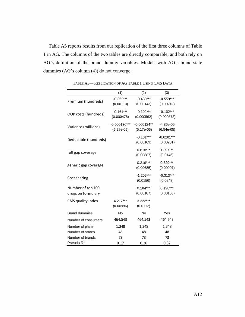
A12

Table A5 reports results from our replication of the first three columns of Table

1 in AG. The columns of the two tables are directly comparable, and both rely on

AG’s definition of the brand dummy variables. Models with AG’s brand-state

dummies (AG’s column (4)) do not converge.

TABLE A5— REPLICATION OF AG TABLE 1 USING CMS DATA

(1) (2) (3)

-0.352*** -0.430*** -0.559***

(0.00110) (0.00143) (0.00249)

-0.161*** -0.102*** -0.102***

(0.000478) (0.000562) (0.000578)

-0.000136*** -0.000124** -4.86e-05

(5.28e-05) (5.17e-05) (6.54e-05)

-0.101*** -0.0201***

(0.00169) (0.00281)

0.818*** 1.897***

(0.00887) (0.0146)

0.216*** 0.529***

(0.00685) (0.00907)

-1.205*** -0.313***

(0.0156) (0.0248)

0.184*** 0.190***

(0.00107) (0.00153)

CMS quality index 4.217*** 3.322***

(0.00996) (0.0112)

Brand dummies No No Yes

Number of consumers 464,543 464,543 464,543

Number of plans 1,348 1,348 1,348

Number of states 48 48 48

Number of brands 73 73 73

Pseudo R2 0.17 0.20 0.32

Cost sharing

Number of top 100

drugs on formulary

Premium (hundreds)

OOP costs (hundreds)

Variance (millions)

Deductible (hundreds)

full gap coverage

generic gap coverage

A13

Table A6 reports results from estimating the model in column (3) of Table 4

for each year from 2006 through 2010.

TABLE A6— SENSITIVITY OF MAIN RESULTS FROM AG’S FULL MODEL TO THE STUDY YEAR

2006 2007 2008 2009 2010

-0.402*** -0.144*** -0.355*** -0.505*** -0.565***

(0.00246) (0.00180) (0.00161) (0.00183) (0.00201)

-0.108*** -0.108*** -0.214*** -0.250*** -0.194***

(0.000573) (0.000580) (0.000836) (0.000849) (0.000734)

-6.48e-05 1.51e-06*** 0.000162*** -0.124*** 1.46e-05

(6.42e-05) (3.39e-07) (4.70e-05) (0.0114) (6.02e-05)

0.0510*** -0.341*** -0.233*** -0.709*** -0.713***

(0.00279) (0.00175) (0.00243) (0.00351) (0.00247)

1.162*** 0.326*** -0.136 1.503*** -1.269***

(0.0146) (0.0225) (8,047) (0.120) (0.0422)

0.356*** -1.065*** -0.184*** 0.281*** 0.328***

(0.00893) (0.00654) (0.00749) (0.00860) (0.00934)

0.683*** 5.198*** 1.067*** -4.636*** -5.149***

(0.0244) (0.0208) (0.0378) (0.0432) (0.0361)

0.175*** 0.275*** 0.181*** 0.150*** 0.334***

(0.00144) (0.00264) (0.00245) (0.00268) (0.00191)

Brand dummies Yes Yes Yes Yes Yes

Number of people 464,543 566,962 602,992 614,714 629,225

Cost sharing

Number of top 100 drugs on

formulary

Premium (hundreds)

OOP costs (hundreds)

Variance (millions)

Deductible (hundreds)

Full gap coverage

Generic gap coverage

A14

Table A7 reports results from estimating the model in column (1) of AG’s Ta-

ble 3 for each year from 2006 through 2010. As shown, the premium coefficient is

slightly below the OOP coefficient for 2008, 2009 and 2010, and the variance co-

efficient has a negative sign for both 2009 and 2010.

TABLE A7— SENSITIVITY OF AG’S BASE RESULTS TO THE STUDY YEAR

Table A8 reports the correlation coefficients between placebo plan characteris-

tics and real plan characteristics calculated across all consumer-plan observations.

TABLE A8— CORRELATIONS BETWEEN PLACEBO AND REAL PLAN CHARACTERISTICS

2006 2007 2008 2009 2010

-0.352*** -0.441*** -0.342*** -0.287*** -0.236***

(0.00110) (0.00111) (0.000832) (0.000793) (0.000719)

-0.161*** -0.176*** -0.382*** -0.297*** -0.296***

(0.000477) (0.000516) (0.000710) (0.000680) (0.000599)

-0.000136*** 4.76e-07* 0.000252*** -1.269*** -0.000307***

(5.28e-05) (2.74e-07) (3.79e-05) (0.0128) (5.09e-05)

4.208*** 5.064*** 1.040*** 1.332*** -0.0115***

(0.00994) (0.00925) (0.00425) (0.00318) (0.00260)

Brand dummies no no no no no

Number of people 464,543 566,962 602,992 614,714 629,225

Premium (hundreds)

OOP costs (hundreds)

Variance (millions)

CMS quality index

premium OOP costs variance deductiblefull gap

coverage

generic gap

coverage

cost

sharing

top 100

count

premium 1.00

OOP costs -0.10 1.00

variance 0.00 0.01 1.00

deductible -0.30 0.13 0.00 1.00

full gap coverage 0.33 -0.05 0.00 -0.13 1.00

generic gap coverage 0.30 -0.08 0.00 -0.30 -0.06 1.00

cost sharing -0.33 0.18 0.00 -0.04 0.04 -0.08 1.00

top 100 count 0.21 -0.10 0.00 -0.09 0.08 0.09 -0.43 1.00

count 8 -0.01 -0.02 0.00 -0.08 -0.03 -0.02 -0.06 0.05

count 9 0.06 -0.03 0.00 -0.07 0.08 0.06 -0.03 0.07

count D 0.06 0.00 0.00 -0.03 0.09 -0.01 0.01 -0.05

count d -0.01 0.00 0.00 0.04 -0.05 0.11 -0.05 0.06

count e 0.01 0.03 0.00 0.08 -0.06 0.07 0.02 0.02

count k 0.07 -0.02 0.00 -0.07 -0.11 0.14 -0.13 0.07

count l -0.06 0.01 0.00 0.04 -0.01 -0.03 0.06 -0.03

count o 0.03 0.00 0.00 0.01 -0.03 0.11 0.01 0.04

count r 0.06 -0.01 0.00 -0.03 0.05 -0.01 0.02 -0.03

count x -0.15 0.04 0.00 0.10 0.07 -0.29 0.15 -0.14

A15

TABLE A9— RESULTS FROM MODELS WITH PLACEBO PLAN CHARACTERISTICS

Variable Coefficient

-0.0243***

(0.00568)

-0.0523***

(0.00604)

-0.0154**

(0.00653)

0.158***

(0.00701)

0.0929***

(0.00737)

-0.215***

(0.00450)

0.0301***

(0.00631)

-0.0522***

(0.00782)

-0.228***

(0.00716)

-0.429***

(0.00260)

-0.108***

(0.000571)

-5.11e-05

(6.38e-05)

-0.0250***

(0.00315)

1.314***

(0.0151)

0.383***

(0.00913)

1.019***

(0.0254)

0.172***

(0.00141)

Brand dummies Yes

Number of people 464,543

Cost sharing

Number of top 100 drugs on

formulary

Premium (hundreds)

OOP costs (hundreds)

Variance (millions)

Deductible (hundreds)

Full gap coverage

Generic gap coverage

Count of k's

Count of l's

Count of o's

Count of r's

Count of 8's

Count of 9's

Count of D's

Count of d's

Count of e's

A16

Table A10 shows results provided to us by AG regarding the placebo test. It al-

so compares the implied WTP for actual plan financial attributes from AG’s 2011

article, our replication of them, their new results and our replication of them. The

results on the financial attributes show that their new results diverge from their

old ones by at least $90 for 4 of the 5 attributes. In contrast, all of ours are within

$65. The lower half of the Table reports the results from their placebo attributes

and our replication of their placebo model. For several reasons these results are

not directly comparable to the results we report, yet they yield similar qualitative

insights: first, they replaced our count variables for each alphanumeric with indi-

cator variables for any positive count of the alphanumeric. Although this makes it

impossible to isolate the marginal effects comparable to the financial attributes, to

facilitate comparison we replicate their approach here. Second, they stated that

they normalized these placebo attributes to zero, relative to whether a “9” is pre-

sent, but they did not implement any similar normalization for the financial attrib-

utes. Third, two separate values are reported for the presence of “k”, and no val-

ues are reported for the presence of an “e”. Nonetheless, as with our results the

test implies that these imaginary attributes influence people’s PDP choices in

economically meaningful ways. For example, AG’s results imply that people

would be willing to pay $117 more for a plan with a “d”, “o” and “l” in the en-

crypted plan ID than for a plan with three “9s”, whereas they would pay $124 for

a plan with three “9s” to avoid a plan with an “8”, “D” and “x”. Both of these, as

well as a number of other combinations, exceed the magnitude estimated for of all

of the real plan attributes in AG 2011 other than full gap coverage.

A17

TABLE A10— COMPARING ESTIMATED WILLINGNESS TO PAY FOR REAL AND PLACEBO PLAN CHARACTERISTICS FROM AG 2011 BASELINE

MODEL OUR REPLICATION OF AG, AND NEW RESULTS PROVIDED BY AG

AG 2011

WTP ($) WTP ($)

Difference

from AG

2011 ($) WTP ($)

Difference

from AG

2011 WTP ($)

Difference

from AG

2011

Decreasing the deductible from $250 to $0 80 15 -65 293 213 20 -60

Covering one additional "top 100" drug 50 40 -10 9 -41 39 -11

Adding generic gap coverage 50 89 39 142 92 87 37

Increasing cost sharing from 25% to 65% 80 95 15 541 461 92 12

Adding full gap coverage 300 306 6 434 134 297 -3

Encrypted plan ID includes at least one

“d” 60 -97

“o” 40 -32

“k”--result 1 29 11

“k”--result 2 -27 --

“l” 17 -40

“r” 16 14

"9" Reference -30

"e" Not provided -60

“8” -7 -37

“D” -34 -38

“x” -83 -77

Our replication

AG placebo

specification Our replication

A18

TABLE A11— RESULTS FROM FIVE LARGEST REGIONS DEFINING BRAND DUMMIES BASED ON

CONTRACT ID

region

25

region

17

region

11

region

22

region

4

Estimated parameter ratios

1.3 7.3 9.7 5.7 78.9

(0.0) (0.2) (0.3) (0.2) (5.4)

0.0 0.0 0.0 -0.3 0.0

(0.0) (0.0) (0.0) (0.1) (0.0)

-3.0 0.5 0.3 -0.2 0.0

(0.1) (0.0) (0.0) (0.0) (0.0)

-2.9 -3.3 -4.3 -3.2 -4.4

(0.1) (0.1) (0.0) (0.1) (0.0)

0.6 1.8 -0.9 -2.3 -1.8

(0.5) (0.1) (0.0) (0.1) (0.0)

-2.9 2.4 -2.8 5.0 1.8

(0.8) (0.1) (0.2) (0.2) (0.1)

-0.3 -0.3 -0.2 -0.3 -0.1

(0.0) (0.0) (0.0) (0.0) (0.0)

Welfare loss (% of costs)

ε ≡ 0 101 19 25 25 19

ε is unrestricted 19 9 17 8 20

PDP Menu

# plans 41 42 43 47 44

# brands 17 17 19 21 19

# plans w/ gap coverage 7 6 8 6 6

# plans w/ no deductible 23 25 25 27 25

Consumers

mean age 76 78 76 76 78

% with dementia 6.2 8.2 7.8 8.6 9.4

% off cost-var frontier 74 79 76 72 82

% off cost-var-brand frontier 36 27 26 25 16

mean potential savings 621 469 543 517 606

number 46,997 37,939 30,138 29,387 24,162

premium / OOP

variance / premium

deductible / premium

top 100 / premium

full gap / premium

generic gap / premium

cost share / premium

A19

Table A12 replicates the results in Table 5 after limiting the sample to white

females under 80 who have not been diagnosed with Alzheimer’s, dementia, or

depression. See the discussion of Table 5 for additional details.

TABLE A12: RESULTS FROM MODELS IN TABLE 5 BUT WITH THE SAMPLE RESTRICTED TO WHITE

FEMALES AGE<80 WITHOUT ALZHEIMER’S DISEASE OR DEMENTIA OR DEPRESSION

United

States

region

25

region

17

region

11

region

22

region

4

Decision utility parameters

3.3 1.0 5.6 4.2 1.7 -5.0

(0.0) (0.1) (0.2) (0.3) (0.2) (2.1)

0.0 0.0 0.0 -0.1 -0.2 -0.8

(0.0) (0.0) (0.0) (0.0) (0.2) (0.6)

-0.1 -3.6 0.1 0.3 -0.7 4.9

(0.0) (0.3) (0.0) (0.1) (0.2) (1.8)

-2.5 -2.6 -3.0 -3.3 1.6 -8.3

(0.0) (0.2) (0.1) (0.2) (0.9) (1.6)

-0.8 2.0 1.9 -0.1 -3.6 3.2

(0.0) (1.0) (0.2) (0.1) (0.6) (2.0)

-2.8 -4.2 2.7 -9.1 5.7 -30.5

(0.1) (1.7) (0.3) (0.6) (1.2) (11.9)

-0.4 -0.3 -0.3 -0.4 -0.6 -0.1

(0.0) (0.0) (0.0) (0.0) (0.1) (0.1)

Welfare loss (% of costs)

ε ≡ 0 41 94 18 31 63 --

ε is unrestricted 7 27 8 11 4 --

Number of consumers 155,115 17,196 11,448 9,869 9,174 6,916

top 100 / premium

full gap / premium

generic gap / premium

cost share / premium

premium / OOP

variance / premium

deductible / premium

A20

Table A13 reports summary statistics of the distribution of region-level results,

restricted to the 24 regions with statistically significant positive estimates for the

marginal utility of income. The last row reports the premium-to-OOP ratio that is

predicted from an extended version of AG’s DU model from equation (4) that al-

lows the premium-to-OOP ratio to vary with the number of plans in the choice

set, the number of brands, the number of plans with gap coverage, the number of

plans with zero deductible, the consumer’s age, and an indicator for whether the

consumer is diagnosed with dementia including Alzheimer’s disease. Coefficient

estimates are reported in Table A16.

TABLE A13—SUMMARY STATISTICS OF THE DISTRIBUTION OF REGION-SPECIFIC ESTIMATED PA-

RAMETER RATIOS, PDP MENU ATTRIBUTES, CONSUMER ATTRIBUTES AND NONPARAMETRIC OUT-

COMES, 2006

Mean

Standard

deviation Minimum

25th

Percentile Median

75th

Percentile Maximum

Estimated parameter ratios

premium / OOP 4.8 2.8 1.1 2.7 4.2 6.6 12.3

variance / premium -0.2 0.3 -0.8 -0.4 -0.2 0.0 0.6

deductible / premium -0.4 1.8 -7.5 -0.1 0.1 0.2 1.1

full gap / premium -3.0 1.7 -4.4 -4.2 -3.3 -2.5 0.6

generic gap / premium -1.6 2.7 -9.5 -1.7 -1.1 -0.4 1.6

cost share / premium -4.5 13.0 -25.8 -10.7 -6.0 -2.0 48.1

top 100 / premium -0.4 0.2 -0.9 -0.6 -0.4 -0.3 -0.2

Welfare loss (% of costs)

ε ≡ 0 42.1 24.1 17.7 25.1 33.6 54.5 109.9

ε is unrestricted 14.9 13.1 3.3 8.8 11.3 15.9 68.4

PDP Menu

# plans 42 9 38 41 42 44 47

# brands 19 4 17 18 19 20 23

# plans w/ gap coverage 7 1 6 6 7 7 9

Consumers

number 16,638 11,036 3,710 7,035 14,712 23,659 46,997

mean age 76 15 75 75 76 76 78

% with Alzheimer's 7 2 6 7 8 8 9

% off cost-var frontier 75 15 67 72 75 78 82

% off cost-var-brand frontier 19 6 8 16 19 23 34

mean potential savings 506 103 355 485 508 535 621

premium / oop ratio predicted

by interaction model

4.1 0.6 3.3 3.8 4.0 4.2 5.9

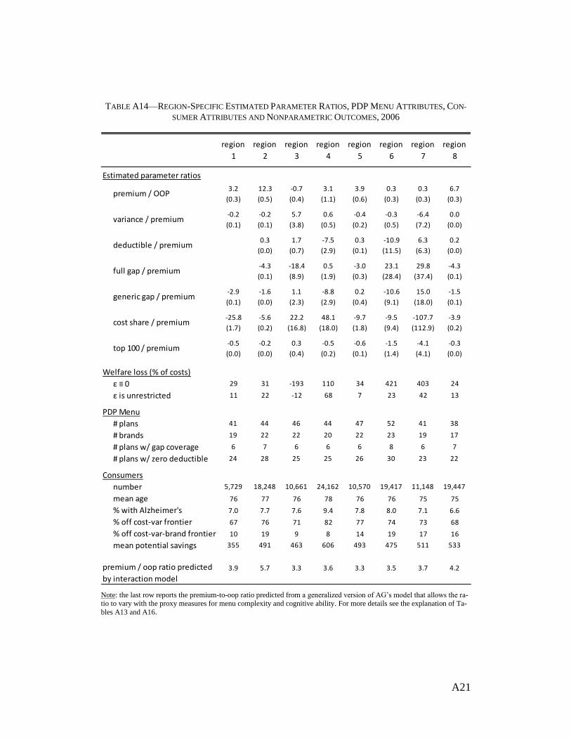
A21

TABLE A14—REGION-SPECIFIC ESTIMATED PARAMETER RATIOS, PDP MENU ATTRIBUTES, CON-

SUMER ATTRIBUTES AND NONPARAMETRIC OUTCOMES, 2006

Note: the last row reports the premium-to-oop ratio predicted from a generalized version of AG’s model that allows the ra-tio to vary with the proxy measures for menu complexity and cognitive ability. For more details see the explanation of Ta-

bles A13 and A16.

region

1

region

2

region

3

region

4

region

5

region

6

region

7

region

8

Estimated parameter ratios

3.2 12.3 -0.7 3.1 3.9 0.3 0.3 6.7

(0.3) (0.5) (0.4) (1.1) (0.6) (0.3) (0.3) (0.3)

-0.2 -0.2 5.7 0.6 -0.4 -0.3 -6.4 0.0

(0.1) (0.1) (3.8) (0.5) (0.2) (0.5) (7.2) (0.0)

0.3 1.7 -7.5 0.3 -10.9 6.3 0.2

(0.0) (0.7) (2.9) (0.1) (11.5) (6.3) (0.0)

-4.3 -18.4 0.5 -3.0 23.1 29.8 -4.3

(0.1) (8.9) (1.9) (0.3) (28.4) (37.4) (0.1)

-2.9 -1.6 1.1 -8.8 0.2 -10.6 15.0 -1.5

(0.1) (0.0) (2.3) (2.9) (0.4) (9.1) (18.0) (0.1)

-25.8 -5.6 22.2 48.1 -9.7 -9.5 -107.7 -3.9

(1.7) (0.2) (16.8) (18.0) (1.8) (9.4) (112.9) (0.2)

-0.5 -0.2 0.3 -0.5 -0.6 -1.5 -4.1 -0.3

(0.0) (0.0) (0.4) (0.2) (0.1) (1.4) (4.1) (0.0)

Welfare loss (% of costs)

ε ≡ 0 29 31 -193 110 34 421 403 24

ε is unrestricted 11 22 -12 68 7 23 42 13

PDP Menu

# plans 41 44 46 44 47 52 41 38

# brands 19 22 22 20 22 23 19 17

# plans w/ gap coverage 6 7 6 6 6 8 6 7

# plans w/ zero deductible 24 28 25 25 26 30 23 22

Consumers

number 5,729 18,248 10,661 24,162 10,570 19,417 11,148 19,447

mean age 76 77 76 78 76 76 75 75

% with Alzheimer's 7.0 7.7 7.6 9.4 7.8 8.0 7.1 6.6

% off cost-var frontier 67 76 71 82 77 74 73 68

% off cost-var-brand frontier 10 19 9 8 14 19 17 16

mean potential savings 355 491 463 606 493 475 511 533

premium / oop ratio predicted

by interaction model

3.9 5.7 3.3 3.6 3.3 3.5 3.7 4.2

cost share / premium

top 100 / premium

premium / OOP

variance / premium

deductible / premium

full gap / premium

generic gap / premium

A22

TABLE A14 (CONTINUED)—REGION-SPECIFIC ESTIMATED PARAMETER RATIOS, PDP MENU AT-

TRIBUTES, CONSUMER ATTRIBUTES AND NONPARAMETRIC OUTCOMES, 2006

Note: the last row reports the premium-to-oop ratio predicted from a generalized version of AG’s model that allows the ra-tio to vary with the proxy measures for menu complexity and cognitive ability. For more details see the explanation of Ta-

bles A13 and A16.

region

9

region

10

region

11

region

12

region

13

region

14

region

15

region

16

Estimated parameter ratios

0.3 7.8 3.3 6.2 5.5 2.1 3.6 2.6

(0.3) (0.4) (0.2) (0.3) (0.4) (0.2) (0.2) (0.2)

-11.1 -0.2 0.0 -0.4 -0.2 -0.4 -0.7 0.0

(12.0) (0.1) (0.0) (0.1) (0.1) (0.2) (0.1) (0.2)

-17.3 -0.1 0.1 -0.1 0.6 0.2 -0.1 0.0

(18.9) (0.0) (0.0) (0.0) (0.0) (0.1) (0.0) (0.1)

13.5 -4.4 -3.3 -4.4 -4.2 -1.2 -4.2 -2.5

(20.1) (0.1) (0.1) (0.1) (0.1) (0.5) (0.1) (0.3)

21.8 -1.1 -0.1 -1.4 -1.0 0.5 -1.2 -0.6

(25.5) (0.1) (0.1) (0.1) (0.2) (0.3) (0.1) (0.1)

40.0 -2.0 -10.9 -3.5 -12.7 -14.7 -11.0 -7.6

(44.9) (0.2) (0.6) (0.2) (0.6) (1.5) (0.6) (0.6)

-1.4 -0.2 -0.5 -0.4 -0.4 -0.9 -0.5 -0.4

(1.3) (0.0) (0.0) (0.0) (0.0) (0.1) (0.0) (0.0)

Welfare loss (% of costs)

ε ≡ 0 398 24 38 27 34 66 40 42

ε is unrestricted 61 12 9 16 21 9 11 7

PDP Menu

# plans 45 42 43 41 40 43 42 45

# brands 21 19 20 19 19 20 19 19

# plans w/ gap coverage 6 7 8 6 6 7 7 9

# plans w/ zero deductible 24 24 25 23 23 25 25 29

Consumers

number 7,650 17,268 30,138 16,928 10,389 15,932 23,832 9,340

mean age 76 75 76 75 76 76 76 75

% with Alzheimer's 7.4 8.0 7.8 7.9 7.5 7.7 7.0 6.1

% off cost-var frontier 79 79 76 71 74 72 76 78

% off cost-var-brand frontier 20 20 15 23 22 16 24 21

mean potential savings 558 495 543 522 499 495 540 427

premium / oop ratio predicted

by interaction model

3.3 3.9 4.0 3.7 3.9 3.9 4.0 4.6

cost share / premium

top 100 / premium

premium / OOP

variance / premium

deductible / premium

full gap / premium

generic gap / premium

A23

TABLE A14 (CONTINUED)—REGION-SPECIFIC ESTIMATED PARAMETER RATIOS, PDP MENU AT-

TRIBUTES, CONSUMER ATTRIBUTES AND NONPARAMETRIC OUTCOMES, 2006

Note: the last row reports the premium-to-oop ratio predicted from a generalized version of AG’s model that allows the ra-tio to vary with the proxy measures for menu complexity and cognitive ability. For more details see the explanation of Ta-

bles A13 and A16.

region

17

region

18

region

19

region

20

region

21

region

22

region

23

region

24

Estimated parameter ratios

7.0 4.4 -0.2 4.7 2.2 1.9 8.1 9.9

(0.2) (0.3) (0.3) (0.4) (0.6) (0.1) (0.6) (0.6)

0.0 -0.6 0.0 -0.3 0.0 -0.8 -0.2 -0.4

(0.0) (0.1) (0.0) (0.1) (0.3) (0.2) (0.1) (0.1)

0.0 0.2 15.0 0.0 -1.6 -0.5 0.2 0.1

(0.0) (0.0) (25.6) (0.1) (0.7) (0.1) (0.0) (0.0)

-3.5 -3.4 -46.6 -3.5 -3.3 0.6 -3.7 -4.0

(0.1) (0.1) (74.3) (0.2) (0.7) (0.5) (0.1) (0.1)

1.6 -1.1 -1.8 -9.5 -2.8 -0.3 -0.8

(0.1) (0.1) (0.2) (2.9) (0.3) (0.1) (0.1)

3.8 -6.8 32.5 -1.3 3.2 5.0 -2.5 -2.2

(0.2) (0.4) (58.0) (0.5) (2.4) (0.6) (0.3) (0.2)

-0.4 -0.4 3.5 -0.3 -0.6 -0.7 -0.4 -0.2

(0.0) (0.0) (6.4) (0.0) (0.1) (0.0) (0.0) (0.0)

Welfare loss (% of costs)

ε ≡ 0 18 31 -295 24 40 62 20 23

ε is unrestricted 9 11 -50 10 8 3 10 16

PDP Menu

# plans 42 41 40 38 39 47 42 40

# brands 18 18 17 17 18 22 18 17

# plans w/ gap coverage 6 6 6 6 6 6 7 7

# plans w/ zero deductible 25 25 24 23 24 27 25 25

Consumers

number 37,939 13,492 7,317 6,785 4,265 29,387 6,880 7,499

mean age 78 76 75 75 75 76 76 77

% with Alzheimer's 8.2 7.9 8.5 6.9 7.8 8.6 7.6 7.5

% off cost-var frontier 79 73 79 74 75 72 79 78

% off cost-var-brand frontier 15 21 30 26 19 18 24 24

mean potential savings 469 491 591 520 547 517 520 536

premium / oop ratio predicted

by interaction model

4.0 4.1 4.1 4.3 4.2 3.5 4.1 4.5

cost share / premium

top 100 / premium

premium / OOP

variance / premium

deductible / premium

full gap / premium

generic gap / premium

A24

TABLE A14 (CONTINUED)—REGION-SPECIFIC ESTIMATED PARAMETER RATIOS, PDP MENU AT-

TRIBUTES, CONSUMER ATTRIBUTES AND NONPARAMETRIC OUTCOMES, 2006

Note: the last row reports the premium-to-oop ratio predicted from a generalized version of AG’s model that allows the ra-tio to vary with the proxy measures for menu complexity and cognitive ability. For more details see the explanation of Ta-

bles A13 and A16.

region

25

region

26

region

27

region

28

region

29

region

30

region

31

region

32

Estimated parameter ratios

1.1 -0.2 4.5 1.5 1.8 3.9 -2.2 5.6

(0.0) (0.9) (0.6) (0.7) (2.0) (0.4) (0.7) (0.4)

0.0 0.9 -0.8 0.1 -3.1 0.0 2.7 0.0

(0.0) (7.1) (0.2) (0.3) (3.6) (0.0) (1.0) (0.0)

-3.6 6.5 0.2 -0.7 0.8 1.1 1.5 0.5

(0.2) (22.6) (0.1) (0.6) (0.5) (0.1) (0.4) (0.0)

-2.9 -45.5 -3.1 -0.3 1.8 -2.3 -9.1 -3.1

(0.1) (147.7) (0.3) (2.3) (7.3) (0.3) (1.5) (0.1)

0.8 -0.7 -2.9 0.3 -0.8 -1.1

(0.6) (0.2) (1.3) (1.4) (0.3) (0.1)

-3.2 -29.3 -6.4 -10.1 -25.8 -22.1 0.3 -6.4

(0.9) (114.5) (0.8) (5.0) (25.8) (1.9) (2.1) (0.4)

-0.4 62.6 -0.3 -0.7 -0.7 -0.6 0.3 -0.4

(0.0) (225.2) (0.0) (0.3) (0.7) (0.0) (0.2) (0.0)

Welfare loss (% of costs)

ε ≡ 0 92 -324 33 79 109 59 -86 31

ε is unrestricted 24 -118 10 4 9 32 -29 15

PDP Menu

# plans 41 43 43 43 44 45 44 47

# brands 23 19 19 20 20 22 20 20

# plans w/ gap coverage 7 6 7 6 7 6 6 7

# plans w/ zero deductible 23 26 26 25 25 25 23 28

Consumers

number 46,997 1,587 3,710 4,926 1,703 12,314 5,594 23,141

mean age 76 75 76 75 75 76 76 76

% with Alzheimer's 6.2 6.9 7.4 5.7 6.4 6.6 6.3 6.6

% off cost-var frontier 74 74 73 69 78 74 76 78

% off cost-var-brand frontier 34 13 18 13 17 18 20 17

mean potential savings 621 414 468 444 510 483 532 521

premium / oop ratio predicted

by interaction model

5.9 3.9 4.1 3.7 3.7 3.4 3.4 3.8

premium / OOP

variance / premium

deductible / premium

full gap / premium

generic gap / premium

cost share / premium

top 100 / premium

A25

FIGURE A3—RATIO OF PREMIUM-TO-OOP COEFFICIENTS IN 2006, BY CMS REGION USING AG’S

DEFINITION OF BRAND DUMMIES BASED ON CONTRACT ID

Note: The figure reports the premium-to-OOP coefficient ratio obtained by estimating region-specific models with contract

id dummies. The econometric specification is the same as the national model in column 2 of Table 4. In regions with light-

shaded numbers, we fail to reject the null hypothesis that the marginal utility of income is negative at the 5% level. All es-timates are statistically indistinguishable from 1 at the 5% level.

A26

Table A15 provides the coefficients and standard errors from meta-regressions

of the conditional relationship between the premium-to-OOP ratio and proxy

measures for menu complexity and cognitive ability. The models are limited to

the 24 regions with statistically significant positive estimates for the marginal util-

ity of income. The main text provides additional details.

TABLE A15: RESULTS FROM MODELS OF THE REGION-LEVEL ESTIMATES FOR AG’S PARAMETRIC

MEASURES OF CHOICE QUALITY ON PROXY MEASURES FOR MENU COMPLEXITY AND COGNITIVE

ABILITY

Note: *** p<0.01, ** p<0.05, * p<0.1

(1) (2) (3) (4) (5)

ε ≡ 0 ε ≠ 0

-0.508 -0.559 1.100 0.707

(0.553) (0.577) (4.420) (2.386)

-0.234 -0.214 7.613* 1.082

(0.521) (0.553) (4.241) (2.289)

-0.284 0.0865 0.837 0.703

(0.896) (0.943) (7.227) (3.901)

0.858 0.802 -4.213 -2.574

(0.710) (0.725) (5.555) (2.998)

0.706 0.811 8.567 10.43**

(0.960) (1.004) (7.697) (4.154)

0.277 0.445 -3.410 0.129

(0.861) (0.947) (7.261) (3.919)

11.33 -50.83 -52.80 -678.1 -769.2**

(10.30) (69.39) (71.95) (551.5) (297.7)

Observations 24 24 24 24 24

R2 0.151 0.061 0.239 0.404 0.422

Adjusted R2 -0.028 -0.028 -0.029 0.193 0.218

P-value of model Wald Chi-Square 0.514 0.515 0.523 0.136 0.111

premium-to-OOP coef ratio

% welfare loss

Constant

Number of plans

Number of brands

% with Alzheimer's

Number of plans w/ gap coverage

Number of plans w/ zero deductible

mean age

A27

To check robustness of the results from the meta-regression in equation (9) we

estimate AG’s DU model (4) after adding interactions between the OOP ratio and

the proxy measures for menu complexity and cognitive ability. This logit model

accounts for variation in menu complexity across CMS regions and for variation

in cognitive ability within and across CMS regions. Each of the interaction coeffi-

cients is statistically significant at the 1% level. To evaluate their economic mag-

nitudes we use the estimates to predict how the premium-to-oop ratio would

change as we move from the lowest value of each variable observed in our data to

the highest value, while evaluating all other variables at their means. The resulting

ranges are reported in the last two columns of Table A16. For example, the results

in the first row of the table imply that increasing the number of plans in a con-

sumer’s choice set from 38 plans to 52 plans would decrease the premium-to-oop

ratio from 4.6 to 2.9, contrary to the hypothesis of choice overload.

TABLE A16: ESTIMATED EFFECTS OF PROXY MEASURES FOR MENU COMPLEXITY AND COGNITIVE

ABILITY ON THE PREMIUM-TO-OOP RATIO

Note: The estimated coefficients on premium and OOP are -0.406 and -0.066 respectively. Both have p-values of zero out

to four decimal places.

Table A17 provides results from validation tests for the cases where the set of

brands in an estimation region spans the set of brands in the prediction region.

Two pairs of regions meet this criterion in 2006. As a result, we estimate the

AG’s two competing models for region 14 and then use the resulting coefficients

mean min maxinteraction

with OOP

standard

error

predicted

at the Min

predicted

at the Max

Number of plans in choice set 43.15 38 52 -0.0035 (0.0004) 4.6 2.9

Number of brands in choice set 20.05 17 23 -0.0014 (0.0003) 4.0 3.7

Number of plans with gap coverage 6.67 6 9 0.0033 (0.0007) 3.7 4.1

Number of plans with zero deductible 25.08 22 30 0.0043 (0.0005) 3.4 4.7

Age 76.04 66 108 0.0002 (0.0001) 3.7 4.0

Dementia including Alzeheimer's 0.08 0 1 -0.0102 (0.0014) 3.8 3.5

Premium-to-OOP ratioSummary statistics Econometric estimates

A28

to predict outcomes in region 15, and we use estimates for region 30 to predict

outcomes in region 28. Both region pairs are similar in their consumer popula-

tions and PDP menu complexity. AG’s EUM model yields closer out-of-sample

predictions than their DU model in every case but one. The shading indicates

which prediction is closer to the data.

TABLE A17: RESULTS FROM BETWEEN-REGION VALIDATION TESTS FOR THE ONLY TWO PAIRS OF

REGIONS IN 2006 FOR WHICH ONE REGION’S BRANDS ARE NESTED WITHIN THE OTHER’S

data AG's DU AG's EUM data AG's DU AG's EUM

Percent of consumers choosing:

gap coverage 11 11 13 6 6 9

dominated plan 16 18 17 18 19 17

min cost plan within brand 47 40 41 41 35 40

Median consumer expenditures ($)

premium + OOP 1,261 1,262 1,267 1,074 1,093 1,095

overspending on dominated plans 0 65 58 0 63 58

Market concentration

Hirfindahl-Hirschman index 25 25 25 25 25 25

market share of top brand 44 44 44 39 39 39

Percent of consumers choosing:

gap coverage 9 6 10 18 11 13

dominated plan 12 25 19 24 18 17

min cost plan within brand 50 32 40 42 40 41

Median consumer expenditures ($)

premium + OOP 1,096 1,205 1,178 1,418 1,352 1,355

overspending on dominated plans 0 102 70 0 67 57

Market concentration

Hirfindahl-Hirschman index 44 30 31 0 21 27 26

market share of top brand 62 42 46 0 31 45 44

region 15 region 28

Out-of-sample data and predictions

region 14 → 15 region 30 → 28

In-sample data and predictions

region 14 region 30

A29

Table A18 provides results from the national validation test shown in Table 6

except using the root mean square error in predictions across regions in place of

the mean absolute error.

TABLE A18— NONRANDOM HOLDOUT SAMPLE TESTS OF MODEL VALIDATION, 2006

Note: RMSE refers to the root mean square error between the regional-level model predictions and data, weighted across regions by the number of people in the sample in the region. The results are based on every possible pairwise combination

of regions in 2006 except that they exclude regions 33 and 34 (HI and AK), and the lower half also excludes region 26

(NM). Thus the values in the top half are based on the results from all 992 of the possible regional out-of-sample predic-tions while those in the lower half are based on 930 of them.

AG's DU AG's EUM AG's DU AG's EUM

data

Percent of consumers choosing:

gap coverage 13 0 7 9 7

dominated plan 20 5 6 8 7

min cost plan within brand 52 8 9 11 9

Median consumer expenditures ($)

premium + OOP 1,255 16 46 113 88

overspending on dominated plans 0 72 55 70 51

Market concentration

Hirfindahl-Hirschman index 25 11 15 11 15

market share of top brand 37 12 18 14 18

Percent of consumers choosing:

gap coverage 13 0 4 9 8

dominated plan 20 2 4 9 9

min cost plan within brand 52 6 9 14 13

Median consumer expenditures ($)

premium + OOP 1,256 16 21 102 101

overspending on dominated plans 0 82 71 88 70

Market concentration

Hirfindahl-Hirschman index 25 0 0 14 13

market share of top brand 37 0 0 18 17

Using Brand Indicators for Quality

In-sample fit Out-of-sample fit

RMSE RMSE

Using CMS Star Ratings for Quality

A30

Table A19 provides results from the national validation test suggested to us by

Abaluck and Gruber. Specifically, we estimate the models using the 2006 data

from 31 regions and use it to predict a single out-of-sample region, repeated using

each of the 32 regions as the holdout region (excluding Alaska and Hawaii). This

is very similar to an in-sample validation test as the set of plans and plan attrib-

utes in the single out-of-sample region is typically very close to being nested

within the in-sample set (see Keane and Wolpin 2007). As before the measures of

market concentration are defined at the region level as that is the policy-relevant

market definition. Hence while the models with brand indicators match the market

concentration perfectly across the 31 in-sample regions in each of the 32 separate

tests (yielding a mean absolute deviation of 0), they do not perfectly predict the

region-level market concentration for any single given in-region sample.

A31

TABLE A19— RESULTS FROM THE NATIONAL MODEL VALIDATION TESTS SUGGESTED BY

ABALUCK AND GRUBER

Note: | Model error | refers to the mean absolute deviation between the model predictions and data.

AG's DU AG's EUM AG's DU AG's EUM

data

Percent of consumers choosing:

gap coverage 13 0 2 6 6

dominated plan 20 2 2 6 6

min cost plan within brand 52 3 4 6 5

Median consumer expenditures ($)

premium + OOP 1,255 4 15 61 60

overspending on dominated plans 0 63 51 63 51

Market concentration

Hirfindahl-Hirschman index 25 11 14 11 14

market share of top brand 37 9 17 11 17

Percent of consumers choosing:

gap coverage 13 0 2 6 6

dominated plan 20 1 1 5 5

min cost plan within brand 52 7 8 8 9

Median consumer expenditures ($)

premium + OOP 1,255 10 14 61 57

overspending on dominated plans 0 64 61 71 63

Market concentration

Hirfindahl-Hirschman index 25 4 4 5 4

market share of top brand 37 6 6 8 7

Using Brand Indicators for Quality

In-sample fit Out-of-sample fit

|model error | |model error |

Using CMS Star Ratings for Quality