china s international trade and air pollution in the u.s.€¦ · china’s international trade and...

China’s international trade and air pollution in the U.S.

Lin et al.

Supporting Information:

Materials and Methods

Methods Summary

1. Input-Output Model

2. Data Sources

3. Monte Carlo method for uncertainty evaluation

4. Total emissions in China

5. Emission Intensity and trade-induced emissions

6. GEOS-Chem simulations to analyze impacts of international trade on global

atmospheric environment

7. Understanding the high emission/GDP ratio of China relative to the U.S. level

and impacts of less advanced technology level

Tables S1-S11

Figures S1-S8

References

Materials and Methods

Methods Summary

Calculation of emissions embodied in exports and imports is based on an

input-output analysis of the monetary outputs of the economic processes required to

produce a particular good or service, multiplied by sector-specific emission

intensities. Emissions from ocean shipping vessels are not included in the analysis.

Sectoral emission intensities are calculated as total Chinese emissions (which are

estimated by a technology-based, bottom-up approach) divided by total monetary

outputs from the respective sectors. We use a Monte Carlo method to quantify

uncertainty associated with errors in emission factors, economic statistics and the

input-output analysis itself. Emissions of carbon dioxide (CO2) are calculated with a

similar approach, and the resulting emissions embodied in trade are consistent with

previous studies. The global chemical transport model GEOS-Chem (version

8-03-02; on the 2.5º long x 2º lat grid) is used to simulate the impacts of trade-related

pollution on global atmospheric environment.

1. Input-Output Model

Our study is based on an input-output analysis (IOA) that captures indirect

environmental impacts caused by upstream production and is thus suitable for

estimating embodied emissions (1-3). The method is used commonly for analyzing

trade-induced emissions of carbon dioxide (CO2) (4-8).

Figure S1 shows the general methodology for this study. For a given economic

sector, emissions embodied in exports/imports are calculated as trade-related

monetary outputs multiplied by emission intensity deduced as total emissions of

China divided by total monetary outputs. Total emissions are estimated with a

technology-based bottom-up approach (9, 10) and total outputs and trade-related

outputs are derived based on the IOA. To remove to impact of inflation on the

monetary outputs, the producer price index (PPI) (11) is used to adjust all monetary

data based on prices in 2005 for a consistent analysis over 2000-2009.

1.1 A general structure for calculating emissions embodied in international trade

Emissions embodied in exports (EEE) result from production and transportation

of goods for exports. As shown in Eq. 1, they are calculated as the sum over all

related sectors of exports ( eX ; in monetary units) multiplied by emission intensity

( F ). Correspondingly, total emissions in China (P; including EEE and those related

to domestic consumption) are calculated as the sum over all sectors of emission

intensity multiplied by total monetary outputs ( X ):

EEE eF X (1)

P F X (2)

Here X represents total outputs to meet both final demand and intermediate

consumption, and eX represents outputs for exports including direct goods and

indirect products related to production for exports. X , eX and F are vectors

representing individual sectors.

In calculating EEE, eX is derived from official economic data through the IOA

(see section 1.2). F is calculated from Eq. 3 sector by sector:

/i i iF P X (3)

Here the sectoral total emission iP is estimated using a technology-based bottom-up

method (9) (see section 1.3). And the sectoral output iX is derived from the IOA

(see section 1.2).

Emissions associated with imports are more complicated than those for exports.

They are characterized by emissions avoided by imports (EAI) and emissions

embodied in imports (EEI). EAI are defined as the additional emissions that China

would have produced if all Chinese imports had been made domestically:

EAI mF X (4)

where mX represents the associated outputs. An implicit assumption here is that

China, with its existing technology and supply chain, is capable of manufacturing all

products obtained currently from abroad. By comparison, EEI are emissions in trade

partners due to production of goods exported to China. EEI and EAI differ mainly as a

result of differences in emission intensity between China and its trade partners. Both

quantities are analyzed in the present study. Differences between EEI and EEE

represent the gap between consumption-based Chinese emissions and

production-based Chinese emissions (6).

1.1.1 Calculation of emissions embodied in imports (EEI)

Production processes in China are, on average, more emission-intensive

compared to its trade partners. Averaged over the world, 0.74 kg of CO2 are emitted

in 2006 for one U.S. Dollar of gross domestic production (GDP; using prices in 2000),

compared to the value for China at 2.45 kg CO2 per U.S. Dollar (12), resulting in a

ratio of 3.3 for Chinese to world average emissions per GDP (Table S1). Ratios for

individual countries can be found in Table S1.

EEI for CO2 are calculated as EAI adjusted by emission/GDP of China relative

to those of trade partners:

ii i

China

(Emission/GDP)EEI =EAI

(Emission/GDP) (5)

where i represents a given trade partner. GDP data for all trade partners are taken

from the World Bank (http://data.worldbank.org/) and CO2 emissions from the

International Energy Agency (IEA; http://www.iea.org/). Here potential differences

are neglected in energy structure and industrial supply chain between production for

domestic consumption and production for exports. Specifically, the amount of energy

needed to produce a domestically consumed product is assumed to be the same as that

for exports.

A similar approach is used to calculate EEI of short-lived pollutants (Eq. 5).

Global emissions of SO2, NOx and CO are taken from EDGAR v4.2

http://data.worldbank.org/

(http://edgar.jrc.ec.europa.eu/overview.php?v=42) with emissions in selected regions

replaced by respective regional inventories: this study for Chinese emissions, NEI05

(http://www.epa.gov/ttnchie1/trends/) for the U.S., EMEP (13) for European Union

(EU), and REAS (14) for Japan. Emissions of BC and OC outside China are taken

from Bond et al. (15) and are remained constant over 2000 – 2009 in lack of

information.

A multi-regional input-output model (6, 16) is an alternate approach to derive

EEI of China, as has been employed for calculating CO2 emissions. The

multi-regional approach accounts for the global supply chain of a final product,

compared to our method that considers bilateral trade. A multi-regional IOA is much

more difficult for air pollutants since it requires detailed information regarding

emission factors that vary considerably across the countries, sectors, industrial

processes/technologies and emission control technologies. Thus the multi-regional

IOA can be done only for limited years and trade partners with adequate economic

statistics and emission factor information, not allowing for evaluating the interannual

variability. It is not adopted for the present study. As shown in section 5.2.4, EEI of

CO2 derived here are close to the estimate by Peters et al. (6) using a multi-regional

IOA, with a small difference of about 10% averaged over 2002 – 2008. Additional

errors are added in uncertainty analysis in section 5 to account for the simplified

conversion from EAI to EEI here.

1.2 Input-output analysis: Derivation of X , eX and mX

The IOA is used to calculate X , eX and mX . Based on the Handbook of

Input-Output Table Compilation and Analysis (3), the standard input-output model is

defined as follows:

AX X Y (6)

Here Y represents the net final demand, i.e., final consumption and exports less

imports, and AX denotes the intermediate consumption. A is a direct requirement

coefficient matrix whose element ijA denotes the amount of product from industry i

http://edgar.jrc.ec.europa.eu/overview.php?v=42

required to produce a given unit of product from industry j. Thus the total outputs X

can be represented as:

1( ) I AX Y (7)

where I denotes the unity matrix.

The net final demand Y can be broken into several components:

d mY C E M C C E M (8)

where C = C d +C m is the final consumption including domestically-produced final

consumption ( Cd ) and imported final consumption ( C

m ), E represents exports, and

M represents imports.

The sectoral vector AX represents total intermediate consumption including

products supplied domestically, Ad X , and products supplied by import partners

(which are unrelated to EEE), Am X .

Therefore Eq. 6 can be expressed as:

( ) +

( )

d m

d m

A A

A A

d m

d m

X X C C E M

X C E X C M (9)

Imports M are used for final consumption ( Cm ) and intermediate consumption

( Am X ) (3):

mA

mM X C (10)

Thus

dA

dX X C E (11)

Therefore

1

1 1

( ) ( )

( ) ( )

d

d d

I A

I A I A

d

d

d e

X C E

C E

X X

(12)

It is thus clear that X consists of the outputs for domestic consumption, Xd , and

the outputs for exports, Xd :

1( ) dI Ad dX C (13)

1( ) dI AeX E (14)

Based on the above analysis, EEE can be derived as

1EEE ( ) dI AeF X F E (15)

Assuming that the technology and supply chain embedded in imported goods is

the same as that for goods produced domestically, mX can be derived as follows:

1( ) dI AmX M (16)

Therefore

1EAI ( ) dI AF M (17)

In calculating EEE and EAI, E and M are derived from the China Trade and

External Economic Statistical Yearbook for 2001 – 2010 (11). The calculation of Ad

is detailed below.

1.2.1 Calculation of Ad

Each element of the matrix Ad is the portion of ijA supplied by domestic

producers:

d

ij ij ijA R A (18)

In lack of detailed information on R

ij, a common assumption is adopted in this

study (4, 5, 17): While the products of a given industry i may be imported or produced

domestically, all industries that need the products have the same import ratio; thus j is

irrelevant. Then R

ij can be expressed as:

ijR 1 i

i i i

M

X M E

(19)

where iM represents the import volume of products from industry i, and

i i iX M E represents the amount of products consumed domestically.

1.3 Derivation of sectoral emission inventory for China

Several emission inventories have been derived for CO2 and air pollutants in

China (9, 10, 12, 18). These inventories are specified normally for several major

sectors (namely power plants, industry, transportation and residential use), the number

of which is inadequate for direct use in a detailed IOA for later calculation of sectoral

emission intensity. In addition, existing inventories do not cover the whole period of

2000 – 2009 for all species. Therefore a yearly varying emission inventory over 2000

– 2009 is developed in this study for a total of 42 sectors corresponding to the IOA

(see Table S2).

Emissions of CO2 are derived from fuel combustion and industrial processes.

They are estimated using the IPCC Tier 1 approach (19).

For air pollutants, emission factors vary significantly across the technologies in

combustion, industrial processes and associated control measures. From 2000 to 2009,

new technologies were coming rapidly into Chinese marketplace. Therefore a

technology-based approach is adopted here to account for variations in technology

and resulting emission factors, following Streets et al. (9) and Zhang et al. (10).

1.3.1 Calculation of emission factors for air pollutants

Emissions from stationary combustion and off-road mobile sources are estimated

as (10):

i ij ijk jkj kE = AC ( FR EF ) (20)

where i denotes the sector, j the type of fuel or product, and k the type of technology

in combustion or industrial processes. AC represents the activity rate, FR the

penetration rate of a given technology, and EF the corresponding emission factor.

Here fuels are assumed to be combusted in boilers except for the major industrial

processes listed in Table S3. Data sources are discussed in sections 1.4.2 and 1.4.3 for

activity rates, technology penetration and emission factors.

Emissions from on-road vehicles are calculated as follows (10):

tr j j j jjE = (VP VM FE EF ) (21)

where j denotes the vehicle type. VP represents the vehicle population, VM the

annual average vehicle mileage traveled (in km/year), FE the average fuel economy

(in kg/km), VP VM FE the fuel consumption, and EF the emission factor (in

g/kg). The data sources are specified in section 1.4.

For a given technology of stationary or transportation sources, the emission

factor is estimated as follows:

raw n nEF=EF C (1-η )n

(22)

where n denotes the type of control technology. EFraw represents the unabated

emission factor, C the penetration rate of a given control technology, and η the

removal efficiency of the control technology.

Emissions of sulfur dioxide (SO2) are derived mostly from combustion of fuels

containing sulfur. Thus the emission factors can be calculated as:

2raw,SOEF 2 S (1-SR) (23)

where S represents the sulfur content in the fuel, and SR the sulfur retention in the ash.

S and SR are specified in section 1.4.3. For industrial non-combustion processes,

emission factors are derived from GAINS-Asia (20) and Lei et al. (21).

2. Data sources

2.1 Input-output tables

To calculate X , X e and Xm , this study uses official input-output tables (IOTs)

for 2000, 2002, 2005 and 2007 from the Chinese National Bureau of Statistics (11,

22). The IOTs contain 42 sectors for 2002, 2005 and 2007 but only 17 sectors for

2000 (see below).

Interpolation is implemented to estimate IOTs for other years with no official

IOT statistics, i.e., the coefficient ijA is interpolated linearly to target years. This

procedure is important considering the rapidly changing industrial and trade structure

of China over 2000 – 2009 (11) (see Fig. S2). Before 2004, China was a net importer

of steels and irons whose production is energy-intensive, and it at the same time

produced a large number of labor-intensive products such as furniture, toys and

clothes for both domestic consumption and exports. Starting from 2004, however,

China has gradually transitioned to be a major exporter of steels, irons and other

energy-intensive industrial products, resulting in reduced contribution of

labor-intensive industries in the economic structure. As a demonstration, EEE of CO2

in 2004 would be estimated at 1301 Tg based on the IOT of 2002, about 15% lower

than if the IOT of 2005 was used.

The RAS method (see the Handbook of Input-Output Table Compilation and

Analysis (3)) was suggested as a plausible approach to derive IOTs for years without

official IOT statistics. It was however not suitable for China due to lack of critical

data (23). Here the RAS method is compared to the interpolation approach. In

particular, the official IOT for 2005 is used to evaluate the IOT generated from 2002

through the RAS method and the IOT interpolated from 2002 and 2007. Errors are

less than 25% for most coefficients ( Aij) based on the interpolation approach, but are

larger than 50% for half of the coefficients using the RAS method. Therefore

interpolation seems to be a more appropriate approach for our input-output analysis.

Note that the official IOT of 2000 contains 17 sectors only. In deriving the IOT

of 2001, the IOT of 2002 is mapped to the same 17 sectors (Table S4) and employed

then with the IOT of 2000 for interpolation. Furthermore, the IOT of 2007 is applied

directly to 2008 and 2009 in lack of necessary official statistics.

2.2 Activity rates

Activity rates of China are collected for 2000 – 2009 from a wide variety of

sources, as summarized in Table S5.

For stationary and off-road mobile sources, data are obtained for sectoral fuel

consumption from the national final energy consumption table of the Chinese Energy

Statistical Yearbook consisting of 45 categories (24). Some inconsistency has been

revealed in energy and emission activity data between national-level and

provincial-level statistics (25, 26). In lack of additional information regarding the

accuracy of these statistics, the national-level data are employed in the present study

together with an uncertainty analysis partially accounting for this issue. The energy

data are mapped to 42 categories to match the IOTs (see Table S2).

For the industrial sector, quantities of industrial products are taken from the

China Statistical Yearbook (11), the China Iron and Steel Statistics (27) and China

Cement Almanac (28).

In calculating emissions from transportation, vehicles are classified into

light-duty gasoline vehicles (LDGV), heavy-duty gasoline vehicles (HDGC), diesel

vehicles (DV) and motorcycles. Data for vehicle population (VP) are taken from the

China vehicle emission control annual report (29). Fuel economy (FE) data are

obtained from Streets et al. (30, 31) for individual vehicle types. Data for annual

average vehicle mileage traveled (VM) are derived from the Year Book of China

Transportation and Communications (32) based on the approach by He et al. (31).

2.3 Emission factors

Emission factors for CO2 are documented in the revised 1996 IPCC guidelines

for national greenhouse gas inventories (19).

For air pollutants, emission factors are taken from the literature with preference

for results from domestic measurements and/or from more recent studies. Results for

foreign countries in line with the current technology level in China are used when

domestic information is not available. Data are summarized in Table S6.

(a) SO2

The sulfur content in fuels (S) is derived from various studies (14, 18, 20, 33).

Averaged over China, S in coal differs insignificantly between 2000 (1.08%) and

2005 (1.02%); and linear interpolation is implemented to obtain values for 2001 –

2004. After 2005, a value of 1.02% is used in lack of additional information. Emission

factors for other fuel types are collected from the Greenhouse Gas-Air Pollution

Interactions and Synergie-China (GAINS-China (20)) model.

Information for sulfur retention in the ash (SR) is taken from Lu et al. (18). SR is

set at 10% for coal-fired power plants, and varies from 5% to 45% for other sectors

depending on the combustion technology and fuel type.

The removal efficiency of flue-gas desulfurization (FGD) systems equipped in

power plants can reach 95% in theory(34). However, the actual efficiency was much

smaller prior to 2007 because of low operation rates (35). Since 2007, the efficiency

may exceed 90% due to a series of changes in environmental legislation enforcing the

implementation of FGD (36) (in part by forcing to replace small and highly-emitting

plants with larger and cleaner ones with FGD systems (37)). Overall, the Ministry of

Environmental Protection of the People's Republic of China (MEP) reported that 73.2

% of SO2 was removed from coal-fired power plants equipped with FGD in 2007

(38). Following Lu et al. (18), a triangular distribution function is built in this study to

estimate the actual efficiency, by using the official data (38) as the most plausible

values and the value of 95% as the maximum.

(b) Nitrogen oxides (NOx)

As analyzed in detail by Zhang et al.(25) and Lin et al. (37), there exist three new

technologies in China with significant influences on emission factors of NOx: (1)

low-NOx burner technology (LNB) in power plants, (2) precalciner kilns in the

cement industry, and (3) emission control technologies in vehicles. Since 2007, the

rapid penetration of fluidized-bed furnaces also has large impacts on NOx emissions

in industrial boilers.

Emission factors are taken from Zhang et al. (10, 25) for the power and

transportation sectors in 2000 – 2004 and 2006. Emission factors for 2005 are

interpolated from 2004 and 2006. Values for 2006 are applied to later years in lack of

additional information. Overall, the national average emission factor in power plants

declined from 8.0 g/kg-coal in 2000 and 2001 to 7.1 g/kg-coal in 2006 and to 6.85

g/kg-coal in 2009 due to the increasing fraction of LNB boilers. Emission factors for

gasoline vehicles are likely overestimated over 2007 – 2009 since improvements in

emission standards are not taken into account.

Emission factors for non-cement industries are derived from Zhang et al. (10) for

2000 – 2006 and from the China Electrical Equipment Industrial Association for 2007

– 2009. Emission factors of 3.8, 4.0 and 8 g/kg-coal are used for hand-feed stokers,

automatic stokers and fluidized-bed furnaces, respectively. The technology

distribution of these industrial boilers remains relatively stable from 2000 to 2006.

After 2006, the distribution of fluidized-bed furnaces increased rapidly, from 13.6%

in 2007 to 21.8% in 2009. By 2009, the average emission factor for industrial boilers

was larger than the 2000 level by 10%.

For cement industry, emission factors are adopted from Lei et al. (21) to account

for the rapid change in the use of two main types of kilns in China: shaft kilns and

rotary kilns. Shaft kilns are smaller and easier to construct, while rotary kilns have

higher productivity and efficiency with a higher emission factor for NOx. Precalciner

(new-dry) kilns, a special type of rotary kilns, have an emission factor of 15.3

g/kg-coal, about nine times as large as the value of 1.7 g/kg-coal for shaft kilns.

Precalciner kilns have been employed rapidly in recent years to replace small shaft

kilns which used to contribute 80% of total cement production. By 2008, more than

60% of cement was produced from precalciner kilns (21).

(c) Carbon monoxide (CO)

Emission factors for CO are taken from Streets et al. (30) and Zhang et al. (10).

They are about 2 and 8 g/kg-coal for pulverized boilers and automatic stokers,

respectively, in power/heating devices, and range from 2 to 124 g/kg-coal for

industrial boilers (see Table S3).

From 2000 to 2009, new iron and steel factories were built massively with

increased by-pass gas recycling and thus reduced CO emission factors. As a result,

CO emission factors declined from 59.0 g/kg-iron in 2001 to 39.6 g/kg-iron in 2006

for iron production, and from 37.0 g/kg-steel in 2006 to 24.0 g/kg-steel in 2001 for

steel production.

For the cement industry, emission factors are taken to be 155.7 g/kg-coal for

shaft kilns because of low combustion efficiency, and are only 17.8 g/kg-coal for

rotary kilns. The average emission factor in cement production has decreased

significantly in recent years due to the promotion of precalciner kilns.

For the transportation sector, emission factors vary from 5 to 156 g/km

depending on vehicle and fuel types (30). Similar to NOx, CO emissions from

gasoline vehicles are likely overestimated over 2007 – 2009 by not accounting for

recent progress in emission standards and implementation.

(d) Black carbon (BC) and organic carbon (OC)

Emission factors for BC and OC are adopted from Lu et al. (18) that is based on

Bond et al. (39) and takes into account changes during the past ten years.

2.4 Economic data

Calculation of emission intensity requires information about the sectoral total

outputs X , which can be derived year by year based on the IOA and the final

consumption ( Y ) using Eq. 7.

For a given year, the sum of final consumption from all sectors, ii

Y , is

proportional to GDP:

GDP=Total industrial output - Total industrial intermediate consumption+

Taxes less subsides on products

= (A ) Taxes less subsides on products

1+Rate of taxes less subsides)[ (A ) ]

(1 Ra

i ii i

i ii i

X X

X X

（

te of taxes less subsides)( )iiY

(24)

where i denotes the sector. China joined the World Trade Organization (WTO) in

2001, since when its tax and subsidy rates remained relatively stable until 2008

(http://www.taxrates.cc/html/china-tax-rates-html). Therefore interannual variation of

iiY can be derived from Eq. 24, with GDP data from 2000 to 2009 taken from the

China Statistical Yearbook (11). Furthermore, detailed information about iY is

available for 2002, 2005 and 2007 (22). Such information is employed then to

interpolate the contribution of individual sectors to total final consumption ( iiY )

for other years.

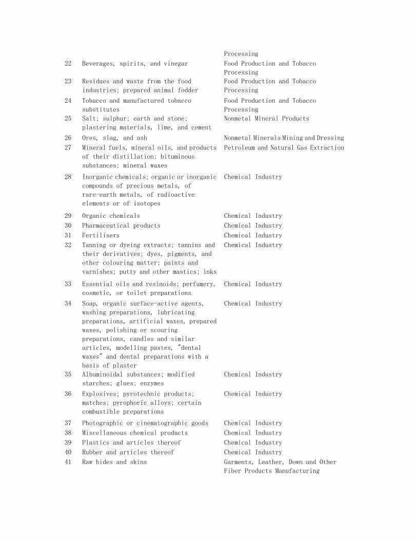
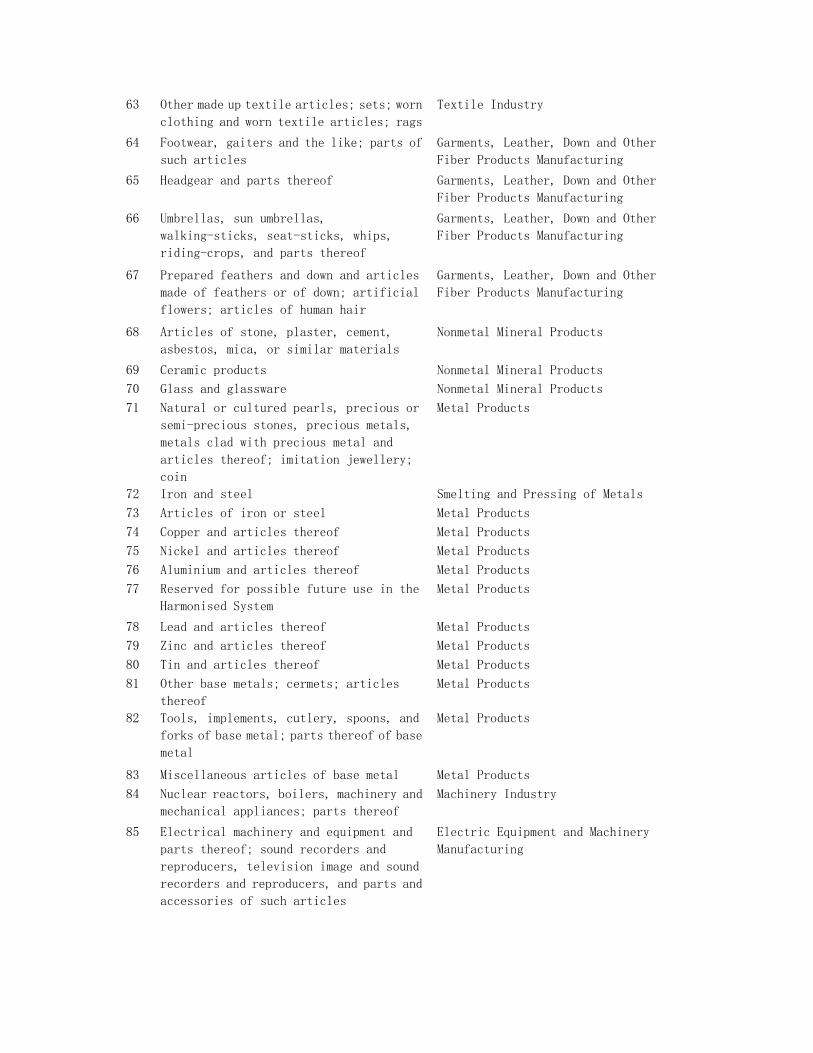
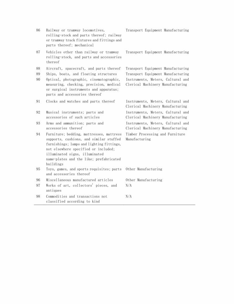
Exports ( E ) and imports ( M ) are taken from the China Trade and External

Economic Statistical Yearbook for 2001 through 2010 (40). Since 1992, China has

utilized a harmonized coding system to code, classify, and conduct statistical analyses

for import and export commodities. The coding system includes information for 22

sections and 98 chapters, which is projected here to the 42 sectors for IOA (see Table

S7).

Figure S2a presents GDP, export and import volumes of China from 2000 to

2009 needed for emission analysis.

3. Monte Carlo method for uncertainty evaluation

As evident from the analysis above, the calculation EEE and EAI is subject to

errors of varying magnitudes in emission factors, activity rates, IOTs, and other

economic data. The resulting emission uncertainties are estimated using the Monte

Carlo approach with at least 10,000 simulations for any given species depending on

the convergence efficiency. For EEI, additional errors are incorporated in uncertainty

analysis upon results from the Monte Carlo simulations to account for the simplified

conversion from EAI to EEI in the present study (see section 5).

A critical procedure of Monte Carlo simulations is specifying probability

distributions of errors in individual input parameters. Based on a review of previous

studies, errors in most parameters are assumed to follow zero-mean normal

distributions, except for emission factors of BC and OC for which a lognormal

distribution is adopted (18).

Errors in each element of A ( Aij) are assumed to have a 95% confidence

interval (CI) of [-10%, 10%] (relative to Aij) for 2000, 2002, 2005 and 2007. For

other years with no direct official data, errors from interpolation shown in section

1.4.1 are added (in quadrature) to account for the impact of rapidly changing

industrial structure.

Errors in export and import volumes are assumed to have a CI of [-10%, 10%],

since they have been reorganized to match the sectors in the IOTs. The CI of errors in

GDP data is assigned to be [-5%, 5%].

For errors in fossil fuel consumption data, the CI is set at [-10%, 10%] for power

plants, [-20%, 20%] for the industrial sector and residential liquid fuel use, and [-33%,

33%] for residential coal use (34). The error assignment accounts for differences

between the national-level (used here) and the provincial-level economic statistics.

The CI is taken to be [-15%, 15%] and [-30%, 30%] for errors in VP and VM,

respectively.

The CI of errors in emission factors is set at [-10%, 10%] for CO2, [-20%, 20%]

for SO2, [-30%, 30%] for NOx and [-70%, 70%] for CO (9, 10). For emission factors

of BC and OC, lognormal distributions are adopted here with uncertainty estimates

following Lu et al. (18) for individual sectors.

4. Total emissions in China

Figure S3 shows the trend of total emissions in China from 2000 to 2009 for four

main sectors: power plants, industry, transportation and residential use.

In China, CO2 emissions are derived mainly from coal and oil combustion in the

power and industrial sectors, with a minor contribution from natural gas usage. As

shown in Fig. S3, CO2 emissions increased from 2000 to 2009 at a rate of about 9%

per year along with the economic booming and resulting growth in energy

consumption (12). Our results are slightly larger than the IEA estimate (12). The

differences are less than 5% throughout the years, and are attributed mainly to the

industrial sector. A likely factor is use of oils in the refinery industry assumed here to

be combusted due to lack of detailed information.

Trend of SO2 emissions differs between two time periods (Fig. S3). From 2000

to 2006, emissions increased dramatically as a result of the rapidly increasing energy

consumption and coal use. After 2006, SO2 emissions began to decrease resulting

primarily from the application of FGD systems, the phase-out of small and

highly-emitting power generation units, and the economic recession (section 1.4.3).

The FGD systems alone have reduced emission factors in power plants by about 69%

from 2000 to 2009. Our results are within 10% of Zhang et al. (10) and Lu et al. (18).

Note that the national-level statistics are employed here for activity rates, differing

from the provincial-level data used by Zhang et al. (10).

Emissions of NOx increased rapidly from 2000 to 2008 (averaged at 8.4% per

year; see Fig. S3), with an increment by 26% from 2005 to 2008 close to constraints

from satellite measurements at 27-33% (41). The growth is driven mainly by

explosive growth in the power and industrial sectors and the use of precalciner kilns

for cement production with high emission factors (10). The rapidly increasing

penetration of fluidized-bed furnaces since 2007 also had a large impact on NOx

emissions from industrial boilers. Emissions in the transportation sector grew slowly

because of the rapidly expanding vehicle fleet compensated substantially by the effect

of continuously enhanced vehicle emission standards (25, 37). After 2008, emission

growth slowed down mainly reflecting the global financial crisis (37, 41). The amount

of emissions for 2006 is about 20% lower than the constraint from satellite

measurements (42) due to errors in the bottom-up calculation and/or errors embedded

in the satellite-based constraint process (25, 43). Vehicle emissions are likely

overestimated over 2007 – 2009 since emission factors are fixed at the 2006 level in

lack of further information.

CO is emitted mainly from industrial combustion, residential burning and vehicle

exhaust with relatively low combustion efficiency. Emissions of CO increased at a

relatively slow pace of 5% per year from 2000 to 2005 (Fig. S3), despite the rapid

economic and industrial development. This is in part because of the increasing

penetration of precalciner kilns with much smaller emission factors than previously

dominant shaft kilns. Other factors include the increasing new combustion boilers

with by-pass gas recycling devices and new iron/steel factories with lower emission

factors in the non-combustion processes (see section 1.4.3 and Table S5). In the

residential sector, emissions of CO were relatively stable over the years due to

reductions in emission factors compensated by enhancements in activity rates. CO

emissions declined slightly since 2006 in the transportation sector. Overall, our results

are lower than Zhang et al. (10) by about 13% in 2001 and 3% in 2006.

BC is produced mostly from incomplete combustion in small and

low-temperature facilities. The residential sector contributes about 49-55% of BC

emissions in China across the years (Fig. S3). Overall, BC emissions increased

slightly from 2000 to 2009, in close agreement with Lu et al. (18) with differences

less than 5% for individual years. The trend is determined by increasing activity rates

compensated in part by decreasing emission factors. From 2000 to 2008, GDP grew

by 177% while emission factors for industrial and residential coal use decreased by

64% and 34% for the same period, respectively (18).

OC exhibited an emission trend similar to BC. As the dominant source, the

residential sector accounted for 72 – 79% of OC emissions during 2000 – 2009.

Throughout the years, the contribution increased from the transportation sector and

decreased from the industrial sector, as a result of increasing vehicle numbers

concurrent with decreasing emission factors in industrial coal use. The estimate here

is close to Lu et al. (18) with differences less than 10% for all years.

5. Emission intensity and trade-induced emissions

5.1 Emission intensity

Emission intensity ( F) in 2002, 2005 and 2007 are shown in Tables S8-9 for

CO2 and air pollutants from various sectors. Among the non-residential sectors,

emissions are most intensive in the electricity/heating/water industry, building

materials and non-metal mineral products industry, transportation and metal products

industry.

Note that the calculation of emission intensity is affected by the use of economic

outputs in monetary units subject to inflation over the years. The effect is partially

accounted for by using the PPI for inflation adjustment. Furthermore, F is an

intermediate term in deriving trade-related emissions

( EEE= ( / )e e

i i i i ii iF X PX X and EAI= ( / )m m

i i i i ii iF X PX X , where both

X e and Xm

are affected by inflation), thus the inflation-induced uncertainties likely

have an insignificant impact on trade-related emissions.

5.2. Trade-induced emissions

5.2.1 Emissions embodied in exports (EEE)

Figure S5 presents EEE of CO2 and air pollutants from 2000 to 2009. For all

species, EEE increased dramatically from 2001 to 2007 as a result of increasing

X e by a factor of about four (Fig. S2). Since 2007, EEE reduced generally because

both of decreasing X e associated with the global final crisis (Fig. S2) and of

decreasing emission intensity due to technology development and environmental

legislation (see sections 2.3 and 3).

Figure S5 also specifies emissions embodied in exports to the U.S., European

Union (EU), Japan, and the rest countries. For a given year, the fractions of EEE

attributable to exports to a particular trade partner were relatively consistent among

the species. Exports to the U.S. accounted for 21% of the total EEE over 2000 – 2007.

The portion for EU increased from 16% in 2000 to 20% in 2007. The contributions of

exports to the U.S. and EU declined in 2008 and 2009 as a result of the financial crisis

and shrinking demand. Japan accounted for about 15% of the total EEE during 2000 –

2003, reducing since to about 7% in 2009. For all species, the three regions accounted

for half of the EEE and almost 15% of total emissions in China for CO2 and SO2.

5.2.2 CO2 emissions embodied in exports (EEE) and comparison with previous studies

EEE of CO2 increased from 697 Tg in 2001 to 2283 Tg in 2007 (by a factor of

328%) and then declined rapidly to 1608 Tg by 2009, primarily as a result of the

varying X e. Meanwhile, the emission intensity of CO2 was relatively stable over the

years (see Tables S8-9).

Figure S4a compares our results with Weber et al. (17), Liu et al. (44) and Peters

et al. (6). Unlike other studies, Liu et al. (44) did not use the IOA approach. Rather,

they calculated the EEE by multiplying the export values by the average emission

intensity. Our results are slightly higher than Peters et al. (6), especially after 2004.

This is mainly because of the rapid structural changes in supply chain explicitly taken

into account here. Peters et al. (6) employed the IOT of 2002 adopted from the Global

Trade Analysis Project 7 (GTAP-7) to calculate the EEE during 2003 – 2008. Here a

test is conducted to estimate the EEE for 2000 – 2009 using the IOT of 2002,

resulting in emissions similar to Peters et al. (6).

Figure S4b further compares emissions embodied in Chinese exports to the U.S.

(EEE-U.S.) to previous estimates by Peters et al. (6), Shui et al. (45) and Du et al. (46).

Our results are consistent with Peters et al. (6), especially when accounting for the

structural change in supply chain considered here. Results from Shui et al. (45) are

much larger due primarily to the use of different export data (Fig. S4b). Shui et al. (45)

employed data from the U.S. Census Bureau providing much higher values than the

Chinese National Bureau of Statistics adopted here. Based on the U.S. dataset,

Chinese exports amounted to 102.280 billion USD in 2001, about 90% higher than the

Chinese statistics. The discrepancy is attributed to the different official definitions of

exports and imports, particularly when accounting for Chinese exports to the U.S. via

a third party. If the U.S. statistics were used here, our results would be close to Shui et

al. (45) in 2000 – 2001 with some remaining differences in 2002 – 2003 for reasons

that are currently unclear (see Fig. S4b). Du et al. (46) used the same economic

statistics as the present study but suggested EEE-U.S. to be about twice as much as

our results and Peters et al. (6). According to Du et al. (46), EEE-U.S. accounted for

about 12% of total Chinese emissions in 2007, implying a value of 6721 Tg for total

emissions that is about 10% higher than the IEA estimate (12) and about 8% higher

than our results. This however cannot fully explain the large differences in EEE-U.S.

and warrant further investigation.

5.2.3 Air pollutants embodied in exports (EEE)

As shown in Fig. S5, EEE of SO2 increased from 4.8 Tg in 2001 to 12.4 Tg in

2006 (by a factor of 257%) with a slight increase from 2006 to 2007. The rate of

increase is smaller than CO2 attributed mainly to the dramatically decreasing emission

intensity after 2004 with the implementation of FGD systems (Table S8). After 2007,

EEE of SO2 declined due to continuously decreasing emission intensity accompanied

by declining exports.

EEE of NOx increased from 2.2 Tg in 2000 to 7.1 Tg in 2007 (by a factor of

322%), close to the trend of EEE of CO2. The growth was driven mainly by the

economic and industrial growth. Although emission intensity of NOx increased

rapidly in the building materials and non-metal products industries, these sectors serve

dominantly for domestic use with a lesser influence on export-related emissions. For

the power and transportation sectors, emission intensity of NOx declined faster than

that for CO2 due to installation of LNBs and vehicle emission control technologies,

respectively. After 2007, EEE of NOx declined along with decreasing exports.

For CO, EEE increased from 14.4 Tg in 2001 to 39.7 Tg in 2007 (by a factor of

280%), at a rate lower than CO2 due to rapidly decreasing emission intensity (Table

S8). After 2007, reductions in emission intensity and exports resulted in significant

declines of EEE with a total of only 24.9 Tg in 2009.

For BC and OC, residential use is the main emission source and is relatively

independent of exports. In other sectors, emission intensity decreased significantly

over the years, partially compensating for the effect of rapidly growing export volume.

As a result, EEE of BC and OC increased from 2001 to 2007 at a rate smaller than

other species. For BC, EEE increased continuously from 125 Gg in 2001 to 291 Gg in

2007 and then declined gradually to a value of 187 Gg in 2009. EEE of OC exhibited

a similar trend.

5.2.4 Emissions avoided by imports (EAI) and emission embodied in imports (EEI)

During 2000 – 2009, China imported large quantities of machines, equipment,

chemical/metal products, and other goods. As shown in Fig. S2, the sectoral sum of

Xm continued to grow until disrupted by the global recession in 2008 – 2009. There

was a sharp increase between 2002 and 2004 mainly because of enhanced imports of

iron, steels and other industrial materials.

Between 2000 and 2002, EAI were relatively stable for most species (Fig. S5) as

a result of slowly increasing Xm (Fig. S2) compensated by slowly decreasing

emission intensity (Tables S8-9). In the following two years, increases in Xm

(particularly in the steel, iron and coke industries) overcompensated for the effect of

declining emission intensity, resulting in rapid growth of EAI. From 2005 to 2007,

EAI decreased gradually for SO2, BC, OC and CO due to reductions in emission

intensity outweighing the effect of increasing import volume (Fig. S5). On the

contrary, EAI for CO2 and NOx increased gradually since the emission intensity

declined more slowly. After 2007, both Xm and F decreased (Fig. S2 and Tables

S8-9) resulting in sharp decline of EAI for all species.

The fractions of EAI with respect to individual trade partners are similar for all

species. Japan accounted for 21% of EAI in 2000 decreasing gradually to 16% in

2009. The U.S. and EU contributed 8% and 13%, respectively, averaged over the

years.

EEI are lower than EAI by a factor of 3 – 5 during 2000-2009 (Fig. S5)

reflecting the high emission/GDP ratio of China relative to its trade partners on

average (Table S1). EEI of CO2 derived here are close to the multi-regional IOA

estimate by Peters et al. (6) with a small difference of about 10% averaged over 2002

– 2008.

The U.S., EU and Japan each contributed about 6% to EEI of CO2 averaged over

the years. Their total contribution (18%) was about half as much as that for EAI. For

air pollutants, the fractions of EEI with respect to individual trade partners vary across

the species due to differences in the emission/GDP ratio (Table S1). Japan, EU and

the U.S. together accounted for 13% of EEI for NOx and 4 – 8% for other species.

Difference between production-based Chinese anthropogenic emissions and

consumption-based emissions are calculated as EEE subtracted by EEI (6). This

quantity is presented in the main text as the emissions embodied in trade (EET).

5.3 Uncertainties in total and trade-induced emissions

Averaged over 2000 – 2009, the Monte Carlo simulations suggest uncertainties

in total emissions (relative to a 95% confidence interval) for CO2, SO2, NOx, CO, BC

and OC to be -15% to 15%, -19% to 19%, -31% to 31%, -64% to 64%, -40 % to 80%

and -41% to 90%, respectively. Uncertainties are asymmetric for BC and OC,

reflecting the assumed lognormal distribution for errors in emission factors (18, 39).

Averaged over the years, uncertainties in EEE of CO2, SO2, NOx, CO, BC, and

OC are estimated to be -15% to 15%, -17% to 17%, -27% to 27%, -45% to 45%,

-35 % to 51%, -41% to 60%, respectively. They are smaller than those for total

emissions because of the weaker influence from the residential sector that is subject to

much larger errors than other source types.

Uncertainties for EAI are similar to EEE. For EEI, emissions for CO2 differ from

Peters et al. (6) by ~ 10% averaged over 2002 – 2008 (Fig. S4), which amount is

added (in quadrature), in deriving the overall uncertainty here, to account for errors

induced by the analysis based mainly on Chinese data instead of performing a

multi-regional input-output calculation (section 1.1.1). For air pollutants, an

additional error at 50% (instead of 10% as for CO2) is assumed concerning

differences in the effect of economic structure and technology level between CO2 and

air pollutants as well as interannual variability in emission intensity of China relative

to that of other countries. The resulting total uncertainty ranges from 52% to 74% for

various pollutants (Table S10).

6. GEOS-Chem simulations to analyze impacts of international trade on global

atmospheric environment

The international trade, including both exports and imports, has significant

consequences on air quality in China and downwind regions. The impacts are

evaluated in this section through a series of simulations using the GEOS-Chem CTM.

GEOS-Chem (version 8-03-02;

http://wiki.seas.harvard.edu/geos-chem/index.php/MainPage) is driven by the

assimilated meteorological fields of GEOS-5 taken from the National Aeronautics and

Space Administration (NASA) Global Modeling and Assimilation Office (GMAO). It

is run with the full Ox−NOx−CO−VOC−HOx chemistry and online calculation for

various aerosols (sulfate, nitrate, ammonium, BC, OC, sea salt and dust) on the 2.5°

long x 2° lat grid with 47 vertical layers. The non-local scheme is used to simulate

vertical mixing in the planetary boundary layer (PBL)(47, 48).

Natural emissions are specified in Lin (2012) (42). Global anthropogenic

emissions are taken from the EDGAR database, which are replaced by various

regional inventories over the U.S. (NEI05;

http://www.epa.gov/ttn/chief/net/2005inventory.html#inventorydata), Canada (CAC;

http://www.ec.gc.ca/pdb/cac/cac_home_e.cfm), Mexico (BRAVO (49)) and Europe

(EMEP (13)). Anthropogenic emissions in Asia are taken from the INTEX-B

inventory as representative of 2006 (10) for various species including NOx, CO,

non-methane volatile organic compounds (VOC), SO2, BC and OC; and the

associated seasonal and diurnal variability is described in Lin (2012) (42). Over China,

the INTEX-B emissions are replaced by our estimate for the same year for SO2, NOx,

CO, BC and OC, as detailed below.

Model simulations require information on the spatial and seasonal distributions

of emissions from individual sectors. The spatiotemporal distributions of total

emissions are available from the INTEX-B dataset (10), specified for four major

sectors: power plants, industry, transportation and residential use. Spatial distributions

of EEE, EAI and EEI are much more difficult to obtain due to lack of information on

source areas of raw/intermediate/final products and domestic transportation related to

exports and imports. The seasonality of trade-related emissions is also difficult to

derive in lack of relevant economic statistics.

For the power and transportation sectors, differences in spatial distribution are

likely small between emissions related to exports and emissions resulting from

production/transportation of goods for domestic consumption. Spatial differences are

larger for the industrial sector since the industrial outputs in some regions may rely

more on export demand than those in other regions. In lack of detailed information, it

is assumed here that EEE exhibit the same spatial distribution as total emissions

specified in the INTEX-B dataset. Similar assumptions are implemented for the

seasonality of EEE and for the spatiotemporal distributions of EAI and EEI. Further

research is required to better constrain the spatiotemporal variability of trade-induced

emissions.

Six simulations, differentiating mostly in Chinese anthropogenic emissions, are

conducted from December 2005 through 2006, using initial conditions provided from

previous spin-up simulations starting from January 2004. Emissions are perturbed for

SO2, NOx, CO, BC and OC; emissions of VOC are generally kept unchanged unless

stated otherwise. The base simulation (Simulation 1) is driven by total emissions in

China from anthropogenic sources derived in this study. The following two

simulations subtract total Chinese emissions by EEE (Simulation 2) and EEE related

to production of goods for consumption in the U.S. (about 21% of the total EEE;

Simulation 3), respectively, to quantify the impacts of trade-induced emissions on

regional air quality and global transport.

Simulation 4 subtracts the total Chinese emissions by the amount of reduced

EEE if the U.S. industrial and emission control technologies were applied to China

(see Sect. 7 for discussion of their differences). Comparing Simulation 4 and

Simulation 3 shows the impact of improved technologies on Chinese EEE and the

consequent global transport.

Simulation 5 incorporates assumed EEE of VOC at 20% of Chinese total for

comparison with Simulation 2; it better simulates the impact of EEE on the ozone

formation. Specifically, Eq. 15 is used to calculate EEE of VOC. In deriving emission

intensity for each sector, however, emissions in 2010 allocated to eight sectors by

Klimont et al.(50) are re-distributed to the 42 sectors here. Differences in emission

factors are neglected between sectors here that are mapped to the same sector in

Klimont et al., due to lack of detailed information. As a result, the EEE of NOx, VOC

and CO together enhance the annual mean surface ozone concentrations by 0-2% over

the North China Plain (Fig. S6). Meanwhile, ozone concentrations outside of China

are enhanced by the Chinese EEE of NOx and CO, whether or not the EEE of VOC

are considered in the simulations (comparing Fig. 2b and Fig. S6).

Simulation 6 is conducted for comparison with Simulation 3. In addition to the

perturbation of Chinese emissions as in Simulation 3, it assumes an increase of

pollutant emissions in the U.S. if goods imported from China were produced in the

U.S. instead.

7. Understanding the high emission/GDP ratio of China relative to the U.S.

level and impacts of less advanced technology level

Per unit of GDP in 2006, China emits 4.9 times as much CO2 and 6.0 – 32.5

times as much air pollution as the U.S. (Table S1). The relatively high emission/GDP

ratio of China is caused in part by its manufacture-dominant economic structure. In

2006, its manufacturing industry contributes 43% of GDP (11), compared to 12% for

the U.S. (http://www.bea.gov/industry/iedguide.htm#gdpia_ou). Chinese economy

also relies mostly on coal as energy source with relatively low energy efficiency. In

addition, emission factors for air pollutants are relatively high in China with less

advanced emission control technologies. China emits 8.12 grams of SO2, 4.05 grams

of NOx and 1.65 grams of CO for a kilowatt hour (kWh) of coal-fired electricity

generation in 2005, about 1.6-7.0 times as large as the U.S. level (Table S11). By

comparison, emission factors of CO2 differ only by 7% between China and the U.S.

(Table S11) due to lack of decarbonizing processes in both countries.

Differences in the emission/GDP ratio between China and the U.S. (Table S1)

are attributed to economic structure, energy efficiency and emission control

technology. To quantify the combined effect of energy efficiency and emission

control technology, differences in the emission/GDP ratio for CO2 between the two

countries are assumed to be caused solely by differences in their economic structures

(i.e., differences in energy efficiency and emission factor are negligible for CO2 for

any given combustion or non-combustion process, as demonstrated above for the

coal-fired power industry). As such the combined effect of energy efficiency and

emission control technology can be derived by dividing the ratio between China and

the U.S. for emissions per GDP of a given short-lived air pollutant by the ratio for

CO2. While the estimate here is relatively rough, it does provide some insight into the

differences in energy efficiency and emission controls between the two countries.

Table S1. Emission/GDP of China divided by that of trade partners in 2006 a

Pollutants China/US China/EU China/Japan b China/Others China/world

CO2 4.9 7.0 10.2 2.5 3.3

SO2 12.4 17.7 75.3 3.5 4.9

NOx 6.0 8.1 24.4 2.7 3.6

CO 9.9 23.0 161.0 3.0 4.5

BC 22.5 15.8 58.5 3.8 5.3

OC 32.5 22.2 179.8 3.6 5.2

a The quantity of ‘emission/GDP’ is closely related to the overall emission intensity

defined as emissions per unit of total monetary outputs. Data sources: World Bank for

GDP and population (http://data.worldbank.org/); this study for emissions of all

pollutants in China; Bond et al. (15) for BC and OC emissions in other countries; NEI05

for SO2, NOx and CO emissions in the U.S. (http://www.epa.gov/ttnchie1/trends/); EMEP

for SO2, NOx and CO emissions in the EU

(http://www.ceip.at/webdab-emission-database/); and REAS (14) for SO2, NOx and CO

emissions in Japan.

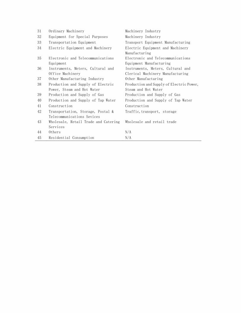
Table S2. Projection of 45 sectors in energy data to the 42 IOT sectors

No. Sector in energy data Sector in IOTs

1 Farming, Forestry, Animal Husbandry,

Fishery and Water Conservancy

Agriculture

2 Coal Mining and Dressing Coal Mining and Processing

3 Petroleum and Natrual Gas Extraction Petroleum and Natural Gas Extraction

4 Ferrous Metals Mining and Dressing Metals Mining and Dressing

5 Nonferrous Metals Mining and Dressing Metals Mining and Dressing

6 Nonmental Minerals Mining and Dressing Nonmetal Minerals Mining and Dressing

7 Other Minerals Mining and Dressing Nonmetal Minerals Mining and Dressing

8 Logging and Transport of Wood and

Bamboo

Agriculture

9 Food Processing Food Production and Tobacco Processing

10 Food Production Food Production and Tobacco Processing

11 Beverage Production Food Production and Tobacco Processing

12 Tobacco Processing Food Production and Tobacco Processing

13 Textile Industry Textile Industry

14 Garments and Other Fibers Products Garments, Leather, Down and Other Fiber

Products Manufacturing

15 Leather, Furs, Down and Related

Products

Garments, Leather, Down and Other Fiber


16 Timber Processing, Bamboo, Cane, Palm

Fiber & Straw Products

Timber Processing and Furniture

Manufacturing

17 Furniture manufacturing Timber Processing and Furniture

Manufacturing

18 Papermaking and Paper Products Papermaking, Printing, Cultural and

Educational Goods Manufacturing

19 Printing and Record Medium

Reproduction

Papermaking, Printing, Cultural and


20 Cultural, Educational and Sports

Articles



21 Petroleum Processing and Coking Petroleum Refining and Coking

22 Raw Chemical Materials and Chemical

Products

Chemical Industry

23 Medical and Pharmaceutical Products Chemical Industry

24 Chemical Fiber Chemical Industry

25 Rubber Products Chemical Industry

26 Plastic Products Chemical Industry

27 Nonmetal Mineral Products Nonmetal Mineral Products

28 Smelting and Pressing of Ferrous Metals Smelting and Pressing of Metals

29 Smelting and Pressing of Nonferrous

Metals

Smelting and Pressing of Metals

30 Metal Products Metal Products

31 Ordinary Machinery Machinery Industry

32 Equipment for Special Purposes Machinery Industry

33 Transportation Equipment Transport Equipment Manufacturing

34 Electric Equipment and Machinery Electric Equipment and Machinery

Manufacturing

35 Electronic and Telecommunications

Equipment

Electronic and Telecommunications

Equipment Manufacturing

36 Instruments, Meters, Cultural and

Office Machinery

Instruments, Meters, Cultural and

Clerical Machinery Manufacturing

37 Other Manufacturing Industry Other Manufacturing

38 Production and Supply of Electric

Power, Steam and Hot Water

Production and Supply of Electric Power,

Steam and Hot Water

39 Production and Supply of Gas Production and Supply of Gas

40 Production and Supply of Tap Water Production and Supply of Tap Water

41 Construction Construction

42 Transportation, Storage, Postal &

Telecommunications Sevices

Traffic,transport, storage

43 Wholesale, Retail Trade and Catering

Services

Wholesale and retail trade

44 Others N/A

45 Residential Consumption N/A

Table S3. Emission factors for main non-combustion industrial processes

Pollutant Process Technology Unit Value

SO2 a

cement production precalciner kiln kg/t-coal 2.9

cement production other rotary kiln kg/t-coal 12.3

cement production shaft kiln kg/t-coal 12.3

CO b

coking machinery kg/t-coke 1.6

coking indigenous kg/t-coke 15.6

sinter production sintering kg/t-sinter 22

iron production blast furnace kg/t-iron 40.5

steel making basic oxygen furnace kg/t-steel 54.2

steel making electric arc furnace kg/t-steel 9

synthetic ammonia coal-based kg/t-NH3 43




brick production tunnel kiln kg/t-coal 150

lime production shaft kiln, beehive kiln kg/t-coal 155.7

NOx c




brick production tunnel kiln kg/t-coal 4.7

lime production shaft kiln, beehive kiln kg/t-coal 1.7

a Collected from Lei et al. (18).

b Collected from Streets et al. (30).

c Collected from Lei et al. (21) and Zhang et al. (25).

Table S4. Mapping between the 42 sectors in IOTs of 2002-2009 and the 17 sectors in

IOTs of 2000-2001

No. Sector in 42-sector IOTs Sector in 17-sector IOTs

1 Agriculture Agriculture

2 Coal Mining and Processing Mining and Quarrying

3 Petroleum and Natural Gas Extraction Coking, Gas and Petroleum Refining

4 Metals Mining and Dressing Mining and Quarrying

5 Nonmetal Minerals Mining and Dressing Mining and Quarrying

6 Food Production and Tobacco Processing Foodstuff

7 Textile Industry Textile, Sewing, Leather and Furs

Products

8 Garments, Leather, Down and Other Fiber


Textile, Sewing, Leather and Furs

Products

9 Timber Processing and Furniture

Manufacturing

Other Manufacturing

10 Papermaking, Printing, Cultural and


Other Manufacturing

11 Petroleum Refining and Coking Coking, Gas and Petroleum Refining

12 Chemical Industry Chemical Industry

13 Nonmetal Mineral Products Building Materials and Non-metal Mineral

Products

14 Smelting and Pressing of Metals Metal Products

15 Metal Products Metal Products

16 Machinery Industry Machinery and Equipment

17 Transport Equipment Manufacturing Machinery and Equipment

18 Electric Equipment and Machinery

Manufacturing

Machinery and Equipment

19 Electronic and Telecommunications

Equipment Manufacturing


20 Instruments, Meters, Cultural and Clerical

Machinery Manufacturing


21 Other Manufacturing Other Manufacturing

22 Waster and Flotsam Other Services

23 Production and Supply of Electric Power,

Steam and Hot Water

Production and Supply of Electric Power,

Heat Power and Water

24 Production and Supply of Gas Coking, Gas and Petroleum Refining

25 Production and Supply of Tap Water Production and Supply of Electric Power,

Heat Power and Water

26 Construction Construction

27 Traffic,transport, storage Transportation, Postal and

Telecommunication Services

28 Post Transportation, Postal and


29 Information transfer, computer services

and software

Transportation, Postal and


30 Wholesale and retail trade Wholesale and Retail Trades, Hotels and

Catering Services

31 Accommodation and Restaurants Wholesale and Retail Trades, Hotels and

Catering Services

32 Banking and Insurance Banking and Insurance

33 Real Estate Trade Real Estate, Leasing and Business

Services

34 Tenancy and business services Real Estate, Leasing and Business

Services

35 Tourism Other Services

36 Scientific research Other Services

37 Compositive technical service Other Services

38 Other social work Other Services

39 Education Other Services

40 Sanitation, social security and social

welfare

Other Services

41 Culture, sports and entertainment Other Services

42 Public management and social organization Other Services

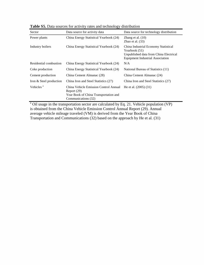
Table S5. Data sources for activity rates and technology distribution

Sector Data source for activity data Data source for technology distribution

Power plants China Energy Statistical Yearbook (24) Zhang et al. (10)

Zhao et al. (33)

Industry boilers China Energy Statistical Yearbook (24) China Industrial Economy Statistical

Yearbook (51)

Unpublished data from China Electrical

Equipment Industrial Association

Residential combustion China Energy Statistical Yearbook (24) N/A

Coke production China Energy Statistical Yearbook (24) National Bureau of Statistics (11)

Cement production China Cement Almanac (28) China Cement Almanac (24)

Iron & Steel production China Iron and Steel Statistics (27) China Iron and Steel Statistics (27)

Vehicles a China Vehicle Emission Control Annual

Report (29)

Year Book of China Transportation and

Communications (32)

He et al. (2005) (31)

a Oil usage in the transportation sector are calculated by Eq. 21. Vehicle population (VP)

is obtained from the China Vehicle Emission Control Annual Report (29). Annual

average vehicle mileage traveled (VM) is derived from the Year Book of China

Transportation and Communications (32) based on the approach by He et al. (31)

Table S6. Emission factors for different fuels used in various sectors

Sector Fuel type Net emission factor (after implementing control measures; kg/GJ)

SO2 a CO b NOx

c BC d OC d

Power Coal 0.20~0.92 0.047~0.052 0.142~0.165 0.0006~0.0012 0.0003~0.0012

Oil 0.20 0.026 0.375 0.0006~0.0008 0.0003~0.0004

Natural gas 0 0.0051 0.0160 0 0

Industry Coal 0.44~0.61 0.33~0.49 0.09~0.11 0.010~0.029 0.009~0.030

Oil 0.19~0.21 0.026 0.307 0.025~0.035 0.008~0.011

Natural gas 0 0.0051 0.0081 0 0

Residential Coal 0.66~0.75 1.05~1.36 0.07~0.08 0.053~0.081 0.12~0.15

Oil 0.14 0.026 0.196 0.058~0.070 0.019~0.022

Biofuel 0.012 2.99 0.08 0.058 0.21

Natural gas 0 0.0051 0.0057 0 0

Transportation On-road gasoline 0.005~0.13 8.61~28.24 0.78~1.29 0.064~0.079 0.019~0.024

On-road diesel 0.002~0.23 1.71~5.33 2.13~2.86 0.011~0.014 0.043~0.073

Off-road oil 0.20~0.25 5.03 1.96 0.030~0.045 0.015~0.020

a Derived from Lu et al. (18).

b Derived from Streets et al. (30) and Zhang et al. (10).

c Derived from Zhang et al. (10, 25).

d Derived from Lu et al. 2011 (18).

Table S7. Mapping between the trade coding chapters and the 42 IOT sectors

No. Trade coding chapter Sector in IOTs

1 Live animals Agriculture

2 Meat and edible offal Agriculture

3 Fish and crustaceans, molluscs, and other

aquatic invertebrates

Agriculture

4 Dairy produce; birds' eggs; natural

honey; edible products of animal origin,

not elsewhere specified or included

Agriculture

5 Products of animal origin, not elsewhere

specified or included

Agriculture

6 Live trees and other plants; bulbs, roots,

and the like; cut flowers and ornamental

foliage

Agriculture

7 Edible vegetables and certain roots and

tubers

Agriculture

8 Edible fruit and nuts; peel of citrus

fruit or melons

Agriculture

9 Coffee, tea, maté, and spices Agriculture

10 Cereals Agriculture

11 Products of the milling industry; malt;

starches; inulin; wheat gluten

Agriculture

12 Oil seeds and oleaginous fruits;

miscellaneous grains, seeds, and fruit;

industrial or medicinal plants; straw and

fodder

Agriculture

13 Lac; gums, resins, and other vegetable

saps and extracts

Agriculture

14 Vegetable plaiting materials; vegetable

products not elsewhere specified or

included

Agriculture

15 Animal or vegetable fats and oils and

their cleavage products; prepared edible

fats; animal or vegetable waxes

Food Production and Tobacco

Processing

16 Preparations of meat, of fish or of

crustaceans, molluscs, or other aquatic

invertebrates


Processing

17 Sugars and sugar confectionery Food Production and Tobacco

Processing

18 Cocoa and cocoa preparations Food Production and Tobacco

Processing

19 Preparations of cereals, flour, starch,

or milk; pastrycooks' products


Processing

20 Preparations of vegetables, fruit, nuts,

or other parts of plants


Processing

21 Miscellaneous edible preparations Food Production and Tobacco

Processing

22 Beverages, spirits, and vinegar Food Production and Tobacco

Processing

23 Residues and waste from the food

industries; prepared animal fodder


Processing

24 Tobacco and manufactured tobacco

substitutes


Processing

25 Salt; sulphur; earth and stone;

plastering materials, lime, and cement

Nonmetal Mineral Products

26 Ores, slag, and ash Nonmetal Minerals Mining and Dressing

27 Mineral fuels, mineral oils, and products

of their distillation; bituminous

substances; mineral waxes

Petroleum and Natural Gas Extraction

28 Inorganic chemicals; organic or inorganic

compounds of precious metals, of

rare-earth metals, of radioactive

elements or of isotopes

Chemical Industry

29 Organic chemicals Chemical Industry

30 Pharmaceutical products Chemical Industry

31 Fertilisers Chemical Industry

32 Tanning or dyeing extracts; tannins and

their derivatives; dyes, pigments, and

other colouring matter; paints and

varnishes; putty and other mastics; inks

Chemical Industry

33 Essential oils and resinoids; perfumery,

cosmetic, or toilet preparations

Chemical Industry

34 Soap, organic surface-active agents,

washing preparations, lubricating

preparations, artificial waxes, prepared

waxes, polishing or scouring

preparations, candles and similar

articles, modelling pastes, "dental

waxes" and dental preparations with a

basis of plaster

Chemical Industry

35 Albuminoidal substances; modified

starches; glues; enzymes

Chemical Industry

36 Explosives; pyrotechnic products;

matches; pyrophoric alloys; certain

combustible preparations

Chemical Industry

37 Photographic or cinematographic goods Chemical Industry

38 Miscellaneous chemical products Chemical Industry

39 Plastics and articles thereof Chemical Industry

40 Rubber and articles thereof Chemical Industry

41 Raw hides and skins Garments, Leather, Down and Other

Fiber Products Manufacturing

42 Articles of leather; saddlery and

harness; travel goods, handbags, and

similar containers; articles of animal

gut

Garments, Leather, Down and Other


43 Furskins and artificial fur; manufactures

thereof



44 Wood and articles of wood; wood charcoal Timber Processing and Furniture

Manufacturing

45 Cork and articles of cork Timber Processing and Furniture

Manufacturing

46 Manufactures of straw, of esparto, or of

other plaiting materials; basketware and

wickerwork


Manufacturing

47 Pulp of wood or of other fibrous

cellulosic material; recovered



48 Paper and paperboard; articles of paper

pulp, of paper or of paperboard



49 Printed books, newspapers, pictures, and

other products of the printing industry;

manuscripts, typescripts and plans



50 Silk Textile Industry

51 Wool, fine or coarse animal hair;

horsehair yarn, and woven fabric

Textile Industry

52 Cotton Textile Industry

53 Other vegetable textile fibres; paper

yarn, and woven fabrics of paper yarn

Textile Industry

54 Man-made filaments; strip and the like of

man-made textile materials

Textile Industry

55 Man-made staple fibres Textile Industry

56 Wadding, felt, and nonwovens; special

yarns; twine, cordage, ropes and cables

and articles thereof

Textile Industry

57 Carpets and other textile floor coverings Textile Industry

58 Special woven fabrics; tufted textile

fabrics; lace; tapestries; trimmings;

embroidery

Textile Industry

59 Impregnated, coated, covered, or

laminated textile fabrics; textile

articles of a kind suitable for industrial

use

Textile Industry

60 Knitted or crocheted fabrics Textile Industry

61 Articles of apparel and clothing

accessories, knitted or crocheted

Textile Industry

62 Articles of apparel and clothing

accessories, not knitted or crocheted

Textile Industry

63 Other made up textile articles; sets; worn

clothing and worn textile articles; rags

Textile Industry

64 Footwear, gaiters and the like; parts of

such articles



65 Headgear and parts thereof Garments, Leather, Down and Other


66 Umbrellas, sun umbrellas,

walking-sticks, seat-sticks, whips,

riding-crops, and parts thereof



67 Prepared feathers and down and articles

made of feathers or of down; artificial

flowers; articles of human hair



68 Articles of stone, plaster, cement,

asbestos, mica, or similar materials

Nonmetal Mineral Products

69 Ceramic products Nonmetal Mineral Products

70 Glass and glassware Nonmetal Mineral Products

71 Natural or cultured pearls, precious or

semi-precious stones, precious metals,

metals clad with precious metal and

articles thereof; imitation jewellery;

coin

Metal Products

72 Iron and steel Smelting and Pressing of Metals

73 Articles of iron or steel Metal Products

74 Copper and articles thereof Metal Products

75 Nickel and articles thereof Metal Products

76 Aluminium and articles thereof Metal Products

77 Reserved for possible future use in the

Harmonised System

Metal Products

78 Lead and articles thereof Metal Products

79 Zinc and articles thereof Metal Products

80 Tin and articles thereof Metal Products

81 Other base metals; cermets; articles

thereof

Metal Products

82 Tools, implements, cutlery, spoons, and

forks of base metal; parts thereof of base

metal

Metal Products

83 Miscellaneous articles of base metal Metal Products

84 Nuclear reactors, boilers, machinery and

mechanical appliances; parts thereof

Machinery Industry

85 Electrical machinery and equipment and

parts thereof; sound recorders and

reproducers, television image and sound

recorders and reproducers, and parts and

accessories of such articles

Electric Equipment and Machinery

Manufacturing

86 Railway or tramway locomotives,

rolling-stock and parts thereof; railway

or tramway track fixtures and fittings and

parts thereof; mechanical

Transport Equipment Manufacturing

87 Vehicles other than railway or tramway

rolling-stock, and parts and accessories

thereof

Transport Equipment Manufacturing

88 Aircraft, spacecraft, and parts thereof Transport Equipment Manufacturing

89 Ships, boats, and floating structures Transport Equipment Manufacturing

90 Optical, photographic, cinematographic,

measuring, checking, precision, medical

or surgical instruments and apparatus;

parts and accessories thereof



91 Clocks and watches and parts thereof Instruments, Meters, Cultural and


92 Musical instruments; parts and

accessories of such articles



93 Arms and ammunition; parts and

accessories thereof



94 Furniture; bedding, mattresses, mattress

supports, cushions, and similar stuffed

furnishings; lamps and lighting fittings,

not elsewhere specified or included;

illuminated signs, illuminated

name-plates and the like; prefabricated

buildings


Manufacturing

95 Toys, games, and sports requisites; parts

and accessories thereof

Other Manufacturing

96 Miscellaneous manufactured articles Other Manufacturing

97 Works of art, collectors' pieces, and

antiques

N/A

98 Commodities and transactions not

classified according to kind

N/A

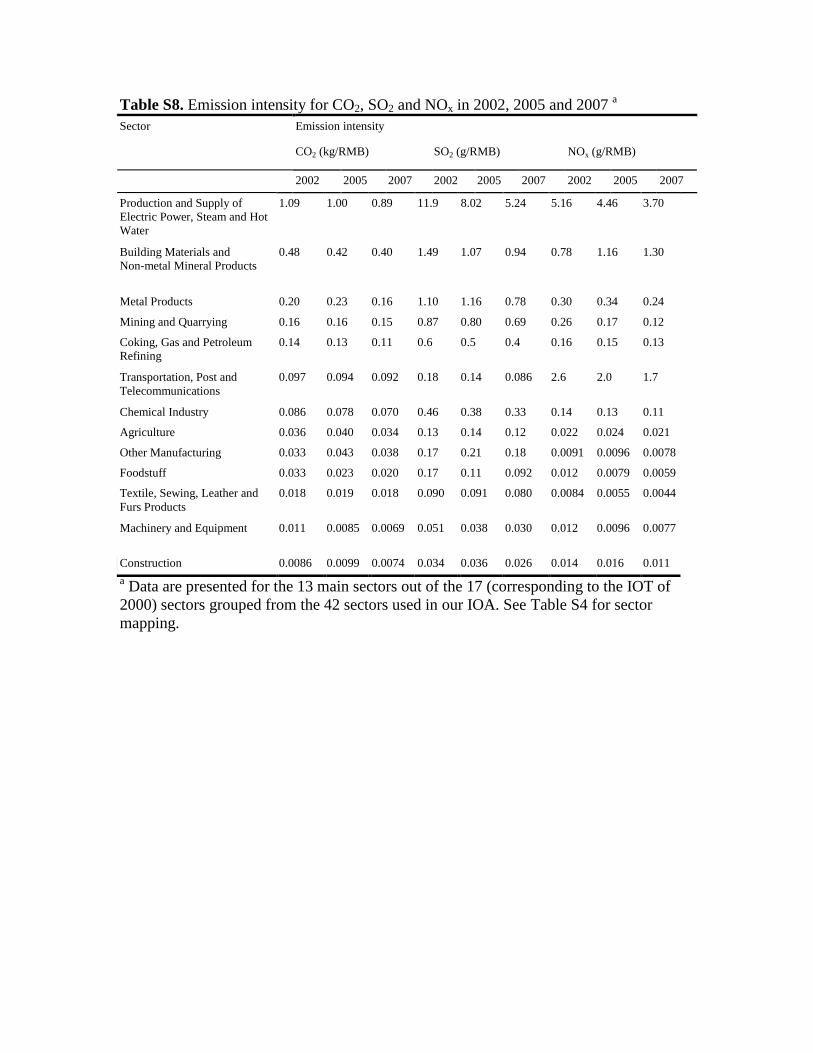
Table S8. Emission intensity for CO2, SO2 and NOx in 2002, 2005 and 2007 a

Sector Emission intensity

CO2 (kg/RMB) SO2 (g/RMB) NOx (g/RMB)

2002 2005 2007 2002 2005 2007 2002 2005 2007

Production and Supply of

Electric Power, Steam and Hot

Water

1.09 1.00 0.89 11.9 8.02 5.24 5.16 4.46 3.70

Building Materials and

Non-metal Mineral Products

0.48 0.42 0.40 1.49 1.07 0.94 0.78 1.16 1.30

Metal Products 0.20 0.23 0.16 1.10 1.16 0.78 0.30 0.34 0.24

Mining and Quarrying 0.16 0.16 0.15 0.87 0.80 0.69 0.26 0.17 0.12

Coking, Gas and Petroleum

Refining

0.14 0.13 0.11 0.6 0.5 0.4 0.16 0.15 0.13

Transportation, Post and

Telecommunications

0.097 0.094 0.092 0.18 0.14 0.086 2.6 2.0 1.7

Chemical Industry 0.086 0.078 0.070 0.46 0.38 0.33 0.14 0.13 0.11

Agriculture 0.036 0.040 0.034 0.13 0.14 0.12 0.022 0.024 0.021

Other Manufacturing 0.033 0.043 0.038 0.17 0.21 0.18 0.0091 0.0096 0.0078

Foodstuff 0.033 0.023 0.020 0.17 0.11 0.092 0.012 0.0079 0.0059

Textile, Sewing, Leather and

Furs Products

0.018 0.019 0.018 0.090 0.091 0.080 0.0084 0.0055 0.0044

Machinery and Equipment 0.011 0.0085 0.0069 0.051 0.038 0.030 0.012 0.0096 0.0077

Construction 0.0086 0.0099 0.0074 0.034 0.036 0.026 0.014 0.016 0.011

a Data are presented for the 13 main sectors out of the 17 (corresponding to the IOT of

2000) sectors grouped from the 42 sectors used in our IOA. See Table S4 for sector

mapping.

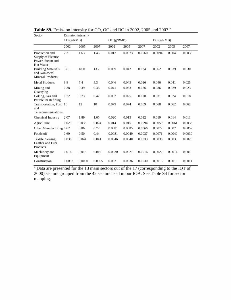
Table S9. Emission intensity for CO, OC and BC in 2002, 2005 and 2007 a

Sector Emission intensity

CO (g/RMB) OC (g/RMB) BC (g/RMB)

2002 2005 2007 2002 2005 2007 2002 2005 2007

Production and

Supply of Electric

Power, Steam and

Hot Water

2.21 1.63 1.46 0.012 0.0073 0.0060 0.0094 0.0049 0.0033

Building Materials

and Non-metal

Mineral Products

37.1 18.0 13.7 0.069 0.042 0.034 0.062 0.039 0.030

Metal Products 6.8 7.4 5.3 0.046 0.043 0.026 0.046 0.041 0.025

Mining and

Quarrying

0.38 0.39 0.36 0.041 0.033 0.026 0.036 0.029 0.023

Coking, Gas and

Petroleum Refining

0.72 0.73 0.47 0.032 0.025 0.020 0.031 0.024 0.018

Transportation, Post

and

Telecommunications

16 12 10 0.079 0.074 0.069 0.068 0.062 0.062

Chemical Industry 2.07 1.89 1.65 0.020 0.015 0.012 0.019 0.014 0.011

Agriculture 0.029 0.035 0.024 0.014 0.015 0.0094 0.0059 0.0061 0.0036

Other Manufacturing 0.62 0.86 0.77 0.0081 0.0085 0.0066 0.0072 0.0075 0.0057

Foodstuff 0.69 0.50 0.44 0.0081 0.0049 0.0037 0.0071 0.0040 0.0030

Textile, Sewing,

Leather and Furs

Products

0.038 0.044 0.041 0.0046 0.0040 0.0033 0.0038 0.0033 0.0026

Machinery and

Equipment

0.016 0.013 0.010 0.0030 0.0021 0.0016 0.0022 0.0014 0.001

Construction 0.0092 0.0090 0.0065 0.0031 0.0036 0.0030 0.0015 0.0015 0.0011

a Data are presented for the 13 main sectors out of the 17 (corresponding to the IOT of

2000) sectors grouped from the 42 sectors used in our IOA. See Table S4 for sector

mapping.

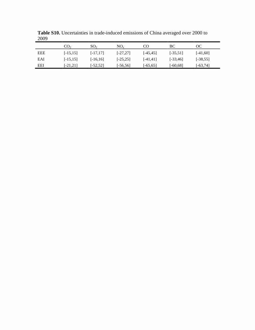
Table S10. Uncertainties in trade-induced emissions of China averaged over 2000 to

2009

CO2 SO2 NOx CO BC OC

EEE [-15,15] [-17,17] [-27,27] [-45,45] [-35,51] [-41,60]

EAI [-15,15] [-16,16] [-25,25] [-41,41] [-33,46] [-38,55]

EEI [-21,21] [-52,52] [-56,56] [-65,65] [-60,68] [-63,74]

Table S11. Emission factors for coal-fired power generation in China and the U.S. Pollutant China (g/kWh) a U.S. (g/kWh) b

CO2 1075 1004

SO2 8.12 5.09

NOx 4.05 1.72

CO 1.65 0.24

a Data are derived from this study.

b Values are calculated based on the NEI05 emission inventory

(http://www.epa.gov/ttn/chief/net/2005inventory.html#inventorydata) and electricity data

from the Energy Information Administration

(http://www.eia.gov/totalenergy/data/annual/showtext.cfm?t=ptb0802c).

Figure S1. Schematic methodology for estimating trade-induced emissions of China.

Unless otherwise specified, data are available over 2000 – 2009. See section 2.1

(Input-output tables) of Material and Methods for interpolation of domestic requirement

matrix and section 2.4 (Economic data) for interpolation of net final demand.

Figure S2. GDP, imports and exports of China over 2000 – 2009. Values are adjusted to

2005 prices based on PPI. (a) GDP, imports and exports. (b) Exported production ( eX )

from 17 sectors and sectoral contributions (in percentage). (c) Imported production ( mX )

from 17 sectors and sectoral contributions (in percentage). The 17 sectors correspond to

the IOT of 2000.

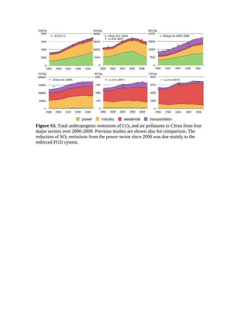
Figure S3. Total anthropogenic emissions of CO2 and air pollutants in China from four

major sectors over 2000-2009. Previous studies are shown also for comparison. The

reduction of SO2 emissions from the power sector since 2006 was due mainly to the

enforced FGD system.

Figure S4. Trade-related anthropogenic emissions of CO2 in China in comparison with

previous studies. (a) EEE. (b) EEE due to exporting goods to the U.S. alone. (c) EEI.

Shaded areas represent the 95% confidence interval derived with the Monte Carlo

simulation in this study.

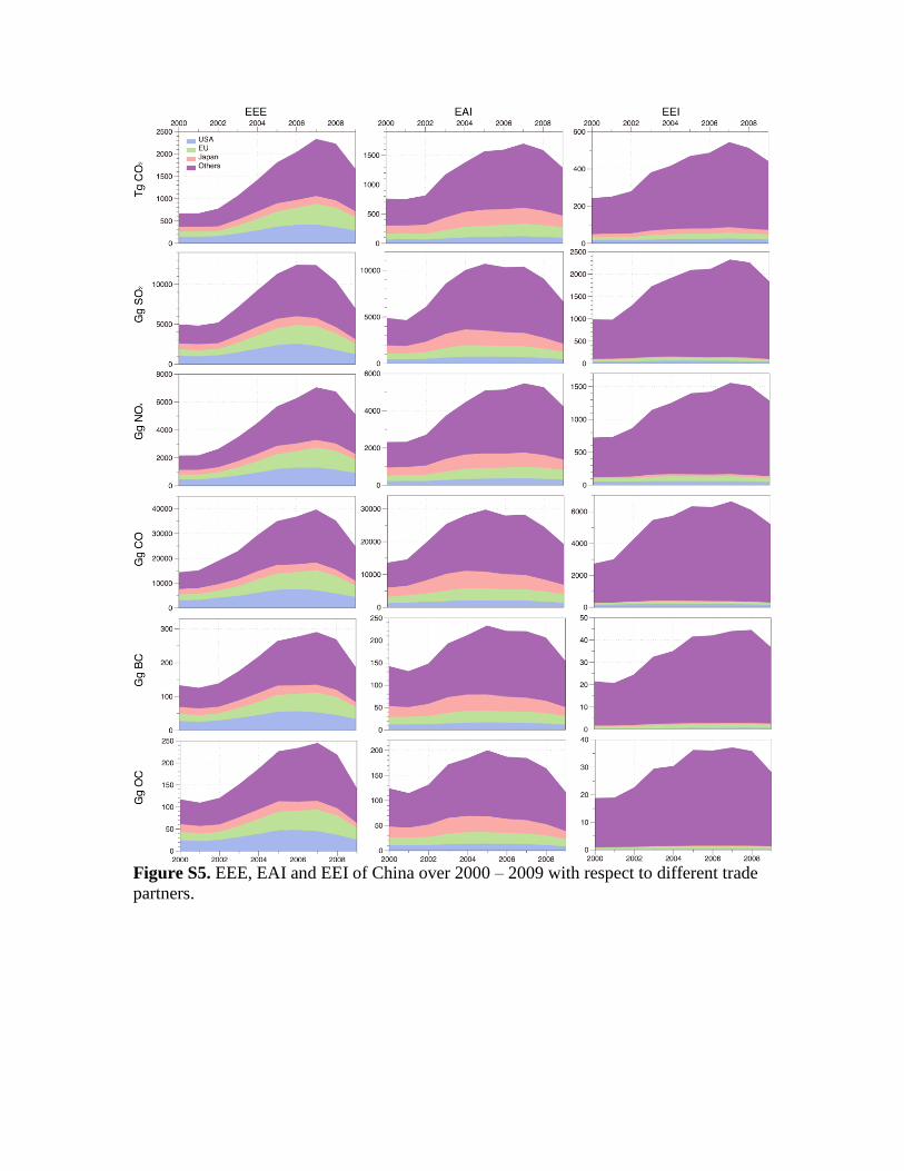
Figure S5. EEE, EAI and EEI of China over 2000 – 2009 with respect to different trade

partners.

Figure S6. Simulated percentage contribution of surface ozone in 2006 from Chinese

EEE of NOx, CO and VOC. Results are shown for annual mean concentrations in the

lowest model layer (0-130 m), presented as (Simulation 1 – Simulation 5) / Simulation 1

in Sect. 6. The color scale is nonlinear to better present the wide range of impacts over

different regions. Compared to results shown in Fig. 2b, the EEE of VOC are accounted

for here, leading to enhanced ozone production efficiency of NOx. The effect is most

evident over the North China Plain.

Figure S7. Simulated percentage contribution of surface air pollution in April 2006 from

Chinese EEE. Results are shown for monthly mean concentrations in the lowest model

layer (0-130 m), presented as (Simulation 1 – Simulation 2) / Simulation 1 in Sect. 6.

The color scale is nonlinear to better present the wide range of impacts over different

regions. Compared to their annual-mean contribution shown in Fig. 2, the contribution

of EEE-related Chinese pollution to the downwind regions is enhanced in spring due to

greater eastward cyclonic activities.

Figure S8. Simulated number of days in 2006 when daily maximum eight-hour average

ozone concentration would not have exceeded the current U.S. standard (75 ppb) but not

for the transport of the EEE-related Chinese air pollution. There are 38 model gridcells

(out of the 217 gridcells constituting the contiguous U.S.) that have such an exceedance

situation, including the gridcells covering the Los Angeles area and many regions in the

eastern U.S. The white color represents one extra day of exceedance. The areas colored in

gray do not have such an exceedance situation.

References

1. Leontief W (1986) Input-output economics (Oxford University Press, USA).

2. Miller RE & Blair PD (1985) Input-Output Analysis: Foundations and Extensions (Prentice-Hall,

Englewood Cliffs, NJ).

3. HIOTCA (1999) Handbook of input-output table compilation and analysis (United Nations).

4. Lin B & Sun C (2010) Evaluating carbon dioxide emissions in international trade of China.

Energy Policy 38(1):613-621.

5. Liu X, Ishikawa M, Wang C, Dong Y, & Liu W (2010) Analyses of CO2 emissions embodied in

Japan-China trade. Energy Policy 38(3):1510-1518.

6. Peters GP, Minx JC, Weber CL, & Edenhofer O (2011) Growth in emission transfers via

international trade from 1990 to 2008. Proceedings of the National Academy of Sciences

108(21):8903.

7. Weber CL & Matthews HS (2007) Embodied environmental emissions in US international trade,

1997-2004. Environmental Science & Technology 41(14):4875-4881.

8. Wiedmann T, Lenzen M, Turner K, & Barrett J (2007) Examining the global environmental

impact of regional consumption activities—Part 2: Review of input–output models for the

assessment of environmental impacts embodied in trade. Ecological Economics 61(1):15-26.

9. Streets D, et al. (2003) An inventory of gaseous and primary aerosol emissions in Asia in the year

2000. J. Geophys. Res 108(D21):8809.

10. Zhang Q, et al. (2009) Asian emissions in 2006 for the NASA INTEX-B mission. Atmospheric

Chemistry and Physics 9(14):5131-5153.

11. CSY (2001~2010) China Statistical Yearbook (China Statistics Press, Beijing).

12. IEA (2011) CO2 emissions from fuel combustion hightlights (2011 Edition) (International Energy

Agency, Paris, France).

13. Auvray M & Bey I (2005) Long-range transport to Europe: Seasonal variations and implications

for the European ozone budget. Journal of Geophysical Research-Atmospheres 110(D11):D11303.

14. Ohara T, et al. (2007) An Asian emission inventory of anthropogenic emission sources for the

period 1980? 2020. Atmospheric Chemistry and Physics Discussions 7(3):6843-6902.

15. Bond TC, et al. (2007) Historical emissions of black and organic carbon aerosol from

energy-related combustion, 1850-2000. Global Biogeochemical Cycles 21(2):Gb2018.

16. Davis SJ & Caldeira K (2010) Consumption-based accounting of CO2 emissions. Proceedings of

the National Academy of Sciences 107(12):5687-5692.

17. Weber CL, Peters GP, Guan D, & Hubacek K (2008) The contribution of Chinese exports to

climate change. Energy Policy 36(9):3572-3577.

18. Lu Z, Zhang Q, & Streets DG (2011) Sulfur dioxide and primary carbonaceous aerosol emissions

in China and India, 1996–2010. Atmos. Chem. Phys 11(18):9839-9864.

19. IPCC (1996) IPCC guidelines for national greenhouse gas inventories. Reference Manual 3.

20. Klimont Z, et al. (2009) Projections of SO2, NOx and carbonaceous aerosols emissions in Asia.

Tellus B 61(4):602-617.

21. Lei Y, Zhang Q, Nielsen C, & He K (2011) An inventory of primary air pollutants and CO2

emissions from cement production in China, 1990–2020. Atmospheric Environment

45(1):147-154.

22. IOTC (2005,2007,2010) Input-Output Table of China (China Statistics Press, Beijing).

23. Xiao L & Xu J (2008) An Empirical Analysis on Real Error of RAS Method. Mathematics in

Practice and Theory.

24. CESY (2001~2010) Chinese Energy Statistical Yearbook (China Statistics Press, Beijing).

25. Zhang Q, et al. (2007) NOx emission trends for China, 1995–2004: The view from the ground and

the view from space. J. Geophys. Res 112:D22306.

26. Guan D, Peters GP, Weber CL, & Hubacek K (2009) Journey to world top emitter: An analysis of

the driving forces of China’s recent CO2 emissions surge. Geophysical Research Letters

36(4):L04709.

27. CISS (2001~2010) China Iron and Steel Statistics (China Steel Industry Association, Beijing).

28. Association CC (2001~2010) China Cement Almanac (China Building Material Press).

29. CVECAR (2010) China Vehicle Emission Control Annual Report. (Ministry of Environmental

Protection of the People's Republic of China).

30. Streets DG, et al. (2006) Revisiting China's CO emissions after the Transport and Chemical

Evolution over the Pacific (TRACE-P) mission: Synthesis of inventories, atmospheric modeling,

and observations. Journal of Geophysical Research 111(D14):D14306.

31. He K, et al. (2005) Oil consumption and CO2 emissions in China's road transport: current status,

future trends, and policy implications. Energy Policy 33(12):1499-1507.

32. YBCTC (2007) Year Book of China Transportation and Communications (China Stat. Press,

Beijing).

33. Zhao Y, et al. (2008) Primary air pollutant emissions of coal-fired power plants in China: Current

status and future prediction. Atmospheric Environment 42(36):8442-8452.

34. Zhao Y, Nielsen C, Lei Y, McElroy M, & Hao J (2011) Quantifying the uncertainties of a

bottom-up emission inventory of anthropogenic atmospheric pollutants in China. Atmospheric


35. Xu Y, Williams RH, & Socolow RH (2009) China's rapid deployment of SO2 scrubbers. Energy

Environ. Sci. 2(5):459-465.

36. Xu Y (2011) Improvements in the operation of SO2 scrubbers in China’s coal power plants.

Environmental Science & Technology.

37. Lin J, et al. (2010) Recent Changes in Particulate Air Pollution over China Observed from Space

and the Ground: Effectiveness of Emission Control. Environmental Science & Technology

44(20):7771-7776.

38. MEP (2001~2010) China statistical yearbook on environment (China Statisitc Press).

39. Bond TC, et al. (2004) A technology-based global inventory of black and organic carbon

emissions from combustion. J. Geophys. Res. 109(D14203).

40. CTEESY (2001~2010) China Trade and External Economic Statistical Yearbook (China Statistics

Press, Beijing).

41. Lin JT & McElroy MB (2011) Detection from space of a reduction in anthropogenic emissions of

nitrogen oxides during the Chinese economic downturn. (Translated from English) Atmospheric

Chemistry and Physics 11(15):8171-8188 (in English).

42. Lin J (2012) Satellite constraint for emissions of nitrogen oxides from anthropogenic, lightning

and soil sources over East China on a high-resolution grid. Atmos. Chem. Phys. 12:2881-2898.

43. Lin JT, McElroy MB, & Boersma KF (2010) Constraint of anthropogenic NOx emissions in China

from different sectors: a new methodology using multiple satellite retrievals. Atmospheric


44. Liu W, Wang Y, & Ye J (2010) CO2 emissions embodied in international trade of China,

1997–2007. in International Conference on Management Science and Engineering - ICMSE

(IEEE), pp 1906-1910.

45. Shui B & Harriss RC (2006) The role of CO2 embodiment in US–China trade. Energy Policy

34(18):4063-4068.

46. Du H, et al. (2011) CO2 emissions embodied in China-US trade: Input-output analysis based on

the emergy/dollar ratio. Energy Policy.

47. Lin JT & McElroy MB (2010) Impacts of boundary layer mixing on pollutant vertical profiles in

the lower troposphere: Implications to satellite remote sensing. Atmospheric Environment

44(14):1726-1739.

48. Lin JT, Youn D, Liang XZ, & Wuebbles DJ (2008) Global model simulation of summertime US

ozone diurnal cycle and its sensitivity to PBL mixing, spatial resolution, and emissions.

Atmospheric Environment 42(36):8470-8483.

49. Kuhns H, Green M, & Etyemezian V (2003) Big Bend Regional Aerosol and Visibility

Observational (BRAVO) Study Emissions Inventory. (Desert Research Institute, Las Vegas, NV

89119).

50. Klimont Z, et al. (2002) Anthropogenic emissions of non-methane volatile organic compounds in

China. Atmospheric Environment 36(8):1309-1322.

51. Statistics NBo (2001, 2006) China Industrial Economy Statistical Yearbook (China Statistic Press,

Beijing).

china s international trade and air pollution in the u.s.€¦ · china’s international trade and...

Documents