chicheng zhang and kamalika chaudhuri university of
TRANSCRIPT
arX
iv:1
510.
0284
7v2
[cs.
LG]
16 O
ct 2
015
Active Learning from Weak and Strong Labelers
Chicheng Zhang∗1 and Kamalika Chaudhuri†1
1University of California, San Diego
October 19, 2015
Abstract
An active learner is given a hypothesis class, a large set of unlabeled examples and the ability tointeractively query labels to an oracle of a subset of these examples; the goal of the learner is to learn ahypothesis in the class that fits the data well by making as fewlabel queries as possible.
This work addresses active learning with labels obtained from strong and weak labelers, where inaddition to the standard active learning setting, we have anextra weak labeler which may occasionallyprovide incorrect labels. An example is learning to classify medical images where either expensive labelsmay be obtained from a physician (oracle or strong labeler),or cheaper but occasionally incorrect labelsmay be obtained from a medical resident (weak labeler). Our goal is to learn a classifier with low erroron data labeled by the oracle, while using the weak labeler toreduce the number of label queries made tothis labeler. We provide an active learning algorithm for this setting, establish its statistical consistency,and analyze its label complexity to characterize when it canprovide label savings over using the stronglabeler alone.
1 Introduction
An active learner is given a hypothesis class, a large set of unlabeled examples and the ability to interactivelymake label queries to an oracle on a subset of these examples;the goal of the learner is to learn a hypothesisin the class that fits the data well by making as few oracle queries as possible.
As labeling examples is a tedious task for any one person, many applications of active learning involvesynthesizing labels from multiple experts who may have slightly different labeling patterns. While a bodyof recent empirical work [28, 29, 30, 26, 27, 12] has developed methods for combining labels from multipleexperts, little is known on the theory of actively learning with labels from multiple annotators. For example,what kind of assumptions are needed for methods that use labels from multiple sources to work, when thesemethods are statistically consistent, and when they can yield benefits over plain active learning are all openquestions.
This work addresses these questions in the context of activelearning from strong and weak labelers.Specifically, in addition to unlabeled data and the usual labeling oracle in standard active learning, we havean extra weak labeler. The labeling oracle is agold standard– an expert on the problem domain – andit provides high quality but expensive labels. The weak labeler is cheap, but may provide incorrect labels
∗[email protected]†[email protected]
1
on some inputs. An example is learning to classify medical images where either expensive labels may beobtained from a physician (oracle), or cheaper but occasionally incorrect labels may be obtained from amedical resident (weak labeler). Our goal is to learn a classifier in a hypothesis class whose error withrespect to the data labeled by the oracle is low, while exploiting the weak labeler to reduce the number ofqueries made to this oracle. Observe that in our model the weak labeler can be incorrect anywhere, and doesnot necessarily provide uniformly noisy labels everywhere, as was assumed by some previous works [8, 24].
A plausible approach in this framework is to learn adifference classifierto predict where the weaklabeler differs from the oracle, and then use a standard active learning algorithm which queries the weaklabeler when this difference classifier predicts agreement. Our first key observation is that this approachis statistically inconsistent; false negative errors (that predict no difference whenO andW differ) lead tobiased annotation for the target classification task. We address this problem by learning instead acost-sensitive difference classifierthat ensures that false negative errors rarely occur. Our second key observationis that as existing active learning algorithms usually query labels in localized regions of space, it is sufficientto train the difference classifier restricted to this regionand still maintain consistency. This process leadsto significant label savings. Combining these two ideas, we get an algorithm that is provably statisticallyconsistent and that works under the assumption that there isa good difference classifier with low falsenegative error.
We analyze the label complexity of our algorithm as measuredby the number of label requests to thelabeling oracle. In general we cannot expect any consistentalgorithm to provide label savings under allcircumstances, and indeed our worst case asymptotic label complexity is the same as that of active learningusing the oracle alone. Our analysis characterizes when we can achieve label savings, and we show that thishappens for example if the weak labeler agrees with the labeling oracle for some fraction of the examplesclose to the decision boundary. Moreover, when the target classification task is agnostic, the number oflabels required to learn the difference classifier is of a lower order than the number of labels required foractive learning; thus in realistic cases, learning the difference classifier adds only a small overhead to thetotal label requirement, and overall we get label savings over using the oracle alone.
Related Work. There has been a considerable amount of empirical work on active learning where multipleannotators can provide labels for the unlabeled examples. One line of work assumes a generative model foreach annotator’s labels. The learning algorithm learns theparameters of the individual labelers, and usesthem to decide which labeler to query for each example. [29, 30, 13] consider separate logistic regressionmodels for each annotator, while [20, 19] assume that each annotator’s labels are corrupted with a differentamount of random classification noise. A second line of work [12, 16] that includes Pro-Active Learning,assumes that each labeler is an expert over an unknown subsetof categories, and uses data to measurethe class-wise expertise in order to optimally place label queries. In general, it is not known under whatconditions these algorithms are statistically consistent, particularly when the modeling assumptions do notstrictly hold, and under what conditions they provide labelsavings over regular active learning.
[25], the first theoretical work to consider this problem, consider a model where the weak labeler is morelikely to provide incorrect labels in heterogeneous regions of space where similar examples have differentlabels. Their formalization is orthogonal to ours – while theirs is more natural in a non-parametric setting,ours is more natural for fitting classifiers in a hypothesis class. In a NIPS 2014 Workshop paper, [21] havealso considered learning from strong and weak labelers; unlike ours, their work is in the online selectivesampling setting, and applies only to linear classifiers androbust regression. [11] study learning frommultiple teachers in the online selective sampling settingin a model where different labelers have differentregions of expertise.
2
Finally, there is a large body of theoretical work [1, 9, 10, 14, 31, 2, 4] on learning a binary classifierbased on interactive label queries madeto a single labeler. In the realizable case, [22, 9] show that a general-ization of binary search provides an exponential improvement in label complexity over passive learning. Theproblem is more challenging, however, in the more realisticagnostic case, where such approaches lead toinconsistency. The two styles of algorithms for agnostic active learning are disagreement-based active learn-ing (DBAL) [1, 10, 14, 4] and the more recent margin-based or confidence-based active learning [2, 31].Our algorithm builds on recent work in DBAL [4, 15].
2 Preliminaries
The Model. We begin with a general framework for actively learning fromweak and strong labelers. Inthe standard active learning setting, we are given unlabelled data drawn from a distributionU over an inputspaceX , a label spaceY = {−1,1}, a hypothesis classH , and a labeling oracleO to which we can makeinteractive queries.
In our setting, we additionally have access to a weak labeling oracleW which we can query interactively.QueryingW is significantly cheaper than queryingO; however, queryingW generates a labelyW drawn froma conditional distributionPW(yW|x) which is not the same as the conditional distributionPO(yO|x) of O.
Let D be the data distribution over labelled examples such that:PD(x,y) = PU(x)PO(y|x). Our goal is tolearn a classifierh in the hypothesis classH such that with probability≥ 1−δ over the sample, we have:PD(h(x) 6= y)≤minh′∈H PD(h′(x) 6= y)+ ε , while making as few (interactive) queries toO as possible.
Observe that in this modelW may disagree with the oracleO anywherein the input space; this isunlike previous frameworks [8, 24] where labels assigned bythe weak labeler are corrupted by randomclassification noise with a higher variance than the labeling oracle. We believe this feature makes our modelmore realistic.
Second, unlike [25], mistakes made by the weak labelerdo not have to be close to the decision boundary.This keeps the model general and simple, and allows greater flexibility to weak labelers. Our analysis showsthat if W is largely incorrect close to the decision boundary, then our algorithm will automatically makemore queries toO in its later stages.
Finally note thatO is allowed to benon-realizablewith respect to the target hypothesis classH .
Background on Active Learning Algorithms. The standard active learning setting is very similar to ours,the only difference being that we have access to the weak oracle W. There has been a long line of work onactive learning [1, 7, 9, 14, 2, 10, 4, 31]. Our algorithms arebased on a style calleddisagreement-basedactive learning (DBAL).The main idea is as follows. Based on the examples seen so far,the algorithmmaintains a candidate setVt of classifiers inH that is guaranteed with high probability to containh∗, theclassifier inH with the lowest error. Given a randomly drawn unlabeled example xt , if all classifiers inVt
agree on its label, then this label is inferred; observe thatwith high probability, this inferred label ish∗(xt).Otherwise,xt is said to be in thedisagreement regionof Vt , and the algorithm queriesO for its label.Vt isupdated based onxt and its label, and algorithm continues.
Recent works in DBAL [10, 4] have observed that it is possibleto determine if anxt is in the disagree-ment region ofVt without explicitly maintainingVt . Instead, a labelled datasetSt is maintained; the labelsof the examples inSt are obtained by either querying the oracle or direct inference. To determine whetheranxt lies in the disagreement region ofVt , two constrained ERM procedures are performed; empirical riskis minimized overSt while constraining the classifier to output the label ofxt as 1 and−1 respectively. If
3
these two classifiers have similar training errors, thenxt lies in the disagreement region ofVt ; otherwise thealgorithm infers a label forxt that agrees with the label assigned byh∗.
More Definitions and Notation. The error of a classifierh under a labelled data distributionQ is definedas: errQ(h) = P(x,y)∼Q(h(x) 6= y); we use the notation err(h,S) to denote its empirical error on a labelled datasetS. We use the notationh∗ to denote the classifier with the lowest error underD andν to denote its errorerrD(h∗), whereD is the target labelled data distribution.
Our active learning algorithm implicitly maintains a(1− δ )-confidence setfor h∗ throughout the algo-rithm. Given a setSof labelled examples, a set of classifiersV(S) ⊆H is said to be a(1− δ )-confidenceset forh∗ with respect toS if h∗ ∈V with probability≥ 1−δ overS.
The disagreement between two classifiersh1 andh2 under an unlabelled data distributionU , denoted byρU(h1,h2), isPx∼U(h1(x) 6= h2(x)). Observe that the disagreements underU form a pseudometric overH .We use BU(h, r) to denote a ball of radiusr centered aroundh in this metric. Thedisagreement regionof asetV of classifiers, denoted by DIS(V), is the set of all examplesx∈X such that there exist two classifiersh1 andh2 in V for whichh1(x) 6= h2(x).
3 Algorithm
Our main algorithm is a standard single-annotator DBAL algorithm with a major modification: when theDBAL algorithm makes a label query, we use an extra sub-routine to decide whether this query should bemade to the oracle or the weak labeler, and make it accordingly. How do we make this decision? We try topredict if weak labeler differs from the oracle on this example; if so, query the oracle, otherwise, query theweak labeler.
Key Idea 1: Cost Sensitive Difference Classifier. How do we predict if the weak labeler differs from theoracle? A plausible approach is to learn adifference classifier hd f in a hypothesis classH d f to determine ifthere is a difference. Our first key observation is when the region whereO andW differ cannot be perfectlymodeled byH d f , the resulting active learning algorithm isstatistically inconsistent. Any false negativeerrors (that is, incorrectly predicting no difference) made by difference classifier leads to biased annotationfor the target classification task, which in turn leads to inconsistency. We address this problem by insteadlearning acost-sensitive difference classifierand we assume that a classifier with low false negative errorexists inH d f . While training, we constrain the false negative error of the difference classifier to be low, andminimize the number of predicted positives (or disagreements betweenW andO) subject to this constraint.This ensures that the annotated data used by the active learning algorithm has diminishing bias, thus ensuringconsistency.
Key Idea 2: Localized Difference Classifier Training. Unfortunately, even with cost-sensitive training,directly learning a difference classifier accurately is expensive. Ifd′ is the VC-dimension of the differencehypothesis classH d f , to learn a target classifier to excess errorε , we need a difference classifier with falsenegative errorO(ε), which, from standard generalization theory, requiresO(d′/ε) labels [6, 23]! Our secondkey observation is that we can save on labels by training the difference classifier in a localized manner –because the DBAL algorithm that builds the target classifieronly makes label queriesin the disagreementregion of the current confidence set forh∗. Therefore we train the difference classifier only on this regionand still maintain consistency. Additionally this provides label savings because while training the target
4
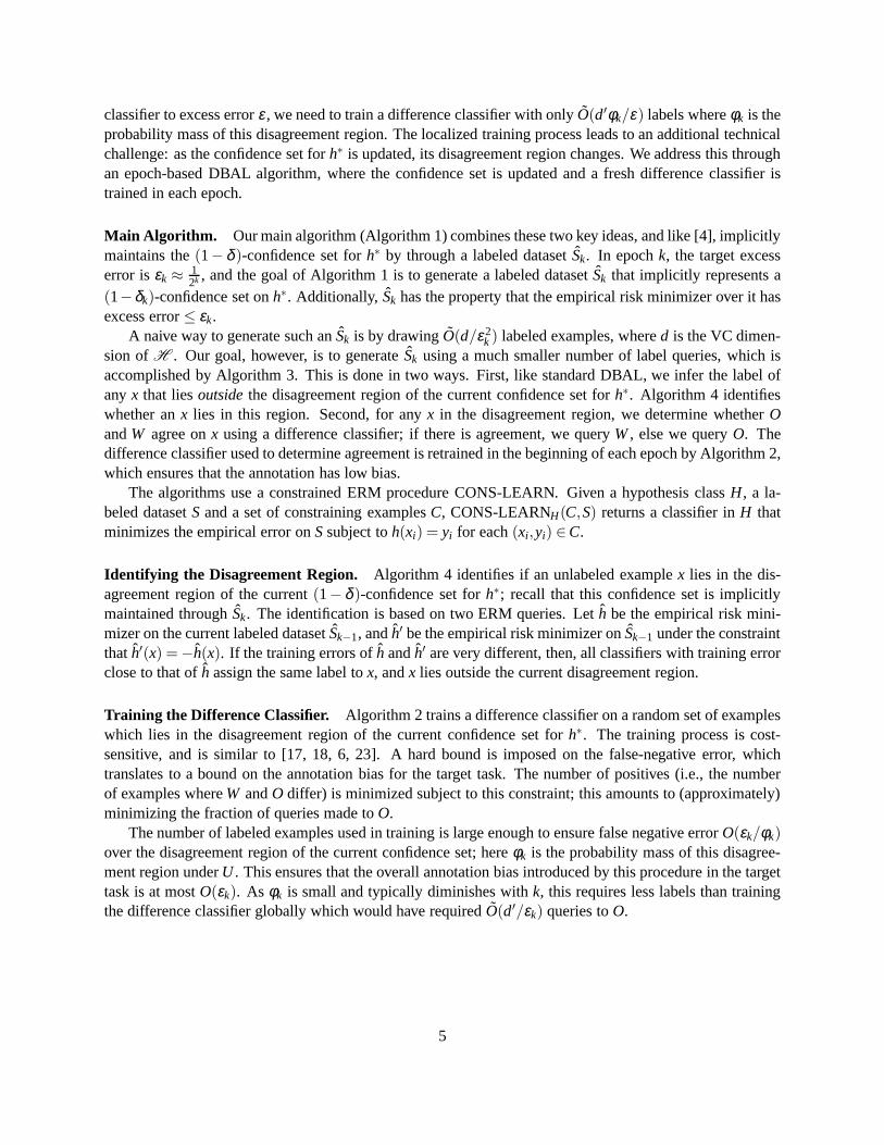
classifier to excess errorε , we need to train a difference classifier with onlyO(d′φk/ε) labels whereφk is theprobability mass of this disagreement region. The localized training process leads to an additional technicalchallenge: as the confidence set forh∗ is updated, its disagreement region changes. We address this throughan epoch-based DBAL algorithm, where the confidence set is updated and a fresh difference classifier istrained in each epoch.
Main Algorithm. Our main algorithm (Algorithm 1) combines these two key ideas, and like [4], implicitlymaintains the(1− δ )-confidence set forh∗ by through a labeled datasetSk. In epochk, the target excesserror isεk ≈ 1
2k , and the goal of Algorithm 1 is to generate a labeled datasetSk that implicitly represents a(1−δk)-confidence set onh∗. Additionally, Sk has the property that the empirical risk minimizer over it hasexcess error≤ εk.
A naive way to generate such anSk is by drawingO(d/ε2k ) labeled examples, whered is the VC dimen-
sion ofH . Our goal, however, is to generateSk using a much smaller number of label queries, which isaccomplished by Algorithm 3. This is done in two ways. First,like standard DBAL, we infer the label ofanyx that liesoutsidethe disagreement region of the current confidence set forh∗. Algorithm 4 identifieswhether anx lies in this region. Second, for anyx in the disagreement region, we determine whetherOandW agree onx using a difference classifier; if there is agreement, we query W, else we queryO. Thedifference classifier used to determine agreement is retrained in the beginning of each epoch by Algorithm 2,which ensures that the annotation has low bias.
The algorithms use a constrained ERM procedure CONS-LEARN.Given a hypothesis classH, a la-beled datasetS and a set of constraining examplesC, CONS-LEARNH(C,S) returns a classifier inH thatminimizes the empirical error onSsubject toh(xi) = yi for each(xi ,yi) ∈C.
Identifying the Disagreement Region. Algorithm 4 identifies if an unlabeled examplex lies in the dis-agreement region of the current(1− δ )-confidence set forh∗; recall that this confidence set is implicitlymaintained throughSk. The identification is based on two ERM queries. Leth be the empirical risk mini-mizer on the current labeled datasetSk−1, andh′ be the empirical risk minimizer onSk−1 under the constraintthath′(x) =−h(x). If the training errors ofh andh′ are very different, then, all classifiers with training errorclose to that ofh assign the same label tox, andx lies outside the current disagreement region.
Training the Difference Classifier. Algorithm 2 trains a difference classifier on a random set of exampleswhich lies in the disagreement region of the current confidence set forh∗. The training process is cost-sensitive, and is similar to [17, 18, 6, 23]. A hard bound is imposed on the false-negative error, whichtranslates to a bound on the annotation bias for the target task. The number of positives (i.e., the numberof examples whereW andO differ) is minimized subject to this constraint; this amounts to (approximately)minimizing the fraction of queries made toO.
The number of labeled examples used in training is large enough to ensure false negative errorO(εk/φk)over the disagreement region of the current confidence set; hereφk is the probability mass of this disagree-ment region underU . This ensures that the overall annotation bias introduced by this procedure in the targettask is at mostO(εk). As φk is small and typically diminishes withk, this requires less labels than trainingthe difference classifier globally which would have required O(d′/εk) queries toO.
5
Algorithm 1 Active Learning Algorithm from Weak and Strong Labelers1: Input: Unlabeled distributionU , target excess errorε , confidenceδ , labeling oracleO, weak oracleW,
hypothesis classH , hypothesis class for difference classifierH d f .2: Output: Classifierh in H .3: Initialize: initial errorε0 = 1, confidenceδ0 = δ/4. Total number of epochsk0 = ⌈log 1
ε ⌉.4: Initial number of examplesn0 = O( 1
ε20(d ln 1
ε20+ ln 1
δ0)).
5: Draw a fresh sample and queryO for its labelsS0 = {(x1,y1), . . . ,(xn0,yn0)}. Let σ0 = σ(n0,δ0).6: for k= 1,2, . . . ,k0 do7: Set target excess errorεk = 2−k, confidenceδk = δ/4(k+1)2.8: # Train Difference Classifier9: hd f
k ← Call Algorithm 2 with inputs unlabeled distributionU , oraclesW andO, target excess errorεk, confidenceδk/2, previously labeled datasetSk−1.
10: # Adaptive Active Learning using Difference Classifier11: σk, Sk← Call Algorithm 3 with inputs unlabeled distributionU , oraclesW andO, difference classi-
fier hd fk , target excess errorεk, confidenceδk/2, previously labeled datasetSk−1.
12: end for13: return h← CONS-LEARNH ( /0, Sk0).
Algorithm 2 Training Algorithm for Difference Classifier
1: Input: Unlabeled distributionU , oraclesW andO, target errorε , hypothesis classH d f , confidenceδ ,previous labeled datasetT.
2: Output: Difference classifierhd f .3: Let p be an estimate ofPx∼U(in disagr region(T, 3ε
2 ,x) = 1), obtained by calling Algorithm 5 withfailure probabilityδ/3. 1
4: LetU ′ = /0, i = 1, and
m=64·1024p
ε(d′ ln
512·1024pε
+ ln72δ) (1)
5: repeat6: Draw an examplexi from U .7: if in disagr region(T, 3ε
2 ,xi) = 1 then # xi is inside the disagreement region8: query bothW andO for labels to getyi,W andyi,O.9: end if
10: U ′ =U ′∪{(xi ,yi,O,yi,W)}11: i = i +112: until |U ′|= m13: Learn a classifierhd f ∈H d f based on the following empirical risk minimizer:
hd f = argminhd f∈H d f
m
∑i=1
1(hd f (xi) = +1), s.t.m
∑i=1
1(hd f (xi) =−1∧yi,O 6= yi,W)≤mε/256p (2)
14: return hd f .
1Note that if in Algorithm 5, the upper confidence bound ofPx∼U (in disagr region(T, 3ε2 ,x) = 1) is lower thanε/64, then we
can halt Algorithm 2 and return an arbitraryhd f in H d f . Using thishd f will still guarantee the correctness of Algorithm 1.
6
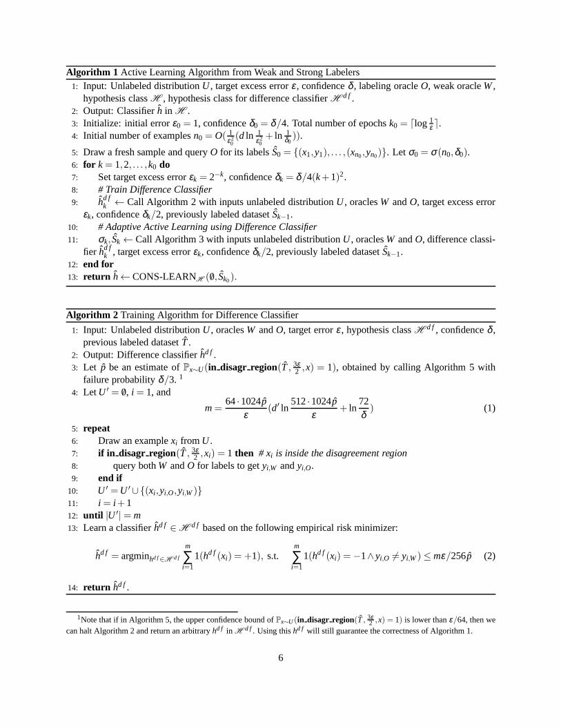
Adaptive Active Learning using the Difference Classifier. Finally, Algorithm 3 is our main active learn-ing procedure, which generates a labeled datasetSk that is implicitly used to maintain a tighter(1− δ )-confidence set forh∗. Specifically, Algorithm 3 generates aSk such that the setVk defined as:
Vk = {h : err(h, Sk)− minhk∈H
err(hk, Sk)≤ 3εk/4}
has the property that:
{h : errD(h)−errD(h∗)≤ εk/2} ⊆Vk ⊆ {h : errD(h)−errD(h
∗)≤ εk}
This is achieved by labeling, through inference or query, a large enough sample of unlabeled data drawnfrom U . Labels are obtained from three sources - direct inference (if x lies outside the disagreement regionas identified by Algorithm 4), queryingO (if the difference classifier predicts a difference), and queryingW. How large should the sample be to reach the target excess error? If errD(h∗) = ν , then achieving anexcess error ofε requiresO(dν/ε2
k ) samples, whered is the VC dimension of the hypothesis class. Asν isunknown in advance, we use a doubling procedure in lines 4-14to iteratively determine the sample size.
Algorithm 3 Adaptive Active Learning using Difference Classifier
1: Input: Unlabeled data distributionU , oraclesW andO, difference classifierhd f , target excess errorε ,confidenceδ , previous labeled datasetT.
2: Output: Parameterσ , labeled datasetS.3: Let h= CONS-LEARNH ( /0, T).4: for t = 1,2, . . . , do5: Let δ t = δ/t(t +1). Define:σ(2t ,δ t) = 8
2t (2d ln 2e2t
d + ln 24δ t ).
6: Draw 2t examples fromU to form St,U .7: for eachx∈ St,U do:8: if in disagr region(T, 3ε
2 ,x) = 0 then # x is inside the agreement region9: Add (x, h(x)) to St .
10: else# x is inside the disagreement region11: If hd f (x) = +1, queryO for the labely of x, otherwise queryW. Add (x,y) to St .12: end if13: end for14: Train ht ← CONS-LEARNH ( /0, St).
15: if σ(2t ,δ t)+√
σ(2t ,δ t)err(ht , St)≤ ε/512 then16: t0← t, break17: end if18: end for19: return σ ← σ(2t0,δ t0), S← St0.
4 Performance Guarantees
We now examine the performance of our algorithm, which is measured by the number of label queries madeto the oracleO. Additionally we require our algorithm to be statisticallyconsistent, which means that thetrue error of the output classifier should converge to the true error of the best classifier inH on the datadistributionD.
7
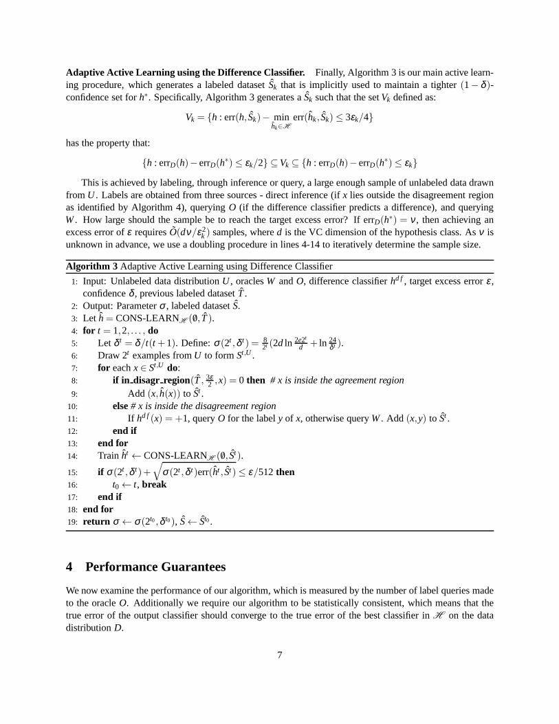
Algorithm 4 in disagr region(S,τ ,x): Test ifx is in the disagreement region of current confidence set
1: Input: labeled datasetS, rejection thresholdτ , unlabeled examplex.2: Output: 1 ifx in the disagreement region of current confidence set, 0 otherwise.3: Train h← CONS-LEARNH ({ /0, S}).4: Train h′x← CONS-LEARNH ({(x,−h(x))}, S}).5: if err(h′x, S)−err(h, S)> τ then # x is in the agreement region6: return 07: else # x is in the disagreement region8: return 19: end if
Since our framework is very general, we cannot expect any statistically consistent algorithm to achievelabel savings over usingO alone under all circumstances. For example, if labels provided byW are thecomplete opposite ofO, no algorithm will achieve both consistency and label savings. We next provide anassumption under which Algorithm 1 works and yields label savings.
Assumption. The following assumption states that difference hypothesis class contains a good cost-sensitivepredictor of whenO andW differ in the disagreement region of BU(h∗, r); a predictor is good if it has lowfalse-negative error and predicts a positive label with lowfrequency. If there is no such predictor, then wecannot expect an algorithm similar to ours to achieve label savings.
Assumption 1. LetD be the joint distribution:PD(x,yO,yW) = PU(x)PW(yW|x)PO(yO|x). For any r,η > 0,there exists an hd f
η ,r ∈H d f with the following properties:
PD(hd fη ,r (x) =−1,x∈ DIS(BU(h∗, r)),yO 6= yW)≤ η (3)
PD(hd fη ,r (x) = 1,x∈DIS(BU(h∗, r)))≤ α(r,η) (4)
Note that (3), which states there is ahd f ∈H d f with low false-negative error, is minimally restrictive,and is trivially satisfied ifH d f includes the constant classifier that always predicts 1. Theorem showsthat (3) is sufficient to ensure statistical consistency.
(4) in addition states that the number of positives predicted by the classifierhd fη ,r is upper bounded by
α(r,η). Noteα(r,η) ≤ PU(DIS(BU(h∗, r))) always; performance gain is obtained whenα(r,η) is lower,which happens when the difference classifier predicts agreement on a significant portion of DIS(BU(h∗, r)).
Consistency. Provided Assumption 1 holds, we next show that Algorithm 1 isstatistically consistent.Establishing consistency is non-trivial for our algorithmas the output classifier is trained on labels frombothO andW.
Theorem 1(Consistency). Let h∗ be the classifier that minimizes the error with respect to D. If Assumption 1holds, then with probability≥ 1−δ , the classifierh output by Algorithm 1 satisfies: errD(h)≤ errD(h∗)+ε .
Label Complexity. The label complexity of standard DBAL is measured in terms ofthe disagreement co-efficient. The disagreement coefficientθ(r) at scaler is defined as:θ(r) = suph∈H supr ′≥r
PU (DIS(BU (h,r ′))r ′ ;
intuitively, this measures the rate of shrinkage of the disagreement region with the radius of the ball BU(h, r)for anyh in H . It was shown by [10] that the label complexity of DBAL for target excess generalization
8
error ε is O(dθ(2ν + ε)(1+ ν2
ε2 )) where theO notation hides factors logarithmic in 1/ε and 1/δ . In con-trast, the label complexity of our algorithm can be stated inTheorem 2. Here we use theO notation forconvenience; we have the same dependence on log1/ε and log1/δ as the bounds for DBAL.
Theorem 2(Label Complexity). Let d be the VC dimension ofH and let d′ be the VC dimension ofH d f .If Assumption 1 holds, and if the error of the best classifier in H on D isν , then with probability≥ 1−δ ,the following hold:
1. The number of label queries made by Algorithm 1 to the oracle O in epoch k at most:
mk = O(d(2ν + εk−1)(α(2ν + εk−1,εk−1/1024)+ εk−1)
ε2k
+d′P(DIS(BU(h∗,2ν + εk−1)))
εk
)
(5)
2. The total number of label queries made by Algorithm 1 to theoracle O is at most:
O(
supr≥ε
α(2ν + r, r/1024)+ r2ν + r
·d(
ν2
ε2 +1
)
+θ(2ν + ε)d′(ν
ε+1
))
(6)
4.1 Discussion
The first terms in (5) and (6) represent the labels needed to learn the target classifier, and second termsrepresent the overhead in learning the difference classifier.
In the realistic agnostic case (whereν > 0), asε→ 0, the second terms arelower ordercompared to thelabel complexity of DBAL. Thuseven if d′ is somewhat larger than d, fitting the difference classifier doesnot incur an asymptotically high overhead in the more realistic agnostic case.In the realizable case, whend′ ≈ d, the second terms are of the same order as the first; thereforewe should use a simpler differencehypothesis classH d f in this case. We believe that the lower order overhead term comes from the fact thatthere exists a classifier inH d f whose false negative error is very low.
Comparing Theorem 2 with the corresponding results for DBAL, we observe that instead ofθ(2ν + ε),we have the term supr≥ε
α(2ν+r,r/1024)2ν+r . Since supr≥ε
α(2ν+r,r/1024)2ν+r ≤ θ(2ν + ε), theworst caseasymptotic
label complexity is the same as that of standard DBAL. This label complexity may be considerably betterhowever if supr≥ε
α(2ν+r,r/1024)2ν+r is less than the disagreement coefficient. As we expect, thiswill happen
when the region of difference betweenW andO restricted to the disagreement regions is relatively small,and this region is well-modeled by the difference hypothesis classH d f .
An interesting case is when the weak labeler differs fromO close to the decision boundary and agreeswith O away from this boundary. In this case, any consistent algorithm should switch to queryingO closeto the decision boundary. Indeed in earlier epochs,α is low, and our algorithm obtains a good differenceclassifier and achieves label savings. In later epochs,α is high, the difference classifiers always predicta difference and the label complexity of the later epochs of our algorithm is the same order as DBAL. Inpractice, if we suspect that we are in this case, we can switchto plain active learning onceεk is small enough.
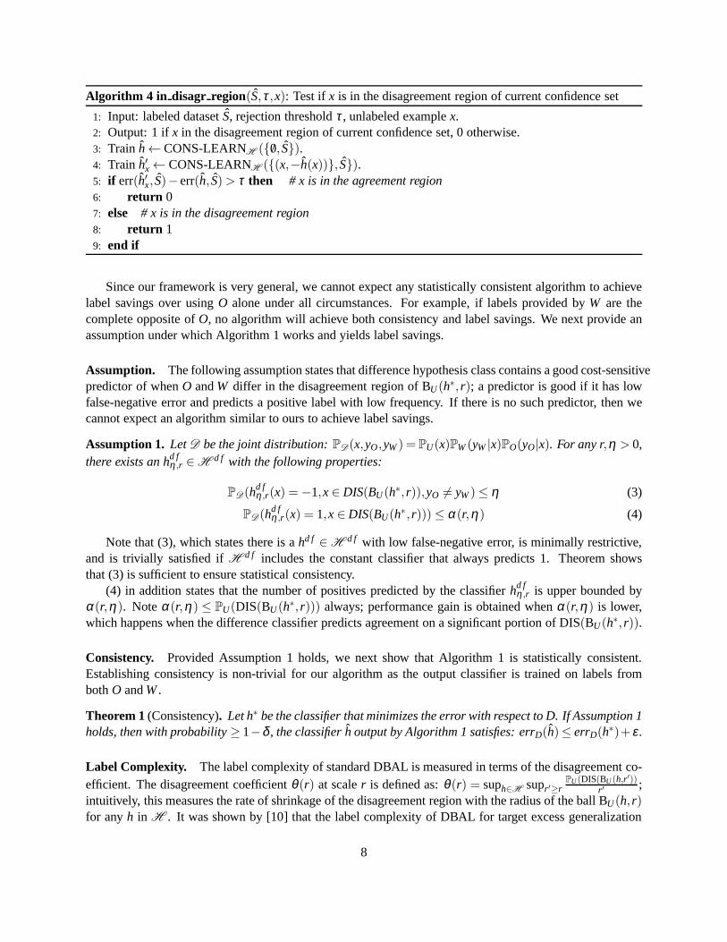
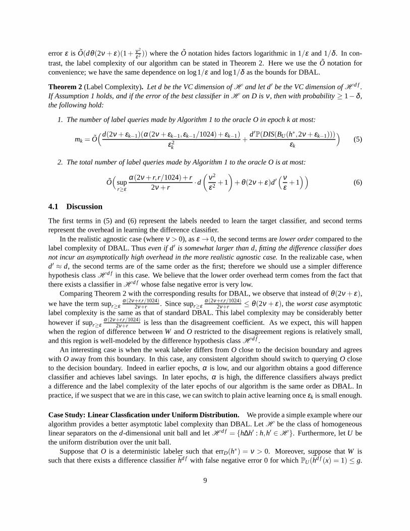
Case Study: Linear Classfication under Uniform Distribution. We provide a simple example where ouralgorithm provides a better asymptotic label complexity than DBAL. LetH be the class of homogeneouslinear separators on thed-dimensional unit ball and letH d f = {h∆h′ : h,h′ ∈H }. Furthermore, letU bethe uniform distribution over the unit ball.
Suppose thatO is a deterministic labeler such that errD(h∗) = ν > 0. Moreover, suppose thatW issuch that there exists a difference classifierhd f with false negative error 0 for whichPU(hd f (x) = 1) ≤ g.
9
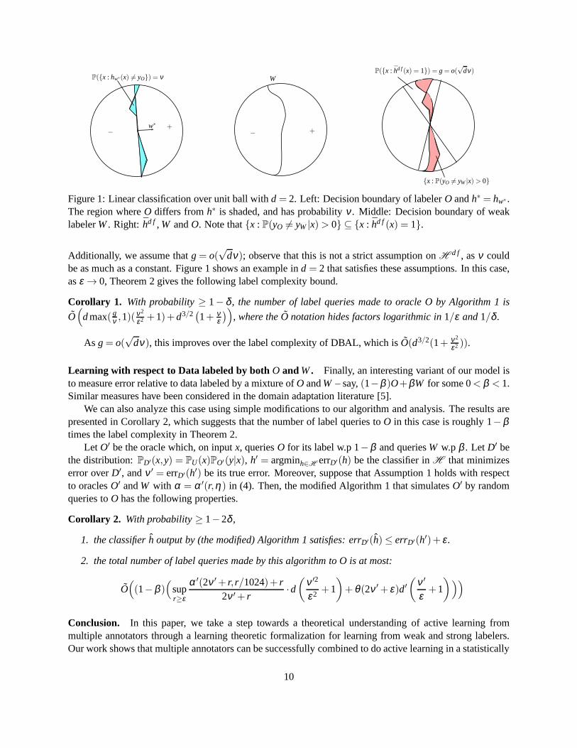
+−
w∗
P({x : hw∗(x) 6= yO}) = ν
+−
W
{x : P(yO 6= yW|x)> 0}
P({x : hd f(x) = 1}) = g= o(√
dν)
Figure 1: Linear classification over unit ball withd = 2. Left: Decision boundary of labelerO andh∗ = hw∗ .The region whereO differs fromh∗ is shaded, and has probabilityν . Middle: Decision boundary of weaklabelerW. Right: hd f , W andO. Note that{x : P(yO 6= yW|x)> 0} ⊆ {x : hd f (x) = 1}.
Additionally, we assume thatg= o(√
dν); observe that this is not a strict assumption onH d f , asν couldbe as much as a constant. Figure 1 shows an example ind = 2 that satisfies these assumptions. In this case,asε → 0, Theorem 2 gives the following label complexity bound.
Corollary 1. With probability≥ 1− δ , the number of label queries made to oracle O by Algorithm 1 is
O(
dmax( gν ,1)(
ν2
ε2 +1)+d3/2(
1+ νε)
)
, where theO notation hides factors logarithmic in1/ε and1/δ .
As g= o(√
dν), this improves over the label complexity of DBAL, which isO(d3/2(1+ ν2
ε2 )).
Learning with respect to Data labeled by bothO andW. Finally, an interesting variant of our model isto measure error relative to data labeled by a mixture ofO andW – say,(1−β )O+βW for some 0< β < 1.Similar measures have been considered in the domain adaptation literature [5].
We can also analyze this case using simple modifications to our algorithm and analysis. The results arepresented in Corollary 2, which suggests that the number of label queries toO in this case is roughly 1−βtimes the label complexity in Theorem 2.
Let O′ be the oracle which, on inputx, queriesO for its label w.p 1−β and queriesW w.p β . Let D′ bethe distribution:PD′(x,y) = PU(x)PO′(y|x), h′ = argminh∈H errD′(h) be the classifier inH that minimizeserror overD′, andν ′ = errD′(h′) be its true error. Moreover, suppose that Assumption 1 holdswith respectto oraclesO′ andW with α = α ′(r,η) in (4). Then, the modified Algorithm 1 that simulatesO′ by randomqueries toO has the following properties.
Corollary 2. With probability≥ 1−2δ ,
1. the classifierh output by (the modified) Algorithm 1 satisfies: errD′(h)≤ errD′(h′)+ ε .
2. the total number of label queries made by this algorithm toO is at most:
O(
(1−β )(
supr≥ε
α ′(2ν ′+ r, r/1024)+ r2ν ′+ r
·d(
ν ′2
ε2 +1
)
+θ(2ν ′+ ε)d′(
ν ′
ε+1
)
))
Conclusion. In this paper, we take a step towards a theoretical understanding of active learning frommultiple annotators through a learning theoretic formalization for learning from weak and strong labelers.Our work shows that multiple annotators can be successfullycombined to do active learning in a statistically
10
consistent manner under a general setting with few assumptions; moreover, under reasonable conditions, thiskind of learning can provide label savings over plain activelearning.
An avenue for future work is to explore a more general settingwhere we have multiple labelers withexpertise on different regions of the input space. Can we combine inputs from such labelers in a statisticallyconsistent manner? Second, our algorithm is intended for a setting whereW is biased, and performs sub-optimally when the label generated byW is a random corruption of the label provided byO. How can weaccount for both random noise and bias in active learning from weak and strong labelers?
Acknowledgements
We thank NSF under IIS 1162581 for research support and Jennifer Dy for introducing us to the problem ofactive learning from multiple labelers.
References
[1] M.-F. Balcan, A. Beygelzimer, and J. Langford. Agnosticactive learning. J. Comput. Syst. Sci.,75(1):78–89, 2009.
[2] M.-F. Balcan and P. M. Long. Active and passive learning of linear separators under log-concavedistributions. InCOLT, 2013.
[3] A. Beygelzimer, D. Hsu, J. Langford, and T. Zhang. Activelearning with an ERM oracle, 2009.
[4] A. Beygelzimer, D. Hsu, J. Langford, and T. Zhang. Agnostic active learning without constraints. InNIPS, 2010.
[5] J. Blitzer, K. Crammer, A. Kulesza, F. Pereira, and J. Wortman. Learning bounds for domain adapta-tion. In NIPS, pages 129–136, 2007.
[6] Nader H. Bshouty and Lynn Burroughs. Maximizing agreements with one-sided error with applicationsto heuristic learning.Machine Learning, 59(1-2):99–123, 2005.
[7] D. A. Cohn, L. E. Atlas, and R. E. Ladner. Improving generalization with active learning.MachineLearning, 15(2), 1994.
[8] K. Crammer, M. J. Kearns, and J. Wortman. Learning from data of variable quality. InNIPS, pages219–226, 2005.
[9] S. Dasgupta. Coarse sample complexity bounds for activelearning. InNIPS, 2005.
[10] S. Dasgupta, D. Hsu, and C. Monteleoni. A general agnostic active learning algorithm. InNIPS, 2007.
[11] O. Dekel, C. Gentile, and K. Sridharan. Selective sampling and active learning from single and multipleteachers.JMLR, 13:2655–2697, 2012.
[12] P. Donmez and J. Carbonell. Proactive learning: Cost-sensitive active learning with multiple imperfectoracles. InCIKM, 2008.
11
[13] Meng Fang, Xingquan Zhu, Bin Li, Wei Ding, and Xindong Wu. Self-taught active learning fromcrowds. InData Mining (ICDM), 2012 IEEE 12th International Conference on, pages 858–863. IEEE,2012.
[14] S. Hanneke. A bound on the label complexity of agnostic active learning. InICML, 2007.
[15] D. Hsu. Algorithms for Active Learning. PhD thesis, UC San Diego, 2010.
[16] Panagiotis G Ipeirotis, Foster Provost, Victor S Sheng, and Jing Wang. Repeated labeling using multi-ple noisy labelers.Data Mining and Knowledge Discovery, 28(2):402–441, 2014.
[17] Adam Tauman Kalai, Varun Kanade, and Yishay Mansour. Reliable agnostic learning.J. Comput.Syst. Sci., 78(5):1481–1495, 2012.
[18] Varun Kanade and Justin Thaler. Distribution-independent reliable learning. InProceedings of The27th Conference on Learning Theory, COLT 2014, Barcelona, Spain, June 13-15, 2014, pages 3–24,2014.
[19] C.H. Lin, Mausam, and D.S. Weld. Reactive learning: Actively trading off larger noisier training setsagainst smaller cleaner ones. InICML Workshop on Crowdsourcing and Machine Learning and ICMLActive Learning Workshop, 2015.
[20] Christopher H. Lin, Mausam, and Daniel S. Weld. To re(label), or not to re(label). InProceedings ofthe Seconf AAAI Conference on Human Computation and Crowdsourcing, HCOMP 2014, November2-4, 2014, Pittsburgh, Pennsylvania, USA, 2014.
[21] L. Malago, N. Cesa-Bianchi, and J. Renders. Online active learning with strong and weak annotators.In NIPS Workshop on Learning from the Wisdom of Crowds, 2014.
[22] R. D. Nowak. The geometry of generalized binary search.IEEE Transactions on Information Theory,57(12):7893–7906, 2011.
[23] Hans Ulrich Simon. Pac-learning in the presence of one-sided classification noise.Ann. Math. Artif.Intell., 71(4):283–300, 2014.
[24] S. Song, K. Chaudhuri, and A. D. Sarwate. Learning from data with heterogeneous noise using sgd.In AISTATS, 2015.
[25] R. Urner, S. Ben-David, and O. Shamir. Learning from weak teachers. InAISTATS, pages 1252–1260,2012.
[26] S. Vijayanarasimhan and K. Grauman. What’s it going to cost you?: Predicting effort vs. informative-ness for multi-label image annotations. InCVPR, pages 2262–2269, 2009.
[27] S. Vijayanarasimhan and K. Grauman. Cost-sensitive active visual category learning.IJCV, 91(1):24–44, 2011.
[28] P. Welinder, S. Branson, S. Belongie, and P. Perona. Themultidimensional wisdom of crowds. InNIPS, pages 2424–2432, 2010.
[29] Y. Yan, R. Rosales, G. Fung, and J. G. Dy. Active learningfrom crowds. InICML, pages 1161–1168,2011.
12
[30] Y. Yan, R. Rosales, G. Fung, F. Farooq, B. Rao, and J. G. Dy. Active learning from multiple knowledgesources. InAISTATS, pages 1350–1357, 2012.
[31] C. Zhang and K. Chaudhuri. Beyond disagreement-based agnostic active learning. InNIPS, 2014.
13
A Notation
A.1 Basic Definitions and Notation
Here we do a brief recap of notation. We assume that we are given a target hypothesis classH of VCdimensiond, and a difference hypothesis classH d f of VC dimensiond′.
We are given access to an unlabeled distributionU and two labeling oraclesO andW. QueryingO (resp.W) with an unlabeled data pointxi generates a labelyi,O (resp. yi,W) which is drawn from the distributionPO(y|xi) (resp.PW(y|xi)). In general these two distributions are different. We use the notationD to denotethe joint distribution over examples and labels fromO andW:
PD(x,yO,yW) = PU(x)PO(yO|x)PW(yW|x)
Our goal in this paper is to learn a classifier inH which has low error with respect to the data distributionD described as:PD(x,y) = PU(x)PO(y|x) and our goal is use queries toW to reduce the number of queriesto O. We useyO to denote the labels returned byO, yW to denote the labels returned byW.
The error of a classifierh under a labeled data distributionQ is defined as: errQ(h) = P(x,y)∼Q(h(x) 6= y);we use the notation err(h,S) to denote its empirical error on a labeled data setS. We use the notationh∗ todenote the classifier with the lowest error underD. Define the excess error ofh with respect to distributionD as errD(h)−errD(h∗). For a setZ, we occasionally abuse notation and useZ to also denote the uniformdistribution over the elements ofZ.
Confidence Sets and Disagreement Region.Our active learning algorithm will maintain a(1− δ )-confidence setfor h∗ throughout the algorithm. A set of classifiersV ⊆H produced by a (possibly ran-domized) algorithm is said to be a(1− δ )-confidence set forh∗ if h∗ ∈ V with probability≥ 1− δ ; herethe probability is over the randomness of the algorithm as well as the choice of all labeled and unlabeledexamples drawn by it.
Given two classifiersh1 andh2 the disagreement betweenh1 andh2 under an unlabeled data distributionU , denoted byρU(h1,h2), isPx∼U(h1(x) 6= h2(x)). Given an unlabeled datasetS, the empirical disagreementof h1 andh2 on S is denoted byρS(h1,h2). Observe that the disagreements underU form a pseudometricoverH . We use BU(h, r) to denote a ball of radiusr centered aroundh in this metric. Thedisagreementregion of a setV of classifiers, denoted by DIS(V), is the set of all examplesx ∈X such that there existtwo classifiersh1 andh2 in V for which h1(x) 6= h2(x).
Disagreement Region. We denote the disagreement region of a disagreement ball of radiusr centeredaroundh∗ by
∆(r) := DIS(B(h∗, r)) (7)
Concentration Inequalities. SupposeZ is a dataset consisting ofn iid samples from a distributionD. Wewill use the following result, which is obtained from a standard application of the normalized VC inequality.With probability 1−δ over the random draw ofZ, for all h,h′ ∈H ,
|(err(h,Z)−err(h′,Z))− (errD(h)−errD(h′))|
≤ min(√
σ(n,δ )ρZ(h,h′)+σ(n,δ ),√
σ(n,δ )ρD(h,h′)+σ(n,δ ))
(8)
|(err(h,Z)−errD(h)|≤ min
(√
σ(n,δ )err(h,Z)+σ(n,δ ),√
σ(n,δ )errD(h)+σ(n,δ ))
(9)
14
whered is the VC dimension ofH and the notationσ(n,δ ) is defined as:
σ(n,δ ) =8n(2d ln
2end
+ ln24δ) (10)
Equation (8) loosely implies the following equation:
|(err(h,Z)−err(h′,Z))− (errD(h)−errD(h′))| ≤
√
4σ(n,δ ) (11)
The following is a consequence of standard Chernoff bounds.Let X1, . . . ,Xn be iid Bernoulli random vari-ables with meanp. If p= ∑i Xi/n, then with probabiliy 1−δ ,
|p− p| ≤min(√
pγ(n,δ )+ γ(n,δ ),√
pγ(n,δ )+ γ(n,δ )) (12)
where the notationγ(n,δ ) is defined as:
γ(n,δ ) =4n
ln2δ
(13)
Equation (12) loosely implies the following equation:
|p− p| ≤√
4γ(n,δ ) (14)
Using the notation we just introduced, we can rephrase Assumption 1 as follows. For anyr,η > 0, thereexists anhd f
η ,r ∈H d f with the following properties:
PD(hd fη ,r(x) =−1,x∈ ∆(r),yO 6= yW)≤ η
PD(hd fη ,r(x) = 1,x∈ ∆(r))≤ α(r,η)
We end with an useful fact aboutσ(n,δ ).
Fact 1. The minimum n such thatσ(n,δ/(logn(logn+1)))≤ ε is at most
64ε(d ln
512ε
+ ln24δ)
A.2 Adaptive Procedure for Estimating Probability Mass
For completeness, we describe in Algorithm 5 a standard doubling procedure for estimating the bias of acoin within a constant factor. This procedure is used by Algorithm 2 to estimate the probability mass of thedisagreement region of the current confidence set based on unlabeled examples drawn fromU .
Lemma 1. Suppose p> 0 and Algorithm 5 is run with failure probabilityδ . Then with probability1− δ ,(1) the outputp is such thatp≤ p≤ 2p. (2) The total number of calls toO is at most O( 1
p2 ln 1δ p).
Proof. Consider the event
E = { for all i ∈ N, |pi− p| ≤
√
4ln 2·2i
δ2i }
15
Algorithm 5 Adaptive Procedure for Estimating the Bias of a Coin1: Input: failure probabilityδ , an oracleO which returns iid Bernoulli random variables with unknown
biasp.2: Output: p, an estimate of biasp such that ˆp≤ p≤ 2p with probability≥ 1−δ .3: for i = 1,2, . . . do4: Call the oracleO 2i times to get empirical frequency ˆpi .
5: if
√
4ln 4·2iδ
2i ≤ pi/3 then return p= 2pi3
6: end if7: end for
By Equation (14) and union bound,P(E)≥ 1−δ . On eventE, we claim that ifi is large enough that
4
√
4ln 4·2i
δ2i ≤ p (15)
then the condition in line 5 will be met. Indeed, this implies
√
4ln 4·2i
δ2i ≤
p−√
4ln 4·2iδ
2i
3≤ pi
3
Definei0 as the smallest numberi such that Equation (15) is true. Then by algebra, 2i0 =O( 1p2 ln 1
δ p). Hence
the number of calls to oracleO is at most 1+2+ . . .+2i0 = O( 1p2 ln 1
δ p).Consider the smallesti∗ such that the condition in line 5 is met. We have that
√
4ln 4·2i∗
δ2i∗ ≤ pi∗/3
By the definition ofE,|p− pi∗ | ≤ pi∗/3
that is, 2pi∗/3≤ p≤ 4pi∗/3, implying p≤ p≤ 2p.
A.3 Notations on Datasets
Without loss of generality, assume the examples drawn throughout Algorithm 1 have distinct feature valuesx, since this happens with probability 1 under mild assumptions.
Algorithm 1 uses a mixture of three kinds of labeled data to learn a target classifier – labels obtainedfrom queryingO, labels inferred by the algorithm, and labels obtained fromqueryingW. To analyze theeffect of these three kinds of labeled data, we need to introduce some notation.
Recall that we define the joint distributionD over examples and labels both fromO andW as follows:
PD(x,yO,yW) = PU(x)PO(yO|x)PW(yW|x)
where given an examplex, the labels generated byO andW are conditionally independent.
16
A datasetSwith empirical error minimizerh and a rejection thresholdτ define a implicit confidence setfor h∗ as follows:
V(S,τ) = {h : err(h, S)−err(h, S)≤ τ}At the beginning of epochk, we haveSk−1. hk−1 is defined as the empirical error minimizer ofSk−1. The dis-agreement region of the implicit confidence set at epochk, Rk−1 is defined asRk−1 := DIS(V(Sk−1,3εk/2)).Algorithm 4 in disagr region(Sk−1,3εk/2,x) provides a test deciding if an unlabeled examplex is insideRk−1 in epochk. (See Lemma 6.)
DefineAk to be the distributionD conditioned on the set{(x,yO,yW) : x ∈ Rk−1}. At epochk, Algo-rithm 2 has inputs distributionU , oraclesW andO, target false negative errorε = εk/128, hypothesis classH d f , confidenceδ = δk/2, previous labeled datasetSk−1, and outputs a difference classfierhd f
k . By thesetting ofm in Equation (1), Algorithm 2 first computes ˆpk using unlabeled examples drawn fromU , whichis an estimator ofPD (x∈ Rk−1). Then it draws a subsample of size
mk,1 =64·1024pk
εk(d ln
512·1024pk
εk+ ln
144δk
) (16)
iid from Ak. We call the resulting datasetA ′k .
At epochk, Algorithm 3 performs adaptive subsampling to refine the implicit (1− δ )-confidence set.For each roundt, it subsamplesU to get an unlabeled datasetSt,U
k of size 2t . Define the corresponding(hypothetical) dataset with labels queried from bothW andO asS t
k . Stk, the (hypothetical) dataset with
labels queried fromO, is defined as:
Stk = {(x,yO)|(x,yO,yW) ∈S
tk}
In addition to obtaining labels fromO, the algorithm obtains labels in two other ways. First, if anx ∈X \Rk−1, then its label is safely inferred and with high probability, this inferred labelhk−1(x) is equal toh∗(x). Second, if anx lies in Rk−1 but if the difference classifierhd f
k predicts agreement betweenO andW,then its label is obtained by queryingW. The actual datasetSt
k generated by Algorithm 3 is defined as:
Stk = {(x, hk−1(x))|(x,yO,yW) ∈S
tk ,x /∈ Rk−1}∪{(x,yO)|(x,yO,yW) ∈S
tk ,x∈ Rk−1, h
d fk (x) = +1}
∪{(x,yW)|(x,yO,yW) ∈Stk ,x∈ Rk−1, h
d fk (x) =−1}
We useDk to denote the labeled data distribution as follows:
PDk(x,y) = PU(x)PQk
(y|x)
PQk(y|x) =
I(hk−1(x) = y), x /∈Rk−1
PO(y|x), x∈Rk−1, hd fk (x) = +1
PW(y|x), x∈Rk−1, hd fk (x) =−1
Therefore,Stk can be seen as a sample of size 2t drawn iid fromDk.
Observe thathtk is obtained by training an ERM classifier overSt
k, andδ tk = δk/2t(t +1).
Suppose Algorithm 3 stops at iterationt0(k), then the final dataset returned isSk = St0(k)k , with a total
number ofmk,2 label requests toO. We defineSk = St0(k)k , Sk = S
t0(k)k andσk = σ(2t0(k),δ t0(k)
k ).
17
Fork= 0, we define the notationSk differently. S0 is the dataset drawn iid at random fromD, with labelsqueried entirely toO. For notational convenience, defineS0 = S0. σ0 is defined asσ0 = σ(n0,δ0), whereσ(·, ·) is defined by Equation (10) andn0 is defined as:
n0 = (64·10242)(2d ln(512·10242)+ ln96δ)
Recall thathk = argminh∈H err(h, Sk) is the empirical error minimizer with respect to the datasetSk.Note that the empirical distanceρZ(·, ·) does not depend on the labels in datasetZ, therefore,ρSk
(h,h′) =ρSk(h,h
′). We will use them interchangably throughout.
Table 1: Summary of Notations.
Notation Explanation Samples Drawn from
D Joint distribution of(x,yW,yO) -D Joint distribution of(x,yO) -U Marginal distribution ofx -O Conditional distribution ofyO givenx -W Conditional distribution ofyW givenx -
Rk−1 Disagreement region at epochk -Ak Conditional distribution of(x,yW,yO) givenx∈ Rk−1 -A ′
k Dataset used to train difference classifier at epochk Ak
hd fk Difference classifierhd f
2ν+εk−1,εk/512, wherehη ,r is defined in Assump-tion 1
-
hd fk Difference classifier returned by Algorithm 2 at epochk -
St,Uk unlabeled dataset drawn at iterationt of Algorithm 3 at epochk≥ 1 U
S tk St,U
k augmented by labels fromO andW D
Stk {(x,yO)|(x,yO,yW) ∈S t
k} DSt
k Labeled dataset produced at iterationt of Algorithm 3 at epochk≥ 1 Dk
Dk Distribution of Stk for k≥ 1 and anyt. Has marginalU over X . The
conditional distribution ofy|x is I(h∗(x)) if x /∈ Rk−1, W if x∈ Rk−1 andhd f (x) =−1, andO otherwise
-
t0(k) Number of iterations of Algorithm 3 at epochk≥ 1 -
S0 Initial dataset drawn by Algorithm 1 D
Sk Dataset finally returned by Algorithm 3 at epochk≥ 1. Equal toSt0(k)k Dk
Sk Dataset obtained by replacing all labels inSk by labels drawn fromO.Equal toSt0(k)
k
D
Sk Equal toSt0(k)k D
hk Empirical error minimizer onSk -
18
A.4 Events
Recall thatδk = δ/(4(k+1)2),εk = 2−k.Define
hd fk = hd f
2ν+εk−1,εk/512
where the notationhd fr,η is introduced in Assumption 1.
We begin by defining some events that we will condition on later in the proof, and showing that theseevents occur with high probability.
Define event
E1k :=
{
PD(x∈ Rk−1)/2≤ pk ≤ PD (x∈Rk−1),
and For allhd f ∈Hd f ,
|PA ′k(hd f (x) =−1,yO 6= yW)−PAk(h
d f (x) =−1,yO 6= yW)| ≤ εk
1024PD (x∈Rk−1)
+
√
min(PAk(hd f (x) =−1,yO 6= yW),PA ′
k(hd f (x) =−1,yO 6= yW))
εk
1024PD (x∈ Rk−1)
and|PA ′k(hd f (x) = +1)−PAk(h
d f (x) = +1)|
≤√
min(PAk(hd f (x) = +1),PA ′
k(hd f (x) = +1))
εk
1024PD (x∈Rk−1)+
εk
1024PD (x∈ Rk−1)
}
Fact 2. P(E1k)≥ 1−δk/2.
Define event
E2k =
{
For all t ∈ N, for all h,h′ ∈H ,
|(err(h,Stk)−err(h′,St
k))− (errD(h)−errD(h′))| ≤ σ(2t ,δ t
k)+√
σ(2t ,δ tk)ρSt
k(h,h′)
and err(h, Stk)−errDk
(h) ≤ σ(2t ,δ tk)+
√
σ(2t ,δ tk)errDk
(h)
and PS tk(hd f
k (x) =−1,yO 6= yW,x∈Rk−1)−PD(hd fk (x) =−1,yO 6= yW,x∈ Rk−1)
≤√
γ(2t ,δ tk)PS t
k(hd f
k (x) =−1,yO 6= yW,x∈Rk−1)+ γ(2t ,δ tk)
and PS tk(hd f
k (x) =−1∩x∈Rk−1)≤ 2(PD (hd fk (x) =−1,x∈ Rk−1)+ γ(2t ,δ t
k))}
Fact 3. P(E2k)≥ 1−δk/2.
We will also use the following definitions of events in our proof. Define eventF0 as
F0={
for all h,h′ ∈H , |(err(h,S0)−err(h′,S0))−(errD(h)−errD(h′))| ≤σ(n0,δ0)+
√
σ(n0,δ0)ρS0(h,h′)}
For k∈ {1,2, . . . ,k0}, eventFk is defined inductively as
Fk = Fk−1∩ (E1k ∩E2
k)
Fact 4. For k∈ {0,1, . . . ,k0}, P(Fk)≥ 1−δ0−δ1− . . .−δk. Specifically,P(Fk0)≥ 1−δ .
The proofs of Facts 2, 3 and 4 are provided in Appendix E.
19
B Proof Outline and Main Lemmas
The main idea of the proof is to maintain the following three invariants on the outputs of Algorithm 1 ineach epoch. We prove that these invariants hold simultaneously for each epoch with high probability byinduction over the epochs. Throughout, fork≥ 1, the end of epochk refers to the end of execution of line13 of Algorithm 1 at iterationk. The end of epoch 0 refers to the end of execution of line 5 in Algorithm 1.
Invariant 1 states that if we replace the inferred labels andlabels obtained fromW in Sk by those obtainedfrom O (thus getting the datasetSk), then the excess errors of classifiers inH will not decrease by much.
Invariant 1 (Approximate Favorable Bias). Let h be any classifier inH , and h′ be another classifier inHwith excess error on D no greater thanεk. Then, at the end of epoch k, we have:
err(h,Sk)−err(h′,Sk)≤ err(h, Sk)−err(h′, Sk)+ εk/16
Invariant 2 establishes that in epochk, Algorithm 3 selects enough examples so as to ensure that con-centration of empirical errors of classifiers inH on Sk to their true errors.
Invariant 2 (Concentration). At the end of epoch k,Sk, Sk andσk are such that:1. For any pair of classifiers h,h′ ∈H , it holds that:
|(err(h,Sk)−err(h′,Sk))− (errD(h)−errD(h′))| ≤ σk+
√
σkρSk(h,h′) (17)
2. The datasetSk has the following property:
σk+
√
σkerr(hk, Sk)≤ εk/512 (18)
Finally, Invariant 3 ensures that the difference classifierproduced in epochk has low false negative erroron the disagreement region of the(1−δ ) confidence set at epochk.
Invariant 3 (Difference Classifier). At epoch k, the difference classifier output by Algorithm 2 issuch that
PD(hd fk (x) =−1,yO 6= yW,x∈ Rk−1)≤ εk/64 (19)
PD(hd fk (x) = +1,x∈ Rk−1)≤ 6(α(2ν + εk−1,εk/512)+ εk/1024) (20)
We will show the following property about the three invariants. Its proof is deferred to Subsection B.4.
Lemma 2. There is a numerical constant c0 > 0 such that the following holds. The collection of events{Fk}k0
k=0 is such that for k∈ {0,1, . . . ,k0}:(1) If k= 0, then on event Fk, at epoch k,
(1.1) Invariants 1,2 hold.(1.2) The number of label requests to O is at most m0≤ c0(d+ ln 1
δ ).(2) If k≥ 1, then on event Fk, at epoch k,
(2.1) Invariants 1,2,3 hold.(2.2) the number of label requests to O is at most
mk≤ c0
((α(2ν + εk−1,εk/1024)+ εk)(ν + εk)
ε2k
d(ln2 1εk
+ ln2 1δk)+
PU(x∈ ∆(2ν + εk−1))
εk(d′ ln
1εk
+ ln1δk))
20
B.1 Active Label Inference and Identifying the Disagreement Region
We begin by proving some lemmas about Algorithm 4 which identifies if an example lies in the disagreementregion of the current confidence set. This is done by using a constrained ERM oracle CONS-LEARNH(·, ·)using ideas similar to [10, 15, 3, 4].
Lemma 3. When given as input a datasetS, a thresholdτ > 0, an unlabeled example x, Algorithm 4in disagr region returns 1 if and only if x lies inside DIS(V(S,τ)).
Proof. (⇒) If Algorithm 4 returns 1, then we have found a classifierh′x such that (1)hx(x) =−h(x), and (2)err(h′x, S)−err(h, S)≤ τ , i.e. h′x ∈V(S,τ). Therefore,x is in DIS(V(S,τ)).(⇐) If x is in DIS(V(S,τ)), then there exists a classifierh∈H such that (1)h(x) =−h(x) and (2) err(h, S)−err(h, S)≤ τ . Hence by definition ofh′x, err(h′x, S)−err(h, S)≤ τ . Thus, Algorithm 4 returns 1.
We now provide some lemmas about the behavior of Algorithm 4 called at epochk.
Lemma 4. Suppose Invariants 1 and 2 hold at the end of epoch k− 1. If h ∈H is such that errD(h) ≤errD(h∗)+ εk−1/2, then
err(h, Sk−1)−err(hk−1, Sk−1)≤ 3εk−1/4
Proof. If h∈H has excess error at mostεk−1/2 with respect toD, then,
err(h, Sk−1)−err(hk−1, Sk−1)
≤ err(h,Sk−1)−err(hk−1,Sk−1)+ εk−1/16
≤ errD(h)−errD(hk−1)+σk−1+
√
σk−1ρSk−1(h, hk−1)+ εk−1/16
≤ εk−1/2+σk−1+
√
σk−1ρSk−1(h, hk−1)+ εk−1/16
≤ 9εk−1/16+σk−1+
√
σk−1err(h, Sk−1)+
√
σk−1err(hk−1, Sk−1)
≤ 9εk−1/16+σk−1+
√
σk−1err(h, Sk−1)+
√
σk−1(err(hk−1, Sk−1)+9εk−1/16)
Where the first inequality follows from Invariant 1, the second inequality from Equation (17) of Invariant 2,the third inequality from the assumption thathhas excess error at mostεk−1/2, and the fourth inequality fromthe triangle inequality, the fifth inequality is by adding a nonnegative number in the last term. Continuing,
err(h, Sk−1)−err(hk−1, Sk−1)
≤ 9εk−1/16+4σk−1+2√
σk−1(err(hk−1, Sk−1)+9εk−1/16)
≤ 9εk−1/16+4σk−1+2√
σk−1err(hk−1, Sk−1)+2√
εk−1/512·9εk−1/16
≤ 9εk−1/16+ εk−1/32+2√
εk−1/512·9εk−1/16
≤ 3εk−1/4
Where the first inequality is by simple algebra (by lettingD = err(h, Sk−1), E = err(hk−1, Sk−1)+9εk−1/16,F = σk−1 in D≤ E+F +
√DF +
√EF⇒ D≤ E+4F +2
√EF), the second inequality is from
√A+B≤√
A+√
B andσk−1≤ εk−1/512 which utilizes Equation (18) of Invariant 2, the third inequality is again byEquation (18) of Invariant 2, the fourth inequality is by algebra.
21
Lemma 5. Suppose Invariants 1 and 2 hold at the end of epoch k−1. Then,
errD(hk−1)−errD(h∗)≤ εk−1/8
Proof. By Lemma 4, we know that sinceh∗ has excess error 0 with respect toD,
err(h∗, Sk−1)−err(hk−1, Sk−1)≤ 3εk−1/4 (21)
Therefore,
errD(hk−1)−errD(h∗)
≤ err(hk−1,Sk−1)−err(h∗,Sk−1)+σk−1+√
σk−1ρSk−1(hk−1,h∗)
≤ err(hk−1, Sk−1)−err(h∗, Sk−1)+σk−1+
√
σk−1ρSk−1(hk−1,h∗)+ εk−1/16
≤ εk−1/16+σk−1+
√
σk−1(err(hk−1, Sk−1)+err(h∗, Sk−1))
≤ εk−1/16+σk−1+
√
σk−1(2err(hk−1, Sk−1)+3εk−1/4)
≤ εk−1/16+σk−1+
√
2σk−1err(hk−1, Sk−1)+√
εk−1/512·3εk−1/4
≤ εk−1/8
where the first inequality is from Equation (17) of Invariant2, the second inequality uses Invariant 1, thethird inequality follows from the optimality ofhk−1 and triangle inequality, the fourth inequality uses Equa-tion (21), the fifth inequality uses the fact that
√A+B≤
√A+√
B andσk−1 ≤ εk−1/512, which is fromEquation (18) of Invariant 2, the last inequality again utilizes the Equation (18) of Invariant 2.
Lemma 6. Suppose Invariants 1, 2, and 3 hold in epoch k−1 conditioned on event Fk−1. Then conditionedon event Fk−1, the implicit confidence set Vk−1 =V(Sk−1,3εk/2) is such that:(1) If h∈H satisfies errD(h)−errD(h∗)≤ εk, then h is in Vk−1.(2) If h∈H is in Vk−1, then errD(h)−errD(h∗)≤ εk−1. Hence Vk−1⊆ BU(h∗,2ν + εk−1).(3) Algorithm 4,in disagr region, when run on inputs datasetSk−1, threshold3εk/2, unlabeled example x,returns 1 if and only if x is in Rk−1.
Proof. (1) Let h be a classifier with errD(h)− errD(h∗) ≤ εk = εk−1/2. Then, by Lemma 4, one haserr(h, Sk−1)−err(hk−1, Sk−1)≤ 3εk−1/4= 3εk/2. Hence,h is inVk−1.(2) Fix anyh in Vk−1, by definition ofVk−1,
err(h, Sk−1)−err(hk−1, Sk−1)≤ 3εk/2= 3εk−1/4 (22)
Recall that from Lemma 5,errD(hk−1)−errD(h
∗)≤ εk−1/8
Thus for classifierh, applying Invariant 1 by takingh′ := hk−1, we get
err(h,Sk−1)−err(hk−1,Sk−1)≤ err(h, Sk−1)−err(hk−1, Sk−1)+ εk−1/32 (23)
22
Therefore,
errD(h)−errD(hk−1)
≤ err(h,Sk−1)−err(hk−1,Sk−1)+σk−1+√
σk−1ρSk−1(h, hk−1)
≤ err(h,Sk−1)−err(hk−1,Sk−1)+σk−1+
√
σk−1(err(h, Sk−1)+err(hk−1, Sk−1))
≤ err(h, Sk−1)−err(hk−1, Sk−1)+σk−1+
√
σk−1(err(h, Sk−1)+err(hk−1, Sk−1))+ εk−1/16
≤ 13εk−1/16+σk−1+
√
σk−1(2err(hk−1, Sk−1)+3εk−1/4)
≤ 13εk−1/16+σk−1+
√
2σk−1err(hk−1, Sk−1)+√
εk−1/512·3εk−1/4
≤ 7εk−1/8
where the first inequality is from Equation (17) of Invariant2, the second inequality uses the fact thatρSk−1
(h,h′) = ρSk−1(h,h′)≤ err(h, Sk−1)+err(h′, Sk−1) for h,h′ ∈H , the third inequality uses Equation (23);
the fourth inequality is from Equation (22); the fifth inequality is from the fact that√
A+B≤√
A+√
Bandσk−1 ≤ εk−1/512, which is from Equation (18) of Invariant 2, the last inequality again follows fromEquation (18) of Invariant 2 and algebra.In conjunction with the fact that errD(hk−1)−errD(h∗)≤ εk−1/8, this implies
errD(h)−errD(h∗)≤ εk−1
By triangle inequality,ρ(h,h∗)≤ 2ν + εk−1, henceh∈ BU(h∗,2ν + εk−1). In summaryVk−1⊆ BU(h∗,2ν +εk−1).(3) Follows directly from Lemma 3 and the fact thatRk−1 = DIS(Vk−1).
B.2 Training the Difference Classifier
Recall that∆(r) = DIS(BU(h∗, r)) is the disagreement region of the disagreement ball centered aroundh∗
with radiusr.
Lemma 7 (Difference Classifier Invariant). There is a numerical constant c1 > 0 such that the followingholds. Suppose that Invariants 1 and 2 hold at the end of epochk− 1 conditioned on event Fk−1 andthat Algorithm 2 has inputs unlabeled data distribution U, oracle O, ε = εk/128, hypothesis classH d f ,δ = δk/2, previous labeled datasetSk−1. Then conditioned on event Fk,(1) hd f
k , the output of Algorithm 2, maintains Invariant 3.(2)(Label Complexity: Part 1.) The number of label queries made to O is at most
mk,1≤ c1
(
PU(x∈ ∆(2ν + εk−1))
εk(d′ ln
1εk
+ ln1δk))
Proof. (1) Recall thatFk = Fk−1∩E1k ∩E2
k , whereE1k , E2
k are defined in Subsection A.4. Suppose eventFk
happens.
23
Proof of Equation (19). Recall thathd fk is the optimal solution of optimization problem (2). We haveby
feasibility and the fact that on eventE3k , 2pk ≥ PD(x∈ Rk−1),
PA ′k(hd f
k (x) =−1,yO 6= yW)≤ εk
256pk≤ εk
128PD (x∈ Rk−1)
By definition of eventE2k , this implies
PAk(hd fk (x) =−1,yO 6= yW)
≤ PA ′k(hd f
k (x) =−1,yO 6= yW)+
√
PA ′k(hd f
k (x) =−1,yO 6= yW)εk
1024PD (x∈ Rk−1)+
εk
1024PD (x∈ Rk−1)
≤ εk
64PD (x∈ Rk−1)
Indicating
PD(hd fk (x) =−1,yO 6= yW,x∈ Rk−1)≤
εk
64
Proof of Equation (20). By definition ofhd fk in Subsection A.4,hd f
k is such that:
PD (hd fk (x) = +1,x∈ ∆(2ν + εk−1))≤ α(2ν + εk−1,εk/512)
PD(hd fk (x) =−1,yO 6= yW,x∈ ∆(2ν + εk−1))≤ εk/512
By item (2) of Lemma 6, we haveRk−1⊆ DIS(BU(h∗,2ν + εk−1)), thus
PD(hd fk (x) = +1,x∈ Rk−1)≤ α(2ν + εk−1,εk/512) (24)
PD (hd fk (x) =−1,yO 6= yW,x∈ Rk−1)≤ εk/512 (25)
Equation (25) implies that
PAk(hd fk (x) =−1,yO 6= yW)≤ εk
512PD (x∈ Rk−1)(26)
Recall thatA ′k is the dataset subsampled fromAk in line 3 of Algorithm 2. By definition of eventE1
k , we
have that forhd fk ,
PA ′k(hd f
k (x) =−1,yO 6= yW)
≤ PAk(hd fk (x) =−1,yO 6= yW)+
√
PAk(hd fk (x) =−1,yO 6= yW)
εk
1024PD (x∈ Rk−1)+
εk
1024PD (x∈ Rk−1)
≤ εk
256PD (x∈ Rk−1)≤ εk
256pk
24
where the second inequality is from Equation (26), and the last inequality is from the fact that ˆpk ≤ PD(x∈Rk−1). Hence,hd f
k is a feasible solution to the optimization problem (2). Thus,
PAk(hd fk (x) = +1)
≤ PA ′k(hd f
k (x) = +1)+√
PA ′k(hd f
k (x) = +1)εk
1024PD (x∈ Rk−1)+
εk
1024PD (x∈ Rk−1)
≤ 2(PA ′k(hd f
k (x) = +1)+εk
1024PD (x∈Rk−1))
≤ 2(PA ′k(hd f
k (x) = +1)+εk
1024PD (x∈Rk−1))
≤ 2((PAk(hd fk (x) = +1)+
√
PAk(hd fk (x) = +1)
εk
1024PD (x∈ Rk−1)+
εk
1024PD (x∈ Rk−1))+
εk
1024PD (x∈ Rk−1))
≤ 6(PAk(hd fk (x) = +1)+
εk
1024PD (x∈ Rk−1))
where the first inequality is by definition of eventE1k , the second inequality is by algebra, the third inequality
is by optimality ofhd fk in (2),PA ′
k(hd f
k (x) = +1)≤ PA ′k(hd f
k (x) = +1), the fourth inequality is by definition
of eventE1k , the fifth inequality is by algebra.
Therefore,
PD(hd fk (x)=+1,x∈Rk−1)≤ 6(PD (h
d fk (x)=+1,x∈Rk−1)+εk/1024)≤ 6(α(2ν +εk−1,εk/512)+εk/1024)
(27)where the second inequality follows from Equation (24). This establishes the correctness of Invariant 3.(2) The number of label requests toO follows from line 3 of Algorithm 2 (see Equation (16)). That is, wecan choosec1 large enough (independently ofk), such that
mk,1≤ c1
(
PD(x∈Rk−1)
εk(d′ ln
1εk
+ ln1δk))
≤ c1
(
PU(x∈ ∆(2ν + εk−1))
εk(d′ ln
1εk
+ ln1δk))
where in the second step we use the fact that on eventFk, by item (2) of Lemma 6,Rk−1⊆DIS(BU(h∗,2ν +εk−1)), thusPD(x∈ Rk−1)≤ PD (x∈ ∆(2ν + εk−1)) = PU(x∈ ∆(2ν + εk−1)).
B.3 Adaptive Subsampling
Lemma 8. There is a numerical constant c2 > 0 such that the following holds. Suppose Invariants 1, 2,and 3 hold in epoch k− 1 on event Fk−1; Algorithm 3 receives inputs unlabeled distribution U, classifierhk−1, difference classifierhd f = hd f
k , target excess errorε = εk, confidenceδ = δk/2, previous labeleddatasetSk−1. Then on event Fk,(1) Sk, the output of Algorithm 3, maintains Invariants 1 and 2.(2) (Label Complexity: Part 2.) The number of label queries to O in Algorithm 3 is at most:
mk,2 ≤ c2
((ν + εk)(α(2ν + εk−1,εk/512)+ εk)
ε2k
·d(ln2 1εk
+ ln2 1δk))
Proof. (1) Recall thatFk = Fk−1∩E1k ∩E2
k , whereE1k , E2
k are defined in Subsection A.4. Suppose eventFk
happens.
25
Proof of Invariant 1. We consider a pair of classifiersh,h′ ∈H , whereh is an arbitrary classifier inHandh′ has excess error at mostεk.
At iterationt = t0(k) of Algorithm 3, the breaking criteron in line 14 is met, i.e.
σ(2t0(k),δ t0(k)k )+
√
σ(2t0(k),δ t0(k)k )err(ht0(k), St0(k)
k )≤ εk/512 (28)
First we expand the definition of err(h,Sk) and err(h, Sk) respectively:
err(h,Sk)=PSk(hd fk (x)=+1,h(x) 6= yO,x∈Rk−1)+PSk(h
d fk (x)=−1,h(x) 6= yO,x∈Rk−1)+PSk(h(x) 6= yO,x /∈Rk−1)
err(h, Sk)=PSk(hd fk (x)=+1,h(x) 6= yO,x∈Rk−1)+PSk(h
d fk (x)=−1,h(x) 6= yW,x∈Rk−1)+PSk(h(x) 6= h∗(x),x /∈Rk−1)
where we use the fact that by Lemma 6, for all examplesx /∈ Rk−1, hk−1(x) = h∗(x).We next show thatPSk(h
d fk (x) = −1,h(x) 6= yO,x∈ Rk−1) is close toPSk(h
d fk (x) =−1,h(x) 6= yW,x∈
Rk−1).From Lemma 7, we know that conditioned on eventFk,
PD(hd fk (x) =−1,yO 6= yW,x∈ Rk−1)≤ εk/64
In the meantime, from Equation (28),γ(2t0(k),δ t0(k)k ) ≤ σ(2t0(k),δ t0(k)
k ) ≤ εk/512. Recall thatSk = St0(k)k .
Therefore, by definition ofE2k ,
PSk(hd fk (x) =−1,yO 6= yW,x∈Rk−1)
≤ PD(hd fk (x) =−1,yO 6= yW,x∈Rk−1)+
√
PD (hd fk (x) =−1,yO 6= yW,x∈ Rk−1)γ(2t0(k),δ t0(k)
k )+ γ(2t0(k),δ t0(k)k )
≤ PD(hd fk (x) =−1,yO 6= yW,x∈Rk−1)+
√
PD (hd fk (x) =−1,yO 6= yW,x∈ Rk−1)εk/512+ εk/512
≤ εk/32
By triangle inequality, for all classifierh0 ∈H ,
|PSk(hd fk (x) =−1,h0(x) 6= yO,x∈ Rk−1)−PSk(h
d fk (x) =−1,h0(x) 6= yW,x∈Rk−1)| ≤ εk/32 (29)
Specifically forh andh′, Equation (29) hold:
|PSk(hd fk (x) =−1,h(x) 6= yO,x∈ Rk−1)−PSk(h
d fk (x) =−1,h(x) 6= yW,x∈ Rk−1)| ≤ εk/32
|PSk(hd fk (x) =−1,h′(x) 6= yO,x∈ Rk−1)−PSk(h
d fk (x) =−1,h′(x) 6= yW,x∈ Rk−1)| ≤ εk/32
Combining, we get:
(PSk(hd fk (x) =−1,h(x) 6= yW,x∈ Rk−1)−PSk(h
d fk (x) =−1,h′(x) 6= yW,x∈ Rk−1)) (30)
− (PSk(hd fk (x) =−1,h(x) 6= yO,x∈ Rk−1)−PSk(h
d fk (x) =−1,h′(x) 6= yO,x∈ Rk−1))≤ εk/16
We now show the labels inferred in the regionX \Rk−1 is “favorable” to the classifiers whose excess erroris at mostεk/2.By triangle inequality,
PSk(h(x) 6= yO,x /∈ Rk−1)−PSk(h∗(x) 6= yO,x /∈ Rk−1)≤ PSk(h(x) 6= h∗(x),x /∈ Rk−1)
26
By Lemma 6, sinceh′ has excess error at mostεk, h′ agrees withh∗ on allx insideX \Rk−1 on eventFk−1,hencePSk(h
′(x) 6= h∗(x),x /∈Rk−1) = 0. This gives
PSk(h(x) 6= yO,x /∈Rk−1)−PSk(h′(x) 6= yO,x /∈ Rk−1)
≤ PSk(h(x) 6= h∗(x),x /∈ Rk−1)−PSk(h′(x) 6= h∗(x),x /∈ Rk−1) (31)
Combining Equations (30) and (31), we conclude that
err(h,Sk)−err(h′,Sk)≤ err(h, Sk)−err(h′, Sk)+ εk/16
This establishes the correctness of Invariant 1.
Proof of Invariant 2. Recall by definition ofE2k the following concentration results hold for allt ∈ N:
|(err(h,Stk)−err(h′,St
k))− (errD(h)−errD(h′))| ≤ σ(2t ,δ t
k)+√
σ(2t ,δ tk)ρSt
k(h,h′))
In particular, for iterationt0(k) we have
|(err(h,St0(k)k )−err(h′,St0(k)
k ))− (errD(h)−errD(h′))| ≤ σ(2t0(k),δ t0(k)
k )+
√
σ(2t0(k),δ t0(k)k )ρ
St0(k)k
(h,h′)
Recall thatSk = St0(k)k , hk = ht0(k)
k , andσk = σ(2t0(k),δ t0(k)k ), hence the above is equivalent to
|(err(h,Sk)−err(h′,Sk))− (errD(h)−errD(h′))| ≤ σk+
√
σkρSk(h,h′) (32)
Equation (32) establishes the correctness of Equation (17)of Invariant 2. Equation (18) of Invariant 2 fol-lows from Equation (28).
(2) We definehk = argminh∈H errDk(h), and defineνk to be errDk
(hk). To prove the bound on the num-ber of label requests, we first claim that ift is sufficiently large that
σ(2t ,δ tk)+
√
σ(2t ,δ tk)νk ≤ εk/1536 (33)
then the algorithm will satisfy the breaking criterion at line 14 of Algorithm 3, that is, for this value oft,
σ(2t ,δ tk)+
√
σ(2t ,δ tk)err(ht , St
k)≤ εk/512 (34)
Indeed, by definition ofE2k , if eventFk happens,
err(hk, Stk)
≤ errDk(hk)+σ(2t ,δ t
k)+√
σ(2t ,δ tk)errDk
(hk)
= νk+σ(2t ,δ tk)+
√
σ(2t ,δ tk)νk (35)
27
Therefore,
σ(2t ,δ tk)+
√
σ(2t ,δ tk)err(ht
k, Stk)
≤ σ(2t ,δ tk)+
√
σ(2t ,δ tk)err(hk, St
k)
≤ σ(2t ,δ tk)+
√
σ(2t ,δ tk)(2νk+2σ(2t ,δ t
k))
≤ 3σ(2t ,δ tk)+2
√
σ(2t ,δ tk)νk
≤ εk/512
where the first inequality is from the optimality ofhtk, the second inequality is from Equation (35), the third
inequality is by algebra, the last inequality follows from Equation (33). The claim follows.Next, we solve for the minimumt that satisfies (33), which is an upper bound oft0(k). Fact 1 implies thatthere is a numerical constantc3 > 0 such that
2t0(k) ≤ c3νk+ εk
ε2k
(d ln1εk
+ ln1δk))
Thus, there is a numerical constantc4 > 0 such that
t0(k)≤ c4(lnd+ ln1εk
+ ln ln1δk)
Hence, there is a numerical constantc5 > 0 (that does not depend onk) such that the following holds. IfeventFk happens, then the number of label queries made by Algorithm 3to O can be bounded as follows:
mk,2 =t0(k)
∑t=1
|St,Uk ∩{x : hd f
k (x) = +1}∩Rk−1|
=t0(k)
∑t=1
2tPS t
k(hd f
k (x) = +1,x∈ Rk−1)
≤t0(k)
∑t=1
2t(2PD (hd fk (x) = +1,x∈ Rk−1)+2·4
ln 2δ t
k
2t )
≤ 4·2t0(k)PD(hd fk (x) = +1,x∈ Rk−1)+8· t0(k) ln
2
δ t0(k)k
≤ c5
(
((νk+ εk)PD (h
d fk (x) = +1,x∈ Rk−1)
ε2k
+1) ·d(ln2 1εk
+ ln2 1δk))
≤ c5
(
((νk+ εk) ·6(α(2ν + εk−1,εk/512)+ εk/1024)
ε2k
+1) ·d(ln2 1εk
+ ln2 1δk))
where the second equality is from the fact that|St,Uk ∩ {x : hd f
k (x) = −1}∩Rk−1| = |St,Uk | ·PS t
k(hd f
k (x) =
−1,x∈Rk−1), in conjunction with|St,Uk |= 2t ; the first inequality is by definition ofE2
k , the second and thirdinequality is from algebra thatt0(k) ln 1
δ t0(k)k
≤ c5d(ln2 1εk+ ln2 1
δk) for some constantc5 > 0, along with the
28
choice ofc2, the fourth step is from Lemma 7 which states that Invariant 3holds at epochk.What remains to be argued is an upper bound onνk. Note that
νk
= minh∈H
[PD(hd fk (x) =−1,h(x) 6= yW,x∈ Rk−1)+PD(h
d fk (x) = +1,h(x) 6= yO,x∈ Rk−1)+PD(h(x) 6= h∗(x),x /∈ Rk−1)]
≤ PD(hd fk (x) =−1,h∗(x) 6= yW,x∈Rk−1)+PD(h
d fk (x) = +1,h∗(x) 6= yO,x∈Rk−1)
≤ PD(hd fk (x) =−1,h∗(x) 6= yO,x∈ Rk−1)+PD(h
d fk (x) = +1,h∗(x) 6= yO,x∈ Rk−1)+ εk/64
≤ PD(hd fk (x) =−1,h∗(x) 6= yO,x∈ Rk−1)+PD(h
d fk (x) = +1,h∗(x) 6= yO,x∈ Rk−1)+PD(h(x) 6= yO,x /∈Rk−1)+ εk/64
= ν + εk/64
where the first step is by definition of errDk(h), the second step is by the suboptimality ofh∗, the third step
is by Equation (29), the fourth step is by adding a positive term PD(h(x) 6= yO,x /∈Rk−1), the fifth step is bydefinition of errD(h). Therefore, we conclude that there is a numerical constantc2 > 0, such thatmk,2, thenumber of label requests toO in Algorithm 3 is at most
c2
((ν + εk)(α(2ν + εk−1,εk/512)+ εk)
ε2k
·d(ln2 1εk
+ ln2 1δk))
B.4 Putting It Together – Consistency and Label Complexity
Proof of Lemma 2.With foresight, pickc0 > 0 to be a large enough constant. We prove the result by induc-tion.
Base case. Considerk= 0. Recall thatF0 is defined as
F0={
for all h,h′ ∈H , |(err(h,S0)−err(h′,S0))−(errD(h)−errD(h′))| ≤σ(n0,δ0)+
√
σ(n0,δ0)ρS0(h,h′)}
Note that by definition in Subsection A.3,S0 = S0. Therefore Invariant 1 trivially holds. WhenF0 happens,Equation (17) of Invariant 2 holds, andn0 is such that
√σ0≤ ε0/1024, thus,
σ0+
√
σ0err(h0, S0)≤ ε0/512
which establishes the validity of Equation (18) of Invariant 2.Meanwhile, the number of label requests toO is
n0 = 64·10242(d ln(512·10242)+ ln96δ))≤ c0(d+ ln
1δ)
Inductive case. Suppose the claim holds fork′ < k. The inductive hypothesis states that Invariants 1,2,3hold in epochk−1 on eventFk−1. By Lemma 7 and Lemma 8, Invariants 1,2,3 holds in epochk on event
29
Fk. SupposeFk happens. By Lemma 7, there is a numerical constantc1 > 0 such that the number of labelqueries in Algorithm 2 in line 12 is at most
mk,1≤ c1
(
PU(x∈ ∆(2ν + εk−1))
εk(d′ ln
1εk
+ ln1δk))
Meanwhile, by Lemma 8, there is a numerical constantc2 > 0 such that the number of label queries inAlgorithm 3 in line 14 is at most
mk,2 ≤ c2
((α(2ν + εk−1,εk/512)+ εk)(ν + εk)
ε2k
·d(ln2 1εk
+ ln2 1δk))
Thus, the number of label requests in total at epochk is at most
mk = mk,1+mk,2
≤ c0
(
(α(2ν + εk−1,εk/512)+ εk)(ν + εk)
ε2k
d(ln2 1εk
+ ln2 1δk)+
PU(x∈ ∆(2ν + εk−1))
εk(d′ ln
1εk
+ ln1δk))
This completes the induction.
Theorem 3(Consistency). If Fk0 happens, then the classifierh returned by Algorithm 1 is such that
errD(h)−errD(h∗)≤ ε
Proof. By Lemma 2, Invariants 1, 2, 3 hold at epochk0. Thus by Lemma 5,
errD(h)−errD(h∗) = errD(hk0)−errD(h
∗)≤ εk0/8≤ ε
Proof of Theorem 1.This is an immediate consequence of Theorem 3.
Theorem 4 (Label Complexity). If Fk0 happens, then the number of label queries made by Algorithm 1toO is at most
O((supr≥ε
α(2ν + r, r/1024)2ν + r
)d(ν2
ε2 +1)+ (supr≥ε
PU(x∈ ∆(2ν + r))2ν + r
)d′(νε+1))
Proof. Conditioned on eventFk0, we bound the sum∑k0k=0 mk.
k0
∑k=0
mk
≤ c0(d+ ln1δ)+ c0
( k0
∑k=1
(α(2ν + εk−1,εk/512)+ εk)(ν + εk)
ε2k
d(ln2 1εk
+ ln2 1δk
)+PU(x∈ ∆(2ν + εk−1))
εk(d′ ln
1εk
+ ln1δk
))
≤ c0(d+ ln1δ)+ c0
( k0
∑k=1
(α(2ν + εk−1,εk/512)+ εk)(ν + εk)
ε2k
d(3ln2 1ε+2ln2 1
δ)+
PU(x∈ ∆(2ν + εk−1))
εk(2d′ ln
1ε+ ln
1δ))
≤ (supr≥ε
α(2ν + r, r/1024)+ r2ν + r
)d(3ln2 1ε+2ln2 1
δ)
k0
∑k=0
(ν + εk)2
ε2k
+ supr≥ε
PU(x∈ ∆(2ν + r))2ν + r
(2d′ ln1ε+ ln
1δ)
k0
∑k=0
(ν + εk)
εk
≤ O((supr≥ε
α(2ν + r, r/1024)+ r2ν + r
)d(ν2
ε2 +1)+ (supr≥ε
PU(x∈ ∆(2ν + r))2ν + r
)d′(νε+1))
30
where the first inequality is by Lemma 2, the second inequality is by noticing for allk≥ 1, ln2 1εk+ ln2 1
δk≤
3ln2 1ε +2ln2 1
δ andd′ ln 1εk+ ln 1
δk≤ 2d′ ln 1
ε + ln 1δ , the rest of the derivations follows from standard algebra.
Proof of Theorem 2.Item 1 is an immediate consequence of Lemma 2, whereas item 2 is a consequence ofTheorem 4.
C Case Study: Linear Classfication under Uniform Distribution over UnitBall
We remind the reader the setting of our example in Section 4.H is the class of homogeneous linearseparators on thed-dimensional unit ball andH d f is defined to be{h∆h′ : h,h′ ∈H }. Note thatd′ is atmost 5d. Furthermore,U is the uniform distribution over the unit ball.O is a deterministic labeler such thaterrD(h∗) = ν > 0,W is such that there exists a difference classifierhd f with false negative error 0 for whichPrU(hd f (x) = 1)≤ g= o(
√dν). We prove the label complexity bound provided by Corollary 1.
Proof of Corollary 1. We claim that under the assumptions of Corollary 1,α(2ν + r, r/1024) is at mostg.Indeed, by takinghd f = hd f , observe that
P(hd f (x) =−1,yW 6= yO,x∈ ∆(2ν + r))≤ P(hd f (x) =−1,yW 6= yO) = 0
P(hd f (x) = +1,x∈ ∆(2ν + r))≤ g
This shows thatα(2ν + r,0)≤ g. Hence,α(2ν + r, r/1024) ≤ α(2ν + r,0)≤ g. Therefore,
supr :r≥ε
α(2ν + r, r/1024)+ r2ν + r
≤ supr≥ε
g+ rν + r
≤max(gν,1)
Recall that the disagreement coefficientθ(2ν + r) ≤√
d for all r, andd′ ≤ 5d. Thus, by Theorem 2, thenumber of label queries toO is at most
O
(
dmax(gν,1)(
ν2
ε2 +1)+d3/2(
1+νε
)
)
D Performance Guarantees for Learning with Respect to Data labeled byOand W
An interesting variant of our model is to consider learning from data labeled by a mixture ofO andW.Let DW be the distribution over labeled examples determined byU andW, specifically,PDW(x,y) =
PU(x)PW(y|x). Let D′ be a mixture ofD andDW, specificallyD′ = (1−β )D+βDW, for some parameterβ > 0. Defineh′ to be the best classifier with respect toD′, and denote byν ′ the error ofh′ with respect toD′.
Let O′ be the followingmixture oracle. Given an examplex, the labelyO′ is generated as follows.O′ flips a coin with biasβ . If it comes up heads, it queriesW for the label ofx and returns the result;otherwiseO is queried and the result returned. It is immediate that the conditional probability induced byO′ is PO′(y|x) = (1−β )PO(y|x)+βPW(y|x), andD′(x,y) = PO′(y|x)PU (x).
31
Assumption 2. For any r,η > 0, there exists an hd fη ,r ∈H d f with the following properties:
PD(hd fη ,r(x) =−1,x∈ ∆(r),yO′ 6= yW)≤ η
PD (hd fη ,r(x) = 1,x∈ ∆(r))≤ α ′(r,η)
Recall that the disagreement coefficientθ(r) at scaler is θ(r) = suph∈H supr ′≥rPU (DIS(BU (h,r ′))
r ′ , whichonly depends on the unlabeled data distributionU and does not depend onW or O.
We have the following corollary.
Corollary 3 (Learning with respect to Mixture). Let d be the VC dimension ofH and let d′ be the VCdimension ofH d f . If Assumption 2 holds, and if the error of the best classifierin H on D′ is at mostν ′.Algorithm 1 is run with inputs unlabeled distribution U, target excess errorε , confidenceδ , labeling oracleO′, weak oracle W, hypothesis classH , hypothesis class for difference classifierH d f , confidenceδ . Thenwith probability≥ 1−2δ , the following hold:
1. the classifierh output by Algorithm 1 satisfies: errD′(h)≤ errD′(h′)+ ε .
2. the total number of label queries made by Algorithm 1 to theoracle O is at most:
O(
(1−β )(
supr≥ε
α ′(2ν ′+ r, r/1024)+ r2ν ′+ r
·d(
ν ′2
ε2 +1
)
+θ(2ν ′+ ε)d′(
ν ′
ε+1
)
))
Proof Sketch.Consider running Algorithm 1 in the setting above. By Theorem 1 and Theorem 2, there isan eventF such thatP(F)≥ 1−δ , if eventF happens,h, the classifier learned by Algorithm 1 is such that
errD′(h)≤ errD′(h′)+ ε
By Theorem 2, the number of label requests toO′ is at most
mO′ = O(
supr≥ε
α ′(2ν ′+ r, r/1024)+ r2ν ′+ r
·d(
ν ′2
ε2 +1
)
+θ(2ν ′+ ε)d′(
ν ′
ε+1
)
)
SinceO′ is simulated by drawing a Bernoulli random variableZi ∼ Ber(1−β ) in each call ofO′, if Zi = 1,then returnO(x), otherwise returnW(x). Define event
H = {mO′
∑i=1
Zi ≤ 2((1−β )mO′ +4ln2δ)}
by Chernoff bound,P(H)≥ 1−δ . Consider eventJ = F ∩H, by union bound,P(J)≥ 1−2δ . Conditionedon eventJ, the number of label requests toO is at most∑mO′
i=1 Zi, which is at most
O(
(1−β )(
supr≥ε
α ′(2ν ′+ r, r/1024)+ r2ν ′+ r
·d(
ν ′2
ε2 +1
)
+θ(2ν ′+ ε)d′(
ν ′
ε+1
)
))
32
E Remaining Proofs
Proof of Fact 2. (1) First by Lemma 1,PD(x ∈ Rk−1)/2≤ pk ≤ PD(x ∈ Rk−1) holds with probability 1−δk/6.Second, for each classifierhd f ∈H d f , define functionsf 1
hd f , and f 2hd f associated with it. Formally,
f 1hd f (x,yO,yW) = I(hd f (x) =−1,yO 6= yW)
f 2hd f (x,yO,yW) = I(hd f (x) = +1)
Consider the function classF 1 = { f 1hd f : hd f ∈H d f}, F 2 = { f 2
hd f : hd f ∈H d f}. Note that bothF 1 andF 2 have VC dimensiond′, which is the same asH d f . We note thatA ′
k is a random sample of sizemk
drawn iid fromAk. The fact follows from normalized VC inequality onF 1 andF 2 and the choice ofmk inAlgorithm 2 called in epochk, along with union bound.
Proof of Fact 3.For fixedt, we note thatStk is a random sample of size 2t drawn iid fromD. By Equation (8),
for any fixedt ∈ N,
P
(
for all h,h′ ∈H , |(err(h,Stk)−err(h′,St
k))− (errD(h)−errD(h′))| ≤ σ(2t ,δ tk)+
√
σ(2t ,δ tk)ρSt
k(h,h′)
)
≥ 1− δ tk/8
(36)Meanwhile, for fixedt ∈N, note thatSt
k is a random sample of size 2t drawn iid fromDk. By Equation (8),
P
(
for all h,h′ ∈H ,err(h, Stk)−errDk
(h)≤ σ(2t ,δ tk)+
√
σ(2t ,δ tk)errDk
(h))
≥ 1−δ tk/8 (37)
Moreover, for fixedt ∈ N, note thatS tk is a random sample of size 2t drawn iid fromD . By Equation (12),
P
(
PS tk(hd f
k (x) =−1,yO 6= yW,x∈ Rk−1)≤ PD(hd fk (x) =−1,yO 6= yW,x∈ Rk−1)
+
√
γ(2t ,δ tk)PD (h
d fk (x) =−1,yO 6= yW,x∈ Rk−1)+ γ(2t ,δ t
k))
≥ 1−δ tk/8 (38)
Finally, for fixedt ∈ N, note thatS tk is a random sample of size 2t drawn iid fromD . By Equation (12),
P
(
PS tk(hd f
k (x)=−1,x∈Rk−1)≤PD(hd fk (x)=−1,x∈Rk−1)+
√
PD(hd fk (x) =−1,x∈ Rk−1)γ(2t ,δ t
k)+γ(2t ,δ tk))
≥ 1−δ tk/8
(39)Note that by algebra,
PD(hd fk (x)=−1,x∈Rk−1)+
√
PD (hd fk (x) =−1,x∈ Rk−1)γ(2t ,δ t
k)+γ(2t ,δ tk)≤ 2(PD(h
d fk (x)=−1,x∈Rk−1)+γ(2t ,δ t
k))
Therefore,
P
(
PS tk(hd f
k (x) =−1,x∈ Rk−1)≤ 2(PD (hd fk (x) =−1,x∈ Rk−1)+ γ(2t ,δ t
k)))
≥ 1−δ tk/12 (40)
The proof follows by applying union bound over Equations (36), (37), (38) and (40) andt ∈N.
We emphasize thatS tk is chosen iid at random afterhd f
k is determined, thus uniform convergence argu-ment overH d f is not necessary for Equations (38) and (40).
Proof of Fact 4.By induction onk.
33
Base Case. For k= 0, it follows directly from normalized VC inequality thatP(F0)≥ 1−δ0.
Inductive Case. AssumeP(Fk−1)≥ 1−δ0− . . .−δk−1 holds. By union bound,
P(Fk)≥ P(Fk−1∩E1k ∩E2
k)≥ P(Fk−1)−δk/2−δk/2≥ P(Fk−1)−δk
Hence,P(Fk)≥ 1−δ0− . . .−δk. This finishes the induction.In particular,P(Fk0)≥ 1−δ0− . . .δk0 ≥ 1−δ .
34