chia, yen yee (2014) integrating supercapacitors into a...
TRANSCRIPT

Chia, Yen Yee (2014) Integrating supercapacitors into a hybrid energy system to reduce overall costs using the genetic algorithm (GA) and support vector machine (SVM). PhD thesis, University of Nottingham.
Access from the University of Nottingham repository: http://eprints.nottingham.ac.uk/14394/1/chia_yen_yee_PhD2014.pdf
Copyright and reuse:
The Nottingham ePrints service makes this work by researchers of the University of Nottingham available open access under the following conditions.
This article is made available under the University of Nottingham End User licence and may be reused according to the conditions of the licence. For more details see: http://eprints.nottingham.ac.uk/end_user_agreement.pdf
For more information, please contact [email protected]
The University of Nottingham, Malaysia Campus
Department of Electrical and Electronic Engineering
INTEGRATING SUPERCAPACITORS
INTO A HYBRID ENERGY SYSTEM TO
REDUCE OVERALL COSTS USING THE
GENETIC ALGORITHM (GA) AND
SUPPORT VECTOR MACHINE (SVM)
by YEN YEE CHIA
Thesis submitted in candidature for the degree of Doctor of Philosophy, August 2014

To my Family and Supervisor

ABSTRACT
i
ABSTRACT
This research deals with optimising a supercapacitor-battery hybrid energy
storage system (SB-HESS) to reduce the implementation cost for solar energy
applications using the Genetic Algorithm (GA) and the Support Vector
Machine (SVM). The integration of a supercapacitor into a battery energy
storage system for solar applications is proven to prolong the battery lifespan.
Furthermore, the reliability of the system was optimised using a GA within the
Taguchi technique in the supercapacitor fabrication process. This is important
to reduce the spread in tolerance of supercapacitors values (i.e. capacitance and
Equivalent Series Resistance (ESR)) which affect system performance.
One of the more important results obtained in this project is the net
present cost (NPC) of the Supercapacitor-battery hybrid energy storage system
is 7.51% lower than the conventional battery only system over a 20-years
project lifetime. This NPC takes into account of components initial capital cost,
replacement cost, maintenance and operational cost. The number of batteries is
reduced from 40 (conventional – battery only system) to 24 (SB-HESS) with
the inclusion of supercapacitors in the system. This leads to reduction cost in
the implemented hybrid energy storage system. A greener renewable energy
system is achievable as the number of battery is reduced significantly. An
optimised combination of the number of components for renewable energy
system is also found. The number of batteries is sized, based on the average
power output instead of catering to the peak power burst as in a conventional
battery only system. This allows for the reduction in the number of batteries as
the peak power is catered for by the presence of the supercapacitor. Subsequent
efforts have been focused on the energy management system which is coupled

ABSTRACT
ii
with a supervised learning machine – SVM, switches and sensors are used to
forecast the load demand beforehand. This load predictive-energy management
system is implemented on a lab-scaled hybrid energy storage system prototype.
Results obtained also show that this load predictive system allows for accurate
load classification and prediction. The supercapacitor in the hybrid energy
storage system is able to switch on to cater for peak power without delay. This
is crucial in maintaining an optimised battery depth-of-discharge (DOD) in
order to reduce the rate of battery damage thru a degradation mechanism which
is caused from particular stress factors (especially sulphation on the battery
electrode and electrolyte stratification).

ACKNOWLEDGEMENT
iii
ACKNOLEDGEMENT
This thesis and research would not been possible without the support of many
people, whose contribution should not be disregarded. If there is the person to
whom I have owed the most during the course of PhD, he would be my
principal supervisor, Professor Dino Isa. For my supervisor’s guidance and
supervision during my PhD course assisted me in further enhancement of my
personal development and analytical skill as well as the freedom given to do
research with optimal supervision, understanding, patience and support, words
cannot express my sincere gratitude. My second supervisor – Dr. Niusha is
thanked for the generous assistance in Genetic Programming and the effort in
proofreading my thesis. All these have brought significant and positive impact
on this thesis.
Encouragement and financial support from my loving parents, Mr. Chia
Kang Seng and Chua Ah Moy mean a lot to me in completing this research. I
would like to thank my siblings to be attentive to my research. Also, this
process would have been unthinkable without the unlimited support and love
from my best friend, Miss Lennie. Lastly, I dedicate this thesis to my late
brother who watched me from a distance while I worked towards my PhD.

AFFIRMATION
iv
AFFIRMATION
The work presented in this thesis is, to the best of my knowledge, original, and
has not been submitted for any other degree. This research was carried out in
the Department of Electrical and Electronics Engineering, University of
Nottingham, Malaysia Campus during the period of January 2010 – December
2013. This thesis does not exceed 90000 words. The following publications
have been partially based on the research work reported in the thesis:
Chia Yen Yee, Ridhuan Ahmad Samsuri, Dino Isa, Ahmida Ajina and
Khiew Pooi Sim, ‘Optimization of Process Factors in Supercapacitor
Fabrication using the Genetic Algorithm to Optimize Taguchi Signal-to-
Noise Ratios’, International Journal of Engineering Science and
Innovative Technology (IJESIT) Volume 1, Issue 2, November 2012.
Tijjani Adam and Uda. Hashim, Dino Isa and Chia Yen Yee, ‘An
Electric Double-Layer Capacitor (EDLC) Production for Optimum
Energy Driven Communication System Using Taguchi Technique’, 2012
Fourth International Conference on Computational Intelligence,
Modelling and Simulation, September 2012.
Chia Yen Yee, Niusha Shafiabady, Dino Isa, ‘Optimal Sizing of a
Hybrid Supercapacitor-battery Energy Storage System in Solar
Application using the Genetic Algorithms’, Volumne 1, Issue 1,
International Journal of Robotics and Mechatronic, 2014.
Chia Yen Yee, Lee Lam Hong, Niusha Shafiabady, Dino Isa, ‘A Load
Predictive Energy Management System for Supercapcitor-Battery
Hybrid Energy Storage System in Solar Application using the Support
Vector Machine’, Applied Energy, 2014. (Submitted and under review,
April 2014).
Chia Yen Yee, Niusha Shafiabady, Dino Isa, ‘System Configuration for
Hybrid Supercapacitor-Battery Energy Storage System in Solar
Application’, International Journal of Energy Research 2014.
(Submitted and under review, June 2014).
Chia Yen Yee, Ridhuan Ahmad Samsuri, Dino Isa, ‘Using Genetic
Algorithm to Optimize Supercapacitor Fabrication’, World Academy of
Science, Engineering and Technology WASET August 2012 Kuala
Lumpur International Conference.

TABLE OF CONTENTS
v
TABLE OF CONTENTS
ABSTRACT ……………………………………………………….. i
ACKNOWLEDGEMENTS……………………………………….. iii
AFFIRMATION…………………………………………………… iv
TABLE OF CONTENTS………………………………………….. v
LIST OF FIGURES……………………………………………….. x
LIST OF TABLES………………………………………………… xvii
NOMENCLATURE………………………………………………. xx
CHAPTER 1 INTRODUCTION………………………………….
1
1.1 Overview ………………………………………………….. 1
1.2 Problem Statement...……………………………………… 15
1.3 Research Objectives …………..………………………….. 19
1.4 Scope of Research ………………...………………………. 20
1.5 Thesis Structure …………….……………………………. 20
CHAPTER 2 LITERATURE REVIEW…………………………. 22
2.1 System Configuration of Conventional Battery Single
Energy Storage System in Renewable Energy System
(RES)………………………………………………………
22
2.1.1 Conventional System configuration for Maximizing
Operating Lifespan of Batteries in Photovoltaic
Systems………………………………………………
25
2.1.2 System Configuration of Hybrid Energy Storage
System……………………………………………….
29
2.1.2.1 Battery………………………………………. 30
2.1.2.2 EDLC Supercapacitor……………………….. 36

TABLE OF CONTENTS
vi
2.1.2.3 System configuration of Hybrid Electrical
Energy Storage Systems (HEESS)………….
44
2.1.3 Energy management of HEESS to Maximum Power
Transfer (load prediction)……………………………
52
2.1.4 Background theory of Support Vector Machine and
Support Vector Regression…………………………
56
2.1.4.1 Support Vector Machine for classification.... 56
2.1.5.2 Support Vector Regression (SVR)…………. 63
2.2 Optimal Sizing of Renewable Energy System…………... 75
2.2.1 Commercially Available Software Tools……………. 78
2.2.1.1 HOMER……………………………………... 79
2.2.2 Other Optimisation Techniques……………………... 85
2.2.3 GA acts as an Optimal Sizing Algorithm…………… 92
2.2.3.1 Background of Genetic Algorithm………….. 98
2.3 Optimization of the fabrication process for element
buffer in HESS…………………...……………………….
110
CHAPTER 3 RESEARCH METHODOLOGY ………………… 115
3.1 Methodology Step 1
Identify the advantages of combining the supercapacitor
and battery in an energy storage system …………………..
119
3.1.1 System Description………………………………….. 120
3.1.1.1 Battery individual energy storage system in
RES…………………………………………
121
3.1.1.2 Supercapacitor-battery hybrid energy storage
system (SB-HESS) in RES…………………
123
3.1.2 Operation of SB-HESS (prototype) Management…... 125
3.1.3 Summary ……………………………………………. 130

TABLE OF CONTENTS
vii
3.2 Methodology Step 2
Identify the current cost structure of supercapacitor
battery systems for solar application…………………....
131
3.2.1 Design, Simulation and optimization of PV-wind-
battery system using HOMER……………………..
132
3.2.1.1 Design and Simulation of RES……………… 133
3.2.1.2 Summary…………………………………….. 146
3.2.2 Methodology Optimal Sizing of RES using the
GA………………………………………………….
147
3.2.2.1 Optimal Sizing of Battery Single Energy
Storage System (SB-HESS) using the GA…
148
3.2.2.2 Optimal Sizing of Supercapacitor-Battery
Hybrid energy storage system (SB-HESS)
using the GA………………………………..
159
3.2.2.3 Optimal Sizing of prototype
supercapacitor-battery hybrid energy
storage system using the GA……………….
168
3.2.3 Energy Flow Control Strategy…………………….. 172
3.2.3.1 Steps of Implementing the SVM and SVR
on the Lab-scale Prototype…………………
174
3.2.3.2 Flow Chart of SVMR_EMS algorithm…… 198
3.2.3.3 Summary…………………………………... 200
3.3 Methodology Step 3
Identify the PV Standards, which governs the
characterization of supercapacitors used in PV systems.
201
3.3.1 Process Fabrication Supercapacitor………………... 203
3.3.2 Optimising Process factor using The Taguchi-GA
method……………………………………………..
214
3.3.2.1 Steps Implementing the Taguchi-GA
Method……………………………………...
218
3.3.3 Summary…………………………………………… 230

TABLE OF CONTENTS
viii
3.4 Methodology Steps 4
Construct lab scale prototype design and fabrication…
231
3.4.1 Final Testing……………………………………….. 231
3.4.2 Summary…………………………………………… 239
CHAPTER 4 RESULT AND DISCUSSION…………………….. 245
4.1 Determination of Optimal Parameter for Energy
Management System……………………………………..
246
4.1.1 Summary…………………………………………… 247
4.2 Cost Structure of Renewable Energy System………….. 248
4.2.1 Optimal Sizing of RES using HOMER……………. 249
4.2.1.1 Summary…………………………………... 267
4.2.2 Optimal Sizing of RES using a Genetic Algorithm
(GA)…………………………................................
269
4.2.2.1 Renewable energy system (RES) with
battery………………………………………
269
4.2.2.2 Renewable energy system (RES) with
Supercapacitor and Battery………………...
284
4.2.2.3 Summary…………………………………... 296
4.2.3 Energy Control Management System……………… 298
4.2.3.1 Performance definition of SVM and SVR... 299
4.2.3.2 State-of-Charge (SOC) comparison……….. 303
4.2.3.3 Supercapacitor Time Response……………. 306
4.2.3.4 Analysis and Summary……………………. 314
4.3 Optimization of Supercapacitor fabrication process…… 317
4.3.1 Process fabrication of Supercapacitor……………... 317
4.3.2 Summary and analysis……………………………... 325

TABLE OF CONTENTS
ix
4.3.2 Optimisation of process factors in Supercapacitor
fabrication using the Genetic Algorithm within
Taguchi Signal-to-Noise ratios……………………
328
4.3.2.1 Summary………………………………….. 343
CHAPTER 5 CONCLUSION…………………………………….. 347
5.1 Future Work……………………………….……………... 353
REFERENCES……………………………………………………. 356
APPENDIX ………………………………………………………... 384

LIST OF FIGURES
x
LIST OF FIGURES
Figure 1 (a) (b) Supercapacitor Pilot Plant ..................................................... 2
Figure 2 Fabricated Supercapacitor - Enerstora............................................ 4
Figure 3 (a) (b) Lab Scale hybrid energy storage System .............................. 5
Figure 4 (a) (b) Comparison between cost breakdowns of A Hybrid Energy
Storage 2kW solar system with lab-scale prototype Hybrid
Energy Storage system ..................................................................... 6
Figure 5 (a) (b) Comparison between cost breakdowns of 2kW system with
and without supercapacitors for 20-years. ..................................... 7
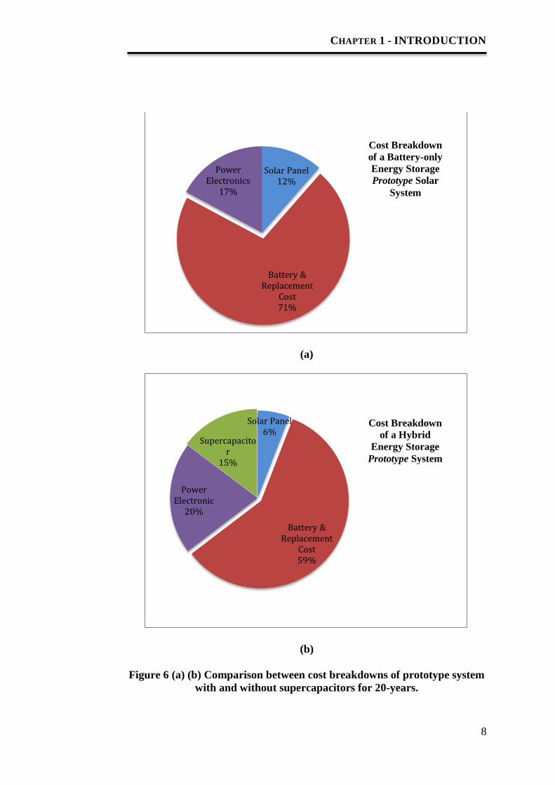
Figure 6 (a) (b) Comparison between cost breakdowns of prototype system
with and without supercapacitors for 20-years. ............................. 8
Figure 7 (a) (b) (c) Bi-directional dc-dc Converter from [17] ..................... 13
Figure 8 System Architecture for Prototype ................................................. 18
Figure 9 Battery Voltage Characteristics [25] .............................................. 24
Figure 10 Power Voltage Plot Comparison [25] ........................................... 24
Figure 11 Characteristics of the different charging algorithm ................... 26
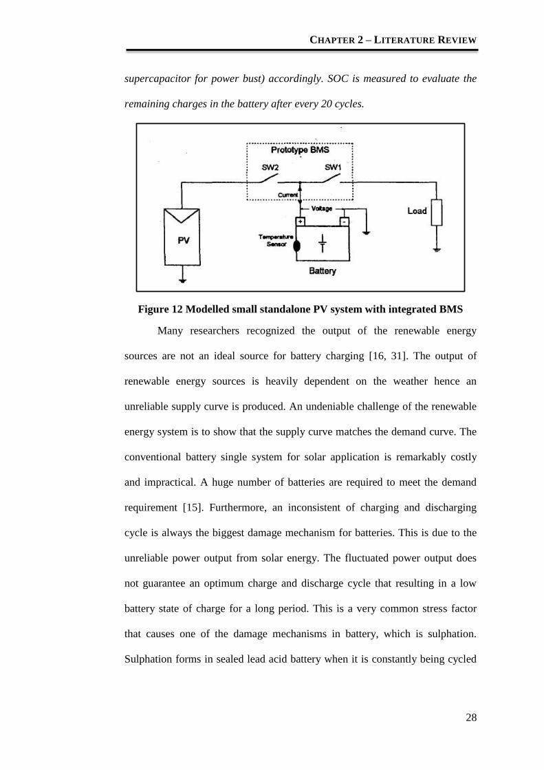
Figure 12 Modelled small standalone PV system with integrated BMS ..... 28
Figure 13 Battery discharge curves under different discharging rates ...... 32
Figure 14 Battery charging curves under different charging rates ............ 32
Figure 15 Chemical Reaction when a battery is being discharged ............. 35
Figure 16 Ragone plot ..................................................................................... 37
Figure 17 Electrochemical Double Layer Capacitor (EDLC) ..................... 39
Figure 18 Comparison of energy storage technology discharge / recharge
times ................................................................................................. 42
Figure 19 Charge – discharge profiles of a supercapacitor and a battery . 43
Figure 20 Topology of DC/DC converter ...................................................... 44
Figure 21 Current source of the photovoltaic system .................................. 46
Figure 22 Input and output voltage versus operating time of (a) buck
converters (b) boost converters (c) buck-boost converters with
supercapacitors ............................................................................... 47

LIST OF FIGURES
xi
Figure 23 Average output power versus the output voltage of (a) buck
converters (b) boost converters (c) buck-boost converters with
supercapacitors ............................................................................... 48
Figure 24 Normalised load current, battery current and supercapacitor
current .............................................................................................. 51
Figure 25 Block diagram of the power system suggested in [77] ................ 52
Figure 26 2D Hyperplane ................................................................................ 59
Figure 27 Mapping of data in Input Space to Feature Space ...................... 60
Figure 28 The Kernel Functions: (a) Polynnomial Function with p = 2 and
3; (b) RBF Function; and (c) Sigmoid Function. ......................... 61
Figure 29 Daily Electrical Load Profile ......................................................... 68
Figure 30 Capital cost vs. runtime for different energy storage devices .... 76
Figure 31 Architecture of HOMER software................................................ 81
Figure 32 GA Flow Chart ............................................................................... 94
Figure 33 Conventional Stand-alone renewable energy system with PV-
generator and diesel generator .................................................... 122
Figure 34 Supercapacitor-Battery Hybrid Energy Storage System (SB-
HESS) ............................................................................................. 124
Figure 35 Simulated Load Profile ................................................................ 129
Figure 36 Location for the hypothecial model ............................................ 134
Figure 37 Load Profile from HOMER ........................................................ 134
Figure 38 HOMER implementation of PV-Wind-Battery Energy System
......................................................................................................... 135
Figure 39 Average monthly solar radiation kWh/m2/day and clearness
index ............................................................................................... 137
Figure 40 Load profile ................................................................................... 155
Figure 41 Load profile for a prototype system ........................................... 168
Figure 42 (a) Supercapacitor Configuration, (b) Supercapacitor Bank on
prototype ........................................................................................ 175
Figure 43 (a) Battery Configuration, (b) SLA Battery Bank .................... 176
Figure 44 Schematic of control circuit prototype ....................................... 178
Figure 45 Control Circuit Prototype ........................................................... 179
Figure 46 Schematic of software control board .......................................... 180

LIST OF FIGURES
xii
Figure 47 Software Control Board............................................................... 181
Figure 48 (a) RC filter with 122 Hz cut off, (b) RC filter with 1.5Hz cut off
......................................................................................................... 182
Figure 49 RC filter performance comparisons ........................................... 182
Figure 50 Programmable load block diagram ............................................ 183
Figure 51 Programmable load ...................................................................... 184
Figure 52 Simulated load profiles ................................................................ 185
Figure 53 Time Response of Supercapacitor with Sequential Programming
......................................................................................................... 187
Figure 54 The 7-steps ahead load prediction .............................................. 189
Figure 55 Sparse Format in LIBSVM ......................................................... 191
Figure 56 Initial pattern 1 ............................................................................. 194
Figure 57 Initial Pattern 2 ............................................................................ 195
Figure 58 Algorithm of SVMR_EMS .......................................................... 198
Figure 59 British Standard IEC ................................................................... 202
Figure 60 Supercapacitor Electrode ............................................................ 205
Figure 61 Process of Lead Attachment using Ultrasonic Welder Machine
......................................................................................................... 206
Figure 62 Seperator ....................................................................................... 206
Figure 63 Cells and package ......................................................................... 206
Figure 64 Steps of supercapacitor Fabrication ........................................... 208
Figure 65 Autolab PGSTAT302N ................................................................ 212
Figure 66 Figure: Flow Chart of the Integrated Taguchi-GA method ..... 229
Figure 67 Integrated System on Trolley ...................................................... 231
Figure 68 Stress Test Load Profile ............................................................... 233
Figure 69 Circuit connection for MAXIM DS2438EVKIT+ ..................... 235
Figure 70 Meters screen of DS2438EVKIT+ .............................................. 235
Figure 71 Connections to simulate the charging and discharging phase of
the battery ...................................................................................... 236
Figure 72 Supercapacitor Respond Time .................................................... 237
Figure 73 Energy flow for battery-only and SB-HESS .............................. 245
Figure 74 Block diagram of PV-wind-battery energy system ................... 251

LIST OF FIGURES
xiii
Figure 75 Optimization result for PV-wind-battery system (0% of capacity
shortage) ......................................................................................... 251
Figure 76 Cash Flow Summary of PV-Wind-Battery System ................... 254
Figure 77 Electrical power for PV-wind-battery system (capacity shortage
0%) ................................................................................................. 255
Figure 78 Sensitivity results for PV-wind-battery system (capacity shortage
of 0%) ............................................................................................. 256
Figure 79 Electrical power for PV-battery system (capacity shortage of
0%) ................................................................................................. 257
Figure 80 Cash flow summary for PV-battery system (capacity shortage of
0%) ................................................................................................. 257
Figure 81 Optimization result for PV-wind-battery system (1% of capacity
shortage) ......................................................................................... 258
Figure 82 Electrical power for PV-wind-battery system (capacity shortage
of 1%) ............................................................................................. 260
Figure 83 Cash flow summary of PV-wind-battery system with capacity
shortage of 1% ............................................................................... 261
Figure 84 Sensitivity results for PV-wind-battery system (capacity shortage
of 1%) ............................................................................................. 262
Figure 85 Electrical power for PV-battery system (capacity shortage of
1%) ................................................................................................. 262
Figure 86 Cash flow summary for PV-battery system (capacity shortage of
1%) ................................................................................................. 263
Figure 87 Optimization result for PV-wind-battery system (2% of capacity
shortage) ......................................................................................... 264
Figure 88 Electrical power for PV-wind-battery system (capacity shortage
of 2%) ............................................................................................. 264
Figure 89 Cash flow summary for PV-wind-battery system (capacity
shortage of 2%) ............................................................................. 265
Figure 90 Sensitivity results for PV-battery system (capacity shortage of
2%) ................................................................................................. 266
Figure 91 Electrical power for PV-battery system (capacity shortage of
2%) ................................................................................................. 266

LIST OF FIGURES
xiv
Figure 92 Cash flow summary for PV-battery system (capacity shortage of
2%) ................................................................................................. 266
Figure 93 Cash Flow Summary for system with LPSP = 0 ........................ 278
Figure 94 Cost Summary for system LPSP = 0.1 and 0.2 .......................... 281
Figure 95 Cost Summary for PV-Battery system ....................................... 283
Figure 96 Cost Summary for PV-wind-supercapacitor-battery ............... 289
Figure 97 Cost Summary for PV-Supercapacitor-Battery System
(Prototype) ..................................................................................... 291
Figure 98 Comparison of number of batteries for Supercapacitor-battery
hybrid energy storage system and battery individual storage
energy storage system. .................................................................. 295
Figure 99 Predicted and Actual load for each load profiles ...................... 302
Figure 100 Graph of remaining battery capacity VS load cycle ............... 303
Figure 101 Graph of SOC in peak load VS load cycle ............................... 304
Figure 102 Graph of SOC in starting up load VS load cycle ..................... 304
Figure 103 Graph of SOC in steady state load VS load cycle ................... 305
Figure 104 Time Response of SVMR-EMS without load profile
identification .................................................................................. 306
Figure 105 Time Response of SVMR-EMS with load profile identification
......................................................................................................... 309
Figure 106 (a) Load prediction without load profile identification, (b) load
prediction with load profile identification .................................. 309
Figure 107 SVMR_EMS and Hardware approaches’ Supercapacitor
Response ......................................................................................... 310
Figure 108 Software approach’s power efficiency versus load ................. 311
Figure 109 (a) Original load profile, (b) Load profile affected by Battery
voltage level drop .......................................................................... 315
Figure 110 Voltage-Time plot from Galvanostatic charge-discharge test of
Sample CS16 at different currents (0.1, 0.2, 0.3 and 0.5 A) ...... 318
Figure 111 Capacitances of Sample CS16 at different currents (0.1, 0.2, 0.3
and 0.5 A) ....................................................................................... 318
Figure 112 Cyclic Voltammograms at various scan rates (2, 5, 10, 20mV/s)
......................................................................................................... 319

LIST OF FIGURES
xv
Figure 113 Capacitance plots of Sample CS16 at various scan rate (2, 5, 10,
20mV/s) .......................................................................................... 319
Figure 114 Overall capacitance of Sample CS16 at different scan rate (2, 5,
10, 20mV/s) .................................................................................... 320
Figure 115 Voltage-time plot from galvanostatic charge-discharge test of
Sample CS33 at different currents (0.1, 0.2, 0.3 and 0.5 A) ...... 320
Figure 116 Capacitances of Sample CS33 at different currents (0.1, 0.2, 0.3
and 0.5 A) ....................................................................................... 321
Figure 117 Cyclic Voltammograms at various scan rates (2, 5, 10, 20mV/s)
......................................................................................................... 321
Figure 118 Capacitance plots of Sample CS33 at various scan rates (2, 5,
10, 20mV/s) .................................................................................... 322
Figure 119 Overall capacitance of Sample CS33 at different scan rates (2,
5, 10, 20mV/s) ................................................................................ 322
Figure 120 Voltage-time plot from galvanostatic charge-discharge test of
Sample CS34 at different currents (0.1, 0.2, 0.3 and 0.5 A) ...... 323
Figure 121 Capacitances of Sample CS34 at different currents (0.1, 0.2, 0.3
and 0.5 A) ....................................................................................... 323
Figure 122 Cyclic Voltammograms at various scan rates (2, 5, 10, 20mV/s)
......................................................................................................... 324
Figure 123 Capacitance plots of Sample CS34 at various scan rate (2, 5, 10,
20mV/s) .......................................................................................... 324
Figure 124 Overall capacitance of Sample CS34 at different scan rates (2,
5, 10, 20mV/s) ................................................................................ 325
Figure 125 Capacitance for Supercapacitor Samples at different scan rates
......................................................................................................... 326
Figure 126 Charge and Discharge Curve .................................................... 329
Figure 127 Factor effects on WSNR ............................................................. 336
Figure 128 Percentage of SNR improvement after optimization as
compared to using OEC method.................................................. 344
Figure 129 Standard deviation comparison before & after optimisation
(Capacitance) ................................................................................. 345

LIST OF FIGURES
xvi
Figure 130 Standard deviation comparison before & after optimisation
(ESR) .............................................................................................. 345
Figure 131Schematic Solar Cabin ................................................................ 384
Figure 132 Power Electronics used in Solar Cabin .................................... 385
Figure 133 Batteries used in Solar Cabin .................................................... 385
Figure 134 Supercapacitor used in Solar Cabin ......................................... 385

LIST OF TABLES
xvii
LIST OF TABLES
Table 1 Comparison between Flooded Lead Acid Battery and SLA battery
................................................................................................................... 30
Table 2 Internal Resistance of Lead Acid Battery and Supercapacitor ..... 40
Table 3 Characteristics of Battery and Supercapacitor............................... 41
Table 4 Behaviour of ECU .............................................................................. 50
Table 5 Advantages and Disadvantages of SVM for Load Identification .. 62
Table 6 Kernels choices in LIBSVM .............................................................. 65
Table 7 Type of Load Forecasting ................................................................. 65
Table 8 Summary of Load forecasting techniques for STLF and VSTLF . 67
Table 9 Factors which affect the load demand ............................................. 67
Table 10 Drawbacks of various techniques in electricity load forecast ...... 73
Table 11 Publications on Optimization of PV and/or Diesel Hybrid Systems
with battery energy system. .................................................................... 89
Table 12 Comparison of natural evolution and genetic algorithm
terminology ............................................................................................ 102
Table 13 Performance of supercapacitor and lithium-ion battery ........... 110
Table 14 Methodology, justification and implementation steps ................ 115
Table 15 Methodology steps that contributes to Cost Reduction ............. 118
Table 16 Terms and Explanation for Equation 26 ..................................... 127
Table 17 Parameter data set for batteries ................................................... 128
Table 18 Theoretical Ucell (V) and Ubatt(V) Battery ................................... 129
Table 19 Energy demands of the electrical appliances .............................. 135
Table 20 Baseline Data for PV ..................................................................... 137
Table 21 Baseline Data for wind speed ........................................................ 139
Table 22 Advanced parameters for HOMER wind resource input .......... 141
Table 23 PV Panel Technical Parameters and Cost ................................... 143
Table 24 Wind Turbine-Technical Parameters and Cost .......................... 144
Table 25 Converter-Technical Parameters and Cost ................................. 144
Table 26 Specification of Hoppcake Battery ............................................... 145
27 Cost and Specification list of the components ........................................ 166
Table 28 Components and Data Specification for Prototype system ........ 171

LIST OF TABLES
xviii
Table 29 Roles of devices used in Prototype................................................ 177
Table 30 Data adjusted for 7 point ahead forecast ..................................... 190
Table 31 Data adjusted for Load Profile Classification ............................. 196
Table 32 Raw Material used in Supercapacitor Fabrication .................... 203
Table 33 Length and Width of the Electrode and Separator .................... 205
Table 34 Process factors and their levels for the supercapacitors fabricated
................................................................................................................. 219
Table 35 4 x L4 Orthogonal arrays for the process factors ........................ 220
Table 36 Data Specification of Battery ........................................................ 243
Table 37 Theoretical values for parameter Ibatt, Vcell, Vbat ........................... 244
Table 38 Indication for Optimization result in Figure 75 .......................... 251
Table 39 Net Present Cost of different RES (found by HOMER) ............ 268
Table 40 Fitness Function (Equation 27) ..................................................... 270
Table 41 Boundary of the Algorithm ........................................................... 271
Table 42 Six cases with different Battery DOD, capital and replacement
cost of the battery .................................................................................. 276
Table 43 Cash Flow Summary for the optimised system ........................... 277
Table 44 Comparisons between HOMER and GA ..................................... 278
Table 45 Optimization result for system with (LPSP = 0.1 and 0.2) ......... 279
Table 46 Cost Summary for the optimised LPSP = 1% and 2% system .. 280
Table 47 Optimization result for PV-Battery system with LPSP = 0 ....... 282
Table 48 Optimization result for PV-Battery system with LPSP = 0.1 and
0.2 ............................................................................................................ 282
Table 49 Cost Summary for PV-Battery system......................................... 283
Table 50 Fitness Function for RES with Supercapacitor and Battery ..... 284
Table 51 Fitness function for prototype with supercapacitor and battery
................................................................................................................. 285
Table 52 Boundary and Constraint for 2kW RES with SB-HESS ........... 286
Table 53 Optimization Result for RES with Supercapacitor and Battery287
Table 54 Cost Summary for RES with Supercapacitor and Battery ........ 288
Table 55 Boundary and Constraint for 72W prototype with SB-HESS ... 290
Table 56 Optimization Result for PV-Battery-Supercapacitor system .... 290

LIST OF TABLES
xix
Table 57 Cost Summary for PV-Battery-Supercapacitor system
(Prototype) .............................................................................................. 291
Table 58 Initial number of batteries and number of replacement battery
................................................................................................................. 295
Table 59 Optimised Net Present Cost (NPC) of RES found using the GA
................................................................................................................. 296
Table 60 Net present cost of RES using battery DOD 0.5 found using the
GA ........................................................................................................... 296
Table 61 Performance Definition of SVM ................................................... 299
Table 62 Performance Definition of SVR .................................................... 300
Table 63 Software approach power efficiency with various loads ............ 311
Table 64 Comparison of power efficiency with various loads ................... 312
Table 65 SVMR-EMS system cost ............................................................... 313
Table 66 Capacitance for Supercapacitors at different scan rate ............. 326
Table 67 Capacitance for Supercapacitors at different current ............... 326
Table 68 Experimental output data ............................................................. 329
Table 69 Weighted SNR (WSNR) Values .................................................... 331
Table 70 Optimal wc and wE ......................................................................... 333
Table 71 Main Effects on WSNR for every factor investigated of the
respective process .................................................................................. 335
Table 72 Experimental output data for confirmation experiments .......... 337
Table 73 SD for each experiment and under optimal conditions .............. 337
Table 74 OEC values to determine the optimal setting for the initial
condition ................................................................................................. 339
Table 75 Initial, predicted and actual improvement of SN ratio .............. 341
Table 76 Results of ANOVA analysis on WSNR ........................................ 343
Table 77 Project Objective and Achievements ........................................... 351
Table 78 Data obtained from Mixing Process. ............................................ 406
Table 79 Data obtained from Calendaring Process. ................................... 406
Table 80 Data obtained from Drying Process. ............................................ 406
Table 81 Data obtained from Electrolyte Treatment Process. .................. 406
Table 82 Data obtained from Assembling and Sealing Process. ............... 407

NOMENCLATURE
xx
NOMENCLATURE
GA Genetic Algorithm
SVM Support Vector Machine
RES Renewable Energy System
SOC State-of-Charge
DOD Depth of Discharge
O&M Operational and Maintenance
BMS Battery Management System
SLA Sealed-lead Acid Battery
SB-HESS Supercapacitor-battery hybrid energy storage system
SVMR_E
MS
Support Vector Machine/Regression Energy Management System
ESR equivalent series resistance
NPV Net Present Value
LCE Levelised Cost of Energy
NPC Net Present Cost
IC Intermittent Charging
TSC Three Stage Charging
ICC Interrupted Charge Control
EDLC Electric/Electrochemical Double Layer Capacitor
HESSS Hybrid Electrical Energy Storage Systems
ECU Electronic Control Unit
SRM Structural Risk Minimization
HYBRID2 The Hybrid Power System Simulation Model
GAMS The General Algebraic Modeling System
ORIENTE Optimization of Renewable Intermittent Energies with Hydrogen

NOMENCLATURE
xxi
for Autonomous Electrification
HOMER Micropower Optimization Model
PV Photovoltaic
LOLP Loss of Load Probability
LPSP Loss of Power Supply Probability
UL Unmet Load
ARES Advanced Reciprocating Engine Systems
WECS wind energy conversion system
HOGA Hybrid Optimization by Genetic Algorithm
ACS annualized cost of system
PSO Particle Swam Optimization
SOH State-of-Health
PbO2 lead dioxide
PbSO4 lead sulphate
Pb Lead
H2SO4 sulphuric acid
Ah battery capacity
UO Equilibrium voltage
g Electrolyte coefficient
ρ Internal resistance
M Transfer overvoltage coefficient
C Capacity coefficient
Voltage of the cell
Current of the battery
NREL National Renewable Energy Laboratory
Ucell
Ibatt

NOMENCLATURE
xxii
C.S.F capacity shortage fraction
STC standard test conditions
Ld Critical Discharge Power
CPV Capital cost of PV
CWG Capital cost of wind
CBAT Capital cost of battery
Ch Capital cost of wind generator per meter
CCH Capital cost of charge controller
yCH Estimated lifespan of charge controller
yINV Estimated lifespan of invertor
yp Lifespan of battery
CINV Capital cost of inverter
R Battery expected lifetime
NBAT number of batteries
the number of charge and discharge cycle
ECU electronic control unit
AR Autoregressive Technique
ARMA Autoregressive Moving Average
MAPE mean absolute percentage error
BPNN Back-propagation neural network
SRM Structural Risk Minimization
ACS annualized cost of system

CHAPTER 1 - INTRODUCTION
1
CHAPTER 1
INTRODUCTION
1.1 Overview
This thesis deals with using constraint optimization implemented using a
Genetic Algorithm (GA) for guaranteeing robustness in the manufacturing
process. A GA with a different objective function was also used to reduce the
implementation cost of supercapacitors in solar energy systems. This was done
by first fabricating supercapacitors of 22 Farad to be tested in a lab scale system
in order to establish the hypothesis that including supercapacitors in a Support
Vector Machine (SVM) hybrid battery energy management system increases
the operating lifespan of the battery in question.
These supercapacitors were fabricated in the Supercapacitor Pilot Plant
at the University of Nottingham Malaysia Campus using a Genetic Algorithm
to optimise Taguchi Signal-to-Noise ratios in order to obtain a more robust
supercapacitor better suited for solar application conforming to those standards
- IEC 62391 [1], IEC 62391-2-1 [2]. In actual fact, supercapacitors of 165F,
48V are used for 2kW solar applications, however in the supercapacitor pilot-
plant here, equipment to fabricate a supercapacitor of this size were not
available.

CHAPTER 1 - INTRODUCTION
2
(a)
(b)
Figure 1 (a) (b) Supercapacitor Pilot Plant
Developed by John Holland, Genetic Algorithms (GA) are general-
purpose global search and optimization methods applicable to a wide variety of
real life problems [3, 4]. GA are meta-heuristic search algorithms based on the
evolutionary ideas of natural selection and genetics [3, 4, 5, 6]. This means that
in meta-heuristic algorithms rules and randomness are combined to imitate

CHAPTER 1 - INTRODUCTION
3
natural phenomena. Furthermore, the GA is one of the most popular meta-
heuristic search algorithms that is used by many researchers to solve real-world
engineering optimization problems [3]. GA’s successfully overcome
deficiencies of conventional numerical methods [4] by intelligent exploitation
of the search landscape it passes thru [7]. It manipulates the population of
potential solutions through genetic operators that mimic the biological
evolution process, hence converging to an optimal solution [8, 9, 10]. Although
randomized during initialization, GA’s are by no means random; the algorithms
employ some form of selection to bias the search towards good solutions which
follows the principle of ‘survival of the fittest’ [11, 3]. It efficiently exploits
historical information gained from previous generations to directly search the
region where better (fitter) performing individuals lie within the search space
[9].
The Taguchi technique is used when a more robust product is needed
under volume manufacturing conditions [12, 13]. It is not used to obtain just
one ‘golden’ unit, but it is used to optimise the whole process for certain
parameters, which in our case is capacitance and equivalent series resistance
(ESR). Here robust and optimise means reproducible and consistent rather than
the biggest or smallest value.

CHAPTER 1 - INTRODUCTION
4
Figure 2 Fabricated Supercapacitor - Enerstora
Furthermore cells of 22 Farad, 2.3V were fabricated in a cylindrical
package in order to be used in the lab scale system for determining how much
battery life can be prolonged due to the presence of the supercapacitor.
(a)

CHAPTER 1 - INTRODUCTION
5
(b)
Figure 3 (a) (b) Lab Scale hybrid energy storage System
With this, it is hoped to prove that incorporating supercapacitors in an
energy management system, which contains a battery, will allow the battery to
have a longer lifespan due to it being able to stay at a higher state-of-charge
SOC) for a longer period of time. This result is reflective of the situation when
supercapacitors are included in energy management systems which operate at a
much higher voltage such as the one available at the University of Nottingham
Malaysia Campus (2kW solar cabin).
To further improve the performance of the implemented system on the
lab scale level while reducing its overall implementation cost due to power
electronics, the Support Vector Machine (SVM) was employed in the energy
control strategy. Basically, this enables a supercapacitor to be integrated into a
prototype hybrid energy storage system used for solar applications in an
economically feasible way. For large systems, such as the 2kW solar cabin,
based on the research carried out here, this saving is even greater. It is
approximately 36%.

CHAPTER 1 - INTRODUCTION
6
(a)
(b)
Figure 4 (a) (b) Comparison between cost breakdowns of A Hybrid Energy
Storage 2kW solar system with lab-scale prototype Hybrid Energy Storage
system
Solar Panel 11%
Supercapacitor
29%
Batteries 43%
Power Electronics
17% Cost Breakdown
of A Hybrid
Energy Storage
2kW Solar System
Solar Panel 19%
Supercapacitor
30%
Batteries 7%
Power Electronics
44%
Cost breakdown of
a prototype Hybrid
Energy Storage
System

CHAPTER 1 - INTRODUCTION
7
(a)
(b)
Figure 5 (a) (b) Comparison between cost breakdowns of 2kW system with
and without supercapacitors for 20-years.
Solar Panel 18%
Battery & Replacement
Cost 61%
Power Electronics
21%
Cost Distribution of
battery-only 2kW
Solar System for 20
years
Solar Panel 16%
Battery Replacement
Cost 24%
Supercapacitor
24%
Power Electronics
36%
Cost Distribution
of A Hybrid
Energy Storage
2kW Solar System
for 20 years
CHAPTER 1 - INTRODUCTION
8
(a)
(b)
Figure 6 (a) (b) Comparison between cost breakdowns of prototype system
with and without supercapacitors for 20-years.
Solar Panel 12%
Battery & Replacement
Cost 71%
Power Electronics
17%
Solar Panel 6%
Battery & Replacement
Cost 59%
Power Electronic
20%
Supercapacitor
15%
Cost Breakdown
of a Battery-only
Energy Storage
Prototype Solar
System
Cost Breakdown
of a Hybrid
Energy Storage
Prototype System

CHAPTER 1 - INTRODUCTION
9
The four previous pie charts in Figure 5 and 6 are the comparisons
between 2kW and the lab scale model for 20 years period. From the pie charts
shown above, conventional renewable energy system is not cost effective
mostly is due to the replacement cost of the batteries for long run. Replacement
cost of the battery often causes high impact on the total cost of the system. One
of focus in this project is to reduce the cost of replacement battery by
prolonging battery lifespan (about more than 5 years prolonged). Besides that,
the expensive power electronics to build the bi-directional converter in hybrid
energy storage system is eliminated by implementing an energy management
system which predicts load demand using SVM.
In relation to real life applications such as those that can be represented
by the 2kW solar cabin in this project, a GA with a new fitness function also
known as (objective function) was used to minimise the number of cost
components, which includes the initial cost of the components, operational and
maintenance cost in the proposed supercapacitor-battery hybrid energy storage
system. The proposed fitness function was proven to reduce the net present cost
of the system and improve the loss of power supply probability for a 20-year
round power system based on a comparison with a commercially available
software called Hybrid Optimization Model for Electric Renewable (HOMER)
[14].
In summary, the main motivation of this project is to incorporate a
supercapacitor within a solar energy system to minimise the cost in terms of the
number of batteries and the power electronics, subject to the constraint that the
load demand is completely covered, resulting in zero load rejection. One further
aim is to be able to propose a method of consistently manufacturing robust

CHAPTER 1 - INTRODUCTION
10
supercapacitor cells which are able to conform to the standards previously
mentioned. This aids in the cost reduction of the overall system by making the
supercapacitor cheaper to produce than the battery it replaces.
This research consists of three main components.
1. The first component in this project chiefly deals with a practical
methodology in tackling multiple-criterion optimization manufacturing
process by considering the advantages of both the Taguchi technique
and GA. The outcome of this part of the research is to achieve a robust
supercapacitor by searching the weighted signal-to-noise ratio as the
measure performance in relation to capacitance (C) and equivalent
series resistance (ESR) of a supercapacitor. It shows the robustness of
the fabricated supercapacitor is preferable than the commercial
supercapacitor according to the British Standard. The standard deviation
for the supercapacitor values (capacitance and ESR) is lower after the
process fabrication supercapacitor is optimised. – (this is presented in
Research Methodology Chapter 3, Section 3.3 and result shown in
Section 4.3.2 of this thesis).
2. The next component of the thesis focuses on the optimal sizing of the
proposed solar supercapacitor battery hybrid storage system using GA.
This proposed stand-alone solar system incorporates photovoltaic
panels, charge controller, a hybrid energy storage system and load. A
solar energy source is a clean and noise free source of electricity, even
so, a reliable energy storage system is required as an energy buffer to
bridge the mismatch between available and required energy. The
proposed energy storage technology employed in this project is the

CHAPTER 1 - INTRODUCTION
11
integration of lead-acid batteries (that acts as a main energy storage
device) and an auxiliary energy storage device which is the
supercapacitor. The proposed hybrid energy storage system leads to
system cost reduction. This is accomplished by reducing the number of
batteries and also the battery replacement costs by prolonging battery
lifespan. This is important, for example, in a common household load
profile, where there is certain intermittent demand for high current such
as when a motor starts up. This can be 6-10 times the normal operating
current of the motor and thus affects battery life [15, 16]. In a
conventional stand-alone solar system, lead-acid batteries are always
used to satisfy peak current burst. Other than reducing battery life, the
number of lead-acid batteries in this situation can be impracticable large
in order to match the peak current requirement. Non-optimal sizing of
the battery for this purpose is proven to be costly and not effective as
the peak current demand might only need to be met for a few seconds at
a particular time. Hence the need for an optimization strategy which
minimises the quantity of batteries while still satisfying the load
requirement. – (this is presented in Research Methodology Chapter 3,
Section 3.2.2 of this thesis).
3. The batteries in a conventional stand-alone solar system are replaced
typically every 3-5 years depending on the load demand curve [15, 16].
If not, an oversized battery system is suggested to cater for the peak
power and also to save the battery lifespan. Generally, this is due to
inconsistent battery charging by the solar energy source, as the output of
the source is heavily dependent on weather condition. The output of the

CHAPTER 1 - INTRODUCTION
12
solar energy source fluctuates according to the intensity of the light,
resulting an inconsistent battery charging and discharging cycle. Also,
heavy current discharging due to a heavy load requirement will equally
affect battery life.
The stress factor on the battery such as irregular discharging rate
and extensive time at the low state-of-charge (SOC) could increase the
rate of damage to the battery. The notable damage mechanisms are
related to battery electrolyte stratification and also irreversible
sulphation, which greatly shortens battery lifetime.
Ideas have been put forward to extend battery lifespan and
reduce battery quantity used in the system, where one solution is done
by pairing batteries with super capacitors as mentioned previous part.
When paired with supercapacitors, the former can act as a buffer,
relieving the battery of pulsed or high power drain, as well as reducing
the depth of charge discharge cycles by means of buffering. This idea
emerges because the supercapacitor has a greater power density than the
battery and this allows the supercapacitor to provide more energy over a
short period of time. Conversely, the battery has a much higher energy
density and this allows the battery to store more energy and supply to
the load over a longer period of time. Hence, the role of supercapacitors
is to supply sufficient energy for peak power requirements while the
role of battery is to supply continuous power at a nominal rate. – (this is
presented in Research Methodology Chapter 3, Section 3.2.3 and result
is shown in Section 4.2.3 of this thesis).

CHAPTER 1 - INTRODUCTION
13
Pairing supercapacitors and batteries however requires
expensive and extensive power electronics, elevating the already high
costs associated with these hybrid photovoltaic systems. Figure 7 [17]
shows the power electronics associated with conventional hybrid energy
system.
(a) Prototype bi-directional dc-
dc converter unit module
(b) The bi-directional DC/DC
converter(full-bridge type topology)
(c) Power stage design of converter unit module
Figure 7 (a) (b) (c) Bi-directional dc-dc Converter from [17]
There are however, other methods, which could be used in
developing these systems. For example, in this project the wide
availability and affordability of microcontrollers nowadays allows these
hybrid systems to be controlled using purely software methods such as
by employing the Support Vector Machine (SVM) pattern classifier to
decide when to switch energy sources depending on the load
requirement. The supervised learning system in SVM allows the

CHAPTER 1 - INTRODUCTION
14
prediction of load demand before it occurs. These aid in reducing the
delay in delivering power even when there are a few possible cases to be
considered in connecting or disconnecting battery and supercapacitor to
the load. This would not only lower the operational cost, but at the same
time, allows the hybrid photovoltaic system to be flexible, which comes
in handy in places with different seasons and unpredictable weather.
The implementation using a microcontroller also allows the monitoring
of multiple parameters, which may affect the efficiency of the hybrid
photovoltaic systems, optimising the operation of these systems by
taking appropriate actions when needed.
CHAPTER 1 - INTRODUCTION
15
1.2 Problem Statement
The main effort in this research is to solve the problem of combining
supercapacitors with batteries into a hybrid energy system which is made
economically feasible thru process and operational optimization using genetic
algorithms and the use of software in place of some of the power electronics.
Robustness of a product or process is important in increasing the yield
and the consistency of the product to make it economically feasible in the
application. The effort in robust design strategy for process fabrication of
supercapacitors is to make the supercapacitor insensitive to the probable causes
of performance variation. The goal of this component project is to determine
the optimal configuration of the supercapacitor process parameters that reduces
variation. In the proposed supercapacitor-battery hybrid energy storage system,
a robust process fabrication strategy eliminate those undesired spread in
capacitance values which can be attributed to several factors such as
manufacturing equipment tolerance, the temperature gradient in the system,
input material characteristics and cell aging. In most of power applications,
considerably high voltages are always required. However, the supercapacitor
has a low operational voltage, the maximum voltage that can be applied to a
supercapacitor is about 2.3V. To reach the required application voltage the
supercapacitors are connected in series or matrix to form a power system.
However, series connection leads to unequal voltage distributions because the
capacitance is not exactly the same for each device. In some cases this leads to
the use of balancing circuits which reduce the efficacy of the supercapacitor
bank. When balancing circuits are not used (sometimes to save operational
costs), the systems runs the risk of depleting the battery even more because the

CHAPTER 1 - INTRODUCTION
16
supercapacitor will act as an additional load when its voltage is lower than the
batteries nominal voltage.
Capacitance also varies with different DC bias voltages [18, 19, 20].
The change in capacitance with applied DC voltage (a phenomenon also known
as DC bias) further complicates the task of choosing the right capacitance.
Therefore, a manufactured supercapacitor, which has high reproducibility and
reliability, is crucial in maximizing the power reliability of the supercapacitor
after it is integrated in the power system to meet peak power demand.
Optimization the fabrication process of supercapacitors is a multi-
response problem, which involves optimising two output responses to improve
the product robustness. In optimising the fabrication process with the proposed
Taguchi-GA technique, inconsistent engineering judgment has been eliminated.
The limitation of the Taguchi Technique in performing well for multi-response
optimization problems has been overcome by formulating a way to include the
Genetic Algorithm within the Taguchi method. In previous research [21],
Vining and Myers presented a methodology within the framework of Taguchi’s
technique using Response Surface Method using a dual response approach. Del
Castillo and Montgomery [22] discussed that non-linear programming
solutions, i.e. Generalized Reduced Gradient algorithms can lead to better
solutions than those obtained with the dual response approach. Therefore, a
consistent optimization technique that eliminates engineering’s judgment is
important to obtain a set of optimised process parameters for fabrication
supercapacitor. This is to ensure small standard deviation of the supercapacitor
capacitance and voltage.

CHAPTER 1 - INTRODUCTION
17
Optimal sizing the supercapacitor-battery energy storage system for
solar application using GA is presented in Section 3.2.2. Again, consistent
values of capacitance and voltage are important for an optimised system
operation. This is because the optimal configuration of the system components
such as the number of solar panel, number of batteries, number of
supercapacitors and number of charge controller is determined based on the
specification of the components and the required design of the system.
Furthermore, the optimization algorithm is often constraint by the nominal
state-of-charge (SOC) batteries, power output of components and lifespan of
the components. A mismatch of the capacitance and voltage of supercapacitors
could activate and speed-up the damage mechanism of batteries. This is not
advantageous in the system as replacing batteries in the system is costly in the
long run. However, the optimization strategy proposed here also minimises the
number of batteries but it still able to bridge the mismatches between supply
and load demand when renewable energy sources are low. The system is also
able to deliver peak power without delay by coupling to an optimal number of
supercapacitors.
Another challenge in coupling supercapacitors and batteries is
implementing an energy management system to control the energy flow from
the hybrid energy storage system economically and accurately. A block
diagram depicts the system architecture for the implemented prototype is shown
in Figure 8.

CHAPTER 1 - INTRODUCTION
18
Figure 8 System Architecture for Prototype
To be able to compete with the efficiency and cost of other approaches
in balancing the voltage level of both battery and supercapacitor in the system
without delay, a load forecasting system using SVM and SVR is implemented
in the energy management system. The lead acid battery will be recharged
when its SOC reaches 80%. This is to improve the lifespan of the lead-acid
battery as its recommended Depth of Discharge (DOD) is 50%. Battery
supplies the continuous energy to meet the average load demand; while, the
supercapacitor provides instantaneous power to cater for the peak load demand.
The role of supercapacitor to meet peak load demand allows for the downsizing
of battery capacity, reducing the depth of discharge (DOD), reducing the
sulphation of battery, and most importantly, improving the battery’s lifespan
[23]. Hence, it’s crucial for the two storage banks to be switched ‘ON’ and
‘OFF’ at the right timing in accordance to the occurrence of peak load current
to achieve optimal performance. In this, the SVM-SVR will analyse the real

CHAPTER 1 - INTRODUCTION
19
time data of the system, perform classification, followed by regression to
predict the load currents, and perform the switching action efficiently.
1.3 Research Objectives
The main effort in this research is to solve the problem of combining
supercapacitors with batteries into a hybrid energy system which is made
economically feasible thru process and operational optimization using genetic
algorithms and the use of software in place of some of the power electronics. In
other words we aim to minimise operational cost of a solar system by
integrating supercapacitors into a hybrid lead acid battery energy management
system.
This can be accomplished by reducing the number of batteries used for
storage and extending battery life by allowing the supercapacitor to cater to
peak current demand. One further aim is to be able to propose a method of
consistently manufacturing robust supercapacitor cells which are able to
conform to the standards previously mentioned.
In supporting the main aims stated above, several research issues are to
be investigated and solved:
1. To identify and optimise the significant parameters of the fabrication
process simultaneously, by combining the Genetic Algorithm with
Taguchi DOE methodology and improving the Taguchi Signal-to-noise
Ratio which is a measure of product robustness.
2. To implement a fitness function which determines the optimal size (and
therefore reduce the cost) of a stand-alone hybrid supercapacitor-lead
acid battery solar energy system using a Genetic Algorithm.

CHAPTER 1 - INTRODUCTION
20
3. To design a supercapacitor-lead acid battery hybrid energy storage
system, which prolongs battery life and reduces the number of batteries
used.
4. To employ Support Vector Machine in the hybrid energy storage control
system in order to reduce the use expensive power electronic
components.
1.4 Scope of Research
This project covers and focuses on increasing product robustness and the
reduction of operational cost of a hybrid energy storage system consisting of a
supercapacitor and battery. It is not within the scope of this project to discuss
material improvements or the absolute improvement of capacitance and ESR
thru the materials or the process.
1.5 Thesis Structure
In Chapter 1, an overview, the objectives, and the scope of the project are
covered. The most important points are related to cost reduction issues for
hybrid solar energy systems. In chapter 2, the appropriate literature review is
presented. This chapter reviews the current state of the art for hybrid solar
energy storage systems in terms of the system configuration, the alternative
energy storage device, the optimization strategy, cost improvements and energy
management systems.
Chapter 3 covers the research methodology which was followed to fulfil
the objectives stated in this chapter which includes the improvements afforded
by the hybrid system as opposed to “battery only” energy storage strategies.

CHAPTER 1 - INTRODUCTION
21
Chapter 4 presents the result and discussion of the three main parts of
the project; the integrated Taguchi- GA method in process optimization; the
optimization of the system size for the complete hybrid renewable energy
storage strategy and the use of the SVM to predict load requirements based on a
certain LPSP (Loss of Power Supply Probability).
Finally Chapter 5, reviews the project objectives and discusses the
results obtained using the methodology prescribed in chapter 3. Potential future
work is also presented.

CHAPTER 2 – LITERATURE REVIEW
22
CHAPTER 2
LITERATURE REVIEW
This chapter reviews the current state of the art for hybrid solar energy storage
systems in terms of the system configuration, the alternative energy storage
device, the optimization strategy, cost improvements and energy management
systems.
2.1 System Configuration of Conventional Battery Single
Energy Storage System in Renewable Energy System (RES)
There have been a lot of researches being done to improve the practicability of
renewable energy generation systems. It appears to be common for renewable
energy generation systems to incorporate a storage element such as a battery to
complement the system. Several papers regarding the improvement on
renewable energy generation systems were reviewed and a brief description of
each paper are included below.
Ravinder Singh Batia, S. P. Jain, Dinesh Kumar Jain and Bhim Singh
conducted various simulations in their study titled “Battery Energy Storage
System for Power Conditioning of Renewable Energy Sources” to demonstrate
the role of an energy storage system. The aim of this study is to reduce the
transient voltage variations, load leveling, reactive power control and
harmonics elimination in renewable energy sources [24]. A controller has also
been included to manage the charging and discharging of the battery. The
modeled system however, does not include an element to buffer the rapid
charging and discharging of the battery as well as load buffering to protect the

CHAPTER 2 – LITERATURE REVIEW
23
battery, hence the battery is subjected to stresses which greatly reduce its
lifespan.
There are many types of battery technologies available. Niraj Garimella
and Nirmal- Kumar C. Nair examined the use of different types of batteries as
an energy storage system in small-scale renewable energy in the paper titled
‘Assessment of Battery Energy Storage Systems for Small Scale Renewable
Energy Integration’ [25]. A comparison of various characteristics has been
made between 4 types of batteries, which are lead acid, NiCd, NiMH and Li-
Ion batteries. It is found that NiMH and Li-Ion batteries have a faster rate of
increase in battery voltage and these batteries also reached their nominal
voltage in a faster time compared to lead acid and NiCd batteries. The power
output of the batteries were also compared and it is found that the NiMH
battery produces more power than the other batteries, while the lead acid and
NiCd type has similar power output whereas the Li-Ion have the lowest peak
compared to the other batteries, mainly because of its lower voltage value.

CHAPTER 2 – LITERATURE REVIEW
24
Figure 9 Battery Voltage Characteristics
[25]
Figure 10 Power Voltage Plot Comparison [25]
Figures 9 and 10 (Retrieved 28th
February 2011 [25]) show the
comparison of characteristics of different batteries. The study concluded that

CHAPTER 2 – LITERATURE REVIEW
25
Nickel-Metal Hydride batteries shows the best potential in terms of power
output, charge – discharge characteristics and voltage performance whereas
lead acid batteries are the most common and affordable for a small scale setup
among the other batteries [26, 25]. Hence, lead-acid batteries are chosen for
the primary energy storage devices in this project.
2.1.1 Conventional System configuration for Maximizing
Operating Lifespan of Batteries in Photovoltaic Systems
In the study titled ‘Recommendations for Maximizing Battery Life in
Photovoltaic Systems’, James P. Dunlop and Brian N. Farhi observed the use of
batteries in photovoltaic systems and made recommendations in issues related
to battery type and characteristics, system sizing, installation, operation and
maintenance as well as battery charge control in order to maximize the
operating lifespan of batteries used in photovoltaic systems [27].
Recommendations were made based on different battery types and trade-offs
between load availability and battery sizes as well as appropriate charge
controlling of different types of batteries, however, the study does not take into
account the use of buffering elements and the host of advantages it brings with
it. The use of buffering elements in these systems on top of the design tweaks
made based on the recommendations could further enhance the battery
operating lifespan in photovoltaic systems.
S. Armstrong, M.E. Glavin, W.G. Hurley in another study titled
‘Comparison of Battery Charging Algorithms for Stand-Alone Photovoltaic
Systems’ evaluates the effectiveness of different types of battery charging

CHAPTER 2 – LITERATURE REVIEW
26
algorithm namely, Intermittent Charging (IC), Three Stage Charging (TSC) and
Interrupted Charge Control (ICC) and their ability to maintain a high State-of-
Charge (SOC) [28]. The TSC was found to be the most suitable charging
algorithm for a regularly cycled battery in a photovoltaic system as the TSC
restored the battery’s SOC to 100% in the quickest time although there were
signs of overcharging. However, the TSC was found to cause the battery to
have a higher average temperature compared to IC and ICC, nonetheless, the IC
and ICC are only best utilized for standby applications [29].
SOC of the charging algorithms under the
absence of a load [28]
SOC of the charging algorithms under
varying load profiles [28]
Comparison of the charging efficiencies of
the charging algorithm [28]
Battery temperature during the
different charging algorithms [28]
Figure 11 Characteristics of the different charging algorithm
However, the charging algorithms do not take into account the use of
buffering elements during discharging phase, which further improves the

CHAPTER 2 – LITERATURE REVIEW
27
lifespan of batteries. In this project, only the discharging phase of the hybrid
energy storage devices (battery and supercapacitor) is considered. This was
done because the project addressed issues related to load rather than issues
related to device resistance or other factors that affected energy storage.
Battery individual energy storage system and Supercapacitor-Battery hybrid
energy storage system are compared in this research. It prolongs battery
lifespan and hence, improves system cost for the long run especially when the
replacement cost of batteries and operational/maintenance (O&M) cost are
taken into account.
In the paper titled ‘A Battery Management System for Standalone
Photovoltaic Systems’, Shane Duryea, Syed Islam and William Lawrance
outline the use of a Battery Management System (BMS), which consist of a
series solar regulator and a discharge protection to allow intelligent control of
charging and discharging of the battery in Photovoltaic Systems. The study also
analyses the various techniques in measuring the SOC of batteries, which
among others are methods based on Ampere-Hour Balancing with variable
losses and terminal voltage measurements. The BMS measures the SOC of the
battery to determine the available capacity, which enables intelligent control
schemes to be implemented to prolong battery lifespan [30]. The study however
does not take into account the use of buffering elements, which in turn limits
the prolonging of the battery operating lifespan in a PV system as well as the
host of advantages which comes with the use of a buffering element. Figure 12
[30] shows the model of the BMS integrated into a small standalone PV system.
In this project, the energy control management system monitors the voltage
drop of the batteries and microcontroller takes action switching on
CHAPTER 2 – LITERATURE REVIEW
28
supercapacitor for power bust) accordingly. SOC is measured to evaluate the
remaining charges in the battery after every 20 cycles.
Figure 12 Modelled small standalone PV system with integrated BMS
Many researchers recognized the output of the renewable energy
sources are not an ideal source for battery charging [16, 31]. The output of
renewable energy sources is heavily dependent on the weather hence an
unreliable supply curve is produced. An undeniable challenge of the renewable
energy system is to show that the supply curve matches the demand curve. The
conventional battery single system for solar application is remarkably costly
and impractical. A huge number of batteries are required to meet the demand
requirement [15]. Furthermore, an inconsistent of charging and discharging
cycle is always the biggest damage mechanism for batteries. This is due to the
unreliable power output from solar energy. The fluctuated power output does
not guarantee an optimum charge and discharge cycle that resulting in a low
battery state of charge for a long period. This is a very common stress factor
that causes one of the damage mechanisms in battery, which is sulphation.
Sulphation forms in sealed lead acid battery when it is constantly being cycled

CHAPTER 2 – LITERATURE REVIEW
29
at low state-of-charge (SOC). This is proven in [32, 33] that shorten the battery
lifespan.
This project shows that the supercapacitor-battery hybrid energy
storage system increases the practicability of the system which delivers power
without delay and reduces the initial number of batteries and number of
replacement batteries. It is also more environmental-friendly as most of the
composition in supercapacitor can be more biodegradable as compared to
battery.
2.1.2 System Configuration of Hybrid Energy Storage System
In this session, a buffer element is introduced – Supercapacitor (also known as
ultracapacitor) to pair with battery. Fuel cells with hydrogen tank is not
considered as an auxiliary energy storage device in this project as :
It is costly due to the electro-catalyst used at the anode faradic reaction
in fuel cells is expensive [34].
Furthermore, output voltage drops approximately 50% of its rated
voltage due to the second law of thermodynamics.
Production storage of hydrogen tank can be tedious and less mobility as
hydrogen has to be stored at pressure of 700atm in cylindrical-tanks. For
rural area, fuel cells is not a good option as travelling to replace
hydrogen tank in deep outskirt area is costly.
In the section below, some of the characteristics of the battery and
supercapacitor are presented to explain what motivates supercapacitor act as an
auxiliary energy storage device for our system. Furthermore, literature in this
section also focus on the topology of the converter and energy control system

CHAPTER 2 – LITERATURE REVIEW
30
that have been researched to control the energy flow between the two energy
storage devices. This section mainly covers the hardware approach and
software approach used to control the energy flow within hybrid energy storage
system which emerged repeatedly.
2.1.2.1 Battery
Based on the literature mentioned above, for solar charging application, the
energy storage choice favors batteries with deep cycle . Deep cycle batteries are
designed to have bigger plates and dissimilar chemistry to prevent the corrosive
effect when full capacity is frequently utilized [35].
Lead acid batteries, which offer deep cycles, large capacity and wide
availability is typically the choice for this application [15]. The comparison
between flooded lead acid battery which has higher heritage and the Sealed
Lead Acid (SLA) or VRLA battery are shown as below:
Table 1 Comparison between Flooded Lead Acid Battery and SLA battery
Flooded Lead Acid
battery
SLA battery
Cost Significantly less expensive Less expensive
Ventilation required YES NO
Maintenance YES NO
Potential liability Tipping or spilling NO
As shown in Table 1, the SLA battery is more costly as compared to
flooded lead acid battery. However, SLA battery is chosen as the energy storage
for its quality such as low capacity loss over time, maintenance-free, no
poisonous gas and acid fumes emission, and installation freedom [36, 37]. Since
SLA battery contains electrolyte that could last the life time of the battery, it

CHAPTER 2 – LITERATURE REVIEW
31
does not require watering as flooded lead acid battery do. The SLA also absorb
the hydrogen gas within itself, hence it could be recharge without much
ventilation. Lastly, SLA battery offers installation freedom as spilling will not
occur even if it’s overturned. On the other hand, SLA has shorter lifespan than
flooded lead acid battery and it can only be discharged to 50% SOC for
optimum performance unlike the flooded lead acid which could reach 80% [37].
Yet, the physical qualities has made SLA battery the better choice of energy
storage for solar application.
The lead acid batteries have relatively high energy density; however, it
does not have capability of instantaneous charging and discharging as those of a
supercapacitor [38, 39]. It could store much energy but it takes a longer time to
discharge and recharge. If it is driven at high C-rates especially in application
which requires a sudden load current burst, the lifespan of the battery will be
severely diminished. Besides that, high current drawing cause battery heat up
and possibly causing a fire hazard due to thermal runaway [40, 41]. The deep
discharge due to the large bust current drawn also cause the battery SOC to be
lowered. The low battery SOC causes to stratification and sulphation of the
battery, which reduces its lifespan [23, 27]. This is because the terminal voltage
decreases when the battery discharges to a load. A cut-off voltage or the
minimum allowable voltage is defined to designate the ‘empty’ state of the
battery. The cut-off voltage varies according to the type of battery and the
requirement of the application. In real life, a battery does not discharge in a
constant voltage due to the internal cell resistance, IR losses and polarization
effects of the electrodes [23, 42]

CHAPTER 2 – LITERATURE REVIEW
32
Figure 13 Battery discharge curves under different discharging rates
Figure 14 Battery charging curves under different charging rates

CHAPTER 2 – LITERATURE REVIEW
33
Figure 13 and Figure 14 (retrieved from [42] on December 2012) shows
the effect of different charging and discharging rate or current on the voltage
and the state-of-charge (SOC) of the battery. The C-rates shows the rate of
charging and discharging in Amperes in order to normalize against battery
capacity [42, 43]. For example, considering a battery of 100Ah, a C/5 rate
means that the battery will discharge at a discharging current of 20 in an hour.
As can be seen in Figure 14, ‘Rest’ means that where is no current flowing
through the cells which leads to no charging or discharging cycle occurring.
As the current moves through the battery cells, the battery voltage
reduces due to the internal cell resistance [42]. The cell’s voltage will increase
when there is current flow across the cell during the charging cycle. If the
charging rate or current is high, the voltage increases faster. For discharging
phase, the cell voltage drops due to the discharging current. As the discharging
rate or current increases, the battery’s voltage depression will be greater. This
theory is valid for all battery regardless of its type, size or environment [42].
These stress factors that happened on the battery have increased the rate of
damage mechanism of the battery. In the section below, damage mechanism
and stress factor of lead acid battery are explained.
Damage mechanism and stress factor of lead acid batteries
Battery lifespan is shorter in battery alone system due to the higher rate of the
damage mechanism within the battery [15, 32]. This is because the ageing
mechanism of the lead-acid battery results from various stress factors which
result from the performance characteristic of the energy storage systems. The
most crucial stress factors listed are [44, 23, 45]:
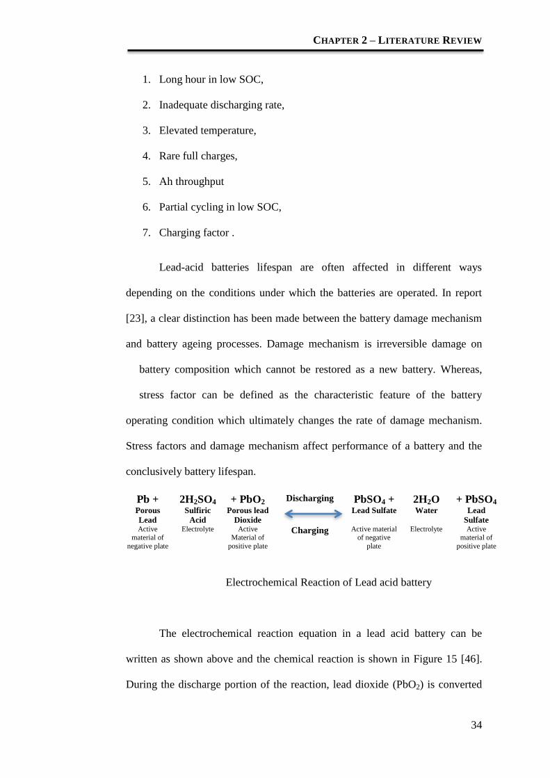
CHAPTER 2 – LITERATURE REVIEW
34
1. Long hour in low SOC,
2. Inadequate discharging rate,
3. Elevated temperature,
4. Rare full charges,
5. Ah throughput
6. Partial cycling in low SOC,
7. Charging factor .
Lead-acid batteries lifespan are often affected in different ways
depending on the conditions under which the batteries are operated. In report
[23], a clear distinction has been made between the battery damage mechanism
and battery ageing processes. Damage mechanism is irreversible damage on
battery composition which cannot be restored as a new battery. Whereas,
stress factor can be defined as the characteristic feature of the battery
operating condition which ultimately changes the rate of damage mechanism.
Stress factors and damage mechanism affect performance of a battery and the
conclusively battery lifespan.
Electrochemical Reaction of Lead acid battery
The electrochemical reaction equation in a lead acid battery can be
written as shown above and the chemical reaction is shown in Figure 15 [46].
During the discharge portion of the reaction, lead dioxide (PbO2) is converted
Pb + 2H2SO4 + PbO2 Discharging PbSO4 + 2H2O + PbSO4 Porous
Lead
Sulfiric
Acid
Porous lead
Dioxide Lead Sulfate Water Lead
Sulfate Active
material of
negative plate
Electrolyte Active Material of
positive plate
Charging Active material of negative
plate
Electrolyte Active material of
positive plate

CHAPTER 2 – LITERATURE REVIEW
35
into lead sulphate (PbSO4) at the positive plate. At the negative plate sponge
lead (Pb) is converted to lead sulphate (PbSO4). This causes the sulphuric acid
(2H2SO4) in the electrolyte to be consumed [45].
Figure 15 Chemical Reaction when a battery is being discharged
The idea of this supercapacitor-battery hybrid energy storage system
(SB-HESS) has put forward to
‘the less number of battery is discharged, the more frequently it is fully
charged; the more favourable is the effect on the lifetime of a lead acid
battery.’
Therefore, it is good to avoid deep discharge or over-discharge battery
[47]. This is done to reduce the impact of certain stress factors, such as the
forming of hard (or non-reversible) sulphation on the battery electrode [45],
shedding, active material degradation, electrolyte stratification and a small
impact on corrosion on the positive plate of the battery. In manufacturer
technical manual, it is often mention to avoid or disconnect the battery from the
load either electronically or manually when the end voltage (a function of the
discharge rate) is reached [47]. It is the voltage point at which 100% of the
usable capacity of the battery has been consumed or continuation of the
discharge is useless because of the voltage dropping below useful levels.

CHAPTER 2 – LITERATURE REVIEW
36
Generally, the final discharge voltage per cell depends on the battery discharge
rate and is given in battery data sheet. According to Power-Sonic [46], ‘deep
discharge’ is defined as one that allows the battery voltage under load to go
below the cut-off or (‘final’) voltage of a full discharge [46].
In most cases of typical RES, the batteries are stressed to supply power
peak at times resulting large current drawn from the battery in a short period.
However, in this approach, the battery discharge current is always fixed at a
nominal value based on the desired state-of-charge. State-of-charge (SOC) or
on the contrary depth of discharge (DOD) of battery indicates the remaining
amount of energy available expressed as the percentage of the rated energy
(SOC = 1 – DOD) [48]. In other words, SOC can also be defined as an
expression as the available present battery capacity (Ah) as a percentage of the
rated capacity (Ah) [49, 50], whereas, DOD can be explained as how deeply the
battery is discharged.
This idea is aided by coupling the supercapacitor. The power peak
deliveries are taken over mostly by supercapacitor and a small amount of
energy from battery. This brings benefits in delivering power peak on time
without delay and avoiding tremendous drain on the battery. With the
exception of temperature, a SVM (Support Vector Machine) energy control
system can favourably control all factors, so that the negative influence of
temperature can be reduced.
2.1.2.2 EDLC Supercapacitor
Many literature have been presented to explain what motivates coupling
supercapacitors with batteries to overcome the high depth of discharge of
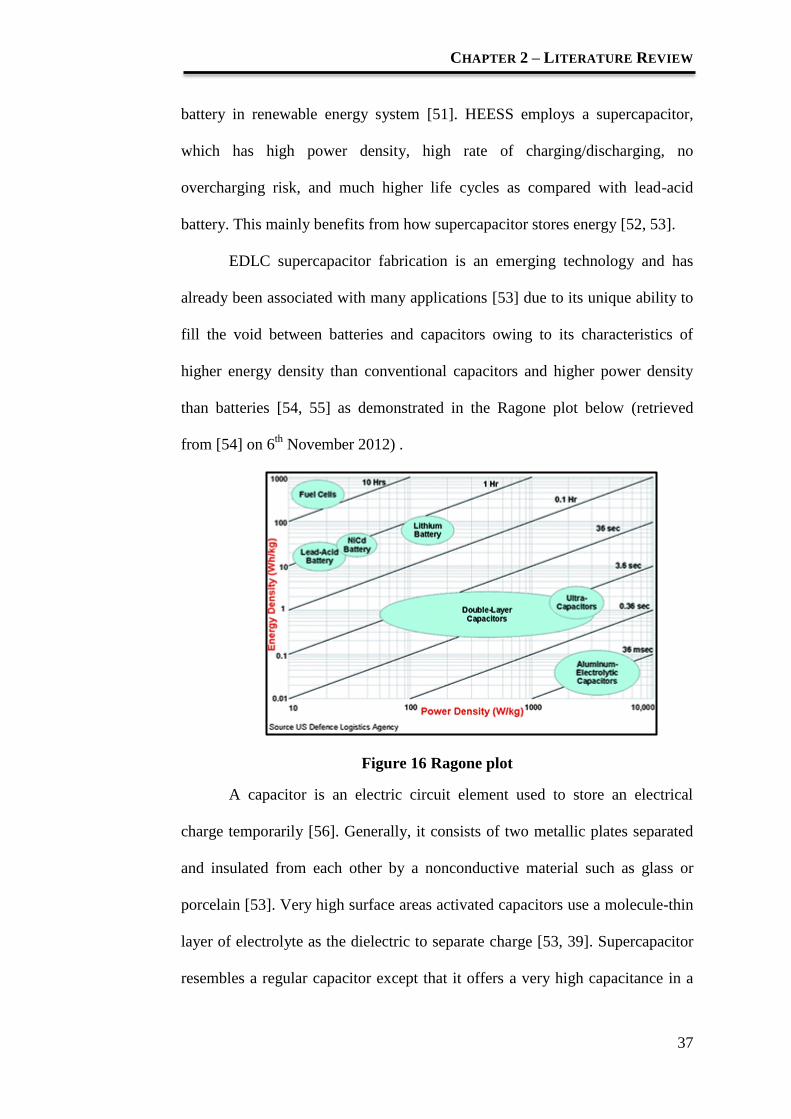
CHAPTER 2 – LITERATURE REVIEW
37
battery in renewable energy system [51]. HEESS employs a supercapacitor,
which has high power density, high rate of charging/discharging, no
overcharging risk, and much higher life cycles as compared with lead-acid
battery. This mainly benefits from how supercapacitor stores energy [52, 53].
EDLC supercapacitor fabrication is an emerging technology and has
already been associated with many applications [53] due to its unique ability to
fill the void between batteries and capacitors owing to its characteristics of
higher energy density than conventional capacitors and higher power density
than batteries [54, 55] as demonstrated in the Ragone plot below (retrieved
from [54] on 6th
November 2012) .
Figure 16 Ragone plot
A capacitor is an electric circuit element used to store an electrical
charge temporarily [56]. Generally, it consists of two metallic plates separated
and insulated from each other by a nonconductive material such as glass or
porcelain [53]. Very high surface areas activated capacitors use a molecule-thin
layer of electrolyte as the dielectric to separate charge [53, 39]. Supercapacitor
resembles a regular capacitor except that it offers a very high capacitance in a
CHAPTER 2 – LITERATURE REVIEW
38
small package. Energy storage is by means of static charge rather than of an
electro-chemical process inherent to the battery [34, 38, 39] The supercapacitor
is categorized into two groups: the electric double layer capacitor (EDLC), and
pseudo-capacitor, where both groups differs in the way they store the charges
[57]. The electrochemical supercapacitor stores the charges through the
reversible absorption of ions from an electrolyte on two porous electrodes [58]:
This creates an electric double layer at the electrode. EDLC is used in this
project due to its cycle life is higher than pseudocapacitor. It has about 5 times
more cycle life than pseudocapacitor [53, 59]. Additionally, the capacitance of
supercapacitor is dependent primarily on the characteristic (surface area and
pore size of the distribution) of the electrode material (such as carbon and
activated carbon) [53, 60]. These materials are cheap due to its wide
availability. This reduces the commercial price of supercapacitor in the market
as time goes [57]. However, the price of supercapacitor is still higher compare
to the price of battery. In this project, the idea of fabricating supercapacitors
with the desired capacitance and voltage is important to best-suits our
optimised system. This is a crucial step to further optimise the cost of the system
for a desired capacitance which might not be found in the commercial market.
EDLC does not involve chemical reaction, it merely absorb the ion in
physical means [41, 53]. Energy is stored in the double-layer capacitor as
charge separation in the double-layer formed at the interface between the solid
electrode material surface and the liquid electrolyte in the micropores of the
electrodes [53, 38, 39]. As shown in Figure 17 [55] , the EDLC can achieve up
to millions of life cycles as the charging and discharging process does not affect
the electrode physically [55] .

CHAPTER 2 – LITERATURE REVIEW
39
Figure 17 Electrochemical Double Layer Capacitor (EDLC)
The ions displaced in forming the double-layers in the pores are
transferred between the electrodes by diffusion through electrolyte. The
supercapacitor stores only a small amount of energy, yet it could deliver a rapid
power discharge which made it suitable for high rate of charging and
discharging operation.
where
εr is the electrolyte dielectric constant,
ε0 is the permittivity of a vacuum,
A is the specific surface area of the electrode accessible to the
electrolyte ions, and
d is the effective thickness of the EDL (the Debye length).
Equation 1
The energy stored can be calculated using the equation below:
Where
V is the cell voltage (in volts),
CT is the total capacitance of the cell (in farads)
Equation 2

CHAPTER 2 – LITERATURE REVIEW
40
The EDLC has high capacitance as shown in the Equations 1 [61, 38,
39] and 2 [61, 38, 39] above. The reason behind its high power delivery
capability lies in the fact that it has much lower internal resistance as compared
to the battery [38, 39]. The Table 2 shows the internal resistance of lead acid
battery and supercapacitor:
Table 2 Internal Resistance of Lead Acid Battery and Supercapacitor
Chemistry Internal Resistances
Lead Acid Battery 2-30mΩ
Supercapacitor 0.02-0.2mΩ
As shown in Table 2 [40], since the internal resistance of supercapacitor
is much lower than the battery the supercapacitor can supply a large burst of
current to the load while the battery will supply the lower continuous power for
a longer period of time. These properties complement the battery’s limitation
and allow the combination of SLA battery and supercapacitor in HEESS to
possess both high energy and power density [51].
As mentioned early, a supercapacitor (also known as a ultracapacitor) is
a double-layer electrochemical capacitor that can store thousands of times more
energy than a common capacitor [62]. It shares characteristics with both
batteries and conventional capacitors, and has an energy density [63] (the ratio
of energy output to its weight) approaching 20% of a battery [64, 65]. In other
words, a battery would have to be 80% heavier than the ultracapacitor in order
to produce the equivalent energy output.
Moreover, the supercapacitor is very rugged and has a life expectancy of
up to 50000 hours [15, 16]. This made it an ideal choice for remote solar
application where maintenance is difficult. Hence, HEESS extends battery

CHAPTER 2 – LITERATURE REVIEW
41
runtime, reduces the battery size, minimises space requirements, reduces the
pulse current noise and improve load balancing [56, 51]
In the HEESS formed by the supercapacitor and battery, their charging
time, self- discharging time, power and energy densities and efficiency is listed
in Table 3 [38, 15, 66]:
Table 3 Characteristics of Battery and Supercapacitor
Battery Supercapacitor
Charging Time Several Hours Fraction of seconds to
minutes
Self-Discharging Time Weeks to few
Months
Hours to Days
Energy Density 10-100Wh/kg <5 Wh/kg
Power Density <500W/kg >1000W/kg
Charging/Discharging
efficiency
70%-85% 85%-98%
This means that a supercapacitor is suitable to couple with battery in
situations where an instantaneous supply to power peak is required. It acts as a
buffer element to bridge the supply to load demand when the battery is
recharging [67, 16]. This hybrid system aims for zero load rejection. For
example, consider an application in an environment where frequent outages last
for less than two minutes. In such an environment, battery deterioration is
excessive due to the high frequency of the outages. Moreover, the battery tends
to require more time to recharge before it can supply to the next power peak.
This would result in a highly reliable energy storage system that would require
little or no maintenance. This is shown in Figure 18 [68].

CHAPTER 2 – LITERATURE REVIEW
42
Figure 18 Comparison of energy storage technology discharge / recharge
times
In short, supercapacitors are known as high power density storage
devices that allow instantaneous delivery of power peak. The ability of
supercapacitor to absorb and discharge large amount of energy in a short
period of time, supercapacitors make a great secondary energy storage device
especially in pulsed load applications, where a large amount of energy is
drawn in short periods of time. Hence, supercapacitors are the suitable device
to couple with battery in this project. Figure 19 [69] shows a comparison of the
galvanostatic charge – discharge profiles of a supercapacitor and a battery
under a similar duration where the supercapacitor discharges faster than battery
hence, allowing it to fulfill peak load demand.

CHAPTER 2 – LITERATURE REVIEW
43
Figure 19 Charge – discharge profiles of a supercapacitor and a battery

CHAPTER 2 – LITERATURE REVIEW
44
2.1.2.3 System configuration of Hybrid Electrical Energy
Storage Systems (HEESS)
In a HEESS, optimal design of the setup topologies between the supercapacitor
and battery has been the subject of many researches. Most conventional
approaches consider a direct parallel connection between the two storage banks
[70], a bidirectional DC/DC converter interfacing the two storage banks [15]
and dual input bidirectional DC/DC converter topology as shown in Figure 20
below [71, 72].
a) Topology of the passive parallel connection
b) Topology of the Bi-Directional DC-DC Converter
c) Topology of the Dual-input Bi-Directional DC-DC Converter
Figure 20 Topology of DC/DC converter

CHAPTER 2 – LITERATURE REVIEW
45
One of the challenge of coupling the supercapacitor and battery is the
different voltage level between the two different energy storage devices. A
conventional way of coupling supercapacitor and battery is connecting the two
devices in parallel. However, it reduces the capacity of the supercapacitor [51].
This direct approach maintains the same voltage over both sources but limits
the power delivered from the supercapacitor.
The single DC/DC converter controls the output current of the battery
and allows the supercapacitor to supply the extra power requirement to the load.
Lastly, the dual input bi-directional DC/DC converter give rise to highest
efficiency, reliability and flexibility [71]. However, it involves the use of more
costly DC/DC converters. Hence, the tradeoff between these topologies is the
cost of power electronics and efficiency of the HEESS.
Tatsuto Kinjo, Tomonobu Senjyu, Katsumi Uezato and Hideki Fujita
examined the use of Electrochemical Double Layer Capacitors (EDLCs) to
stabilize the output of a wind power generation system in the paper titled
“Output Leveling of Wind Power Generation System by EDLC Energy Storage
System”. The study uses an energy capacitor system which consists of an
EDLC and power electronic devices to compensate for the fluctuating power of
a photovoltaic system [73, 74]. The power electronic devices include a buck
boost DC – DC converter and a bi-directional inverter to complete the current
source of the photovoltaic system. Figure 21 [73] shows the current source of
the photovoltaic system:

CHAPTER 2 – LITERATURE REVIEW
46
Figure 21 Current source of the photovoltaic system
GD1 and D1 acts as a boost converter to charge the EDLC bank where
as GD2 and D2 acts as a buck converter to discharge the EDLC bank. The bi-
directional inverter in the other hand inverts the output from DC to AC. The
charging and discharging of the EDLC bank is controlled using a PI controller
[73, 74]. The system demonstrated above uses power electronics, which are
expensive electronic components especially in high-power applications.
In Harada, Sakau, Anan and Yamasaki’s research, an investigation of
the basic characteristic of the supercapacitors controlled by non-isolated DC-
DC converter has been done [75]. In the research, the operating time, energy
availability, input and output voltage and current were analysed.

CHAPTER 2 – LITERATURE REVIEW
47
Figure 22 Input and output voltage versus operating time of (a) buck
converters (b) boost converters (c) buck-boost converters with
supercapacitors
From the result obtained as shown in Figure 22 [75], it can be seen that
the maximum operating time of the buck-boost converter is the shortest
whereas the buck boost converter has the longest operating time under similar
conditions.

CHAPTER 2 – LITERATURE REVIEW
48
Figure 23 Average output power versus the output voltage of (a) buck
converters (b) boost converters (c) buck-boost converters with
supercapacitors
Figure 23 [75] shows the average output power versus the output
voltage of the non-isolated DC-DC converters with supercapacitors for different
energy availability. Energy availability is calculated from the output power
divided by the input power of the converter. The buck and buck boost
converter’s output power increases as the output voltage increases whereas for
boost converter, the output power is almost constant although the output
voltage increases .
From Harada, Sakau, Anan and Yamasaki’s research, it also can be seen
that the energy availability, η of the buck converter depends on the output

CHAPTER 2 – LITERATURE REVIEW
49
voltage and the number of supercapacitors connected [75]. However, for buck-
boost converter, the energy availability, η does not depend on the output
voltage and the number of supercapacitors [75]. To obtain high output power
from a buck converter, many units of supercapacitors are needed to be
connected in series in order to have higher voltage from the supercapacitor bank
compared to the output voltage of the DC-DC converter. This causes to a
problem of uneven charging due to the dispersion of capacitances of the
supercapacitors [75]. This causes to serious safety problem under British
Standard of IEC To overcome this problem, an additional voltage monitoring
and current bypass circuit is needed for each supercapacitor to keep the
balanced voltage [75].
M.E. Glavin, Paul K.W. Chan, S. Armstrong, and W.G Hurley, in the
study titled ‘A Stand-alone Photovoltaic Supercapacitor Battery Hybrid Energy
Storage System’, examined the role of an electronic control unit (ECU) in a
battery supercapacitor hybrid energy storage system under different load
conditions. The ECU is responsible in determining the State-of-Charge (SOC)
of the supercapacitor and battery and the supplying of energy to the load by
either the supercapacitor or battery with the aid of various sensors [16, 15] .
The proposed ECU had a behavior shown in Table 4 [15].

CHAPTER 2 – LITERATURE REVIEW
50
Table 4 Behaviour of ECU
The ECU mentioned was just a proposal and it was not stated that if the
ECU was software or hardware controlled. However, simulations showed that
the supercapacitor bank did increase the SOC of the battery under peak and
pulse current loads. This shows that the battery lifespan is not prolonged with
this strategy.
In the paper titled ‘Power and Life Extension of Battery – Ultracapacitor
Hybrids’, R. A. Dougal, Shengyi Liu and Ralph E. White investigated the peak
power enhancement and prolonged battery life of battery – ultracapacitor
hybrids over conventional systems. A simplified model was created to
analytically describe the performance of a battery – ultracapacitor hybrid power
source. Complementing a battery power source with ultracapacitor banks was
proven to greatly enhance peak power output, considerably reduces internal
losses and also prolongs the discharge life of the battery. Figure 24 [76] shows
No. Condition Action
1 PV Power = Load
(Battery SOC High) PV supplies load
No battery charging
2 PV Power = Load
(Battery SOC Low) PV supplies load
No battery charging
3 PV Power > Load
(Battery SOC High) PV supplies load
No battery charging
4 PV Power > Load
(Battery SOC Low) PV supplies load
PV charges battery
5 PV Power < Load
(Battery SOC High) PV supplies load
Battery supplies load
6 PV Power < Load
(Battery SOC Low) PV supplies load
Battery supplies load until
minimum SOC is reached then
shut down load
7 No PV Power
(Battery SOC High) Battery supplies load
8 No PV Power
(Battery SOC Low) Shut down load

CHAPTER 2 – LITERATURE REVIEW
51
the plot of the normalised load current, battery current and supercapacitor
current [76].
Figure 24 Normalised load current, battery current and supercapacitor
current
Observations from the plot shows that the during the load on-state, both
the battery and ultracapacitors (also known as supercapacitor) provides the
current consumed by the load while the during the load off-state, the battery
charges the ultracapacitor. The peak instantaneous current of the battery had
been greatly reduced with the assistance of the ultracapacitors, which would
otherwise have been the same as the output or load current. This greatly relieves
the battery off the peak stresses, reducing battery deterioration and positively
influencing the performance of the system [76].

CHAPTER 2 – LITERATURE REVIEW
52
2.1.3 Energy management of HEESS to Maximum Power
Transfer (load prediction)
J. C. Lima, A. Medeiros, V. M. Canalli, F. Antunes and F. S. Dos Reis
investigated the use of a neural network control system implemented on a PIC
microcontroller to track the maximum power point transfer between the load
and PV system in their study titled ‘A PIC Controller for Grid Connected PV
Systems using a FGPA based inverter’. A neural network is implemented on a
PIC to control the maximum output voltage in a DC-DC converter connected to
solar panels to obtain the maximum power transfer of the panels. The power
control is done to obtain the maximum power transfer which extracts the best
performance from the solar panel and is obtained through the control of the
duty cycle of the DC/DC boost converter, which supplies an adapted voltage to
a 3-phase inverter [77, 78].
Figure 25 Block diagram of the power system suggested in [77]
This implemented system shown in Figure 25 does not have an energy
storage system which can mitigate the problems associated with low-light
conditions.
Furthermore, high power rating electronic and complexity of designing
bi-directional converter cause impracticability of HEESS. In order to achieve
an efficient HEESS with lower cost, software based Energy Management

CHAPTER 2 – LITERATURE REVIEW
53
System (EMS) has been researched into. L. Gao, R. Dougal and S. Liu
presented the software approach which offers modularity, design simplicity and
reduces the reliance on power electronics [79]. Previous research in [80], had
shown a Sequential Programing based EMS which adopts the ‘Monitor and
Respond’ strategy but has shown unsatisfying results. This is due to the time
required in software approach to measure, process and respond accordingly. A
70ms delay was recorded in the respond of the supercapacitor after a peak load
current is monitored. This does not meet the performance requirement in small
DC machine, as the starting current is usually quite short in period. For
example, it’s measured that a 12 V, 1A DC motor load has a starting current of
only 5ms in duration [79]. Hence, the motor load will draw the large current
burst from the battery and causing the adverse effects on the battery as
mentioned earlier. In order to respond to this downfall of the software
approach, load prediction capability has to be integrated into the EMS in order
to match the respond of the supercapacitor with the performance required.
To implement the load prediction, the Support Vector Machine (SVM) is
researched into and it was applied in the prototype system. The SVM, a form of
supervised machine learning founded by V. Vapnik which is a non- parametric
statistical model based on Structural Risk Minimization (SRM) principle that
offers excellent generalization and predictive capability for limited sample size
[81]. Since the Load demand could be predicted by using recursive time series,
Support Vector Machine for Regression (SVR) was chosen to implement the
load prediction for its high generalization, single global minimum characteristic
and this will yield a good non-linear system model [82, 83].

CHAPTER 2 – LITERATURE REVIEW
54
In [84] Chang et al. proposed a SVR approach for the EUNITE Network
Competition which is the prediction of daily maximal electrical load of January
1999 based on temperature and electricity load demand (data used is from 1997
to 1998). It is interesting to mention that there is a periodic component within
the data set due to the seasonal variation of consumer electricity demand (such
as ‘holiday’ effects use of less electricity during major holidays) and the impact
of weather on electricity demand. Their inputs were several attributes, including
binary attributes for indicating which day of the week or holiday, etc. [85].
From these attributes, they formulated the predicted max load, which is a
numerical value. They concluded that the use of the temperature data did not
work as well because of the inherent difficulty in predicting temperature and
they also concluded that this SVR approach was feasible for determining an
accurate load prediction model. Chen et al. in [84] approach described in [85]
was the winning approach for the EUNITE Network Competition. These papers
[84] [85] described the SVM implementation. With respect to the design
details, it is interesting to note that the use of temperature in their model
actually decreases the accuracy of the predictions. This is due to the wide
variance of the output and resulting an improper temperature estimation [86].
Change et al. also experimented with data inputs excluding the previous (in
time series) load data. The result obtained shows unsatisfied performance. It is
worth to mention that the inputs to the SVR are not only time series load data
[86].
In [87], Zhang et al. discussed the use of SVM for short-term load
forecasting. The author stated that most linear models such as Kalman filtering,
AR (Autoregressive), and ARMA (Autoregressive Moving Average) models

CHAPTER 2 – LITERATURE REVIEW
55
are not typically sufficient to model the nonlinearities associated with short
term load forecasting processes. The use of SVR, with both electrical load data
and corresponding weather time series data, appears to outperform other neural
network (NN) based techniques including a back- propagation neural network
(BPNN). The authors also used cross validation to select the parameters for the
RBF kernel function as well as the regularization constant. The result obtained
shows that MAPE (mean absolute percentage error) of the SVM approach was
lower than that of the BPNN [87].
It appears that the reviews and studies conducted above show the
advantages of having an energy storage system in renewable energy systems.
The battery storage system could however be further enhanced using a
buffering element, in this research a supercapacitor, thus prolonging the
battery lifespan and reducing maintenance and operational costs at the same
time.
Moreover, a load forecasting-energy management system (using SVM)
aided with the use of sensors could be used in the supercapacitor-battery
hybrid energy storage system (SB-HESS) to achieve maximum optimization in
terms of system cost and power delivery. From the literature search mentioned
above, there is none of the energy management system that is implemented with
SVM load-predictive software to control the energy flow between the hybrid
energy storage devices and load.

CHAPTER 2 – LITERATURE REVIEW
56
2.1.4 Background theory of Support Vector Machine and
Support Vector Regression
2.1.4.1 Support Vector Machine for classification
The foundation of the Support Vector Machine (SVM) have been developed by
Vladmir Vapnik in year 1995. SVM has been gaining popularity over the 20
years due to many potential features and good empirical performance. The
Support Vector Machine is a form of supervised machine learning. SVM
formulation employs the Structural Risk Minimization (SRM) principle which
minimises an upper bound on the expected risk [88]; whereas the traditional
neural network or the ARIMA models which implement the Empirical Risk
Minimization (ERM) solely minimises the error on the training data [89]. SRM
principle that focuses on minimizing the upper bound of the generalization error
instead of minimizing the training error [90]. Implementing SVM classifier
with greater ability to generalize is often the ultimate foal in any classification
or pattern recognition task [91, 92]. The SVM optimises the network structure
through seeking the right balance between the Vapnik-Chervonenkis (VC)
confidence interval and the empirical error [89]. It is by bounding the
generalization error between the optimal balance of summation of training error
and the confidence interval term that a good generalization performance could
be achieved. Good generalization ability is an important characteristic of SVM
which is proven to perform better than neural networks under certain
circumstances [91]. The SVM also prevents overfitting as it perform well with
small training set. Besides that, SVM is equivalent to solving a linear
constrained quadratic programming problem which ensures a unique and global
optimal solution [93].
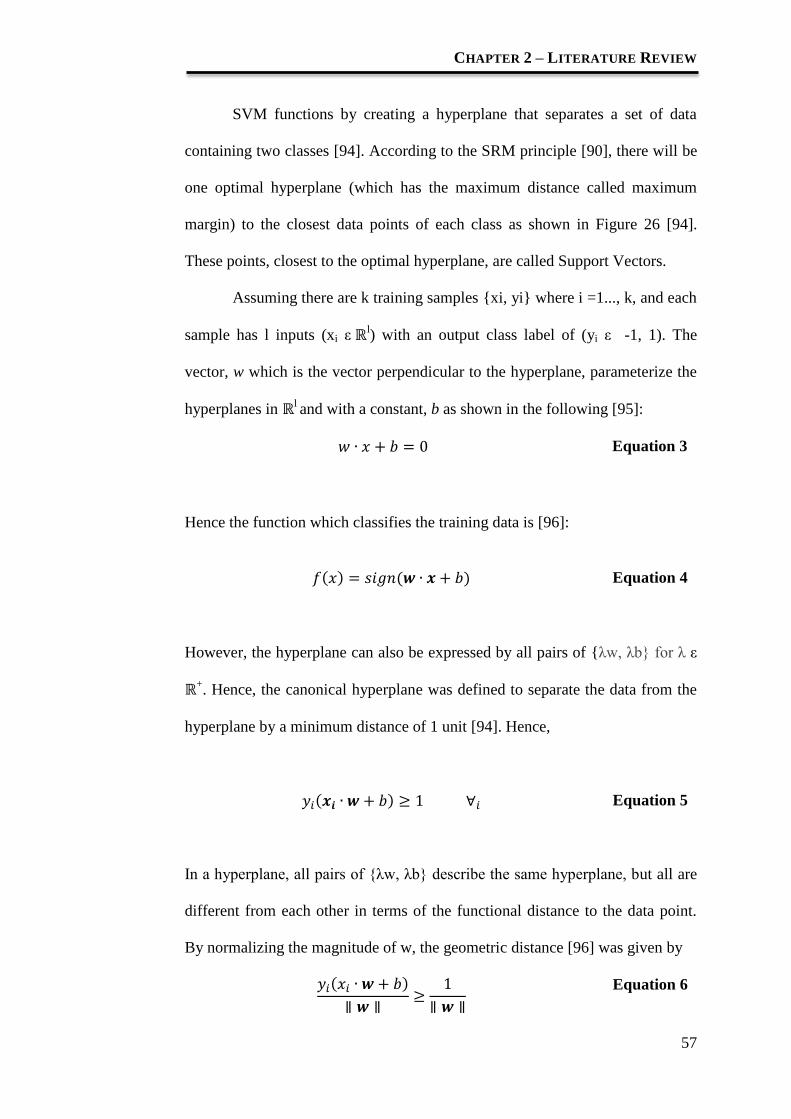
CHAPTER 2 – LITERATURE REVIEW
57
SVM functions by creating a hyperplane that separates a set of data
containing two classes [94]. According to the SRM principle [90], there will be
one optimal hyperplane (which has the maximum distance called maximum
margin) to the closest data points of each class as shown in Figure 26 [94].
These points, closest to the optimal hyperplane, are called Support Vectors.
Assuming there are k training samples xi, yi where i =1..., k, and each
sample has l inputs (xi ε l) with an output class label of (yi ε -1, 1). The
vector, w which is the vector perpendicular to the hyperplane, parameterize the
hyperplanes in l and with a constant, b as shown in the following [95]:
Equation 3
Hence the function which classifies the training data is [96]:
( ) ( ) Equation 4
However, the hyperplane can also be expressed by all pairs of λw, λb for λ ε
+. Hence, the canonical hyperplane was defined to separate the data from the
hyperplane by a minimum distance of 1 unit [94]. Hence,
( ) Equation 5
In a hyperplane, all pairs of λw, λb describe the same hyperplane, but all are
different from each other in terms of the functional distance to the data point.
By normalizing the magnitude of w, the geometric distance [96] was given by
( )
Equation 6
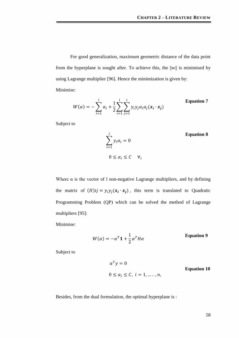
CHAPTER 2 – LITERATURE REVIEW
58
For good generalization, maximum geometric distance of the data point
from the hyperplane is sought after. To achieve this, the ||w|| is minimised by
using Lagrange multiplier [96]. Hence the minimization is given by:
Minimise:
( ) ∑
∑∑ ( )
Subject to
∑
Equation 7
Equation 8
Where α is the vector of l non-negative Lagrange multipliers, and by defining
the matrix of ( ) ( ) , this term is translated to Quadratic
Programming Problem (QP) which can be solved the method of Lagrange
multipliers [95]:
Minimise:
( )
Subject to
Equation 9
Equation 10
Besides, from the dual formulation, the optimal hyperplane is :

CHAPTER 2 – LITERATURE REVIEW
59
∑
Equation 11
when the functional distance of an data point is >1, then αi =0. Hence, only the
data point that lies on the margin has αi>0 which are required to define the
optimal hyperplane. These data points are called the support vectors. The αi is
also a measure of the data point weight in contribution to the hyperplane. To
find b, the positive and negative support vectors were used [90]:
Hence,
( )
Equation 12
Constructing a separating hyperplane in this feature space leads to a
non-linear decision boundary in the input space as shown in Figure 27 [94].
Expensive calculation of dot products in a high-dimensional space can be
avoided by introducing a kernel function, K below [92].
Figure 26 2D Hyperplane
When the soft margin constant, C= ∞ in Equation 10, the optimal
hyperplane will be able to separate all the data theoretically. Yet, with a finite C

CHAPTER 2 – LITERATURE REVIEW
60
the classifier is now a soft-margin which allows tradeoff between classifying all
data correctly with the complexity of the hyperplane model [96].
If the dataset is not linearly separable, it is like to be linearly separable
in the higher dimensional feature space [97]. This is done through the
introduction of kernel trick, where the input data was mapped into a higher
dimensional space. It is shown in Figure 27 below [98]:
Figure 27 Mapping of data in Input Space to Feature Space
The kernel which define the dot product in the higher dimensional
feature space as shown below [94, 96]:
Equation 13
Kernel function, K(xi, xj), plays an important role. In practice, various
kernel functions can be used [94] , such as
Linear:
Polynomial :
Radial Basis Function (RBF) :
Sigmoid:
K xi, x j( ) = F(xi ) ×F(x j )

CHAPTER 2 – LITERATURE REVIEW
61
The kernel function reflects the geometric relationship between the
input vector and the support vector, or the similarities of the features of the
faults.
For example [94], the polynomial kernel function in Figure 28 (a)
describes the similarity of the two vectors, since the dot product depicts the
canonical correlation. Choosing different order, p, would result in different
similarity measures and hence different results. The RBF kernel function, as
shown in Figure 28 (b), approximates the relationship between the two vectors
using a bell shape function. Tuning the parameter s would be similar to tuning
the covariance. The sigmoid kernel function in Figure 28 (c) is similar to the
polynomial kernel function. The parameters v and c can be used to adjust the
shape of the sigmoid function [99].
Figure 28 The Kernel Functions: (a) Polynnomial Function with p = 2 and
3; (b) RBF Function; and (c) Sigmoid Function.
Hence the classifying model is now
( ) (∑ ( ( )) )
Equation 14

CHAPTER 2 – LITERATURE REVIEW
62
As such, using the support vector machine (SVM) good generalization
is guaranteed and this will enable an efficient and accurate classification of the
sensor input data. This is appropriate to be used in this project to identify the
load pattern. Table 5 [100, 101, 102, 103] tabulates the advantages and
disadvantages of SVM for load identification.
Table 5 Advantages and Disadvantages of SVM for Load Identification
Advantages Disadvantage
It has high generalization and good
nonlinear modelling capability
which is suitable for time series
load prediction.
The adjustable penalty parameter
in SVM avoids the overfitting
problem. It also ensures a global
minimum output.
The use of soft margin classifier
gives better immunity to noise.
It has high efficiency in high
dimensional spaces; hence the
number of features of input vector
is not limited by the curse of
dimensionality.
It is effective in case when the
training samples size is smaller
than the number of
features/dimensions.
The computation requirement
depends on the support vectors
instead on the whole training data,
which yield a good processing and
memory efficiency.
The SVM decision function
depends on the kernel function,
which offers modularity. The
choice of kernel functions range
from the widely used common
kernel to specific custom made
kernel.
Poor performance is inevitable
when the number of sample is
very much smaller than the
number of features in the input
vector.
Cross-validation is used as
performance measure instead of
probability estimation, which
can hamper the performance.

CHAPTER 2 – LITERATURE REVIEW
63
2.1.5.2 Support Vector Regression (SVR)
The SVM was originally developed for pattern recognition task, however; with
the predictive capability of Vapnik’s ε-insensitive loss function it has been
extended into the nonlinear regression estimation domain [104, 105]. It has
been proven to exhibit excellent performance for time series forecasting [86].
The regression and classification task are similar.
For a training sample [106] :
( ) ( ) ( ) Equation 15
And the linear function f x):
( ) ( ) Equation 16
Hence, solve the optimization problem:
∑ (
)( )( ) ∑(
)
∑ (
)
Equation 17
Subject to
∑( )
Equation 18

CHAPTER 2 – LITERATURE REVIEW
64
By attaining the optimum value to get and the constant b
∑( )
Equation 19
∑( )
( )
Where
C is the regularization parameter, is the Gaussian kernal
function’s variance and ε is the insensitive loss function.
Equation 20
From this, the linear regression function can be constructed. To extend
this linear condition to non-linear domain, the use of kernel trick to transform
the input data into higher dimensional space, which solved the problem of curse
of dimensionality [106, 104].
LIBSVM
There are many tools available for implementation of the Support Vector
Machine. For example, Online SVR, Smooth Support Vector Regression
(SSVR), MATLAB in-built SVM toolbox, LIBSVM and such.
In this project, LIBSVM has been chosen for its well-established
library, update availability and its cross platform interfaces. It’s an integrated
program for SVM (C-SVC, nu-SVC), distribution estimation (one class SVM)
and regression (epsilon-SVR, nu-SVR) [102]. It also provides an efficient
multiclass SVM which is based on one-against-one approach which offer
shorter training time as compared with one-against-the-rest approach [103]. The
MATLAB extension of LIBSVM also allows the integration of the SVM, SVR,
Arduino Mega 2560, and MAXIM USB 6009 DAQ to run the SVMR-EMS, all

CHAPTER 2 – LITERATURE REVIEW
65
in one single MATLAB environment. The kernel choices offered in LIBSVM
[94]:
Table 6 Kernels choices in LIBSVM
Kernels name Kernels Equation
Linear
Polynomial
Radial Basis
Function RBF)
Sigmoid
Load prediction
Electricity Load forecasting plays a great role in modern energy management
system. An accurate load forecast helps eliminate the short transitional time
exists between the switching of power from the battery to the supercapacitor
bank. The predictive strategy in the energy management system predicts the
incoming load demand. This means the supercapacitor turns on before the real
power peak happens.
The Load Forecasting can be divided into four classes depending on the
utilized time frame and presented in Table 7 [107, 108]:
Table 7 Type of Load Forecasting
Forecasting Type [109]
1. Long Term Load Forecast (LTLF)
The time frame for this class used is typically 1 to 10 years; it focuses to
predict the load requirement for future power generation planning, line
building etc. Since the investment, designing and construction of power
plan takes up to decade long, this class of forecast is important for
meeting the demand in future.

CHAPTER 2 – LITERATURE REVIEW
66
2. Medium Term Load Forecast (MTLF)
The time frame for this class is typically within months to a year. The
load prediction focuses on meeting the medium term supply and capacity
constraint. Example, the load prediction is to match the supply with the
peak load demand in various seasons.
3. Short Term Load Forecast (STLF)
This class focuses on the load forecast of one day ahead. It is used to aid
the real time generation control and energy transaction planning.
4 Very Short Term Load Forecast (VSTLF)
This class focuses on the load forecast of hours and minutes ahead. It is
used to help the merchandizing and dispatch.
Most of the load forecast research paper focuses on the prediction of
maximum load demand. The research paper authored by Anthony Setiawan
[110] shows five minutes ahead VSTLF to set the production schedule of the
generators in Australia. The result for the prototype is shown in Section 4.2.2.3.
From the forecasted load, the generator and network operator will share their
maximum supply capacity with NEMMCO [111], and this enable the rest of
market player to react to meet the regional demand forecast. However,
maximum load demand prediction is not the main focus of this energy control
strategy. This energy control strategy success relies on its peak load prediction
capability within a short period of time in order for the supercapacitor to be
turned on before power peak. Hence, the load forecast for this project falls
under the VSTLF class with the objective for early detection of approaching
peak load to yield a good energy management response without any lag time.
Most research focuses on the STLF and a few of the research papers have
been focused on the VSTLF scope. Table 8 [110] below shows the summary of

CHAPTER 2 – LITERATURE REVIEW
67
load forecast techniques used for these two classes:
Table 8 Summary of Load forecasting techniques for STLF and VSTLF
Hence VSTLF is used in this load prediction system. To implement a
VSTLF, the factors that affect the electricity demand have to be understood.
They are listed as follows [112]:
Table 9 Factors which affect the load demand
Factors
1. Time
The time is an important factor that influences the load demand as it
relates to the routine and activities of a population. The electricity demand
differs from day to night, weekday, to weekends etc. However, a cyclic
nature is observable where the demand at different date but same time
and day is likely to be similar. This is important point as the previous
demand data could be used to predict the future demand.

CHAPTER 2 – LITERATURE REVIEW
68
A typical daily electrical load profile is shown in Figure 29. This figure
shows the peak in daily profile the opportunity for load prediction.
Figure 29 Daily Electrical Load Profile
As can be seen in Figure 29 [111], the load demand varies from time to
time within a day. Hence, it is greatly dependent upon the time variable as the
daily social and operating activities which consume electricity power are
mostly repetitive in nature. Others factor such as weather and random effect
will affect the load profile add more exogenous variable to the modeling
function. In this off grid PV system, the simulated load is used where it does
not have underlying factor such as random effect or weather effect. Hence, time
2. Random Effects:
In power system, the load demand is constantly subjected to random
disturbances of different scale. Sudden load variation could occur due to
operation of big motor machines, strike events and bad weather could lead
to oversupply as factories were shut down etc. All these add to the
difficulties of predicting the load demand.
3. Irregular Days:
In special day such as holiday or day with national event, the electricity
demand will see a fluctuation from the ordinary days.

CHAPTER 2 – LITERATURE REVIEW
69
and the previous load current values are the only variables that hold the relation
to the load demand output. It can also be observed that the relationship between
the time and the load demand is nonlinear in nature; hence the prediction
technique used will require good modeling of the nonlinear relationships.
In order to implement a VSLTF with good accuracy and speed, it is
crucial to select the suitable feature variables. The correlation factor between
the variable and the predicted output should be used as a measure of the
relevance of the variable. The conventional prediction technique using neural
networks has high number of parameters which require tuning and this causes
performance degradation. The load prediction using neural network is also
highly prone to overfitting problem. Overfitting describes the situation where
the training data yields good results but with fresh data the modal output is
erroneous. Hence, SVR which has only a few tuning parameters and does not
overfit can be used in place of neural network to achieve good result in load
prediction [109, 86].
Autoregressive modal of Time Series
The forecast technique consists of three main branches: The judgmental model,
Causal Method and Time Series Method. The first is a form of opinionated
prediction, which is not suitable for modeling the electricity demand. The
second is a prediction through constructing model which describes the
relationship between the dependent output variable to be forecasted and the
independent input variables. However, the implemented SVMR-EMS is an off
grid PV system, with the absence of any historical load data and the use of
programmable load to simulate the load, the variable that could relate to the

CHAPTER 2 – LITERATURE REVIEW
70
load current output are time and load current itself. Hence, the third
forecasting technique, the time series, specifically the autoregressive (AR)
modal is chosen for this task.
The autoregressive (AR) modal is a subset of the time series method
[86]. It’s a more specific type of the Autoregressive–moving average model
(ARMA) which represents a random process. However, the AR output
(dependent variable) is solely dependent linearly on its own previous values
only [113].
Hence, it is not capable of dealing with nonlinear model
representation in load forecast. Since SVR can perform well in the nonlinear
domain, the concept of AR was applied to SVR to approach the trend of load
demand.
Time series is a representation in time of a certain phenomenon. It is an
important physical phenomenon as most data holds time-dependent information
[86]. Time Series analysis is a problem of investigating the implicit system to
create a model for the time series data. On the other hand, Time Series
Prediction is the use of such model built with past historical data that could
forecast the future trend. It’s widely used for forecast in electricity load, stock
prices, weather etc. However, the main problems in modeling the time series
are non-stationary and noise. Noise Aspect refers the inadequacy of the past
data to reflect the dependency between the future and past in any time series.
The non-stationary refers to the relationship between input and output is
varying over time bit by bit [114]. Hence, the dynamics of recent data contains
more weight of information than the previous one [115].
The modeling of time series could be considered as regression problem
in a high dimensional input space more than one input feature (variable).

CHAPTER 2 – LITERATURE REVIEW
71
However, many time series problems regard the prediction of a sequence of
future data from the previous data only. This method is called multistep ahead
time series prediction. A single model is first constructed from past data of the
time series, and then it will be used stepwise for future values prediction. As the
predicted values will be used to predict the next value, this multi-stage
prediction/Recursive prediction is prone to error accumulation problem as has
been proven experimentally in the result section [116] . This prediction method
is normally used for long term load prediction and the model can be predicted
by iteratively using one-step-ahead prediction model [116]:
X( t +1) = F(X( t), X (t −1). . . X (t −m+1))
where F is the prediction model and m is the size of regressor.
Equation 21
By using the predicted value obtained in Equation 21, the next value can be
predicted using the same model [117],
X( t +2) = F(X (t), X( t −1). . . X( t −m+2)) Equation 22
For n iteration, the nth
prediction :
X (t +n) = F(X( t+n-1), X (t +n-2). . . X (t −m+n))
Equation 23
An alternative to the Multi-stage Prediction method for long term
prediction, called the independent value prediction which preserve the use
autoregressive modal, where previous variable value is used for predicting its
future value, yet it construct separate model for each prediction step. This

CHAPTER 2 – LITERATURE REVIEW
72
method is complicated in the sense that it requires many models to be
constructed to achieve the task [116].
Development of the K-step-ahead prediction:
For the SVMR-EMS, the load prediction is VSTLF; hence, being a short term
load forecast, it involves the use of one-step-ahead prediction as mentioned
earlier:
Y (t +1) = F(Y (t), Y (t −1). . . Y (t –m+1)) Equation 24
Yet, empirically, it was tested that SVMR-EMS failed to perform well
with just one step ahead prediction. The supercapacitor still turned ON after the
peak has passed, this implementation and experiment is proven in MEng
dissertation [118]. This is due to the processing time of SVMR-EMS for
classification and regression that require longer than the one-step-ahead buffer
time. Hence, to improve the load prediction capability of SVMR-EMS, K-step-
ahead autoregressive strategy, an improvised version of one-step-ahead
strategy was implemented.
Y (t +K) = F(Y (t), Y (t −1). . . Y (t −m+1)) Equation 25
This K-step-ahead autoregressive strategy will yield a predicted output
value which leads the actual load current (K* sampling time –processing time)
in advanced. This will ensure the SVMR-EMS to have good management
response. However, it creates certain shadow time in between the pattern
recognition to the output of the predicted value. During this short period of time
the SVMR-EMS will not be responsive to the load value. Hence, it is crucial for

CHAPTER 2 – LITERATURE REVIEW
73
suitable value of K to be chosen for the successful implementation of SVMR-
EMS.
Comparison of techniques for load prediction
The conventional techniques used for time series load prediction focuses on
statistical method and neural network. The former required the time series to be
steady, having normality and independence characteristic. Hence, it is not
suited for complex, nonlinear time series system [119]. The latter performs well
on nonlinearity, yet it suffers from overfitting, under fitting, and local minima
issues. In these, Autoregression and Moving Average (ARMA), Auto-
regressive Integrated Moving Average (ARIMA), Regression Models, Gaussian
Process (GP), Simplified Fuzzy Inference, Radial Basis Function Network
(RBFN), Multilayer Perceptron (MLP), Kalman filtering, Back Propagation
Neural Network (BPNN) was the techniques developed [120]. The ARIMA
model has been extensively implemented for seasonal time series predicting
models. Table 10 [86] below lists the models and their drawbacks in load
prediction:
Table 10 Drawbacks of various techniques in electricity load forecast
Forecasting
Techniques
Drawbacks in electricity load forecast
ARIMA
It lacks of flexibility for short term load forecasting as
the output state is dependent on the weighted sum of
previous states. Besides, the autoregressive model cannot
capture a nonlinear relationship in the output variable and
the previous values of the underlying variables whereas,
in load forecast, the time series are mostly nonlinear.

CHAPTER 2 – LITERATURE REVIEW
74
Regression Models Load forecasting is too complicated for Regression
Models which is widely used to predict the weather.
Gaussian Process
[121]
It is not sparse and required whole sample to perform
prediction. Besides, It has poor performance in high
dimensional space which limits the number of feature to
less than a dozen.
Artificial Neural
Network ANN)
such as MLP ,
BPPN and RBFN
It yields good nonlinear modeling for load forecasting
however, this techniques requires many parameters for
tuning, and need a large training sample and it will be
easily relapsed into local minima.
Kalman Filtering
[122]
Its error covariance matrix will not converge to adjacent
if the load demand sudden changes even though with
repetitive estimation.
The level of uncertainties in load forecasting has been upscale due to the
growth in intermittence generation such as Solar and Wind power generation in
smart grid system. This is due to the fact that intermittence generation suffers
from larger fluctuation of voltage magnitude and frequency as compare to the
traditional centralized electricity generation [119]. For this reason, more
sophisticated forecasting technique has to be used in place of the conventional
ones. Hence, the SVM which implements the structural Risk Minimization
Concept and has good generalization capability, good nonlinear modeling
feature of ANN and yields only a global minima output, has been selected for
performing the load forecasting task in this study [86].

CHAPTER 2 – LITERATURE REVIEW
75
2.2 Optimal Sizing of Renewable Energy System
The previous part of this chapter presents the system configuration for
conventional battery-individual system and system configuration of pairing
supercapacitor with battery in an energy storage system for solar application.
Various approaches to control energy flow in a hybrid electrical energy storage
system (HEESS) have been reviewed. In this section, review on different
optimization techniques and methodology optimal sizing for renewable energy
system are presented.
Conventionally speaking, lead-acid batteries are the main energy storage
device technology used in renewable energy systems (RESs) and autonomous
power-supply systems due to their maturity and low cost as mentioned in
Section 2.1, this factor will remain valid for the next few years. It is often
stated, however, that batteries in RES applications exhibit shorter lifetimes than
those expected by manufacturers’ data or those experienced in real applications.
Battery lifetime often alters with different load profile as this is closely related
to the ageing processes within a battery which lead to a loss of performance and
the stress factors which induce ageing and influence the rate of ageing [44].
Overall, in relation to all other components in RESs, the battery lifetime is
short. Adding the supercapacitor increases battery lifetime hence reduce costs.

CHAPTER 2 – LITERATURE REVIEW
76
Figure 30 Capital cost vs. runtime for different energy storage devices
The figure 30 [68] above shows the initial cost of the energy storage
devices. The capital cost is an important financial parameter, it should be
recognized that the total cost of ownership (which includes operational and
maintenance costs) is a much more meaningful index for analysis. For example,
the capital cost of lead-acid batteries is relatively low, however, they may not
necessarily be the least expensive option for environments experiencing
frequent outages of short duration. Under such circumstances, lead-acid
batteries will likely experience a shortened life span. Figure 31 is intended to
provide an overview cost comparison of different energy storage devices, it is
taken in [68].
On the other hand, lifespan for PV panels and wind generator are said to
be approximately 20 years however, lead acid battery has the shorter lifespan.
That being said, the efficiency of PV panel and wind generator degraded after
12 years, from 90% to 85% or 80% according to [123, 124, 125]. Furthermore,

CHAPTER 2 – LITERATURE REVIEW
77
battery lifespan has a distinct impact on the costs of the total system in the long
run. The cost of replacing batteries contributes a big portion in the overall cost
of the system for 20 years. In this project, supercapacitor-battery hybrid energy
storage system is implemented with the designed operation management system
(operation condition, set point SOC of battery) to prolong the battery lifespan.
Evidently, the cost for replacing the batteries is decreased throughout the 20
years.
In order to efficiently and economically utilize the renewable energy
resources and energy storage devices, an appropriate optimization technique is
required to accommodate all the number of parameters in this domain
(supercapacitor-battery hybrid energy storage system (SB-HESS) for solar
application). This area has been gaining interest from researchers and various
approaches were recommended by the researchers [48]. Generally, the aim of
this sizing is to determine the optimal configuration of the power system and
optimal location, type and sizing of generation units installed which subject to
constraint of the system meeting load requirements at minimum cost [126]. The
design of the hybrid renewable energy systems can be evaluated through its
lifetime cost and emission. The lifetime cost which subjects to the system
typically consists of two or more components. This means that the lifetime cost
of these components includes the capital, maintenance and operational cost.
Among all possible hybrid system configurations that are optimally dispatched,
the configuration with the lowest Net Present Value (NPV) is chosen as the
optimal configuration or it is called the optimal design [127, 128].
The common current optimal sizing tools are divided into two main
sessions. Firstly, software tools are commercially available that can be helpful

CHAPTER 2 – LITERATURE REVIEW
78
for real time system integration [129]. Secondly, there are number of
optimization techniques have also been applied by researchers for the sizing of
hybrid renewable energy systems [129] .
2.2.1 Commercially Available Software Tools
Commercial simulation programs are common tools to evaluate the
performance of the renewable energy systems. There are many energy tools that
can be downloaded from the websites of several research laboratories or
universities as mentioned in [129]. In [130], 68 energy tools and only 37 of the
energy tools were reviewed and used in energy analysis. These energy tools are
used for designing hybrid energy system such as the Hybrid Power System
Simulation Model (HYBRID2) [131] , the General Algebraic Modeling System
(GAMS) [132] , Optimization of Renewable Intermittent Energies with
Hydrogen for Autonomous Electrification (ORIENTE) [133], OptQuest [134,
135], LINDO [136] , WDILOG2 [137] , Dividing Rectangles (DIRECT) [138,
139], Determining Optimum Integration of RES (DOIRES) [140], Simulation
of Photovoltaic Energy Systems (SimPhoSys) [141], Geo-Spatial Planner for
Energy Investment Strategies (GSPEIS) [142, 143], Grid-connected Renewable
Hybrid Systems Optimization (GRHYSO) [144] and H2RES [145]. The authors
in [144] have developed the HOGA program (Hybrid Optimisation by Genetic
Algorithms), a program that uses a Genetic Algorithm (GA) to design a PV-
Diesel system (sizing and operation control of a PV-Diesel system). The
program has been developed in C++. A more detailed literature survey
specifically on commercially available software tools for the performance
evaluation of hybrid renewable energy systems in [130, 129].

CHAPTER 2 – LITERATURE REVIEW
79
By using the software program mentioned above, an optimum
configuration can be obtained by comparing the performance and energy
production cost of different system configurations. HYBRID2 simulates hybrid
systems with very high precision calculations, but it does not optimise the
system configuration [129]. TRNSYS (Transient Energy System Simulation
Program) was initially developed to simulate thermal systems. Besides that, PV
systems is also incorporated in this program to simulate hybrid systems,
however, this tool cannot be used to optimise the energy system configuration
[146]. Seeling-Hochmuth [144, 147] covers the optimization of PV-hybrid
energy systems. The hybrid control algorithm is simple, where the state-of-
charge (SOC) set point is the only parameter considered. Since there is no
detailed description of the GA, with the results being compared with those of a
simulation program (such as HYBRID2), this work can be considered to be in
the area of simulations and not in optimization of hybrid systems.
One of the most famous sizing simulation programs for renewable
energy system is HOMER, which developed by National Renewable Energy
Laboratory, United State [148, 129].
2.2.1.1 HOMER
HOMER is a user-friendly micro-power design tool developed in 1992 by the
National Renewable Energy Laboratory in the USA [14]. NREL released 42
versions of the program. It can be freely downloaded from [149]. According to
[130], there are more than 32,000 user have downloaded HOMER. HOMER is
a very user-friendly optimization program, a typical design and simulation can
be run after one day of training [130].

CHAPTER 2 – LITERATURE REVIEW
80
HOMER simulates and optimises stand-alone and grid-connected power
systems with any combination of wind turbines, PV arrays, hydro power,
biomass power, internal combustion engine generators, micro-turbines, fuel
cells, batteries, and hydrogen storage, serving both electric and thermal loads
(by individual or district-heating systems). All costs with any pollution
penalties (except fuel handling costs) and taxes are included in HOMER.
HOMER includes several energy component models, such as
photovoltaic, wind turbines, hydro, batteries, diesel and other fuel generators,
electrolysis units, and fuel cells, and evaluates suitable options considering cost
and availability of energy resources [150]. Grid connection is also considered in
HOMER design procedure. The software requires initial information before the
user run the simulation. Initial information such as energy resources,
economical and technical constraints, energy storage requirements and system
control strategies. Moreover, information on the components such as
component type, capital, replacement, operation and maintenance costs,
efficiency, operational life, etc. are also required [151]. The architecture of the
software is presented in Figure 24 [152, 153, 154, 130]. Sensitivity analysis in
HOMER could be done with variables having a range of values instead of a
specific number computed by the user [130].

CHAPTER 2 – LITERATURE REVIEW
81
Figure 31 Architecture of HOMER software
HOMER has widely been used in previous renewable energy system
case studies as presented for example in the literature [150, 155, 156, 157].
Both grid-parallel and stand-alone systems have been investigated using
HOMER. On the other hand, the parallel combination of renewable energy
sources and conventional systems such as diesel generators has also been
considered in many studies. These case studies are mentioned in papers [151,
128, 152, 153, 158]
In the literature mentioned above, researchers have shown optimum
sizing of hybrid systems using HOMER. A list of publications that involved
HOMER is available from its homepage [149]. HOMER has previously been
used to assess the wind energy potential at individual locations in Ethiopia
[158], to assess the feasibility of a stand-alone wind-diesel hybrid in Saudi
Arabia [151], to assess the feasibility of zero-energy homes [159] and simulate
a stand-alone system with hydrogen in Newfoundland, Canada [155]. Diaf et al.

CHAPTER 2 – LITERATURE REVIEW
82
[160] presented an application of hybrid PV–Wind– Battery systems (in
Corsica France) which minimises the Levelised Cost of Energy (LCE). Dalton
et al. [161] carried out the optimization minimization of NPC using HOMER
for a PV–Wind–Diesel–Battery system in Australia. In HOMER, total net
present cost (NPC) is used to represent the life-cycle cost of a system. The total
NPC condenses all the costs and revenues that occur within the project lifetime
into one lump sum in today’s dollars, with future cash flows discounted back to
the present using the discount rate. Himri et al. [162] optimised a wind–diesel
system using HOMER, with no batteries, to supply a remote village in Algeria.
In addition, simulations of the optimum system are carried out, using HOMER
and HYBRIDS for this purpose, comparing the simulations obtained with each
of the two programs [146].
HOMER considers 2 different types of control strategies .
1. Load-following Strategy [163, 150]: the diesel generator supplies power
to meet load demand at that moment only. Lower priority activities such
as, renewable sources are used to charge up the battery banks.
2. Charge-following Strategy [14]: The definition of the cycle charging
strategy is that whenever the generators run. The generators run at full
blast and charge the battery with any excess power. It works regardless
of the presence of, or value of, the set point SOC. But in the absence of
a SOC set point, HOMER will stop charging the battery. That might be
after only one time step. So without a set point SOC, the system
sometimes remains the battery at low SOC for a long time without
charging it up. That does not affect the simulation in HOMER at all, but

CHAPTER 2 – LITERATURE REVIEW
83
it could drain lead-acid batteries in real life. The battery set point state of
charge has no effect on whether HOMER charges the battery. The set
point SOC only affects how long HOMER continues to charge the
battery. The set point says that when the system starts charging the
battery, it will drain well continue doing so until the battery reaches the
set point SOC.
In HOMER simulation, control strategy on the system is also important.
It affectes the simulation result by changing the different type of control
strategy. The authors in [164], applied neural networks to the control strategies
of power PV–Diesel systems. Knowing the energy demand and the solar
irradiation, dynamic programming is used in order to optimise the operation of
the diesel generator and minimises the fuel costs. For this system, an adaptive
intelligence strategy is used. The authors also compared the results obtained by
applying two types of neural networks. In [165, 166] the authors proposed
various strategies for the operation of hybrid PV–Diesel–Battery systems. One
hour intervals are considered and the system parameters remain constant. They
also considered ideal batteries, without taking into account losses or the
influence of the cycles in the lifespan of the same. The three basic control
strategies proposed are the following [146]:
Zero-charge strategy (Load Following Diesel): the batteries are never
charged using the diesel generator. Therefore, the set point of the State of
Charge (SOC_Setpoint) is 0%.
Full cycle-charge strategy: the batteries are charged to 100% of their
capacity every time the diesel generator is on (SOC_Setpoint = 100%).

CHAPTER 2 – LITERATURE REVIEW
84
Predictive control strategy: the charging of the batteries depends on the
prediction of the demand and the energy expected to be generated by
means of renewable sources, so there will be a certain degree of
uncertainty. With this strategy, the energy loss from the renewable energies
tends to decrease.
The authors propose having an optimum point for the SOC_Setpoint
between 0% and 100% in such a way that the total operation cost of the system
is minimal. That is to say, the strategy will be between zero charge and full
cycle-charge.
In [165], the authors improved the control strategies model of [166] by
introducing new parameters that have become of great importance in the control
strategies of the software tools HYBRID2, HOMER, and HOGA [42]. The
Critical Discharge Power (Ld) is the value as from which the net energy (that
demanded by the charges minus that supplied by the renewable sources) is
more profitable when supplied by means of the diesel generator than when
supplied by means of the batteries (having previously been charged by the
diesel generator). The authors propose four control strategies frugal dispatch
strategy, load following strategy, SOC_Setpoint strategy and operation strategy
of diesel at maximum power (for a minimum time charging the batteries) [146].
In this research, HOMER is used to design and optimise battery-alone
system for solar and wind application. Result obtained from the established
Micropower Optimization Model (HOMER) is compared with the result
obtained from our implemented fitness function in the Genetic Algorithm (GA).
This is done to validate the implemented GA fitness function and the GA
program are working appropriate. Limitation in HOMER does not allow

CHAPTER 2 – LITERATURE REVIEW
85
optimal sizing of supercapacitor-battery hybrid energy storage system as the
software does not provide library for supercapacitor.
2.2.2 Other Optimisation Techniques
There are various optimization techniques such as the probabilistic approach,
graphical construction method and iterative technique have been proposed by
researchers [48]. Numerous papers have been written about the optimum
designs of PV and/or Wind and/or diesel systems with single energy storage in
batteries.
Generally, the optimum design in those papers reviewed were carried
out minimizing the Net Present Cost (NPC: investment costs plus the
discounted present values of all future costs during the lifetime of the system)
or by minimizing the Levelised Cost of Energy (LCE: total cost of the entire
hybrid system divided by the energy supplied by the hybrid system) [14].
Additionally, restrictions are usually included that are applied to reliability,
evaluating the same by means of one of the following parameters [146]:
Loss of Load Probability (LOLP): power failure time period divided by a
given period of time generally one (year).
Loss of Power Supply Probability (LPSP): probability that an insufficient
power supply will result when the hybrid system is unable to satisfy the
load demand.
Unmet Load (UL): non-served load divided by the total load of a period
of time normally one year).
Borowy and Salameh [167] presented a graphical construction method to

CHAPTER 2 – LITERATURE REVIEW
86
optimise the size of the PV generator and the capacity of the batteries in PV–
wind– battery systems. As initial data, the desired unmet load (UL) value is
considered. The required type of wind turbine, PV panel and battery are chosen
and fixed. By changing the number of photovoltaic panels and the number of
battery, systems that comply with the maximum UL value are achieved. In this
study [167], the systems are economically assessed, and the system with the
lowest cost is selected. This means that the system operation is simulated for
various combinations of PV array, battery sizes and based on the desired loss
of power supply probability (LPSP). For the desired LPSP, the PV array versus
battery size is plotted. The optimal solution with the minimal system cost is
chosen.
Another graphical technique has been given by [168] to optimise the
size of a hybrid solar–wind energy system by considering the monthly average
solar and wind energy values. However, in both graphical methods, only two
parameters for energy sources or energy storage device (either PV and battery,
or PV and wind turbine) were included in the optimization process [48].
Chedid and Saliba [169] proposed a method for the optimum design of
autonomous hybrid PV–Wind–Diesel–Battery systems by means of the
economic optimization of the system by applying lineal programming. Based
on literature review in [144, 146], Kaiser et al. presented a method to
simultaneously optimise the control strategies and the characteristics of the
elements of PV–Diesel–Battery systems, as well as online optimization of the
control strategy. Online optimization of the control strategy allows the
parameters to be redefined during the system operation based on decision-
taking theory.

CHAPTER 2 – LITERATURE REVIEW
87
Morgan et al. [170] described the Advanced Reciprocating Engine
Systems (ARES) program on simulation and optimization of hybrid PV–
Diesel–Battery systems, where the batteries are modeled with great precision.
Seeling-Hochmuth [147] carried out the optimization (minimization of the
NPC) of a hybrid PV–Wind–Diesel–Battery system by means of the Genetic
Algorithm technique. El-Hefnawi [171] presented an optimization method of
PV–Diesel–Battery systems. This method is based on the definition of a model
of a diesel generator, and from this, the optimum dimensioning of the PV
generator and of the batteries are obtained. On the other hand, Protogeropoulos
et al. [172] run the optimization of PV-Wind–Battery systems, modifying the
size of the batteries until a configuration that ensures sufficient autonomy is
achieved. Kellogg et al. [124] presented an iterative optimization method for
PV–Wind–Battery systems.
Elhadidy and Shaahid [173] have studied the effect of the size of the
batteries on the operation hours and on the energy provided by the diesel
generator in Wind–Diesel–Battery systems. The diesel back-up system is
operated at times when the power generated from wind energy conversion
system (WECS) fails to meet the load or when the battery storage is depleted .
The researchers in [173] showed that for economic considerations, for optimum
use of battery storage and for optimum operation of diesel system, storage
capacity equivalent to one to three days of maximum monthly average daily
demand needs to be used. It has been found that the diesel energy to be
generated without any storage is considerably high; however, the use of one day
of battery storage reduces diesel energy generation by about 35%; also the
number of hours of operation of the diesel system is reduced by about 52%.

CHAPTER 2 – LITERATURE REVIEW
88
Dufo-Lo pe and Bernal-Agust n [174] carried out the optimization of
hybrid PV–Diesel–Battery systems by using Genetic Algorithms (GA). In a
prior paper [175], they determined the correct performance of GA as a
technique for the design of hybrid systems. Thus, with the use of GA in , the
optimum or a very similar system to the optimum can be obtained with low
simulation and calculation time. The results obtained are compared in the
optimization of a hybrid system applying GA with the results obtained with an
enumerative method by assessing all the possible designs [175].
Koutroulis et al. [176] presented a paper for economic optimization by
means of Genetic Algorithms on PV–Wind–Battery systems. Shaahid and
Elhadidy [177] used the HOMER software for the economic optimization. The
authors in [177] minimised the NPC of a PV–Diesel–Battery system to supply a
shopping center located in Dhahran Saudi Arabia. Ashok [178] presented an
optimization method for PV–Wind–Diesel–Battery systems that includes
microhydro. The LCE of all of the possible component combinations is
assessed in [178]. It is applied to an example located in India. Diaf et al. [160]
presented an application of hybrid PV–Wind– Battery systems in Corsica
France), which minimises the LCE. Table 11 [146] shows a summary on the
optimization of renewable energy system

CHAPTER 2 – LITERATURE REVIEW
89
Table 11 Publications on Optimization of PV and/or Diesel Hybrid Systems
with battery energy system.
2.2.2.1 Optimal sizing RES using GA
GA has been widely used in renewable energy system sizing studies due to
certain advantages. As mentioned earlier, Koutroulis et al. [174, 156, 176],
Yang et al. [48, 179] and Bilal et al. [180] utilized GA for sizing of a stand-
alone hybrid PV-Wind system. Lagorse et al. [181] applied a hybrid GA and
simplex-based methodology to economically design a multi-source hybrid unit
composed of PV, wind generator, fuel cell. In [129], a more comprehensive
system consisting of PV, wind, fuel cell, microturbine, and battery was
optimally sized using a GA. Lopez et al. developed a simulation program
named HOGA (Hybrid Optimization by Genetic Algorithm) based on
utilization of a GA in order to design different optimal combinations of
autonomous hybrid energy systems including a diesel generator as backup in
[174, 182]. GA was also utilized in other different cases of energy system
sizing studies based on [183, 184, 185, 186, 187, 188, 189, 190].

CHAPTER 2 – LITERATURE REVIEW
90
Tina et al. [191] presented a probabilistic approach based on the
convolution technique to incorporate the fluctuating nature of the resources and
the load, thus eliminating the need for time-series data, to assess the long-term
performance of a hybrid solar–wind system for both stand-alone and grid-
connected applications.
A graphical construction technique for determining the optimum
combination of battery and PV array in a hybrid solar–wind system has been
presented by Borowy and Salameh in [167]. The system operation is simulated
for various combinations of PV array and battery sizes and the loss of power
supply probability (LPSP). Then, for the desired LPSP, the PV array versus
battery size is plotted and the optimal solution, which minimises the total
system cost, can be chosen. Another graphical technique has been given by
Markvart [168] to optimise the size of a hybrid solar–wind energy system by
considering the monthly average solar and wind energy values (input and
output). However, in both graphical methods, only two parameters (either PV
and battery, or PV and wind turbine) were included in the optimization process.
Yang et al. in [192] have proposed an iterative optimization technique
following the loss of power supply probability (LPSP) model for a hybrid
solar–wind system. The number selection of the PV module, wind turbine and
battery ensures the load demand based on the power reliability requirement
(desired LPSP) and the system cost is minimised. Similarly, in [124] an
iterative optimization method was presented by Kellogg et al. to select the wind
turbine size and PV module number needed to make the difference of generated
and demanded power as close to zero as possible over a period of time. From
this iterative procedure, several possible combinations of solar–wind generation

CHAPTER 2 – LITERATURE REVIEW
91
capacities were obtained. The total annual cost for each configuration is then
calculated and the combination with the lowest cost is selected. This represents
the optimal configuration for the system.
Eftichios Koutroulis et al. [176] proposed a methodology for optimal
sizing of stand-alone PV/WG systems. This proposed methodology suggests
(among a list of commercially available system devices) the optimal number
and type of units ensuring that the 20-year round total system cost is minimised
subject to the constraint that the load energy requirements are completely
covered, resulting in zero load rejection. It means the authors finds the global
optimum system configuration with relative computational simplicity.
However, the configurations are not always cost effective. This is due to the
small amount of load rejections are actually tolerable in order to gain an
acceptable system cost. Since this is a zero load rejection system, this
optimization algorithm has the potential of searching the oversized system.
A common disadvantage of the optimization methods described above is
that the proposed methodology do not mention the best compromise point
between system power reliability and system cost. The minimization of system
cost function is normally implemented by employing probability programming
techniques or by linearly changing the values of corresponding decision
variables, resulting in suboptimal solutions and increased computational effort
requirements [48]. Also, these sizing methodologies normally do not take into
account some system design characteristics, such as PV modules slope angle
and wind turbine installation height, which also affect the resulting energy
production and system installation costs.

CHAPTER 2 – LITERATURE REVIEW
92
In this paper [48], one optimal sizing model for a stand-alone hybrid
solar–wind system employing battery banks is developed based on the loss of
power supply probability (LPSP) and the annualized cost of system (ACS)
concepts. The optimisation procedure aims to find the configuration that yields
the best compromise between the two considered objectives: LPSP and ACS.
The decision variables included in the optimisation process are the PV module
number, wind turbine number, battery number, and also the PV module slope
angle as well as the wind turbine installation height. The configurations of a
hybrid system that meets the system power reliability requirements with
minimum cost can be obtained by applying an optimization technique such as
the genetic algorithm (GA). It is said to be an advanced search and optimization
technique in [179]; it is robust in finding global optimal solutions, particularly
in multi-modal and multi-objective optimisation problems, where the location
of the global optimum is a difficult task [129].
2.2.3 GA acts as an Optimal Sizing Algorithm
This part of review focuses on benefits of using the Genetic Algorithm (GA) in
sizing renewable energy system instead of the theory of GA.
GA is an optimisation method based on the genetic process of biological
organisms [193, 194].By mimicking this process, GA provides solutions to
complex real world problems. The concept of GA was firstly proposed by
Holland [5] and then widely utilized in many types of applications.
In the review paper [129], the input data of GA-based methodology is
listed as follows:

CHAPTER 2 – LITERATURE REVIEW
93
1. The meteorological conditions.
2. The unit prices of the projected hybrid system components including
installation and maintenance costs.
3. Some constraints can also be added to the algorithm. Example constraints
can be given as limiting the maximum number of PV panels on a building
roof that is constrained by roof area, limiting the number wind turbines
installed on specific land constrained by land area, or limiting the power
change slope of a fuel cell, etc. Many different constraints can be defined
due to the type and preferences of application.
4. A fitness function must be defined as an input to the GA approach. This is
the crucial highlight for this method.
5. The parameters for GA operators such as the percentage of selection and
rate of mutation should be provided before the GA-based sizing process
starts.

CHAPTER 2 – LITERATURE REVIEW
94
Figure 32 GA Flow Chart

CHAPTER 2 – LITERATURE REVIEW
95
With the given input data, GA sizing methodology provides an iterative
procedure utilizing the GA operators until a predefined termination criteria or
maximum iteration number are reached.
Briefly, a basic GA consists of five components. These components
represents a random initial population generator, a ‘fitness’ evaluation unit and
genetic operators for ‘selection’, ‘crossover’ and ‘mutation’ operations [193,
194, 195]. With the random population generation at the beginning, GA hence
initiates random population for the hybrid system components that satisfies the
load demand and power generation balance at each step. Each of the random
solutions is evaluated according to he defined fitness function. The Selection
operator selects the predefined percentage of the initial population base on their
fitness value [196, 197]. Utilizing these selected solutions, the Crossover
operator provides new possible solutions with the aim of achieving higher
fitness values. This can be explained using the example shown below: For a
PV–wind–fuel cell hybrid system, the selection operator may choose two
different solutions of
1. 10/20/15 (10 kW wind turbine, 20 kW PV system, 15 kW fuel cell)
2. 5/25/12 (5 kW wind turbine, 25 kW PV system, 12 kW fuel cell).
When these two solutions undergo Crossover operation, two new
possible solutions that can either have a lower or greater fitness value than
current solutions can be written as following:
1. 5/25/15 (5 kW wind turbine, 25 kW PV system, 15 kW fuel cell) and
2. 10/20/12 (10 kW wind turbine, 20 kW PV system, 12 kW fuel cell).
The new population is created with the solutions selected by the
Selection operator which this new solutions are previously undergone the
CHAPTER 2 – LITERATURE REVIEW
96
Crossover operation. Then, the selection of the solutions with greater fitness
values and creation of a new population continues at each iteration during the
iterative procedure. During the iterative process, the Mutation operator is
applied to prevent getting trapped at a local minimum. For example, by
changing the fuel cell size from 15 kW to 5 kW in a 10/20/15 solution (10 kW
wind turbine, 20 kW PV system, 15 kW fuel cell) can be done by applying the
mutation operator. This means that the fitness value of a part of the particular
solution is changed or mutated. This procedure which consists of the selection,
crossover and mutation operators is continued until the termination criteria of
the iterative process [6, 198] is applied. This termination criterion is often
defined by the designer.
The efficient performance of the GA iterative searching methods for
finding the global optimum enables the utilization of an objective function in
sizing renewable energy methodology [48]. GA avoids local minimum traps
because GA operators avoid premature convergence and permutation problem.
Mutation is one of the GA operators, which introduces random walk in search
space. This explains how GA has higher probability of getting global optimal
[176]. Moreover, GA operators also prevent the population chromosomes from
becoming too similar to each other thus slowing or even stopping evolution
during each iterative steps. The GA is relatively harder to code due to its
complex structure; however, the advantage of being able to code large number
of parameters on a chromosome makes GA suitable for sizing renewable energy
system [129]. This advantage is not available in some other mostly applied
approaches like simulated annealing, Particle Swam Optimisation (PSO) [129,
7]. It is more practical in which consists of more than three main components

CHAPTER 2 – LITERATURE REVIEW
97
such as PV module, wind turbine, battery and supercapacitor. The idea in
combining more than one energy source with hybrid energy storage in the
proposed renewable energy system provides a more economic, environment
friendly and reliable supply of electricity in all load demand conditions
compared to single-use of such systems [146].
In this study, optimal sizing of renewable energy system using the GA is
carried out to design and search the optimal cost of the SB-HESS with the
optimal configuration set of the components used. From the literature review
done, there is none of the previous work on optimisation system cost was done
for a hybrid energy storage energy system. However, authors in [176] shows
the optimal sizing of a conventional PV-wind-battery system in terms of the
number of components and the total system cost.
GA optimal sizing of renewable energy system is also best suited to this
optimization domain where the system consists of larger number of components
(such as PV panels, wind turbines, batteries and supercapacitor). This is
because GA is a stochastic algorithm; randomness as an essential role in GA.
Both operators in GA (selection and reproduction) require random procedures.
Moreover, it also reduces the risk of trapping at the local optimal due to its
nature and characteristic of GA. GAs always operate on a whole population of
points (strings) i.e., GA uses population of solutions rather than a single
solution for searching. This plays a major role to the robustness of GAs. It
improves the chance of reaching the global optimum and also helps in avoiding
local stationary point. Another operator in GA, mutation also aids in the
randomness of algorithm and avoid algorithm to get trapped at the local
optimal point. This increase the efficiency and accuracy of searching optimal

CHAPTER 2 – LITERATURE REVIEW
98
number of components used in our SB-HESS and the weight of the output
responses in process supercapacitor fabrication.
2.2.3.1 Background of Genetic Algorithm
Genetic algorithms (GAs) were invented by John Holland in the 1960s
and were developed by Holland and his students and colleagues at the
University of Michigan in the 1960s and the 1970s [199, 200]. Holland's 1975
book Adaptation in Natural and Artificial Systems presented the genetic
algorithm as an abstraction of biological evolution and gave a theoretical
framework for adaptation under the GA [8]. Holland's GA is a method for
moving from one population of chromosomes (which is also known as bit
strings that made up of ones and zeroes) to a new population using a kind of
‘natural selection’ that controlled by the genetics (which is inspired by
operators of crossover, mutation, and selection). Each chromosome consists of
genes (which is also called bits) and each gene being an instance of a particular
allele (it is either 0 or 1). The selection operator selects chromosomes in the
population that is allowed to reproduce for the next population and on average
the fitter chromosomes produce more offspring than the less fit ones. Crossover
exchanges subparts of two chromosomes, roughly mimicking biological
recombination between two single chromosome organisms [9]. Whereas,
mutation randomly changes the allele values of some locations in the
chromosome. While, selection reverses the order of a contiguous section of the
chromosome, thus rearranging the order in which genes are arrayed. In most of
the GA concept, ‘crossover’ and ‘recombination’ could mean the same thing.

CHAPTER 2 – LITERATURE REVIEW
99
Holland's introduction of a population - based algorithm with crossover,
selection, and mutation was a major innovation. Moreover, Holland was the
first to attempt to put computational evolution on a firm theoretical footing
[199]. Until recently this theoretical foundation, based on the notion of schemas
was the basis of almost all subsequent theoretical work on GAs [7, 201, 202].
This said, evolution is a method of searching among an enormous number of
possibilities for desired solutions [6]. In biology the enormous set of
possibilities is the set of possible genetic sequences, and the desired solutions
are highly fitted organisms. This means the organisms are well able to survive
and reproduce in those particular environments. Evolution can also be seen as a
method for designing innovative solutions to complex and real-life problems [2,
203].
For example ,
‘The mammalian immune system is a marvelous evolved solution to the
problem of germs occupying the body.’
The mechanisms of evolution inspired the computational search methods.
The fitness of a biological organism depends on many factors. For
example, its physical characteristics and how well it can compete with or
cooperate with the other organisms around it. The fitness criteria continually
change as creatures evolve. Evolution is searching through a constantly
changing set of possibilities [9]. Moreover, evolution is a massively parallel
search method [204, 200] . This means, evolution tests and changes millions of
species in parallel rather than works on one species at a stage. This would also
mean the high level rules of evolution are straightforward. Species evolve by
means of random variation. This could be done by applying mutation,
recombination, and other operators, followed by natural selection in which the

CHAPTER 2 – LITERATURE REVIEW
100
fittest tend to survive and reproduce, thus propagating their genetic material to
next generations. In the section below, a brief explanation for the biology
terminology, element of GA, inspiration of GA, and optimization and search
space in GA are presented for a better understanding on the GA:
1. Biology Terminology
In the context of GAs, these biological terms are used in the analogy
with real biology.
All living organisms consist of cells, and each cell contains the
same set of one or more chromosomes - strings of DNA—that serve as a
blueprint for the organism. A chromosome can be conceptually divided
into genes - each of which encodes a particular protein [8]. Very
roughly, one can think of a gene as encoding a trait, such as eye colour.
The different possible settings for a trait (for example, blue, brown,
hazel) are called alleles. Each gene is located at a particular locus
(position) on the chromosome [205].
Many organisms have multiple chromosomes in each cell. The
complete collection of genetic material (all chromosomes taken
together) is called the organism's genome [8]. The term genotype refers
to the particular set of genes contained in a genome. Two individuals
that have identical genomes are said to have the same genotype. The
genotype (information) [205] gives rise and later development, to the
organism's phenotype - its physical and mental characteristics, such as
eye colour, height, brain size, and intelligence .
Organisms whose chromosomes are arrayed in pairs are called
diploid; organisms whose chromosomes are unpaired are called haploid.

CHAPTER 2 – LITERATURE REVIEW
101
In nature, most biologically reproducing species are diploid, including
human beings, who each have 23 pairs of chromosomes (in each
somatic non−germ) cell in the body. During biologically reproduction,
(recombination or crossover) occurs: in each parent, genes are
exchanged between each pair of chromosomes to form a gamete (a
single chromosome), and then gametes from the two parents pair up to
create a full set of diploid chromosomes. In haploid reproduction, genes
are exchanged between the two parents' single−strand chromosomes
[204]. Offspring are subject to mutation (in which single nucleotides
elementary bits of DNA) are changed from parent to offspring, the
changes often resulting from copying errors. The fitness of an organism
is typically defined as the probability that the organism will live to
reproduce viable or as a function of the number of offspring the
organism is fertile enough to produce [6].
In GAs, the term chromosome typically refers to a candidate
solution to a problem, often encoded as a bit string. The genes are either
single bits or short blocks of adjacent bits that encode a particular
element of the candidate solution [206]. for example, in the context of
more-than-one parameter function optimization, the bits encoding a
particular parameter might be considered to be a gene. An allele in a bit
string is either 0 or 1; for larger alphabets more alleles are possible at
each locus. Crossover typically consists of exchanging genetic material
between two single chromosome haploid parents. Mutation consists of
flipping the bit at a randomly chosen locus (or for larger alphabets,

CHAPTER 2 – LITERATURE REVIEW
102
replacing a the symbol at a randomly chosen locus with a randomly
chosen new symbol) [205, 204].
Most applications of genetic algorithms employ haploid
individuals, particularly, single−chromosome individuals [203]. The
genotype of an individual in a GA using bit strings is simply the
configuration of bits in that individual's chromosome. Often there is no
notion of ‘phenotype’ in the context of GAs.
2. Elements of Genetic Algorithm
The chromosomes in a GA population typically take the form of bit
strings. Each locus in the chromosome has two possible alleles: 0 and 1
[8]. Each chromosome can be thought of as a point in the search space
of candidate solutions [207]. The GA processes populations of
chromosomes, successively replacing one such population with another.
The GA most often requires a fitness function (that assigns a score
fitness) to each chromosome in the current population [6]. The fitness of
a chromosome depends on how well that chromosome solves the
problem at hand [203].
Table 12 Comparison of natural evolution and genetic algorithm
terminology
Natural
Evolution
Genetic Algorithm Explanation
Chromosome String (individual) Solution (Coding)
Gene Feature or character bit) Part of solution
Allele Feature value Values of gene
Locus String position Position of gene
Genotype Structure or coded string Encoded solution
Phenotype Parameter set a decoded structure Decoded solution

CHAPTER 2 – LITERATURE REVIEW
103
3. Inspiration of Genetic Algorithm
Genetic Algorithm (GAs) is inspired by the way living organisms are
adapted to the harsh realities of life in a hostile world, i.e., by evolution
and inheritance. The algorithm imitates the process of evolution of
population by selecting only fit individuals for reproduction. Therefore,
a GA is an optimum search technique based on the concepts of natural
selection and survival of the fittest. It works with a fixed-size population
of possible solutions of a problem, called individuals, which are
evolving in time. A GA utilizes three principal genetic operators:
selection, crossover, and mutation [208].
Recombination or biological reproduction is a key operator for
natural evolution [8]. Technically, it takes two genotypes and it
produces a new genotype by mixing the gene found in the originals. In
biology, the most common form of recombination is crossover.
Crossover happens when two chromosomes are cut at one point and the
halves are spliced to create new chromosomes. The effect of
recombination is very important because it allows characteristics from
two different parents to be assorted [209]. If the father and the mother
possess different good qualities, it is expected that all the good qualities
will be passed to the child. Thus the offspring, just by combining all the
good features from its parents, may surpass its ancestors. Many people
believe that this mixing of genetic material via reproduction is one of
the most powerful features of GAs especially it was mentioned in [210].
As a quick parenthesis about reproduction, Genetic Algorithms
representation usually does not differentiate male and female

CHAPTER 2 – LITERATURE REVIEW
104
individuals without any perversity. As in many livings species (e.g.,
snails) any individual can be either a male or a female. In fact, for
almost all recombination operators, mother and father are
interchangeable.
Mutation is the other way to get new genomes. Mutation consists
in changing the value of genes [211]. In natural evolution, mutation
mostly engenders non-viable genomes. Actually mutation is not a very
frequent operator in natural evolution. Nevertheless, is optimization, a
few random changes can be a good way of exploring the search space
quickly. It is basic but it is more than enough to understand the
operation and theory GAs.
The fitness of an individual in a genetic algorithm is the value of
an objective function for its phenotype [6]. For calculating fitness, the
chromosome has to be first decoded and the objective function has to be
evaluated. The fitness not only indicates how good the solution is, but
also corresponds to how close the chromosome is to the optimal one
[211].
As mentioned earlier, GAs were envisaged by Holland [15] in the
1970s as an algorithmic concept based on a Darwinian-type survival-of-
the-fittest strategy with reproduction. This means that the stronger
individuals in the population have a higher chance of creating an
offspring.
A genetic algorithm is implemented as a computerized search and
optimization procedure that uses principles of natural genetics and
natural selection. The basic approach is to model the possible solutions

CHAPTER 2 – LITERATURE REVIEW
105
to the search problem as strings of ones and zeros. Various portions of
these bit-strings represent parameters in the search problem. If a
problem-solving mechanism can be represented in a reasonably compact
form, then GA techniques can be applied using procedures to maintain a
population of knowledge structure that represent candidate solutions,
and then let that population evolve over time through competition
(survival of the fittest and controlled variation) [7, 212].
A GA generally includes the three fundamental genetic operations
of selection, crossover and mutation [213]. These operations are used to
modify the chosen solutions and select the most appropriate offspring to
pass on to succeeding generations. GAs consider many points in the
search space simultaneously and have been found to provide a rapid
convergence to a near optimum solution in many types of problems; in
other words, they usually exhibit a reduced chance of converging to
local minima [10] .
Genetic algorithm applications are appearing as alternatives to
conventional approaches and in some cases are useful where other
techniques have been completely unsuccessful. Genetic algorithms are
also used with other intelligent technologies such as neural networks,
expert systems, and case-based reasoning. As mentioned in Section 2.2,
methodology optimal sizing renewable energy system using are shown.
4. Optimization and search space
An optimization algorithm searches for an optimum solution by
iteratively transforming a current candidate solution into a new,
hopefully better, solution. Optimization methods can be divided into

CHAPTER 2 – LITERATURE REVIEW
106
two main classes, based on the type of solution that is located. Local
search algorithms use only local information of the search space
surrounding the current solution to produce a new solution. Since only
local information is used, local search algorithms locate local optima
(which may be a global minimum) [6]. A global search algorithm uses
more information about the search space to locate a global optimum. It
is said that global search algorithms explore the entire search space,
while local search algorithms exploit neighbourhoods [9]. Optimization
algorithms are further classified into deterministic and stochastic
methods. Stochastic methods use random elements to transform one
candidate solution into a new solution. The new point can therefore not
be predicted. Deterministic methods, on the other hand, do not make use
of random elements [214].
Based on the problem characteristics, optimization methods are
grouped in the following classes (within each of these classes further
subdivision occurs based on whether local or global optima are located
and based on whether random elements are used to investigate new
points in the search space) [9]:
unconstrained methods, used to optimise unconstrained problems;
constrained methods, used to find solutions in constrained search
spaces;
multi-objective optimization methods for problems with more than
one objective to optimise;
multi-solution (niching) methods with the ability to locate more
than one solution [215]; and

CHAPTER 2 – LITERATURE REVIEW
107
dynamic methods with the ability to locate and track changing
optima. Subsequent sections discuss each of these optimization
method classes.
Most often one is looking for the best solution in a specific set of
solutions. The space of all feasible solutions (the set of solutions among
which the desired solution resides) is called search space [6]. Each and
every point in the search space represents one possible solution.
Therefore each possible solution can be marked by its fitness value,
depending on the problem definition. With Genetic Algorithm one looks
for the best solution among a number of possible solutions- represented
by one point in the search space i.e. GAs are used to search the search
space for the best solution (minimum or maximum) [6]. The difficulties
in this ease are the local minima and the starting point of the search.
In this project, constraint optimization is applied to Genetic
algorithm. Many real world optimization problems are solved subject to
sets of constraints. Constraints place restrictions on the search space,
specifying regions of the space that are infeasible [9, 216]. Genetic
algorithms have to find solutions that do not lie in infeasible regions.
That is, solutions have to satisfy all specified constraints. There are
three types of constraint, it can be linear or nonlinear. These type of
constraints are used in this methodology step 3.2 and it is described as
below [9]:
Boundary constraints, which basically define the borders of the
search space. Upper and lower bounds on each dimension of the
search space define the hypercube in which solutions must be

CHAPTER 2 – LITERATURE REVIEW
108
found. While boundaries are usually defined by specifying upper
and lower bounds on variables, such box constraints are not the
only way in which boundaries are specified. The boundary of a
search space can, for example, be on the circumference of a
hypersphere. It is also the case that a problem can be unbounded.
Equality constraints specify that a function of the variables of the
problem must be equal to a constant.
Inequality constraints specify that a function of the variables must
be less than or equal to or, greater than (or equal to) a constant.
There are numerous way of constraint handling [9, 217, 218]:
Reject infeasible solutions, where solutions are not constrained
to the feasible space. Solutions that find themselves in infeasible
space are simply rejected or ignored.
Penalty function methods, which add a penalty to the objective
function to discourage search in infeasible areas of the search
space.
Convert the constrained problem to an unconstrained problem,
then solve the unconstrained problem.
Preserving feasibility methods, which assumes that solutions are
initialized in feasible space, and applies specialized operators to
transform feasible solutions to new, feasible solutions. These
methods constrict solutions to move only in feasible space,
where all constraints are satisfied at all times.

CHAPTER 2 – LITERATURE REVIEW
109
Pareto ranking methods, which use concepts from multi-
objective optimization, such as non-dominance, to rank solutions
based on degree of violation.
Repair methods, which apply special operators or actions to
infeasible solutions to facilitate changing infeasible solutions to
feasible solutions.
Both reject infeasible solutions and penalty function methods are used in this
methodology step (optimal sizing RES using the GA).

CHAPTER 2 – LITERATURE REVIEW
110
2.3 Optimization of the fabrication process for element buffer in
HESS
Optimization of process manufacturing supercapacitor is crucial in this project
as it gives further reduction in the cost of the system. The concept of fabricating
supercapacitors with the desired capacitance and voltage is to best-suits this
project requirement after the system size is optimised. This is a crucial step to
further optimise the cost of the system for a desired capacitance which might
not be found in the commercial market.
The market price of supercapacitor is costly compare to lithium battery
in terms of energy (Wh). The cost of both energy storage devices are shown in
Table 13 [219] below:
Table 13 Performance of supercapacitor and lithium-ion battery
The significant difference of the cost of the supercapacitor motivates a
robust supercapacitor fabrication process. Besides that, the optimal sizing RES
also prompted an idea of giving a big degree of freedom to fabricate the desired
capacitance of supercapacitor for the system. The optimised size and
specification of supercapacitor might hard to be found in the market. To avoid
oversized supercapacitor to be used in the optimised system (and this definitely
increases the cost of the system), a robust manufacturing supercapacitor process

CHAPTER 2 – LITERATURE REVIEW
111
using genetic algorithm within Taguchi Signal-to-noise ratio is implemented in
this project. This is described in detail in Section 3.3 of this thesis. A brief
literature review and theory of the Taguchi technique is also described below.
2.3.1 Taguchi Method
The Taguchi method, proposed by Genichi Taguchi, contains system design,
parameter design, and tolerance design procedures to achieve a robust process
and result for the best product quality. The purpose of system design procedure
is to determine the suitable optimal levels of the process factors. The parameter
design procedure determines the factor levels that can generate the best
performance of the product or process. The tolerance design procedure is used
to fine-tune the results of parameter design by tightening the tolerance levels of
factors that have significant effects on the product or process. The Taguchi
method can efficiently improve the effectiveness of the product or process by
using a loss function and achieve the robust product quality in terms of the
parameter design. Generally, the parameter design of the Taguchi method
utilizes orthogonal arrays (OAs) to minimise the time and cost of experiments
in analyzing all the factors and uses the signal-to-noise (S/N) ratio to analyse
the experimental data and find the optimal parameter combination. Moreover,
an analysis of variance (ANOVA) is employed to estimate the error variance
and determine the significant parameters.

CHAPTER 2 – LITERATURE REVIEW
112
Optimization of multi-response problems in Taguchi Method
The conventional optimization method involves the study of one variable at a
time, which requires a number of combinations of experiments that are time,
cost and also labour intensive. The Taguchi method of design of experiments is
a statistical tool involving a system of tabulated design (arrays) that allows a
maximum number of main effects to be estimated in an unbiased (orthogonal)
fashion with a minimum number of experimental runs. It has been applied to
predict the significant contribution of the design variable(s) and the optimum
combination of each variable by conducting experiments on a real-time basis.
These set of data essentially relates to signal-to-noise ratio (SNR) to the control
variables in a ‘main effect only’ approach. This approach enables both multiple
response and dynamic problems to be studied by handling noise factors using
Overall Evaluation Criteria (OEC). However, there is limitation of using OEC
in optimization multi-response problems. The significant contributions of the
Taguchi concepts is bringing focused awareness to robustness, noise and
quality. Taguchi method has been widely applied in many industrial sectors;
however, its application in fabrication of supercapacitor has been limited.
Conventional Method in conducting experiments
The conventional method of performing experiment to optimise process or
product using an experimental design by identifying various independent
factors and levels, and later conducting the experiments by altering one variable
at a time (OVAT), while keeping all others at a predetermined level is very
inefficient and unorganized. This is because the conventional method involves

CHAPTER 2 – LITERATURE REVIEW
113
carrying out many experiments, which is time consuming and not cost effective.
Another problem arises is, these OVAT designs often neglect some of the
interactions among the variables. Statistically designed experiments consist of
several well-planned individual experiments conducted at a time. Generally, in
designing of a statistically based experiment, it involves several steps such as
[13] :
(i) Selection of responses (performance characteristics of interest) that
will be observed;
(ii) Identification of the factors (the independent or influencing factors)
to be studied;
(iii) The different treatments (or levels) at which these factors will be set
in different individual experiments; and
(iv) Consideration of blocks (the observable noise factors that may
influence the experiments as a source of error of variability).
The Taguchi Methodology
Taguchi’s methodology has been widely applied in industrial process
design. This technique is to generate enough process information to establish
the screening for optimal conditions of parameters for a particular process using
a minimum number of experiments [13]. The main difference of Taguchi’s
method compared to ordinary factorial optimization lies in the accounting for
performance variations due to noise factors beyond the control of the design.
Taguchi has emphasized the idea of robustness within the engineering
community, and this is a major contribution to robust design methodology.

CHAPTER 2 – LITERATURE REVIEW
114
Taguchi states that ‘quality engineering is not intended to reduce the
sources of variation in products directly. Instead, one needs to make the
systems of products or production processes less sensitive to sources of
uncontrollable noise, or outside influences, through parameter design (off-line
quality control) method’.
To account for design uncertainties in the framework of quality
engineering were closely connected with the methodology of Taguchi. Taguchi
proposed a three stage design methodology [13]:
1. System Design - to help determine the basic performance parameters of
the product and its general structure;
2. Parameter Design - to enable optimisation of the design parameters to
meet the quality requirements; and
3. Tolerance Design - to allow the fine-tuning of the design parameters
obtained in the second stage.
Methodology steps is presented in Section 3.3 for optimisation of multi-
response problems in process fabrication of supercapacitor by integrating the
GA within Taguchi technique.

CHAPTER 3 – RESEARCH METHODOLOGY
115
CHAPTER 3
RESEARCH METHODOLOGY
This project combines the fields of manufacturing and artificial intelligence in
order to reduce the cost of implementation for hybrid supercapacitor battery
systems in solar energy applications. In order to do this the following
methodology was followed:
Table 14 Methodology, justification and implementation steps
Methodology Steps Justification Implementation steps
1 Identify the
advantages of
combining the
supercapacitor and
battery in one
energy storage
system.
Enable the
quantitative analysis
of supercapacitor
battery hybrid
energy storage
systems relative
advantages.
Battery SOC is calculated
theoretically in a battery
system with and without
supercapacitor. This
theoretical estimate value
is used to set a guideline
for the design of the
energy management
system.
A load profile is
simulated by using a
programmable load.
This is previously
described in objective 3 of
chapter 1.
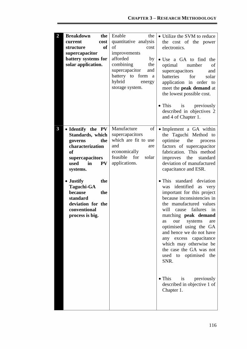
CHAPTER 3 – RESEARCH METHODOLOGY
116
2 Breakdown the
current cost
structure of
supercapacitor
battery systems for
solar application.
Enable the
quantitative analysis
of cost
improvements
afforded by
combining the
supercapacitor and
battery to form a
hybrid energy
storage system.
Utilize the SVM to reduce
the cost of the power
electronics.
Use a GA to find the
optimal number of
supercapacitors and
batteries for solar
application in order to
meet the peak demand at
the lowest possible cost.
This is previously
described in objectives 2
and 4 of Chapter 1.
3 Identify the PV
Standards, which
governs the
characterization
of
supercapacitors
used in PV
systems.
Justify the
Taguchi-GA
because the
standard
deviation for the
conventional
process is big.
Manufacture of
supercapacitors
which are fit to use
and are
economically
feasible for solar
applications.
Implement a GA within
the Taguchi Method to
optimise the process
factors of supercapacitor
fabrication. This method
improves the standard
deviation of manufactured
capacitance and ESR.
This standard deviation
was identified as very
important for this project
because inconsistencies in
the manufactured values
will cause failures in
matching peak demand
as our systems are
optimised using the GA
and hence we do not have
any excess capacitance
which may otherwise be
the case the GA was not
used to optimised the
SNR.
This is previously
described in objective 1 of
Chapter 1.

CHAPTER 3 – RESEARCH METHODOLOGY
117
4 Construct lab scale
prototype design
and fabrication
A low cost testing of
ideas and methods
previously
mentioned above.
Run system with
predictive SVM and
compare result by running
system with power
electronics.
Run both systems with
and without
supercapacitor in the
circuit.
SOC profile (100 cycles
life battery) for both
battery system, with and
without supercapacitor are
monitored and compared.
Table 15 summarizes how the methodology steps optimise the cost of
the Supercapacitor-Battery Hybrid Energy Storage system (SB-HESS).

CHAPTER 3 – RESEARCH METHODOLOGY
118
Table 15 Methodology steps that contributes to Cost Reduction
No. Methodology Steps Cost Reduction Outcome
1 Identify the
advantages of
combining the
supercapacitor and
battery in an energy
storage system.
Decelerate the rate of
damage mechanism of
battery by coupling the
supercapacitor.
This reduces the number
of replacement battery
throughout the lifespan
of the system.
Operational and
maintenance cost
for renewable
energy system
(RES) is reduced
for long run.
2 Identify the current
cost structure of
supercapacitor
battery systems for
solar application and
formulating an
appropriate
objective function.
Optimal sizing
supercapacitor-battery
hybrid energy storage
system (SB-HESS)
using Genetic Algorithm
(GA).
An optimal system
configuration of
the system is
obtained
according to user
requirement.
Therefore, sizing
excess in initial
number of
components for
the system to cater
the power burst is
avoidable,
allowing a more
feasible RES.
3 Use of the Taguchi
with a GA method
to optimise the
standard deviation
of the fabrication
process.
A robust supercapacitor
is fabricated for the SB-
HESS which reduced
spread in tolerance of
values which improve
system performance.
Consistent
supercapacitor
value is produced
for an optimised
SB-HESS.
4 Construct lab scale
prototype design
which allows low
cost method of
testing out idea
before large scale
implementation.
The energy control
system is controlled by
switches and the SVM-
load prediction system
(Support Vector
Machine).
This energy
management
system reduces
the cost of power
electronics
between the
energy
source/storage
and the load.

CHAPTER 3 – RESEARCH METHODOLOGY
119
3.1 Methodology Step 1
Identify the advantages of combining the supercapacitor and
battery in an energy storage system
This step was done to show how the supercapacitor-battery hybrid energy
storage (SB-HESS) maintains the high end of discharge voltage of the battery.
This helps prolong batteries lifetime as mentioned in the literature review
chapter. Hence, initial number of battery used is less and number of
replacement battery thourhgout the project lifetime is decreased as well.
Lead-acid batteries are often used in energy storage system for solar
application due to its low cost and wide availability [15]. System cost of a
renewable energy system (RES) often incorporates with initial cost,
replacement cost and operational/maintenance of the components. Lead-acid
batteries have a high impact on lifetime cost of stand-alone solar energy
systems [32, 15]. A higher lifetime cost means the batteries has shorter lifetime
as compared with other components in the system. Lifetime of battery is
dependent on battery C-rate (charge and discharge rate) which also subjects to
different power peak value. Economically, oversized batteries and extensive
fuel consumption (from diesel generator) should be avoided to cater the highest
peak for a short period of time. This increases the overall cost of the system.
Furthermore, RES is said to be greener if the number of batteries is minimised
as lead acid battery is heavy and filled with toxic and corrosive chemical [220,
221].
To highlight the advantages of this hybrid energy storage system
(prolong battery lifespan), an operation management for supercapacitor-battery
hybrid energy storage system (SB-HESS) in stand-alone solar application with

CHAPTER 3 – RESEARCH METHODOLOGY
120
optimised discharge strategies and knowledge on State-of-charge (SOC) and
State-of-Health (SOH) are unavoidable.
In this research, SOC of a battery is important to estimate the cycle life
before it fails to store electrical energy. In conventional system, batteries are
always operated at low SOC and are recharged with low currents to cater the
unpredictable sudden power peak. These stress factors are proven that it affects
lead-acid battery lifetime [44, 32, 23]. An operation management is
implemented based on the parameter which is said to be advantageous to save
the battery lifespan. This operation management controls the energy flow from
battery and supercapacitor to load by monitoring the voltage and current across
the battery running on a simulated load profile.
In this section, the cell voltage values for both battery alone system and
SB-HESS are shown theoretically. The cell voltage values are calculated to
design and implement this operation management.
3.1.1 System Description
Two systems are evaluated and compared in terms of state-of-charge (SOC):
1. The conventional single battery system which consists of battery alone
system. The system is often said to be infeasible due to the oversized of the
batteries. The system is designed such a way that the batteries accommodate
one power peak in the load profile when there is zero power output from the
renewable energy resources. This is not cost effective as the energy storage
system is oversized.
2. The supercapacitor-battery hybrid energy storage system (SB-HESS)
which consists of battery (behaves as a primary energy storage device) and

CHAPTER 3 – RESEARCH METHODOLOGY
121
supercapacitor (acts as an auxiliary energy storage device). The
supercapacitor caters for the entire power peaks, while battery supply an
optimal level of energy (average power demand) to avoid end deep discharge
voltage of the battery, keeping the optimal C-rate (in our strategy: discharge
rate) at a low discharge current.
In Section 4.2.3.2, SOC of the battery is monitored and plotted for both
systems mentioned above. Cycle life for a battery is the number of charge /
discharge cycles that can be accomplished during the lifetime of the device. It is
an estimation and depends upon an assumption of an average depth-of-
discharge. The load profile of battery cycle life provides a way of comparing
energy storage systems and also to prove that SB-HESS is optimal for the
power characteristics of the RES installation.
3.1.1.1 Battery individual energy storage system in RES
For this project, focus has been brought to the energy storage system in RES. In
stand-alone power supplies that utilize solar energy, the energy input fluctuates
substantially depending on climatic and meteorological conditions. As a result,
the batteries are frequently operated at low state-of-charges (SOC), are
frequently partial cycled and are recharged with low currents. This adversely
affects the lifetime of lead-acid batteries.
An impractical solution to this problem could be an oversized battery
with an early load shedding, to prevent deep SOC. Nevertheless, battery
remains a lack of full charges with this method. Stand-alone power-supply
system is incorporated with an additional controllable power supply, such as a

CHAPTER 3 – RESEARCH METHODOLOGY
122
diesel generator Figure 33 [167, 222]. With such a generator, a full charge can
be reached anytime even when the battery still has sufficient energy stored to
supply the stand-alone system. However, this causes additional fuel
consumption adding to the operational cost of the system. Utilization of diesel
generator in RES is an increase in battery lifetime. However, it reduces the
solar fraction. Solar fraction is the ratio of the amount of input energy
contributed by a solar energy system to the total input energy required for a
specific load profile. For a greener system, RES with generator is not
favourable and considered in this project. Over-increased number of batteries
which evidently spikes up the investments costs should be omitted.
Figure 33 Conventional Stand-alone renewable energy system with PV-
generator and diesel generator

CHAPTER 3 – RESEARCH METHODOLOGY
123
3.1.1.2 Supercapacitor-battery hybrid energy storage system
(SB-HESS) in RES
Two important enhancements are done to improve the conventional PV system
mentioned above by coupling supercapacitors with the batteries as follows:
1. The number of batteries is reduced, while the system still able to deliver
power peak.
2. Extend the battery life by avoiding deep discharge through high currents at a
short instant.
Certain load applications require high current for a period of time e.g.
motor starting applications; the starting current requirement can be 6-10 times
the normal operating current of the motor [15]. Normally the peak current
requirements are satisfied by the seal lead acid battery alone. The number of
sealed lead acid batteries in this situation is large in order to deal with the high
current. The peak current demand might only need to be met for a few seconds
at a particular time. Sizing the battery based on the power peak can be costly.
By utilizing supercapacitor-battery hybrid energy storage system as
shown in Figure 34 [15] , the number of battery is proven to be reduced and a
higher SOC is maintained. This is greatly due to the characteristic of the
supercapacitor and battery. Supercapacitor has a greater power density than the
battery, which allows the supercapacitor to provide more power over a short
period of time [38, 52, 53]. Conversely, the battery has a much higher energy
density compared to a supercapacitor allowing the battery to store more energy
and release it over a long period of time. In the hybrid system the peak power
requirements of the load are supplied by the supercapacitor and the seal lead

CHAPTER 3 – RESEARCH METHODOLOGY
124
acid battery supplies the lower continuous power requirements [223, 79, 76,
224].
Figure 34 Supercapacitor-Battery Hybrid Energy Storage System
(SB-HESS)
This supercapacitor-battery hybrid energy storage system solution
would be effective for applications that reside in remote sites where regular
battery maintenance is impractical or even impossible.
The supercapacitor is also a solution where ambient temperatures make
it difficult to keep batteries inside the recommended operating range without
compromising battery capacity and lifetime. SB-HESS aids in maintaining the
battery to operate at an optimal range without draining it.
Supercapacitors are safer for the environment since they contain fewer
hazardous materials compared to batteries [38]. Therefore, the lesser number of
battery is used, the greener is the system.

CHAPTER 3 – RESEARCH METHODOLOGY
125
3.1.2 Operation of SB-HESS (prototype) Management
The strategy focuses on optimising battery discharging. A quantitative
assessment of the efficiency of operation management of the proposed hybrid
energy storage system is shown below. Equation 26 shown below is used to
design an operation management system for the proposed hybrid energy storage
system. It is proven in [23, 32] that partial SOC of battery leads to strong and
partially irreversible sulphation of the battery and thus reduces the battery
lifetime. A threshold voltage of battery for the system is determined by
considering the parameters shown below. This threshold voltage value is
important to ensure the battery is individually switchable according to a
threshold voltage level that is calculated based on the desired current state-of-
charge (SOC), depth-of-discharge (DOD) and other parameters data set of the
lead acid battery. This operation management system reduces time for battery to
remain at low SOC, a decrease in the battery current rate, and hence full
chargers during normal operating condition (steady-state).
This model describes the current-voltage characteristic of the lead-acid
battery. It is reported in [32], it has an average accuracy for currents typically
applied in stand-alone system for better than 2%. The required parameters used
in the equations were already determined on the basis of experimental data in
[32]. It is regardless of the physical significance of each parameter, which
results from derivation, a theoretical calculation of the parameters is not
possible. A second set of parameters reported in [3] has extended in the
charging process. The terminal voltage of a battery has an additive composition
consisting of open-circuit value, which approximately is in proportion to the

CHAPTER 3 – RESEARCH METHODOLOGY
126
acid density and thus to the SOC, as well as the reaction, diffusion,
crystallization and resistance over-voltages. These over-voltages are taken in
the individual terms in Shepherd Model as a basis [23].
The concentration of the electrolyte changes as part of the chemical
processes that take place when the battery is charged and discharged. During
repeated cycles a concentration gradient can build up (from top to bottom) and
the battery then behaves as several batteries of different concentrations working
in parallel. Consequently, the charge acceptance is reduced and the capacity
deteriorates. Eventually, the concentration gradients are levelled through
diffusion. However, this takes a long time. They can be quickly removed by
periods of gassing, where the rising bubbles effectively mix the electrolyte
resulting in a more homogeneous electrolyte [23]. Hence, diffusion processes
based on concentration gradients are not taken into consideration. Another term
of the Shepherd Model [23, 32], which describes the crystallization
overvoltage, is disregarded as well.
The formulation used in the model (Equation 26 [23]) consists of four
terms:
( ) ( ) ( ) ( )
( )
( )
( )
( )
Equation 26

CHAPTER 3 – RESEARCH METHODOLOGY
127
Table 16 Terms and Explanation for Equation 26
Terms Explanation [32]
Open-circuit voltage,
Uo =
Full discharge equilibrium voltage i.e. the
voltage of the cell when it is fully
discharged and rested long enough for the
electrolyte to reach constant density.
( ) This term is associated with the state of
charge (SOC) of the battery. It is
assumed that this term is linear with
respect to the depth of discharge (DOD).
( ) ( )
Ohmic losses in the battery through the
use of the internal resistance, which is an
aggregate value of the various loss
mechanisms which are proportional to the
current. The major factors are the grid
resistance and the resistance of the
electrolyte.
( )
( )
( )
( )
The last term in the equation shows the
reaction over-voltages. M represents the
transfer overvoltage coefficient. It
models the charge factor over voltage and
is significant when the battery is very
close to being empty or full.
However, several terms are neglected including dynamic terms to model
the electrolyte diffusion and the dependence of the resistive elements to the
SOC. This is unproblematic. The dynamic behavior of batteries is not relevant
UOd

CHAPTER 3 – RESEARCH METHODOLOGY
128
in this context and the dependence of the resistive elements on SOC is both
small and, as far as a parameter fit for determining the constants is concerned, is
taken into account by the fourth term.
Table 17 shows the parameter data set [23] for batteries which was used
for the Equations 3 above.
Table 17 Parameter data set for batteries
Terms (Units) Charge, c Discharge, d Description index
UOi (V) 2.26 2.1 Equilibrium voltage
gi (VAh-1) 0.13071 0.09654 Electrolyte coefficient
ρi (ohm-cm) 0.43609 0.37885 Internal resistance
Mi 0.36488 0.28957 Transfer overvoltage coefficient
Ci 1.001 1.642 Capacity coefficient
where i = c or d.
Two energy storage systems are examined and compared, which are
battery-individual energy storage system and supercapacitor-battery hybrid
energy storage system theoretically. In conjunction with that, the Ibatt and the
DOD varies in different cases. At peak demand, battery individual energy
storage system and battery supercapacitor hybrid energy storage system show
different values for battery voltage and current ( and ). According
to the equation shown below, two different cell voltages are compared in two
different operating conditions. It is assumed that:
1. A same type of sealed-lead-acid battery is used.
2. Both systems are applied on the same load profile generated by a 3A
programmable load for a lab scale prototype system.
Ucell (t) Ibatt (t)

CHAPTER 3 – RESEARCH METHODOLOGY
129
Figure 35 Simulated Load Profile
3. The critical situation is to be considered (night or rainy day) where only
energy storage system is supplying to the peak load demand.
4. When the cell is discharging, for all (Ibattt) ≤ 0
Table 18 Theoretical Ucell (V) and Ubatt(V) Battery
Systems Ibatt (A) DOD
(%)
Ucell (V) Ubatt(V)
Battery Individual
System
2.5 80 1.99 11.99
Supercapacitor/Battery
hybrid system
1.5 20 2.06 12.41
Theoretically speaking, the Ibatt value is taken from the load_profile 1
which is presented in Figure 35 above. Battery individual system suffers high
current peak (2.5A) as the batteries cater for the entire power peak. However,
batteries are not stressed up for the power peak in the hybrid energy storage
system with the presence of supercapacitor.
The battery stand-alone system suffers a longer period of low SOC
cycle. It means that the battery individual system remains for an extended
period in a partial SOC, which leads to sulphation within battery and thus
reduces the battery lifetime [76, 45]. Partial state of charge means the cycling
has an inherent advantage in that, within a fairly broad SOC window of

CHAPTER 3 – RESEARCH METHODOLOGY
130
approximately 20% - 80%, the battery is neither deep discharged nor put into
overcharge under normal conditions of charge and discharge. This is not a good
approach as only a fraction of the available energy is delivered on each cycle.
Hence, the DOD is always higher for the conventional system to cater the
power peak.
3.1.3 Summary
Theoretically proven that the operating cell voltage is lower for the
battery individual energy storage system. This shows that the battery is
drained to supply the high current peak and the battery is approaching
lower end-discharge-voltage. This shortens battery life as the battery is
deep discharging high rates for short periods.
By coupling supercapacitor and battery in an energy storage system, it
maintains high SOC of the battery and avoids low DOD. It certainly
reduces the rate of damage mechanism of batteries.
Ibatt is lower in hybrid energy storage system as the battery is not
required to supply power peak in the load profile. Hence, the number of
battery (overall capacity of battery) is reduced.
Values of desired DOD, desired SOC and Ubatt (V) set as a guideline to
design an energy control strategy which is presented in Methodology
Steps 2.
The role of supercapacitor in a hybrid energy storage system is to meet
peak load demand and also allows for the downsizing number of
battery, reducing the depth-of-discharge (DOD), reducing the sulphation
of battery, and most importantly, prolongs the battery’s lifespan.

CHAPTER 3 – RESEARCH METHODOLOGY
131
3.2 Methodology Step 2
Identify the current cost structure of supercapacitor battery
systems for solar application
In the previous section, it explains how the presented advantages of pairing
supercapacitor to the battery system extends battery lifespan. In this section,
design, simulation and optimisation on the hybrid energy storage system are
carried out using HOMER and GA. The rationale shown below motivates the
design, simulation and cost optimisation on the hybrid energy storage system:
1. Maintain an optimal level of SOC battery during discharge.
2. Avoid low sudden DOD.
3. Avoid end-of-discharge voltage suggested in the data sheet before the
battery has to be recharged.
Optimal sizing PV-Wind-Battery system using a GA and HOMER are
carried out in this section. HOMER covers energy storage devices other than
lead acid batteries such as flywheels, hydrogen and flow batteries. However,
supercapacitor is not incorporated in HOMER library. Designing and
optimising system with supercapacitor is merely impossible in HOMER. The
idea has been presented using the GA to optimal size the autonomous SB-HESS
due to the flexibility of the GA in coding a large number of components. The
implemented GA fitness functions embeds with the essential information which
is related to initial, maintenance and operational cost of the components used in
the systems based on the market price. The conventional battery alone system
and SB-HESS are designed and optimised for 20 years. 20 years is selected
based on the longest lifespan components in the system for this simulation and
optimization, which is PV panel [123]. According to [123], PV panel can last

CHAPTER 3 – RESEARCH METHODOLOGY
132
approximately 20 – 25 years of lifespan, but the efficiency drops after 12 years
installation and it is estimated from 90% to 85%-80%. It applies in HOMER
component input and GA fitness function.
In the sub-sections below, methodology steps on:
1. optimal sizing PV-wind-battery system using HOMER
2. optimal sizing PV-wind-battery system using GA, and
3. optimal sizing PV-battery-supercapacitor system using GA are shown
3.2.1 Design, Simulation and optimization of PV-wind-battery
system using HOMER
HOMER, Micropower Optimization Model is a computer model developed by
the U.S National Renewable Energy Laboratory (NREL) to assist in the design
of micropower systems and to facilitate the comparison of power generation
technologies across a wide range of applications [14]. Generally, HOMER
models a power system’s physical behaviour and its life-cycle cost, which is the
total cost of installing and operating the system over life span. This also means,
in the simulation process, it models a particular system configuration; the
optimization process determines the best possible optimal system configuration
which satisfies the user-specified constraints at the lowest total net present cost
(NPC) [225] .
In this project, HOMER was used to validate the efficacy of the GA and
its objective function where this is proven approximately the same GA was
used for the prototype system.

CHAPTER 3 – RESEARCH METHODOLOGY
133
3.2.1.1 Design and Simulation of RES
i. System Description
A PV-Wind-battery system is designed and simulated using HOMER. The
specification of the components used is described in the section below. This
design of renewable energy system consists of hybrid energy sources that is
coupled with batteries only system. Diesel generator is not considered in the
system. This is to ensure a zero CO2 emission system. The simulation result
obtained in paper [146, 226] shows that the power system with PV-Diesel
generator-Battery has a lower installation cost, but higher operation and
maintenance costs; additionally, it was less efficient and released contaminating
emissions (such as CO2, NOx and particles). Diesel generator is not taken into
consideration for this project. The reason being is to guarantee zero emission of
hazard gas and a greener system. Hence, PV-Wind-Battery is designed and
simulated using HOMER.
1. Location
In this study, hypothetical model a household in a residential area in the
geographical coordinate of the location Semenyih is
Latitude: 2.9° N,
Longitude: 101°53 E,
Altitude: 39 m (approximately) above sea levels

CHAPTER 3 – RESEARCH METHODOLOGY
134
Figure 36 Location for the hypothecial model
Figure above is extracted from Google Earth [227].
2. Electrical Load Profile
Deciding the load profile is important to design PV-Wind-Battery system
because an optimised design of RES is always catered for a specific load
profile. Oversized of energy sources are infeasible and cost ineffective. Load
profile is simulated based on the electrical appliances power rating shown in
Table 19.
Figure 37 Load Profile from HOMER
Coordinate: 2°9N longitude, 101°53E
latitude
Address: Semenyih, 43000 Selangor.

CHAPTER 3 – RESEARCH METHODOLOGY
135
HOMER simulates the operation of a system by making energy balance
calculations for each of the 8760h in a year. Measured hourly load profiles are
not available, so load data were synthesized by specifying typical daily load
profiles and then adding some randomness of daily 10% and hourly 15% noise.
These have scaled up the annual peak load to 1.5 kW and primary load to 5.4
kWh per day.
Figure 38 HOMER implementation of PV-Wind-Battery Energy System
Table 19 Energy demands of the electrical appliances
Electrical Appliances Power (W)
Compact Fluorescent Bulb 15
Refrigerator 700
Personal Computers 600
Control System/Electrical Power Point 500
Fans 150
Washing Machine 300

CHAPTER 3 – RESEARCH METHODOLOGY
136
3. Renewable Energy Sources
Solar Energy
HOMER synthesizes solar radiation values for each of the 8760h of the
year by using Graham algorithm [228, 229]. This algorithm produces
realistic hourly data, and it is easy to use because it requires only the
geographical coordinates and the monthly average solar data values. The
synthetic data displays realistic day-to-day and hour-to-hour pattern. The
synthetic data are created with certain statistical properties that reflect
global average values. Result obtained in [228] show that synthetic solar
data produced virtually the same simulation results as real data as the
result obtained in [229].
Solar radiation data for the selected region was obtained from the
NASA Surface Meteorology and Solar Energy website (NREL) [156,
230]. The solar radiation data and the clearness index for the selected site
mentioned above is shown below in Table 20 and Figure 39. The solar
irradiance data shown is the monthly average data for year 2012 at the
longtitude and latitude mentioned above.

CHAPTER 3 – RESEARCH METHODOLOGY
137
Table 20 Baseline Data for PV
Scaled Annual Average( kWh/m2/day): 4.12
Figure 39 Average monthly solar radiation kWh/m2/day and clearness
index
Month Clearness Index Daily Radiation
(kWh/m2/day)
January 0.458 4.505
February 0.481 4.918
March 0.489 5.126
April 0.488 5.023
May 0.474 4.669
June 0.496 4.733
July 0.485 4.671
August 0.497 4.994
September 0.475 4.912
October 0.483 4.944
November 0.477 4.709
December 0.481 4.488
Average: 0.481 4.806

CHAPTER 3 – RESEARCH METHODOLOGY
138
The clearness index has a simple definition. It is equal to the global solar
radiation on the surface of the earth divided by the extra-terrestrial
radiation at the top of the atmosphere. In other words, it is the proportion
of the extra-terrestrial solar radiation that makes it through to the surface
[231, 232]. It varies from around 0.8 in the clearest conditions to near
zero in overcast conditions. The monthly average clearness index may
vary from near 0.8 down to maybe 0.2 surface [231].
One can calculate precisely the amount of solar radiation that
strikes the top of the atmosphere anywhere on earth with just the latitude.
Therefore, if the amount of radiation striking the surface is specified,
HOMER immediately divides that value by the amount of radiation
striking the top of the atmosphere to calculate the clearness index [233].
If the clearness index is specified instead, HOMER multiplies that value
by the extra-terrestrial radiation to calculate the amount of radiation
striking the surface.
In this case, the average of the clearness index and daily radiation
are 0.481 and 4.806 respectively. The value of clearness index and daily
radiation do not fluctuate much. From Table 20, it tells us that the
guaranteed annual power is 4.12 kWh/m2/day which is good for solar
energy system.
Wind Energy
Since the energy from the PV array is not sufficient to supply the average
daily energy demand, wind turbine is one of the supporting combined

CHAPTER 3 – RESEARCH METHODOLOGY
139
alternative to provide the remaining power needed to charge up the
battery and load demand. Scaled annual average shown in the Table 21 is
used to determine the sensitivity analysis in HOMER simulation. This
also implies that the annual guaranteed wind speed is 2.89m/s. HOMER
determines a scaling factor by dividing the scaled annual average by the
baseline annual average and multiplies each baseline value by this factor.
By default, HOMER sets the scaled average equal to the baseline average,
which results in a scaling factor of 0.95. This scaled annual average
examines the effect of higher or lower wind speeds on the feasibility of
system designs.
Table 21 Baseline Data for wind speed
Month Wind Speed (m/s)
January 1.800
February 1.800
March 3.000
April 3.000
May 3.000
June 3.000
July 4.000
August 5.000
September 5.000
October 3.000
November 2.000
December 1.800
Average: 3.041
Scaled Annual Average (m/s): 2.89
In [161, 228] say that as the wind turbine tower is higher, it
increases the initial, operational and maintenance cost, however the
wind speed is tends to be higher at higher position. An anemometer
height is one of the parameter in HOMER simulations.

CHAPTER 3 – RESEARCH METHODOLOGY
140
When hourly wind speed data is not available, hourly data can be
generated synthetically from the monthly averages. HOMER's synthetic
wind speed data generator is different to use than the solar data because it
requires four parameters [157, 229].
i. The Weibull (k) value: k value is a measure of distribution of wind
speed over the year. The default value is 2 because this has been
shown to represent most wind regimes fairly accurately. The default
value is used in this study.
ii. The autocorrelation factor: this factor measures the randomness of
the wind. Higher values indicate that the wind speed in 1h tends to
depend strongly on the wind speed in the previous hour. Lower
values mean that the wind speed tends to fluctuate in a more random
fashion from hour-to-hour. The autocorrelation factors tend to be
lower (0.70−0.80) in areas of complex topography and higher
(0.90−0.97) in areas of more uniform topography. In this study, 0.85
is used. 0.85 is the default value and is the mid-value of the higher
and lower value.
iii. The diurnal pattern strength: it is a measure of how strongly the wind
speed depends on the time of day. In most locations, the afternoon
trends to be windier than the morning. A high value of the diurnal
pattern strength shows that there is a relatively strong dependence on
the time of day and vice versa [234, 235]. In this study, 0.25 is used.
iv. The hour of peak wind speed: it is the time of day that tends to be
windiest on average throughout the year. In this study, 15:00 is used

CHAPTER 3 – RESEARCH METHODOLOGY
141
as the hour of peak wind speed according to the simulated wind
speed in HOMER. Table 22 shows advanced parameters for HOMER
wind resource input.
Table 22 Advanced parameters for HOMER wind resource input
Parameter Unit
Weibull (k) value 2
autocorrelation factor 0.85
diurnal pattern strength 0.25
hour of peak wind speed 15:00
The parameters shown in Table 22 are taken from [234, 235] .
Based on the studies carried out in [234, 235], these values are said to be
optimal values in order to obtain high wind energy.
4. Economics
Considering the project lifetime to be 20-years, the annual real interest was
taken as 0%. Generally speaking, the real interest rate is equal to the nominal
interest rate minus the inflation rate. The appropriate value for this variable
depends on current macroeconomic condition, the financial strength of the
implementing entity, and concessional financing or other policy incentives
[236, 156]. However, in this case, annual real interest is not our concern as
Malaysia government subsidises the renewable energy system. The capacity
shortage fraction (C.S.F) is the fraction of the total load plus operating
reserve that system fails to supply. For this HOMER’s simulation part, C.S.F
of 0%, 0.01% and 0.02% are simulated.

CHAPTER 3 – RESEARCH METHODOLOGY
142
5. Photovoltaic panels
HOMER deals with PV array in terms of rated kW, not in m2. HOMER
assumes that the output of the PV array is linearly proportional to the
incident solar radiation. The PV modules composed of several solar cells are
clustered in series–parallel arrangement to form solar arrays with the
necessary capacity. In the proposed systems, PV array sizes taken into
account were 0 (no PV array), 2, 4, 6, 8, 10, 12, 14, 16, 18 and 20 kW.
The parameters considered for the simulation of solar PV panels are
tabulated in Table 23. Efficiency of solar panels drops as the temperature of
the solar panels increase. It is worth mentioning that HOMER's PV input
GUI has a derating factor. Ought to be the slightly hotter climate according
to [233] a derating factor of 80% was applied to the electric production from
each panels instead of the default value of 90%. The purpose of ‘derating
factor’ is to compensate the reduction in efficiency of the PV panels as in the
actual conditions are less favourable than standard test conditions STC, (cell
temperature = 25°C and solar irradiance = 1 kW/m2, provided by the
manufacturer, as well as the ambient temperature and irradiation conditions)
[176]. This derating factor reduces the PV power production by 20% to
approximate the varying effects of temperature, dust and wiring losses on the
panels. The PV panels were modelled as fixed and tilted south at an angle
equal to latitude of the location.
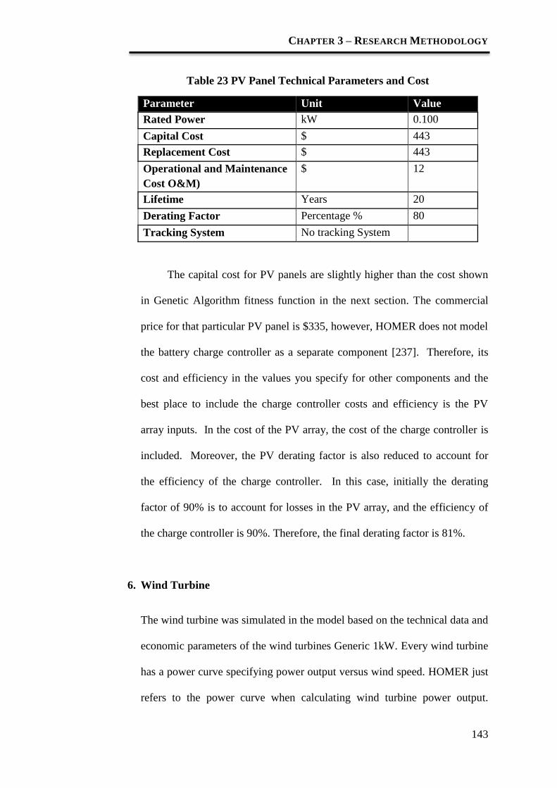
CHAPTER 3 – RESEARCH METHODOLOGY
143
Table 23 PV Panel Technical Parameters and Cost
Parameter Unit Value
Rated Power kW 0.100
Capital Cost $ 443
Replacement Cost $ 443
Operational and Maintenance
Cost O&M)
$ 12
Lifetime Years 20
Derating Factor Percentage % 80
Tracking System No tracking System
The capital cost for PV panels are slightly higher than the cost shown
in Genetic Algorithm fitness function in the next section. The commercial
price for that particular PV panel is $335, however, HOMER does not model
the battery charge controller as a separate component [237]. Therefore, its
cost and efficiency in the values you specify for other components and the
best place to include the charge controller costs and efficiency is the PV
array inputs. In the cost of the PV array, the cost of the charge controller is
included. Moreover, the PV derating factor is also reduced to account for
the efficiency of the charge controller. In this case, initially the derating
factor of 90% is to account for losses in the PV array, and the efficiency of
the charge controller is 90%. Therefore, the final derating factor is 81%.
6. Wind Turbine
The wind turbine was simulated in the model based on the technical data and
economic parameters of the wind turbines Generic 1kW. Every wind turbine
has a power curve specifying power output versus wind speed. HOMER just
refers to the power curve when calculating wind turbine power output.

CHAPTER 3 – RESEARCH METHODOLOGY
144
Technical and economic parameters for selected wind turbine are tabulated
in Table 24.
Table 24 Wind Turbine-Technical Parameters and Cost
Parameter Unit Value
Rated Power kW 1
Capital Cost $ 2240
Replacement Cost $ 2240
Operational and Maintenance Cost (O&M) $ 118
Lifetime Years 20
Hub Height m 15
7. Converters (Inverter)
A power converter is used to maintain the flow of energy between the AC
and DC components. Table 25 shows the technical and economic parameters
of the converter. The inverter and rectifier efficiencies were assumed to be
85% and 90% for the sizes of 2, 4, 5, 6, 7, 8, 9, 10, 12, 14, 16 kW
considered. The sizes are defined for the purpose of providing a search space
in HOMER simulation. HOMER also simulates each system with power
switched between the inverter and the generator. These devices were not
allowed to operate in parallel.
Table 25 Converter-Technical Parameters and Cost
Parameter Unit Value
Rated Power kW 1.5
Capital Cost $ 1942
Replacement Cost $ 1942
Operational and Maintenance
Cost (O&M)
$ 19
Lifetime Years 20

CHAPTER 3 – RESEARCH METHODOLOGY
145
8. Batteries
HOMER allows user to add new component with the new specification and
cost of the battery. A Hoppecke 12V, 120Ah batteries are used in this PV-
Wind-Battery system. The specifications are shown in Table 26. According
Hoppecke data sheet [238], the minimum battery life is 10 years if the
battery is not drained more than DOD 80-90% for ~600 cycles at an optimal
temperature. Battery lifetime greatly depends on the pattern of the load
profile.
HOMER uses the Kinetic Battery Model and represents batteries as a
‘two tank’ system [239]. One tank provides immediately available capacity
while the second can only be discharged at a limited rate.
HOMER set the DC bus voltage by defining a number of batteries per
string. This defines the number of battery connects in series. On the battery
input page, the number of batteries per string is specified. HOMER displays
the bus voltage, which it calculates by multiplying the battery's nominal
voltage by the number of batteries per string.
Table 26 Specification of Hoppcake Battery
Parameter Unit Value
Nominal Voltage Volt 12
Nominal Capacity Ah (kwh) 118 (1.42)
Maximum Charge Current A 60
Round-trip efficiency Percentage (%) 82.46
Maximum State-of-Charge Percentage (%) 80
Capital Cost $ 316
Operational and
Maintenance Cost O&M)
$ 6.32
Replacement Cost $ 316

CHAPTER 3 – RESEARCH METHODOLOGY
146
ii. Control Strategy
Control strategy used in HOMER simulation is charge-following. The set
point of battery SOC is set to 0.8. After modelling is done, the model will be
implement based on the parameters, constraint and the output obtained from
HOMER.
In hybrid source systems with batteries and without diesel generators, the
dispatch strategy is simple where the battery charges if the renewable energy is
in excess after meeting the demand, and the battery discharges if the load
exceeds the renewable energy.
3.2.1.2 Summary
HOMER uses constraint to optimise the cost of the system. Stating the
different constraints in HOMER leads to different optimization result.
For example, the capacity shortage of the system is a constraint in
HOMER.
Cost and technical specification of components are defined in HOMER
before the simulation and optimization result is obtained. This is
important to ensure a feasible simulation.
Simulation is the first step of implementing a prototype. This is
important to save unnecessary cost in implementing a system.
The result obtained in HOMER for the PV-Wind-Battery is compared
with the result obtained from the implemented GA fitness functions
shown in the next section.

CHAPTER 3 – RESEARCH METHODOLOGY
147
3.2.2 Methodology Optimal Sizing of RES using the GA
Supercapacitor is the auxiliary energy storage in the implemented renewable
energy system (RES). Design and simulation for the implemented RES cannot
be done in HOMER as the HOMER library does not include supercapacitor.
However, if model a large supercapacitor that functions as an energy storage
device, this means that the system can use it to store energy from one time step
to the next or from one day to another, it can be done that using HOMER's
battery module. A flat capacity curve, a really high lifetime throughput, and a
high round-trip efficiency for a supercapacitor are expected. On the other hand,
if the supercapacitor does not store much energy and it is sufficient to serve the
load for a few seconds, this primarily affects power quality or system stability.
HOMER does not allow to model that because it does not model those effects
as this is using the battery module theory. Therefore, it is not feasible to
optimise the implemented system using HOMER.
GA is chosen for the optimal sizing the implemented RES as GA is not
easy to trap in local optimal point and a higher freedom in coding more
parameters as compared to other optimization techniques mentioned in Section
2.2.2. The proposed stand-alone system includes hybrid energy storage which
consists of batteries and supercapacitors. This system is compared with the
battery only RES. By considering the 20-year round total system cost, the
objective function is made up of the sum of the respective components initial
capital, maintenance and operational costs. Concept on constructing fitness
functions which subjects to constraints is shown to optimise PV-wind-battery
system, PV-wind-battery-supercapacitor system and a prototype PV-battery-
supercapacitor are presented in Section 3.2.2-1, Section 3.2.2-2 and Section

CHAPTER 3 – RESEARCH METHODOLOGY
148
3.2.2-3 accordingly. These GA fitness functions are computed to the GA code
written using MATLAB R2011b. The code is documented in Appendix A2.
3.2.2.1 Optimal Sizing of Battery Single Energy Storage System
(SB-HESS) using the GA
The objective function is the total net present cost (NPC) of the system which
also represents the life-cycle cost. Net present cost includes the initial cost of
the components, and all the future cost which consists of the maintenance and
operational cost of the components throughout the total life of installation. The
maintenance and operation cost of each unit of the components per year has
been set to 2% of the corresponding capital cost. Normally, the life span of the
system follows the life span of the solar panels [123, 240] . This is because the
life span of solar panel in the system has the longest life span among the other
components [123, 240, 169]. A same location mentioned in the previous part is
used for GA optimal sizing RES, which is Semenyih. The objective function
optimises the following costs:
Cost of purchasing solar panels, wind turbines, the batteries, the
inverter, the PV battery chargers.
Cost of maintenance and operational of the solar panels, wind turbines,
the batteries, the PV battery chargers and the inverters.
Cost of replacing the batteries, the PV battery chargers, and the
inverters.
Based on the different type of cost listed above, fitness function and
constraints are constructed to design and optimise the renewable energy system.

CHAPTER 3 – RESEARCH METHODOLOGY
149
1. Fitness Function
i. PV-wind-battery system
( ) ( ) (
) ( ( ) )
( ) ( ) ( )
( ) Equation 27
where h is the height of the WG tower in meter, CPV , CWG , and CBAT are the
capital cost ($) of one module, WG and battery respectively, Ch is the capital
cost ($) for the WG tower per meter ($/m), Chm is the maintenance cost per
meter and year ($/meter/year), CCH is the capital cost of one PV battery charger
($), yCH and yINV are the expected numbers of PV battery charger and DC/AC
inverter replacements during the 20-year system lifetime (and it is equal to the
lifetime 20 years) divided by the Mean Time Between Failures (MTBF) of
power electronic converters [176, 241], CINV is the capital cost of the DC/AC
inverter, ($). Project lifetime, yp is 20 years. R is the expected number of battery
replacement which depends on ybatt. ybatt is the expected battery lifespan during
the 20-years system operation. It depends on the battery energy each hour of the
simulation by dividing the total year-to-date of charging the battery bank by the
total year-to-date amount of energy put into the battery bank. It is computed
using Equation 28 shown below:
Equation 28

CHAPTER 3 – RESEARCH METHODOLOGY
150
MCH and MINV are the maintenance costs per year ($/year) of one PV battery
charger and DC/AC inverter respectively. In addition, the number of PV battery
chargers, NCH is equal to the total number of PV power generation blocks which
depends on the number of PV modules, NPV. It is calculated using the equation
below:
Where lifetime throughput for a single battery, and
annual throughput of the a single battery, are shown
in Equation 29 and Equation 30.
Equation 29
Equation 30
, the number of batteries,
, Depth-of-discharge of the battery (where the state-of-
charge minimum SOC of the battery is set). Simulation is
carried out for, DOD = 1.0, 0.9, 0.8, 0.7, 0.6 and 0.5.
, the number of charge and discharge cycle of the
battery (based on data sheet of the battery),
, the nominal voltage of the battery,
, the nominal capacity of the battery,
, the round-trip energy efficiency, ,

CHAPTER 3 – RESEARCH METHODOLOGY
151
where is the power rating of the selected battery charger
(W) and is the maximum power of one solar panel under
standard test condition (W), under the manufacturers’
specification. In this case, the power rating for solar panel,
is 100 W and the power rating for PV battery charger, is
300 W.
Equation 31
ii. PV-battery system
Equation 32 shows the fitness function for PV-Battery system. Wind generator
terms in Equation 27 is removed and Equation 32 is formulated as follows:
( ) ( )
( ( ) )
( )
( ) ( )
( )
where
CPV and CBAT are the capital cost ($) of one module and
battery respectively,
CCH is the capital cost of one PV battery charger ($),
yCH and yINV are the expected numbers of PV battery charger
and DC/AC inverter replacements during the 20-year system
lifetime and it is equal to the lifetime 20 years) divided by
the Mean Time Between Failures (MTBF) of power
electronic converters Holtz et al., 1994),
Equation 32

CHAPTER 3 – RESEARCH METHODOLOGY
152
CINV is the capital cost of the DC/AC inverter, ($), R is the
battery lifetime.
Project lifetime, yp is 20 years.
R is the expected number of battery replacement which
depends on ybatt. ybatt is the expected battery lifespan during
the 20-years system operation. It is computed using the
Equation 28.
MCH and MINV are the maintenance costs per year ($/year) of
one PV battery charger and DC/AC inverter respectively.
2. Boundary
The fitness function for the battery alone RES is subject to the initial boundary
as shown below:
The total power of PV, Ppv and wind generator, Pwind is not more than
2.0 kW. This is defined based on the random variability (percentage) set for the
simulated load profile which is explained in the section below. For the
operaitng reserve (in this case battery) the maximum throughput for one battery
is 1.416 kWh based on the data specification of the battery. This throughput of
the battery is constrained based on the DOD defined in the system. The battery
is sized based on the highest peak in the load profile for the battery-only

CHAPTER 3 – RESEARCH METHODOLOGY
153
system. It also depends on the loss of power supply probability (LPSP) set by
the user. It is a trade-off between the system cost and the power failure time.
The concept of the LPSP is explained in the section below.
3. Constraints
Constraints in a GA are important because it places the objective function in the
proper search space which is related to real life conditions in which we wish to
optimise the system. With proper constraints we are able to solve the objective
function accurately and implement that solution in the practical situation under
consideration. GA searches thoroughly over the search space. With improper
constraints the GA will still find the optimal solution, however, it may not be
practical to implement.
In order to optimise the cost of a renewable energy system, a
compromise must be achieved between the size of the energy storage system
and the power requirement. There are three constraints used for the
implemented fitness functions.
i. Loss of Power Supple Probability (LPSP)
LPSP is defined as the probability that an insufficient power supply results
(when the hybrid system PV array, wind turbine and battery storage) is unable
to satisfy the load demand [48]. It is a feasible measure of the system
performance for an assumed or known load distribution. A LPSP of 0 means
the load will always be satisfied; and an LPSP of 1 means that the load will
never be satisfied [48]. LPSP is a statistical parameter [242, 243]; its
calculation is not only focused on the abundant or bad resource period.

CHAPTER 3 – RESEARCH METHODOLOGY
154
Therefore, if renewable energy output is low, the system suffers from a higher
probability of losing power. This is because of the intermittent solar radiation
and wind speed characteristics, which highly influence the resulting energy
production, power reliability analysis has been considered as an important step
in any system design process. A reliable electrical power system means a
system has sufficient power to supply the load demand during a certain period
or it also means that it has a small LPSP [244].
Considering the energy accumulation effect of the battery, to present the
system working conditions more precisely, the chronological method is
employed in this research. The LPSP from time 0 to T can be expressed as
follows,
∑
∑( ( ) )
Equation 33
where T is the number of hours in this study with hourly weather data input.
From the load profile shown in Figure 40, T = 24. The power failure time is
defined as the time that the load is not satisfied when the power generated by
both the wind turbine and the PV array is insufficient and the storage is
depleted battery SOC falls below the allowed value (and
still has not recovered to the reconnection point).
As mentioned previously, there is trade-off between system cost and the
power reliability. If the user willing to pay for a 0 LPSP system, the system cost

CHAPTER 3 – RESEARCH METHODOLOGY
155
is higher and hence, the available power, is always more than
.
For example, if
. This tells us that there is no downtime
for this system every single peak of the load profile is covered even the highest
peak (1000W as shown in Figure 40). Simulation is done for 0, 0.01, 0.02 LPSP
systems and result obtained is presented in Section 4.2.2.
Figure 40 Load profile
The same load profile in HOMER was used for GA optimal sizing RES shown
in Figure 40. From the figure above, the highest load peak is 1000W.
ii. Constraint for power from Renewable Energy Sources
Constraint for renewable energy sources is clear. The total power
generated from PV panel and wind generator are not more than 2.0kW for a 0
(zero) LPSP. As mentioned earlier, a random variability of 10% of day-to-day
and 20% time-step-to-time-step are added to the total power needed from the
renewable energy sources. The efficiency of the PV panel and wind generator
0
200
400
600
800
1000
1200
1 2 3 4 5 6 7 8 9 10 11 12 13 14 15 16 17 18 19 20 21 22 23 24
PO
WE
R (
kW
)
Number of Hours
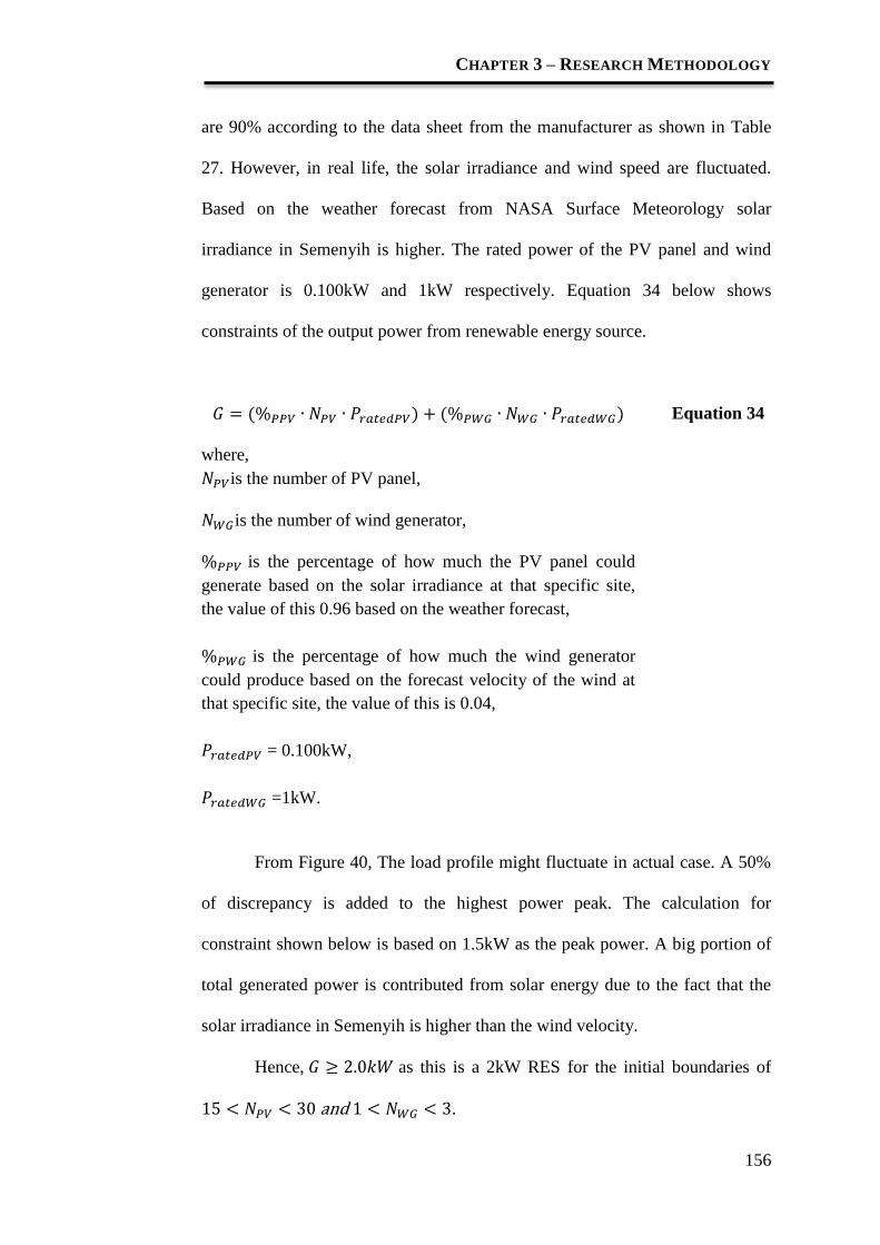
CHAPTER 3 – RESEARCH METHODOLOGY
156
are 90% according to the data sheet from the manufacturer as shown in Table
27. However, in real life, the solar irradiance and wind speed are fluctuated.
Based on the weather forecast from NASA Surface Meteorology solar
irradiance in Semenyih is higher. The rated power of the PV panel and wind
generator is 0.100kW and 1kW respectively. Equation 34 below shows
constraints of the output power from renewable energy source.
( ) ( ) Equation 34
where,
is the number of PV panel,
is the number of wind generator,
is the percentage of how much the PV panel could
generate based on the solar irradiance at that specific site,
the value of this 0.96 based on the weather forecast,
is the percentage of how much the wind generator
could produce based on the forecast velocity of the wind at
that specific site, the value of this is 0.04,
= 0.100kW,
=1kW.
From Figure 40, The load profile might fluctuate in actual case. A 50%
of discrepancy is added to the highest power peak. The calculation for
constraint shown below is based on 1.5kW as the peak power. A big portion of
total generated power is contributed from solar energy due to the fact that the
solar irradiance in Semenyih is higher than the wind velocity.
Hence, as this is a 2kW RES for the initial boundaries of
and .

CHAPTER 3 – RESEARCH METHODOLOGY
157
iii. Constraint for battery connection
DC bus voltage is 48V. This is important to decide the number of battery in one
string. This also means that how many batteries are connected in series based
on the battery specification. Hopecake battery 12V, capacity of 118Ah and
throughput of 1.416kW is used in this study. The minimum is 4 (
) due to the DC bus voltage of the system.
iv. Constraint for Autonomy
A, autonomy of the system constraints the number of batteries used with
different LPSP value. This is an autonomous system, operating reserve (battery
in this case) plays an important role in the system and it has a big impact on the
net present cost of the system to maintain a zero load rejection (0% LPSP).
Different value of depth-of-discharge (DOD) are applied to the simulation.
Total usable battery capacity is optimised to cater power, PA. From Figure 40,
the highest peak is 1kW, PA is 1kW as battery is sized based on the highest peak
for the battery-only system.
A is an inequality constraint where A, is the autonomy for the batteries
in hours. The constant value of A is set by the user depends on the LPSP. If 0
LPSP, A is always more than 24 hours to avoid zero downtime. Equation 35
shown below is used to construct autonomy. For night, when wind speed is very
low and no solar irradiance (the renewable energy source is nearly absent),
operating reserve (battery in this case) plays an important role to ensure zero
load rejection output. A of the system is assigned as follows:

CHAPTER 3 – RESEARCH METHODOLOGY
158
where
is the number of batteries,
is the nominal voltage of the battery, 12V
is the nominal capacity of the battery, 118Ah
is Depth-of-discharge of the battery (where the
minimum SOC of the battery is set).
is the power that battery is required to cater when there
is zero output renewable power. It is also based on the
load profile. For a battery alone system, is 1kW. The
highest peak in the load profile is supplied by the battery
only.
Equation 35
Equation 36

CHAPTER 3 – RESEARCH METHODOLOGY
159
3.2.2.2 Optimal Sizing of Supercapacitor-Battery Hybrid energy
storage system (SB-HESS) using the GA
This methodology aims to minimise the 20-year round total system cost
function (Zx) by taking the total capital of the devices (Cc), the costs of the 20
years round maintenance (Cm). The set of variables (x) that consists of umber of
PV modules (NPV), WG (NWG), batteries (NBAT), supercapacitor (NSCAP) battery
chargers (NCH), PV charges, and the height (h) of the installation of the wind
generator is optimised. The focus of the objective function is the number of
replacement batteries which is based on the battery lifespan, R and the number
of batteries NBAT that benefits from the inclusion supercapacitor NSCAP in the
energy storage system. The total system cost function is equal to the sum of the
Cc in $ and Cm&o in $, the function is shown below:
Min Z(x) = min Cc (x) + Cm&o (x) Equation 37
where x is the vector of the decision variables mentioned above.
The decision variables are the unknowns that are to be determined by the
proposed GA objective function. A specific decision is made when decision
variables take on specific values. The decision variables in the objective
function deal with component numbers and installation settings.
The objective function is a cost function in this part. It changes value as a
result of changes in the values of the decision variables. This cost function
measure the desirability of outcome of a decision. This cost function describes
the initial cost and the maintenance plus operational cost of the components.

CHAPTER 3 – RESEARCH METHODOLOGY
160
The initial cost are related to the technical specification of the components,
capital cost of the components and the number of the components of PV
module, wind generator, operation settings on the wind generator, battery and
supercapacitor. These capital costs also include the installation cost of the
devices. The maintenance and operation cost of each unit of the components per
year has been set to 2% of the corresponding capital cost. In this approach,
constraints play an important role. The constraints are used to link the objective
function, which is non-physical to knowledge of the physical world through
experiment. The constraints also restrict the range of decision variables as a
result of socio-economic, technological and physical constraints on the power
system. These constraints are implemented by considering the technical
characteristic of components in the system such as solar panel, wind generator,
batteries, supercapacitors, charge controller and inverter. Moreover, constraints
are made by matching the supply to load demand. Section below presents
construction of fitness function for supercapacitor-battery hybrid energy storage
system which subjects to constraints. GA coding is written in MATLAB
R2011b and documented in Appendix A2.
1. Fitness function
i. PV-wind-battery-supercapacitor system
( )
( )
( )
( ( ) )
( ) ( ) ( )
( )

CHAPTER 3 – RESEARCH METHODOLOGY
161
Equation 38
ii. PV-battery-supercapacitor system
( )
( )
( ( ) )
( ) ( ) ( )
( )
Equation 39
With the initial boundary:
Where h is the height of the WG tower in meter, CPV , CWG , CBAT , CSCAP are
the capital cost ($) of one PV module, WG, battery and supercapacitor
respectively, Ch is the capital cost ($) for the WG tower per meter ($/m), Chm is
the maintenance cost per meter and year ($/meter/year), CCH is the capital cost
of one PV battery charger ($), yCH and yINV are the expected numbers of PV
battery charger and DC/AC inverter replacements during the 20-year system
lifetime and it is equal to the lifetime (20 years) divided by the Mean Time
Between Failures (MTBF) of power electronic converters Holtz et al., 1994).
MTBF is used in the manufacturing world and even in the military as a way to

CHAPTER 3 – RESEARCH METHODOLOGY
162
measure a system's reliability. The assumption behind measuring MTBF is that
a system will periodically fail and will correct itself according to its design
[176, 241]. The higher the mean time between failures, the more reliable a
system is. CINV is the capital cost of the DC/AC inverter, ($). R is the expected
number of battery replacement which depends on ybatt. ybatt is the expected
battery lifespan during the 20-years system operation. It is computed using
Equation 28. MCH and MINV are the maintenance costs per year ($/year) of one
PV battery charger and DC/AC inverter respectively. In addition, the number of
PV battery chargers, NCH equal with the total number of PV power generation
blocks which depends on the number of PV modules, NPV. The equation of
calculating number of charge controller is shown in Section 3.2.2-1 (Equation
31).
2. Constraint
From section 3.2.2-1, the same equations to construct the constraint of power
from renewable energy sources, G (Equation 34) and constraint for number of
battery, Autonomy (Equation 35) are used since the LPSP, DC bus voltage,
same specification of the components and hypothetical location are same.
Constraint for the number of supercapacitor is presented below.
i. Loss of Power Supple Probability (LPSP)
Hybrid energy storage of RES with 3 different LPSP are simulated. 0, 0.01,
and 0.02 LPSP systems as the capacity shortage of these three systems are
almost negligible.
ii. Constraint for power from Renewable Energy Sources
is obtained using Equation 35. The calculation is shown in
previous section.

CHAPTER 3 – RESEARCH METHODOLOGY
163
iii. Constraint for battery connection
DC bus voltage is 48V. The minimum is 4
( ) due to the DC bus voltage of the
system.
iv. Constraint for Autonomy
is obtained using Equation 35. The calculation is shown in previous
section.
v. Constraint for Supercapacitor
48V, 83F of supercapacitor is chosen for this simulation. Data specification
is shown in Table 27.
where Ns is the cells in series
Equation 40
From the data sheet [245], ESR is the internal resistance of
the supercapacitor, 10mΩ, C is the capacitance, 83F.
Supercapacitor is constraint based on the load profile shown
in Figure 40, , Pmax = 1000W.
(
)
(
)
(
)
Equation 41

CHAPTER 3 – RESEARCH METHODOLOGY
164
where Np is cells in parallel,
is number of supercapacitor in parallel for upper
boundary,
is number of supercapacitor in parallel for lower
boundary,
∆t is the discharge period of the supercapacitor, ESR
equivalent series resistance of the supercapacitor,
∆V is the voltage drop, 16V
Vmax is operating voltage, 48.6V
is the minimum voltage, 32.6V
, , are the maximum current, minimum
current and the average current which can be delivered by
the cell,
For the SB-HESS, the focus has been put forward to the battery lifetime.
As mentioned earlier, the battery lifetime is limited and it depends on the
design and the control energy flow strategy of the system. In this proposed
system, the main aim of the hybrid supercapacitor battery system is to prolong
the battery lifetime and also reduce the battery size. The motivation of
designing this system is to reduce the stress factor of the batteries, which is

CHAPTER 3 – RESEARCH METHODOLOGY
165
greatly depending on the batteries operating condition by integrating the system
with supercapacitor.
In the fitness function for this domain, there is no maintenance and
operational cost for supercapacitor as supercapacitor is a maintenance-free
energy storage device. In other words, supercapacitor has much longer shelf
and cycle life than batteries. By ‘much’ is meant at least one order of magnitude
higher. It also can be said that the cycle life of a supercapacitor is similar to the
lifetime of a PV system for 20 years (in this case). This is due to the fact that
supercapacitor often referred to as an electrochemical capacitor, which stores
the energy by charge separation. Charge is stored in the micropores at or near
the interface between the electrode material and electrolyte.
Stress factor of the batteries is the characteristic features of the
operating condition of the battery and it alters the rate of action of the damage
mechanism of the battery. The proposed system aims to stabilize the time series
of voltage, current, temperature and SOC which markedly reflecting the
operating conditions generally used and accepted as the criteria of indicating
the lifetime of batteries. Battery cycle life, ybatt is the length of time that the
battery will last under normal cycles before it requires replacement; it depends
on the depth of discharge of individual cycles. During the battery lifetime, a
great number of individual cycles may occur, including the charging and
discharging process and every discharging process will result in some depletion
of the battery. This expected battery lifetime is calculated using the Equation 28
shown earlier. The number of the batteries is reduced owing to the fact that the
proposed combination of hybrid electrical energy storage system. The
supercapacitor which is known as a much higher power density electrical

CHAPTER 3 – RESEARCH METHODOLOGY
166
energy storage device is coupled with the battery which has high energy
density. This allows the hybrid energy storage system deliver peak power by
the supercapacitor over a short period while still maintaining high battery SOC
and low depth of discharge (DOD). However, the battery stores energy and
releases it over a longer period. It also aids in avoiding downtime in the
electrification.
Table 27 is the list of the capital cost, operational/maintenance cost and
data specification of the components used for this solar application.
Table 27 Cost and Specification list of the components
Components/
Specifications
Capital Cost
($)
Manufacturer
brand
Operational/
Maintenance
cost ($)
PV module
VOC = 21V
IOC = 7.22A
Vmax = 17V
Imax = 6.47A
Pmax = 100W
335 Grape Solar
Monocrystalline
Solar
7
Wind Generator
Power Rating = 1000W
Hhigh = 14 -15m
2240 Maglev 45
Tower capital cost per
meter $75/m
Tower
maintenance
cost per year
per meter
$0.75/year/m
Battery
Nominal capacity = 118
Ah
Voltage = 12V
Throughput =1.42kW
DOD = 80%
361 Hopecake

CHAPTER 3 – RESEARCH METHODOLOGY
167
Supercapacitor
Capacitance = 83F
Rated Voltage = 48V
Working voltage =
48.6V
Absolute maximum
voltage = 51V
1498.52 Maxwell n/a
DC/AC Inverter
Efficiency = 80%
Power Rating = 1500W
2068 Akku Solar 41
Charge Controller
N1 = 95%
N2 = 100%
Power Rating = 300W
266 MISOL
ELECTRIC
2.66

CHAPTER 3 – RESEARCH METHODOLOGY
168
3.2.2.3 Optimal Sizing of prototype supercapacitor-battery
hybrid energy storage system using the GA
The similar implemented fitness functions using Equation 39 are used in a
smaller scale renewable energy system (RES). However, the cost of the system
is different as the component is cheaper for a lower power rating. For this
prototype case, the power rating of PV panels is 34.52W and the power rating
for charge controller is 102W. The DC bus voltage is scaled down from 48V to
12V. Therefore, the battery and supercapacitor chosen have the same rated
voltage which is 12V. The minimum number of battery in a string is 1 (
).
Figure 41 Load profile for a prototype system
Figure 41 above shows the scaled down version of RES. The simulated
load profile used is taken from the load profile 1 as shown in Figure 35. The
highest load peak of the prototype system is 30.72W. The pattern of the load
profile for the prototype follows the pattern of the simulated load profile used in
0
5
10
15
20
25
30
35
20 40 60 80 100 120 140 160 180 200 220 240
time
(seconds)
Power (W)

CHAPTER 3 – RESEARCH METHODOLOGY
169
2kW RES. A 50% of discrepancy is added to the highest power peak. The
calculation for constraint shown below is based on the specification of the
system 72W.The total power required, .
Firstly, constraint for renewable energy sources is straightforward as
wind generator is not considered in our prototype due to the geographical issue.
The total power generated from PV panel is not more than 72W for a 0 (zero)
loss of power supply probability (LPSP). The efficiency of the PV panel is 90%
according to the data sheet as shown in Table 28. However, in real life, the
solar irradiance is fluctuated. Constraint, G is shown in the calculation below:
The rated power of the PV panel is 34.25W based on the manufacturer
specification.
( )
where the initial boundary is Only single renewable energy
sorces is considered due to the fact that the solar irradiance in Semenyih is
higher. Moreover, the scaled down system specification stated earlier is 72W,
therefore,
DC bus voltage is 12V. This is one of the criteria of deciding the
number of battery in one string. This also means that how many batteries are
connected in series based on the battery specification. GP battery 12V, capacity
of 1.2Ah and throughput of 14.4W is used. Constraint for usable capacity from
the battery, Autonomy A is assigned using Equation 35.
Autonomy, ,

CHAPTER 3 – RESEARCH METHODOLOGY
170
where DOD = 0.5,
,
= 11.085W, battery turns off when the load current is above 0.95A. which
means = 11.085W.
From data sheet of this battery [246], the recommended DOD is 80%,
for this battery alone system, battery is drained to the recommended DOD. This
80% of its capacity is used to cater the sudden power peak. The minimum
is 1 and the initial boundary is due to the DC bus voltage of the
system. A decides the number of batteries used in system with different capacity
shortage.
A smaller scaled of supercapacitor with the rating of 2.3V, 30F from
Panasonic [247] is chosen. However, in this lab-scaled prototype system, the
total voltage of the supercapacitor has been added and subjected to the fitness
function (Equation 39) due to the availability of supercapacitor can be found in
the market.
The first criteria to set the constraint for the number of supercapacitor
are the total voltage of the supercapacitor which depends on the DC bus of the
system .
The total voltage of the supercapacitor connected in series [38]:
The total effective voltage of the other sets supercapacitors connected in
parallel [38]:

CHAPTER 3 – RESEARCH METHODOLOGY
171
Table 28 Components and Data Specification for Prototype system
Components/
Specifications
Capital
Cost (RM)
Manufacturer
brand
Operational/
Maintenance
cost (RM)
PV module
Vmax = 13.7V
Imax = 2.5A
Pmax = 34.25W
161 IB Solar 3.22
Battery
Nominal capacity = 1.2 Ah
Voltage = 12V
Throughput =14.4W
DOD = 80%
45 GP 0.9
Supercapacitor
Capacitance = 30F
Rated Voltage = 2.3V
25 Panasonic n/a
Charge Controller
N1 = 95%
N2 = 100%
Power Rating = 102W
130.90 ProStar 2.618
Inverter
Inversion Efficiency <87%
Output Power = 100W
Voltage = 12V
106.61 Must Solar
H1-A (100W)
2.13
*All operational and maintenance costs are 2% of the component capital cost.

CHAPTER 3 – RESEARCH METHODOLOGY
172
3.2.3 Energy Flow Control Strategy
A software-based approach is presented to control the energy flow between the
supercapacitor-battery hybrid energy storage systems (SB-HESS) and load
demand. As shown in the pie chart in chapter 1, power electronics in a hybrid
energy storage devices system scope a huge initial cost in RES. To further
reduce the overall cost of RES, power electronics for constructing DC-DC
converter between supercapacitor and battery is eliminated and in place with a
supervised learning machine – Support Vector Machine (SVM). There are two
onerous challenges in coupling supercapacitor and battery in a hybrid energy
storage system:
1. Balancing different voltage level for each of the energy storage devices
by implementing MOSFET switches and microcontroller to completely
switch off battery during power peak time.
Voltage level of supercapacitor drops faster than lead acid battery by
the ratio of seconds and hours. In this case, balancing circuit is
avoided to save the operational cost. If voltage of supercapacitor is
lower than nominal voltage of battery, supercapacitor acts as an
additional load to battery. Eventually, battery discharges to charge up
supercapacitor. This is impractical as this scenario shortens battery
life greatly. Furthermore, it delays the power supply to fulfill load
requirement.
2. Eliminate delay in time response for supercapacitor to supply power
peak.
It is proven in undergraduate student final year projects [80, 248,
249] that a hardware-based approach by implementing buck-boost

CHAPTER 3 – RESEARCH METHODOLOGY
173
converter for hybrid energy system is more efficient than a software-
based approach which uses if-else conditional algorithm. Measure
metric of efficiency is based on the time response for supercapacitors
to supply power peak demand. A short transitional time also exists
between the switching of power from the battery to the
supercapacitor bank, disrupting the delivery of power to the load.
Whereas, the hardware approach does not exhibit any form of delay
or lag from the moment a pulsed load occurs and the moment the
supercapacitor bank starts supplying power to the load. This is
because the hardware approach draws power from the supercapacitor
bank directly all the time, without taking into account any
circumstances. Enhancement is done in this methodology step to
eliminate the time delay for supercapacitor to match power peak.
SVM is implemented to classify different types of load profile and
Support vector regression (SVR) is used to predict the load
(autoregressive model of time series).
Real world time series prediction applications normally do not fall into
the category of linear prediction. However, these real world applications (in our
case, load forecasting) are typically characterized by non-linear models. Steps
constructing lab-scale prototype energy management system, which consists of
software control board and how SVM and SVR are trained for load forecasting.

CHAPTER 3 – RESEARCH METHODOLOGY
174
3.2.3.1 Steps of Implementing the SVM and SVR on the Lab-
scale Prototype
Step 1: Design of Hybrid Energy Storage System
The standalone storage system consists of sealed-lead acid (SLA) battery bank
only while the hybrid storage system consists of supercapacitor bank paralleled
with the SLA battery bank. As mentioned in the literature review section, the
integration of supercapacitor and battery as a HESS will yield the energy
storage with high power and energy density, where the battery will supply for
the average power demand while the supercapacitor will supply for the peak
power demand. The motor load in this project is rated at 12V. Hence, 2.3V, 30F
supercapacitor (which is manufactured by Panasonic, data specification is
shown in Table 28) in the storage bank has to be configured to give a voltage
close to the rated voltage of the motor load. For this configuration, each string
of supercapacitor is designed to have 6 supercapacitor connected in series to
yield a voltage of 13.8V.
The total voltage of the supercapacitor connected in series:
The total effective voltage of the 3 sets of 6 serially connected supercapacitors
connected in parallel:
There are 3 sets of the supercapacitor string connected in parallel to yield a total
of 15F.

CHAPTER 3 – RESEARCH METHODOLOGY
175
The capacitance of six supercapacitors connected in series:
The effective capacitance of 3 sets of 6 serially connected supercapacitors
connected in parallel:
This configuration reduces the total capacity available in the supercapacitor
bank but it is necessary to give a 13.8V bank voltage as shown in Figure 42 and
43. The specification of the batteries and supercapacitors used are shown in
Table 28.
(a)
(b)
Figure 42 (a) Supercapacitor Configuration, (b) Supercapacitor Bank on
prototype
On the other hand, three 12V, 1.2Ah SLA batteries manufactured by GP
is connected in parallel as a single battery string. This gives rise to a 12V,
3.6Ah battery bank prior to Genetic Algorithm (GA) optimization as shown in
the following:

CHAPTER 3 – RESEARCH METHODOLOGY
176
(a)
(b)
Figure 43 (a) Battery Configuration, (b) SLA Battery Bank
With the integration of supercapacitor with the battery, it is expected
that the battery remaining capacity in the hybrid will be maintained over a long
period than that of the standalone system. The aiding effect of supercapacitor
was justified through the SOC comparison between the standalone and hybrid
system as shown in Section 4.3.
Cost optimization is done using the GA for the prototype system (as
mentioned in section 3.2.2-3), the battery bank is downsized but the 12V DC
bus voltage is maintained. This software approach will still be able to operate
with the optimised system due to similar bus voltage. Hence, the software
approach offers modularity to the energy management system.
System Architecture Integration
To implement the dual stages software approach EMS known as SVMR_EMS,
the MATLAB R2011b has been selected as the platform to link the various
devices involved. The devices and their role in the SVMR_EMS were listed as
follows:

CHAPTER 3 – RESEARCH METHODOLOGY
177
Table 29 Roles of devices used in Prototype
Devices and Tools Role
MAXIM USB 6009
DAQ
Perform load current data acquisition
Arduino Mega2560 Perform voltage monitoring task and switching
control with the Software Control Board
LIBSVM Perform Load Identification and Load Prediction
The MATLAB R2011b allows the control of the MAXIM USB 6009
DAQ Session interface through its DAQ toolbox, the Arduino Mega2560
through the Arduino IO package and the LIBSVM through the LIBSVM
MATLAB extension. Hence, all these devices control was brought under one
single software environment which simplifies the data communication between
the devices and tool. Besides, since the MATLAB R2011b runs on a dual core
Intel Pentium CPU which has higher processing speed and memory capability
than the Arduino Mega2560 chip, the SVMR_EMS management decision can
be carried out more efficiently in the MATLAB environment.
Software Control Board
The software approach Energy Management System (EMS) requires a control
circuit to implement its management decision. With the integration of the Solar
Photovoltaic Panel and the HESS system, the software control circuit was
designed to allow charging operation, discharging operation of the
supercapacitor and battery banks. Besides that, multiple cell battery
management is also required to implement a zero downtime system in day time.
This allows the alternate battery to discharge to the motor load while the other
is recharging when sunlight is available. The specification of the software
control board is as follows:
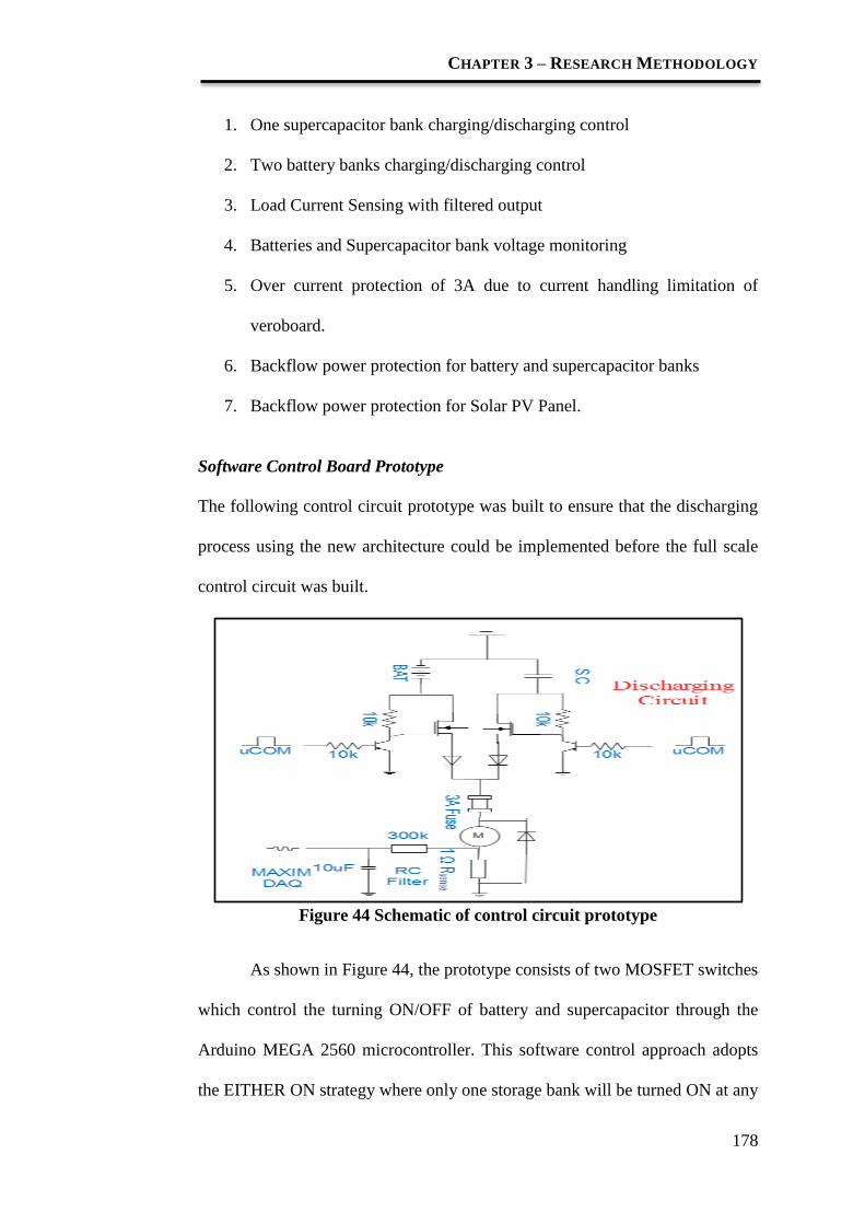
CHAPTER 3 – RESEARCH METHODOLOGY
178
1. One supercapacitor bank charging/discharging control
2. Two battery banks charging/discharging control
3. Load Current Sensing with filtered output
4. Batteries and Supercapacitor bank voltage monitoring
5. Over current protection of 3A due to current handling limitation of
veroboard.
6. Backflow power protection for battery and supercapacitor banks
7. Backflow power protection for Solar PV Panel.
Software Control Board Prototype
The following control circuit prototype was built to ensure that the discharging
process using the new architecture could be implemented before the full scale
control circuit was built.
Figure 44 Schematic of control circuit prototype
As shown in Figure 44, the prototype consists of two MOSFET switches
which control the turning ON/OFF of battery and supercapacitor through the
Arduino MEGA 2560 microcontroller. This software control approach adopts
the EITHER ON strategy where only one storage bank will be turned ON at any

CHAPTER 3 – RESEARCH METHODOLOGY
179
time. Hence, the voltage mismatch between supercapacitor and battery storage
will not pose an issue unlike the hardware approach which requires a DC/DC
converter to interface the battery with the supercapacitor.
P-channel MOSFET is chosen for switching as it is suitable for application
where load is directly connected to ground. However, the P channel MOSFET
requires a gate driver circuit which was formed of NPN BJT transistor and a
resistor tied to the source. Besides, a current sense resistor is also used as
voltage transducer for load current measuring. Lastly, protective measure was
also built into the system: the components such as diodes, freewheeling circuit
and fuse were used to prevent backflow power from load to storage supply. The
prototype built was based on the schematic shown in Figure 44. The prototype
which was built on the veroboard is shown in Figure 45 below:
Figure 45 Control Circuit Prototype
Full scale Software Control Board
The prototype control circuit only allows discharging control between the
supercapacitor banks and the battery bank. To ensure the integration of the solar
photovoltaic and HESS, complete software control circuit architecture which
3A Fuse
1Ω Resistor
P-channel
MOSFET
Current
Sense
Resistor
Diode

CHAPTER 3 – RESEARCH METHODOLOGY
180
enables the control of charging and discharging operation of the batteries and
supercapacitor bank. Besides, the software control board also allows alternate
battery to be charged by the solar charger while the other is supplying to the
Motor. By applying this multiple cell battery concept, downtime of the HESS
system during charging operation can be eliminated. Lastly, through the use of
SVR, the load current could be predicted multiple steps in advanced to allow
for intelligent turning ON of supercapacitor. This will improve the software
approach EMS time response. Figure 46 shows the schematic of the software
control board:
Figure 46 Schematic of software control board
As shown in Figure 46, the upper row of switches is designed for
charging control and the lower row of switches is for discharging control. In the
charging circuit, diodes are used to protect the Solar Panel from backflow
power from the battery and supercapacitor, while; in the discharging circuit,
diodes are used to protect the P-channel MOSFET from reversed high surging
voltage when the Motor is turned OFF. The presence of freewheeling diodes

CHAPTER 3 – RESEARCH METHODOLOGY
181
also ensures that the stored energy of inductive load is dissipating by the motor
itself rather than damaging the other components. A 3A fuse was used to
protect the software control board in case the Motor is drawing excessive
current. The battery and supercapacitor voltage sensors are excluded from the
circuit diagram for simplification purpose. The Software Control Board circuit
is shown in Figure 47:
Figure 47 Software Control Board
To measure the load current, a 1Ω current sensing resistor is used in
such that the voltage read out from the MAXIM USB 6009 DAQ will be
equivalent to the Motor current. As the DC Motor load is generally noisy, the
voltage across the current sensing resistor has to be filtered prior to the Analog-
Digital Converter (ADC). In such, low pass RC filter with cut off frequency of
fc ~ 1.5 Hz and 122 Hz are used to test their performance which is shown in the
Figure 48:
P-channel
MOSFET
P-channel
MOSFET
P-channel
MOSFET
P-channel
MOSFET
P-channel
MOSFET P-channel
MOSFET
Diode
Diode

CHAPTER 3 – RESEARCH METHODOLOGY
182
(a)
(b)
Figure 48 (a) RC filter with 122 Hz cut off, (b) RC filter with 1.5Hz cut off
(a) Fc =122 Hz load profile
readout
(b) Fc =1.5Hz load profile readout
Figure 49 RC filter performance comparisons
The same load profile was generated twice using the programmable
load. The first load profile and the second load profile is readout (retrieved) by
the Maxim USB 6009 DAQ with the RC filter with Fc=122Hz and 1.5Hz
respectively. As seen in Figure 49 (b), the load current profile using RC filter of
Fc = 1.5Hz is cleaner and has less harmonics noise. Another RC filter with Fc=
0.05 Hz was tested, it yield a clean DC value output but the response time is
much slower as the time constant of the RC filter has increased by 30 times.
Hence, for a good filtering performance and response time, the RC filter with
1.5 Hz was chosen to filter off the unwanted noises to ensure an approximately
DC output value.

CHAPTER 3 – RESEARCH METHODOLOGY
183
Programmable Load for prototype
In order to train and test the classification and load prediction accuracy
of the SVM, the load profile has to be replicated by using a programmable load.
To achieve this, 2 identical motors were clamped together along with a motor
driver to form a programmable load as follows:
Figure 50 Programmable load block diagram
The primary motor will be driven from the Software Control Board,
while the secondary generator will be driven by a motor driver that is
configured by the Arduino UNO. The motor driver was suplied by an external
power supply that is fixed to 13V and rated 1.6A to achieve a replicable load
whom torque generated will be consistent. The secondary motor will attempt to
rotate in the opposite direction of the primary motor according the PWM output
from the motor driver. However, the secondary motor PWM putput voltage
level was kept lower than the supply voltage from the primary motor. Hence,
the Secondary motor will act as a generator, and back e.m.f is fed into the
motor driver. However, by controlling the PWM output of the motor driver, the
back e.m.f level can be controlled and hence manipulating the load torque of
the primary motor. This will cause the current drawn by the primary motor to
be programmable. The actual programmable load was shown as follows:

CHAPTER 3 – RESEARCH METHODOLOGY
184
Figure 51 Programmable load
The programmable load was used to generate 5 different load profiles.
In order to synchronize the time when the programmable load and the MAXIM
DAQ sensing started, which is required for accurate classification, a signal will
be send from the arduino UNO to the arduino MEGA to contemporize the
operation between the two devices. The programmable load was coded in the
arduino environment to yield the load profile as in Figure 52:
Name Simulated load profile
Load 1
Load 2

CHAPTER 3 – RESEARCH METHODOLOGY
185
Load 3
Load 4
Load 5
Figure 52 Simulated load profiles
As shown in Figure 52, different load profiles that vary in time and
magnitude of the load current were simulated from the programmable load. The
load profiles could represent the different energy demand during weekday,
weekend, holiday and special events. For this project, only 5 load profiles were
simulated and trained with the SVMR-EMS for simplification and time
constraint reason. In real application, more profiles could be included into the
training to yield a more reliable load prediction. Load profile 1 represents
weekends as the power peak is highest among all other load profiles, load

CHAPTER 3 – RESEARCH METHODOLOGY
186
profile 2 represents days public holiday as the power peak is second highest
where the possibility of some people leave the house and go back hometown or
vacation; load profile 3 represents a long weekends or special months for
special festival such as Christmas, wedding and so; load profile 4 represents the
normal weekdays for working and school days as the power peak is the lowest;
load profile 5 represents the school holiday starts but no a public holidays as the
peaks also happen during daytime.
Since the programmable load generates the load current pattern through
PWM variation on the secondary motor, a certain issues has surfaced which
cause the replication of load profile to be rather difficult. Firstly, the power
supply for the motor driver has to be fixed to ensure the opposing torque
produced by the secondary motor remains consistent. Hence, an external power
supply with fixed voltage and maximum current limit is required for this task.
Secondly, the SLA battery voltage level drops as its discharging continuously
and this has cause the load current drawn by the primary motor to drop
accordingly. Hence, the load profile is not fully replicable for the training and
testing purpose. This adds to some difficulties in training and testing of the load
prediction. However, with the use of SVM which has excellent generalization
capability, the load prediction could still work well with the same load profile
which differs slightly due to the voltage drop as shown in the results section.
Determination of Time Respond Improvement Required
In the literature section, it was mentioned that a sequential programming that
adopts ‘monitor and respond’ strategy was implemented and the results shows a
70ms delay in the time response of the supercapacitor corresponding to the

CHAPTER 3 – RESEARCH METHODOLOGY
187
peak load current. However, in this project the software control board topology
and the constraint of charging and discharging for the battery and
supercapacitor bank was redesigned. Hence, it’s required that the time response
improvement needed to be known to estimate the K value required in the K
steps-ahead technique used in the SVR. By running the sequential programming
with the charging, discharging constraint, it is found that the time delay of the
supercapacitor corresponding to the peak load is around 200ms as shown in the
following:
Figure 53 Time Response of Supercapacitor with Sequential Programming
As shown in Figure 53, the Supercapacitor was turned ON 200ms after
the load current had met the peak load threshold value of 1.5 A (since 1 Ω
current sense resistor is used, the voltage is equivalent to the current value).
Hence, it is estimated that the K-value required is estimated to be 2-7 points
ahead (also means 200ms-700ms ahead) for the peak load prediction after
taking into account the classification and prediction processing time.

CHAPTER 3 – RESEARCH METHODOLOGY
188
Step 2: Load current prediction
The measure and respond strategy is deemed to have time delay and this shows
the need for SVMR_EMS to predict the peak load current in advanced to
improve the time response performance. As mentioned in the introduction
section, the load current in this project is simulated with programmable load
which has no external variable correlation with it except time and its own
previous values. Thus, it is proposed to use the K-step ahead autoregressive
model where the output variable is dependent only on its previous own values.
However, autoregressive model gives poor performance in nonlinear time series
modeling. Hence, the load forecast technique used in this project is the
autoregressive model of time series by using SVR to compensate the poor
performance of ARIMA in nonlinear domain as SVR has a good modeling of
nonlinear time series. Besides, due to the good generalization capability of the
SVR, the SVMR_EMS could still yield a good load prediction results albeit
there are inconsistency in the load profile generated.
The relationship between the SVR independent input variables and
dependent output variable by using the K-step ahead approach is shown in
literature section :
Y( t +K) = F(Y (t), Y (t −1). . . Y (t −m+1)) Equation 25
where K is the points in advanced of time to be predicted and m is the number
of previous points to be used for the next step prediction. Based on the time
response improvement requirement determined empirically, the K value was
chosen to be 7 and the m value to be 3. The implementation steps are explained
in Figure 54:

CHAPTER 3 – RESEARCH METHODOLOGY
189
Figure 54 The 7-steps ahead load prediction
As shown in Figure 54, the Maxim DAQ USB 6009 will scan for three
load current data points, and feed the data as the features of the input vector. By
mean of pattern recognition on the input features, it can be used to predict the
10th
point load current. This process will be repeated throughout the whole load
profile to give the SVMR_EMS the ability to predict the peak load current in
advanced. By implementing the 7-steps-ahead load prediction with 3 previous
variable values in the SVR, it has yielded a good supercapacitor time
performance as shown in the results Section 4.2.3.
Step 3: Support Vector Regression (SVR) Training & Testing
To implement the K-step ahead prediction for each load profiles, the SVR
model that describe the relationship between the previous 3 load current values
to the 7 points ahead load current value has to be trained and optimise to ensure
the model has good descriptive accuracy. There are 3 steps to the modeling
process: data preprocessing, model selection, and cross-validation and grid
search.

CHAPTER 3 – RESEARCH METHODOLOGY
190
1. Data Preprocessing
This step involves data acquisition, data adjustment for implementation of 7-
steps ahead forecast technique, and data format conversion to the required
format in LIBSVM. First, the Maxim USB 6009 DAQ was used to collect
the load current data from load profile 1 with a sampling rate of 10Hz by
using the Data_Collect.m written in MATLAB. Hence, there are in all 200
points of data for each load profiles. Second, the Data_Adjustment.m written
was used to prepare the input vector by making every 3 previous load current
value as the input feature variables. The output label linking each of the
input vectors will be the 7th
points in advanced load current value as shown
in the following:
Table 30 Data adjusted for 7 point ahead forecast
Finally, the dataset was converted into sparse format which is required
by the LIBSVM. By using the libsvmwrite (‘txt filename’, label vector,
instance vector) function provided, the dataset was converted into the
following format which could be readily read by the LIBSVM

CHAPTER 3 – RESEARCH METHODOLOGY
191
Figure 55 Sparse Format in LIBSVM
Scaling of the data is usually recommended prior to SVM training. This
is to prevent input attributes/features which have greater numeric value to
dominate the smaller ones. Besides, it could also improve the processing
performance, as big numerical value will cause the calculation of inner
product in the kernel to be difficult. Hence, it is recommended to scale the
data to the range (0-1) [101, 102]. However, in this project, only one single
variable is involved which will not cause any domination issue and the value
of the load current is only in the range of 1-3A which is considerably small.
Besides, the scaling also requires the real time downscaling of the input
current value which will add to processing requirement. The scaling process
was not applied in this project.
2. Model Selection
This step involves the selection of the suitable kernel model which is
available in the LIBSVM: linear, polynomial, radial basis function (RBF)
and sigmoid as mentioned in the literature review section. The RBF could
perform nonlinear mapping of the samples into a higher dimensional feature
space unlike the linear kernel. This gives the RBF a good nonlinear
modeling capability which suit the nonlinear time series forecast
requirement. Besides, the RBF has fewer tuning parameter than the
polynomial kernel which makes the selection of parameter process easier.

CHAPTER 3 – RESEARCH METHODOLOGY
192
Moreover, the sigmoid kernel faced some validity issues under certain
parameter condition [102]. Thus, the RBF kernel has been selected as the
primary choice. Yet, all kernels were tested for every single load profile
regression by selecting the kernel which yields the highest squared
correlation coefficient and lowest mean squared error. The squared
correlation coefficient (r2) shows the proportion of variance of output that
could be predicted by having the input. While, the mean squared error
(MSE) is a risk function that measure difference between the predicted
output and the true output [117].
3. Cross-validation and Grid-search
This step involves the search for best hyper/tuning parameter for the model
to predict the real time load current data accurately in every cases of load
profile. The hyperparameter serve to optimise the loss function on the
training dataset [250] . In the cross validation method, the dataset was split
into v portion: where (v-1) portions are for training and one portion is for
testing and validation. The accuracy of prediction obtained from the testing
set reflects the model’s ability to predict the unknown dataset, which
prevents the overfitting problem. For the load profile regression, the cross-
validation was done differently unlike the v-fold cross validation method
used in classification problem [251]. This is because only one load profile
dataset has to be included into the training set for autoregressive time series
prediction. Hence, the validation was done by another similar set of load
profile where there are slight differences due to the voltage drop. For the
parameters tuning, grid search was used along with the cross validation

CHAPTER 3 – RESEARCH METHODOLOGY
193
method. Pairs of the hyper-parameter/tuning values in exponentially growing
sequence were tested and the pairs which yield lowest mean squared error
was selected [96].
The five load profiles models was trained with the steps above and the
optimised parameter values for each load profiles were tabulated in result
Section 4.2.3.
Step 4: Load Profile Identification
After the 5 models for each load profile has been trained and optimise, the load
prediction could be performed excellently, provided that the correct load profile
model was chosen for the regression task. However, the load profile was chosen
manually and with the foreknowledge of the load profile generated by the
programmable load. This has a drawback of lacked of automation and the
choosing of load profiles could be difficult as there could be hundreds of load
profile in real application. In order to implement the SVMR_EMS with
complete automation, it has to be equipped with load profile identification
capability to ensure the load current prediction is based on the correct model.
Without the load profile identification, wrong models of trained load profile
could be used to predict the peak load current when real time data is polling
into the system. This will yield erroneous results as shown in the result Section
4.2.3.
The load profile identification by using SVM classification was done
through pattern recognition. Since every load profile exhibit different load
demand pattern, it is proposed that through classification of the pattern the load
profiles can be separated and identified. This can be implemented with the use

CHAPTER 3 – RESEARCH METHODOLOGY
194
of multiclass, multidimensional SVM. SVM was chosen for this classification
task as it has excellent generalization capability. Since this project deals with
real time peak load prediction, where the forecasting task will occur right after
the identification of SVR load profile model was made, its assumed that
beginning part of the load profiles holds a distinguish pattern which is
recognizable. For this, the load profiles simulated was designed to have
distinctive load pattern from each other at the beginning part for simplifying the
classification. Figures show the initial patterns suggested for the load profiles:
Figure 56 Initial pattern 1
Curr
ent
(A)
Time (s)

CHAPTER 3 – RESEARCH METHODOLOGY
195
Figure 57 Initial Pattern 2
In the initial pattern 1 (Figure 56), five of the load profiles start with
different load current rising gradient level as controlled by the programmable
load PWM; hence by recognizing the pattern of the first 100 data points, the
unknown load profile could be identified. However, since the load profile
replicability was influenced by the battery voltage level, it will yield erroneous
classification results when the battery voltage level dropped too much.
For this reason, the initial pattern 2 (Figure 57) was chosen as the
starting pattern of the five simulated load profiles. The load profiles have a
peak that differs from each other in terms of time. This pattern yields more
consistency for the classification as the battery voltage level drop will only
affect the peak load current magnitude but not the time of peak load occurrence.
Hence by recognizing the pattern of the first 100 points, the load profile could
be identified. In real application, the load profiles initial patterns are much more
complicated and require sophisticated data mining to generate a model that
could perform the load identification.
Curr
ent
(A)
Time (s)
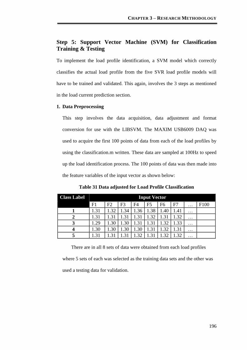
CHAPTER 3 – RESEARCH METHODOLOGY
196
Step 5: Support Vector Machine (SVM) for Classification
Training & Testing
To implement the load profile identification, a SVM model which correctly
classifies the actual load profile from the five SVR load profile models will
have to be trained and validated. This again, involves the 3 steps as mentioned
in the load current prediction section.
1. Data Preprocessing
This step involves the data acquisition, data adjustment and format
conversion for use with the LIBSVM. The MAXIM USB6009 DAQ was
used to acquire the first 100 points of data from each of the load profiles by
using the classification.m written. These data are sampled at 100Hz to speed
up the load identification process. The 100 points of data was then made into
the feature variables of the input vector as shown below:
Table 31 Data adjusted for Load Profile Classification
Class Label Input Vector
F1 F2 F3 F4 F5 F6 F7 … F100
1 1.31 1.32 1.34 1.36 1.38 1.40 1.41 …
2 1.31 1.31 1.31 1.31 1.32 1.31 1.32 …
3 1.29 1.30 1.30 1.31 1.31 1.32 1.33 …
4 1.30 1.30 1.30 1.30 1.31 1.32 1.31 …
5 1.31 1.31 1.31 1.32 1.31 1.32 1.32 …
There are in all 8 sets of data were obtained from each load profiles
where 5 sets of each was selected as the training data sets and the other was
used a testing data for validation.

CHAPTER 3 – RESEARCH METHODOLOGY
197
2. Model Selection
This step deals with the selection of suitable kernel which is used in the
model for classification of the load profile. The various kernels were tested
and the kernel with optimised parameter which yields the highest accuracy
with lowest number of support vector was chosen.
3. Cross Validation and Grid Search
For the SVM, the 8 fold cross validation was chosen, but instead of one,
three sets of data was used as the testing data while the other 5 sets was used
as training data. This allows the classification accuracy to better reflect the
model’s ability in classifying new data. Besides that, the best_parameter.m
in Matlab was used to perform the grid search which yields the optimise
value of C and g. The optimise SVM model was shown in the results section.

CHAPTER 3 – RESEARCH METHODOLOGY
198
3.2.3.2 Flow Chart of SVMR_EMS algorithm
With the establishment of the classification model and the load profile
regression models, the algorithm which includes the charging and discharging
constraint of the batteries and supercapacitor was written in MATLAB
environment, code name SVMR_EMS.m was shown as follows:
Figure 58 Algorithm of SVMR_EMS

CHAPTER 3 – RESEARCH METHODOLOGY
199
Algorithm Explanation
After the SVMR_EMS.m program in MATLAB was run, it will loop
continuously until a signal was send from the programmable load when the load
profile is started. Then Either the Battery A or Battery B will start to supply to
the motor load depending on the previous selection. The Maxim DAQ will also
pole the first 100 load current data points for the classification.
After the load profile is identified, The Maxim DAQ will continue to
pole 3 load current data points into the SVR model to predict the load current
which is 7 points ahead of time. If the predicted value is greater than the
threshold value set for the particular load profile, the supercapacitor terminal
voltage will be measured by the Arduino Mega 2560 to determine its SOC. If
the SOC level of supercapacitor is greater than 72% (equivalent to
approximately 10V), the supercapacitor will supply the load. If the SOC is
lower than 72%, the selected battery will continue to supply to the load while
the supercapacitor will be charged by the solar charger.
On the other hand, if the predicted value is lower than the threshold set
for the particular load profile, the Battery terminal voltage will be measured to
check its SOC. If the SOC level of battery 1 is < 80%, the battery 1 will be
flagged and charged up by the solar charger while battery 2 will supply to the
load. This will go on until the battery 2’s SOC is lower than 80%, then the
battery 2 will be flagged and start to be charged up by the solar charger. This
will simultaneously stop the charging of battery 1 and battery 1 will be selected
for the discharging operation. Meanwhile, the supercapacitor will be charged
whenever the battery is supplying to the load to ensure a more reliable supply

CHAPTER 3 – RESEARCH METHODOLOGY
200
from the supercapacitor when peak load is detected. This process will be
repeated until the program is shut off. The code is shown in Appendix A4.
3.2.3.3 Summary
The SVM is used for load identification and SVR is used for load prediction.
This load prediction software was implemented using LIBSVM in the
MATLAB environment.
Five important steps on implementing the software control box, data
acquisition device, microcontroller for the SB-HESS.
The energy control system allows the cost reduction in SB-HESS by
eliminating the power electronics to build bi-directional converter and also
avoid the direct coupling of a supercapacitor and battery energy source in
parallel.
SB-HESS with SVM_SRM allows load prediction which is used to avoid the
shortfall between the switching supercapacitor for peak power and battery
for the average power.

CHAPTER 3 – RESEARCH METHODOLOGY
201
3.3 Methodology Step 3
Identify the PV Standards, which governs the characterization of
supercapacitors used in PV systems
Reduction system cost by integrating the supercapacitor to the conventional
RES with the implemented SVM energy control system is shown in the
previous methodology steps. This part of the chapter emphasizes on the
manufacturing of fabrication supercapacitor. The aim of this step is to
manufacture supercapacitors, which have robust capacitance and voltage, and
which are economically feasible for solar applications. Supercapacitors are
manufactured based on the previous GA simulation in designing and optimally
sizing for the required specification of RES. Robustness in supercapacitor
fabrication is important. Since the energy stored in supercapacitors (shown in
Equation 2) is proportional to its capacitance and voltage squared, reducing the
maximum voltage of the unit will have a significant effect on its useable energy
density.
The fabricated supercapacitors conform to the British Standards IEC
62391-1, fixed electric double-layer capacitors for use in electronic equipment
– Part 1: Generic Specification and IEC 62391-2-1, Fixed electric double-layer
capacitor for use in electronic equipment – Part 2-1: Electric double – layer
capacitor for power application – Assessment level EZ.
Part 2.2 Preferred Values of Ratings of IEC 62391-1 is the standards,
which the fabricated supercapacitor is conformed to. It governs the preferred
rating and characteristic of supercapacitor which is used in solar system.
From IEC 62391-1, Part 2.2 [1],

CHAPTER 3 – RESEARCH METHODOLOGY
202
An integrated optimization approach is proposed in the supercapacitor
fabrication process. Genetic Algorithm is implemented within the Taguchi
method to optimise the process factor of supercapacitor fabrication. Orthogonal
array in Taguchi method is highlighted to reduce the number of experiments for
Design of Experiment (DOE) and GA is utilized to optimise the Signal-to-
Noise Ratio (SNR) in Taguchi method. SNR is an ideal metric for deciding the
best values, levels for the control process factors.
2.2.1 Rated capacitance (CR)
The rated capacitance shall be expressed in farads F) and as agreed
between the sending and receiving parties. Preferred values of rated
capacitance are the values from the E24 series of IEC 60063 and their
decimal multiples.
2.2.2 Tolerance on rated capacitance
The preferred values of tolerance on rated capacitance are: ±20 % and −20
%/+80 %.
2.2.3 Rated voltage (UR)
The rated voltage shall be as agreed between the sending and receiving
parties. The preferred values of the rated direct voltages are taken from
the R20 series of ISO 3 and their decimal multiples.
2.2.4 Rated temperature
The value of the rated temperature is 60 °C or 70 °C.
2.2.5 Internal resistance
The internal resistance shall be as agreed between the sending and
receiving parties. The internal resistance shall be measured with the d.c.
resistance method. However, if a coefficient can be obtained from both d.c.
and a.c. resistance methods, the a.c. resistance method may be used for
measurement.
Figure 59 British Standard IEC

CHAPTER 3 – RESEARCH METHODOLOGY
203
3.3.1 Process Fabrication Supercapacitor
This section reflects brief procedures of fabricating an electrochemical double
layer capacitor (EDLC). This supercapacitor fabrication process Table 32 (data
specification is retrieved from the bottle of the raw material) below shows the
material used in the process fabrication supercapacitor and the corresponding
supplier’s information.
Table 32 Raw Material used in Supercapacitor Fabrication
Material Supplier Details
Activated Carbon (AC)
for EDLC
RHE Resources
(Manufacturer’s
Origin: China)
Surface Area:
2000~2500 it was tested
in BET. bulk density:
0.4g/ml, Ash content:
<0.5%, moisture
content: <10%.
In a mixture of 10g
active material, 75% of
AC is used.
Carbon Black (CB) Cobalt - Vulcan
XC72R GP-3921 In a mixture of 10g
active material, 75% of
CB is used.
N-methyl-2pyrrolidone
(NMP)
Sigma-Aldrich 40ml of NMP (solvent)
is used for a mixture 10g
active material.
Polyvinylidene
Difluoride (PvDF)
Semyung Ever Energy
Co. LTD.
KF Polymer (Binder)
L#9130
Polymer content in 1g
of PvDF is 13%.
In a mixture of 10g
active material, 15% of
PvDF is used.
Filter Paper as
Separator Whatman Grade 1: 11m.
Dimension of the
separator used is 50cm x
3cm.

CHAPTER 3 – RESEARCH METHODOLOGY
204
Aluminium Foil as
current corrector
n/a Dimension of the current
collector coated is 40m.
Electrolyte 1M
Tetraethylammonium
tetrafluoroborate
(TEABF4) in PC
Semyung Ever Energy
Co. LTD.
n/a
Acetone
Sigma-Aldrich Assay 99.5, puriss p.a
*1. Bulk density is a property of powders, granules and other divided solids, especially used in reference
to mineral components, chemical substances, ingredients, foodstuff or any other masses of corpuscular or
particular matter. It is defined as the mass of many particles of the material divided by the total volume
they occupy. The total volume includes particles volume, inter-particle void volume and internal pore
volume.
2. p.a. pro analysis
The procedure of fabrication supercapacitor is presented as below:
1) The first step is mixing process where the activated carbon and carbon
black are assembled and weighted. The weighted activated carbon and
carbon black are dry-mixed for 10 minutes with the speed of 100 rpm
(revolution per minute). An overhead stirrer is used for this mixing process.
2) Next step is diffusion mixing by adding 40ml of NMP, which acts as a
solvent. It forms a homogeneous mixture. The mixing duration is 20
minutes and the speed used is 300rpm.
3) The binder PvDF is then added to the active material (the mixture). A
binder mixing process is required and it takes about 90 minutes at the speed
of 400rpm for this process.
4) The active material, which is in the form of slurry, is coated on the surface
of aluminium foil (current collector) using doctor blade (micrometer
adjustable film applicator) on a coater machine. The thickness of the slurry
coated on the current collector is 40µm. This desired thickness is set on the
micrometer adjustable film applicator, which has the adjustable thickness

CHAPTER 3 – RESEARCH METHODOLOGY
205
from 0.01mm - 5mm. This film applicator is pushed by the transverse
pusher to ensure constant speed coating.
5) The electrode (the coated aluminium foil with active material) is sent to the
vacuum oven for drying process. The temperature is set at 43°C for 5.5
hours.
6) The procedures of 1 to 5 are repeated for the backside of the aluminium
current collector.
7) The current collector is coated both front and back sides. This coated film
is called electrode. The electrode and the separator are cut.
Table 33 Length and Width of the Electrode and Separator
Length (cm) Width (cm)
Electrode 24 2.5
Separator 50 3
Figure 60 Supercapacitor Electrode

CHAPTER 3 – RESEARCH METHODOLOGY
206
Figure 61 Process of Lead Attachment using Ultrasonic Welder Machine
8) Next is the lead attachment process. A lead is attached onto each of the
electrode using ultrasonic welder machine as shown in Figure 61. This
process is repeated for the second strip of the electrode as two electrodes are
required to fabricate a full cell.
Figure 62 Seperator
(a) (b)
Figure 63 Cells and package
Electrode

CHAPTER 3 – RESEARCH METHODOLOGY
207
9) The separator as shown in Figure 63(a) is placed between the electrodes for
the coiling process is carried out. A clean tweezers is used to handle the
separators to prevent contamination. The end product for this process is
shown in the Figure 63.
10) The obtained EDLC coil is immersed in the electrolyte (1M TEABF4 in
PC). A rubber seal is placed on the leads and the cell is inserted into the
case. This is done to prevent the leakage of electrolyte.
11) Finally the cell is crimped and curled. An ID number is assigned to the full
cell for future tracking.
12) Test the performance of the cell using the potentionstat/galvaostat Autolab
PGSTAT302N in order to evaluate the capacitance and ESR of the cell. A
summary of the process shown in the table below:
Process Details Diagram
Weighing
materials
AC:75%,
CB:10%,PVDF:15%
Dry -
Mixing AC
and CB
Mechanical
mixing
10 minutes at 100rpm
Add 40ml NMP. Mix
for 20 minutes at
300rpm. Add PVDF
and mix for 90
minutes at 400rpm.
Coating the
aluminum
foil with the
active
material
Thickness of the
active material: 40μm.
Dry the
coating
43°C for 5.5 hours

CHAPTER 3 – RESEARCH METHODOLOGY
208
active
material
under
vacuum
oven.
Cut into
stripes with
the
dimension
of 24cm X
2.5cm
Two leads
are attached
onto the
electrode
foil.
Welding machine
A thin
separator
paper layers
interposed
between the
cathode and
anode foil
layers.
Winding machine
Figure 64 Steps of supercapacitor Fabrication
Supercapacitor Testing Procedure
Testing is particularly crucial for supercapacitor because it affects the
supercapacitor’s leakage current and life characteristics [53]. One of the
significant characteristics of supercapacitor is used to couple with battery is the
long cycle and shelf life. Devices with very low leakage current have a long life
as a low leakage current indicates the absence of low level Faradaic reactions

CHAPTER 3 – RESEARCH METHODOLOGY
209
between the electrode material and the electrolyte which over long periods of
time result in degradation of the devices. This means a reduction in capacitance
and an increase in resistance. This is very important in a hybrid energy storage
system as this SB-HESS is an optimised system. It affects the power delivery
time to cater for peak power. Supercapacitor is known as high power density
devices, it switches on instantaneously to cater for the peak power.
1. Brunauer-Emmett-Teller (BET) Analysis
The objective of carrying out this test is to evaluate the surface area of the
activated carbon used in the fabrication supercapacitor process. The surface
area analyser used is Micromeritics ASAP 2020 Accelerated Surface Area and
Porosimetry System V3.01 [252]. The commercial activated carbon is
purchased from Cobalt - Vulcan XC72R GP-3921. The BET model is one of
the commonly used equations for the calculation of the surface area of the
material [252]. The BET theory relates to the capacity of the monolayer formed
on a particular surface (the amount of the adsorbed molecules in the monolayer)
[252]. The equation is not covered in this thesis. The crucial value for this
research is the BET surface area 2010.6896 m2/g. The BET analysis is still the
existing standard method of examining the surface area of materials as other
methods might not provide better advantages over BET analysis. For this test,
the setting is shown as follows:
Sample Mass: 0.0926 g
Cold Free Space: 90.5136 cm3
Low Pressure Dose: None
Analysis Adsorptive: N2
Analysis Bath Temp.: -195.842 °C
Thermal Correction: No

CHAPTER 3 – RESEARCH METHODOLOGY
210
Warm Free Space: 28.8193 cm3 Measured
Equilibration Interval: 10 s
Automatic Degas: Yes
2. Cyclic Voltammetry
Generally, capacitance and Equivalent Series Resistance (ESR) are the main
output response in this process fabrication supercapacitor. The cyclic
voltammetry technique is one of the methods used in this project to obtain
output responses of the supercapacitor. In this technique, potential applied to
the electrode immersed in the organic or aqueous electrolyte is varied with the
time and the relevant current-potential curves recorded. The linear sweep
voltammetric technique is used in all testing the capacitance of the
supercapacitor fabricated. The electrode potential is set from an initial value Ei
to an ending value Ef at a constant scan rate, s. The equation is shown below:
Equation 42
When the potential value Ef is met, the direction of the scan is inverted
[253]; while still keeping the same scan rate, s, and the potential is returned to
the beginning value (cyclic voltammetry).
With the relation to the equation of
and Equation 43, we can
derive the two following Equations 43 and 44.
Equation 43
Equation 44

CHAPTER 3 – RESEARCH METHODOLOGY
211
If C is constant with potential, then a rectangular current response
against the potential would be generated, where the shape would be
symmetrical around the zero-current line [253], given that the scan rate remains
the same for both anodic and cathodic scans [254]. However, in most cases, C
would not be constant with reference to the potential in the scan and the sweep
rate, due to the kinetic or diffusion limitations of the current [254]. The electric
current, I can be defined as the electric charge, q in coulombs transferred in t
seconds, i.e.
Equation 45
Replacing Equation 44 and Equation 45 into Equation 46 and cancelling the dt
term, the following term can be obtained:
Equation 46
It follows that to obtain an average value of capacitance from the cyclic
voltammogram which includes a positive and negative scan, the following
equation can be utilized, i.e.
where q+ and q
- are the anodic and cathodic voltammetric
charges on the anodic and cathodic scans respectively.
Equation 47
The cyclic voltammetry was performed in this project using scan rates
between 2mV/s, 5mV/s, 10mV/s and 20mV/s.

CHAPTER 3 – RESEARCH METHODOLOGY
212
(a)
(b)
Figure 65 Autolab PGSTAT302N
3. Galvanostatic Charge-Discharge Test
According to the dissertation [254], the galvanostatic charge-discharge
technique often applies in the application of a constant current source across the
electrochemical cell and the recording of the potential response. When a
constant current, i, is applied in an interfacial charging process, accumulation of
charges ∆q takes place across the interface to an extent that it is dependent on
the potential of the electrode related to the potential difference built up across
such an interface (∆V) [255]. This implies the equation below:

CHAPTER 3 – RESEARCH METHODOLOGY
213
Equation 48
And ∫ Equation 49
Therefore, ∫
where ∆t is the time interval taken to reach the particular
potential
Equation 50
As in the case of cyclic voltammetry an ideal rectangular
(voltammogram) [253] , Equation 50 implies for capacitance which is constant
with potential. However, from the test profile shown in section later, this is not
the case, so ∆V diverges from a linear dependence on time at a constant current.

CHAPTER 3 – RESEARCH METHODOLOGY
214
3.3.2 Optimising Process factor using The Taguchi-GA method
Previous applications [256, 257, 258, 259] indicate that the Taguchi
method emphasizes the solution of single-response problems with the aid of
knowledge gained from past experience. Thus, it is not capable of handling
multi response problems without requiring some modifications in the
application.
The Taguchi method provides practitioners and designers with a
systematic approach for conducting experiments to obtain near optimal settings
of design factors for performance and cost [260, 261, 262] . The design
(controllable) factors and noise (uncontrollable) factors, which influence the
quality of the product, are considered together instead of individually [259,
263].
The objective of implementing the Taguchi method is to obtain the best
combination of factors and levels in order to achieve the most robust product.
This means, the selected levels of the various design factors from the Taguchi
method allows the performance of the product/process to be less sensitive to the
noise factors.
However, in today’s manufacturing environment, many processes or
products involve solving multi response problem to improve their product
quality. One crucial fact is that the Taguchi method is incapable of performing
well for multi-response optimization problem [260, 261]. In order to overcome
this limitation, we have formulated a way to include a GA within the Taguchi
method.
A common method of solving the multi response problems is to assign
each response with a weight, as mentioned in [260, 261, 264]. A normal

CHAPTER 3 – RESEARCH METHODOLOGY
215
question which arises is how to determine and define the weight for each
response in a real case. The goal of this proposed strategy is to ensure that the
performance characteristics (or the quality) have minimal variation while
having its mean close to the desired target value.
The idea underlying this integrated strategy is to convert the problem of
optimising a complicated multi process response into one that optimises a
single weight of the SNR. This means, the weighted signal-to-noise ratio,
WSNR is used in the overall evaluation of experimental data in the multi
response optimization problem. In this case, the GA strategy utilizes the
normalised SNR (Z) from the Taguchi method to form its fitness function. The
optimal level for each individual process factor is the level with the highest
WSNR.
Design of experiments (DOE) is a method that can be used to identify
the critical areas that cause yield loss in a process. With proper application of
DOE, design engineers or researchers are able to pinpoint the source of the
yield problem and fix them to produce solid and robust designs with much
higher yield [265]. In DOE, the three terms that need to be clearly defined are
Factors, Levels and Replication. Factors or parameters are important variables
that would affect the outcomes or output responses. However, all factors may
not have equal importance as some factors may have a more prominent effect
over other factors. ‘Levels’ in the simplest terms are possible values for each
factor identified thru gathered data (for this case the levels are ‘low’ and
‘high’). For example, if two levels are assigned to each factor, one of the lower
levels is a lower level and the other is a higher level. The values of these levels
are assigned in reference to literature, consultation with experts or one can

CHAPTER 3 – RESEARCH METHODOLOGY
216
identify level values thru experimentation before the Taguchi method is carried
out [256, 266]. A two-level factor assumes linear behavior while three-level
factor best fits non-linear behavior but requires a larger number of trials while
running experiments. Replication is necessary to address the concern on
repeatability and also the spread of the variation in the experimental outcome.
This is done in order to obtain adequately accurate statistical information of the
process under study. This is done by producing several samples for each trial or
by repeating the same trial several times.
The Taguchi method is famous for implementing robust (parameter and
tolerance) design. Robust design is a result of determining the optimal factor
combination/setting to reduce the response variation and brings the mean close
to the target value consequently [267]. To implement the robust design,
Taguchi employs an orthogonal array (OA) in order to reduce the number of
experiments as compared to the full factorial DOE version. SNRs are used to
evaluate the outcome of the experimental trials. It is common to include an
ANOVA alongside SNR to study the percentage contribution made by each
factor. Even though the Taguchi method has been successfully applied to
processes in design and manufacturing, it has been criticized for its lack of
efficiency because the method works well for single-objective optimization
problems but not for multi-objective problems [12, 268]. Some modification on
the existing method has to be made [261, 269, 270, 271] to make it work for
some cases of multi objective problems.
Similarly, the Taguchi method for multi-objective problems, as
discussed by Phadke as mentioned in [270], is purely based on judgmental and
subjective process knowledge [272]. When dealing with a multi-objective

CHAPTER 3 – RESEARCH METHODOLOGY
217
problem, one can use several techniques. The simplest way is by adopting the
OEC (overall evaluation criteria) approach. This is done by assigning certain
weighting to each of the output response criteria so as to normalize the two (or
more) different response units. The weightings are arbitrarily chosen based on
experience in order to make a response either dominate or have the same weight
when compared to the other responses [265, 273, 274]. Such judgments are not
very accurate [272]. A way of overcoming this problem is by using the GA
approach. In section below, the GA method will be further discussed
specifically on how it was used with the Taguchi method to make solving the
multi-objective problem possible. The GA will search for the optimal weights
that maximize the SNR for each output response to improve its immunity to
noise and thus make the product more robust. The hypothesis here is that the
GA approach will result in a better SNR as compared to the OEC (initial
method) as stated in Table 80 (Chapter 4) method because the GA searches the
entire solution space for the optimal point whereas the weights determined by
experience does not. To proof this hypothesis, the percentage improvement of
the SNR (if any) will be determined and then the process parameters will be
implemented to confirm the increase in robustness of the product.
In this case, the integrated approach is divided into several repeatable
steps that could also be applied in other process/product multi-objective
optimization problem accordingly. There are four steps outlined (Step 1-4
mentioned below) for the initial experimental factors and levels design,
including the computation of SNRs from the experimental data. Next, the
integration of GA approach for determining the optimal weights based on the
normalised SNRs (Z) in the range between zero and one are conducted (Step 5-

CHAPTER 3 – RESEARCH METHODOLOGY
218
6). The WSNR is then computed by multiplying the weight with Z relates to
each response. The final two steps (Step 7-8) will be the data analysis focusing
on the main effect of each factor towards the WSNR values, which is essential
for predicting the desired optimal setting. It continues with the confirmation
experiments. Consequently, further statistical data analysis includes the
measure of variability between OEC and the proposed strategy is conducted
using standard deviation and ANOVA, in order to determine the percentage
improvement acquired (if any) and subsequently identify the dominant factors
that influencing the capacitive performance of the device.
The implemented Taguchi-GA method is applied in supercapacitor
fabrication and the steps fall within the initial experimental design stage, are
listed below.
3.3.2.1 Steps Implementing the Taguchi-GA Method
Step 1: Assigning factors and levels for each of the main processes
Table 34 provides the lists of control factors for mixing, calendaring, drying
and electrolyte treatment process. All of the three factors (A, B and C) are
assigned with two levels of factor each for the experiment. The rationale of
choosing the Level 1 and Level 2 is based on the senior’s experience in this
fabrication process. For this study, the value of Level 1 and Level 2 were
selected based on the parameters shown in [275]. For future work, if time and
cost are allowed, more levels for the process factors could improve the output
response.

CHAPTER 3 – RESEARCH METHODOLOGY
219
Table 34 Process factors and their levels for the supercapacitors fabricated
Process Factors Level
1
Level
2
Output Response
1
Mixing
A Mixing Speed (rpm)
B Mixing Time (min)
C Amount of AC (%)
200
15
85
350
30
90
1. Capacitance (F)
2. ESR (Ω)
2
Calendaring
A Calendaring time (min)
B Thickness (mm)
C Machine temperature (oC)
15
0.65
23
30
0.85
30
3
Drying
A Heating time min)
B Heating temperature (oC)
C Vacuum
20
50
Yes
45
80
No
4
Electrolyte
Treatment
A Electrolyte name
B Electrolyte molarity (M)
C Electrolyte amount (ml)
KCl
2
0.5
Na2S
O4
3
0.8
Step 2: Determining the minimum number of experiments required and the
selection of Taguchi orthogonal array.
Here, the Taguchi multi-objective optimization begins with the selection of
orthogonal array (OA) with specific number of levels (L) for factors A, B and
C. The minimum number of experiments in the array is obtained by using the
equation below [12]:
( )
where F = number of factors, in our case, F = 3
Equation 51
Thus, L4 orthogonal array (OA) is selected due to four numbers of trials
required and outlined as in Table 35. The selection of OA depends on the
number of factors to be studied as shown in the Equation 51, the number of

CHAPTER 3 – RESEARCH METHODOLOGY
220
interaction to be studied, time and cost constraints.
Table 35 4 x L4 Orthogonal arrays for the process factors
Process Experiment, i A B C
1
Mixing
1
2
3
4
1
1
2
2
1
2
1
2
1
2
2
1
2
Calendaring
1
2
3
4
1
1
2
2
1
2
1
2
1
2
2
1
3
Drying
1
2
3
4
1
1
2
2
1
2
1
2
1
2
2
1
4
Electrolyte
Treatment
1
2
3
4
1
1
2
2
1
2
1
2
1
2
2
1
Step 3: Conducting all experiments outlined with three replications (samples)
each according to the Level which is assigned to the Factors shown in Table 34.
Value of level 1, level 2 and factors for each of the process are defined in Step
1.
Step 4: Computing SNR for every output responses.
The SNR values for the respective responses (SNiC and SNiE) are calculated
from the raw data from the experiment accordingly. The equations are shown
below:
SNR for the capacitance response (larger-the-better)
SNiC = -10 ( )∑
Equation 52

CHAPTER 3 – RESEARCH METHODOLOGY
221
SNR for the ESR response (smaller-the-better)
SNiE = -10 ( )∑
where yi is the experimental data at the ith sample and n is the
number of samples.
Equation 53
The Integrated Taguchi method with GA
The main aim of integrating the GA into the Taguchi technique is to search for
definite and optimal weights for each response or performance characteristic
and quality) in a multi-response system. As previously stated [12, 259, 263,
264], the Taguchi method has been mostly utilized in optimising single-
response problems. One of the noted methods in tackling multi response
systems is the problem of optimising weights for signal to noise ratio as
mentioned in the literature [256]. In real multi-response cases as described in
[12, 276], the weights are based on experience. For instance, in the OEC
approach the relative weighting method is used to tackle problems with more
than one objective [263]. The method of combining multi criteria of evaluation
is truly based on the expertise and the experience gained in many experiments.
However, in most real cases this does not result in a robust process or product.
This might be due to a level of uncertainties in the decision-making stage
especially when picking levels for the parameters. Furthermore, it is difficult
for human experts to estimate the effect of the criteria used to evaluate a
process as not all criteria have equal importance. As such, the key of obtaining
a robust and practical process using this weighting method may be to eliminate
the engineering judgment in deciding the weights (or the importance) of the
criteria.

CHAPTER 3 – RESEARCH METHODOLOGY
222
The GA is a powerful heuristic global search and optimization
technique. It is an optimization technique which is built based on mimicking the
evolutionary principles and chromosomal processing in natural selection and
natural genetics [6]. It is a widely accepted approach to stochastic optimization,
especially in dealing with a global optimization problems that consists of multi-
modal search spaces. In a wider usage of the term, GA is any population-based
model that uses selection and recombination operators to generate new sample
points in a specific search space [277]. In his book [6], Goldberg demonstrated
the possible domains where GA’s can be applied. Moreover, many GA models
have been introduced by researchers and are found to be effective from the
experiment perspective [277]. In addition, many of them are application
oriented and have adopted GA’s as optimi ation tools [261, 11, 278]. The
searching and selection of optimal weights for the process of fabrication of
supercapacitors using the Taguchi method often involves problems related to
constrained optimization which is similar to what is needed in manufacturing
process optimi ation. Hence, it is appropriate that GA’s are integrated with the
Taguchi method to optimise the fabrication of coin-type supercapacitors. The
capacitance and equivalent series resistance (ESR) of the device are adopted as
the quantitative performance characteristic (quality) for evaluation in the
current study.
GA’s basically evolved from an idea of survival of the fittest and
reproduction of new offspring to form a new population to create a novel and
innovative search strategy [261, 279, 278]. It implies that the genetic pool in
GA of a given population potentially contains the solution, or a better solution,
to a given adaptive problem [277, 279]. This makes the GA different as

CHAPTER 3 – RESEARCH METHODOLOGY
223
compared to other traditional point-to-point descending and ascending search
techniques [280]. The GA initiates from a random set of solutions, known as
the initial ‘population’. Each individual solution in the population is known as a
‘chromosome’ or string). At each generation, the GA works with genetic
operators namely crossover and mutation, on the selected individuals which act
as parents to recombine part of the strings genes) and produce offspring child)
to create a new and hopefully fitter generation [6, 281]
During each generation, these chromosomes evolve to have better
fitness. This is done by executing an operation known as selection. Eventually,
the chromosomes in the population will converge from generation to
generation. The aim is to select the best fit chromosome [266, 6, 281]. By
fulfilling the aim mentioned, GA utilizes the fitness function (or objective
function) which will be used to create a new and conceivably better population
of strings. The fitness function takes a chromosome and assigns a relative
fitness value to the chromosome [6]. The fitness function evidently ranks the
chromosome in some way by producing fitness values [10].
Step 5: Normalizing the SNRs so that all are in the range between 0-1.
Normalised yij as Zij [0, 1] by the corresponding formula to set the right effect
of adopting different units, where i is the number of experiment (i.e. number of
sample) and j is output response of the process. In this case, output response is
capacitance and equivalent series resistance. Notation used in the equations
below is C and E. The selection for Equation 54 is based on the fact that the
output response of capacitance is expected to be as higher as possible for
supercapacitor fabrication because this study is to maximize the capacitance by

CHAPTER 3 – RESEARCH METHODOLOGY
224
optimising the setting configuration of the experiment [275]. However, the
quality characteristic selected for the SNR is smaller the better, hence, Equation
55 is selected. This is because the output response ESR is expected to be as
smaller as possible, therefore it is able to enhance pulse current handling by
parallel connection with an electro-chemical battery [275].
Normalised SNR for the capacitance response (the-larger-the-
better) [13];
= ( ) ( )
Equation 54
Normalised SNR for the ESR response (the-smaller-the-better)
[13];
= ( ) ( )
where Yavg is the average out of the n number of samples
produced, Ymin and Ymax are the least and highest data value out
of the n number of samples produced respectively.
Equation 55
Step 6: Searching for the exact/optimal weighting value w associated with each
Z that would give the maximum WSNR by using GA approach.
The WSNR value is determined by using the weights (wc and wE) obtained from
GA.
WSNRi = wCZiC + wEZiE
where i is the number of runs/experiments
Equation 56

CHAPTER 3 – RESEARCH METHODOLOGY
225
In the section below, GA is used to maximize WSNRi with the optimal wC and
wE.
Initialization
The algorithm is carried out randomly to create the solution space which is used
for searching the optimal weights so as to maximize Z. In this coin
supercapacitor fabrication process, we have two output responses; hence there
are only two weights which are considered as the gene. The initial population
composes of 30 chromosomes. The 30 chromosomes in the initial population
are generated subject to the feasibility condition, i.e. the sum of weights should
always equal to one.
The Fitness Function
The total WSNR is used as the fitness function in GA strategy to calculate the
fitness value. A fitness value in an objective function evaluates the performance
level of an individual chromosome; therefore in this case, GA strategy utilizes Z
from Taguchi method to form this fitness function. The particular fittest
chromosome will be ranked against all other individual chromosomes. The
fitness function is given as:
F(x) = ∑ ∑ ( )
Equation 57
The Equation 57 above is written such that f(x) is the total WSNR to be
maximised, wij is the weight to each response, Zij is normalised SNR values, n is
numbers of observation (experiments/runs) and k is the number of response.

CHAPTER 3 – RESEARCH METHODOLOGY
226
Selection
Selection is also known as reproduction in the family of computational model
inspired by evolution [281]. It allows individual (string/chromosome) to be
copied for possible inclusion in the next generation. The chance that a string
will be copied is based on the string’s fitness value which is calculated from the
fitness function. For each generation, Selection chooses strings that are placed
into the mating pool, which is used as the fundamental to create the next
generation. Parent chromosomes are selected with a probability related to their
fitness value. Therefore, highly fit strings possess the higher probability of
being selected for mating [281]. In this supercapacitor fabrication process, the
roulette wheel method is applied to the chromosome selection.
Crossover
Once the mating pool is created using Selection operator, the next operator is
the crossover. The term ‘Crossover’ used in GA is analogous to reproduction
and biological crossover. ‘Crossover’ is used to create a pair of offspring
chromosome from the parent chromosome [281]. Crossover takes place by
depending on the parameter known as the crossover probability, Pc [12]. If the
crossover does not take place, two selected chromosomes are simply copied to
the new population. The concept of this operator is the new chromosome may
be better than both of the parent chromosomes as the offspring takes the
goodness from each of the parents.

CHAPTER 3 – RESEARCH METHODOLOGY
227
Mutation
One-gene mutation operation with a preset mutation probability Pm which
indicates the frequency at which mutation occurs is applied to generate a new
chromosome [12]. Pm should be preset at a very low value. In this case,
mutation is performed during the crossover. Mutation occurs when a new
gene’s value is added to the new population pool. This is to avoid the
population stagnating at any local optima [277].
Check for feasibility (constraint of the algorithm)
This is a step to obtain reliable and feasible weights for the fitness function. In
this case, this step is crucial to ensure that the sum of the weights is always
equal to one. This step is to encounters 3 possible cases mentioned below.
Case 1 - the sum of the gene values of offspring is less than one.
If the sum of the gene values of offspring is 0.9; there is a shortage
quantity of 0.1 (since 1 -0.9 = 0.1). The shortage quantity will be
equally divided, and added equally to the gene values.
Case 2 - The sum of the gene values of offspring is more than one.
If the sum of the gene values of offspring is 1.2, there is an excess
quantity of 0.2 (since 1.2 – 1.0 = 0.2). The excess quantity will be
equally divided, and added equally to the gene values.
Case 3 - The sum of the gene values of offspring equal to one, the gene
values will remain the same.

CHAPTER 3 – RESEARCH METHODOLOGY
228
Stopping Condition
The most usual and popular method – setting the maximum number of
generation is used for the stopping condition. This can guarantee the
convergence of a GA. In this case, the stopping condition is the total number of
generations fixed at 10,000 [6].
Step 7: Study the main effects on WSNR for each factor and level by plotting the
Factor Effects on WSNR graphs. This will lead to our predicted optimal
conditions.
WSNR is similar to the overall evaluation of experiment (OEC) data for a
multi-response process but the weightings used are the main difference. The
level for each factors with the highest WSNR is the optimal level (optimal
setting for the particular process) of process factors. The computation of the
main effect on WSNR is carried out by considering the average effect of each
level with respect to each factor. Details and result are discussed in Section
4.3.2. For example, for Process 1 (Mixing), A1 means the average value of
WSNR1 and WSNR2 for Level 1 of the process factors where Level 1 is
remained unchanged in that experiment, however the value of other process
factor is changed. This is to evaluate the interactions of the process factor. This
concept is applied to other average WSNR (A1, A2, B1, B2, C1, C2 ). These
values also known as corresponding factor effects. The larger the WSNR
implies the better quality. This is a step leads to select the optimal condition of
the process.

CHAPTER 3 – RESEARCH METHODOLOGY
229
A1 = (WSNR1+ WSNR2) / 2 Equation 58
A2 = (WSNR3+ WSNR4) / 2 Equation 59
B1 = (WSNR1+ WSNR3) / 2 Equation 60
B2 = (WSNR2+ WSNR4) / 2 Equation 61
C1 = (WSNR1+ WSNR4) / 2 Equation 62
C2 = (WSNR2+ WSNR3) / 2 Equation 63
Step 8: Running the confirmation experiment and compare the results
(Standard Deviation and SNR) with the earlier trials and initial condition.
Figure below tabulates the summary of the steps mentioned above.
Figure 66 Figure: Flow Chart of the Integrated Taguchi-GA method
Define the process factors, levels and output responses
Step 1: Experimental design using Taguchi method
1. Orthogonal array experiment. 2. Computation of SNR. 3. Transformation of SNR to Z.
Step 2: GA approach
1. Determine optimal weights wc, wE) corresponding to each process. 2. Compute the WSNR for each process.
Step 3: Continuation of Taguchi method
1. Identify main effect factors on WSNR. 2. Predict the optimal condition.
Step 4: Statistical data analysis
1. Conduct confirmation experiments. 2. Compute Standard deviations. 3. ANOVA – identify significant factors.
Optimal process factors

CHAPTER 3 – RESEARCH METHODOLOGY
230
3.3.3 Summary
The integrated Taguchi and GA method is used to optimise the process factors
of supercapacitor fabrication process.
The Taguchi-GA integrated strategy provides a robust design in the sense of
reproducibility and reliability. This could not be achieved by the OEC
approach alone as this approach is dependent on engineering judgment (that
has higher variation), a mean value that is far from the desired target value if
those judgments were inaccurately made.
This methodology step is important because noise factor in the manufactured
values will cause failures in matching peak demand as the hybrid energy
storage system is optimised using the GA. Hence a slight drop in capacitance
and ESR will cause the reliability of the system.
The methodology step is important to reduce spread in tolerance of
supercapacitor value (capacitance and ESR) which will affect the optimization
in sizing RES and power reliability of the system.

CHAPTER 3 – RESEARCH METHODOLOGY
231
3.4 Methodology Steps 4
Construct lab scale prototype design and fabrication
The optimised supercapacitor-battery hybrid energy storage system (SB-HESS)
is tested on a lab scale trolley. The configuration of the system was explained in
the Chapter 1-Introduction. The optimal sized of lab-scale SB-HESS is design
and integrated with the unsupervised learning machine - Support Vector
Machine of energy management system (SVM_EMS). Details on the energy
management system are elaborated in Section 3.2.3. The integrated architecture
was designed as shown in the following:
Figure 67 Integrated System on Trolley
3.4.1 Final Testing
The prototype system is tested with the performance metric shown below.
There are three main testing for this prototype.
The performance metric used in system is categorized into 3 groups: One
for the performance definition of the SVM and SVR.
Monitor
Supercapacitor
Battery
Programmable
Load –
Arduino Uno
DC/DC
Converter
Software
Control
Board
Maxim
USB 6009
DAQ
Motor
Driver
Clamped
Motor

CHAPTER 3 – RESEARCH METHODOLOGY
232
Performance comparison between the standalone battery storage and hybrid
energy storage in terms of cost and battery lifetime.
The reliability and efficiency of HESS using SVMR_EMS and a HESS
using hardware-based (DC/DC converter) approach.
1. Mean Absolute Percentage Error (MAPE)
MAPE error is the accuracy measure for technique used in modeling time
series. It is expressed as the average of the total difference in percentage as
shown in the following:
∑
where LR is the actual value of load current and LP is the value
of predicted load current
Equation 64
Comparison Performance Metric
1 Energy management system
Support Vector Machine
Classification Accuracy
Number of Support Vector
Training Time
Support Vector Regression Mean Average Percentage Error
MAPE)
2 Standalone battery storage system
and hybrid storage system State of Charge SOC)
System Cost
3 Software Approach and
Hardware Approach for energy
management system EMS)
Supercapacitor Time Response
Power Efficiency
System Cost

CHAPTER 3 – RESEARCH METHODOLOGY
233
Besides that, n is the number of points to be compared. Hence, by this
formula, the accuracy of the predicted load current can be measured.
2. State of Charge (SOC) stress test
The SOC of the standalone battery storage system and hybrid
supercapacitor- battery storage system using hardware and software approaches
were recorded for performance comparison. To implement this, a stress test of 1
minute pulse current cycle which is catered for high discharge rate and high
depth of discharge (DOD) of the battery. The high discharge rate will reduce
the stratification effect but will lead to high sulphation of the battery which give
a greater negative impact on the battery. Besides, the high DOD will also lead
to sulphation of the battery [282]. The stress test load profile was simulated
using the programmable load as shown in Figure 68.
Figure 68 Stress Test Load Profile
The standalone battery system will supply for the whole load cycle,
while; in the hybrid system, the battery will supply only when load demand is
below the threshold value and supercapacitor will supersede the battery role in
supplying for load demand above the threshold value. The battery will first be
charged with a fixed charging characteristic of 14V, 1A to ensure the

CHAPTER 3 – RESEARCH METHODOLOGY
234
consistency of fully charged battery voltage level as the battery final open
circuit voltage varies with the charging rate. Besides, the battery is allowed to
stabilize before attaining the SOC value. The battery will then undergo the
stress test for 20 cycles. This process was repeated 4 times for the standalone
battery system and the hybrid system.
By implementing the combination of Open Circuit Voltage method and
Current Integration Method, a more accurate SOC monitoring system can be
achieved. The SOC is measured using Open Voltage Method during unloaded
operation and Current Integration method during loaded operation. In this
project, the Maxim DS2438 Smart Battery Monitoring Evaluation Kit is used.
This Chip can measure the battery voltage and current, the accumulated current
flowing in or out of the battery with the integrated current accumulator, and the
battery temperature with the on board direct to digital temperature sensor. The
data acquired will be stored on the chip’s onboard memory and will be
transmitted through one wire interface which provides versatile operation with
any microprocessor/microcontroller [283]. Since the EV kit comes with a
window GUI and DS91230 serial to USB converter, it allows direct
configuration and monitoring of the Battery SOC on the GUI as shown below:
(The evaluation kit used is MAXIM DS2438EVKIT+. The evaluation kit is
interfaced to a PC through a DS91230 USB adapter and RJ-11 cable
connection).

CHAPTER 3 – RESEARCH METHODOLOGY
235
Figure 69 Circuit connection for MAXIM DS2438EVKIT+
This smart battery monitoring system is able to measure the
temperature, voltage, current of the lead acid battery. Apart from that, it is also
able to set the elapsed-time in order to be able to synchronize with the real time
and able to log all data in a text file. Figure 70 shows the meters screen which
displays the real time measurements of the battery voltage, temperature, current
and remaining capacity of the lead acid battery.
Figure 70 Meters screen of DS2438EVKIT+

CHAPTER 3 – RESEARCH METHODOLOGY
236
A certain configuration is needed to measure the lead acid battery
during charging and discharging phase as shown in Figure 71.
(a) Charging (b) discharging
Figure 71 Connections to simulate the charging and discharging phase of
the battery
However, the maximum voltage that can be measured by this evaluation
kit is 10V and the lead acid battery is rated at 12V. Therefore, a voltage divider
circuit is made to reduce the lead acid battery voltage by half. Two 500 Ω
resistor is used for the voltage divider.
3. Supercapacitor Time Response
The Supercapacitor Response Time is the most important performance
measure in this project. As mentioned earlier, the replaceability of the hardware
DC/DC converter with the software approach lies in the successfulness of
supercapacitor to response corresponding to the peak load demand. In the
hardware approach, the switching action of the DC/DC converter is in a matter
of milliseconds. Hence it has good time response but with the tradeoff of
having more expensive power electronics which added to the cost of the overall
system. In the software approach, the time required for the control includes the
load current data acquisition time, storage banks voltage monitoring time,

CHAPTER 3 – RESEARCH METHODOLOGY
237
processing time and control switches responding time which are reflected in the
supercapacitor response towards the peak load demand. The previous sequential
based programming shows a delay of 70ms which will not meet the
requirement in rapid burst load application. Hence, the adoption of SVR to
predict the load current will give a buffer time for the SVMR-EMS to
compensate the control time required; allowing the supercapacitor to be
switched ON before the peak load demand occurs. Since the battery will be
turned OFF when supercapacitor is ON, the load current will be supplied only
from the supercapacitor. Hence, to measure the response, the voltage supplied
by supercapacitor and the load current will be probed on the oscilloscope to
measure the difference between the supercapacitor turn ON time and the Peak
Load demand occurrence time. In Figure 72, the supercapacitor response time is
shown.
Figure 72 Supercapacitor Respond Time
4. Power Efficiency
Besides comparing the supercapacitor time response of the SVMR-EMS, the
power efficiency between the hardware DC/DC converter approach and the

CHAPTER 3 – RESEARCH METHODOLOGY
238
software approach are also compared. The power efficiency is defined as the
ratio of the power delivered to the load over the input power as follows [284]:
η = 100% · Pout / Pin
where Pout is the output power and Pin is the input power.
Equation 65
As mentioned in the literature review section, the hardware approach’s
switch mode DC/DC converter has efficiency range of 75-98%. while; the
software approach has voltage drop across the diode, current sensing resistor
and the power losses associated with stray resistance in the circuit, hence the
power supplied that actually reaches the load has to be measured in both cases
to form a comparison. On the other hand, the software approach’s Software
Control Board has MOSFET switches and backflow protection diode and a
1ohm current sensing resistor. The MOSFET has resistive element and
conduction losses is proportional to its on resistance RDS (ON), the current
sensing resistor causes a voltage divide drop, and the diode has a 0.6V forward
voltage drop. Besides, both approaches exhibit power losses which associates
with the non-idealities such as stray resistances which has also contributed to
the overall efficiency drop. As the load current is either supplied by the
supercapacitor or battery, the load terminal voltage alone will determine the
efficiency of the system.
5. System Cost
The system cost is one of the performance metrics for comparison
between hardware and software appraoch energy management system (EMS).

CHAPTER 3 – RESEARCH METHODOLOGY
239
As this project seeks the feasibility of software approach to replace the costly
power electronics in the hardware approach, the cost of both system will have
to be compared to justify the use of software approach in the EMS. The unit to
measure the system cost of two different aprroaches used for the prototype
system is in Malaysia Ringgit (RM).
Last but not least, cost of supercapaitor-battery hybrid energy storage
system and battery individual system are compared. The system cost reduction
resulting from minimizing the number of replacement battery for 20-years are
shown in Chapter 4.
3.4.2 Summary
This methodology step is a final integration and testing step. This step
shows the feasibility and reliability of the implemented SB-HESS.
In this section, five performance measures are used to measure the
accuracy of load prediction system, the system cost, the state-of-charge
(SOC) battery for of SB-HESS and battery-alone system, time response of
the supercapacitor to react peak power and power efficiency of the systems.

CHAPTER 4 – RESULT AND DISCUSSION
240
CHAPTER 4
RESULT AND DISCUSSION
This chapter tabulates results that address the problem statements and principal
aim stated in Chapter 1. The purpose of this chapter is to discuss the result
obtained from the implementation steps shown in Chapter 3. The section is
organized as follows:
Section 1: presents the optimal operation parameters for the
supercapacitor-battery hybrid energy storage system (SB-HESS) and
how this SB-HESS benefits the battery lifespan.
Section 2: The design and simulation for RES is presented using
HOMER. HOMER is used to that our GA is working properly by
comparing results between HOMER and the GA for battery-only
system. The optimal cost of SB-HESS is presented and compared with
the conventional renewable energy system (RES) using a genetic
algorithm (GA). GA is used to design the prototype before it is
implemented. There is trade-off between the system cost and the Loss of
Power Supply Probability (LPSP). Simulation results show that if the
LPSP is 100%, the system cost is higher than the system with 98%
LPSP. GA acts as a searching algorithm is capable to search the
optimised number of components used in the system at the lowest cost
whish subject to constraints and the desired LPSP. GA optimises battery
lifespan and evidently, the system cost.

CHAPTER 4 – RESULT AND DISCUSSION
241
Section 3: discusses the energy control system for SB-HESS using the
Support Vector Machine (SVM) and how this implemented system
benefit the system cost (prolongs battery life and reduces number of
power electronics) and system reliability (predict time to turn on
supercapacitor before power peak delivery is needed). The system cost
is said to be optimised where the system cost for the SB-HESS
prototype is compared with the conventional system which energy flow
is controlled by DC/DC converter. The results shows that the system
cost is lower than the conventional system. This is because the
implemented energy management system using SVM and relay switches
successfully control the energy flow between the energy storage system
and load while further optimises (reduces) the number of costly power
electronics used. This section also shows the comparison of state-of-
charge (SOC) of battery in both battery individual system and SB-
HESS.
Section 4: Shows the result on the performance of the supercapacitor
fabricated in the supercapacitor pilot plant in terms of capacitance and
equivalent series resistance (ESR). The implemented optimization
technique combining Genetic Algorithm within Taguchi Signal-to-
Noise ratio is proven in designing a robust process.

CHAPTER 4 – RESULT AND DISCUSSION
242
4.1 Determination of Optimal Parameter for Energy
Management System
This section presents the result of optimal parameter for designing the energy
management system (EMS) for this project. These parameters also identify the
benefits of coupling supercapacitor with battery in a energy storage system.
One of the crucial parameters in this energy management system is voltage
level of battery. This value is always kept at a nominal value according to the
depth-of-discharge (DOD) that it favors. This is done to ensure the
implemented hybrid energy storage system (HESS) aids in prolonging the
battery lifespan by limiting the voltage of batteries and hence, the system is
setting an optimal set point for the SOC batteries. In a battery-alone system, the
batteries are stored and drained to release energy to match the load demand at a
short period. The conventional battery-alone system can be costly as compared
with the SB-HESS. The main focus in SB-HESS is the delivery power peak by
supercapacitors while the battery releases energy in a desired time and in a
controlled manner. This implemented system is practical because the
supercapacitor delivers power 99% accurately as this energy management
system also predicts load beforehand as mentioned in Section 3.2.3. The price
of battery is much higher than supercapacitor terms of kW/$ as supercapacitor
has higher power density.
Therefore, an optimal voltage value is important for the implemented
EMS to evaluate the depth to which a battery can safely be depleted. To further
protect the battery from over-discharging, this implemented EMS prevents
operation beyond the specified end-of-discharge voltage, which is obtained
from the manufacturer data sheet. The end-of-discharge for a 1.2Ah battery is

CHAPTER 4 – RESULT AND DISCUSSION
243
1.75V/cell. This approach has been proven in Section 4.4 that it reduces the rate
of damage mechanism of battery as mentioned in Section 3.1.
A high load current lowers the battery voltage, and the end-of-discharge
voltage threshold should be set lower accordingly to cater that particular power
peak in a conventional battery-alone system. However, in SB-HESS, a desired
battery voltage which has been calculated is always above the final discharge
value given in manufacturer data sheet. The battery in SB-HESS discharges at a
nominal value of current for a prolonged time, it evidently causes less impact
on the rate of damage mechanism of the battery. The strategy applied also
ensures the battery always discharge at a constant optimal C-rate (according to
technical manual of GP battery) to supply load and the battery final discharge
voltage is not bounded by zero volts at any time. C-rates means charge and
discharge rate of the battery. In this project, discharging phase is focused.
In SB-HESS, a higher and desired end-of-discharge voltage of batteries
is maintained. This tells us that the voltage of the so-called healthier battery
gradually recovers and rises towards the nominal voltage repeatedly. However,
in long run, battery in a conventional battery alone system becomes aging more
rapid and this aging battery with elevated self-discharge cannot recover the
voltage. Battery used in our lab-scale prototype system is shown below:
Table 36 Data Specification of Battery
Manufacturer GP Lead
Capacity 1.2Ah
Nominal Voltage 12
Final discharge Voltage 1.75
The result shows in Table 36 is calculated using the semi-empirical
Equation 4 shown in Section 3.1, it shows that battery current (Ibatt), voltage of

CHAPTER 4 – RESULT AND DISCUSSION
244
the cell (Vcell) and voltage of the battery (Vbatt) is always below 1.6Amps, 2.07V
and 12.41V respectively for the implemented EMS. This provides a clear view
for designing the optimised prototype system where how much battery capacity
can be used for delivering to the load and how many supercapacitors are
required for delivering the power peak. Moreover, it also provides the important
parameter to implement energy control management system for the load
predictive software to predicts when the supercapacitor is switched on and cater
for the peak power. Table 37 below shows the calculated and optimal
parameters for supercapacitor-battery hybrid energy storage system.
Table 37 Theoretical values for parameter Ibatt, Vcell, Vbat
Parameters Battery individual energy
storage system
Supercapacitor-Battery
hybrid energy storage
system
Ibatt (A) 2.5 1.6
Vcell (V) 1.99 2.07
Vbatt (V) 11.99 12.41
From the result above, it can be represented in the diagram shown
below. Different level of current for battery-only system and SB-HESS are used
to implement the prototype.

CHAPTER 4 – RESULT AND DISCUSSION
245
Battery-individual system Implemented HESS
= supplied by the Batteries.
= supplied by batteries,
= supplied by supercapacitors.
‘C’ for a 1.2 Ah battery, for example, is 1
– 1.2 amps. Full discharge is reached after
about 30 minutes when the battery voltage
drops to 1.5V/cell. At this point, only 50%
of rated capacity has been discharged
(1 C amps x 0.5 hrs = 0.5C Amp. Hrs).
Continuing the discharge to zero volts will
bring to the total amount of discharged
ampere-hours (capacity) to approximately
75% because the rapidly declining voltage
quickly reduces current flow to a trickle.
‘C’ for a 1.2 AH battery, for example, is
0.3 amps. Full discharge continuing
discharge the battery (to zero volts) on
the battery is never happened as the
supercapacitor acts as a high power
density energy storage device to cater the
power bursts.
Battery voltage remains at about 2V/cell.
At this point, only 20% of rated capacity
has been discharged
(0.25 C amps x 0.5 Hrs. = 0.125C Amp.
Hrs.).
Figure 73 Energy flow for battery-only and SB-HESS
The diagrams in Figure 73 above shows two different cases. From the
diagram, the C-rate is different for two cases shown above because the required
battery capacity for both cases is different. This also implies that the battery
DOD for both cases is different as more battery capacity is used up in Case 1 to
deliver the peak power in short period. By considering a same load profile,
batteries in battery-individual system are delivering the power peak and the
battery is drained to release energy over a short period of time. As mentioned

CHAPTER 4 – RESULT AND DISCUSSION
246
previously, a high load current lowers the battery voltage, and the end-of-
discharge voltage threshold should be set lower accordingly to cater the power
peak. The battery discharges to a lower load current as the supercapacitor
delivers power peak for the same high load current. It does not damage
supercapacitor, as it is known as an ideal energy storage that undergoes
frequent charge and discharge cycles at high current and short duration. This is
due to the nature of supercapacitor that stores energy by means of a static
charge as opposed to an electrochemical reaction.
This shortens battery life when the batteries are stressed and drained to
supply the entire power bust of the load demand profile over a short period of
time (for battery single energy storage system). For a higher discharge rate (1C-
rate) (Case 1), it causes a hard and irreversible of sulphation. When the battery
is not operated at a high discharge rate and the battery remains at a low state-of-
charge (SOC) for a long period of time, the sulphate crystals grow in size and
large sulphate crystals are created. Since these large crystals do not dissolve
easily when the battery is charged, this eventually leads to hard or irreversible
sulphation [32]. Evidently, it causes a loss of battery capacity because the
sulphated part of the active material is no longer active and the large sulphate
crystals grow into part of the insulated active material from the terminal
electrode. Furthermore, the sulphate crystals have a larger volume than PbO2
(and Pb), which causes a higher mechanical stress on the electrodes. This
sulphate crystal causes inhomogeneous current distribution. The longer time at
low SOC accelerates the hard and irreversible sulphation of battery.
Result in this section identifies the optimal parameter to design the EMS
for this project. A comparison for the implemented system is presented in

CHAPTER 4 – RESULT AND DISCUSSION
247
Section 4.4. Table 102 shows the remaining state-of-charge (SOC) of a battery
individual system and the supercapacitor-battery hybrid energy storage system
after running on a same load profile for every 20 cycles. The remaining
capacity of battery (indication of SOC) drops more in a battery single energy
storage system compare with the SB-HES.
4.1.1 Summary
The high load current for an instantaneous power delivery elevates the
discharge rate and current of the battery. This damages battery more rapidly.
Supercapacitor in SB-HESS delivers instantaneous power. It aids in
prolonging battery lifespan by catering for the peak power.
A higher end-of-discharge voltage for battery is guaranteed in SB-HESS.
The calculated value is 12.07V and it is used in designing the EMS for this
project.

CHAPTER 4 – RESULT AND DISCUSSION
248
4.2 Cost Structure of Renewable Energy System
Current cost structure for renewable energy system (RES) is simulated using
HOMER and Genetic Algorithm (GA). The optimization results are presented
in Section 4.2.1 and 4.2.2 respectively. Both methods are able to show the
optimised cost of the PV-Wind-Battery and PV-Battery system. Simulation
process models a particular system configuration; the optimization process
determines the best possible system configuration. Due to the limitation of
HOMER of adding supercapacitor as energy storage device, GA fitness
functions were constructed to optimise the supercapacitor-battery hybrid energy
storage system (SB-HESS). System cost of the supercapacitor-battery hybrid
energy storage system in RES is lower than the battery alone RES. RES is also
optimised subject to the desired loss of power supply probability (LPSP) and
capacity shortage. The higher the capacity shortage, the lower the system cost.
The result is shown in the section below.
Furthermore, the SB-HESS embraces the green technology by reducing
the total number of batteries used throughout the lifespan of the system.
Implemented energy control system using unsupervised learning machine,
SVM for supercapacitor-battery hybrid energy storage system (SB-HESS) is
also proven to further reduce the overall system cost and increase the power
reliability of the system in Section 4.2.3.

CHAPTER 4 – RESULT AND DISCUSSION
249
4.2.1 Optimal Sizing of RES using HOMER
The optimum sizes of the system that meet the load profiles at the proposed
site, given conditions of renewable energy resources and based on components
data sheet were simulated using HOMER. HOMER provides the results in
terms of optimization and sensitivity analysis. These results a component size
(optimization and a sensitivity analysis) for three cases (Case 1: capacity
shortage of 0%, Case 2: capacity shortage of 1% and Case 3: capacity shortage
of 2%) are presented in section below. These three cases for this simulation is
based on the fact that in the Tenth Malaysia Plan (2011-2015), Malaysia
government emphasizes greatly on improving energy efficiency, sustainability
achieved through energy efficiency [285]. Therefore, a zero downtime of power
system (Case 1) is suggested in this study. This also means the 0% LPSP, one
optimal set of configuration of a hybrid energy storage system can technically
guaranteed the required reliability of power supply. As mentioned in [161], for
a stand-alone system simulation, capacity shortage is often set up to a
maximum of 2% as shown in [239] study for an allowable unmet load hour.
Hence, for case 2 and 3 in this project are suggested because 1% and 2%
shortage of power supply is considered low impact on the downtime (power
reliability of system) as mentioned in [239]. This also implies that the capacity
shortage percentage recommended in [239], blackouts is still possible but for a
very small percentage of the time [225].

CHAPTER 4 – RESULT AND DISCUSSION
250
Case 1: PV-wind-battery with capacity shortage of 0%
This system is designed and constraint for a 0% capacity shortage. A capacity
shortage is practically zero means there is no shortfall at any time between the
required and the actual operating capacity.
1. Optimization Result
In HOMER, the best possible (optimal) system configuration is the one that
satisfies the user-specified constraints at the lowest total net present cost.
Finding the optimal system configuration involves deciding on the
combination of components that the system should contain, the size or
quantity of each component. In the optimization process, HOMER simulates
many different system configurations, discards the infeasible ones (those that
do not satisfy the user-specified constraints), ranks the feasible ones
according to total net present cost, and presents the feasible one with the
lowest total net present cost as the optimal system configuration.
Figure 74 shows the design of the battery alone system with PV panel
and wind generator, which was simulated in HOMER. Primary Load 1
represents the load demand with 50% of discrepancy of the simulated load,
Converter represents the DC/DC converter, PV represents the photovoltaic
panels of the system, Generic 1kW represents the wind turbines and H200
represents the batteries used. A feasible system is defined as a hybrid system
configuration that is capable of meeting the load.

CHAPTER 4 – RESULT AND DISCUSSION
251
Figure 74 Block diagram of PV-wind-battery energy system
Figure 75 Optimization result for PV-wind-battery system (0% of capacity
shortage)
The optimization result for the RES shown in Figure 74 is tabulated in
Figure 75. From the optimization result shown above, the global solar
radiation is 5.4kWh/m2/day. This annual mean value is taken at the site
shown in Section 3.2 – Semenyih, which is 4.12kW. Generally, optimization
result shows feasible and optimised system. In Figure 75, it shows two
RESs, one is PV-Wind-Battery system and one is PV-Battery system. The
terms show in the figure above can be explained as follows:
Table 38 Indication for Optimization result in Figure 75
Column Shown in Figure 75 Indication
First column Presence of PV panels
Second column Presence of wind generators
Third Column Presence of battery storage
Forth Column Presence of converter

CHAPTER 4 – RESULT AND DISCUSSION
252
Fifth Column Size of the PV array in kW
Sixth Column Number of the wind generator
Seventh Column Number of the batteries utilized
Eighth Column Size of the converter in kW
Ninth Column Dispatch Strategy
Tenth Column Initial cost of the System
Eleventh Column Operating Cost per year
Twelfth Column Total net present cost
Fourteenth Column Cost of Electricity ($/kW)
Fifteenth Column Renewable Energy Fraction
Sixteenth Column Battery lifespan in terms of years.
The project lifetime is 20 years, which follows the lifespan of the PV
panel. Based on the optimization result, the PV-wind-battery power system
comprised of 2kW PV array, 1 wind generator, total of 20 batteries used in
addition to 2kW converter is found to be the most optimal and feasible
system with a total minimum net of present cost (NPC) of $44,114 in the
entire cycle life of the system. The optimization result is simulated according
to the data input on the specification of the components, which is presented
in Section 3.2.1. Renewable energy fraction (Ren. Frac.) shown in the
fifteenth column in Figure above is renewable fraction of the system which
is based on the amount of the renewable energy that supplies goes towards
serving the primary load. The renewable fraction is 1.00, which means there
is no diesel generator used in the system. This means there is no gas
emission from the system, such as carbon dioxide, carbon monoxide,
unburned hydrocarbon, sulphur dioxide and nitrogen oxide.

CHAPTER 4 – RESULT AND DISCUSSION
253
The dispatch strategy used is cycle-charging strategy. HOMER offers
two dispatch strategies, which are called load-following and cycle-charging.
Under the load-following strategy, a generator produces only enough power
to serve the load, and does not charge the battery bank. Under the cycle-
charging strategy, whenever a generator operates, it runs at its maximum
rated capacity (or as close as possible without incurring excess electricity)
and charges the battery bank with the excess. Barley and Winn [166] found
that over a wide range of conditions, the better of these two simple strategies
is virtually as cost-effective as the ideal predictive strategy that is how the
idea is inspired by adding a supervisory machine learning system to control
the energy flow in our renewable energy system). Because HOMER treats
the dispatch strategy as a decision variable, the modeler can easily simulate
both strategies to determine which is optimal in a given situation [14].
This means that under cycle-charging strategy used in this study, the
system runs at full power and charge the battery with any excess. With the
cycle charging strategy you can apply a setpoint state-of-charge, so that the
energy sources or generators keep charging the battery and the battery is not
allowed to discharge until it has reached the setpoint. This strategy is
appropriate to use for this project because the implemented load predictive
energy management system control the flow of energy from battery state-of-
charge.
COE is the cost of the electricity. For the simulated PV-wind-battery
system, the COE is $1.115/kWh. This is lower than systems with diesel
generator, for example in [228], the COE is much higher ($25.41). This is
because the use of diesel fuel is expensive and the price of fuel is increasing

CHAPTER 4 – RESULT AND DISCUSSION
254
over the years. In this site location, the solar irradiance is optimum for solar
energy system.
Figure 76 Cash Flow Summary of PV-Wind-Battery System
Figure 76 depicts the cash flow summary of the system. From the plot,
total cost of the battery (H150 in the plot) which combines initial capital
cost, replacement cost, operational and maintenance (O&M) cost gives the
highest impact in the overall cost of system.

CHAPTER 4 – RESULT AND DISCUSSION
255
Figure 77 Electrical power for PV-wind-battery system (capacity shortage
0%)
Figure 77 depicts the excess electricity, unmet load, capacity shortage
and renewable fraction for the most economically feasible system. It can be
seen from Figure 77 that with the above system configuration, unmet load is
0 kWh and an excess energy of about 10.6% is generated. It should be
mentioned here that this excess energy produced goes to waste due to lack of
demand. This figure also summarizes that the monthly average PV generated
power is much higher as compared to wind energy for this selected site as
the velocity wind at this selected site is low. However, the solar irradiance is
high to provide 96% of the renewable energy to the system.
2. Sensitivity Analysis
Sensitivity analysis helps assess the effects of uncertainty or changes in the
variables over which the designer has no control, such as the average wind

CHAPTER 4 – RESULT AND DISCUSSION
256
speed or the future fuel price. In this case, fuel price is not considered. One
of the primary uses of sensitivity analysis is in dealing with uncertainty and
evaluates trade-off in capacity shortage, capital cost, maintenance cost,
operational cost and replacement cost.
Figure 78 Sensitivity results for PV-wind-battery system (capacity shortage
of 0%)
According to the simulation result, it tells us that the system without
wind turbine is more favourable as the wind velocity is low in the selected
site. It is not cost-effective in adding wind turbine to the system at this site.
The COE is lower than the PV-wind-battery system, $1.009/kWh. The net
present cost is $39939 as shown in the Figure 78. The figure below shows
zero unmet electrical load and zero capacity shortage for this system.

CHAPTER 4 – RESULT AND DISCUSSION
257
Figure 79 Electrical power for PV-battery system (capacity shortage of
0%)
Figure 80 Cash flow summary for PV-battery system (capacity shortage of
0%)

CHAPTER 4 – RESULT AND DISCUSSION
258
From the figure above, overall cost of battery is still the highest among
the other components even wind generator is not included in this system.
This means that operating reserve (in this case is battery only) is large
enough and always available for the system. Hence, there is no unmet load
throughout the years.
Case 2: PV-wind-battery with capacity shortage of 1%
This system is designed and constraint for a 1% capacity shortage. The capacity
shortage fraction (C.S.F) is the fraction of the total load plus operating reserve
that system fails to supply. If a system is ever unable to supply the required
amount of load plus operating reserve, HOMER records the shortfall as
capacity shortage. Operating reserve is the surplus electrical generation capacity
(above that required to meet the current electric load) that is operating and able
to respond instantly to a sudden increase in the electric load or a sudden
decrease in the renewable power output. For this case study, the C.S.F was
taken equal to 1%.
1. Optimization
Figure 81 Optimization result for PV-wind-battery system (1% of capacity
shortage)
Generally, the indication on the columns is same as those mentioned in
Table 38. From the simulation result for this case, the NPC is $42882. The

CHAPTER 4 – RESULT AND DISCUSSION
259
total NPC is slightly lower as there is a shortfall that occurs between the
required amount of operating capacity load plus required (operating reserve)
and the actual operating capacity the system can provide. The number of
batteries used is less compared to Case 1. Operating reserve is the amount of
operating reserve that a power system provides is equal to the operating
capacity minus the electrical load. Operating reserve is surplus electrical
generating capacity that is operating and responds instantly to a sudden
increase in the electric load or a sudden decrease in the renewable power
output. This means operating reserve is the fraction of the primary load that
hour, plus a fraction of the annual peak primary load, plus a fraction of the
PV power output that hour, plus a fraction of the wind power output that
hour. In this case, operating reserve is obviously lower than the previous
case as the capacity shortage is 1%. A high operating reserve increases the
unnecessary system cost with oversized system.
The battery lifespan is shorter in case 2 as compared to case 1. The
expected battery lifetime is 10 years in case 1, whereas in case 2 (with
capacity shortage of 1%), the expected battery lifetime is 6 years only. This
causes higher battery replacement cost.

CHAPTER 4 – RESULT AND DISCUSSION
260
Figure 82 Electrical power for PV-wind-battery system (capacity shortage
of 1%)
The unmet electric load is 1% as initially the capacity shortage was set
to 1%. The difference between case 1 and case 2 is the COE and operating
cost. The COE is lower in case 2. However, the operating cost in case 2 is
high as mentioned earlier, the high number of replacement battery causes
high replacement cost and O&M cost. This can be optimised using a load
predictive energy control management system and adding high power
density and less maintenance energy storage devices, such as supercapacitor.

CHAPTER 4 – RESULT AND DISCUSSION
261
Figure 83 Cash flow summary of PV-wind-battery system with capacity
shortage of 1%
The initial cost of the batteries is less compare to the system in case 1.
This is because less number of batteries are considered in this case as the
operating reserve is lower with the capacity of shortage is set to 1%.
However, the battery lifespan is evidently short compare to the first case
where the number of battery used is 20 for the initial instalment of the
system. The initial set of the batteries are drained as low operating reserve is
designed and set. This also leads to high replacement cost and O&M cost of
the battery throughout the 20 years.

CHAPTER 4 – RESULT AND DISCUSSION
262
2. Sensitivity analysis
Figure 84 Sensitivity results for PV-wind-battery system (capacity shortage
of 1%)
A system without wind turbine in the selected site is more feasible in
terms of NPC. The NPC of RES with capacity shortage 1% is lower than the
system in Case 1. The NPC is $39376 for this RES model. The unmet load
shown in Figure 82 is lower than the PV-wind-battery system (capacity
shortage of 1%) in Figure 79.
Figure 85 Electrical power for PV-battery system (capacity shortage of
1%)

CHAPTER 4 – RESULT AND DISCUSSION
263
Figure 86 Cash flow summary for PV-battery system (capacity shortage of
1%)
Figure 86 shows the cash flow summary for the PV-battery system
(capacity shortage of 1%). By observing Figure 80 and Figure 86, about 37%
of the total system cost is caused by the initial, operational and maintenance
cost of the batteries.
Case 3: PV-wind-battery with capacity shortage of 2%
Final design, simulation and optimization is done by changing the constraint in
HOMER, which represents capacity shortage of 2%. It is clearly shown that
PV-battery system has lower system cost (net present cost) compare to the
previous cases. On the other hand, PV-wind-battery has the same total system
cost as shown in case 2.

CHAPTER 4 – RESULT AND DISCUSSION
264
1. Optimization
Figure 87 Optimization result for PV-wind-battery system (2% of capacity
shortage)
Figure 87 shows the net present cost for PV-wind-battery with (capacity
shortage of 2%) is the same as the in case 2 (PV-wind-battery with the
capacity shortage of 1%) which is $42882. From the simulation results
shown in Figure 88, it tells us that the insignificant unmet load (also known
as capacity shortage) for this proposed power system has no impact on the
system cost. This means that to allow a smaller, less expensive power
system, the proposed system with capacity shortage of 2% is not feasible and
cost-effective to increase the operating reserve(number of battery) to satisfy
the unmet load.
Figure 88 Electrical power for PV-wind-battery system (capacity shortage
of 2%)

CHAPTER 4 – RESULT AND DISCUSSION
265
Based on the Figure 89 below, the initial cost of the battery is lower as
compared to the initial cost for battery in case 1. However, the replacement
cost of the battery is much higher in case 2 and case 3. This is due to the
higher usable capacity of battery in case 2 and case 3. Hence, the expected
lifetime of battery is shorter. This also means that the number of replacement
batteries is higher in this case.
2. Sensitivity Analysis
Based on the three figures below, the NPC for this system is the lowest
compare to the systems in case 1 and case 2. The NPC of this system is
$38557. This always depends on the system specification which is designed
by the user. It is a trade-off between the price that the user can afford and the
power shortage and delivery.
Figure 89 Cash flow summary for PV-wind-battery system (capacity
shortage of 2%)
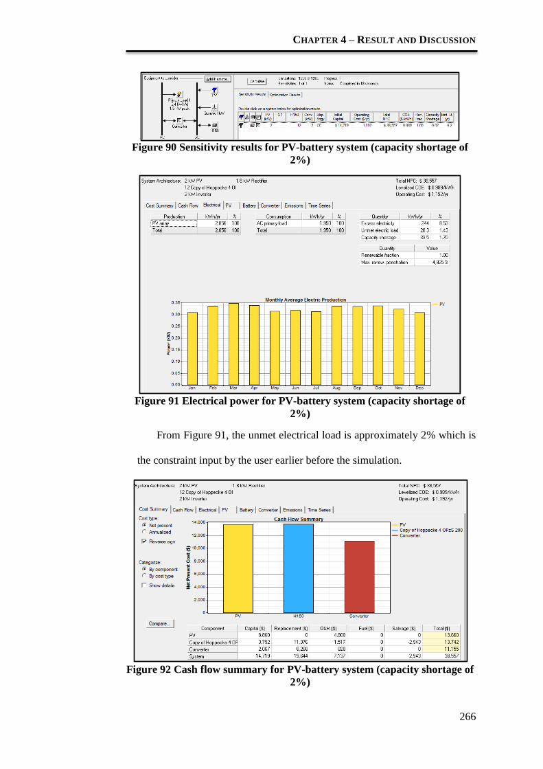
CHAPTER 4 – RESULT AND DISCUSSION
266
Figure 90 Sensitivity results for PV-battery system (capacity shortage of
2%)
Figure 91 Electrical power for PV-battery system (capacity shortage of
2%)
From Figure 91, the unmet electrical load is approximately 2% which is
the constraint input by the user earlier before the simulation.
Figure 92 Cash flow summary for PV-battery system (capacity shortage of
2%)

CHAPTER 4 – RESULT AND DISCUSSION
267
This system is feasible even without wind generator as mentioned
earlier; the wind power at this site does not contribute high generated power.
Hence, systems is said to be more cost-effective and optimised according to the
sensitivity results shown in. with only 1.70% of capacity shortage throughout a
year.
4.2.1.1 Summary
HOMER is a good tool to design, simulate, optimise and sensitively analyse
different parameters for power systems. To limit input complexity, and to
permit fast enough computation to make optimization and sensitivity
analysis practical, HOMER’s simulation logic is less detailed than that of
several other time-series simulation models for micropower systems, such as
Hybrid2, PV-DesignPro, and PV*SOL. On the other hand, HOMER is more
detailed than statistical models such as RETScreen, which do not perform
time-series simulations. Of all these models, HOMER is the most flexible in
terms of the diversity of systems it can simulate.
From the three cases simulated above, batteries always cause the highest
impact in the overall cost for a long-term renewable energy system for this
project (20 years is considered).
The batteries cost mainly are from replacement cost, operational and
maintenance cost. This can be optimised by adding a high power density and
less maintenance energy storage device, such as supercapacitor. It is
mentioned (in the next section). This could improve battery lifespan.
Table 39 shows the net present cost for three cases mentioned in this section.

CHAPTER 4 – RESULT AND DISCUSSION
268
Table 39 Net Present Cost of different RES (found by HOMER)
No. Renewable
Energy
System
Net Present
Cost ($)
Battery
Initial Cost
($)
Battery
Replacement
Cost ($)
Estimated
Battery
Lifespan
(years)
1 PV-wind-
battery with
0% capacity
shortage
44114 6320 6320 10
2 PV-battery
with 0%
capacity
shortage
39939 6320 6320 10
3 PV-wind-
battery with
1% capacity
shortage
42882 3792 11376 6.3
4 PV-battery
with 1%
capacity
shortage
39376 5056 10112 8.1
5 PV-wind-
battery with
2% capacity
shortage
42882 3792 11376 6.3
6 PV-battery
with 2%
capacity
shortage
38557 3792 11376 6.2

CHAPTER 4 – RESULT AND DISCUSSION
269
4.2.2 Optimal Sizing Renewable Energy System using a Genetic
Algorithm (GA)
Homer does not allow the inclusion of supercapacitor within the
optimization hence, to have this facility this project uses a GA for optimising
the system. In this section, simulation result and discussion on the conventional
PV-Wind-Battery and PV-Wind-Battery-Supercapacitor are presented. The
optimised cost of the conventional renewable energy systems (RES) obtained
using HOMER is compared with the optimised cost of the RES using Genetic
Algorithm constraint optimization in this section. The cost of a RES with
supercapacitor-battery hybrid energy storage system is lower than the
conventional RES with battery only system. GA simulation result shows that
supercapacitor aids in saving cost of the system by prolonging battery life i.e.
reducing the cost of the initial number battery as well as the number of
replacement battery throughout the project time. In this case, the project time
follows the lifespan of a typical PV panel, which is 20 years. Two main
simulation results are presented for the systems below:
1. Renewable energy system (RES) with battery,
2. RES with supercapacitor and battery.
4.2.2.1 Renewable energy system (RES) with battery
Constraint optimization using a Genetic Algorithm requires fitness
function, which represents the domain in this case: RES (with battery),
boundary and constraint which helps to place the objective function (fitness
function) in the proper search space that is related to real life conditions in
which we wish to optimise the system. In this section, PV-Wind-Battery and

CHAPTER 4 – RESULT AND DISCUSSION
270
PV-Battery for different capacity shortage, i.e. zero load rejection (loss of
power probability, LPSP 0), 1% of capacity shortage (LPSP of 0.99) and 2% of
capacity shortage (LPSP of 0.98). By applying the Equation 27 and 32, the
fitness function, initial boundary and constraint for all the systems are presented
as follows:
Table 40 Fitness Function (Equation 27)
Terms Components Cost Lifetime
Initial O&M
1. NPV ∙ (CPV + yp ∙ MPV)
CPV = $335 MPV = $6.7 yp
2. NWG ∙ (CWG + yp ∙ MWG + h ∙ Ch
+ yp ∙ h ∙ Chm)
CWG = $2240
Ch = $74
MWG = $44.8
Chm = $1.48
yp = 20
3. NBAT ∙ [CBAT + R ∙ CBAT + yp –
R -1) ∙ MBAT]
CBAT = $316
MBAT = $6.32 R and ybatt (Explained in
Equation 28)
4. NCH ∙ CCH ∙ yCH + 1) + NCH ∙
MCH ∙ yp – yC – 1)
CCH = $108 MCH =$2.16 yCH = 4
5. CINV ∙ yINV + 1) + MINV ∙ yp –
yINV – 1)
CINV = $2968 MINV = $41 yINV = 4
Replacement cost is defined as the cost of replacing a component at the
end of its useful lifetime. In equation 27, it is clear that the replacement cost is
caused by the batteries, charge controller and inverter as the renewable energy
sources are optimised based on the project lifetime, yp .

CHAPTER 4 – RESULT AND DISCUSSION
271
Boundary
The initial boundary is set to define the border of the search space of our
domain. It ensures the optimization takes place in the correct search space. It
also means that the optimised parameter obtained from the fitness function is
feasible to implement in real life. For this case, boundaries for the parameters in
Equation 27 are shown below:
Table 41 Boundary of the Algorithm
No. Components/Parameters Boundary
1 Number of PV panel, NPV 15 < NPV < 30
2 Number of wind generator, NWG 1 < NWG < 3
3 Height of the wind generator, h 14 < h <15
4 Number of batteries, NBAT 4 < NBAT < 36
5. Number of Charge controller,
6. Number of Inverter, NINT NINT < 0
The initial boundary for the components shown in Table 41 is computed
based on the simulated load profile and the specification of the components.
Lower bound and upper bound are assigned to each of the parameters. This
boundary is important for the GA to search optimal parameters in a feasible
search space. A maximum power point tracker (MPPT) is a solid-state device
placed between the PV array and the rest of the dc components of the system
that decouples the array voltage from that of the rest of the system, and ensures
that the array voltage is always equal to the maximum power point. By ignoring
the effect of the voltage to which the PV array is exposed, this algorithm
effectively assumes that a maximum power point tracker is present in the

CHAPTER 4 – RESULT AND DISCUSSION
272
system. This means the PV array is outfitted with a maximum power point
tracker (MPPT), in which case the output of the array is effectively linear with
incident solar radiation, regardless of the DC bus voltage. This means the lower
bound of the renewable energy sources are taking by considering the system
power specification (for this case, is 2kW RES). The next decision variables is
the installation height of the wind generator which highly affects both, the
resulting energy production, installation and maintenance cost. The lower
bound and upper bound of height of the wind generator is computed based on
the data sheet from manufacturer Maglev.
However, battery is modelled by considering the DC bus voltage of the
system. For our case, the DC bus voltage is 48V and the nominal voltage for
the battery chosen is 12V. This is important to decide the minimum number of
batteries the system can have. It is further explained in the next section.
Constraints
As mentioned in section 3.2.2, constraint optimization is important for a
real-life situation and application. Constraints are made to locate the
requirement on the search space, specifying regions for the space that are
infeasible. This is important to solve the fitness function accurately and
implement that solution in the feasible situation under consideration.
Renewable energy source,
By applying Equation 34, constraint of the output power, , It is defined
according to how much the renewable power it can supplies to the DC
bus. It is 50% higher of the highest peak power in the simulated load
profile. This system is a 2kW RES, hence, .

CHAPTER 4 – RESULT AND DISCUSSION
273
Autonomy, A
This constraint is calculated using Equation 35. A decides the number of
batteries used in system with different capacity shortage which depends
on the energy control management of the designer. A depends on the
LPSP value. For system with zero LPSP, and systems with 0.99
and 0.98 LPSP, , . Depth-of-discharge is crucial in computing this
constraint which also important to estimate the battery lifetime. The value
of A for different condition of DOD is shown in Table 42, 45, and 47.
DC bus voltage, = 48V
DC bus voltage is determined based on the rated voltage of the battery.
The battery can be sized for voltage and capacity by adding cells in series
and parallel respectively.
This is an autonomous system, which contains no diesel generator. It is
also called off-grid power system. An autonomous system must be controlled
carefully to match electrical supply and demand. Energy storage device battery
(in this case) is playing an important role in operating reserve, as diesel
generator is not considered in our case.
These constraints allows the user to specify the number of hours of
autonomy for battery systems, and this can lead to a big cost impact on a small
system. Batteries are sized in terms of the number of batteries used causes the
day of autonomy for the system. For battery alone system, battery is often sized
to cater the highest peak. This means that the LPSP (capacity shortage) is set by
the designer.

CHAPTER 4 – RESULT AND DISCUSSION
274
It is difficult to predict battery lifetime. Real battery banks are subjected
to all kinds of temperature and operational stresses that affect performance and
lifetime in complex ways. Battery banks are complicated and difficult to model
accurately. In this approach, battery lifetime is estimated based on the DOD set
in the control strategy in the energy management system and the lifetime
throughput of the battery life cycle of the battery before the battery fails to
supply the amount of energy that cycled through the battery (before failure).
This means the final voltage of the battery drops below the end-of-discharge
voltage which is stated in the battery data sheet.
As mentioned earlier, the replacement cost of the battery show
significant impact on the total cost of the system. R is the number of expected
battery replacement throughout the project lifetime. ybatt represents the lifetime
of the lead-acid battery. It is calculated based on the lifetime curve for a sealed
lead acid battery data sheet of the battery. , lifetime throughput is the
amount of energy that cycled through the battery before failure. It can be
calculated by finding the product of the number of cycles, the depth of
discharge, the nominal voltage of the battery, and the aforementioned
maximum capacity of the battery. is the annual throughput. It
represents the total amount of energy that cycles through the battery bank in
one year. Assumption is made to calculate the battery lifetime. This
implemented optimization models a single battery as a device capable of storing
a certain amount of dc electricity at a fixed round-trip energy efficiency, with
limits as to how quickly it can be charged or discharged, how deeply it can be
discharged without causing damage, and how much energy can cycle through it
before it needs replacement.

CHAPTER 4 – RESULT AND DISCUSSION
275
This optimization assumes that the properties of the batteries remain
constant throughout its lifetime and are not affected by external factors such as
temperature. Therefore, the key physical properties of the battery are its
nominal voltage, capacity curve, lifetime curve, minimum state of charge, and
round-trip efficiency. It estimates the life of the battery bank simply by
calculating the amount of energy cycling through it. For the purpose of
verifying the implemented GA and the fitness functions are working properly,
GA also applied on the same renewable energy systems (including the PV-
wind-battery system) which are simulated using HOMER.
Case 1: PV-wind-battery with LPSP = 0
For the case of LPSP = 0, the operating reserve battery (in this case) is always
surplus for the load. The autonomy for this system is . The
operating reserve (battery) is sized according to the battery usable capacity and
the highest power peak in the load demand curve. For this study, the power
peak in the load profile is supplied by the battery only, which can be found in
Equation 35 is 1000W. Battery usable capacity varies slightly due to the
different value of DOD.
Table 42 shows that with different DOD, the initial number of batteries
used is different. The lower the DOD is used, the more the initial number of
batteries is required to match the LPSP which is constraint by autonomy. DOD
that is below 0.5 is not feasible in our case as the initial number of batteries to
accommodate the autonomy is more than the total number of batteries used
throughout the 20 years. The simulation result shows that only battery DOD of
1.0 and 0.9 are feasible as the battery lifetime is within the specification based

CHAPTER 4 – RESULT AND DISCUSSION
276
on [238]. Battery DOD of 0.9 is an optimal DOD for batteries in this system.
The estimated battery lifespan is 10.27 years. The initial number of batteries is
20 and the number of replacement batteries is 20. The string size for battery is 4
batteries and the number of string in parallel is 5.
Table 42 Six cases with different Battery DOD, capital and replacement
cost of the battery
A
(hour)
DOD ybatt
(year)
No. of
battery
No. of
replaceme
nt battery
Cost of
battery
($)
Net
Present
Cost
($)
No. of
cycles
Usable
capacity
(kWh)
1 28 1 8.03 20 40 21108 49886 350 28.32
2 25 0.9 10.27 20 20 14915 43692 500 25.48
3 27 0.8 12.13 24 24 17898 46675 550 27.19
4 27 0.7 13.50 28 28 20881 49658 600 27.75
5 27 0.6 15.34 32 32 23864 52641 700 27.19
6 25 0.5 20.55 36 36 15698 44476 1000 25.49
Table 42 shows the optimization result for different battery DOD set by
the designer. The system with the lowest cost is chosen – system configuration
2. The optimised system architecture is 20 units PV panels with the rated power
of 0.1kW, 1 unit of 1kW wind generator, 20 units of (12V, 118Ah) Batteries, 6
units of charge controllers and 1 2kW inverter.
Table below tabulates the cash flow summary of the PV-Wind-Battery
(LPSP = 0, battery DOD = 0.9).

CHAPTER 4 – RESULT AND DISCUSSION
277
Table 43 Cash Flow Summary for the optimised system
Components Capital
Cost ($)
Replacement
Cost ($)
O&M cost
($)
Total ($)
PV panels 6700 0 2680 9380
Wind Generator 2240 0 2346.40 4586.40
Batteries 6320 6320 2275.20 14915.20
Charge
controller
720 2880 216 3816
Inverter 2067 8268 660 10995
System 18047 17468 8177.60 43692.60
It clearly shows that the cost of the batteries is the highest. In Section
4.2.2-2, initial cost, replacement, operational and maintenance cost of batteries
are reduced with the inclusion of supercapacitor in the system. This system is
subject to LPSP = 0, which also known as zero load demand rejection system.
This also means that GA searches for the combination of components that can
serve the electrical load and the required operating reserve (battery) at the
lowest cost. Satisfying the load and operating reserve is important. For this
capacity shortage of 0%, GA searches any cost to avoid capacity shortage and
gives the combination of components at the lowest cost.
This system is oversized considering the number of batteries obtained
from the GA simulation. Battery – the only operating reserve in this system is
sized based on the highest peak power of the load profile (shown in Equation
35) and period without solar irradiance or wind velocity is low. The highest
peak is not happening every hour. Hence, this system is oversized and not cost
effective.

CHAPTER 4 – RESULT AND DISCUSSION
278
Figure 93 Cash Flow Summary for system with LPSP = 0
Table 44 Comparisons between HOMER and GA
Optimization
method
Simulation Time
seconds)
Net Present Cost (NPC)
HOMER 14 44114
GA 0.8554 43692
From the Table 44, GA uses less time to search for the optimal point in
the search space. The net present cost (NPC) is more optimised as the freedom
in GA to add different components and constraint. In HOMER, charge
controller is not available in the HOMER library. To optimise a system with
charge controller, user computes higher initial cost in PV panel column.
However, GA fitness function provides the freedom to add components to the
fitness function. This advantage of GA allows us to construct a fitness function
for RES with Supercapacitor.
0
2000
4000
6000
8000
10000
12000
14000
16000
PV panels
Wind Generator
Batteries
ChargecontrollerInverter
Cash Flow
Summary
Cost
($)
Components

CHAPTER 4 – RESULT AND DISCUSSION
279
Case 2: PV-wind-battery with LPSP = 0.1 and 0.2
For the case of LPSP = 0.1 and 0.2, the simulation result shows the same
optimised combination of components used in RES. This is due to the small
changes percentage of capacity shortage. The result shows that two given LPSP
values which are quite small difference in downtime, one set of configurations
of a hybrid system can technically guarantee the required reliability of power
supply.
The total power needed is 5.5kW per day from the load profile,
however, the total power available generated from PV panel and wind generator
and battery is only 5.39kW per day. This means that there is slight shortfall
throughout the day. The simulation result obtained from GA is shown below:
Table 45 Optimization result for system with (LPSP = 0.1 and 0.2)
A
(hour
s)
DOD ybatt
(years)
No. of
battery
No. of
replaceme
nt battery
Cost of
battery
($)
Net
Presen
t Cost
($)
No. of
cycles
Usable
capacity
(kWh)
1 23 1 6.43 16 32 21841 50619 350 22.66
2 25 0.9 10.27 20 20 14915 43692 500 25.48
3 23 0.8 10.14 20 20 14915 43692 550 22.66
4 28 0.7 11.51 24 24 17898 46675 600 23.78
5 27 0.6 13.42 28 28 20881 49658 700 23.78
6 25 0.5 18.27 32 32 23864 52641 1000 22.66
The simulation result above shows the same trend with the result shown
in Table 42. If the battery DOD is set 1 (100%), the usable capacity is high,
however, for long run, the number of replacement battery is higher compare to
the case where the battery DOD is 0.9, 0.8, 0.7 and 0.6. This also means that the
lifetime for the battery is decreasing with the increase of DOD as the battery is

CHAPTER 4 – RESULT AND DISCUSSION
280
drained more to cater for the peak power. Based on the result in Table 45, the
system configuration of option 2 and 3 (battery DOD is 0.9 and 0.8) possess the
lowest cost. If the battery lifetime is more than 10 years above, the systems are
not chosen because it is not feasible in real life based on the data sheet of the
type of the battery used [238] .
Table 46 Cost Summary for the optimised LPSP = 1% and 2% system
Components Capital
Cost ($)
Replacement
Cost ($)
O&M cost
($)
Total ($)
PV panels 6700 0 2680 9380
Wind Generator 2240 0 2346.40 4586.40
Batteries 6320 6320 2275.20 14915.50
Charge controller 720 2880 216 3816
Inverter 2067 8268 660 10955
System 18047 17468 8177.60 43692.60
It is clearly shown in Table 46 that optimal system configuration is
same for both cases. This might be due to the small changes in the capacity
shortage. Capacity shortage is a shortfall that occurs between the required
amount of operating capacity (load plus required operating reserve) and the
actual operating capacity the system can provide. Operating reserve (battery)
plays an important role in the power reliability of the system. The optimal
system architecture is 20 units PV panels with the rated power of 0.1kW, 1 unit
of 1kW wind generator, 20 units of (12V, 118Ah) Batteries, 6 units of charge
controllers and one unit of 2kW inverter. The initial number of batteries is 20
and the number of replacement batteries is 20. The string size for battery is 4
batteries and the number of string in parallel is 5.
The chart below shows the cost summary of the system. Initial,
replacement, operational and maintenance cost for battery has significant

CHAPTER 4 – RESULT AND DISCUSSION
281
impact on the overall cost. It is the highest cost among the cost for other
components.
Figure 94 Cost Summary for system LPSP = 0.1 and 0.2
Case 3: PV-Battery System (LPSP = 0, 0.1 and 0.2)
Since the wind velocity at the site is low (about 2.89 ms-1
), it produces only
approximately 0.04% of the power generated which is very small and not cost
effective for this Semenyih site. The fitness function 1 is modified to search the
net present cost of PV- Battery system. The wind generator term is eliminated.
By applying the fitness function shown in Equation 32, result is obtained and
shown below:
0
2000
4000
6000
8000
10000
12000
14000
16000
PV panels
Wind Generator
Batteries
ChargecontrollerInverter
Cash Flow
Summary C
ost
($)
Components

CHAPTER 4 – RESULT AND DISCUSSION
282
Table 47 Optimization result for PV-Battery system with LPSP = 0
A
(hour)
DOD ybatt
(year)
No. of
battery
No. of
replaceme
nt battery
Cost of
battery
($)
Net
Presen
t Cost
($)
No. of
cycles
Usable
capacity
(kWh)
1 28 1 8.03 20 40 21108 45299 350 28.32
2 25 0.9 10.27 20 20 14915 39106 500 25.48
3 27 0.8 12.13 24 24 17898 42089 550 27.19
4 27 0.7 13.50 28 28 20881 45072 600 27.75
5 27 0.6 15.34 32 32 23864 48055 700 27.19
6 25 0.5 20.55 36 36 15698 39889 1000 25.49
Table 48 Optimization result for PV-Battery system with LPSP = 0.1 and
0.2
A
(hour)
DOD ybatt
(year)
No. of
battery
No. of
replaceme
nt battery
Cost of
battery
($)
Net
Presen
t Cost
($)
No. of
cycles
Usable
capacity
(kWh)
1 23 1 6.43 16 32 21841 46032 350 22.66
2 25 0.9 10.27 20 20 14915 39106 500 25.48
3 23 0.8 10.14 20 20 14915 39106 550 22.66
4 28 0.7 11.51 24 24 17898 42089 600 23.78
5 27 0.6 13.42 28 28 20881 45072 700 23.78
6 25 0.5 18.27 32 32 23864 48055 1000 22.66
The cost is $39106 for RES without wind energy source. The cost of
this system is lower than the RES with wind generator (shown in Table 45,
$43465). As shown in the previous simulations, for the same location and load
profile applied, it is clear that battery DOD of 0.9 is optimal for the optimal
sizing of PV-battery system with LPSP = 0.

CHAPTER 4 – RESULT AND DISCUSSION
283
Table 49 Cost Summary for PV-Battery system
Components Capital
Cost ($)
Replacement
Cost ($)
O&M cost
($)
Total ($)
PV panels 6700 0 2680 9380
Batteries 6320 6320 2275.20 14915.50
Charge controller 720 2880 216 3816
Inverter 2067 8268 660 10955
System 15807 17468 5771.20 39106.20
Figure 95 Cost Summary for PV-Battery system
The system architecture of this optimised PV-Battery system is 20 units
of PV panels, 20 units of batteries, 6 units of charge controllers and 1 unit of
inverter. There is more PV panels are used for this system due to the absence of
wind generator.
0
2000
4000
6000
8000
10000
12000
14000
16000
PV panels Batteries Chargecontroller
Inverter
PV panels
Batteries
Charge controller
Inverter
Components
Cost
$)
Cash Flow
Summary

CHAPTER 4 – RESULT AND DISCUSSION
284
Constraint in optimization problem plays an important role. From the
optimization result obtained in this section, it is a trade-off between the power
reliability and the net present cost of the system. Optimization result is practical
if different constraint is set according to user specification.
4.2.2.2 Renewable energy system (RES) with Supercapacitor
and Battery
As mentioned in the previous section, GA provides high degree of freedom to
add components to the fitness function. It also has no restriction in adding
constraint to the optimization algorithm. A new fitness function which include a
new component - supercapacitor is constructed as shown in Equation 38 and
Equation 39. The cost structure (value of constant and parameters) is
summarised in Table 50.
Table 50 Fitness Function for RES with Supercapacitor and Battery
Terms Components Cost Lifetime
Initial O&M
1. NPV ∙ (CPV + yp ∙ MPV)
CPV = $335 MPV = $6.7 yp =20
3. NBAT ∙ [CBAT + R ∙ CBAT + (yp –
R- 1) ∙ MBAT]
CBAT = $316
MBAT =
$6.32
R
(R is
calculated
using
Equation 28.)
4. NCH ∙ CCH ∙ (yCH + 1) + NCH ∙
MCH ∙ yp – yC – 1)
CCH = $108 MCH =$2.16 yCH = 4
5. CINV ∙ (yINV + 1) + MINV ∙ (yp –
yINV – 1)
CINV = $2968 MINV = $41 yINV = 4
6. NSCAP ∙ CSCAP CSCAP =
$1498.52
NA yscap =20

CHAPTER 4 – RESULT AND DISCUSSION
285
Equation 39 is also applied in the lab-scale SB-HESS. The cost for the
components is different as the system is smaller size (i.e. lower power).
Moreover, the simulated load profile is also in smaller scaled as shown in
Figure 41.
The abbreviation and notation of the terms are the same as Equation 38.
However, the initial cost for the prototype system is different as the components
used are from different manufacturer and the specification of the components is
different as well. This is because the implemented prototype is a lab scale
system with smaller load profile, hence the components used for this system is
different for optimisation. The cost structure for the components is shown in the
table below:
Table 51 Fitness function for prototype with supercapacitor and battery
Terms Components Cost (RM) Lifetime
Initial O&M
1 NPV ∙ (CPV + yp ∙ MPV)
CPV = 161 MPV = 3.22 yp =20
2 NBAT ∙ [CBAT + yp /R∙ CBAT + (yp –
yp /R-1) ∙ MBAT]
CBAT = 45
MBAT = 0.9 R
3 NCH ∙ CCH ∙ (yCH + 1) + NCH ∙ MCH ∙
(yp – yC – 1)
CCH =
130.90
MCH = 2.16 yCH = 4
4 CINV ∙ (yINV + 1) + MINV ∙ (yp – yINV
– 1)
CINV =
106.61
MINV =
2.13
yINV = 4
5 NSCAP ∙ CSCAP CSCAP = 25 NA yscap =20
Fitness function is constructed to optimise the cost for the RES without
wind generator only. All the price of the components is taken from the
manufacturer which is stated in Section 3.2.2. The same constraint and initial

CHAPTER 4 – RESULT AND DISCUSSION
286
boundary for PV panels, batteries, charge controller and inverter are the same as
in Section 4.2.2-1 for the battery-only RES.
In this section, supercapacitor is coupled with the battery system which
is known as supercapacitor-battery hybrid energy storage system. The
constraint is the same as shown earlier and boundary for supercapacitor is
shown in the following.
By applying Equation 34, , Output Power from renewable energy system.
This system is a 2kW RES, hence,
By applying Equation 35, Autonomous,
By applying Equation 28, Battery lifetime,
The system specification is 48V. Hence, DC bus voltage, = 48V.
By applying Equation 40 and 41, constraint for supercapacitor, Ns, the
number of supercapacitor connected in series and Np, the number of
supercapacitor connected in parallel are and .
Table 52 Boundary and Constraint for 2kW RES with SB-HESS
No. Components/Parameters Boundary
1 Number of PV panel, NPV 15 < NPV < 30
2 Number of batteries, NBAT 4 < NBAT < 36
3 Number of Supercapacitor, NSCAP 1< NSCAP < 3
4 Number of Charge controller,
5 Number of Inverter, NINT NINT < 0

CHAPTER 4 – RESULT AND DISCUSSION
287
Table 53 Optimization Result for RES with Supercapacitor and Battery
A
(hour)
DOD ybatt
(year)
No. of
initial
battery
No. of
replacement
battery
Cost of
battery
($)
No. of
Supercap
acitor
Cost of
super-
capacitor
Net
Present
Cost ($)
No. of
cycles
Usable
capacity
(kWh)
1 34 1 6.85 12 36 16381 2 2997 43569 600 16.94
2 31 0.9 9.86 12 24 12655 2 2997 39853 800 15.93
3 27 0.8 10.41 12 12 8949 2 2997 36137 950 13.59
4 24 0.7 9.59 12 24 12655 3 4495 41341 1000 11.89
5 27 0.6 13.15 16 16 11932 4 5994 42117 1200 27.19
6 28 0.5 20.55 36 36 15698 4 5994 45100 1400 25.49

CHAPTER 4 – RESULT AND DISCUSSION
288
GA only searches one combination of the optimal decision variables
with the lowest cost which satisfies all the constraints mentioned above. The
cost of the system is $36137. The cost of this system is lower than the RES with
battery-only system. This is because the supercapacitor aids in prolonging the
battery lifetime. It leads to cost reduction by reducing the number of battery
replacement throughout the years as the battery DOD is lower compared to the
battery-only RES. This is because battery DOD of 0.8 is required for the same
load profile when battery is coupled with supercapacitor. This also means that
lower usable capacity of the battery is required for this system as the battery is
only required to cater the average power from the load profile (0.5kW) instead
of 1kW (battery only system). This is constraint autonomy computed using the
Equation 35. Besides that, supercapacitor also aids battery in delivering the
sudden peak power. Therefore, the battery is sized based on the average power
that is required to deliver, whereas, the number of battery in battery-only
system is sized based on the highest peak power of the load profile.
Table 54 Cost Summary for RES with Supercapacitor and Battery
Components Capital
Cost ($)
Replacement
Cost ($)
O&M cost
($)
Total ($)
PV panels 6700 0 2680 9380
Batteries 3792 3792 1365.12 8949.12
Supercapacitor 2997.04 0 0 2997.04
Charge controller 720 2880 216 3816
Inverter 2067 8268 660 10995
System 16276.04 14940 7267.52 36137.16
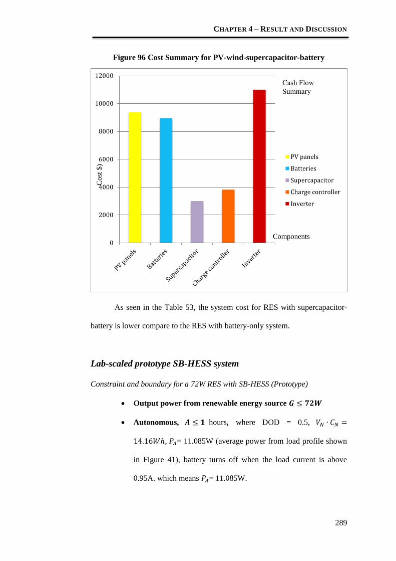
CHAPTER 4 – RESULT AND DISCUSSION
289
Figure 96 Cost Summary for PV-wind-supercapacitor-battery
As seen in the Table 53, the system cost for RES with supercapacitor-
battery is lower compare to the RES with battery-only system.
Lab-scaled prototype SB-HESS system
Constraint and boundary for a 72W RES with SB-HESS (Prototype)
Output power from renewable energy source
Autonomous, hours, where DOD = 0.5,
, = 11.085W (average power from load profile shown
in Figure 41), battery turns off when the load current is above
0.95A. which means = 11.085W.
0
2000
4000
6000
8000
10000
12000
PV panels
Batteries
Supercapacitor
Charge controller
Inverter
Co
st $
)
Cash Flow
Summary
Components

CHAPTER 4 – RESULT AND DISCUSSION
290
Expected battery lifetime , where ,
this is an estimation as this value depends on
inversion efficiency (round-trip efficiency) and also the solar
output power.
Number of supercapacitor in series, based on the
specification of the chosen supercapacitor and the DC bus voltage.
Number of 6 supercapacitors in parallel, .
Table 55 Boundary and Constraint for 72W prototype with SB-HESS
No. Components/Parameters Boundary
1 Number of PV panel, NPV 1 < NPV < 3
2 Number of batteries, NBAT 1 < NBAT < 3
3 Number of Supercapacitor, NSCAP 6 < NSCAP < 24
4 Number of Charge controller,
5 Number of Inverter, NINT NINT < 0
Table 56 Optimization Result for PV-Battery-Supercapacitor system
A
(hour)
DO
D
ybatt
(year)
No. of
battery
No. of
replacement
battery
Cost of
battery
(RM)
Net
Present
Cost
(RM)
No. of
cycles
Usable
capacity
(Wh)
1 0.5 10.1 2 2 285.3 2413 900 14.16
In the lab-scaled prototype SB-HESS, the specification of the components are
limited to run different simulation for different parameters as it is not possible
to set the different value of DOD and battery lifetime stated in the data

CHAPTER 4 – RESULT AND DISCUSSION
291
specification for our smaller scale load profile. Hence, the optimised value of
battery DOD is 0.5.
Table 57 Cost Summary for PV-Battery-Supercapacitor system
(Prototype)
Components Capital
Cost
(RM)
Replacement
Cost RM)
O&M cost
(RM)
Total (RM)
PV panels 322 0 128.8 450.8
Batteries 270 270 15.3 555.3
Supercapacitor 150 0 0 150
Charge controller 130.9 523.6 37.4 696.9
Inverter 106.61 426.44 31.95 565
System 979.51 1220.04 213.45 2413
Figure 97 Cost Summary for PV-Supercapacitor-Battery System
(Prototype)
0
100
200
300
400
500
600
700
800
PV panels
Batteries
Supercapacitor
Charge controller
Inverter
Co
st (
$)
Components
Cash Flow
Summary

CHAPTER 4 – RESULT AND DISCUSSION
292
The cost of this RES with Supercapacitor-Battery hybrid energy storage
system (SB-HESS) is reduced as compared with the cost of the conventional
PV-wind-battery system. This optimised RES with (SB-HESS) is possible
because of the energy control strategies in between these two energy storage
devices.
Generally, the overlapping of a battery’s high energy density with a
supercapacitor’s high power density produces a straightforward benefit over
either individual system by taking advantage of each characteristic. The
resulting performance is the actual fact highly related to the interconnections
and controls implemented in the system to exploit their strengths and avoid
their weaknesses. The flow coordination and energy control management for
improved energy efficiency is critical for any optimised system. There are two
main energy control management, supercapacitor-battery direct coupling
(passive control) and supercapacitor-battery indirect coupling (active control)
[51]. The direct coupling of a supercapacitor and battery energy source is where
the supercapacitor connects in parallel with batteries and load. The advantages
contributed by this simple design relative to a battery-only system include a
capability to elevate power, greater efficiency and extended battery life.
However, this design might drain the battery more as the battery tends to charge
the supercapacitors when the voltage of the supercapacitor drops (i.e. the
energy stored drops). Limitation arising from this direct coupling approach:
1. The load and supercapacitor voltages both float based on the battery
voltage that is affected by its SOC, and therefore limit exploitation of
the power capability of the supercapacitor. In addition, the requirements
of the supercapacitor module or cell voltage must match that of the

CHAPTER 4 – RESULT AND DISCUSSION
293
battery. As a result, control over the module bank size is restricted and
is hard to be optimised.
2. The power provided by the hybrid energy storage system is largely
governed by the equivalent series resistance of both coupled energy
devices. The fixed partitioning of current supply shared by
supercapacitor and battery can thus experience rippling during a pulse
demand, particularly in the battery where a magnitude of peak power is
endured at the end.
3. The terminal voltage of the HESS follows that of the battery rather than
being properly regulated; thus the voltage difference between complete
charge to discharge of a battery stack can have a significant effect on the
power provided to the load.
The optimised size of the RES is built possible with the indirect
coupling topologies active control). Indirect coupling of a supercapacitor and
battery via the addition DC-DC power converter affords a means of stepping up
or down as mentioned in Section 2.1.3.3. This approach leads HESS with
higher degrees of freedom for operation and rectifies problems and constraint
surrounding the passive direct coupling described above. Also, mentioned in
Section 1.1, the power electronics is costly, for an optimised supercapacitor-
battery HESS, our approach is to reduce the number of power electronics and in
place with a battery management system which is able to do load forecasting
using the SVM. These advantages are:
1. The supercapacitor and battery voltage can now differ from one another,
providing optimization and design flexibility.

CHAPTER 4 – RESULT AND DISCUSSION
294
2. The weight of the power source to meet peak requirement is now readily
reduced compared with passive direct coupling mentioned above.
3. A constant terminal voltage (only with small variation) can be
maintained for HESS.
4. Regulated recharging of the battery can be achieved through a DC-DC
converter without a need to introduce a charger.
5. This is also beneficial for controlling battery current supplied to the DC
bus, but the bus voltage will fluctuate according to the SOC of the
supercapacitor.
6. The safety limit of the battery is not exceeded as the microcontroller in
the system avoid the overvoltage happens in battery. At high load
currents, both the supercapacitor and battery work simultaneously.
However, the microcontroller could take action switching on battery (or
supercapacitor) base on the load forecast from SVM. It means that it
maintains the steady discharge of the battery while the supercapacitor
supplements the remaining high current.
Table 58 shows the number of batteries used in different systems. It
shows that system with hybrid energy storage system has lower number of
batteries. It is good for the environment and the cost reduction as initial cost
and replacement cost of battery has the big impact on the overall cost. Result on
optimal sizing of RES using the GA are summarised and presented in Table 59.
For a clearer comparison, RES with battery DOD 0.8 are compared and the net
present cost are presented in Table 61.
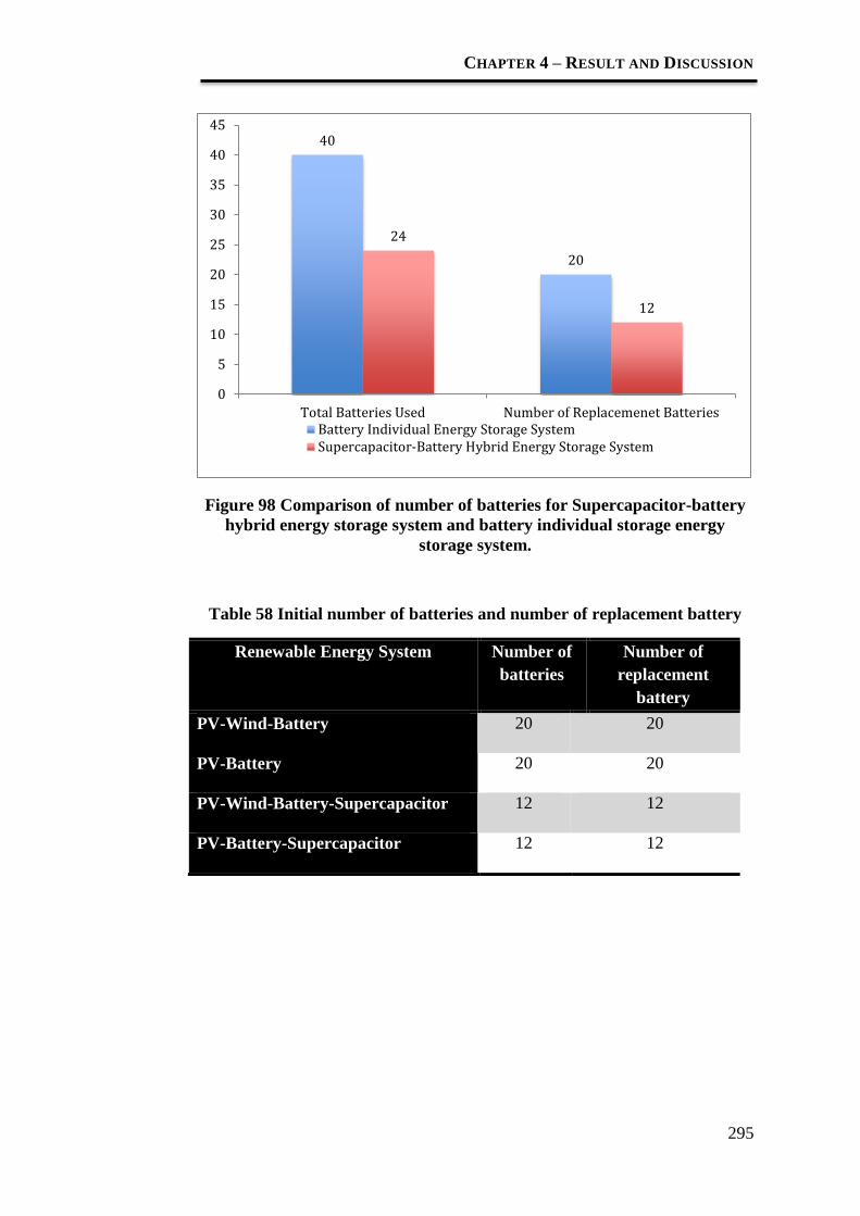
CHAPTER 4 – RESULT AND DISCUSSION
295
Figure 98 Comparison of number of batteries for Supercapacitor-battery
hybrid energy storage system and battery individual storage energy
storage system.
Table 58 Initial number of batteries and number of replacement battery
Renewable Energy System Number of
batteries
Number of
replacement
battery
PV-Wind-Battery 20 20
PV-Battery 20 20
PV-Wind-Battery-Supercapacitor 12 12
PV-Battery-Supercapacitor 12 12
40
20
24
12
0
5
10
15
20
25
30
35
40
45
Total Batteries Used Number of Replacemenet BatteriesBattery Individual Energy Storage SystemSupercapacitor-Battery Hybrid Energy Storage System

CHAPTER 4 – RESULT AND DISCUSSION
296
Table 59 Optimised Net Present Cost (NPC) of RES found using the GA
Optimised NPC of Renewable
Energy System
Cost ($) Battery lifespan
(Years)
PV-Wind-Battery LPSP = 0 LPSP =
0.1/0.2
LPSP = 0 LPSP =
0.1/0.2
43692 43692 10.3
10.3
PV-Battery 39106 39106 10.27 10.27
PV-Wind-Battery-
Supercapacitor
40723 10.4
PV-Battery-Supercapacitor 36137 10.4
Table 60 Net present cost of RES using battery DOD 0.5 found using the
GA
Renewable Energy System using
battery DOD 0.8
Cost ($) Battery lifespan
(Years)
PV-Wind-Battery 46675 12.13
PV-Battery 42089 12.13
PV-Wind-Battery-Supercapacitor 40723 10.4
PV-Battery-Supercapacitor 36137 10.4
4.2.2.3 Summary
It is apparent that the net present cost is reduced for 7.5%
by coupling the supercapacitor with battery. The main contribution of
the cost reduction is the reduction of the number of replacement
batteries throughout the 20-years of project time.

CHAPTER 4 – RESULT AND DISCUSSION
297
The implemented control strategy allows for enhanced power capacity
and reduction of battery loss are offset by the cost. It also includes
operation of the battery and supercapacitor independent voltage,
improved utilization of supercapacitor power capacity, and control of
the battery current.
Constraint plays an important role in optimization problem to be
practical in real life domain. It changes with different user specification
for that particular domain.

CHAPTER 4 – RESULT AND DISCUSSION
298
4.2.3 Energy Control Management System
One of the focuses of this project is the strategy of predicting the load
beforehand for supercapacitor-battery hybrid energy storage system (SB-
HEES). This system allows Ardrino microcontroller to control the MOSFET
switch for turning on supercapacitor before the power burst. The supercapacitor
is able to cater the entire power burst subject to zero load rejection. This allows
the battery to discharge at lower current value at a desired C-rate (discharging
rate). This aids to reduce the rate of damage mechanism of batteries by
maintaining high end-discharge voltage of the battery. Hence, a high SOC of
battery is maintained.
This section shows the reliability and the efficiency of the implemented
EMS, which is called Support Vector Machine/Regression Energy Management
System (SVMR_EMS) on the lab-scaled prototype of SB-HESS. There are
three measures of metric to prove the supercapacitor-battery hybrid energy
storage system is reliable and cost effective than conventional energy storage
system:
Section 4.2.3.1
Performance definition of the Support Vector Machine in load identification
task,
Performance definition of the Support Vector Regression in load prediction.
Section 4.2.3.2
Performance comparison between standalone battery storage and hybrid
energy storage.
Section 4.2.3.3
Performance comparison between the software approach SVMR_EMS
with the hardware approach DC/DC converter energy management system.

CHAPTER 4 – RESULT AND DISCUSSION
299
4.2.3.1 Performance definition of SVM and SVR
SVM in load Identification
The optimised load profile Classification model is trained using C-SVC type
(SVM) which is highlighted in the following:
Table 61 Performance Definition of SVM
Kernel Parameter
value
Classification
Accuracy (%)
No. of
support
Vector
Training
Time (s)
C g
Linear
2 0.25 100 24 0.005085
4 0.5 100 21 0.006105
8 0.1 100 17 0.005519
Polynomial
2 0.25 100 17 0.004866
4 0.5 100 17 0.005640
8 0.1 100 17 0.005643
Radial
Basis
Function
2 0.25 100 25 0.006726
4 0.5 100 22 0.005222
8 0.1 100 24 0.007163
Sigmoid
2 0.25 20 25 0.005024
4 0.5 20 25 0.005881
8 0.01 100 25 0.005059
From Table 61, it can be observed that the linear, polynomial and RBF
kernels with optimised function yields excellent classification accuracy. Hence,
the model with the least support vector and training time (highlighted) were
selected for better faster classification as the SVM computational complexity is
proportional to the number of support vector [286].

CHAPTER 4 – RESULT AND DISCUSSION
300
SVR in load prediction
As mentioned in Section 3.2.3. there are five simulated load profile. The
optimised regression models for each load profile were shown as the following:
Table 62 Performance Definition of SVR
Load
Profile
SVM type Kernel Parameter value MAPE
%)
Training
Time s) C g p
1
Epsilon -
SVR
polynomial 100 0.33 0.01 11.6882 0.294515
2 RBF 100 0.33 0.01 7.5650 0.018975
3 RBF 10 0.33 0.01 5.7966 0.025643
4 RBF 0.1 0.33 0.02 9.5908 0.022941
5 RBF 10 0.33 0.01 4.9574 0.020495
Table 62 shows the accuracy percentage of (MAPE) and training time
for the five simulated load profiles. A few runs of experiments were done to
select the appropriate kernel for the different load profiles and obtain the
optimised parameters value. These values and kernel type was used in the
SVM_R energy management program as shown in Appendix A4.
The predicted and actual load profiles by using the optimised models
were shown below:

CHAPTER 4 – RESULT AND DISCUSSION
301
Load
Profile
Blue = Actual load profile
Green = Predicted load profile
1
2
3
4

CHAPTER 4 – RESULT AND DISCUSSION
302
5
Figure 99 Predicted and Actual load for each load profiles
The regression model predicts the load before the actual load happens. It
is shown in the Figure 99 above. It is a feature in the energy management
system. It is important in delivering instantaneous peak power by turning on the
supercapacitor without power electronic (to build bi-directional DC-DC
converter).

CHAPTER 4 – RESULT AND DISCUSSION
303
4.2.3.2 State-of-Charge (SOC) comparison
The stress test was conducted on the lab scale battery-only system and
the hybrid system to determine the remaining battery capacity. This result
shows that the battery-only system possess the low SOC at the end of the stress
test. The SOC over load cycle graphs for each system is plotted as follows:
Figure 100 Graph of remaining battery capacity VS load cycle
As observed in Figure 100, the battery only system’s remaining capacity
has a steeper dropping gradient. On the other hand, the hybrid system’s battery
remaining capacity loss is smoother over the stress test load cycle. This has
proven that with the use of supercapacitor in the hybrid system, the battery
lifespan could be prolonged. The calculation is presented using Equation 26 and
the results are plotted in Figure 101 - 103. The calculation for plotting the graph
is shown in Appendix A5.
88
90
92
94
96
98
100
102
20 40 60 80
Rem
ain
ing
Cap
acit
y (
%)
Load Cycle Numbers
Remaining Battery Capacity
BatteryOnlySystemHybridSystem

CHAPTER 4 – RESULT AND DISCUSSION
304
Figure 101 Graph of SOC in peak load VS load cycle
Figure 102 Graph of SOC in starting up load VS load cycle
75.6
75.8
76
76.2
76.4
76.6
76.8
77
0 20 40 60 80
SO
C(%
)
Cycle Numbers
Peak Load (I=1.74)
BatteryOnlySystem
HybridSystem
75.9
76
76.1
76.2
76.3
76.4
76.5
76.6
76.7
76.8
76.9
0 20 40 60 80
SO
C(%
)
Cycle Numbers
Starting Up Load (I=1.6)
BatteryOnlySystem
HybridSystem

CHAPTER 4 – RESULT AND DISCUSSION
305
Figure 103 Graph of SOC in steady state load VS load cycle
In Figures 101, 102 and 103, the SOC of the battery in hybrid system is
observed to have smoother drop compared to the battery-only system. The
supercapacitor in the hybrid system will supply for the peak load and starting
up load; hence, the battery in hybrid system does not suffer the high rate of
discharge as much as the battery-only system. Besides, it’s also noted that the
SOC drop of the battery only system in the steady state load is higher; this is
due to the higher DOD in the battery when the battery only system is used. In
all, the supercapacitor helps to absorb the high discharge rate stress and
maintains a higher SOC level for the battery which helps to prolong the battery
lifespan.
76.72
76.74
76.76
76.78
76.8
76.82
76.84
76.86
76.88
76.9
0 20 40 60 80
SO
C(%
)
Cycle Numbers
Steady State Load (I=1.19) BatteryOnlySystemHybridSystem

CHAPTER 4 – RESULT AND DISCUSSION
306
4.2.3.3 Supercapacitor Time Response
As mentioned in Section 3.2.3, the load prediction without load profile
classification lacks of automation and is prone to erroneous results. The
following shows the supercapacitor response when the wrong load profile was
used for the load prediction:
1. SVR Load Prediction without Load Profile Identification
Actual
Load
Profile
Load Profile
Model Used
Results
Load_5
Load_2
Load_4 Load_5
Figure 104 Time Response of SVMR-EMS without load profile
identification

CHAPTER 4 – RESULT AND DISCUSSION
307
The square pulses in the diagram denote the time when supercapacitor
turns on; while the varying graph is the load current. The horizontal line shows
the peak current threshold where the supercapacitor should be turned ON when
the load current exceeds the threshold.
As seen in Figure 104, when the wrong load profile model was used for
the load prediction task, the supercapacitor was turned on either too early or too
late corresponds to the peak current threshold.
2. SVR Load Prediction with Load Profile Identification
When the load profile was identified through SVM prior to the peak load
prediction, the supercapacitor time response shows good results as shown in the
following:
No. Load
Profile
Load profile
identified
Results
1
Load_1
Load_1

CHAPTER 4 – RESULT AND DISCUSSION
308
2
Load_2
Load_2
3
Load_3
Load_3
4
Load_4
Load_4

CHAPTER 4 – RESULT AND DISCUSSION
309
Figure 105 Time Response of SVMR-EMS with load profile identification
As shown in Figure 105, the supercapacitor was turned ON before the
load current exceeds the peak current threshold. Hence, with the correct SVR
load profile model used for the regression task, the SVMR_EMS shows a good
time response as it is able to predict the peak load current and turn on the
supercapacitor in advanced for all five load profiles. Below shows the closer
looks of the load prediction results with and without load profile identification:
(a)
(b)
Figure 106 (a) Load prediction without load profile identification, (b) load
prediction with load profile identification
5
Load_5
Load_5

CHAPTER 4 – RESULT AND DISCUSSION
310
As shown in Figure 106, when the wrong load profile was used for load
prediction, the supercapacitor response lagged the peak load by 200-400ms. On
the other hand, when the load profile was successfully identified through the
SVM, the supercapacitor response leads the peak load current by 200ms as
shown in Figure 106(b). This will allows the supercapacitor to absorb the high
discharge rate stress and optimise the battery lifespan.
3. Time Response Comparison between SVMR_EMS and hardware
approach
Figure 107 SVMR_EMS and Hardware approaches’ Supercapacitor
Response
As seen in Figure 107, the hardware approach supercapacitor supplies
the load in pulsation manner. Hence, sometimes the supercapacitor response
will randomly lead and lag the peak load current demand. On the other hand,
the SVMR_EMS which predicts the peak load current in advanced will have
the supercapacitor response leading the peak load demand.

CHAPTER 4 – RESULT AND DISCUSSION
311
4. Power Efficiency of the system
The efficiencies of software approach for various loads were calculated and
plotted as follows:
Table 63 Software approach power efficiency with various loads
Load (Ω) Power Efficiency (%)
22 η =100% * (11.44 V *I) / (13 V*I) =88%
44 η =100% * (11.81 V *I) / (13 V*I) =91%
100 η =100% * (12.06 V *I) / (13 V*I) =92%
144 η =100% * (12.14 V *I) / (13 V*I) =93%
The power efficiency versus load graph was plotted as shown in the following:
Figure 108 Software approach’s power efficiency versus load
As shown in Figure 108, the software approach attains higher efficiency
when a smaller load (higher resistance) is used. This is due to the 1 Ω current
sensing resistor which formed a potential divider across the load terminal.
Hence, by increasing the load’s resistance, the voltage that supplies to the
0.87
0.88
0.89
0.9
0.91
0.92
0.93
0.94
0 20 40 60 80 100 120 140 160
Eff
icie
ncy
(%)
Load value (Ω)
Power efficiency vs load

CHAPTER 4 – RESULT AND DISCUSSION
312
terminal will increase and hence improves the power efficiency. On the other
hand, the hardware approach’s power efficiency has reported to be constant
over the range of load tested [248]. The power efficiency comparison between
the hardware approach and software approach was shown as follows:
Table 64 Comparison of power efficiency with various loads
Load Ω)
Hardware DC/DC converter
Approach efficiency (%)
Software Approach
efficiency (%)
22 93.48%
88%
44 93.48% 91%
100 93.48% 92%
144 93.48% 93%
From Table 64, it can be seen that the power efficiency of hardware
approach stays constant at 93%, while the software approach’s efficiency
increases with the load’s ohm and nearly matches the efficiency of hardware
approach when 144 ohms load is used.
5. System Cost
One of the project’s main aims is to reduce the use of expensive power
electronic through the implementation of the Software approach Energy
Management System. Hence, the itemized cost of the system were tabulated
and compared with the hardware approach as followed:

CHAPTER 4 – RESULT AND DISCUSSION
313
Table 65 SVMR-EMS system cost
Item Quantity Price
(RM)
Cost
(RM)
1. Software
Control
Board
Resistor 18 0.3~0.5 9
FQP17P10
P-channel Power
MOSFET
6 4.4 26.4
2N3904 NPN switching
Transistor
6 0.45 2.7
Terminal connector 5 0.3 1.5
Veroboard 1 3.8 3.8
1N4007 diode 0.2 3 0.6
P600K rectifier diode 3 7 21
SB560 SCHOTTKY
diode
1 0.71 0.71
1 Ω 5W current sensing
resistor
1 1 1
3 A Fuse and holder 1 1 1
Heat Sink 6 3.5 21
Arduino Mega 2560 R3 1 178 178
Total Cost 266.71
2. Hardware approach
total cost
297.11
As seen in Table 65, the hardware approach energy management system
is slightly more expensive than the software approach. The saving is significant
using software approach. The cost is reduced by 10.23% . However, the
hardware approach cost only covers for topology with discharging operation
and management of one battery cell. On the other hand, the software approach
system cost has covered the topology with full charging/ discharging operation

CHAPTER 4 – RESULT AND DISCUSSION
314
and management of multiple battery cells. Besides, unlike the hardware
approach where the DC/DC components are designed specifically for the task
requirement, the software approach offers modularity and flexibility as it could
work with a larger range of voltages. Hence, the use of software approach has
proven to be cost effective over the hardware approach.
In all, the SVMR_EMS with load prediction enables a good time
response performance that is comparable with the hardware approach. Besides
that, it could also match the power efficiency of hardware approach when
smaller load is used. Lastly, the SVMR_EMS is much more cost effective over
the hardware approach which is required the power electronics (to build the
DC-DC converter).
4.2.3.4 Analysis and Summary
Throughout this section 4.2.3.4, there are few problem faced which
could affect the reliability of the SVMR_EMS. They are listed as followed:
1. Load replicability
Since the programmable load operates by varying the opposing torque
generated by the secondary motor. The secondary motor is required to have a
constant supply of voltage and current drawn. Hence, an external DC power
supply is required to ensure the replicability of the load. Besides, the lead acid
battery voltage level varies from 12-13V as the capacity is used during the
operation. This will affect the voltage level supplied to the primary motor and
influence the load profile generated by the programmable load as seen in the
following figure:

CHAPTER 4 – RESULT AND DISCUSSION
315
(a)
b)
Figure 109 (a) Original load profile, (b) Load profile affected by Battery
voltage level drop
As seen in Figure 109(a) and Figure 109(b), the battery voltage level
drop has caused the load current profile to be lowered in magnitude. However,
due to the good generalization of the SVR, it could still predict the load pattern
when the overall load current magnitude has dropped to a certain extent. Yet, it
is required that the peak load threshold to be adjusted for the prediction to for
future work to gain 100% accuracy in all conditions.
2. Supercapacitor
Due to the lack of the voltage balancing circuit for supercapacitor, the
charging of the six supercapacitors in series might cause the imbalance
charging and discharging of the supercapacitor string. However, it added the
overall system cost. As mentioned in Chapter 1, in some cases this leads to the
use of balancing circuits, which reduce the efficacy of the supercapacitor bank.
When balancing circuits are not used (sometimes to save operational costs), the
systems runs the risk of draining the battery even more because the

CHAPTER 4 – RESULT AND DISCUSSION
316
supercapacitor will act as an additional load when its voltage is lower than the
batteries nominal voltage.
As mentioned in Chapter 1, capacitance also varies with different DC
bias voltages. Therefore, a manufactured supercapacitor, which has high
reproducibility and reliability, is important in maximizing the power reliability
of the supercapacitor after it is integrated in the power system to meet peak
power demand.
An integrated of GA-Taguchi method was applied to optimise the
process factor in supercapacitor fabrication process. Result and discussion on
this methodology step is presented in the next section.
CHAPTER 4 – RESULT AND DISCUSSION
317
4.3 Optimization of Supercapacitor fabrication process
Methodology on supercapacitor fabrication process is shown in Chapter 3.
Total of 42 supercapacitors were fabricated. In this section, performance profile
of three supercapacitors is chosen and shown in the section 4.3.1. Result shows
that the capacitance spread apart and the standard deviation is relatively large.
In the next subsection (Section 4.3.2), result and discussion on the optimization
process fabrication supercapacitor using genetic algorithm within Taguchi
signal-to-noise ratio is presented. It shows an increase in standard deviation
with the implemented Taguchi-Genetic Algorithm optimization technique on
the supercapacitors compared with the conventional Taguchi method, which
greatly involved engineering judgment.
4.3.1 Process fabrication of Supercapacitor
The test profile shown below is obtained using Autolab Potentiostat
(PGSTAT302N) under cyclic voltammetry and galvanostatic charge-discharge
tests. In chrono galvanostatic charge-discharge test, the current is set at 0.1A,
0.2A, 0.3A and 0.5A. For cyclic voltammetry, supercapacitors are tested in
different scan rate of 2mV/s, 5mV/s, 10mV/s and 20mV/s. Test profile for
three samples without any optimization technique is applied) is shown below.

CHAPTER 4 – RESULT AND DISCUSSION
318
Sample 1: Supercapacitor CS 16
1. Chrono Galvanostatic Charge-discahrge Test
Figure 110 Voltage-Time plot from Galvanostatic charge-discharge test of
Sample CS16 at different currents (0.1, 0.2, 0.3 and 0.5 A)
Figure 111 Capacitances of Sample CS16 at different currents (0.1, 0.2, 0.3
and 0.5 A)
-0.5
0
0.5
1
1.5
2
2.5
0 100 200 300 400 500 600 700
Vo
lta
ge
(V
)
0.1A
0.2A
0.3A
0.5A
Time (s)
0
50
100
150
200
250
0 0.1 0.2 0.3 0.4 0.5 0.6
Ca
pa
cita
nce
(F
)
Current (A)
225.0 221.00
69.06
36.49

CHAPTER 4 – RESULT AND DISCUSSION
319
2. Cyclic Voltammetry
Figure 112 Cyclic Voltammograms at various scan rates (2, 5, 10, 20mV/s)
Figure 113 Capacitance plots of Sample CS16 at various scan rate (2, 5, 10,
20mV/s)
-5.00E-01
-4.00E-01
-3.00E-01
-2.00E-01
-1.00E-01
0.00E+00
1.00E-01
2.00E-01
3.00E-01
4.00E-01
5.00E-01
6.00E-01
0 0.5 1 1.5 2 2.5
2mV/s
5mV/s
10mV/s
20mV/s
Current
Voltage (V)
-4.00E+01
-3.00E+01
-2.00E+01
-1.00E+01
0.00E+00
1.00E+01
2.00E+01
3.00E+01
4.00E+01
5.00E+01
0 0.5 1 1.5 2 2.5
2mV/s
5mV/s
10mV/s
20mV/s
Voltage (V)
Capacitance (F)

CHAPTER 4 – RESULT AND DISCUSSION
320
Figure 114 Overall capacitance of Sample CS16 at different scan rate (2, 5,
10, 20mV/s)
Sample 2:
Supercapacitor CS 33
1. Chrono Galvanostatic Charge-discahrge Test
Figure 115 Voltage-time plot from galvanostatic charge-discharge test of
Sample CS33 at different currents (0.1, 0.2, 0.3 and 0.5 A)
0
5
10
15
20
25
30
0 5 10 15 20 25Scan Rate (mV/s)
Ca
pa
cita
nce
(F
) 25.11
23.53
18.40
14.11
-0.5
0
0.5
1
1.5
2
2.5
0 100 200 300 400 500
0.1A
0.2A
0.3A
0.5A
Time (s)
Vo
lta
ge
(V
)
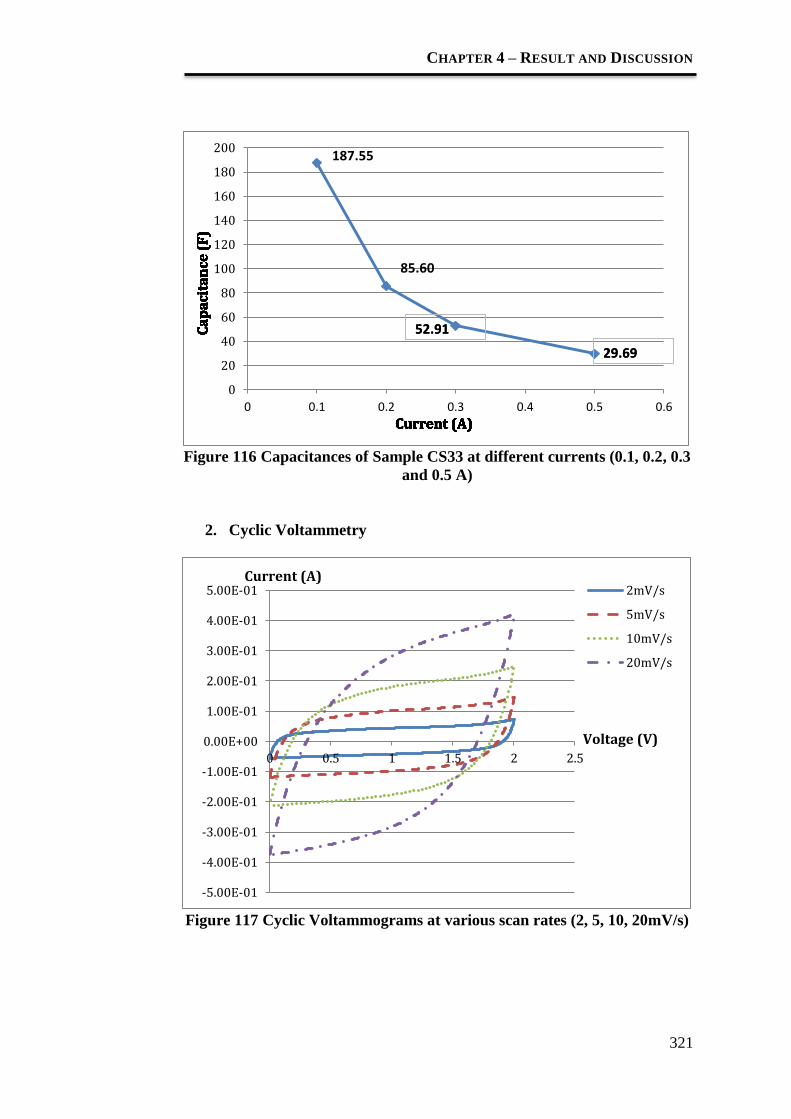
CHAPTER 4 – RESULT AND DISCUSSION
321
Figure 116 Capacitances of Sample CS33 at different currents (0.1, 0.2, 0.3
and 0.5 A)
2. Cyclic Voltammetry
Figure 117 Cyclic Voltammograms at various scan rates (2, 5, 10, 20mV/s)
0
20
40
60
80
100
120
140
160
180
200
0 0.1 0.2 0.3 0.4 0.5 0.6
Current (A)
Ca
pa
cita
nce
(F
)
52.91
29.69
Current (A)
Ca
pa
cita
nce
(F
)
52.91
29.69
Current (A)
Ca
pa
cita
nce
(F
)
Current (A)
Ca
pa
cita
nce
(F
)
Current (A)
Ca
pa
cita
nce
(F
)
Current (A)
Ca
pa
cita
nce
(F
)
Current (A)
Ca
pa
cita
nce
(F
)
Current (A)
Ca
pa
cita
nce
(F
)
Current (A)
Ca
pa
cita
nce
(F
)
Current (A)
Ca
pa
cita
nce
(F
)
Current (A)
Ca
pa
cita
nce
(F
)
Current (A)
Ca
pa
cita
nce
(F
)
Current (A)
Ca
pa
cita
nce
(F
)
187.55
85.60
-5.00E-01
-4.00E-01
-3.00E-01
-2.00E-01
-1.00E-01
0.00E+00
1.00E-01
2.00E-01
3.00E-01
4.00E-01
5.00E-01
0 0.5 1 1.5 2 2.5
2mV/s
5mV/s
10mV/s
20mV/s
Current (A)
Voltage (V)

CHAPTER 4 – RESULT AND DISCUSSION
322
Figure 118 Capacitance plots of Sample CS33 at various scan rates (2, 5,
10, 20mV/s)
Figure 119 Overall capacitance of Sample CS33 at different scan rates (2,
5, 10, 20mV/s)
-4.00E+01
-3.00E+01
-2.00E+01
-1.00E+01
0.00E+00
1.00E+01
2.00E+01
3.00E+01
4.00E+01
5.00E+01
0 0.5 1 1.5 2 2.5
2mV/s
5mV/s
10mV/s
20mV/s
Voltage (V)
Capacitance (F)
0
5
10
15
20
25
0 5 10 15 20 25
20.64
18.41 16.10
Scan Rate (mV/s)
Ca
pa
cita
nce
(F
)
13.01

CHAPTER 4 – RESULT AND DISCUSSION
323
Sample 3:
Supercapacitor CS 34
1. Chrono Galvanostatic Charge-discahrge Test
Figure 120 Voltage-time plot from galvanostatic charge-discharge test of
Sample CS34 at different currents (0.1, 0.2, 0.3 and 0.5 A)
Figure 121 Capacitances of Sample CS34 at different currents (0.1, 0.2, 0.3
and 0.5 A)
-0.5
0
0.5
1
1.5
2
2.5
0 200 400 600 800
0.1A
0.2A
0.3A
0.5A
Vo
lta
ge
(V
)
Time (s)
0
50
100
150
200
250
0 0.1 0.2 0.3 0.4 0.5 0.6
Current (A)
Ca
pa
cita
nce
(F
)
215.24
99.94
64.00
33.38

CHAPTER 4 – RESULT AND DISCUSSION
324
2. Cyclic Voltammetry
Figure 122 Cyclic Voltammograms at various scan rates (2, 5, 10, 20mV/s)
Figure 123 Capacitance plots of Sample CS34 at various scan rate (2, 5, 10,
20mV/s)
-5.00E-01
-4.00E-01
-3.00E-01
-2.00E-01
-1.00E-01
0.00E+00
1.00E-01
2.00E-01
3.00E-01
4.00E-01
5.00E-01
0 0.5 1 1.5 2 2.5
2mV/s
5mV/s
10mV/s
20mV/s
Current (A)
Voltage (V)
-4.00E+01
-3.00E+01
-2.00E+01
-1.00E+01
0.00E+00
1.00E+01
2.00E+01
3.00E+01
4.00E+01
5.00E+01
0 0.5 1 1.5 2 2.5
2mV/s
5mV/s
10mV/s
20mV/s
Voltage (V)
Capacitance (F)

CHAPTER 4 – RESULT AND DISCUSSION
325
Figure 124 Overall capacitance of Sample CS34 at different scan rates (2,
5, 10, 20mV/s)
4.3.2 Summary and analysis
The graphs above are summarised and explained here. Value of
capacitance for the three samples shown above is summarised in the figure and
table below. The capacitance obtained from CV and charge-discharge test
profiles shown previously is inconsistent. From observation, the curves in
charge-discharge testing does not start from zero volts and consistently started
from around 0.5V. This is due to the pre-treatment was not done correctly, for
example, the supercapacitor was not discharge to zero completely before
glavonastic charge-discharge test begins.
0
5
10
15
20
25
30
0 5 10 15 20 25Scan Rate (mV/s)
Ca
pa
cita
nce
(F
)
23.85
20.60
17.58
13.64

CHAPTER 4 – RESULT AND DISCUSSION
326
Figure 125 Capacitance for Supercapacitor Samples at different scan rates
Table 66 Capacitance for Supercapacitors at different scan rate
Supercapacitor Capacitance at different scan rate
2mV/s 5mV/s 10mV/s 20mV/s
CS16 25.11 23.53 18.40 14.11
CS33 20.64 18.41 16.10 13.01
CS34 23.85 20.60 17.58 13.64
Table 67 Capacitance for Supercapacitors at different current
Supercapacitor Capacitance at different current
(F)
0.1A 0.2A 0.3A 0.5A
CS16 225.0 221.0 69.06 36.49
CS33 187.55 85.60 52.91 29.69
CS34 215.24 99.94 64.00 33.38
Table 67 above shows the capacitance of the supercapacitors at different
scan rate. From the equation shown in Section 3.3.1,
Equation 44
0
5
10
15
20
25
30
0 5 10 15 20 25
CS16
CS33
CS34Cap
acit
ance
(F)
Scan Rate (mV/s)

CHAPTER 4 – RESULT AND DISCUSSION
327
where is C the capacitance, I the applied electric current and
s is the scan rate.
Based on the Figure 125 and Table 66, it can be said that decreasing the
sweep rate results in increasing the total capacitance of the supercapacitor.
Lowering the sweep rates allows more amount of time for the ions to access the
bulk of holes on the active material.
More importantly, from the profile shown above, the capacitance values
going down the table is not consistent. By comparing readings for the same
settings of the test procedure, the capacitance value spread over a wide range
within the same scan rate shown in Table 66 and 67. We reckon that the
supercapacitor fabrication process can be optimised to obtain smaller standard
deviation for capacitance. To ensure a robust process, a novel optimization
technique is introduced in the next section. The novelty consists of including a
genetic algorithm within the Taguchi technique to optimise the normalised
signal-to-noise ratio of the process for multiple output response. It proves that
the capacitance and ESR are closer to the target value with the implemented
strategy.

CHAPTER 4 – RESULT AND DISCUSSION
328
4.3.2 Optimization of process factors in Supercapacitor
fabrication using the Genetic Algorithm within Taguchi
Signal-to-Noise ratios
As mentioned in Section 3.3.2, L4 is used for DOE orthogonal array. All the
trials were conducted and the results are shown in the Table 68. Three samples
were produced for each run (experiment with the same setting of low and high
level). The capacitance and ESR performance for the samples were tested using
an Autolab Potentiostat (PGSTAT302N) under cyclic voltammetry and
galvanostatic charge-discharge tests respectively. Table 69 summarizes the
transformation values of raw data from the Table 68 into SNR and Z. Response
1 – capacitance (Farad, F) is calculated using Equation 66 while response 2
ESR (Ohm, Ω) is calculated using Equation 67 below. The calculation is based
on the CV curve and Charge-discharge curve tested using Autolab. These
testing profiles are shown in Appendix A6. Calculation is done using the
Equation below. It is shown in Appendix A6.
( ( ( )
( )
Equation 66

CHAPTER 4 – RESULT AND DISCUSSION
329
Figure 126 Charge and Discharge Curve
Table 68 Experimental output data
The equivalent series resistance, ESR value can be determined by using the
following equation and the calculation and test profile are shown in Appendix
A6.
ESR (Ω) = ( )
( ) Equation 67
Process Experiment, i (yc)n - Capacitance (F) (yE)n - ESR (Ω)
Sample
1
Sample
2
Sample
3
Sample
1
Sample
2
Sample
3
1
Mixing
1
2
3
4
0.989
1.942
2.231
1.624
1.074
2.070
2.441
1.675
1.105
2.074
2.399
1.820
12.15
12.80
3.20
9.05
19.05
4.70
6.60
17.45
18.45
14.15
2.00
11.20
2
Calendaring
1
2
3
4
2.035
2.583
1.967
2.140
2.039
2.440
1.901
2.173
2.132
2.654
1.979
2.406
2.30
2.35
2.85
2.25
3.50
2.05
2.06
3.00
3.15
3.20
2.35
2.95
3
Drying
1
2
3
4
2.295
2.558
2.681
2.448
2.462
2.317
2.338
2.581
2.409
2.680
2.578
2.459
2.85
2.30
2.70
2.45
2.50
2.90
2.95
2.50
2.55
2.75
2.30
2.70
4
Electrolyte
Treatment
1
2
3
4
1.757
2.457
1.622
2.293
1.901
2.590
1.598
2.556
1.653
2.468
1.605
2.558
3.35
2.56
5.10
2.40
2.85
2.61
6.45
2.50
3.00
2.81
4.25
2.30

CHAPTER 4 – RESULT AND DISCUSSION
330
Table 69 shows the values for signal-to-noise ratio for capacitance and ESR
output responses ((SNR)ic and (SNR)iE ). Response 1 – capacitance (Farad, F) is
calculated using Equation 68 while response 2 ESR (Ohm, Ω) is calculated
using Equation 69. For a clearer view, an example is shown below to illustrate
how the values are obtained.
\
For experiment, i=1 in mixing process,
SNR for the capacitance response (larger-the-better)
SNiC = -10 ( )∑
SN1C
(
[
( ) ( )
( ) ]
(
[
( ) ( ) ( ) ])
Equation 68
SNR for the ESR response (smaller-the-better)
SNiE = -10 ( )∑
SN1E
(
[( )
( ) ( )
]
(
[( ) ( ) ( ) ])
Equation 69

CHAPTER 4 – RESULT AND DISCUSSION
331
where yi is the experimental data at the ith sample and n is the
number of samples.
In Table 69, the negative on the SNR for the ESR response indicates
that the smaller-the-better for this output response.
Table 69 Weighted SNR (WSNR) Values
Output response for capacitance and ESR are also used to calculate
normalised SNR for the implemented GA fitness function to find the optimal
weights for each process. This is important to see which process factor has the
Process Experiment, i (SNR)ic (SNR)iE Zic ZiE WSNRi
1
Mixing
1
2
3
4
10.03
15.69
16.99
14.19
-24.53
-21.22
-12.85
-22.32
0.578
0.656
0.600
0.420
0.362
0.393
0.580
0.581
0.5778
0.6557
0.5998
0.4202
2
Calendaring
1
2
3
4
15.85
17.71
15.34
16.56
-9.62
-8.23
-7.75
-8.80
0.3471
0.5561
0.6154
0.3747
0.4306
0.3333
0.5443
0.3556
0.3484
0.5526
0.6143
0.3744
3
Drying
1
2
3
4
17.11
17.58
17.63
17.45
-8.43
-8.50
-8.51
-8.14
0.5609
0.5546
0.5666
0.3609
0.6190
0.4167
0.4615
0.6000
0.5612
0.5539
0.5661
0.3621
4
Electrolyte
Treatment
1
2
3
4
14.52
17.52
13.67
16.34
-9.75
-8.50
-14.55
-7.61
0.4731
0.3609
0.4306
0.6642
0.5667
0.6000
0.5379
0.5000
0.5649
0.5953
0.5358
0.5032

CHAPTER 4 – RESULT AND DISCUSSION
332
most influence to that particular process. Transformation SNR to normalised
SNR (Zic and ZiE) is done using Equation 70 and Equation 71. For mixing
process and first experiment, the working is shown below:
Normalised SNR for the capacitance response (the-larger-the-
better) [13];
= ( ) )
= ( ) )
Where Yavg = is the average out of the n number of samples
produced, Yavg
and are the least and highest data
value out of the n number of samples produced respectively.
Equation 70
Normalised SNR for the ESR response (the-smaller-the-better)
[13];
= ( ) )
( ) ( )
where Yavg is the average out of the n number of samples
produced, Yavg
Ymin =12.15 and Ymax = 19.05 are the least and highest data
value out of the n number of samples produced respectively.
Equation 71
These normalised SNR (Zic and ZiE ) values are used for GA fitness function
(Equation 72). By applying the implemented GA fitness function to the GA

CHAPTER 4 – RESULT AND DISCUSSION
333
programming, the optimal weight of wc and wE are found to determine the
weighted normalised SNR, WSNR. Optimal weights for each response are
obtained using the GA. From the GA simulation, weights for each process are
maximized with the calculated SN ratio as shown in Table 69.
For example, in Process 1, wc and wE were found to be 0.9990 and
0.0001 respectively. From the GA simulation, the optimal weights are [0.9990,
0.0001].
F(x) = ∑ ∑ ( )
( ) ( ) (
)
Equation 72
The objective of this algorithm is to find the optimal weights so as to
maximize the normalised SNR. Therefore, at the maximum point in the GA
simulation, wc and wE were obtained and shown in Table 70.
Table 70 Optimal wc and wE
Process wC wE
1 0.9990 0.0001
2 0.9844 0.0156
3 0.9951 0.0049
4 0.0196 0.9804
To determine the value of WSNRi which is shown in Table 70:
For mixing process, experiment i = 1, optimal weights were obtained early is
used to calculate the value WSNRi.
WSNRi = wc ZiC + wE ZiE
WSNR1 = 0.999Z1C + 0.0001Z1E
WSNR1 = 0.999 *(0.578) + 0.0001 * (0.362)
= 0.577

CHAPTER 4 – RESULT AND DISCUSSION
334
WSNR values for each trial and each process were computed (by
substituting the wC and wE values into the WSNR formula as shown above), it
was noticed that in Process 1 (mixing), experiment 2 (run 2) has the highest
WSNR value. If we refer back to Table 35, it corresponds to A1, B2, C2 as the
desired setting for the Process 1. However, this approach is less accurate as the
interactions between factors and levels have not yet been taken into account.
The same can be implied for the rest of the processes (Process 2, 3 and 4). A
better approach is shown to evaluate the main effects on WSNR for each
process factor using Equation 58, 59, 60, 61, 62 and 63 were performed to
obtain the average WSNR. For example, for mixing process, for factor A1, L1
and L2 (which is shown in Table 71) are calculated using Equation 58 and
Equation 59:
low level, L1 = (WSNR1+ WSNR2) / 2
= (0.5778 + 0.6557) / 2
= 0.6167 where WSNR1 and WSNR2 are taken from Table 69.
However,
for high level, L2 = (WSNR3+ WSNR4) / 2
= (0.59998 + 0.4202) / 2
= 0.510 where WSNR1 and WSNR2 are taken from Table 69.
This average WSNR values indicates the effect on the low and the high
level for each factor. The higher the difference between the minimum (factor at
low level) and maximum (factor at high level) is, the greater the effect it will
have. Hence, in Table 71, (WSNRmax -WSNRmin) provides the details of the
main effects on WSNR. Figure 127 consists of four sets of the main effect plot
for the respective process fabrication. This is a way to illustrate the information

CHAPTER 4 – RESULT AND DISCUSSION
335
obtained from Table 71. It provides the predicted optimal conditions for the
process optimization. For Process 1, the optimal condition predicted is A1, B1,
C2 as for having higher WSNR values. Process 2 on the other hand is A2, B1, C2
while Process 3 is A1, B1, C2 and Process 4 is also A1, B1, C2. An observation
that can be seen is that Factor C (machine temperature) in Process 2
(calendaring) has the biggest margin with 0.2221 differences of its two levels.
This tells us that such factor is quite sensitive if we change the level values thus
it is a significant factor in producing a good quality of process or product. On
the other hand, the very small margin of 0.0011 obtained in Process 4
(electrolyte treatment) and Factor B (molarity) indicates that such factor does
not have much effect on the outcome if we change the level values. In a later
section, a more appropriate way for determining significant and insignificant
factors using ANOVA will be discussed.
Table 71 Main Effects on WSNR for every factor investigated of the
respective process
Process Factors Low
Level,
L1
High
Level,
L2
WSNRmax -WSNRmin
1
Mixing
A Mixing Speed
B Mixing Time
C Amount of AC
0.6167
0.5889
0.4990
0.5101
0.5379
0.6278
0.1066
0.0509
0.1288
2
Calendaring
A Calendaring time
B Thickness
C Machine temp.
0.4505
0.4813
0.3614
0.4943
0.4635
0.5835
0.0438
0.0178
0.2221
3
Drying
A Heating time
B Heating temp.
C Vacuum
0.5575
0.5636
0.4617
0.4641
0.4580
0.5600
0.0934
0.1057
0.0984
4
Electrolyte
Treatment
A Electrolyte name
B Electrolyte molarity
C Electrolyte amount
0.5801
0.5504
0.5340
0.5195
0.5493
0.5656
0.0606
0.0011
0.0315

CHAPTER 4 – RESULT AND DISCUSSION
336
a.P1- (mixing) b.P2-(calendaring)
c.P3-(drying) d.P4-(electrolyte treatment)
Figure 127 Factor effects on WSNR
Confirmation experiment
In confirmation of the predicted optimal settings obtained from the proposed
Taguchi-GA approach, verification tests were conducted and another three
samples were each produced and the results obtained are tabulated in Table 72.
To evaluate the findings, a comparison of the standard deviation (SD) for all of
the trials is conducted. The smaller value of SD implies the consistency of the
samples and thus indicates that they are close to the target value. Consistency is
related to process repeatability and robustness of product.
WS
NR
Va
lue
s
Factor Levels
WS
NR
Va
lue
s
Factor Levels
WS
NR
Va
lue
s
Factor Levels
WS
NR
Va
lue
s
Factor Levels

CHAPTER 4 – RESULT AND DISCUSSION
337
Table 72 Experimental output data for confirmation experiments
Process Output Response
Sample 1 Sample 2 Sample 3
P1-Mixing
(A1, B1, C2)
2.425 F; 1.602 Ω 2.388 F; 3.691 Ω 2.403 F; 2.925 Ω
P2-Calendaring
(A2, B1, C2)
2.051 F; 1.811 Ω 2.026 F; 2.008 Ω 2.095 F; 1.760 Ω
P3-drying
(A1, B1, C2)
2.294 F; 2.571 Ω 2.310 F; 2.529 Ω 2.244 F; 2.708 Ω
P4-electrolyte treatment
(A1, B1, C2)
2.199 F; 1.98 Ω 2.222 F; 1.85 Ω 2.213 F; 2.00 Ω
The standard deviations (SD) were obtained using the following formula;
SD = √ ∑( ) ∑ )
)
where N is the number of replication and X is the experimental
data.
Equation 73
Table 73 SD for each experiment and under optimal conditions
Process Experiment, i SD
(capacitance)
SD (ESR)
1 1
2
3
4
5 (A1, B1, C2)
0.0601
0.0751
0.1766
0.1111
0.0186
3.8223
5.1110
2.3861
4.3636
1.0568
2 1
2
3
4
5 (A2, B1, C2)
0.0549
0.1090
0.0420
0.1445
0.0349
0.6171
0.5965
0.3996
0.4193
0.1310
3 1
2
3
4
5 (A1, B1, C2)
0.0853
0.1847
0.1760
0.0738
0.0650
0.1893
0.3122
0.3279
0.1323
0.0936
4 1
2
3
4
5 (A1, B1, C2)
0.1245
0.0738
0.0123
0.1524
0.0116
0.2566
0.1323
0.1094
0.1000
0.0814

CHAPTER 4 – RESULT AND DISCUSSION
338
Table 73 shows that the predicted condition in every process yields a
certain extent of improvement of capacitance and ESR standard deviation.
Standard deviation for experiments 1 – 4 in Table 73 are the standard deviation
before the process is optimised using Taguchi-GA method, whereas,
experiment 5 is the standard deviation result after Taguchi-Ga method was
applied. Overall, the standard deviation is improved. Such findings proved that
the novel Taguchi-GA have successfully optimised the weighs and has thus
maximized the values of SN ratio for both responses.
The SNRs for the initial condition are obtained by assigning 0.7
weighting for the capacitance response and 0.3 for the ESR response arbitrarily,
based on the consensus that the capacitance performance should dominate the
ESR response before conducting the GA approach. The GA method then
searches for the optimal weightings that maximize the SNR for both responses
to improve the performance of process factors. Refer to the outcome in thesis
[287], experiments for few different value of OEC were carried out and
different capacitance to ESR ratio (combinations total = 1) have also been
tested - 0.6:0.4, 0.2:0.8 etc. It was found that after the capacitance ratio being
altered gradually for example 0.2, 0.3, 0.4 etc, the outcome results in the same
experimental run (e.g. Run 2) as the best run for the respective process.
However, until at a certain ratio (e.g 0.8:0.2) the results turn up to give a
different experimental run (e.g. Run 3) as the best run. This shows that the
weight has certain impact on the optimal setting to be predicted. If that is so,
there is a chance to fully optimise the SNR. This can be done without using
engineering judgment.

CHAPTER 4 – RESULT AND DISCUSSION
339
For this case study, only one weight ratio of 0.7:0.3, was used for the
OEC computation and comparison after considered that this OEC value has
higher SNR value (shown in [287]). This is treated as the initial condition. It is
compared with the WSNR obtained using the integrated Taguchi and GA
method in the later part.
Table 74 OEC values to determine the optimal setting for the initial
condition
Process Experiment, i Combination OEC (0.7:0.3 weighting)
1 1
2
3
4
A1, B1, C1
A1, B2, C2
A2, B1, C2
A2, B2, C1
0.5125
0.5756
0.5940
0.4669
2 1
2
3
4
A1, B1, C1
A1, B2, C2
A2, B1, C2
A2, B2, C1
0.3754
0.5641
0.5941
0.3112
3 1
2
3
4
A1, B1, C1
A1, B2, C2
A2, B1, C2
A2, B2, C1
5.8250
5.1260
5.3430
4.3260
4 1
2
3
4
A1, B1, C1
A1, B2, C2
A2, B1, C2
A2, B2, C1
0.5012
0.2526
0.4628
0.6149
The overall improvement percentage is determined as the ratio between
sums of the improvement values of all responses for the confirmation
experiment (after optimised using Taguchi-GA method) and the sum of the
SNRs of initial responses for all responses. Using the method shown in [256],
this is called the addictive model. It is used to predict the anticipated
improvements under the chosen optimum conditions (optimal level of the
process factor); the SNRs for these two output responses are predicted and

CHAPTER 4 – RESULT AND DISCUSSION
340
shown in Table 75 (last column, improvement). For a clearer view, taking
Process 1 (mixing) as an example,
( )
( )
( )
( )
( )
( )

CHAPTER 4 – RESULT AND DISCUSSION
341
Table 75 Initial, predicted and actual improvement of SN ratio
* The setting combination for process level is obtained from OEC (overall
evaluation criteria) computation (0.7:0.3) shown in Table 74, which the highest
OEC is chosen for the optimum level for the process factor.
** The setting combination for process level is predicted using the highest
WSNR given in Table 69. For example, in process 1 (mixing), the highest WSN
value is at run 2 (experiment 2), hence, SNR for predicted setting combination
for the process level is 15.69 for capacitance and -21.22 for ESR which are
taken in Table 69 (the italic value).
***By using the output responses shown in Table 68 and apply the values to
Equation 67 and Equation 68, the SNR values are calculated for the
confirmation experiment (after optimised using Taguchi-GA method).
Table 75 presents how the combination of the initial condition is made
by selecting the highest OEC values in every fabrication process. The SNRs of
Process Responses Initial
condition
(dB)
Predicted
condition (GA)
(dB)
Confirmation
(dB)
Improvement
(dB)
1 SNRc 16.99 15.69 17.166 0.176
SNRE -12.85 -21.22 -9.164 3.686
Optimal setting A2, B1, C2* A1, B2, C2**
A1, B1, C2***
Overall improvement
in (dB %)
12.9 %
2 SNRc 15.34 15.34 15.340 0.000
SNRE -7.75 -7.75 -5.798 1.952
Optimal setting A2, B1, C2* A2, B1, C2**
A2, B1, C2***
Overall improvement
in (dB %)
8.4 %
3 SNRc 17.11 17.63 17.18 0.07
SNRE -8.43 -8.51 -8.31 0.12
Optimal setting A1, B1, C1* A2, B1, C2**
A1, B1, C2***
Overall improvement
in (dB %)
0.7 %
4 SNRc 16.34 17.52 16.44 0.10
SNRE -7.61 -8.50 -5.78 1.83
Optimal setting A2, B2, C1* A2, B1, C2**
A1, B1, C2***
Overall improvement
in (dB %)
8.1 %

CHAPTER 4 – RESULT AND DISCUSSION
342
those experimental runs that based on the processing parameters as in Table 75
are compared with the SNRs of the experiments which use WSNR values
shown in Table 69. In Table 75, it is observed that 12.9%, 8.4% and 8.1%
improvement in dB was obtained for the mixing, calendaring and electrolyte
treatment process respectively by using the proposed Taguchi-GA approach.
However, the drying process does not produce much improvement (0.7% only).
One possible reason for this small improvement is that the optimization has
reached its certain limit for given factors and levels assigned. Unless different
factors are added in to be investigated, this could further improve the process.
The purpose of ANOVA in this study is to determine which of the
process factors are significantly affect the performance characteristics [256] in
the supercapacitor fabrication. To achieve this, the total variability of the multi-
objective WSNR measured by the sum of squared deviations is separated from
the total mean of WSNR, before converting into percentage contribution for
every individual factor. This part was implemented by utilizing the Qualitek-4
software. Some of the factors are pooled to avoid calling something significant
when it is not. This is to maximize the percentage contribution of the dominant
and significant factors. Table 76 displays the ANOVA results.

CHAPTER 4 – RESULT AND DISCUSSION
343
Table 76 Results of ANOVA analysis on WSNR
Process Factor DOF Sum of Squares % Contribution
1 A
B
C
Error
Total
1
1
1
0
3
0.011
0.002
0.016
0.030
37.181
8.360
54.130
100 %
2 A
B
C
Error
Total
1
(1)
1
1
3
0.001
(0)
0.049
-0.01
0.051
3.16
POOLED
96.00
0.84
100 %
3 A
B
C
Error
Total
1
1
1
0
3
0.008
0.011
0.009
0.029
29.230
37.973
32.458
100 %
4 A
B
C
Error
Total
1
(1)
1
1
3
0.003
(0)
0.001
-0.001
0.004
91.503
POOLED
24.803
-16.306
100 %
Consequently, optimal conditions for every process can be set as A1, B1,
C2 for the mixing process, A2, B1, C2 for the calendaring process, A1, B1, C2 for
the drying process, and A1, B1, C2 for the electrolyte process. It is found that the
most significant process factor for the respective process is in the sequence of
machine temperature (96%) in the calendaring process, followed by the KCl
electrolyte (91.503%) in the electrolyte treatment process, the amount of
activated carbon (54.13%) in the mixing process, and finally the heating
temperature (37.97%) in the drying process. Such process factors with a high
percentage contribution obtained statistically are believed to have a huge impact
towards the performance of the supercapacitor fabricated and outcome shown in
Table 76 is good for future improvement where process factors that has low
percentage contribution can be eliminated.

CHAPTER 4 – RESULT AND DISCUSSION
344
4.3.2.1 Summary
The supercapacitor fabrication process dealing with a multi response problem
has been presented. From the experimental and analytical results, the
conclusions are as follows:
Taguchi method has successfully minimised the cost and time span of the
experimental procedure consisting of three factors and two-level each.
Only four trials are required when using the orthogonal array experiment.
The proposed integrated approach has improved the SNR (dB) as shown in
the Figure 128 below. Hence, optimal conditions have great influences on
the design factors with less sensitivity to the noise factors.
Figure 128 Percentage of SNR improvement after optimization as
compared to using OEC method
The proposed Taguchi-GA integrated strategy provides a robust design
in the sense of reproducibility and reliability. This could not be achieved
by the OEC approach alone as this approach is dependent on
engineering judgment that has higher variation, a mean value that is far
from the desired target value if those judgments were inaccurately
made. The figure below shows that the standard deviation for both

CHAPTER 4 – RESULT AND DISCUSSION
345
output response (Capacitance and ESR) is improved as compared with
the conventional method (Taguchi and OED method).
Figure 129 Standard deviation comparison before & after optimisation
(Capacitance)
Figure 130 Standard deviation comparison before & after optimisation
(ESR)
The optimum process setting ensures optimum values for capacitance
and ESR. By applying the optimum process setting (process condition),
consistent capacitance and ESR values of supercapacitors are
0
0.02
0.04
0.06
0.08
0.1
0.12
0.14
mixing calendering drying electrolyte t.
SD before
SD after
0
0.5
1
1.5
2
2.5
3
3.5
4
4.5
mixing calendering drying electrolyte t.
SD before
SD after

CHAPTER 4 – RESULT AND DISCUSSION
346
guaranteed as shown in the lower standard deviation values as compared
to the standard deviation for the samples which were not applied
Taguchi-GA optimisation method. This is important for the optimised
supercapacitor-battery hybrid energy storage system. This is to ensure
power reliability of the system.

CHAPTER 5 – CONCLUSION
347
CHAPTER 5
CONCLUSION
This project dealt with the integration of supercapacitors into a battery energy
storage system for solar applications in order to optimise overall cost by
prolonging battery lifespan utilizing the Genetic Algorithm (GA) and Support
Vector Machine (SVM) further reliability was optimised by using Genetic
Algorithm within the Taguchi technique to reduce spread in tolerance of
supercapacitors values which affect system performance.
The main achievement in this research is to minimise operational cost of
a solar system by integrating supercapacitors into a hybrid lead acid battery
energy management system. It has been accomplished as described in Table 77.
This project sought to investigate and solve the research issues arising from
combining supercapacitors with batteries in a hybrid energy system which is
then made economically feasible thru process and operational optimization.
This was done using a GA and a supervised learning machine – Support Vector
Machine (SVM) to in place of costly power electronics (dc-dc converter). The
general literature review on this subject and specifically in this context of
optimising the supercapacitor-battery hybrid energy storage system in solar
application is inconclusive on several vital research issues on pairing the
supercapacitor and battery in an energy storage system. Simulation and
optimization on model which involves supercapacitor could not be done in most
of the commercial optimization software such as HOMER, HYBRID and etc.
However, in this project, the implemented fitness function in GA has

CHAPTER 5 – CONCLUSION
348
successfully optimised the cost of the Supercapacitor-battery hybrid energy
storage system by reducing the rate of battery damage mechanism.
It is also interesting to state that the overall cost of the implemented SB-
HESS was further optimised by applying SVM and SVR (Support Vector
Regression) within the energy management system which accurately predicts
the load demand in advance. This was done by replacing part of the power
electronics with intelligent software which allows the improvement of
efficiency and lowers the cost of other components such as in eliminating the
need for a bi-directional dc-dc converter used in balancing the voltage level
between supercapacitor and battery. This is very crucial to make sure that the
systems does not run the risk of draining the battery due to the supercapacitor
acting as an additional load if its voltage is lower than the batteries nominal
voltage as both energy storage devices are in direct parallel connection.
This implemented system is more cost effective as it is integrated with
the wide availability and affordability of microcontrollers which allows these
hybrid systems to be controlled using purely software methods such as by
employing the Support Vector Machine (SVM) pattern classifier to decide
when to switch energy sources depending on the load requirement. This
supervised learning system was used to predict load demand before it occurs. It
is proven that aids in reducing the delay in delivering power even when there
are a few possibilities to be considered in connecting or disconnecting battery
and supercapacitor to the load. This not only lowers the operational cost, but at
the same time, allows the hybrid photovoltaic system to be flexible, which
comes in handy in places with different seasons and unpredictable weather. The
implementation using a microcontroller also allows the monitoring of multiple

CHAPTER 5 – CONCLUSION
349
parameters, which may affect the efficiency of the hybrid photovoltaic systems,
optimising the operation of these systems by taking appropriate actions when
needed.
The cost of the implemented system i.e the supercapacitor-battery
hybrid energy storage system (SB-HESS) is reduced by approximately 7.51%
compared to the conventional individual battery energy storage system. In SB-
HESS, the number of batteries used was optimised to a lower number of
batteries without jeopardizing the system power reliability. Some systems
reviewed in literature use more batteries to bridge the mismatch between power
supply and load demand. These batteries are assigned to primary and secondary
energy storage and the secondary group of batteries acts as a backup and cater
for sudden power bursts. This is not practical because the oversized energy
storage system elevates the cost of the total renewable energy system. In
contrast, in this project the pairing of supercapacitor and battery reduces system
cost and is also advantageous to the environment because it cuts down the
number of batteries. Supercapacitor can be completely refurbished after its
cycle life of 16-20 years with much less chemical hazard.
Fuel cells with hydrogen tank is one of the alternatives in adding an
energy buffer to the renewable energy system. However, the size of this energy
storage device is huge and the catalyst used in fuel cells is expensive.
Supercapacitor on the other hand is known as a high power density energy
storage device which charges and discharges power fast to the load (in
seconds). It was proven in this study the supercapacitor in SB-HESS is able to
deliver the sudden power burst. The size of the supercapacitor is comparatively
smaller but stores a larger amount of energy.

CHAPTER 5 – CONCLUSION
350
As shown in the simulation result in Section 4.2.2 , the overall cost for
batteries which consists of the initial cost of battery, replacement cost of
batteries, operational and maintenance of batteries have the significant impact
in the overall system cost which makes the conventional renewable energy
system less cost effective. The total number of batteries used throughout the
project lifetime is 40 and 24 for battery-only system and SB-HESS
respectively. Including supercapacitors within the system with proper
methodology aids in prolonging battery life in the long run by maintaining high
a state-of-charge (SOC) in the battery. In SB-HESS, the battery SOC is higher
than the battery SOC in a battery only energy storage system by 6%.
One further aim in reducing overall costs is to be able to propose a
method of consistently manufacturing robust supercapacitor cells which are
able to conform to the standards previously mentioned Section 3.3. This aids in
reducing the cost of producing a supercapacitor.
A supercapacitor, which has high reproducibility and reliability, was
manufactured in this project where the process factors of the fabrication process
are optimised using a genetic algorithm within the Taguchi signal-to-noise ratio
method. It is important to ensure a robust process in the manufacture of the
supercapacitor before it is integrated in the power system to meet peak power
demand. This is because slight variation in supercapacitor values will affect the
performance of the overall system. System is optimised and designed with the
different value of LPSP (loss of power supply probability). An orthogonal array
was used in designing the experiment instead of the full factorial of design-of-
experiment (DOE) in order to save cost and time by reducing the size of the
experiment. Capacitance and ESR are the output response which were

CHAPTER 5 – CONCLUSION
351
considered in the supercapacitor manufacturing process. In the conventional
way of dealing with multi-response optimization, a method known as, overall
evaluation criterion (OEC) is used to optimise the process factor. This method
greatly involves engineering and expert judgement which is susceptible to
human error and prejudiced experience. Whereas, the integration of genetic
algorithm within the Taguchi signal-to-noise ratio has successfully improved
the result obtained using the conventional technique – OEC. Standard deviation
is improved using integrated GA-Taguchi method.
The objectives and deliverables were achieved as shown in the
following:
Table 77 Project Objective and Achievements
No. Objectives Achievements/Deliverables
1. To identify and optimise the
significant parameters of the
fabrication process simultaneously,
by combining the Genetic
Algorithm with Taguchi DOE
methodology and improving the
Taguchi Signal-to-noise Ratio
which is a measure of product
robustness.
A more robust process fabrication
supercapacitor is implemented as
the standard deviation is
improved.
Avoid SB-HESS running in the
risk of draining the battery as the
SB-HESS was designed and
optimised based on the
supercapacitor voltage and
capacitance.
2. To implement a fitness function
which determines the optimal size
and therefore reduce the cost) of a
stand-alone hybrid supercapacitor-
lead acid battery solar energy
A simulation and optimization on
SB-HESS is delivered using
constraint optimization GA.
Initial cost, replacement cost,
operational and maintenance of

CHAPTER 5 – CONCLUSION
352
system using a Genetic Algorithm.
the batteries are reduced.
3. To design a supercapacitor-lead
acid battery hybrid energy storage
system, which prolongs battery life
and reduces the number of batteries
used.
SOC of battery in SB-HESS is
higher than the battery individual
energy storage system. It signifies
that the battery life can be
prolonged.
The cost of the system is
optimised with the presence of
supercapacitor.
4. To employ Support Vector
Machine in the hybrid energy
storage control system in order to
reduce the use expensive power
electronic components.
Further reduced the operational
cost by placing some of the
power electronics without
jeopardizing the system power
reliability.
A load predictive energy
management system using SVM
is implemented.
The study has offered a methodology on constraint optimization using
GA to optimise the overall cost of implementing supercapacitor-battery hybrid
energy storage system in solar applications. A main effort is the construction of
prototype for the optimised supercapacitor-battery hybrid energy storage
system with SVM energy management system to control the energy flow
between supercapacitor and battery without any time delay in responding to the
required power burst. As a direct outcome of this methodology, the study
encountered a number of possible enhancements which need to be considered in
the future for a high power specification for solar application.

CHAPTER 5 – CONCLUSION
353
5.1 Future Work
A prototype on supercapacitor-battery hybrid energy storage system (SB-
HESS) is implemented. The benefits of this implemented system are feasible
for outskirt rural area. However, for a bigger scale of SB-HESS in renewable
energy system, a higher DC bus voltage and higher power for the system are
needed for power outputs up to 12kW.
As mentioned, in the implemented system, balancing circuit is not
included as to save the cost. However, this could cause imbalance individual
voltages of any single cell exceeds its maximum recommended working
voltage. As consequence, it could result in electrolyte decomposition, gas
generation, ESR increase and ultimately reduce supercapacitor lifespan. For the
implemented optimized supercapacitor-battery hybrid energy storage system,
the cost was optimised based on the assumption that the supercapacitor has no
maintenance cost throughout the project lifetime. A bipolar supercapacitor
could introduce in this hybrid energy storage system for better power reliability
in terms of charging and discharging phase (high level of cycling an active
voltage). The nature of the bipolar supercapacitor mechanism allows the
resistance of the bipolar design lower (no current collection voltage drops) and
the packaging weight is less. High voltage bipolar supercapacitor stacks have
been fabricated and that functioned well. It is believed that the manufacturing
cost of the bipolar supercapacitor would be lower and helps in cost reduction of
the hybrid energy storage system in the future.
In spite of the accuracy in the current supervised machine learning –
SVM energy management system, data input for the training and testing phase

CHAPTER 5 – CONCLUSION
354
in SVM and SVR could be improved by collecting features of more dimensions
of independent and dependant data input for classification and regression.
To improve performance, data involving weather forecast of the
particular site can be included in the methodology for optimal sizing of the SB-
HESS i.e. more constraints could be analysed to evaluate the fitness function.
This will increase the practicability of the constraint optimization algorithm.
The capacitance and ESR of the resulting supercapacitors characterized
by cyclic voltammetry (CV) and galvanostatic charge–discharge test in this
research. However, prior knowledge of electrical circuit theory or
electrochemistry is assumed for the output response obtained. However, the real
world contains circuit elements that exhibit much more complex behaviour.
These elements force us to abandon the simple concept of resistance, and in its
place we use impedance, a more general circuit parameter. Like resistance,
impedance is a measure of the ability of a circuit to resist the flow of electrical
current, but unlike resistance, it is not limited by the simplifying properties in
ohm’s law. Electrochemical impedance can be measured using Electrochemical
Impedance Spectroscopy (EIS). It is a well-established experimental technique
that has applications in coatings, corrosion, sensors, electrochemical double
layer capacitors, batteries among others. EIS partly has ability to access a very
wide range of frequencies (typically from MH to μH ). Having said that,
parameters such as the internal resistance, electrode surface capacitance and
leakage are accessible at different frequencies across the spectrum.
If the fund is permitted in the future, the packaging process in the
supercapacitor manufacturing plant should also be considered to further
optimised the standard deviation and make the process even more robust.

CHAPTER 5 – CONCLUSION
355
Moreover, adding more level shall be considered in the DOE (Design of
Experiment) using Taguchi orthogonal array. This is believed to aid in the
improvement of output responses (supercapacitor capacitance and ESR) instead
of the standard deviation of the output response only.

REFERENCES
356
REFERENCES
[1] "British Standard BS-EN 62391-1:2006. Fixed Electric Double-Layer
Capacitor for use in electronic equipment," June 2006.
[2] D. E. Goldberg, Genetic Algorithms in Search, Optimization, and
Machine Larning, Addison-Wesley, 1989.
[3] L. Kang Seok and G. Zong Woo, "A new meta-heuristic algorithm for
continuous engineering optimization: harmony search theory and
practice," Computer Methods in Applied Mechanics and Engineering,
vol. 194, no. 36-38, pp. 3902-3933, 2005.
[4] G. Helton Cristiano , Francisco de Assis das Neves and Marcone
Jamilson Freitas Souza, "Multi-objective metaheuristic algorithms for
the resource-constrained project scheduling problem with precedence
relations," Computers & Operations Research, vol. 44, pp. 92-104,
2014.
[5] J. Holland, Adaptation in Natural and Artificial Systems, University of
Michigan Press, Ann Arbor, MI (1975), 1975.
[6] J. H. David E. Goldberg, "Genetic Algorithms and Machine Learning,"
Machine Learning, vol. 3, no. 2-3, pp. 95-99, October 1988.
[7] M. Srinivas and Lalit M.Patnaik, "Genetic Algorithms: A Survey,"
IEEE Computer , vol. 27, no. 6, pp. 17-26, June 1994.
[8] S.N. Sivanandam and S.N. Deepa, Introduction to Genetic Algorithm,
Springer, 2008.
[9] Andries P. Engelbrecht, Computational Intelligence (An Inroduction),
John Wiley 7 Sons, Ltd., 2007.
[10] K.F. Man, K.S. Tang and S. Kwong, "Genetic Algorithms: Concepts
and Applications," IEEE Transaction on Indusctrial Electronics, vol.
43, no. 5, October 1996.
[11] Franci Cus and Joze Balic, Robotics and Computer-Integrated
Manufacturing, vol. 19, no. 1-2, pp. 113-121, 2003.
[12] R. Jeyapaul, P. Shahabudeen and K. Krishnaiah, "Simultaneous
optimization of multi-response problems in the Taguchi method using
genetic algorithm," The International Journal of Advanced

REFERENCES
357
Manufacturing Technology, vol. 30, no. 9-10, pp. 870-878, October
2006.
[13] R. K. Roy, Design of experiments using the Taguchi approach : 16 steps
to product and process improvement, New York: Wiley, 2001.
[14] T. LAMBERT, PAUL GILMAN and PETER LILIENTHAL,
"CHAPTER 15 MICROPOWER SYSTEM MODELING WITH
HOMER," in Integration of Alternative Sources of Energy, John Wiley
& Sons, Inc, 2006, pp. 379-418.
[15] Glavin, M.E., Chan, P.K.W., Armstrong, S and Hurley, W.G, "A stand-
alone photovoltaic supercapacitor battery hybrid energy storage
system," in Power Electronics and Motion Control Conference, 2008.
EPE-PEMC 2008. 13th, Poznan, September 2008.
[16] Glavin, M.E and Hurley, W.G, "Ultracapacitor/ battery hybrid for solar
energy storage," in Universities Power Engineering Conference, 2007.
UPEC 2007. 42nd International, Brighton, September 2007.
[17] Jin-uk Jeong, Hyeoun-dong Lee, Chul-soo Kim, Hang-Seok Choi and
Bo-Hyung Cho , "A Development of an Energy Storage System for
Hybrid Electric Vehicles Using Supercapacitor," 2002. [Online].
Available: http://pearlx.snu.ac.kr/Publication/IBHFESE02.pdf.
[Accessed November 2013].
[18] Zubieta, L. and Bonert, Richard, "Characterization of double-layer
capacitors for power electronics applications," IEEE Transactions on
Industry Applications, vol. 36, no. 1, pp. 199 - 205, Jan/Feb 2000.
[19] W. Lajnef, J.-M. Vinassa, O. Briat, S. Azzopardi and E. Woirgard,
"Characterization methods and modelling of ultracapacitors for use as
peak power sources," Journal of Power Sources, vol. 168, no. 2, p. 553–
560, 1 June 2007.
[20] Nicolas Bertrand, Jocelyn Sabatier, Olivier Briat and Jean-Michel
Vinassa, "Fractional non-linear modelling of ultracapacitors,"
Communications in Nonlinear Science and Numerical Simulation, vol.
15, no. 5, p. 1327–1337, May 2010.
[21] G Vining, AI Khuri and RH Myers, "Response Surface Alternatives to
the Taguchi Robust Parameter Design Approach," The American
Statistician, vol. 46, no. 2, pp. 131-139, 1992.
[22] E Del Castillo and D Montgomery, "A Nonlinear Programming
Solution to the Dual Response Problem," Journal of Quality
Technology, 1993.

REFERENCES
358
[23] Bindner, H., Cronin, T., Lundsager, P., Manwell, J.F., Abdulwahid, U.
and Baring-Gould, I., "Lifetime modelling of lead acid batteries,"
Technical University of Denmark, 2005.
[24] Ravinder Singh Batia, S. P. Jain, Dinesh Kumar Jain and Bhim Singh,
"Battery Energy Storage System for Power Conditioning of Renewable
Energy Sources," IEEE PEDS, 2005.
[25] Garimella, N. and Nair, N.C., "Assessment of battery energy storage
systems for small-scale renewable energy integration," in TENCON
2009 - 2009 IEEE Region 10 Conference, Singapore, January 2009.
[26] Nirmal-Kumar C. Nair and Niraj Garimella, "Battery energy storage
systems: Assessment for small-scale renewable energy integration,"
Energy and Buildings, vol. 42, no. 11, p. 2124–2130, November 2010.
[27] James P. Dunlop and Brian N. Farhi, "Recommendations for
Maximizing Battery Life in Photovoltaic Systems: A Review of
Lessons Learned," in Solar Energy: The Power to Choose ,
Washington, DC, April 2001.
[28] S. Armstrong, Glavin, M.E and Hurley, W.G., "Comparison of battery
charging algorithms for stand alone photovoltaic systems," in Power
Electronics Specialists Conference, 2008. PESC 2008. IEEE, Rhodes,
June 2008.
[29] V. Salas, E. Olías, A. Barrado and A. Lázaro, "Review of the maximum
power point tracking algorithms for stand-alone photovoltaic systems,"
Solar Energy Materials and Solar Cells, vol. 90, no. 11, p. 1555–1578,
July 2006.
[30] Duryea, S., Islam, S and Lawrance, W., "A battery management system
for stand alone photovoltaic energy systems," in Industry Applications
Conference, 1999. Thirty-Fourth IAS Annual Meeting. Conference
Record of the 1999 IEEE, Phoenix, AZ, 1999.
[31] Xie Jun, Zhang Xing, Zhang chongwei and Wang Chengyue, "Research
on Bi-Directional DC-DC Converter For a Stand-Alone Photovoltaic
Hybrid Energy Storage System," in Power and Energy Engineering
Conference (APPEEC), 2010 Asia-Pacific, Chengdu, March 2010.
[32] R. Kaiser, "Optimized battery-management system to improve storage
lifetime in renewable energy systems," Journal of Power Sources, vol.
168, no. 1, p. 58–65, May 2007.
[33] D. U. Sauer and Heinz Wenzl, "Comparison of different approaches for
lifetime prediction of electrochemical systems—Using lead-acid

REFERENCES
359
batteries as example," Journal of Power Sources, vol. 176, no. 2, p.
534–546, February 2008.
[34] P. D. Aurbach and Shmuel De-Leon , "USA Batteries & Fuel Cells
Seminar," Plug-Volt LLC, San Diego, September2012.
[35] S. Lukic, Wirasingha, S.G., Rodriguez, F., Cao, J. and Emadi, A.,
"Power Management of an Ultracapacitor/Battery Hybrid Energy
Storage System in an HEV," in Vehicle Power and Propulsion
Conference, 2006. VPPC '06. IEEE, Windsor, September 2006.
[36] G. Baudo, Calasanzio, D. and Grossoni, M, "Operational Parameters of
SLA Batteries in Standby Applications," in Telecommunications Energy
Conference, 1987. INTELEC '87. The Ninth International, Stockholm,
Sweden, June 1987.
[37] J. O'Connor, "Choosing a Lead Acid Battery for Solar Charging,"
Voltaic, 25 October 2012. [Online]. Available:
http://voltaicsystems.com/blog/choosing-a-lead-acid-battery-for-solar-
charging/. [Accessed November 2012].
[38] C. B.E, Electrochemical supercapacitors: scientific fundamentals and
technological applications, Springer, 1999.
[39] E. F. Francois Beguin, Supercapacitors: Materials, Systems and
Applications, John Wiley & Sons, April 2013.
[40] J. Cao and Emadi, A., "A New Battery/UltraCapacitor Hybrid Energy
Storage System for Electric, Hybrid, and Plug-In Hybrid Electric
Vehicles," Power Electronics, IEEE Transactions, vol. 27, no. 1, pp.
122 - 132, January 2012.
[41] A. Khaligh and Zhihao Li, "Battery, Ultracapacitor, Fuel Cell, and
Hybrid Energy Storage Systems for Electric, Hybrid Electric, Fuel Cell,
and Plug-In Hybrid Electric Vehicles: State of the Art," Vehicular
Technology, IEEE Transactions on , vol. 59, no. 6, pp. 2806 - 2814,
July 2010.
[42] R. Perez, "Lead-Acid Battery State of Charge vs. Voltage," 1993.
[Online]. Available:
http://www.scubaengineer.com/documents/lead_acid_battery_charging_
graphs.pdf. [Accessed December 2012].
[43] M. E. V. Team, "A Guide to Understanding Battery Specifications,"
December 2008. [Online]. Available:
http://web.mit.edu/evt/summary_battery_specifications.pdf. [Accessed
December 2012].

REFERENCES
360
[44] Heinz Wenzl, Ian Baring-Gould, Rudi Kaiser, Bor Yann Liaw, Per
Lundsager, Jim Manwell, Alan Ruddell and Vojtech Svoboda, "Life
prediction of batteries for selecting the technically most suitable and
cost effective battery," Journal of Power Sources, vol. 144, no. 2, p.
373–384, 15 June 2005.
[45] Henry A. Catherino, Fred F. Feres and Francisco Trinidad, "Sulfation in
lead–acid batteries," Journal of Power Sources, vol. 129, no. 1, p. 113–
120, 15 April 2004.
[46] "Seal Lead-Acid BAtteries Technical Manual," Powr Sonic.
[47] S. Drouilhet and B.L. Johnson, "A Battery Life Prediction Method for
Hybrid Power Applications," National Renewable Energy Laboratory
(NREL), Springfield, VA, January1997.
[48] H. Yang, W. Zhou, L. Lu and Z. Fang, "Optimal sizing method for
stand-alone hybrid solar–wind system with LPSP technology by using
genetic algorithm," Solar Energy, vol. 82, no. 4, p. 354–367, April
2008.
[49] M. E. V. Team, "A Guide to Understanding Battery Specifications,"
December 2008. [Online]. Available:
http://web.mit.edu/evt/summary_battery_specifications.pdf. [Accessed
December 2012].
[50] Deepti, D.J. and Ramanarayanan, V., "State of charge of lead acid
battery," in India International Conference on Power Electronics, 2006.
IICPE 2006. , Chennai, 19-21 Dec. 2006.
[51] A. Yu, Victor Chabot and Jiujun Zhang, Electrochemical
Supercapacitors for Energy Storage and Delivery: Fundamentals and
Applications (Electrochemical Energy Storage and Conversion),
America: CRC Press, April 2013.
[52] P. Sharma and T.S. Bhatti, "A review on electrochemical double-layer
capacitors," Energy Conversion and Management, vol. 51, no. 12, p.
2901–2912, December 2010.
[53] A. Burke, "Ultracapacitors: why, how, and where is the technology,"
Journal of Power Sources, vol. 91, no. 1, p. 37–50, November 2000.
[54] "Battery Performance Characteristics," Electropaedia, 2005. [Online].
Available: http://www.mpoweruk.com/performance.htm. [Accessed 6
November 2012].

REFERENCES
361
[55] Xin Zhao, Beatriz Mendoza Sánchez, Peter J. Dobson and Patrick S.
Grant, "The role of nanomaterials in redox-based supercapacitors for
next generation energy storage devices," The Royal Society of
Chemistry 2011 Nanoscale, vol. 3, pp. 839-855, January 2011.
[56] "Review: The Supercapacitor Advantage," CAP-XX, 2008. [Online].
[Accessed 8 November 2012].
[57] T. B. Pawan Sharma, "A review on electrochemical double-layer
capacitors," Energy Conversion and management, pp. 2901-2912, 2010.
[58] P. Barker, "Ultracapacitors for use in power quality and distributed
resource applications," in Power Engineering Society Summer Meeting,
2002 IEEE , Chicago, IL, USA, July 2002.
[59] J. R. a. S. Miller, "Patrice Electrochemical Capacitors for Energy
Management," Science Magazine (Open Archive Toulouse Archive
Ouverte (OATAO)), vol. 321, pp. 651-652, 2008.
[60] R. A. Huggins, "Supercapacitors and electrochemical pulse sources,"
Solid State Ionics, vol. 134, no. 1-2, p. 179–195, October 2000.
[61] L. L. Zhang and X. S. Zhao, "Carbon-based materials as supercapacitor
electrodes," The Royal Society of Chemistry 2009, vol. 38, pp. 2520-
2531, June 2009.
[62] Martin Winter and Ralph J. Brodd, "What Are Batteries, Fuel Cells, and
Supercapacitors?," Chemical Reviews: American Chemical Society, vol.
104, no. 10, pp. 4245-4269, September 2004.
[63] S. K. Martha, B. Hariprakash, S. A. Gaffoor, D. C. Trivedi and A. K.
Shukla, "A low-cost lead-acid battery with high specific-energy,"
Journal of Chemical Sciences, vol. 118, no. 1, pp. 93-98, January 2006.
[64] R. Kötz and M. Carlen, "Principles and applications of electrochemical
capacitors," Electrochimica Acta, vol. 45, no. 15-16, p. 2483–2498, 3
May 2000.
[65] Bryoe Gregory, "Ultracapacitor Sizing and Packaging for Cost
Effective," IOXUS, Oneonta, New York, 2013.
[66] A. Govindaraj, King, M. and Lukic, S.M., "Performance
characterization and optimization of various circuit topologies to
combine batteries and ultra-capacitors," in IECON 2010 - 36th Annual
Conference on IEEE Industrial Electronics Society, Glendale, AZ,
November 2010.

REFERENCES
362
[67] Fangcheng Liu, Jinjun Liu and Linyuan Zhou, "A novel control strategy
for hybrid energy storage system to relieve battery stress," in 2nd IEEE
International Symposium on Power Electronics for Distributed
Generation Systems (PEDG), 2010 , Hefei, China, 16-18 June 2010.
[68] Stephen McCluer and Jean-Francois Christin, "Comparing Data Center
Batteries, Flywheels and Ultracapacitors," Schneider Electric, 2011.
[69] A. Shukla, Sampath, S and Vijayamohanan, K, "Electrochemical
supercapacitors: Energy storage beyond batteries," Current Science, vol.
79, no. 12, pp. 1656-1661, September 2010.
[70] L. Solero, Lidozzi, A and Pomilio, J.A., "Design of multiple-input
power converter for hybrid vehicles," Power Electronics, IEEE
Transactions, vol. 20, no. 5, pp. 1007 - 1016, September 2005.
[71] G. Nielson and Emadi, A., "Hybrid energy storage systems for high-
performance hybrid electric vehicles," in Vehicle Power and Propulsion
Conference (VPPC), 2011 IEEE, Chicago, IL, September 2011.
[72] A. Saplin, Meintz, A. and Ferdowsi, M., "Parametric study of
alternative EV1 powertrains," in Vehicle Power and Propulsion
Conference, 2008. VPPC '08. IEEE, Harbin, September 2008.
[73] T. Kinjo, Senjyu, T., Urasaki, N. and Fujita, H., "Output levelling of
renewable energy by electric double-layer capacitor applied for energy
storage system," Energy Conversion, IEEE Transactions, vol. 21, no. 1,
pp. 221 - 227, March 2006.
[74] Tatsuto Kinjo, Tomonobu Senjyu, Katsumi Uezato and Hideki Fujita,
"Output leveling of wind power generation system by EDLC energy
storage system," Issue Electrical Engineering in Japan, vol. 154, no. 4,
pp. 34-41, 20 JAN 2006.
[75] K. Harada, Sakai, E., Anan, F. and Yamasaki, K., "Basic characteristics
of electric double-layer capacitors controlled by switching converters,"
in Telecommunications Energy Conference, 1996. INTELEC '96., 18th
International, Boston, MA, October 1996.
[76] R. Dougal, Liu, Shengyi and White, R.E., "Power and life extension of
battery-ultracapacitor hybrids," Components and Packaging
Technologies, IEEE Transactions, vol. 25, no. 1, pp. 120 - 131, March
2002.
[77] J. Lima, Corleta, J.M., Medeiros, A., Canalli, V.M. , Antunes, F.,
Libano, F.B. and Dos Reis, F.S., "A PIC controller for grid connected
PV system using a FPGA based inverter," in Industrial Electronics,

REFERENCES
363
2000. ISIE 2000. Proceedings of the 2000 IEEE International
Symposium, Cholula, Puebla, 2000.
[78] Y. Chen, Smedley, K. and Brouwer, J., "A Cost-effective Three-phase
Grid-connected Inverter with Maximum Power Point Tracking," in
Industry Applications Conference, 2006. 41st IAS Annual Meeting.
Conference Record of the 2006 IEEE, Tampa, FL, October 2006.
[79] L. Gao, Dougal, R.A and Liu, Shengyi, "Power enhancement of an
actively controlled battery/ultracapacitor hybrid," Power Electronics,
IEEE Transactions, vol. 20, no. 1, pp. 236 - 243, January 2005.
[80] L. Ju-Jinn, "Intelligent Energy Management System for Battery
Supercapacitor Hybrid Storage in PV Systems," The University of
Nottingham, Malaysia Campus, Semenyih, 2011.
[81] S. Dinesh, "Utilization of Support Vector Machines (SVM) to Forecast
Load requirements in a Hybrid Battery -supercapacitor Energy Storage
System," The University of Nottingham, Malaysia Campus, Semenyih,
2012.
[82] J. Wang and Shuyi Sun, "Predictive Control Based on Support Vector
Machine Model," in Intelligent Control and Automation, 2006. WCICA
2006. The Sixth World Congress on (Volume:1 ), Dalian, 2006.
[83] C.-W. Hsu and Chih-Jen Lin, "A comparison of methods for multiclass
support vector machines," Neural Networks, IEEE Transactions, vol.
13, no. 2, pp. 415 - 425, March 2002.
[84] B.-J. Chen, Ming-Wei Chang and Chih-Jen Lin, "Load forecasting
using support vector Machines: a study on EUNITE competition 2001,"
Power Systems, IEEE Transactions, vol. 19, no. 4, pp. 1821 - 1830,
November 2004.
[85] B.-J. C. a. C.-J. L. Ming-Wei Chang, "EUNITE Network Competition:
Electricity Load Forecasting (2001)," Department of Computer Science
and Information Engineering National Taiwan University, Taiwan,
2001.
[86] N. Sapankevych and Sankar, Ravi, "Time Series Prediction Using
Support Vector Machines: A Survey," Computational Intelligence
Magazine, IEEE, vol. 4, no. 2, pp. 24 - 38, May 2009.
[87] B.-L. Zhang and Zhao-Yang Dong, "An adaptive neural-wavelet model
for short term load forecasting," Electric Power Systems Research, vol.
59, no. 2, p. 121–129, September 2001.

REFERENCES
364
[88] Martin Law, "A Simple Introduction to Support Vector Machines,"
2010. [Online]. Available:
http://www.cise.ufl.edu/class/cis4930sp11dtm/notes/intro_svm_new.pdf
. [Accessed December 2012].
[89] Vapnik, V.N. , "An overview of statistical learning theory," IEEE
Transactions on Neural Networks, vol. 10, no. 5, pp. 988 - 999, Sep
1999.
[90] Steve R. Gunn, "Support Vector Machines for Classification and
Regression," May 1998. [Online]. Available:
http://ce.sharif.ir/courses/85-
86/2/ce725/resources/root/LECTURES/SVM.pdf. [Accessed Dec.
2012].
[91] Isa, D., Lee, L.H., Kallimani, V. and RajKumar, R., "Text Document
Preprocessing with the Bayes Formula for Classification Using the
Support Vector Machine," IEEE Transactions on Knowledge and Data
Engineering, vol. 20, no. 9, pp. 1264 - 1272, Sept. 2008.
[92] Muhsin Hassan, Rajprasad Rajkumar, Dino Isa and Roselina Arelhi,
"Pipeline Defect Classification by Using Non-Destructive Testing and
Improved Support Vector Machine Classification," International
Journal of Engineering and Innovative Technology (IJEIT), vol. 2, no.
7, pp. 85-93, January 2013.
[93] K. -R. Müller, A. J. Smola, G. Rätsch, B. Schölkopf, J. Kohlmorgen and
V. Vapnik, "Predicting time series with support vector machines,"
Artificial Neural Networks — ICANN'97 Lecture Notes in Computer
Science, vol. 1327, pp. 999-1004, 1997.
[94] Dino Isa and Rajprasad Rajkumar, "PIPELINE DEFECT PREDICTION
USING SUPPORT VECTOR MACHINES," Applied Artificial
Intelligence: An International Journal, vol. 23, no. 8, pp. 758-771, 05
Oct 2009.
[95] Simon S. Haykin, Neural Networks: A Comprehensive Foundation,
Prentice Hall International, 1999.
[96] Nello Cristianini and John Shawe-Taylor, An Introduction to Support
Vector Machines and Other Kernel-based Learning Methods,
Cambridge University Press, 2000.
[97] Zakria Hussain, "Malaysian Machine Learning Workshop," 2011.
[98] [Online]. Available: http://www.imtech.res.in/raghava/rbpred/svm.jpg.
[Accessed Dec 2012].

REFERENCES
365
[99] Ming Ge, R. Du, Guicai Zhang and Yangsheng Xu, "Fault diagnosis
using support vector machine with an application in sheet metal
stamping operations," Mechanical Systems and Signal Processing, vol.
18, no. 1, p. 143–159, January 2004.
[100] "Support Vector Machine," 2010. [Online]. Available: http://scikit-
learn.org/stable/modules/svm.html.. [Accessed December 2012].
[101] Chih-Wei Hsu and Chih-Jen Lin, "A comparison of methods for
multiclass support vector machines," IEEE Transactions on Neural
Networks, vol. 13, no. 2, pp. 415 - 425, Mar 2002.
[102] Chih-Wei Hsu, Chih-Chung Chang and Chih-Jen Lin, "A Practical
Guide to Support Vector Classification," April 2010. [Online].
Available:
https://www.cs.sfu.ca/people/Faculty/teaching/726/spring11/svmguide.p
df. [Accessed 2011].
[103] Chih-Chung Chang and Chih-Jen Lin, "LIBSVM: A library for support
vector machines," Journal ACM Transactions on Intelligent Systems
and Technology (TIST), vol. 2, no. 3, April 2011 .
[104] Qiong Li, Qinglin Meng, Jiejin Cai, Hiroshi Yoshino and Akashi
Mochida, "Predicting hourly cooling load in the building: A comparison
of support vector machine and different artificial neural networks,"
Energy Conversion and Management, vol. 50, no. 1, p. 90–96, January
2009.
[105] Qiong Li, Qinglin Meng, Jiejin Cai, Hiroshi Yoshino and Akashi
Mochida, "Applying support vector machine to predict hourly cooling
load in the building," Applied Energy, vol. 86, no. 10, p. 2249–2256,
October 2009.
[106] Han Zhonghe, Zhu Xiaoxun and Yang Xiaojing, "Training Method of
Support Vector Regression Based on Multi-dimensional Feature and
Research on Forecast Model of Vibration Time Series," in 2010
International Conference on Intelligent Computation Technology and
Automation (ICICTA), Changsha, 11-12 May 2010.
[107] Qiong Li, Xiaoke Zhou and Yunlong Xu, "A Hybrid Support Vector
Regression for Time Series Prediction," in Third International
Conference on Knowledge Discovery and Data Mining, 2010. WKDD
'10, Phuket, 9-10 Jan. 2010.
[108] Ling Xiang, Yongli Zhu and Gui-ji Tang, "A Hybrid Support Vector
Regression for Time Series Forecasting," in WRI World Congress on
Software Engineering, 2009. WCSE '09, Xiamen, 19-21 May 2009.

REFERENCES
366
[109] Xiaoh Wang and Deh Wu, "Intelligent Prediction for Time Series Using
Smooth Support Vector Regression," in IEEE International Symposium
on Knowledge Acquisition and Modeling Workshop, 2008. KAM
Workshop 2008, Wuhan, 21-22 Dec. 2008.
[110] Setiawan, A., Koprinska, I. and Agelidis, V.G., "Very short-term
electricity load demand forecasting using support vector regression," in
International Joint Conference on Neural Networks, 2009. IJCNN 2009,
Atlanta, GA, 14-19 June 2009.
[111] Outhred, H., "The competitive market for electricity in Australia: why it
works so well," in Proceedings of the 33rd Annual Hawaii International
Conference on System Sciences, 2000., Hawaii, 4-7 Jan. 2000.
[112] Iain MacGill, Hugh Outhred and Karel Nolles, "Some design lessons
from market-based greenhouse gas regulation in the restructured
Australian electricity industry," Energy Policy, vol. 34, no. 1, p. 11–25,
January 2006.
[113] Stojanović Miloš B., Božić Miloš M. and Stanković Milena M., "Mid-
term load forecasting using recursive time series prediction strategy
with support vector machines," Facta universitatis - series: Electronics
and Energetics 2010, vol. 23, no. 3, pp. 287-298, 2010.
[114] Reshma Khemchandani, Jayadeva and Suresh Chandra, "Regularized
least squares fuzzy support vector regression for financial time series
forecasting," Expert Systems with Applications, vol. 36, no. 1, p. 132–
138, January 2009.
[115] Jayadeva, Khemchandani, R. and Chandra, S., "Regularized Least
Squares Fuzzy Support Vector Regression for Time Series Forecasting,"
in International Joint Conference on Neural Networks, 2006. IJCNN
'06, Vancouver, BC, 2006.
[116] Haibin Cheng, Pang-Ning Tan, Jing Gao and Jerry Scripps, "Multistep-
Ahead Time Series Prediction," Advances in Knowledge Discovery and
Data Mining Lecture Notes in Computer Science, vol. 3918, pp. 765-
774, 2006.
[117] Alex J. Smola and Bernhard Schölkopf, "A tutorial on support vector
regression," Statistics and Computing, vol. 14, no. 3, pp. 199-222,
August 2004.
[118] N. E. Yik, "Implementation of the Support Vector Machine (SVM) for
load prediction in a prototype hybrid supercapacitor-battery energy
storage system for solar energy applications by using a simulated load
profile for training and testing," The University of Nottingham ,

REFERENCES
367
Malaysia, 2013.
[119] Mao XueMin and Yang Jie, "Time Series Prediction Using Nonlinear
Support Vector Regression Based on Classification," in International
Conference on Computational Intelligence for Modelling, Control and
Automation, 2006 and International Conference on Intelligent Agents,
Web Technologies and Internet Commerce, Sydney, NSW, Nov. 28
2006-Dec. 1 2006.
[120] Mori, H. and Kurata, E., "An efficient kernel machine technique for
short-term load forecasting under smart grid environment," in Power
and Energy Society General Meeting, 2012 IEEE, San Diego, CA, 22-
26 July 2012.
[121] "Gaussian Processes," scikit learn, [Online]. Available: http://scikit-
learn.org/dev/modules/gaussian_process.html. [Accessed 2012].
[122] Hassan, M., Rajkumar, R., Isa, D. and Arelhi, R., "Kalman Filter as a
pre-processing technique to improve the support vector machine," in
2011 IEEE Conference on Sustainable Utilization and Development in
Engineering and Technology (STUDENT), Semenyih, 20-21 Oct. 2011.
[123] Dunlop, E.D., Halton, D. and Ossenbrink, H.A., "20 years of life and
more: where is the end of life of a PV module?," in Conference Record
of the Thirty-first IEEE Photovoltaic Specialists Conference, 2005., 3-7
Jan. 2005.
[124] M.N.G.V.V.G. Kellogg W.D., "Generation unit sizing and cost analysis
for stand-alone wind photovoltaic and hybrid wind/PV systems," IEEE
Trans Energy Conversion, vol. 13, no. 1, p. 70–75, March 1998.
[125] John Schaeffer and Doug Pratt, Gaiam Real Goods solar living
sourcebook : your complete guide to renewable energy technologies and
sustainable living, Gaiam Real Goods, 2005.
[126] A. Ter-Gazarian and N. Kagan, "Design model for electrical distribution
systems considering renewable, conventional and energy storage units,"
IEE Proceedings C (Generation, Transmission and Distribution), vol.
139, no. 6, p. 499 – 504, November 1992.
[127] N. Anglani and Muliere, G., "Analyzing the impact of renewable energy
technologies by means of optimal energy planning," in 2010 9th
International Conference on Environment and Electrical Engineering
(EEEIC), Prague, Czech Republic, 16-19 May 2010.
[128] S. Mizani and Yazdani, A, "Design and operation of a remote
microgrid," in Industrial Electronics, 2009. IECON '09. 35th Annual

REFERENCES
368
Conference of IEEE, Porto, 3-5 Nov. 2009.
[129] O. Erdinc and M. Uzunoglu, "Optimum design of hybrid renewable
energy systems: Overview of different approaches," Renewable and
Sustainable Energy Reviews, vol. 16, no. 3, p. 1412–1425, April 2012.
[130] D. Connolly, H. Lund, B.V. Mathiesen and M. Leahy, "A review of
computer tools for analysing the integration of renewable energy into
various energy systems," Applied Energy, vol. 87, no. 4, p. 1059–1082,
April 2010.
[131] W. Isherwood, J.Ray Smith, Salvador M Aceves, Gene Berry,
Woodrow Clark, Ronald Johnson, Deben Das, Douglas Goering and
Richard Seifert, "Remote power systems with advanced storage
technologies for Alaskan villages," Energy, vol. 25, no. 10, p. 1005–
1020, October 2000.
[132] K. A. H. D. A. Mousa, "Design of a hybrid solar-wind power plant
using optimization," Engineering Systems Management and Its
Applications (ICESMA), pp. 1-6, 2003.
[133] C. Darras, S. Sailler, C. Thibault, M. Muselli, P. Poggi, J.C. Hoguet, S.
Melscoet, E. Pinton, S. Grehant, F. Gailly, C. Turpin, S. Astier and G.
Fontès, "Sizing of photovoltaic system coupled with hydrogen/oxygen
storage based on the ORIENTE model," International Journal of
Hydrogen Energy, vol. 35, no. 8, p. 3322–3332, April 2010.
[134] E. Mazhari, Jiayun Zhao, Nurcin Celik, Seungho Lee, Young-Jun Son
and Larry Head, "Hybrid simulation and optimization-based design and
operation of integrated photovoltaic generation, storage units, and grid,"
Simulation Modelling Practice and Theory, vol. 19, no. 1, p. 463–481,
January 2011.
[135] B. Y. Ekren and Orhan Ekren, "Simulation based size optimization of a
PV/wind hybrid energy conversion system with battery storage under
various load and auxiliary energy conditions," Applied Energy, vol. 86,
no. 9, p. 1387–1394, September 2009.
[136] A. Akella, M.P. Sharma and R.P. Saini, "Optimum utilization of
renewable energy sources in a remote area," Renewable and Sustainable
Energy Reviews, vol. 11, no. 5, p. 894–908, June 2007.
[137] W. He, "Simulation module for wind-diesel systems with multiple
units," in Proceedings of the Conference on Renewable Energy - Clean
Power 2001, London, UK, 17-19 November 1993.
[138] R. Belfkira, Barakat, G, Nicolas, T and Nichita, C, "Design study and

REFERENCES
369
optimization of a grid independent wind/PV/Diesel system," in EPE '09.
13th European Conference on Power Electronics and Applications,
2009., Barcelona, 8-10 September 2009.
[139] R. Belfkira, Nichita, C., Reghem, P. and Barakat, G., "Modeling and
optimal sizing of hybrid renewable energy system," in EPE-PEMC
2008. 13th Power Electronics and Motion Control Conference, 2008. ,
Poznan, 1-3 Sept. 2008.
[140] P. Berberi, Thodhorjani, S. and Aleti, R., "Integration and optimization
of alternative sources of energy in a remote region," in 8th International
Symposium on Advanced Electromechanical Motion Systems & Electric
Drives Joint Symposium, 2009. ELECTROMOTION 2009., Lille, 1-3
July 2009.
[141] W. Schmitt, "Modeling and simulation of photovoltaic hybrid energy
systems-optimization of sizing and control," in Twenty-Ninth IEEE
Photovoltaic Specialists Conference, 2002., New Orleans, LA, 19-24
May 2002.
[142] S. Malinchik, Roberts, A. and Fierro, S., "Geo-Spatial resource analysis
and optimization of investment strategies for renewable energy," in
2010 IEEE Conference on Innovative Technologies for an Efficient and
Reliable Electricity Supply (CITRES), Waltham, MA, 27-29 September
2010.
[143] S. Sukumar, Olama, M.M., Shankar, M. and Hadley, S. , "Modeling
resource, infrastructure, and policy cost layers for optimizing renewable
energy investment and deployment," in 2010 IEEE Conference on
Innovative Technologies for an Efficient and Reliable Electricity Supply
(CITRES), Waltham, MA, 27-29 September 2010.
[144] Rodolfo Dufo-López, José L. Bernal-Agustín and Franklin Mendoza,
"Design and economical analysis of hybrid PV–wind systems connected
to the grid for the intermittent production of hydrogen," Energy Policy,
vol. 37, no. 8, p. 3082–3095, August 2009.
[145] G. Krajačić, Neven Duić and Maria da Graça Carvalho, "H2RES,
Energy planning tool for island energy systems – The case of the Island
of Mljet," International Journal of Hydrogen Energy, vol. 34, no. 16, p.
7015–7026, August 2009.
[146] ose L. Bernal-Agust n and Rodolfo Dufo-López, "Simulation and
optimization of stand-alone hybrid renewable energy systems,"
Renewable and Sustainable Energy, vol. 13, no. 8, p. 2111–2118,
October 2009.

REFERENCES
370
[147] G. Seeling-Hochmuth, "A combined optimisation concet for the design
and operation strategy of hybrid-PV energy systems," Solar Energy,
vol. 61, no. 2, p. 77–87, August 1997.
[148] N. Razali and Hashim, A.H., "Backward reduction application for
minimizing wind power scenarios in stochastic programming," in 2010
4th International Power Engineering and Optimization Conference
(PEOCO), Shah Alam, 23-24 June 2010.
[149] "Optimizing Clean Power Everywhere," 9 November 2013. [Online].
Available: http://www.homerenergy.com/. [Accessed 30 November
2013].
[150] E.I. Zoulias and N. Lymberopoulos, "Techno-economic analysis of the
integration of hydrogen energy technologies in renewable energy-based
stand-alone power systems," Renewable Energy, vol. 32, no. 4, p. 680–
696, April 2007.
[151] S. Rehman, I.M. El-Amin, F. Ahmad, S.M. Shaahid, A.M. Al-Shehri,
J.M. Bakhashwain and A. Shash, "Feasibility study of hybrid retrofits to
an isolated off-grid diesel power plant," Renewable and Sustainable
Energy Reviews, vol. 11, no. 4, p. 635–653, May 2007.
[152] C. C. Fung, W. Rattanongphisat and C. Nayar, "A simulation study on
the economic aspects of hybrid energy systems for remote islands in
Thailand," TENCON '02. Proceedings. 2002 IEEE Region 10
Conference on Computers, Communications, Control and Power
Engineering, vol. 3, pp. 1966 - 1969 , 28-31 Oct. 2002.
[153] D. Nelson, M. Nehrir and C. Wang, "Unit sizing and cost analysis of
stand-alone hybrid wind/PV/fuel cell power generation systems,"
Renewable Energy, vol. 31, no. 10, p. 1641–1656.
[154] Asmerom M. Gilau and Mitchell J. Small, "Designing cost-effective
seawater reverse osmosis system under optimal energy options,"
Renewable Energy, p. 617–630, April 2008.
[155] M.J. Khan and M.T. Iqbal, "Pre-feasibility study of stand-alone hybrid
energy systems for applications in Newfoundland," Renewable Energy,
p. 835–854, May 2005.
[156] K. Karakoulidis, K. Mavridis, D.V. Bandekas, P. Adoniadis, C. Potolias
and N. Vordos, "Techno-economic analysis of a stand-alone hybrid
photovoltaic-diesel–battery-fuel cell power system," Renewable Energy,
p. 2238–2244, August 2011.
[157] Alam Hossain Mondal and Manfred Denich, "Hybrid systems for

REFERENCES
371
decentralized power generation in Bangladesh," Energy for Sustainable
Development, vol. 14, no. 1, p. 48–55, March 2010.
[158] Getachew Bekele and Björn Palm, "Feasibility study for a standalone
solar–wind-based hybrid energy system for application in Ethiopia,"
Applied Energy, p. 487–495, February 2010.
[159] M. Iqbal, "A feasibility study of a zero energy home in Newfoundland,"
Renewable Energy, vol. 29, no. 2, p. 277–289, February 2004.
[160] S. D. G. Notton, M. Belhamel, M. Haddadi and A. Louche, "Design and
techno-economical optimization for hybrid PV/wind system under
various meteorological conditions," Applied Energy, p. 968–987,
October 2008.
[161] G.J. Dalton, D.A. Lockington and T.E. Baldock, "Feasibility analysis of
stand-alone renewable energy supply options for a large hotel,"
Renewable Energy, p. 1475–1490, July 2008.
[162] Y. Himri, A. Boudghene Stambouli, B. Draoui and S. Himri, "Techno-
economical study of hybrid power system for a remote village in
Algeria," Energy, p. 1128–1136, July 2008.
[163] MG Hoffman, A Sadovsky, MC Kintner-Meyer and JG DeSteese ,
"Analysis Tools for Sizing and Placement of Energy Storage in Grid
Applications: A Literature Review," PACIFIC NORTHWEST
NATIONAL LABORATORY, e United States of America, September
2010 .
[164] Ohsawa, Y., Emura, S. and Arai, K., "Optimal operation of
photovoltaic/diesel power generation system by neural network," in
Proceedings of the Second International Forum on Applications of
Neural Networks to Power Systems, 1993. ANNPS '93., Yokohama,
Japan, 1993.
[165] C. Dennis Barley and C. Byron Winn, "Optimal dispatch strategy in
remote hybrid power systems," Solar Energy, vol. 58, no. 4-6, p. 165–
179, October–December 1996.
[166] C.D. Barley, C.B. Winn, L. Flowers and H.J. Green , "Optimal control
of remote hybrid power systems. Part 1: Simplified model," in National
Renewable Energy Laboratory , United States, April 1995.
[167] B. Borowy and Z. Salameh, "Methodology for optimally sizing the
combination of a battery bank and PV Array in a Wind/PV Hybrid
system," IEEE Trans Energy Convers, vol. 11, no. 2, p. 367–375, 1995.

REFERENCES
372
[168] Tomas Markvart, "Sizing of hybrid photovoltaic-wind energy systems,"
Solar Energy, p. 277–281, October 1996.
[169] Chedid, R and Saliba, Y., "Optimization and control of autonomous
renewable energy systems," International Journal of Energy Research,
vol. 20, no. 7, pp. 609-624, 1996.
[170] T.R. Morgan, R.H. Marshall and B. . Brinkworth, "‘ARES’—A refined
simulation program for the sizing and optimisation of autonomous
hybrid energy systems," Solar Energy, p. 205–215, 1997.
[171] S. H. El-Hefnawi, "Photovoltaic diesel-generator hybrid power system
sizing," Renewable Energy, p. 33–40, 1998.
[172] B. B. R. M. C. Protogeropoulos, "Sizing and techno-economical
optimization for hybrid solar photovoltaic/wind power systems with
battery storage," Int J Energy Res, p. 465–479, 1998.
[173] M.a Elhadidy and S.M Shaahid, "Optimal sizing of battery storage for
hybrid (wind+diesel) power systems," Renewable Energy, vol. 18, no.
1, p. 77–86, September 1999.
[174] Rodolfo Dufo-López and José L. Bernal-Agustín, "Design and control
strategies of PV-Diesel systems using genetic algorithms," Solar
Energy, vol. 79, no. 1, p. 33–46, July 2005.
[175] Rodolfo Dufo-López, José L. Bernal-Agustín and Javier Contreras,
"Optimization of control strategies for stand-alone renewable energy
systems with hydrogen storage," Renewable Energy, vol. 32, no. 7, p.
1102–1126, June 2007.
[176] Eftichios Koutroulis, Dionissia Kolokotsa, Antonis Potirakis and Kostas
Kalaitzakis, "Methodology for optimal sizing of stand-alone
photovoltaic/wind-generator systems using genetic algorithms," Solar
Energy, vol. 80, no. 9, p. 1072–1088, September 2006.
[177] S.M. Shaahid and M.A. Elhadidy, "Technical and economic assessment
of grid-independent hybrid photovoltaic–diesel–battery power systems
for commercial loads in desert environments," Renewable and
Sustainable Energy Reviews, vol. 11, no. 8, p. 1794–1810, October
2007.
[178] S. Ashok, "Optimised model for community-based hybrid energy
system," Renewable Energy, vol. 32, no. 7, p. 1155–1164, June 2007.
[179] Hongxing Yang, Zhou Wei and Lou Chengzhi, "Optimal design and

REFERENCES
373
techno-economic analysis of a hybrid solar–wind power generation
system," Applied Energy, vol. 86, no. 2, p. 163–169, February 2009.
[180] B. Ould Bilal, V. Sambou, P.A. Ndiaye, C.M.F. Kébé and M. Ndongo,
"Optimal design of a hybrid solar–wind-battery system using the
minimization of the annualized cost system and the minimization of the
loss of power supply probability (LPSP)," Renewable Energy, vol. 35,
no. 10, p. 2388–2390, October 2010.
[181] Lagorse, J, Paire, D. and Miraoui, A., "Hybrid stand-alone power
supply using PEMFC, PV and battery - Modelling and optimization," in
International Conference on Clean Electrical Power, 2009 , Capri, 9-11
June 2009.
[182] Rodolfo Dufo-López and José L. Bernal-Agustín, "Influence of
mathematical models in design of PV-Diesel systems," Energy
Conversion and Management, vol. 49, no. 4, p. 820–831, April 2008.
[183] Shahirinia, A.H, Tafreshi, S.M.M, Gastaj, A.H. and Moghaddomjoo,
A.R., "Optimal sizing of hybrid power system using genetic algorithm,"
in International Conference on Future Power Systems, 2005,
Amsterdam, 18-18 November 2005.
[184] Tomonobu Senjyu, Daisuke Hayashi, Atsushi Yona, Naomitsu Urasaki
and Toshihisa Funabashi, "Optimal configuration of power generating
systems in isolated island with renewable energy," Renewable Energy,
vol. 32, no. 11, p. 1917–1933, September 2007.
[185] Javier Serrano González, Angel G. Gonzalez Rodriguez, José Castro
Mora, Jesús Riquelme Santos and Manuel Burgos Payan, "Optimization
of wind farm turbines layout using an evolutive algorithm," Renewable
Energy, vol. 35, no. 8, p. 1671–1681, August 2010.
[186] Soteris A. Kalogirou, "Optimization of solar systems using artificial
neural-networks and genetic algorithms," Applied Energy, vol. 77, no.
4, p. 383–405, April 2004.
[187] BK Bala and Saiful Azam Siddique, "Optimal design of a PV-diesel
hybrid system for electrification of an isolated island—Sandwip in
Bangladesh using genetic algorithm," Energy for Sustainable
Development, vol. 13, no. 3, p. 137–142, September 2009.
[188] Y. Thiaux, J. Seigneurbieux, B. Multon and H. Ben Ahmed, "Load
profile impact on the gross energy requirement of stand-alone
photovoltaic systems," Renewable Energy, vol. 35, no. 3, p. 602–613,
March 2010.

REFERENCES
374
[189] Katsigiannis, Y.A., Georgilakis, P.S. and Karapidakis, E.S.,
"Multiobjective genetic algorithm solution to the optimum economic
and environmental performance problem of small autonomous hybrid
power systems with renewables," Renewable Power Generation, IET,
vol. 4, no. 5, pp. 404 - 419, September 2010.
[190] Logenthiran, T., Srinivasan, D., Khambadkone, A.M. and Raj, T.S.,
"Optimal sizing of an islanded microgrid using Evolutionary Strategy,"
in IEEE 11th International Conference on Probabilistic Methods
Applied to Power Systems (PMAPS), 2010, Singapore, 14-17 June 2010.
[191] G. Tina, S. Gagliano and S. Raiti, "Hybrid solar/wind power system
probabilistic modelling for long-term performance assessment," Solar
Energy, vol. 80, no. 5, p. 578–588, May 2006.
[192] Hongxing Yang, Lin Lu and Wei Zhou, "A novel optimization sizing
model for hybrid solar-wind power generation system," Solar Energy,
vol. 81, no. 1, p. 76–84, January 2007.
[193] J.F. Gonçalves, J.J.M. Mendes and M.G.C. Resende, "A genetic
algorithm for the resource constrained multi-project scheduling
problem," European Journal of Operational Research, vol. 189, no. 3,
p. 1171–1190, 16 September 2008.
[194] Shyi-Ming Chen and Chung-Ming Huang, "A new approach to generate
weighted fuzzy rules using genetic algorithms for estimating null
values," Expert Systems with Applications, vol. 35, no. 3, p. 905–917,
October 2008.
[195] Raza, S.M.A., Kamran, F. and Akbar, M., "Dynamic and scenario based
elicitation of genetic algorithms of agents for control of distributed
power system networks and renewable energy resources," in The 17th
International Conference on Microelectronics, 2005 (ICM 2005), 13-15
December 2005.
[196] Adel Mellit and Soteris A. Kalogirou, "Artificial intelligence techniques
for photovoltaic applications: A review," Progress in Energy and
Combustion Science, vol. 34, no. 5, p. 574–632, October 2008.
[197] David A. Shook, Paul N. Roschke, Pei-Yang Lin and Chin-Hsiung Loh,
"GA-optimized fuzzy logic control of a large-scale building for seismic
loads," Engineering Structures, vol. 30, no. 2, p. 436–449, February
2008.
[198] Martín Safe, Jessica Carballido, Ignacio Ponzoni and Nélida Brignole,
"On Stopping Criteria for Genetic Algorithms," Advances in Artificial
Intelligence – SBIA 2004, vol. 3171, pp. 405-413, 2004.

REFERENCES
375
[199] Fessi, B.A., Benabdallah, S., Hamdi, M. and Boudriga, N., "A new
genetic algorithm approach for intrusion response system in computer
networks," in IEEE Symposium on Computers and Communications,
2009. ISCC 2009, Sousse, 5-8 July 2009.
[200] Mitchell Melanie, An Introduction to Genetic Algorithms, London,
England: Massachusetts Institute of Technology, 1999.
[201] Riccardo Poli, Nicholas Freitag McPhee and Jonathan E. Rowe, "Exact
Schema Theory and Markov Chain Models for Genetic Programming
and Variable-length Genetic Algorithms with Homologous Crossover,"
Journal Genetic Programming and Evolvable Machines, vol. 5, no. 1,
pp. 31 - 70, March 2004.
[202] Mukbel M. Mustafa, "Enhanced Mutation and Crossover Operators for
Genetic Algorithms," The University of Nottingham, Malaysia Campus,
Malaysia, Decmber 2006.
[203] Charles Karr and L. Michael Freema, Industrial Applications of Genetic
Algorithms, United Stateds of America: CRC Press LLC, 1999.
[204] Randy L. Haupt and Sue Ellen Haupt, Practical Genetic Algorithms
Second Edition, United States od America: John Wiley & Sons Inc,
2004.
[205] Randy L. Haupt, "An Introduction to Genetic Algorithms for
Electromagnetics," IEEE Antennas and Propagation Magazine, vol. 37,
no. 2, pp. 7-15, April 1995.
[206] Zbigniew Michalewicz, Dipankar Dasgupta, Rodolphe G. Le Riche and
Marc Schoenauer, "Evolutionary algorithms for constrained engineering
problems," Computers & Industrial Engineering, vol. 30, no. 4, p. 851–
870, September 1996.
[207] D. A. Coley, An Introduction to Genetic Algorithms for Scientists and
Engineers, World Scientific Publishing Co. Pte. Ltd., 1999.
[208] W. M. Spears, "The Role of Mutation and Recombination in
Evolutionary Algorithms," George Mason University Fairfax, Virginia,
1998.
[209] William M. Spears, "Crossover or Mutation?," 1991.
[210] Hidde de Jong, "Modeling and Simulation of Genetic Regulatory
Systems: A Literature Review," Journal of Computational Biology, vol.
9, no. 1, pp. 67-107, July 2004.

REFERENCES
376
[211] Thomas Baeck, D.B Fogel and Z Michalewicz, Evolutionary
Computation 2: Advanced Algorithms and Operators, United Kingdom:
IOP Publishing Ltd, 2000.
[212] Man, K.F., Tang, K.S. and Kwong, S., "Genetic algorithms: concepts
and applications [in engineering design]," IEEE Transactions on
Industrial Electronicsx, vol. 43, no. 5, pp. 519 - 534, Oct 1996.
[213] Man, K.F. and Tang, K.S., "Genetic algorithms for control and signal
processing," in IECON 97. 23rd International Conference on Industrial
Electronics, Control and Instrumentation, 1997. , New Orleans, LA, 9-
14 Nov 1997.
[214] Lau Tung Leng, "Guided Genetic Algorithm," Department of Computer
Science, University of Essex, United Kingdom.
[215] Horn, J., Nafpliotis, N. and Goldberg, D.E., "A niched Pareto genetic
algorithm for multiobjective optimization," in Proceedings of the First
IEEE Conference on Evolutionary Computation, 1994. IEEE World
Congress on Computational Intelligence. , Orlando, FL, 27-29 Jun
1994.
[216] Niusha Shafiabady, Mohammad Teshnehlab and Mohammad Ali
Nekoui, "SOME APPLICATIONS OF S.T. (SHAFIABADY-
TESHNEHLAB) EVOLUTIONARY OPTIMIZATION
ALGORITHM," International Journal of Innovative Computing,
Information and Control, vol. 8, no. 2, pp. 1299-1305, February 2012.
[217] Kalyanmoy Deb, "An efficient constraint handling method for genetic
algorithms," Computer Methods in Applied Mechanics and
Engineering, vol. 186, no. 2-4, p. 311–338, 9 June 2000.
[218] Manoj Tiwari and Jenny A. Harding, Evolutionary Computing in
Advanced Manufacturing, United Stated of America: John Wiley &
Sonc Inc., 2011.
[219] Isidor Buchmann, "Supercapacitors coexist with batteries, not
compete," Canadian Electronics, 22 November 2011. [Online].
Available: http://www.canadianelectronics.ca/blogs/supercapacitors-
coexist-with-batteries-not-compete. [Accessed December 2012].
[220] David Linden and Thomas B. Reddy, Handbook Of Batteries 3rd
Edition, United State: McGraw-Hill, 2002.
[221] Samuel C. Levy and Per Bro, Battery Hazards And Accident
Prevention, New York: Plenum Press, 1994.

REFERENCES
377
[222] "Complete Photovoltaic System: Sunlight to Electricity," Solar Direct,
2013. [Online]. Available:
http://www.solardirect.com/pv/systems/systems.htm. [Accessed
September 2013].
[223] Akiyama, K., Nozaki, Y., Kudo, M. and Yachi, T., "Ni-MH batteries
and EDLCs hybrid stand-alone photovoltaic power system for digital
access equipment," in Twenty-second International Telecommunications
Energy Conference, 2000. INTELEC., Phoenix, AZ, 2000.
[224] Liu, S., Dougal, R.A. and Solodovnik, E.V., "Design of autonomous
photovoltaic power plant for telecommunication relay station," IEE
Proceedings-Generation, Transmission and Distribution, vol. 152, no.
6, pp. 745 - 754, 4 November 2005.
[225] G.J. Dalton, D.A. Lockington and T.E. Baldock, "Feasibility analysis of
renewable energy supply options for a grid-connected large hotel,"
Renewable Energy, vol. 34, no. 4, p. 955–964, April 2009.
[226] Wies, R.W., Johnson, R.A., Agrawal, A.N. and Chubb, T.J., "Simulink
model for economic analysis and environmental impacts of a PV with
diesel-battery system for remote villages," IEEE Transactions on Power
Systems, vol. 20, no. 2, pp. 692 - 700, May 2005.
[227] "The Nottingham University Malaysia Campus," [Online]. Available:
https://maps.google.com.my/maps?safe=off&q=semenyih+nottingham+
university&ie=UTF-
8&ei=UmOxUsSmFcemrQfC2IGoBg&sqi=2&ved=0CAgQ_AUoAg.
[228] Alam Hossain Mondal and Manfred Denich, "Hybrid systems for
decentralized power generation in Bangladesh," Energy for Sustainable
Development, vol. 14, no. 1, p. 48–55, March 2010.
[229] A. Demiroren and U. Yilmaz, "Analysis of change in electric energy
cost with using renewable energy sources in Gökceada, Turkey: An
island example," Renewable and Sustainable Energy Reviews, vol. 14,
no. 1, p. 323–333, January 2010.
[230] A. Shiroudi., R. Rashidi, G. B. Gharehpetian, S. A. Mousavifar and A.
Akbari Foroud, "Case study: Simulation and optimization of
photovoltaic-wind-battery hybrid energy system in Taleghan-Iran using
homer software," Journal Renewable Sustainable Energy, vol. 4, pp.
0531111-11, 27 September 2012.
[231] H. D. S. b. K. Resolve, "10045-Clearness index in HOMER," HOMER
Energy, [Online]. Available:
http://support.homerenergy.com/index.php?/Knowledgebase/Article/Vie

REFERENCES
378
w/203/0/10045---clearness-index-in-homer. [Accessed May 2013].
[232] Mondal, M.A.H. and Islam, A.K.M.S., "Techno-economic feasibility of
grid connected solar PV system in Bangladesh," in 1st International
Conference on the Developments in Renewable Energy Technology (
ICDRET), 2009, Dhaka, 17-19 Dec. 2009.
[233] T. Khatib, "HOMER Software for Power Application in Renewable
Energy," in Fakulti Kejuruteraan Dan Alam Bina, UKM, Kuala
Lumpur, 2012.
[234] O. Erdinc and M. Uzunoglu, "The importance of detailed data
utilization on the performance evaluation of a grid-independent hybrid
renewable energy system," International Journal of Hydrogen Energy,
vol. 36, no. 20, p. 12664–12677, October 2011.
[235] Abolfazl Shiroudi, Seyed Reza Hosseini Taklimi, Seyed Ahmad
Mousavifar and Peyman Taghipour, "Stand-alone PV-hydrogen energy
system in Taleghan-Iran using HOMER software: optimization and
techno-economic analysis," Environment, Development and
Sustainability, vol. 15, no. 5, pp. 1389-1402, October 2013.
[236] G. Tzamalis, E.I. Zoulias, E. Stamatakis, E. Varkaraki, E. Lois and F.
Zannikos, "Techno-economic analysis of an autonomous power system
integrating hydrogen technology as energy storage medium,"
Renewable Energy, vol. 36, no. 1, p. 118–124, January 2011.
[237] K. Resolve, "101650-Modeling a charge controller in HOMER,"
HOMER Energy , December 2010. [Online]. Available:
http://support.homerenergy.com/index.php?/Knowledgebase/Article/Vie
w/12/12/10165---modeling-a-charge-controller-in-homer. [Accessed
June 2012].
[238] "Power.bloc OPzV," HOPPECKE Power From Innovation, Germany.
[239] T. Givler and P. Lilienthal , "Using HOMER® Software, NREL’s
Micropower Optimization Model, to Explore the Role of Gen-sets
inSmall Solar Power Systems. Case Study: Sri Lanka," National
Renewable Energy Laboratory, May 2005.
[240] Chedid, R. and Rahman, S., "Unit sizing and control of hybrid wind-
solar power systems," IEEE Transactions on Energy Conversion, vol.
12, no. 1, pp. 79 - 85, Mar 1997.
[241] Holtz, J., Lotzkat, W. and Stadtfeld, S., "Controlled AC drives with
ride-through capability at power interruption," IEEE Transactions on
Industry Applications, vol. 30, no. 5, pp. 1275 - 1283, Sep/Oct 1994.

REFERENCES
379
[242] Abouzahr, I. and Ramakumar, R., "Loss of power supply probability of
stand-alone wind electric conversion systems: a closed form solution
approach," IEEE Transactions on Energy Conversion, vol. 5, no. 3, pp.
445 - 452, Sep 1990.
[243] Abouzahr, I. and Ramakumar, R., "Loss of power supply probability of
stand-alone photovoltaic systems: a closed form solution approach,"
IEEE Transactions on Energy Conversion, vol. 6, no. 1, pp. 1 - 11, Mar
1991.
[244] Yang Qi, Zhang Jianhua, Liu Zifa and Xia Shu, "A new methodology
for optimizing the size of hybrid PV/wind system," in IEEE
International Conference on Sustainable Energy Technologies, 2008.
ICSET 2008., Singapore, 24-27 Nov. 2008.
[245] M. Technologies, "DATASHEET 48V MODULES," [Online].
Available:
http://www.maxwell.com/products/ultracapacitors/docs/datasheet_48v_
series_04302013.pdf. [Accessed September 2012].
[246] P. P. Sonic, "Sealed Lead Acid Battery Technical Handbook Power
Sonic," [Online]. Available:
http://www.batteryweb.com/manuals/techman.pdf. [Accessed
September 2012].
[247] Panasonic, "Panasonic Electric Double Layer Capacitors (Gold
Capacitor)/ HW," January 2008. [Online]. Available:
http://www.panasonic.com/industrial/components/pdf/ABC0000CE8.pd
f. [Accessed September 2012].
[248] Hiu Kee Weng, "Implementation and integration to supervisory
software of a buck-boost DC-DC convertor and programmable load for
a prototype hybrid supercapacitor-battery energy storage system in solar
energy application," The University of Nottingham, malaysia Campus,
2012.
[249] Dinesh A/L Selvamurthy, "Utilization of Support Vector Machines
(SVM) to Forecast Load Requirements in a Hybrid Battery-
Supercapacitor Energy Storage System," The University of Nottingham,
Malaysia Campus, 2011.
[250] J.A.K. Suykens, J. De Brabanter, L. Lukas and J. Vandewalle,
"Weighted least squares support vector machines: robustness and sparse
approximation," Neurocomputing, vol. 48, no. 1-4, p. 85–105, October
2002.
[251] Isabelle Guyon and André Elisseeff , "An introduction to variable and

REFERENCES
380
feature selection," Journal The Journal of Machine Learning Research,
vol. 3, pp. 1157-1182 , 2003 .
[252] "ASAP 2050 XP Software Features and Reports," Micromeritics,
[Online]. Available: http://www.micromeritics.com/Product-
Showcase/ASAP-2050-Xtended-Pressure/ASAP-2050-XP-Software-
Features-and-Reports.aspx. [Accessed 2011].
[253] Wendy G Pell and Brian E Conway, "Analysis of power limitations at
porous supercapacitor electrodes under cyclic voltammetry modulation
and dc charge," Journal of Power Sources, vol. 96, no. 1, p. 57–67, June
2001.
[254] Ng Kok Chiang, "Nanocomposites if Carbon Nanotubes and Transition
Metal Oxides for Aqueous Asymmetric Supercapacitors," The
University of Nottingham, 2009.
[255] Frackowiak, E., Metenier, K., Bertagna, V. and Beguin, F.,
"Supercapacitor electrodes from multiwalled carbon nanotubes,"
Applied Physics Letters , vol. 77, no. 15, pp. 2421 - 2423, Oct 2000.
[256] R. Jeyapaul, P. Shahabudeen and K. Krishnaiah, "Simultaneous
optimization of multi-response problems in the Taguchi method using
genetic algorithm," The International Journal of Advanced
Manufacturing Technology, vol. 30, no. 9-10, pp. 870-878, October
2006.
[257] R. Jeyapaul, P. Shahabudeen and K. Krishnaiah, "Quality management
research by considering multi-response problems in the Taguchi method
– a review," The International Journal of Advanced Manufacturing
Technology, vol. 26, no. 11-12, pp. 1331-1337, November 2005.
[258] Abbas Al-Refaie, Tai-Hsi Wu and Ming-Hsien Li , "Data development
analysis approaches for solving the multiresponse problem in the
Taguchi method," Artificial Intelligence for Engineering Design,
Analysis and Manufacturing, vol. 23, pp. 159-173 , 2009.
[259] Tung-Hsu Hou, Chi-Hung Su and Wang-Lin Liu, "Parameters
optimization of a nano-particle wet milling process using the Taguchi
method, response surface method and genetic algorithm," Powder
Technology , vol. 173, pp. 153-162, 2007.
[260] Hung-Chung Liao, "Multi-response optimization using weighted
principal component," Int J Adv Manuf Technolgy, vol. 27, p. 720 –
725, 2006.
[261] R. Ramakrishnan and L. Karunamoorthy, "Multi response optimization

REFERENCES
381
of wire EDM operations using robust design of experiments," Int J Adv
Manuf Technolgy, vol. 29, pp. 105 -112, 2006.
[262] Phadke, M. S. , Quality engineering using robust design, New Jersey,
AT&T Bells Laboratory/Prentice-Hall., 1989.
[263] W.H. Yang and Y.S. Tarng, "Design optimization of cutting parameters
for turning operations based on the Taguchi method," Journal of
Materials Processing Technology , vol. 84, p. 122–129, 1998.
[264] Antony .J, "Simultaneous optimisation of multi quality characteristics in
manufacturing processes using Taguchi’s quality loss function," Int J
Manuf Technolgy, vol. 17, p. 134, 2001.
[265] Jack Sifri, "Recent advancements in RFIC simulation technology for
analyzing large RFICs," [Online]. Available:
http://citeseerx.ist.psu.edu/viewdoc/download?doi=10.1.1.126.5763&re
p=rep1&type=pdf. [Accessed 2011].
[266] Tatjana V. Sibalija and Vidosav D. Majstorovic, "Novel Approach to
Multi-Response Optimisation for Correlated Responses," FME
Transactions , vol. 38, pp. 39-48, 2010.
[267] Jami Kovach and Byung Rae Cho, "Constrained robust design
experiments and optimization with the consideration of uncontrollable
factors," The Int Journal of Adv Manuf Tech, vol. 38, no. 1-2, pp. 7-18.
[268] A. Kumar Dubey and V. Yadava, "Multi-objective optimization of laser
beam cutting process," Optics & Laser Technology, vol. 40, pp. 562-
570, 2008.
[269] Gabriella Dellino, Jack P.C. Kleijnen and Carlo Meloni, "Robust
Simulation-Optimization using metamodels," in Proceedings of the
2009 Winter Simulation Conference, 2009.
[270] V. N. Gaitonde, S. R. Karnik and B. T. Achyutha, "Methodology of
Taguchi for multi-drilling problem to minimize burr size," Int. J. Adv.
Manuf. Technol., vol. 34, pp. 1-8, 2007.
[271] Chang-Yuan Tang, Yi-Leh Wu and Chien-Chin Peng, "Fundamental
matrix estimation by multiobjective genetic algorithm with Taguchi’s
method," Applied Soft Computing , vol. 12, pp. 553-558, 2011.
[272] I. Mukherjee and P. K. Ray, "A review of optimization techniques in
metal cutting process," Computer & Industrial Engineering, vol. 50, pp.
15-34, 2006.

REFERENCES
382
[273] Morris H. DeGroot, "Reaching Consensus, Journal of The American
Statistical Association," Journal of The American Statistical
Association, vol. 69, no. 345, pp. 118-121.
[274] Pierre A. Balthazard, William R. Ferrell and Dorothy L. Aguilar,
"Influence allocation methods in group decision support systems,"
Group Decision and Negotiation, vol. 7, no. 4, pp. 347-362.
[275] Ahmida Ajina and Dino Isa, "EDLC Capacitance Optimization Using
the Taguchi Technique," International Journal of Engineering and
Innovative Technology (IJEIT), vol. 2, no. 3, pp. 263-267, 2012.
[276] Tong l-I and Su C-T, "The optimization of multi response problems in
Taguchi method," Int J Qual Reliab Manage, vol. 14, no. 4, pp. 367-
380, 1997.
[277] Franci Cus and Joze Balic, "Optimization of cutting process by GA
approach," Robotics and Computer Integrated Manufacturing, vol. 19,
p. 113–121, 2003.
[278] David Eby, R.C. Averill, William F. Punch and Erik D. Goodman ,
"Optimal design of flywheels using an injection island genetic
algorithm," AIEDAM, vol. 13, pp. 327-340, 1999.
[279] K. F. Man, K.S. Tang and S. Kwong, "Genetic Algorithm: Concepts and
Applications," IEEE Transactions on industrial Electronics, vol. 43, no.
5, p. 519 – 534, 1996.
[280] Tung-Hsu (tony) Hou, Chi-Hung Su and Hung-Zhi Chang, "Using
neural networks and immune algorithms to find the optimal parameters
for an IC wire bonding process," Expert System with Applications, vol.
34, no. 1, pp. 427-436, January 2008.
[281] Chia Yen Yee, Ridhuan Ahmad Samsuri, Dino Isa, Ahmida Ajina and
Khiew Pooi Sim , "Optimization of process factors in Supercapacitor
fabrication using the Genetic Algorithm to optimize Taguchi Signal-to-
Noise ratios," Internatinal Journal of Engineering Science and
Innovative Technology, vol. 1, no. 2, 2012.
[282] Bindner, H, Cronin, T., Lundsager, P., Manwell, J.F., Abdulwahid, U.
and Baring-Gould, I., "Lifetime modelling of lead acid batteries," 2005.
[283] "Datasheet Maxim," [Online]. Available:
http://datasheets.maximintegrated.com/en/ds/DS2438EVKIT.pdf..
[Accessed 2012].

REFERENCES
383
[284] Hanington, G., Pin-Fan Chen, Asbeck, P.M. and Larson, L.E., "High-
efficiency power amplifier using dynamic power-supply voltage for
CDMA applications," IEEE Transactions on Microwave Theory and
Techniques, vol. 47, no. 8, pp. 1471 - 1476, 2002.
[285] S. Mekhilef, A. Safari, W. Mustaffa, R. Saidur, R. Omar and M. and
Younis, "Solar energy in Malaysia: Current state and prospects,"
Renewable and Sustainable Energy Reviews, pp. 386-396, 2012.
[286] "What is the relation between the number of Support Vectors and
training data and classifiers performance?," Feb. 2012. [Online].
Available: http://stackoverflow.com/questions/9480605/what-is-the-
relation-between-the-number-of-support-vectors-and-training-data-and.
[Accessed Dec. 2012].
[287] R. A. Samsuri, "The use of Taguchi technique to optimiseprocess
parameters in the fabrication of coin supercapacitor of 1 volts, 2
Farads," The University of Nottingham Malaysia Campus, 2011.
[288] A. P. V. E. Ioannies Hadjipaschalis, "Overview of current and future
energy storage technologies for electric power applications," Renewable
and Sustainable Energy Reviews, vol. 13, pp. 1513-1522, 2009.
[289] D. E. G. a. J. H. H. L. B. Booker, "Classifier systems and genetic
algorithms," Artificial Intelligence, vol. 40, no. 1-3, p. 235–282, Sep.
1989.
[290] "HOMER Energy News -- July 2012- HOMER helps bring electricity to
remote areas of Afghanistan," HOMER ENergy - NREL, July 2012.
[Online]. Available:
http://www.homerenergy.com/email/homer_news_July2012.html.
[Accessed May 2014].

APPENDIX
384
Appendix
A1. 2kWSolar Cabin
Figure 131Schematic Solar Cabin

APPENDIX
385
Figure 132 Power Electronics used in Solar Cabin
Figure 133 Batteries used in Solar Cabin
Figure 134 Supercapacitor used in Solar Cabin

APPENDIX
386
A2. GA code for optimal sizing RES
tic
close all clear all clc; clear;
a = 20; b = 25; c = 1; d = 5; e = 4; f = 32; g = 14; h = 15; i = 4; j = 7;
Population_Max=20; Min_Value=100000000000; Max_Generation = 500; Population_Max=20; Pc=0.3; Pm = 0.1; Var_x =[a,b;c,d;e,f;g,h;i,j;]; Min_Value=10000000000000000; Max_Generation = 500; Max_Gen=length(Var_x);
Beta=3;
Gbest=100000000000000000; Max_Generation = 500; Max_Gen=length(Var_x);
%%%%%%%%%%%%%%%%%%%%%%%%%%%%%%%%%%%%%%%%%%%%%%%%%%%%%%%%%%%%%%%%
%%%%%%%%%%%%%%%%%%%
Delta_x=Var_x(2)-Var_x(1);
V =rand(Population_Max,Max_Gen)*Delta_x+Var_x(1);
%%%%%%%%%%%%%%%%%%%%%%%%%%%%%%%%%%%%%%%%%%%%%%%%%%%%%%%%%%%%%%%%
%%%%%%%%%%%%%%%%%%%
for Generation=1:Max_Generation
for Chromosome=1:round(Population_Max*Pc/2)
Vector_v1=randint (1,1,[1,Population_Max]); Vector_v2=randint (1,1,[1,Population_Max]);

APPENDIX
387
Parent_1=V(Vector_v1,:); Parent_2=V(Vector_v2,:);
L1=rand; L2=1-L1;
Child_1=L1*Parent_1+L2*Parent_2; Child_2=L1*Parent_2+L2*Parent_1;
Cross_V(Chromosome*2-1,:)=Child_1; Cross_V(Chromosome*2,:)=Child_2;
end
for Chromosome=1:round(Population_Max*Max_Gen*Pm)
M_Gen=randint(1,1,[1,Population_Max*Max_Gen]);
Temp1=fix (M_Gen/Max_Gen); Temp2=M_Gen/Max_Gen;
if (Temp1==Temp2) Vector_1=Temp1; M_Point=Max_Gen; else Vector_1=Temp1+1; M_Point=mod (M_Gen,Max_Gen); end
Parent_1=V(Vector_1,:); Child_1=Parent_1;
Mutation_Type=randint;
if Mutation_Type==0; Y=Var_x(2)-Parent_1(M_Point); Delta=Y*rand*(1-Generation/Max_Generation)^2; Child_1(M_Point)=Parent_1(M_Point)+Delta; else Y=Parent_1(M_Point)-Var_x(1); Delta=Y*rand*(1-Generation/Max_Generation)^2; Child_1(M_Point)=Parent_1(M_Point)-Delta; end
Mutated_V(Chromosome,:)=Child_1; end
if round(Population_Max*Pc)==0 &&
round(Population_Max*Max_Gen*Pm)==0 Merg_V=V; end if round(Population_Max*Pc)==0 &&
round(Population_Max*Max_Gen*Pm)~=0 Merg_V=[V;Mutated_V]; end

APPENDIX
388
if round(Population_Max*Pc)~=0 &&
round(Population_Max*Max_Gen*Pm)==0 Merg_V=[V;Cross_V]; end if round(Population_Max*Pc)~=0 &&
round(Population_Max*Max_Gen*Pm)~=0 Merg_V=[V;Cross_V;Mutated_V]; end
Total_V=length (Merg_V(:,1));
for Chromosome=1:Total_V
x1=Merg_V(Chromosome,1); x2=Merg_V(Chromosome,2); x3=Merg_V(Chromosome,3); x4=Merg_V(Chromosome,4); x5=Merg_V(Chromosome,5);
%making sure the output is positive absolute number x(1)= abs(round(x1)); x(2)= abs(round(x2)); x(3)= abs(round(x3)); x(4)= abs(round(x4)); x(5)= abs(round(x5));
if x(1)<a || x(1)>b x(1)=abs(round(a+(b-a)*rand)); end
if x(2)<c || x(2)>d x(2)=abs(round(c+(d-c)*rand)); end
if x(3)~=4 || x(3)~=8 || x(3)~=12 || x(3)~=16 ||
x(3)~=20 || x(3)~=24 || x(3)~=28 || x(3)~=32 || x(3)~=36
||x(3)~=40 || x(3)~=44 ||x(3)~=48 || x(3)~=52 || x(3)~=56
uy=(round(14*rand)); if uy==1 x(3)=4; else if uy==2 x(3)=8; else if uy==3 x(3)=12; else if uy==4 x(3)=16; else if uy==5 x(3)=20; else if uy==6 x(3)=24; else if uy==7 x(3)=28; else if uy == 8 x(3)=32;

APPENDIX
389
else if uy == 9 x(3)=36; else if uy == 10 x(3)=40; else if uy == 11 x(3)=44; else if uy
== 12
x(3)=48; else if
uy == 13
x(3) =52;
else
x(3) =56;
end end end end end end end end end end end end end end
if x(4)<g || x(1)>h x(4)=abs(round(g+(h-g)*rand)); end
if x(5)<i || x(5)>j x(5)=abs(round(i+(j-i)*rand)); end
%constraint_inequality G1= (0.96 * x(1)*0.100) + (0.04 * x(2)*1); %solar
irradiance and wind generator
%sizing battery at average power
%G2 = (x(3)*1.416*1)/0.226; %for DOD=1 %G2 = (x(3)*1.416*0.5)/0.226; %for DOD=0.5 %G2 = (x(3)*1.416*0.3)/0.226; %for DOD=0.3 %G2 = (x(3)*1.416*0.1)/0.226; %for DOD=0.1
%G2 =
((x(3)*1.416*0.8)+(x(5)*(0.5*83*10.2^2)/3600))/0.226 ;

APPENDIX
390
%for DOD=0.8 for case supercapacitor make up the difference
between the average power and the peak
G2 = (x(3)*1.416*0.8)/0.133 ;
%G2 = (x(3)*1.416*0.4)/0.226; %for DOD=0.4 %G2 = (x(3)*1.416*0.6)/0.226; %for DOD=0.6 %G2 = (x(3)*1.416*0.7)/0.226; %for DOD=0.7
%battery lifetime
%R= x(3)*(1*118*12*400)/1240000; %for DOD 1 %R= x(3)*(0.5*118*12*1000)/1240000; %for DOD 0.5 %R= x(3)*(0.4*118*12*1200)/1240000; %for DOD 0.4 %R= x(3)*(0.6*118*12*800)/1240000; %for DOD 0.6 %R= x(3)*(0.7*118*12*700)/1240000; %for DOD 0.7 %R= x(3)*(0.3*118*12*2200)/1240000; %for DOD 0.3 %R= x(3)*(0.1*118*12*3200)/1240000; %for DOD 0.1 R= x(3)*(0.8*118*12*1200)/1240000; %for DOD 0.8
C = x(5) *1/83; %sizing parallel supercapacitor
if (G1<=2) && (G2>=100) && (R <= 20) && (C<=610) Penalty=0; else
Penalty=(16*Generation)^2.5*(abs(G1)^3+abs(G2)^3+abs(R)^3+abs(C)
^3); end
%fitness function
a_ch =(x(1)*100)/300; pv_b = x(1)*(335 + (20*6.7)); wg_b = x(2)*(2240+ (20*44.8) + (x(4)*74) +
(20*x(4)*1.48)); bat_b = x(3)*((20/R)*316)+ x(3)*(6.32*(round(20-(20/R))-
1)); scap_b = x(5)*1498.52; ch_b = (a_ch*108*(4+1))+(a_ch*2.16*(20-4-1)); inv_b = 2068*(4+1)+(41*(20-4-1));
F=(pv_b+wg_b+bat_b+ch_b+inv_b+scap_b);
Eval(Chromosome)=F+Penalty;
if Eval(Chromosome)<Gbest Gbest=Eval(Chromosome); Gi=[G1,G2,R, C];
X_Gbest=[x(1),x(2),x(3),x(4),x(5),pv_b,wg_b,bat_b,scap_b,ch_b,in
v_b];

APPENDIX
391
end
end
Temp3=[Eval',Merg_V]; Temp3=sortrows (Temp3,1); V=Temp3(1:Population_Max,2:5+1);
end
tee=toc
disp (' '); disp ('Answer is:'); disp (' '); disp (' F(x)='); disp (Gbest(1)); disp (' '); disp (' g1 g2 R C'); disp (Gi); disp (' '); disp (' x1 x2 x3 x4 x5
pv_b wg_b bat_b scap_b ch_b inv_b'); disp (X_Gbest); disp (' ');

APPENDIX
392
A3. GA Coding for optimising process factor of supercapacitor fabrication
process
Main: clc;clear all;
a = 0; %domain
b = 1;
popSize = 30; %rows
Slength = 20; %columns
PC = 0.65; %probability crossover
PM = 0.02; %probability mutation
generation = 8000;
printGen = [generation,0];
aveFit = zeros(generation,1);
k = 1;
xValue = zeros(popSize,generation);
zValue = zeros(popSize,generation);
fValue = zeros(popSize,generation);
weakFValue = zeros(generation, 3);
bestFValue = zeros(generation, 3);
aveFitness = zeros(generation,5);
% initialize population
pop = initialise1(popSize, Slength, @func, a, b);
% for each generation
for (j = 1:generation)
% initialize next generation to zeroes
nextGen = zeros(popSize, Slength+3);
% do selection
[pop,aveFit(j,1)] = selection(pop);
% do crossover
selected = zeros(popSize,1);
for i = 1:popSize/2
% select parent1 for crossover
parent1 = round(rand*(popSize-1))+1;
while (selected(parent1))

APPENDIX
393
parent1 = round(rand*(popSize-1))+1;
end
selected(parent1) = 1;
% select parent2 for crossover
parent2 = parent1;
while (selected(parent2))
parent2 = round(rand*(popSize-1))+1;
end
selected(parent2) = 1;
[nextGen(i*2-1,:), nextGen(i*2,:)] =
crossover(pop(parent1,:), pop(parent2,:), PC, a, b);
end
% do mutation
for i = 1:popSize
nextGen(i,:) = mutation(nextGen(i,:), PM, a,
b);
end
% plot graph for next generation after
selection/crossover/mutation if being asked
if (j == printGen(1,k))
figure(k);
k = k+1;
% clf
% colormap(white);
x = -5:0.05:5;
z = -5:0.05:5;
xlabel('x');
ylabel('z');
zlabel('func');
[X,Z]=meshgrid(x,z);
surf(x,z,func(X,Z));
hold on;
% scatter(nextGen(:,Slength+1),
nextGen(:,Slength+3));
groupName= sprintf('Fitness function of %d',
j);

APPENDIX
394
title(groupName);
end
% make next generation the new population
pop = nextGen;
aveFitness(j,1) = aveFit(j,1);
xValue(:,j) = pop(:,Slength+1);
zValue(:,j) = pop(:,Slength+2);
fValue(:,j) = pop(:,Slength+3);
weakFValue(j,1) = min(pop(:,Slength+2));
weakFValue(j,3) =
(weakFValue(j,1))./(weakFValue(j,2));
bestFValue(j,1) = max(pop(:,Slength+3));
bestFValue(j,3) =
bestFValue(j,1)./bestFValue(j,2);
aveFitness(j,4) = bestFValue(j,1) -
aveFitness(j,1);
aveFitness(j,5) = bestFValue(j,2) -
aveFitness(j,2);
end
% -------- plotting graph ---------
figure(k)
xlabel('generation');
ylabel('ave fitness level');
plot(1:generation, aveFit);
title('Generation, average fitness function without
FM');
figure, plot(1:generation,bestFValue(:,1));
xlabel('Generation');
ylabel('Fitness Level');
title('Best Fitness');

APPENDIX
395
Fitness Function: function [F] = func(x,z)
F = x*(0.3471+0.5561+0.6154+0.3747) +
z*(0.4306+0.3333+0.5443+0.3556);
Initialization:
%initialization
function [pop] =initialise1(popSize, Slength, func,
a, b)
pop = round(rand(popSize, Slength + 3));
base10_array = 2.^(size(pop(:,(1:Slength/2)),2)-1:-
1:0); % array of base 10 value depending on position
base10_matrix = repmat(base10_array, popSize, 1); %
duplicate to get 1 array for 1 individual
pop(:,Slength+1) =
sum(base10_matrix(:,1:Slength/2).*pop(:,1:Slength/2),
2)*(b-a)/(2.^(Slength/2)-1)+a;
pop(:,Slength+2) =
sum(base10_matrix(:,1:Slength/2).*pop(:,((Slength/2)+
1:Slength)), 2)*(b-a)/(2.^(Slength/2)-1)+a;
pop(:,Slength+3) = func(pop(:,Slength+1),
pop(:,Slength+2));
end
Crossover:
%Crossover
function[child1, child2] = crossover(parent1,
parent2, PC, a, b)

APPENDIX
396
if (rand<PC)
Slength = size(parent1,2) - 3; %total
column, then -2 to get the Slength
cpoint=round(rand*(Slength-2))+1;
%cpoint will never start at 0, random number multiply
with the Slength -2 to cover the +1 and to cover the
cpoint when = 10
%cpoint=(Slength/2);
child1=[parent1(:,1:cpoint)
parent2(:,cpoint+1:Slength)];
child2=[parent2(:,1:cpoint)
parent1(:,cpoint+1:Slength)];
child1(:,Slength+1)=sum(2.^(size(child1(:,1:Slength/2
),2)-1:-1:0).*child1(:,1:Slength/2))*(b-
a)/(2.^(Slength/2)-1)+a;
child1(:,Slength+2)=sum(2.^(size(child1(:,1:Slength/2
),2)-1:-1:0).*child1(:,(Slength/2)+1:Slength))*(b-
a)/(2.^(Slength/2)-1)+a;
child2(:,Slength+1)=sum(2.^(size(child2(:,1:Slength/2
),2)-1:-1:0).*child2(:,1:Slength/2))*(b-
a)/(2.^(Slength/2)-1)+a;
child2(:,Slength+2)=sum(2.^(size(child2(:,1:Slength/2
),2)-1:-1:0).*child2(:,(Slength/2)+1:Slength))*(b-
a)/(2.^(Slength/2)-1)+a;
child1(:,Slength+3)=func(child1(:,Slength+1),
child1(:,Slength+2));
child2(:,Slength+3)=func(child2(:,Slength+1),
child2(:,Slength+2));
else
child1=parent1;
child2=parent2;
end
end

APPENDIX
397
Mutation:
%mutation
function [child]=mutation(parent,PM,a,b)
if (rand < PM)
Slength = size(parent,2) - 3;
mpoint = round(rand*((Slength)-1))+1;
child = parent;
child(mpoint) = abs(parent(mpoint)-1);
child(:,Slength+1)=sum(2.^(size(child(:,1:Slength/2),
2)-1:-1:0).*child(:,1:Slength/2))*(b-
a)/(2.^(Slength/2)-1)+a;
child(:,Slength+2)=sum(2.^(size(child(:,1:Slength/2),
2)-1:-1:0).*child(:,(Slength/2)+1:Slength))*(b-
a)/(2.^(Slength/2)-1)+a;
if ( (child(:,Slength+1) + (child(:,Slength+2)) >
1))
child(:,Slength+3) = (((child(:,Slength+1)) +
(child(:,Slength+2))) - 1)/2;
child(:,Slength+1) = child(:,Slength+1) -
child(:,Slength+3);
child(:,Slength+2) = child(:,Slength+2) -
child(:,Slength+3);
child(:,Slength+3)=func(child(:,Slength+1),
child(:,Slength+2));
elseif (((child(:,Slength+1)) +
(child(:,Slength+2))) < 1)
child(:,Slength+3) = (1 -
((child(:,Slength+1)) + (child(:,Slength+2))))/2;
child(:,Slength+1) = child(:,Slength+3) +
child(:,Slength+1);
child(:,Slength+2) = child(:,Slength+3) +
child(:,Slength+2);
APPENDIX
398
child(:,Slength+3)=func(child(:,Slength+1),
child(:,Slength+2));
else
child(:,Slength+3)=func(child(:,Slength+1),
child(:,Slength+2));
end
else
Slength = size(parent,2) - 3;
child=parent;
child(:,Slength+1)=sum(2.^(size(child(:,1:Slength/2),
2)-1:-1:0).*child(:,1:Slength/2))*(b-
a)/(2.^(Slength/2)-1)+a;
child(:,Slength+2)=sum(2.^(size(child(:,1:Slength/2),
2)-1:-1:0).*child(:,(Slength/2)+1:Slength))*(b-
a)/(2.^(Slength/2)-1)+a;
if ( (child(:,Slength+1) + (child(:,Slength+2))
> 1))
child(:,Slength+3) = (((child(:,Slength+1)) +
(child(:,Slength+2))) - 1)/2;
child(:,Slength+1) = child(:,Slength+1) -
child(:,Slength+3);
child(:,Slength+2) = child(:,Slength+2) -
child(:,Slength+3);
child(:,Slength+3)=func(child(:,Slength+1),
child(:,Slength+2));
elseif (((child(:,Slength+1)) +
(child(:,Slength+2))) < 1)
child(:,Slength+3) = (1 -
((child(:,Slength+1)) + (child(:,Slength+2))))/2;
child(:,Slength+1) = child(:,Slength+3) +
child(:,Slength+1);
child(:,Slength+2) = child(:,Slength+3) +
child(:,Slength+2);
child(:,Slength+3)=func(child(:,Slength+1),
child(:,Slength+2));

APPENDIX
399
else
child(:,Slength+3)=func(child(:,Slength+1),
child(:,Slength+2));
end
end
end

APPENDIX
400
A4. SVM_SVR EMS
for r=1:80,
time1(r)=r;
end
[a,b]=libsvmread('SVC.txt');
[c,d]=libsvmread('load1.txt');
[e,f]=libsvmread('load2.txt');
[g,h]=libsvmread('load3.txt');
[i,j]=libsvmread('load4.txt');
[k,l]=libsvmread('load5.txt');
%classifcation model
model=svmtrain(a,b, '-t 0 -s 0 -c 100');
%regression models
model1=svmtrain(c,d, '-t 2 -s 3 -c 10 -p 0.01');
model2=svmtrain(e,f, '-t 1 -s 3 -c 10 -p 0.01');
model3=svmtrain(g,h, '-t 2 -s 3 -c 10 -p 0.01');
model4=svmtrain(i,j, '-t 2 -s 3 -c 10 -p 0.01');
model5=svmtrain(k,l, '-t 1 -s 3 -c 10 -p 0.01');
model_choice=1;
m.digitalWrite(49,1); %start battery
%Setup DAQ for clasifcation
g=[1]; %random label
g=sparse(g);
ai.SampleRate = 100; %higher sampling rate, faster classification
ai.SamplesPerTrigger = 100;
%Scynchronize with programmable load
while m.digitalRead(41)==0
end
%Start DAQ
start(ai);
wait(ai,1.1); %prevent timeout duration
[data_R] = getdata(ai);
data_R=transpose(data_R);
s_data_R=sparse(data_R);
[predict_label_C, accuracy, prob_values] = svmpredict( g,s_data_R, model);
switch predict_label_C
APPENDIX
401
case 1
model_choice=model1;
case 2
model_choice=model2;
case 3
model_choice=model3;
case 4
model_choice=model4;
case 5
model_choice=model5;
end
%Setup DAQ for Regression
hold=[1]; %random label
hold=sparse(hold);
ai.SampleRate = 10;
ai.SamplesPerTrigger = 3;
for j=1:80, % load profile duration
start(ai); %start DAQ
wait(ai,0.3); %prevent timeout duration*1.1+0.5
[data_R] = getdata(ai);
data_R=transpose(data_R); %prepare data format for libsvm
s_data_R=sparse(data_R);
[predict_label, accuracy, prob_values] = svmpredict(hold, s_data_R,
model_choice);
if predict_label> 1.1
m.digitalWrite(49,0);
m.digitalWrite(53,1);
else
m.digitalWrite(53,0);
m.digitalWrite(49,1);
end
if j==80
m.digitalWrite(53,0);
m.digitalWrite(49,0);
end
datahold(j)= predict_label;
end
plot(time1,datahold)

APPENDIX
402
A5. (Calculation for SOC)
For battery-only system
At Steady State Load (I=1.19A)
For 20 cycles,
( ) (
) ( ) (
)
( )( ) (
) (
)
For 40 cycles,
( ) (
) ( ) (
)
( )( ) (
) (
)
For 60 cycles,
( ) (
) ( ) (
)
( )( ) (
) (
)
At Peak Load (I=1.74A)
For 20 cycles,
( ) (
) ( ) (
)
( )( ) (
) (
)

APPENDIX
403
For 40 cycles,
( ) (
) ( ) (
)
( )( ) (
) (
)
For 60 cycles,
( ) (
) ( ) (
)
( )( ) (
) (
)
At Starting Up Load (I=1.6A)
For 20 cycles,
( ) (
) ( ) (
)
( )( ) (
) (
)
For 40 cycles,

APPENDIX
404
( ) (
) ( ) (
)
( )( ) (
) (
)
For 60 cycles,
( ) (
) ( ) (
)
( )( ) (
) (
)
For hybrid energy storage system:
The current of battery for Hybrid Battery-Supercapacitor System accounted for
three conditions steady state load, peak load and starting up load) are the same
because at 1.2A the battery is switched off from supplying power at the same
time switching on supercapacitor.
For 20 cycles,
( ) (
) ( ) (
)
( )( ) (
) (
)
For 40 cycles,

APPENDIX
405
( ) (
) ( ) (
)
( )( ) (
)
)
For 60 cycles,
( ) (
) ( ) (
)
( )( ) (
)
)
For 80 cycles,
( ) (
) ( ) (
)
( )( ) (
)
)

APPENDIX
406
A6. Calculation on the CV and charge-discharge for the Output response
(Capacitance and ESR) supercapacitor
(i) Data for Process 1 (mixing)
Table 78 Data obtained from Mixing Process.
Run 1 Run 2 Run 3 Run 4
C (F) ESR (Ω) C (F) ESR (Ω) C (F) ESR (Ω) C (F) ESR (Ω)
0.989 19.05 2.070 12.80 2.441 3.2 1.837 17.45
1.074 20.50 2.217 4.700 2.399 6.6 1.675 18.50
1.105 18.45 2.074 14.15 2.523 2.0 1.820 11.20
Average Average Average Average 1.0172 17.54 2.0758 11.55 2.3985 4.975 1.7390 12.55
Range (variation)
0.204 8.350 0.275 9.85 0.292 6.1 0.213 9.45
(ii) Data for Process 2 (calendaring)
Table 79 Data obtained from Calendaring Process.
Run 1 Run 2 Run 3 Run 4
C (F) ESR (Ω) C (F) ESR (Ω) C (F) ESR (Ω) C (F) ESR (Ω)
2.035 2.30 2.583 2.35 1.967 2.85 2.140 2.25
2.039 3.50 2.440 2.05 1.901 2.06 2.173 3.00
2.132 3.15 2.654 3.20 1.979 2.35 2.406 2.95
Average Average Average Average
2.069 2.98 2.559 2.53 1.949 2.42 2.240 2.73
Range (variation)
0.097 1.20 0.214 1.15 0.078 0.79 0.266 0.75
(iii) Data for Process 3 (drying)
Table 80 Data obtained from Drying Process.
Run 1 Run 2 Run 3 Run 4
C (F) ESR (Ω) C (F) ESR (Ω) C (F) ESR (Ω) C (F) ESR (Ω)
2.295 2.85 2.558 2.30 2.681 2.70 2.448 2.45
2.462 2.50 2.317 2.90 2.338 2.95 2.581 2.50
2.409 2.55 2.680 2.75 2.578 2.30 2.459 2.70
Average Average Average Average
2.389 2.63 2.518 2.65 2.532 2.65 2.496 2.55
Range (variation)
0.167 0.35 0.363 0.60 0.343 0.65 0.133 0.25
(iv) Data for Process 4 (electrolyte treatment)
Table 81 Data obtained from Electrolyte Treatment Process.
Run 1 Run 2 Run 3 Run 4 C (F) ESR (Ω) C (F) ESR (Ω) C (F) ESR (Ω) C (F) ESR (Ω)
2.448 2.45 2.293 2.40 1.622 5.10 1.757 3.35
2.581 2.50 2.556 2.50 1.598 6.45 1.901 2.85
2.459 2.70 2.558 2.30 1.605 4.25 1.653 3.00
Average Average Average Average
2.496 2.55 2.469 2.40 1.608 5.27 1.770 3.07
Range (variation)
0.133 0.25 0.265 0.20 0.024 2.20 0.144 0.50

APPENDIX
407
(iv) Data for Process 5 (assembling and sealing)
Table 82 Data obtained from Assembling and Sealing Process.
Run 1 Run 2 Run 3 Run 4
C (F) ESR (Ω) C (F) ESR (Ω) C (F) ESR (Ω) C (F) ESR (Ω)
1.798 6.00 1.921 4.55 2.192 2.80 2.057 2.75
1.881 5.20 1.888 4.85 2.123 3.00 2.301 2.25
1.964 3.70 2.078 3.80 2.155 2.65 2.103 2.50
Average Average Average Average
1.881 4.97 1.962 4.40 2.157 2.82 2.154 2.50
Range (variation)
0.166 2.30 0.190 1.05 0.069 0.35 0.244 0.50

408