chemical engineering trends and developments by miguel a. galan and eva martin del valle
TRANSCRIPT

Chemical Engineering
Chemical Engineering: Trends and Developments. Edited by Miguel A. Galán and Eva Martin del ValleCopyright 2005 John Wiley & Sons, Inc., ISBN 0-470-02498-4 (HB)

Chemical EngineeringTrends and Developments
Editors
Miguel A. GalánEva Martin del Valle
Department of Chemical Engineering,University of Salamanca, Spain

Copyright © 2005 John Wiley & Sons Ltd, The Atrium, Southern Gate, Chichester,West Sussex PO19 8SQ, England
Telephone (+44) 1243 779777
Email (for orders and customer service enquiries): [email protected] our Home Page on www.wiley.com
All Rights Reserved. No part of this publication may be reproduced, stored in a retrieval system or transmitted in anyform or by any means, electronic, mechanical, photocopying, recording, scanning or otherwise, except under theterms of the Copyright, Designs and Patents Act 1988 or under the terms of a licence issued by the CopyrightLicensing Agency Ltd, 90 Tottenham Court Road, London W1T 4LP, UK, without the permission in writing of thePublisher. Requests to the Publisher should be addressed to the Permissions Department, John Wiley & Sons Ltd,The Atrium, Southern Gate, Chichester, West Sussex PO19 8SQ, England, or emailed to [email protected], orfaxed to (+44) 1243 770620.
This publication is designed to provide accurate and authoritative information in regard to the subject matter covered.It is sold on the understanding that the Publisher is not engaged in rendering professional services. If professionaladvice or other expert assistance is required, the services of a competent professional should be sought.
Other Wiley Editorial Offices
John Wiley & Sons Inc., 111 River Street, Hoboken, NJ 07030, USA
Jossey-Bass, 989 Market Street, San Francisco, CA 94103-1741, USA
Wiley-VCH Verlag GmbH, Boschstr. 12, D-69469 Weinheim, Germany
John Wiley & Sons Australia Ltd, 33 Park Road, Milton, Queensland 4064, Australia
John Wiley & Sons (Asia) Pte Ltd, 2 Clementi Loop #02-01, Jin Xing Distripark, Singapore 129809
John Wiley & Sons Canada Ltd, 22 Worcester Road, Etobicoke, Ontario, Canada M9W 1L1
Wiley also publishes its books in a variety of electronic formats. Some content that appears in print may not beavailable in electronic books.
Library of Congress Cataloging-in-Publication Data
Chemical engineering : trends and developments / editors Miguel A. Galán, Eva Martin del Valle.p. cm.
Includes bibliographical references and index.ISBN-13 978-0-470-02498-0 (cloth : alk. paper)ISBN-10 0-470-02498-4(cloth : alk. paper)1. Chemical engineering. I. Galán, Miguel A., 1945– II. Martín del Valle, Eva, 1973–TP155.C37 2005660—dc22
2005005184British Library Cataloguing in Publication Data
A catalogue record for this book is available from the British Library
ISBN-13 978-0-470-02498-0 (HB)ISBN-10 0-470-02498-4 (HB)
Typeset in 10/12pt Times by Integra Software Services Pvt. Ltd, Pondicherry, IndiaPrinted and bound in Great Britain by Antony Rowe Ltd, Chippenham, WiltshireThis book is printed on acid-free paper responsibly manufactured from sustainable forestryin which at least two trees are planted for each one used for paper production.
Contents
List of Contributors vii
Preface ix
1 The Art and Science of Upscaling 1Pedro E. Arce, Michel Quintard and Stephen Whitaker
2 Solubility of Gases in Polymeric Membranes 41M. Giacinti Baschetti, M.G. De Angelis, F. Doghieri and G.C. Sarti
3 Small Peptide Ligands for Affinity Separations of Biological Molecules 63Guangquan Wang, Jeffrey R. Salm, Patrick V. Gurgel andRuben G. Carbonell
4 Bioprocess Scale-up: SMB as a Promising Technique forIndustrial Separations Using IMAC 85E.M. Del Valle, R. Gutierrez and M.A. Galán
5 Opportunities in Catalytic Reaction Engineering. Examplesof Heterogeneous Catalysis in Water Remediation andPreferential CO Oxidation 103Janez Levec
6 Design and Analysis of Homogeneous and HeterogeneousPhotoreactors 125Alberto E. Cassano and Orlando M. Alfano
7 Development of Nano-Structured Micro-Porous Materials andtheir Application in Bioprocess–Chemical ProcessIntensification and Tissue Engineering 171G. Akay, M.A. Bokhari, V.J. Byron and M. Dogru
8 The Encapsulation Art: Scale-up and Applications 199M.A. Galán, C.A. Ruiz and E.M. Del Valle
v

vi Contents
9 Fine–Structured Materials by Continuous Coating and Dryingor Curing of Liquid Precursors 229L.E. Skip Scriven
10 Langmuir–Blodgett Films: A Window to Nanotechnology 267M. Elena Diaz Martin and Ramon L. Cerro
11 Advances in Logic-Based Optimization Approaches to ProcessIntegration and Supply Chain Management 299Ignacio E. Grossmann
12 Integration of Process Systems Engineering and BusinessDecision Making Tools: Financial Risk Management andOther Emerging Procedures 323Miguel J. Bagajewicz
Index 379

List of Contributors
G. Akay (1) Process Intensification and Miniaturization Centre, School of ChemicalEngineering and Advanced Materials, (2) Institute for Nanoscale Science and Technology,Newcastle University, Newcastle upon Tyne NE1 7RU, UK
Orlando M. Alfano INTEC (Universidad Nacional del Litoral and CONICET), Güemes3450. (3000) Santa Fe, Argentina
Pedro E. Arce Department of Chemical Engineering, Tennessee Tech University,Cookeville, TN 38505, USA
Miguel J. Bagajewicz School of Chemical Engineering, University of Oklahoma, OK73019-1004, USA
M.A. Bokhari (1) School of Surgical and Reproductive Sciences, The Medical School,(2) Process Intensification and Miniaturization Centre, School of Chemical Engineeringand Advanced Materials, (3) Institute for Nanoscale Science and Technology, NewcastleUniversity, Newcastle upon Tyne NE1 7RU, UK
V.J. Byron (1)School of Surgical and Reproductive Sciences, The Medical School,Newcastle University, Newcastle upon Tyne NE1 7RU, UK, (2)Process Intensificationand Miniaturization Centre, School of Chemical Engineering and Advanced Materials
Ruben G. Carbonell Department of Chemical and Biomolecular Engineering, NorthCarolina State University, Raleigh, NC 27695-7905, USA
Alberto E. Cassano INTEC (Universidad Nacional del Litoral and CONICET), Güemes3450. (3000) Santa Fe, Argentina
Ramon L. Cerro Department of Chemical and Materials Engineering, University ofAlabama in Huntsville, Huntsville, AL 35899, USA
M.G. De Angelis Dipartimento di Ingegneria Chimica, Mineraria e delle TecnologieAmbientali, Università di Bologna, viale Risorgimento 2, 40136 Bologna, Italy
E.M. Del Valle Department of Chemical Engineering, University of Salamanca, P/LosCaídos 1–5, 37008 Salamanca, Spain
vii

viii List of Contributors
M. Elena Diaz Martin Department of Chemical and Materials Engineering, Universityof Alabama in Huntsville, Huntsville, AL 35899, USA
F. Doghieri Dipartimento di Ingegneria Chimica, Mineraria e delle TecnologieAmbientali, Università di Bologna, viale Risorgimento 2, 40136 Bologna, Italy
M. Dogru Process Intensification and Miniaturization Centre, School of Chemical Engi-neering and Advanced Materials, Newcastle University, Newcastle upon Tyne NE17RU, UK
M.A. Galán Department of Chemical Engineering, University of Salamanca, P/LosCaídos 1-5, 37008 Salamanca, Spain
M. Giacinti Baschetti Dipartimento di Ingegneria Chimica, Mineraria e delle Tecnolo-gie Ambientali, Università di Bologna, viale Risorgimento 2, 40136 Bologna, Italy
Ignacio E. Grossmann Department of Chemical Engineering, Carnegie Mellon Uni-versity, Pittsburgh, PA 15213, USA
Patrick V. Gurgel Department of Chemical and Biomolecular Engineering, NorthCarolina State University, Raleigh, NC 27695-7905, USA
R. Gutierrez Department of Chemical Engineering, University of Salamanca, P/LosCaidos 1-5, 37008, Salamanca, Spain
Janez Levec Department of Chemical Engineering, University of Ljubljana, andNational Institute of Chemistry, PO Box 537 SI-1000 Ljubljana, Slovenia
Michel Quintard Institut de Mécanique des Fluides de Toulouse, Av. du ProfesseurCamille Soula, 31400 Toulouse, France
C.A. Ruiz Department of Chemical Engineering, University of Salamanca, P/LosCaídos 1–5, 37008 Salamanca, Spain
Jeffrey R. Salm Department of Chemical and Biomolecular Engineering, NorthCarolina State University, Raleigh, NC 27695-7905, USA
G.C. Sarti Dipartimento di Ingegneria Chimica, Mineraria e delle TecnologieAmbientali, Università di Bologna, viale Risorgimento 2, 40136 Bologna, Italy
L.E. Skip Scriven Coating Process Fundamentals Program, Department of ChemicalEngineering and Materials Science and Industrial Partnership for Research in Interfacialand Materials Engineering, University of Minnesota, 421 Washington Avenue S. E.,Minneapolis, Minnesota 55455, USA
Guangquan Wang Department of Chemical and Biomolecular Engineering, North Car-olina State University, Raleigh, NC 27695-7905, USA
Stephen Whitaker Department of Chemical Engineering and Material Science, Univer-sity of California at Davis, Davis, CA 95459, USA

Preface
Usually the preface of any book is written by a recognized professional who describesthe excellence of the book and the authors who are, of course, less well-known thanhimself. In this case, however, the task is made very difficult by the excellence of theauthors, the large amount of topics treated in the book and the added difficulty of findingsomeone who is an expert in all of them. For these reasons, I decided to write the prefacemyself, acknowledging that I am really less than qualified to do so.This book’s genesis was two meetings, held in Salamanca (Spain), with the old student
army of the University of California (Davis) from the late 1960s and early 1970s, togetherwith professors who were very close to us. The idea was to exchange experiences aboutthe topics in our research and discuss the future for each of them. In the end, conclusionswere collected and we decided that many of the ideas and much of the research donecould be of interest to the scientific community. The result is a tidy re-compilation ofmany of the topics relevant to chemical engineering, written by experts from academiaand industry.We are conscious that certain topics are not considered and some readers will find
fault, but we ask them to bear in mind that in a single book it is impossible to includeall experts and all topics connected to chemical engineering.We are sure that this book is interesting because it provides a detailed perspective
on technical innovations and the industrial application of each of the topics. This is dueto the panel of experts who have broad experience as researchers and consultants forinternational industries.The book is structured according to the suggestions of Professor Scriven. It starts by
describing the scope and basic concepts of chemical engineering, and continues withseveral chapters that are related to separations processes, a bottleneck in many industrialprocesses. After that, applications are covered in fields such as reaction engineering,particle manufacture, and encapsulation and coating. The book finishes by coveringprocess integration, showing the advances and opportunities in this field.I would like to express my thanks to each one of the authors for their valuable
suggestions and for the gift to being my friends. I am very proud and honoured by theirfriendship. Finally, a special mention for Professor Martín del Valle for her patience,tenacity and endurance throughout the preparation of this book; to say thanks perhaps isnot enough.For all of them and for you reader: thank you very much.
Miguel Angel Galán
ix

1The Art and Science of Upscaling
Pedro E. Arce, Michel Quintard and Stephen Whitaker
1.1 Introduction
The process of upscaling governing differential equations from one length scale to anotheris ubiquitous in many engineering disciplines and chemical engineering is no exception.The classic packed bed catalytic reactor is an example of a hierarchical system (Cushman,1990) in which important phenomena occur at a variety of length scales. To design sucha reactor, we need to predict the output conditions given the input conditions, and thisprediction is generally based on knowledge of the rate of reaction per unit volume of thereactor. The rate of reaction per unit volume of the reactor is a quantity associated withthe averaging volume V illustrated in Figure 1.1. In order to use information associatedwith the averaging volume to design successfully the reactor, the averaging volume mustbe large enough to provide a representative average and it must be small enough tocapture accurately the variations of the rate of reaction that occur throughout the reactor.To develop a qualitative idea about what is meant by large enough and small enough,
we consider a detailed version of the averaging volume shown in Figure 1.2. Here wehave identified the fluid as the -phase, the porous particles as the -phase, and as thecharacteristic length associated with the -phase. In addition to the characteristic lengthassociated with the fluid, we have identified the radius of the averaging volume as r0.In order that the averaging volume be large enough to provide a representative averagewe require that r0 , and in order that the averaging volume be small enough tocapture accurately the variations of the rate of reaction we require that LD r0. Herethe choice of the length of the reactor, L, or the diameter of the reactor, D, depends onthe concentration gradients within the reactor. If the gradients in the radial direction arecomparable to or larger than those in the axial direction, the appropriate constraint isD r0. On the other hand, if the reactor is adiabatic and the non-uniform flow near thewalls of the reactor can be ignored, the gradients in the radial direction will be negligible
Chemical Engineering: Trends and Developments. Edited by Miguel A. Galán and Eva Martin del ValleCopyright 2005 John Wiley & Sons, Inc., ISBN 0-470-02498-4 (HB)

2 Chemical Engineering
D
L
Averaging volume, V
Packed bedreactor
Figure 1.1 Design of a packed bed reactor
γ
r0
γ-phase
V
κ-phase
Figure 1.2 Averaging volume
and the appropriate constraint is L r0. These ideas suggest that the length scales mustbe disparate or separated according to
LD r0 (1.1)
These constraints on the length scales are purely intuitive; however, they are characteristicof the type of results obtained by careful analysis (Whitaker, 1986a; Quintard andWhitaker, 1994a–e; Whitaker, 1999). It is important to understand that Figures 1.1 and 1.2

The Art and Science of Upscaling 3
are not drawn to scale and thus are not consistent with the length scale constraintscontained in equation 1.1.In order to determine the average rate of reaction in the volume V , one needs to deter-
mine the rate of reaction in the porous catalyst identified as the -phase in Figure 1.2.If the concentration gradients in both the -phase and the -phase are small enough,the concentrations of the reacting species can be treated as constants within the aver-aging volume. This allows one to specify the rate of reaction per unit volume of thereactor in terms of the concentrations associated with the averaging volume illustratedin Figure 1.1. A reactor in which this condition is valid is often referred to as an idealreactor (Butt, 1980, Chapter 4) or, for the reactor illustrated in Figure 1.1, as a Plug-flowtubular reactor (PFTR) (Schmidt, 1998). In order to measure reaction rates and connectthose rates to concentrations, one attempts to achieve the approximation of a uniformconcentration within an averaging volume. However, the approximation of a uniformconcentration is generally not valid in a real reactor (Butt, 1980, Chapter 5) and theconcentration gradients in the porous catalyst phase need to be taken into account. Thismotivates the construction of a second, smaller averaging volume illustrated in Figure 1.3.Porous catalysts are often manufactured by compacting microporous particles (Froment
and Bischoff, 1979) and this leads to the micropore–macropore model of a porous catalystillustrated at level II in Figure 1.3. In this case, diffusion occurs in the macropores, whilediffusion and reaction take place in the micropores. Under these circumstances, it is rea-sonable to analyze the transport process in terms of a two-region model (Whitaker, 1983),one region being the macropores and the other being the micropores. These two regionsmake up the porous catalyst illustrated at level I in Figure 1.3. If the concentrationgradients in both the macropore region and the micropore region are small enough, theconcentrations of the reacting species can be treated as constants within this second aver-aging volume, and one can proceed to analyze the process of diffusion and reaction with
Packed bedreactor
Porous medium
Porous catalyst
I
II
Figure 1.3 Transport in a micropore–macropore model of a porous catalyst

4 Chemical Engineering
a one-equation model. This leads to the classic effectiveness factor analysis (Carberry,1976) which provides information to be transported up the hierarchy of length scalesto the porous medium (level I) illustrated in Figure 1.3. The constraints associated withthe validity of a one-equation model for the micropore–macropore system are given byWhitaker (1983).If the one-equation model of diffusion and reaction in a micropore–macropore system
is not valid, one needs to proceed down the hierarchy of length scales to develop ananalysis of the transport process in both the macropore region and the micropore region.This leads to yet another averaging volume that is illustrated as level III in Figure 1.4.Analysis at this level leads to a micropore effectiveness factor that is discussed byCarberry (1976, Sec. 9.2) and by Froment and Bischoff (1979, Sec. 3.9).In the analysis of diffusion and reaction in the micropores, we are confronted with the
fact that catalysts are not uniformly distributed on the surface of the solid phase; thusthe so-called catalytic surface is highly non-uniform and spatial smoothing is required inorder to achieve a complete analysis of the process. This leads to yet another averagingvolume illustrated as level IV in Figure 1.5. The analysis at this level should make useof the method of area averaging (Ochoa-Tapia et al., 1993; Wood et al., 2000) in orderto obtain a spatially smoothed jump condition associated with the non-uniform catalyticsurface. It would appear that this aspect of the diffusion and reaction process has receivedlittle attention and the required information associated with level IV is always obtainedby experiment based on the assumption that the experimental information can be useddirectly at level III.The train of information associated with the design of a packed bed catalytic reactor
is illustrated in Figure 1.6. There are several important observations that must be made
Packed bedreactor
Porous medium
Porous catalyst
Micropores
I
II
III
Figure 1.4 Transport in the micropores

The Art and Science of Upscaling 5
Packed bedreactor
Porous medium
Porous catalyst
Micropores
Non-uniformcatalytic surface
I
IIIIV
II
Figure 1.5 Reaction at a non-uniform catalytic surface
Packed bedreactor
Porous medium
Porous catalyst
Micropores
I
II
IIIIV
Non-uniformcatalytic surface
Figure 1.6 Train of information. Whitaker(1999), The Method of Volume Averaging,Figure 2, p.xiv; with kind permission of Kluwer Academic Publishers.

6 Chemical Engineering
about this train. First, we note that the train can be continued in the direction of decreasinglength scales in search for more fundamental information. Second, we note that one canboard the train in the direction of increasing length scales at any level, provided thatappropriate experimental information is available. This would be difficult to accomplishat level I when there are significant concentration gradients in the porous catalyst. Third,we note that information is lost when one uses the calculus of integration to move up thelength scale. This information can be recovered in three ways: (1) intuition can providethe lost information; (2) experiment can provide the lost information; and (3) closure canprovide the lost information. Finally, we note that information is filtered as we move upthe length scales. By filtered we mean that not all the information available at one levelis needed to provide a satisfactory description of the process at the next higher level.A quantitative theory of filtering does not yet exist; however, several examples have beendiscussed by Whitaker (1999).In Figures 1.1–1.6 we have provided a qualitative description of the process of upscal-
ing. In the remainder of this chapter we will focus our attention on level II with therestriction that the diffusion and reaction process in the porous catalyst is dominated bya single pore size. In addition, we will assume that the pore size is large enough so thatKnudsen diffusion does not play an important role in the transport process.
1.2 Intuition
We begin our study of diffusion and reaction in a porous medium with a classic,intuitive approach to upscaling that often leads to confusion concerning homogeneousand heterogeneous reactions. We follow the intuitive approach with a rigorous upscalingof the problem of dilute solution diffusion and heterogeneous reaction in a model porousmedium. We then direct our attention to the more complex problem of coupled, non-lineardiffusion and reaction in a real porous catalyst. We show how the information lost inthe upscaling process can be recovered by means of a closure problem that allows us topredict the tortuosity tensor in a rigorous manner. The analysis demonstrates the existenceof a single tortuosity tensor for all N species involved in the process of diffusion andreaction.We consider a two-phase system consisting of a fluid phase and a solid phase as
illustrated in Figure 1.7. Here we have identified the fluid phase as the -phase and thesolid phase as the -phase. The foundations for the analysis of diffusion and reaction inthis two-phase system consist of the species continuity equation in the -phase and thespecies jump condition at the catalytic surface. The species continuity equation can beexpressed as
cA
t+ · (cAvA
)= RA A= 12 N (1.2a)
or in terms of the molar flux as given by (Bird et al., 2002)
cA
t+ ·NA = RA A= 12 N (1.2b)
This latter form fails to identify the species velocity as a crucial part of the speciestransport equation, and this often leads to confusion about the mechanical aspects of

The Art and Science of Upscaling 7
Porous catalyst
Catalyst depositedon the pore walls
κ-phase
γ-phase
Figure 1.7 Diffusion and reaction in a porous medium
multi-component mass transfer. When surface transport (Ochoa-Tapia et al., 1993) canbe neglected, the jump condition takes the form
cAst
= (cAvA) ·n+RAs at the − interface A= 12 N (1.3a)
where n represents the unit normal vector directed from the -phase to the -phase. Interms of the molar flux that appears in equation 1.2b, the jump condition is given by
cAst
= NA ·n+RAs at the − interface A= 12 N (1.3b)
In equations 1.2a–1.3b, we have used cA to represent the bulk concentration of species A(moles per unit volume), and cAs to represent the surface concentration of species A(moles per unit area). The nomenclature for the homogeneous reaction rate, RA , andheterogeneous reaction rate, RAs, follows the same pattern. The surface concentration issometimes referred to as the adsorbed concentration or the surface excess concentration,and the derivation (Whitaker, 1992) of the jump condition essentially consists of a shellbalance around the interfacial region. The jump condition can also be thought of as asurface transport equation (Slattery, 1990) and it forms the basis for various mass transferboundary conditions that apply at a phase interface.In addition to the continuity equation and the jump condition, we need a set of N
momentum equations to determine the species velocities, and we need chemical kinetic

8 Chemical Engineering
constitutive equations for the homogeneous and heterogeneous reactions. We also needa method of connecting the surface concentration, cAs, to the bulk concentration, cA .
Before exploring the general problem in some detail, we consider the typical intuitiveapproach commonly used in textbooks on reactor design (Carberry, 1976; Fogler, 1992;Froment and Bischoff, 1979; Levenspiel, 1999; Schmidt, 1998). In this approach, theanalysis consists of the application of a shell balance based on the word statementgiven by
accumulationof species A
=flow of species A intothe control volume
−flow of species A outof the control volume
+rate of productionof species A owingto chemical reaction
(1.4)
This result is applied to the cube illustrated in Figure 1.8 in order to obtain a balanceequation associated with the accumulation, the flux, and the reaction rate. This balanceequation is usually written with no regard to the averaged or upscaled quantities that areinvolved and thus takes the form
NAxx−NAxx+xyz
cAt
xyz = NAyy−NAyy+yxz+RAxyz (1.5)
NAzz−NAzz+zxy
One divides this balance equation by xyz and lets the cube shrink to zero to obtain
cAt
=−(NAx
x+ NAy
y+ NAz
z
)+RA (1.6)
Porous catalyst
∆x
NAx xNAx x + ∆x
Figure 1.8 Use of a cube to construct a shell balance
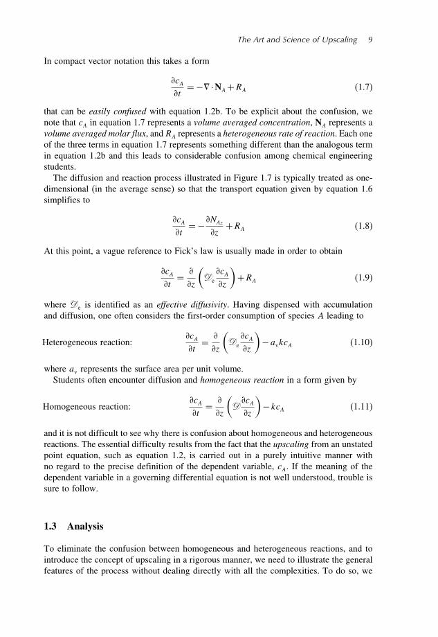
The Art and Science of Upscaling 9
In compact vector notation this takes a form
cAt
=− ·NA+RA (1.7)
that can be easily confused with equation 1.2b. To be explicit about the confusion, wenote that cA in equation 1.7 represents a volume averaged concentration, NA represents avolume averaged molar flux, and RA represents a heterogeneous rate of reaction. Each oneof the three terms in equation 1.7 represents something different than the analogous termin equation 1.2b and this leads to considerable confusion among chemical engineeringstudents.The diffusion and reaction process illustrated in Figure 1.7 is typically treated as one-
dimensional (in the average sense) so that the transport equation given by equation 1.6simplifies to
cAt
=−NAz
z+RA (1.8)
At this point, a vague reference to Fick’s law is usually made in order to obtain
cAt
=
z
(De
cAz
)+RA (1.9)
where De is identified as an effective diffusivity. Having dispensed with accumulationand diffusion, one often considers the first-order consumption of species A leading to
Heterogeneous reaction:cAt
=
z
(De
cAz
)−avkcA (1.10)
where av represents the surface area per unit volume.Students often encounter diffusion and homogeneous reaction in a form given by
Homogeneous reaction:cAt
=
z
(DcAz
)−kcA (1.11)
and it is not difficult to see why there is confusion about homogeneous and heterogeneousreactions. The essential difficulty results from the fact that the upscaling from an unstatedpoint equation, such as equation 1.2, is carried out in a purely intuitive manner withno regard to the precise definition of the dependent variable, cA. If the meaning of thedependent variable in a governing differential equation is not well understood, trouble issure to follow.
1.3 Analysis
To eliminate the confusion between homogeneous and heterogeneous reactions, and tointroduce the concept of upscaling in a rigorous manner, we need to illustrate the generalfeatures of the process without dealing directly with all the complexities. To do so, we

10 Chemical Engineering
b
b 2r0
2L
γ-phase
κ-phase
Figure 1.9 Bundle of capillary tubes as a model porous medium
consider a bundle of capillary tubes as a model of a porous medium. This model isillustrated in Figure 1.9 where we have shown a bundle of capillary tubes of length 2Land radius r0. The fluid in the capillary tubes is identified as the -phase and the solidas the -phase. The porosity of this model porous medium is given by
porosity= r20/b2 (1.12)
and we will use to represent the porosity.Our model of diffusion and heterogeneous reaction in one of the capillary tubes
illustrated in Figure 1.9 is given by the following boundary value problem:
cA
t=D
[1r
r
(rcA
r
)+ 2cA
z2
] in the -phase (1.13)
BC1 cA = cA z= 0 (1.14)
BC2 −D
cA
r= kcA r = r0 (1.15)
BC3 cA
z= 0 z= L (1.16)
IC unspecified (1.17)
Here we have assumed that the catalytic surface at r = r0 is quasi-steady even though thediffusion process in the pore may be transient (Carbonell and Whitaker, 1984; Whitaker,1986b). Equations 1.13–1.17 represent the physical situation in the pore domain and weneed equations that represent the physical situation in the porous medium domain. Thisrequires that we develop the area-averaged form of equation 1.13 and that we determine

The Art and Science of Upscaling 11
under what circumstances the concentration at r = r0 can be replaced by the area-averagedconcentration, cA . The area-averaged concentration is defined by
cA =1
r20
r=r0∫
r=0
2 rcA dr (1.18)
and in order to develop an area-averaged or upscaled diffusion equation, we form theintrinsic area average of equation 1.13 to obtain
1
r20
r=r0∫
r=0
(cA
t
)2 r dr = D
1
r20
r=r0∫
r=0
1r
r
(rcA
r
)2 r dr
+ 1
r20
r=r0∫
r=0
(2cA
z2
)2 r dr
(1.19)
The first and last terms in this result can be expressed as
1
r20
r=r0∫
r=0
(cA
t
)2 r dr =
t
1
r20
r=r0∫
r=0
cA2 r dr
= cA
t(1.20)
1
r20
r=r0∫
r=0
(2cA
z2
)2 r dr = 2
z2
1
r20
r=r0∫
r=0
cA2 r dr
= 2cA
z2(1.21)
so that equation 1.19 takes the form
cAt
=D
2
r20
r=r0∫
r=0
r
(rcA
r
)dr
+D
2cAz2
(1.22)
Evaluation of the integral leads to
cAt
=D
2cAz2
+ 2D
r0
cA
r
∣∣∣∣r=r0
(1.23)
and we can make use of the boundary condition given by equation 1.15 to incorporatethe heterogeneous rate of reaction into the area-averaged diffusion equation. This gives
cAt
=D
2cAz2
− 2kr0
cA
∣∣∣∣r=r0
(1.24)
Here we remark that the boundary condition is joined with the governing differentialequation, and that means that the heterogeneous reaction rate in equation 1.15 is nowbeginning to ‘look like’ a homogeneous reaction rate in equation 1.24. This process, inwhich a boundary condition is joined to a governing differential equation, is inherentin all studies of multiphase transport processes. The failure to identify explicitly this

12 Chemical Engineering
process often leads to confusion concerning the difference between homogeneous andheterogeneous chemical reactions.Equation 1.24 poses a problem in that it represents a single equation containing two
concentrations. If we cannot express the concentration at the wall of the capillary tube interms of the area-averaged concentration, the area-averaged transport equation will be oflittle use to us and we will be forced to return to equations 1.13–1.17 to solve the boundaryvalue problem by classical methods. In other words, the upscaling procedure would failwithout what is known as a method of closure. In order to complete the upscaling processin a simple manner, we need an estimate of the variation of the concentration acrossthe tube. We obtain this by using the flux boundary condition to construct the followingorder of magnitude estimate:
D
(cA∣∣r=0
− cA∣∣r=r0
r0
)=O
(k cA
∣∣r=r0
)(1.25)
which can be arranged in the form
cA∣∣r=0
− cA∣∣r=r0
cA∣∣r=r0
=O(kr0D
)(1.26)
When kr0/D 1 it should be clear that we can use the approximation
cA∣∣r=r0
= cA (1.27)
which represents the closure for this particular process. This allows us to express equa-tion 1.24 as
cAt
=D
2cAz2
− 2kr0
cAkr0D
1 (1.28)
Here we see that the heterogeneous reaction rate expression that appears in the fluxboundary condition given by equation 1.15 now appears as a homogeneous reaction rateexpression in the area-averaged transport equation. It should be clear that the ‘homoge-neous reaction rate coefficient’ contains the geometrical parameter, r0, and this is a clearindication that 2k/r0 is something other than a true homogeneous reaction rate coefficient.When the constraint, kr0/D 1, is not satisfied, the closure represented by equation 1.27becomes more complex and this condition has been explored by Paine et al. (1983).
1.3.1 Porous Catalysts
When dealing with porous catalysts, one generally does not work with the intrinsicaverage transport equation given by
cAt︸ ︷︷ ︸
accumulationper unit volume
of fluid
=D
2cAz2︸ ︷︷ ︸
diffusive fluxper unit volume
of fluid
− 2kr0
cA︸ ︷︷ ︸reaction rate
per unit volumeof fluid
(1.29)

The Art and Science of Upscaling 13
Here we have emphasized the intrinsic nature of our area-averaged transport equation,and this is especially clear with respect to the last term which represents the rate ofreaction per unit volume of the fluid phase. In the study of diffusion and reaction in realporous media (Whitaker, 1986a, 1987), it is traditional to work with the rate of reactionper unit volume of the porous medium. Since the ratio of the fluid volume to the volumeof the porous medium is the porosity, i.e.
= porosity=
volume
of the fluid
volume of theporous medium
(1.30)
the superficial averaged diffusion-reaction equation is expressed as
cAt︸ ︷︷ ︸
accumulation perunit volume ofporous media
= D
2cAz2︸ ︷︷ ︸
diffusive flux perunit volume ofporous media
− 2k
r0cA
︸ ︷︷ ︸rate of reactionper unit volumeof porous media
(1.31)
Here we see that the last term represents the rate of reaction per unit volume of theporous medium and this is the traditional interpretation in reactor design literature. Onecan show that 2/r0 represents the surface area per unit volume of the porous medium,and we denote this by av so that equation 1.31 takes the form
cAt
= D
2cAz2
−avkcA (1.32)
Sometimes the model illustrated in Figure 1.9 is extended to include tortuous pores suchas shown in the two-dimensional illustration in Figure 1.10. Under these circumstancesone often writes equation 1.32 in the form
cAt
= D
2cAz2
−avkcA (1.33)
γ-phase
κ-phase
Figure 1.10 Tortuous capillary tube as a model porous medium

14 Chemical Engineering
Here is a coefficient referred to as the tortuosity and the ratio, D/, is called theeffective diffusivity which is represented by Deff . This allows us to express equation 1.33in the traditional form given by
cAt
= Deff
2cAz2
−avkcA (1.34)
The step from equation 1.32 for a bundle of capillary tubes to equation 1.34 for a porousmedium is intuitive, and for undergraduate courses in reactor design one might acceptthis level of intuition. However, the development leading from equations 1.13 through1.17 to the upscaled result given by equation 1.32 is analytical and this level of analysisis necessary for an undergraduate course in reactor design. The more practical problemdeals with non-dilute solution diffusion and reaction in porous catalysts, and a rigorousanalysis of that case is given in the following sections.
1.4 Coupled, Non-linear Diffusion and Reaction
Problems of isothermal mass transfer and reaction are best represented in terms of thespecies continuity equation and the associated jump condition. We repeat these twoequations here as
cA
t+ · (cAvA
)= RA A= 12 N (1.35)
cAst
= (cAvA) ·n+RAs at the − interface A= 12 N (1.36)
A complete description of the mass transfer process requires a connection between thesurface concentration, cAs, and the bulk concentration, cA . One classic connection isbased on local mass equilibrium, and for a linear equilibrium relation this concept takesthe form
cAs = KAcA at the − interface A= 12 N (1.37a)
The condition of local mass equilibrium can exist even when adsorption and chemicalreaction are taking place (Whitaker, 1999, Problem 1-3). When local mass equilibriumis not valid, one must propose an interfacial flux constitutive equation. The classic linearform is given by (Langmuir, 1916, 1917)
(cAvA
) ·n = kA1cA −k−A1cAs at the − interface A= 12 N (1.37b)
where kA1 and k−A1 represent the adsorption and desorption rate coefficients for species A.In addition to equations 1.35 and 1.36, we need N momentum equations (Whitaker,
1986a) that are used to determine the N species velocities represented by vA ,A= 12 N . There are certain problems for which the N momentum equationsconsist of the total, or mass average, momentum equation
t
(v
)+ · (vv)= b + ·T (1.38)

The Art and Science of Upscaling 15
along with N −1 Stefan–Maxwell equations that take the form
0=−xA +E=N∑E=1E =A
xAxEvE −vA
DAE
A= 12 N −1 (1.39)
This form of the species momentum equation is acceptable when molecule–moleculecollisions are much more frequent than molecule–wall collisions; thus equation 1.39 isinappropriate when Knudsen diffusion must be taken into account. The species velocityin equation 1.39 can be decomposed into an average velocity and a diffusion velocityin more than one way (Taylor and Krishna, 1993; Slattery, 1999; Bird et al., 2002),and arguments are often given to justify a particular choice. In this work we prefera decomposition in terms of the mass average velocity because governing equations,such as the Navier–Stokes equations, are available to determine this velocity. The massaverage velocity in equation 1.38 is defined by
v =A=N∑A=1
AvA (1.40)
and the associated mass diffusion velocity is defined by the decomposition
vA = v +uA (1.41)
The mass diffusive flux has the attractive characteristic that the sum of the fluxes iszero, i.e.
A=N∑A=1
AuA = 0 (1.42)
As an alternative to equations 1.40–1.42, we can define a molar average velocity by
v∗ =A=N∑A=1
xAvA (1.43)
and the associated molar diffusion velocity is given by
vA = v∗ +u∗A (1.44)
In this case, the molar diffusive flux also has the attractive characteristic given by
A=N∑A=1
cAu∗A = 0 (1.45)
However, the use of the molar average velocity defined by equation 1.43 presents prob-lems when equation 1.38 must be used as one of the N momentum equations.If we make use of the mass average velocity and the mass diffusion velocity as
indicated by equations 1.40 and 1.41, the molar flux in equation 1.35 takes the form
cAvA︸ ︷︷ ︸total molar
flux
= cAv︸ ︷︷ ︸molar convective
flux
+ cAuA︸ ︷︷ ︸mixed-modediffusive flux
(1.46)
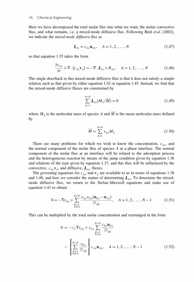
16 Chemical Engineering
Here we have decomposed the total molar flux into what we want, the molar convectiveflux, and what remains, i.e. a mixed-mode diffusive flux. Following Bird et al. (2002),we indicate the mixed-mode diffusive flux as
JA = cAuA A= 12 N (1.47)
so that equation 1.35 takes the form
cA
t+ · (cAv
)=− ·JA +RA A= 12 N (1.48)
The single drawback to this mixed-mode diffusive flux is that it does not satisfy a simplerelation such as that given by either equation 1.42 or equation 1.45. Instead, we find thatthe mixed-mode diffusive fluxes are constrained by
A=N∑A=1
JAMA/M= 0 (1.49)
where MA is the molecular mass of species A and M is the mean molecular mass definedby
M =A=N∑A=1
xAMA (1.50)
There are many problems for which we wish to know the concentration, cA , andthe normal component of the molar flux of species A at a phase interface. The normalcomponent of the molar flux at an interface will be related to the adsorption processand the heterogeneous reaction by means of the jump condition given by equation 1.36and relations of the type given by equation 1.37, and this flux will be influenced by theconvective, cAv , and diffusive, JA , fluxes.The governing equations for cA and v are available to us in terms of equations 1.38
and 1.48, and here we consider the matter of determining JA . To determine the mixed-mode diffusive flux, we return to the Stefan–Maxwell equations and make use ofequation 1.41 to obtain
0=−xA +E=N∑E=1E =A
xAxEuE −uA
DAE
A= 12 N −1 (1.51)
This can be multiplied by the total molar concentration and rearranged in the form
0 = −cxA +xA
E=N∑E=1E =A
cEuE
DAE
−
E=N∑E=1E =A
xE
DAE
cAuA A= 12 N −1 (1.52)

The Art and Science of Upscaling 17
which can then be expressed in terms of equation 1.47 to obtain
0 = −cxA +xA
E=N∑E=1E =A
JEDAE
−
E=N∑E=1E =A
xE
DAE
JA A= 12 N −1 (1.53)
Here we can use the classic definition of the mixture diffusivity
1DAm
=E=N∑E=1E =A
xE
DAE
(1.54)
in order to express equation 1.53 as
JA −xA
E=N∑E=1E =A
DAm
DAE
JE =−cDAmxA A= 12 N −1 (1.55)
When the mole fraction of species A is small compared to 1, we obtain the dilute solutionrepresentation for the diffusive flux
JA =−cDAmxA xA 1 (1.56)
and the transport equation for species A takes the form
cA
t+ · (cAv
)= · (cDAmxA)+RA xA 1 (1.57)
Given the condition xA 1, it is often plausible to impose the condition
xAc cxA (1.58)
and this leads to the following convective-diffusion equation that is ubiquitous in thereactor design literature:
cA
t+ · (cAv
)= · (DAmcA)+RA xA 1 (1.59)
When the mole fraction of species A is not small compared to 1, the diffusive flux in thistransport equation will not be correct. If the diffusive flux plays an important role in therate of heterogeneous reaction, equation 1.59 will not lead to a correct representation forthe rate of reaction.

18 Chemical Engineering
1.5 Diffusive Flux
We begin our analysis of the diffusive flux with equation 1.55 in the form
JA =−cDAmxA +xA
E=N∑E=1E =A
DAm
DAE
JE A= 12 N −1 (1.60)
and make use of equation 1.49 in an alternate form
A=N∑A=1
JA MA/MN= 0 (1.61)
in order to obtain N equations relating to the N diffusive fluxes. At this point we definea matrix R according to
R=
1 − xADAm
DAB
− xADAm
DAC
− · · · − xADAm
DAN
−xBDBm
DBA
+ 1 − xBDBm
DBC
− · · · − xBDBm
DBN
−xCDCm
DCA
− xCDCm
DCB
+ 1 − · · · − xCDCm
DCN
· · · · · − · · · − ·· · · · · − · · · − ·
MA
MN
+ MB
MN
+ MC
MN
+ · · · + 1
(1.62)and use equations 1.60 and 1.61 to express the N diffusive fluxes according to
R
JAJBJC· · ·· · ·JN
=−c
DAmxADBmxBDCmxC
· · ·DN−1mxN−1
0
(1.63)
We assume that the inverse of R exists in order to express the column matrix of diffusiveflux vectors in the form
JAJBJC· · ·· · ·JN
=−c R
−1
DAmxADBmxBDCmxC
· · ·DN−1mxN−1
0
(1.64)

The Art and Science of Upscaling 19
where the column matrix on the right-hand side of this result can be expressed as
DAmxADBmxBDCmxC
· · ·DN−1mxN−1
0
=
DAm 0 0 · · · 0 00 DBm 0 · · · 0 00 0 DCm · · · 0 0· · · · · · · ·0 0 0 · · · DN−1m 00 0 0 · · · 0 DNm
xAxBxC· · ·
xN−1
0
(1.65)
The diffusivity matrix is now defined by
D= R−1
DAm 0 0 · · · 0 00 DBm 0 · · · 0 00 0 DCm · · · 0 0· · · · · · · ·0 0 0 · · · DN−1m 00 0 0 · · · 0 DNm
(1.66)
so that equation 1.64 takes the form
JAJBJC· · ·· · ·JN
=−cD
xAxBxC· · ·
xN−1
0
(1.67)
This result can be expressed in a form analogous to that given by equation 1.60 leading to
JA =−c
E=N−1∑E=1
DAExE A= 12 N (1.68)
In the general case, the elements of the diffusivity matrix, DAE , will depend on the molefractions in a non-trivial manner. When this result is used in equation 1.48 we obtain thenon-linear, coupled governing differential equation for cA given by
cA
t+ ·
(cAv
)= ·
(c
E=N−1∑E=1
DAExE
)+RA A= 12 N (1.69)
We seek a solution to this equation subject to the jump condition given by equation 1.36and this requires knowledge of the concentration dependence of the homogeneous andheterogeneous reaction rates and information concerning the equilibrium adsorptionisotherm. In general, a solution of equation 1.69 for the system shown in Figure 1.7requires upscaling from the point scale to the pore scale and this can be done by themethod of volume averaging (Whitaker, 1999).

20 Chemical Engineering
1.6 Volume Averaging
To obtain the volume-averaged form of equation 1.69, we first associate an averagingvolume with every point in the − system illustrated in Figure 1.7. One such averagingvolume is illustrated in Figure 1.11, and it can be represented in terms of the volumes ofthe individual phases according to
V= V +V (1.70)
The radius of the averaging volume is r0 and the characteristic length scale associatedwith the -phase is indicated by as shown in Figure 1.11. In this figure we have alsoillustrated a length L that is associated with the distance over which significant changesin averaged quantities occur. Throughout this analysis we will assume that the lengthscales are disparate, i.e. the length scales are constrained by
L r0 (1.71)
Here the length scale, L, is a generic length scale (Whitaker, 1999, Sec. 1.3.2) determinedby the gradient of the average concentration, and all three quantities in equation 1.71are different to those listed in equation 1.1. We will use the averaging volume V todefine two averages: the superficial average and the intrinsic average. Each of theseaverages is routinely used in the description of multiphase transport processes, and it is
γ-phase
κ-phase
Averagingvolume, V
r0
γ
L
Figure 1.11 Averaging volume for a porous catalyst
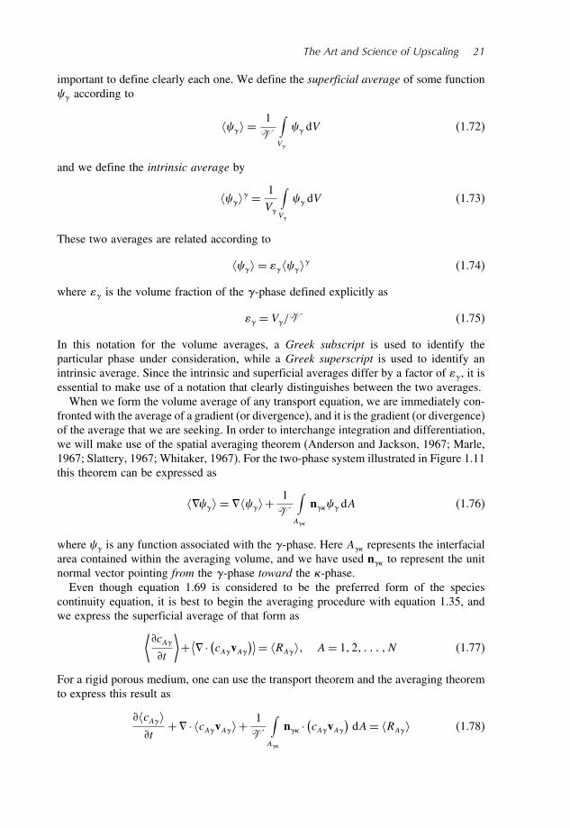
The Art and Science of Upscaling 21
important to define clearly each one. We define the superficial average of some function according to
=1V
∫
V
dV (1.72)
and we define the intrinsic average by
=1V
∫
V
dV (1.73)
These two averages are related according to
= (1.74)
where is the volume fraction of the -phase defined explicitly as
= V/V (1.75)
In this notation for the volume averages, a Greek subscript is used to identify theparticular phase under consideration, while a Greek superscript is used to identify anintrinsic average. Since the intrinsic and superficial averages differ by a factor of , it isessential to make use of a notation that clearly distinguishes between the two averages.When we form the volume average of any transport equation, we are immediately con-
fronted with the average of a gradient (or divergence), and it is the gradient (or divergence)of the average that we are seeking. In order to interchange integration and differentiation,we will make use of the spatial averaging theorem (Anderson and Jackson, 1967; Marle,1967; Slattery, 1967; Whitaker, 1967). For the two-phase system illustrated in Figure 1.11this theorem can be expressed as
= +1V
∫
A
n dA (1.76)
where is any function associated with the -phase. Here A represents the interfacialarea contained within the averaging volume, and we have used n to represent the unitnormal vector pointing from the -phase toward the -phase.Even though equation 1.69 is considered to be the preferred form of the species
continuity equation, it is best to begin the averaging procedure with equation 1.35, andwe express the superficial average of that form as
⟨cA
t
⟩+ ⟨ · (cAvA
)⟩= RA A= 12 N (1.77)
For a rigid porous medium, one can use the transport theorem and the averaging theoremto express this result as
cAt
+ · cAvA+1V
∫
A
n ·(cAvA
)dA= RA (1.78)

22 Chemical Engineering
where it is understood that this applies to all N species. Since we seek a transportequation for the intrinsic average concentration, we make use of equation 1.74 to expressequation 1.78 in the form
cAt
+ · cAvA+1V
∫
A
n ·(cAvA
)dA= RA (1.79)
At this point, it is convenient to make use of the jump condition given by equation 1.36in order to obtain
cAt
+ · cAvA = RA −1V
∫
A
cAst
dA+ 1V
∫
A
RAs dA (1.80)
We now define the intrinsic interfacial area average according to
=1A
∫
A
dA (1.81)
so that equation 1.80 takes the convenient form given by
cAt︸ ︷︷ ︸
accumulation
+ · cAvA︸ ︷︷ ︸transport
= RA︸ ︷︷ ︸homogeneous
reaction
−av
cAst︸ ︷︷ ︸
adsorption
+avRAs︸ ︷︷ ︸heterogeneous
reaction
(1.82)
One must keep in mind that this is a general result based on equations 1.35 and 1.36;however, only the first term in equation 1.82 is in a form that is ready for applications.
1.7 Chemical Reactions
In general, the homogeneous reaction will be of no consequence in a porous catalyst andwe need only direct our attention to the heterogeneous reaction represented by the lastterm in equation 1.82. The chemical kinetic constitutive equation for the heterogeneousrate of reaction can be expressed as
RAs = RAs cAs cBs cN s (1.83)
and here we see the need to relate the surface concentrations, cAs cBs cN s, to thebulk concentrations, cA cB cN , and subsequently to the local volume-averagedconcentrations, cA cB cN . In order for heterogeneous reaction to occur,adsorption at the catalytic surface must also occur. However, there are many transientprocesses of mass transfer with heterogeneous reaction for which the catalytic surfacecan be treated as quasi-steady (Carbonell and Whitaker, 1984; Whitaker, 1986b). Whenhomogeneous reactions can be ignored and the catalytic surface can be treated as quasi-steady, the local volume-averaged transport equation simplifies to
cAt︸ ︷︷ ︸
accumulation
+ · cAvA︸ ︷︷ ︸transport
= avRAs︸ ︷︷ ︸heterogeneous
reaction
(1.84)
and this result provides the basis for several special forms.

The Art and Science of Upscaling 23
1.8 Convective and Diffusive Transport
Before examining the heterogeneous reaction rate in equation 1.84, we consider thetransport term, cAvA. We begin with the mixed-mode decomposition given by equa-tion 1.46 in order to obtain
cAvA︸ ︷︷ ︸total molar
flux
= cAv︸ ︷︷ ︸molar convective
flux
+cAuA︸ ︷︷ ︸mixed-modediffusive flux
(1.85)
Here the convective flux is given in terms of the average of a product, and we want toexpress this flux in terms of the product of averages. As in the case of turbulent transport,this suggests the use of decompositions given by
cA = cA + cA v = v + v (1.86)
At this point one can follow a detailed analysis (Whitaker, 1999, Chapter 3) of theconvective transport to arrive at
cAvA︸ ︷︷ ︸total flux
= cAv︸ ︷︷ ︸average convective
flux
+cA v︸ ︷︷ ︸dispersive
flux
+ JA︸ ︷︷ ︸mixed-modediffusive flux
(1.87)
Here we have used the intrinsic average concentration since this is most closely relatedto the concentration in the fluid phase, and we have used the superficial average velocitysince this is the quantity that normally appears in Darcy’s law (Whitaker, 1999) or theForchheimer equation (Whitaker, 1996). Use of equation 1.87 in equation 1.84 leads to
cAt
+ · (cAv)=− · JA︸ ︷︷ ︸
diffusivetransport
− · cA v︸ ︷︷ ︸dispersivetransport
+avRAs︸ ︷︷ ︸heterogeneous
reaction
(1.88)
If we treat the catalytic surface as quasi-steady and make use of a simple first-order,irreversible representation for the heterogeneous reaction, we can show that RAs is givenby (Whitaker, 1999, Sec. 1.1)
RAs =−kAscAs =−(
kAskA1kAs+k−A1
)cA at the − interface (1.89)
when species A is consumed at the catalytic surface. Here we have used kAs to representthe intrinsic surface reaction rate coefficient, while kA1 and k−A1 are the adsorption anddesorption rate coefficients that appear in equation 1.37b. Other more complex reactionmechanisms can be proposed; however, if a linear interfacial flux constitutive equation isvalid, the heterogeneous reaction rates can be expressed in terms of the bulk concentrationas indicated by equation 1.89. Under these circumstances the functional dependenceindicated in equation 1.83 can be simplified to
RAs = RAs
(cA cB cN
) at the − interface (1.90)

24 Chemical Engineering
Given the type of constraints developed elsewhere (Wood and Whitaker, 1998, 2000),the interfacial area average of the heterogeneous rate of reaction can be expressed as
RAs = RAs(cA cB cN
) at the − interface (1.91)
Sometimes confusion exists concerning the idea of an area-averaged bulk concentration,and to clarify this idea we consider the averaging volume illustrated in Figure 1.12. In thisfigure we have shown an averaging volume with the centroid located (arbitrarily) in the-phase. In this case, the area average of the bulk concentration is given explicitly by
cA∣∣x= 1
Ax
∫
Ax
cA∣∣x+y
dA (1.92)
where x locates the centroid of the averaging volume and y locates points on the –interface. We have used Ax to represent the area of the – interface containedwithin the averaging volume.To complete our analysis of equation 1.91, we need to know how the area-averaged
concentration, cA, is related to the volume-averaged concentration, cA . Whenconvective transport is important, relating cA to cA requires some analysis;however, when diffusive transport dominates in a porous catalyst the area-averagedconcentration is essentially equal to the volume-averaged concentration. This occursbecause the pore Thiele modulus is generally small compared to one and the typeof analysis indicated by equations 1.24–1.28 is applicable. Under these circumstances,equation 1.91 can be expressed as
RAs = RAs(cA cB cN
) at the − interface (1.93)
y
x
γ-phase
V
κ-phase
Figure 1.12 Position vectors associated with the area average over the – interface
The Art and Science of Upscaling 25
and equation 1.88 takes the form
cAt
+ · (cAv) = − · JA− · cA v
+avRAs(cA cB cN
)(1.94)
In porous catalysts one often neglects convective transport indicated by
cA v cAv JA (1.95)
and this leads to a transport equation that takes the form
cAt
= − · JA+avRAs
(cA cB cN) A= 12 N (1.96)
This result forms the basis for the classic problem of diffusion and reaction in a porouscatalyst such as we have illustrated in Figure 1.5. It is extremely important to recognizethat the mathematical consequence of equations 1.95 and 1.96 is that the mass averagevelocity has been set equal to zero; thus our substitute for equation 1.38 is given bythe assumption
v = 0 (1.97)
This assumption requires that we discard the momentum equation given by equation 1.38and proceed to develop a solution to our mass transfer process in terms of the N −1momentum equations represented by equation 1.39. The inequalities contained in equa-tion 1.95 are quite appealing when one is dealing with a diffusion process; however,equation 1.97 is not satisfied by the Stefan diffusion tube process (Whitaker, 1991), noris it satisfied by the Graham’s law counter-diffusion process (Jackson, 1977). It shouldbe clear that the constraints associated with the equalities given by equation 1.95 needto be developed. When convective transport is retained, some results are available fromQuintard and Whitaker (2005); however, a detailed analysis of the coupled, non-linearprocess with convective transport remains to be done. At this point we leave those prob-lems for a subsequent study and explore the diffusion and reaction process described byequation 1.96.
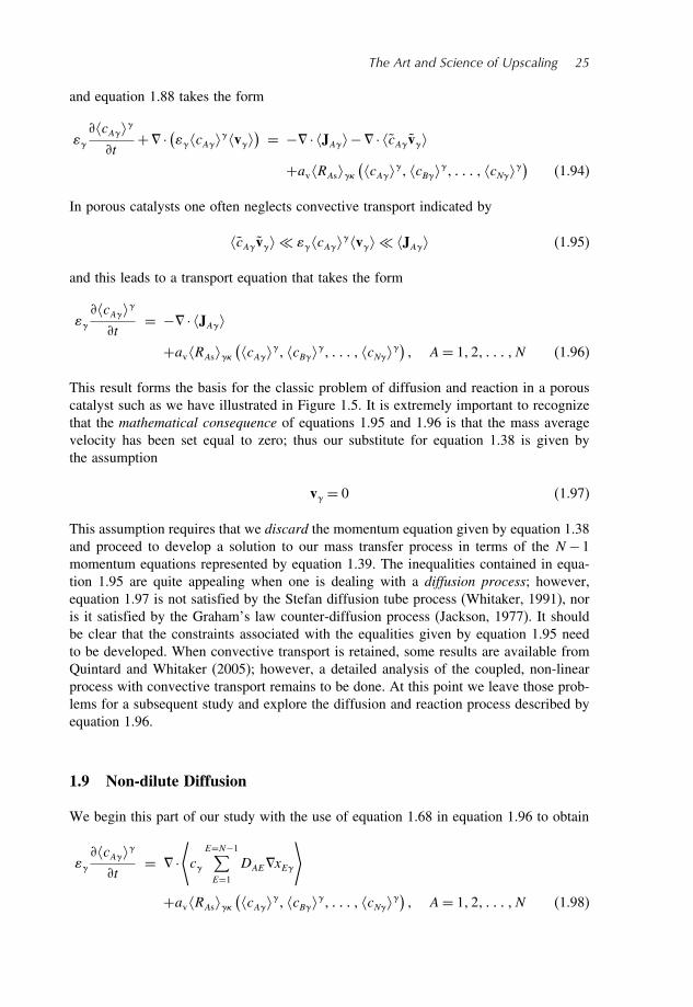
1.9 Non-dilute Diffusion
We begin this part of our study with the use of equation 1.68 in equation 1.96 to obtain
cAt
= ·⟨c
E=N−1∑E=1
DAExE
⟩
+avRAs(cA cB cN
) A= 12 N (1.98)

26 Chemical Engineering
where the diffusive flux is non-linear because DAE depends on the N −1 mole fractions.This transport equation must be solved subject to the auxiliary conditions given by
c =A=N∑A=1
cA 1=A=N∑A=1
xA (1.99)
and this suggests that numerical methods must be used. However, the diffusive flux mustbe arranged in terms of volume-averaged quantities before equation 1.98 can be solved,and any reasonable simplifications that can be made should be imposed on the analysis.
1.9.1 Constant Total Molar Concentration
Some non-dilute solutions can be treated as having a constant total molar concentrationand this simplification allows us to express equation 1.98 as
cAt
= ·⟨E=N−1∑E=1
DAEcE
⟩
+avRAs(cA cB cN
) A= 12 N (1.100)
The restriction associated with this simplification is given by
xAc cxA A= 12 N (1.101)
and it is important to understand that the mathematical consequence of this restriction isgiven by the assumption
c = c = constant (1.102)
Imposition of this condition means that there are only N − 1 independent transportequations of the form given by equation 1.100, and we shall impose this conditionthroughout the remainder of this study. The constraints associated with equation 1.102need to be developed and the more general case represented by equations 1.98 and 1.99should be explored.At this point we decompose the elements of the diffusion matrix according to
DAE = DAE + DAE (1.103)
and if we can neglect DAE relative to DAE , the transport equation given by equa-tion 1.100 simplifies to
cAt
= ·E=N−1∑E=1
DAEcE
+avRAs(cA cB cN−1
) A= 12 N −1
(1.104)We can represent this simplification as
DAE DAE (1.105)
and when it is not satisfactory it may be possible to develop a correction based on theretention of the spatial deviation, DAE . However, it is not clear how this type of analysiswould evolve and further study of this aspect of the diffusion process is in order.

The Art and Science of Upscaling 27
1.9.2 Volume Average of the Diffusive Flux
The volume-averaging theorem can be used with the average of the gradient in equa-tion 1.104 in order to obtain
cE = cE+1V
∫
A
ncE dA (1.106)
and one can follow an established analysis (Whitaker, 1999, Chapter 1) in order to expressthis result as
cE = cE +1V
∫
A
ncE dA (1.107)
Use of this result in equation 1.104 provides
cAt
= ·
E=N−1∑E=1
DAE
cE +
1V
∫
A
ncE dA
︸ ︷︷ ︸filter
+avRAs (1.108)
where the area integral of ncE has been identified as a filter. Not all the informationavailable at the length scale associated with cE will pass through this filter to influencethe transport equation for cA , and the existence of filters of this type is a recurringtheme in the method of volume averaging (Whitaker, 1999).
1.10 Closure
In order to obtain a closed form of equation 1.108, we need a representation for the spatialdeviation concentration, cA , and this requires the development of the closure problem.When convective transport is negligible and homogeneous reactions are ignored as beinga trivial part of the analysis, equation 1.48 takes the form
cA
t=− ·JA A= 12 N −1 (1.109)
Here one must remember that the total molar concentration is a specified constant; thusthere are only N−1 independent species continuity equations. Use of equation 1.68 alongwith the restriction given by equation 1.101 allows us to express this result as
cA
t= ·
E=N−1∑E=1
DAEcE A= 12 N −1 (1.110)
and on the basis of equations 1.103 and 1.105 this takes the form
cA
t= ·
E=N−1∑E=1
DAEcE A= 12 N −1 (1.111)

28 Chemical Engineering
If we ignore variations in and subtract equation 1.108 from equation 1.111, we canarrange the result as
cA
t= ·
[E=N−1∑E=1
DAEcE]
− ·E=N−1∑
E=1
DAE
1V
∫
A
ncE dA
− av
RAs (1.112)
where it is understood that this result applies to all N − 1 species. Equation 1.112represents the governing differential equation for the spatial deviation concentration, andin order to keep the analysis relatively simple we consider only the first-order, irreversiblereaction described by equation 1.89 and expressed here in the form
RAs =−kAcA at the − interface (1.113)
One must remember that this is a severe restriction in terms of realistic systems andmore general forms for the heterogeneous rate of reaction need to be examined. Use ofequation 1.113 in equation 1.112 leads to the following form:
cA
t= ·
[E=N−1∑E=1
DAEcE]
− ·E=N−1∑
E=1
DAE
1V
∫
A
ncE dA
+ avkA
cA (1.114)
Here we have made use of the simplification
cA = cA (1.115)
and the justification is given elsewhere (Whitaker, 1999, Sec. 1.3.3). In order to completethe problem statement for cE , we need a boundary condition for cE at the – interface.To develop this boundary condition, we again make use of the quasi-steady form ofequation 1.36 to obtain
JA ·n =−RAs at the − interface (1.116)
where we have imposed the restriction given by
v ·n uA ·n at the − interface (1.117)
This is certainly consistent with the inequalities given by equation 1.95; however, theneglect of v ·n relative to uA ·n is generally based on the dilute solution conditionand the validity of equation 1.117 is another matter that needs to be carefully consideredin a future study. On the basis of equations 1.68, 1.101, 1.103, and 1.105 along withequation 1.113, the jump condition takes the form
−E=N−1∑E=1
n · DAEcE = kAcA at the − interface (1.118)

The Art and Science of Upscaling 29
In order to express this boundary condition in terms of the spatial deviation concentration,we make use of the decomposition given by the first part of equation 1.86 to obtain
−E=N−1∑E=1
n · DAEcE −kAcA =E=N−1∑E=1
n · DAEcE
+kAcA at the − interface (1.119)
With this result we can construct the following boundary value problem for cA:
cA
t︸︷︷︸accumulation
= ·[E=N−1∑E=1
DAEcE]
︸ ︷︷ ︸diffusion
− ·E=N−1∑
E=1
DAE
1V
∫
A
ncE dA
︸ ︷︷ ︸non-local diffusion
+ avkA
cA︸ ︷︷ ︸
reactionsource
(1.120)
BC1 −E=N−1∑E=1
n · DAEcE︸ ︷︷ ︸
diffusive flux
− kAcA︸ ︷︷ ︸heterogeneous
reaction
=E=N−1∑E=1
n · DAEcE︸ ︷︷ ︸
diffusive source
+kAcA︸ ︷︷ ︸reactionsource
at the − interface
(1.121)
BC2 cA = Fr t at Ae (1.122)
IC cA = Fr at t = 0 (1.123)
In addition to the flux boundary condition given by equation 1.121, we have added anunknown condition at the macroscopic boundary of the -phase, Ae, and an unknowninitial condition. Neither of these is important when the separation of length scalesindicated by equation 1.71 is valid. Under these circumstances, the boundary conditionimposed at Ae influences the cA field only over a negligibly small region, and theinitial condition given by equation 1.123 can be discarded because the closure problemis quasi-steady. Under these circumstances, the closure problem can be solved in somerepresentative, local region (Quintard and Whitaker, 1994a–e).In the governing differential equation for cA , we have identified the accumulation term,
the diffusion term, the so-called non-local diffusion term, and the non-homogeneous termreferred to as the reaction source. In the boundary condition imposed at the – interface,we have identified the diffusive flux, the reaction term, and two non-homogeneous termsthat are referred to as the diffusion source and the reaction source. If the source termsin equations 1.120 and 1.121 were zero, the cA-field would be generated only by thenon-homogeneous terms that might appear in the boundary condition imposed at Ae
or in the initial condition given by equation 1.123. One can easily develop argumentsindicating that the closure problem for cA is quasi-steady, thus the initial condition is

30 Chemical Engineering
of no importance (Whitaker, 1999, Chapter 1). In addition, one can develop argumentsindicating that the boundary condition imposed at Ae will influence the cA field overa negligibly small portion of the field of interest. Because of this, any useful solutionto the closure problem must be developed for some representative region which is mostoften conveniently described in terms of a unit cell in a spatially periodic system. Theseideas lead to a closure problem of the form
0= ·[E=N−1∑E=1
DAEcE]
︸ ︷︷ ︸diffusion
− ·E=N−1∑
E=1
DAEV
∫
A
ncE dA
︸ ︷︷ ︸non-local diffusion
+ avkA
cA︸ ︷︷ ︸
reactionsource
(1.124)
BC1 −E=N−1∑E=1
n · DAEcE︸ ︷︷ ︸
diffusive flux
− kAcA︸ ︷︷ ︸heterogeneous
reaction
=E=N−1∑E=1
n · DAEcE︸ ︷︷ ︸
diffusive source
+kAcA︸ ︷︷ ︸reactionsource
at the − interface
(1.125)
BC2 cAr+i= cAr i= 123 (1.126)
Here we have used i to represent the three base vectors needed to characterize a spatiallyperiodic system. The use of a spatially periodic system does not limit this analysisto simple systems since a periodic system can be arbitrarily complex (Quintard andWhitaker, 1994a–e). However, the periodicity condition imposed by equation 1.126 canonly be strictly justified when DAE , cA , and cA are constants and this doesnot occur for the types of systems under consideration. This matter has been examinedelsewhere (Whitaker, 1986b) and the analysis suggests that the traditional separation oflength scales allows one to treat DAE , cA , and cA as constants within theframework of the closure problem.It is not obvious, but other studies (Ryan et al., 1981) have shown that the reaction
source in equations 1.124 and 1.125makes a negligible contribution to cA . In addition, onecan demonstrate (Whitaker, 1999) that the heterogeneous reaction, kAcA , can be neglectedfor all practical problems of diffusion and reaction in porous catalysts. Furthermore, thenon-local diffusion term is negligible for traditional systems, and under these circumstancesthe boundary value problem for the spatial deviation concentration takes the form
0= ·[E=N−1∑E=1
DAEcE]
(1.127)
BC1 −E=N−1∑E=1
n · DAEcE =E=N−1∑E=1
n · DAEcE at A (1.128)
BC2 cAr+i= cAr i= 123 (1.129)
Here one must remember that the subscript A represents species A, B, C, , N −1.

The Art and Science of Upscaling 31
In this boundary value problem, there is only a single non-homogeneous term rep-resented by cE in the boundary condition imposed at the – interface. If thissource term were zero, the solution to this boundary value problem would be given bycA = constant. Any constant associated with cA will not pass through the filter in equa-tion 1.108, and this suggests that a solution can be expressed in terms of the gradients ofthe volume-averaged concentration. Since the system is linear in the N −1 independentgradients of the average concentration, we are led to a solution of the form
cE = bEA ·cA +bEB ·cB +bEC ·cC +· · ·+bEN−1 ·cN−1 (1.130)
Here the vectors, bEA, bEB, etc., are referred to as the closure variables or the mappingvariables since they map the gradients of the volume-averaged concentrations onto thespatial deviation concentrations. In this representation for cA , we can ignore the spatialvariations of cA , cB , etc. within the framework of a local closure problem,and we can use equation 1.130 in equation 1.127 to obtain
0=
[E=N−1∑E=1
DAED=N−1∑D=1
bED ·cD]
(1.131)
BC1 −E=N−1∑E=1
n · DAED=N−1∑D=1
bED ·cD
=E=N−1∑E=1
n · DAEcE at A (1.132)
BC2 bAEr+i= bAEr i= 123 A= 12 N −1(1.133)
The derivation of equations 1.131 and 1.132 requires the use of simplifications of theform
(bEA ·cA
)= bEA ·cA (1.134)
which result from the inequality
bEA ·cA bEA ·cA (1.135)
The basis for this inequality is the separation of length scales indicated by equation 1.71,and a detailed discussion is available elsewhere (Whitaker, 1999). One should keep inmind that the boundary value problem given by equations 1.131–1.133 applies to allN − 1 species and that the N − 1 concentration gradients are independent. This lattercondition allows us to obtain
0= ·[E=N−1∑E=1
DAEbED
] D = 12 N −1 (1.136)
BC1 −E=N−1∑E=1
n · DAEbED = nDAD
D = 12 N −1 at A (1.137)
Periodicity bADr+i= bADr i= 123 D = 12 N −1(1.138)

32 Chemical Engineering
At this point it is convenient to expand the closure problem for species A in order toobtain
First problem for species A
0= ·DAA
[bAA+ DAA−1 DABbBA
+ DAA−1 DACbCA+· · ·+ DAA−1 DAN−1bN−1A
]
(1.139a)
−n ·bAA−n · DAA−1 DABbBA
BC −n · DAA−1 DACbCA−· · · (1.139b)
−n · DAA−1 DAN−1bN−1A = n at A
Periodicity bDAr+i= bDAr i= 123 D = 12 N −1(1.139c)
Second problem for species A
0= ·DAB
[DAB−1 DAAbAB+bBB
+ DAB−1 DACbCB+· · ·+ DAB−1 DAN−1bN−1B
]
(1.140a)
−n ·bAA−n · DAA−1 DABbBA
BC −n · DAA−1 DACbCA−· · · (1.140b)
−n · DAA−1 DAN−1bN−1A = n at A
Periodicity bDBr+i= bDBr i= 123 D = 12 N −1(1.140c)
Third problem for species A
etc (1.141)
N −1 problem for species A
etc (1.142)
Here it is convenient to define a new set of closure variables or mapping variablesaccording to
dAA = bAA+ DAA−1 DABbBA+ DAA−1 DACbCA
+· · ·+ DAA−1 DAN−1bN−1A (1.143a)
dAB = DAB−1 DAAbAB+bBB+ DAB−1 DACbCB
+· · ·+ DAB−1 DAN−1bN−1B (1.143b)

The Art and Science of Upscaling 33
dAC = DAC−1 DAAbAC + DAC−1 DABbBC +bCC
+· · ·+ DAC−1 DAN−1bN−1C (1.143c)
etc (1.143d)
With these definitions, the closure problems take the following simplified forms:
First problem for species A
0= 2dAA (1.144a)
BC −n ·dAA = n at A (1.144b)
Periodicity dAAr+i= dAAr i= 123(1.144c)
Second problem for species A
0= 2dAB (1.145a)
BC −n ·dAB = n at A (1.145b)
Periodicity dABr+i= dABr i= 123(1.145c)
Third problem for species A
etc (1.146)
N–1 problem for species A
etc (1.147)
To obtain these simplified forms, one must make repeated use of inequalities of theform given by equation 1.135. Each one of these closure problems is identical to thatobtained by Ryan et al. (1981) and solutions have been developed by several workers(Chang, 1982, 1983; Ochoa-Tapia et al., 1994; Quintard, 1993; Quintard and Whitaker,1993a,b; Ryan et al., 1981). In each case, the closure problem determines the closurevariable to within an arbitrary constant, and this constant can be specified by imposing thecondition
cD = 0 or dGD = 0G= 12 N −1D = 12 N −1
(1.148)
However, any constant associated with a closure variable will not pass through the filterin equation 1.108; thus this constraint on the average is not necessary.
34 Chemical Engineering
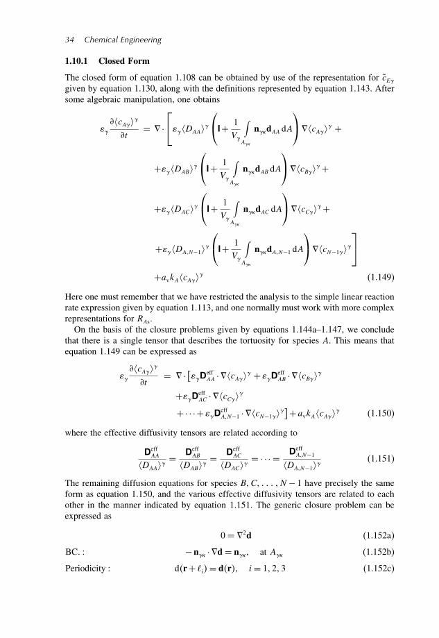
1.10.1 Closed Form
The closed form of equation 1.108 can be obtained by use of the representation for cEgiven by equation 1.130, along with the definitions represented by equation 1.143. Aftersome algebraic manipulation, one obtains
cAt
= ·DAA
I+ 1
V
∫
A
ndAA dA
cA +
+DABI+ 1
V
∫
A
ndAB dA
cB +
+DACI+ 1
V
∫
A
ndAC dA
cC +
+DAN−1I+ 1
V
∫
A
ndAN−1 dA
cN−1
+avkAcA (1.149)
Here one must remember that we have restricted the analysis to the simple linear reactionrate expression given by equation 1.113, and one normally must work with more complexrepresentations for RAs.On the basis of the closure problems given by equations 1.144a–1.147, we conclude
that there is a single tensor that describes the tortuosity for species A. This means thatequation 1.149 can be expressed as
cAt
= · [DeffAA ·cA +D
effAB ·cB
+DeffAC ·cC
+· · ·+DeffAN−1 ·cN−1
]+avkAcA (1.150)
where the effective diffusivity tensors are related according to
DeffAA
DAA= Deff
AB
DAB= Deff
AC
DAC= · · · = Deff
AN−1
DAN−1(1.151)
The remaining diffusion equations for species BC N −1 have precisely the sameform as equation 1.150, and the various effective diffusivity tensors are related to eachother in the manner indicated by equation 1.151. The generic closure problem can beexpressed as
0= 2d (1.152a)
BC −n ·d= n at A (1.152b)
Periodicity dr+i= dr i= 123 (1.152c)

The Art and Science of Upscaling 35
and solution of this boundary value problem is relatively straightforward. The existenceof a single generic closure problem that allows for the determination of all the effectivediffusivity tensors represents the main finding of this work. On the basis of this singleclosure problem, the tortuosity tensor is defined according to
= I+ 1V
∫
A
nddA (1.153)
and we can express equation 1.151 in the form
DeffAA = DAA Deff
AB = DAB DeffAN−1 = DAN−1 (1.154)
Substitution of these results into equation 1.150 allows us to represent the local volume-averaged diffusion-reaction equations as
cAt
= ·[E=N−1∑E=1
DAE ·cE]
+avkAcA A= 12 N −1 (1.155)
It is important to remember that this analysis has been simplified on the basis of equa-tion 1.101 which is equivalent to treating c as a constant as indicated in equation 1.102.For a porous medium that is isotropic in the volume-averaged sense, the tortuosity tensortakes the classical form
= I−1 (1.156)
where I is the unit tensor and is the tortuosity. For isotropic porous media, we canexpress equation 1.155 as
cAt
= ·[E=N−1∑E=1
(/
) DAEcE]
+avkAcA A= 12 N −1 (1.157)
Often and can be treated as constants; however, the diffusion coefficients in thistransport equation will be functions of the local volume-averaged mole fractions and weare faced with a coupled, non-linear diffusion and reaction problem.
1.11 Conclusions
In this chapter we have first shown how an intuitive upscaling procedure can lead toconfusion regarding homogeneous and heterogeneous reactions, and in a more formaldevelopment we have shown how the coupled, non-linear diffusion problem can be

36 Chemical Engineering
analyzed to produce volume-averaged transport equations containing effective diffusivitytensors. The original diffusion-reaction problem is described by
cA
t= ·
E=N−1∑E=1
DAEcE A= 12 N −1 (1.158a)
BC −E=N−1∑E=1
n ·DAEcE = kAcA at the − interface (1.158b)
c = c = constant (1.158c)
where the DAE are functions of the mole fractions. For a porous medium that is isotropicin the volume-averaged sense, the upscaled version of the diffusion-reaction problemtakes the form
cAt
= ·[E=N−1∑E=1
(/
) DAEcE]
+avkAcA A= 12 N −1 (1.159)
Here we have used the approximation that DAE can be replaced by DAE and thatvariations of DAE can be ignored within the averaging volume. The fact that onlya single tortuosity needs to be determined by equations 1.152 and 1.153 representsthe key contribution of this study. It is important to remember that this developmentis constrained by the linear chemical kinetic constitutive equation given by equa-tion 1.113. The process of diffusion in porous catalysts is normally associated withslow reactions and equation 1.93 is satisfactory; however, the first-order, irreversiblereaction represented by equation 1.113 is the exception rather than the rule, and thisaspect of the analysis requires further investigation. The influence of a non-zero massaverage velocity needs to be considered in future studies so that the constraint givenby equation 1.97 can be removed. An analysis of that case is reserved for a futurestudy which will also include a careful examination of the simplification indicated byequation 1.117.
Nomenclature
Ae area of entrances and exits of the -phase contained in the macroscopicregion, m2
A area of the − interface contained within the averaging volume, m2
av A/V , area per unit volume, 1/mb body force vector, m/s2
cA bulk concentration of species A in the -phase, moles/m3
cA superficial average bulk concentration of species A in the -phase, moles/m3
cA intrinsic average bulk concentration of species A in the -phase, moles/m3
cA intrinsic area average bulk concentration of species A at the − interface,moles/m3
cA cA −cA , spatial deviation concentration of species A, moles/m3

The Art and Science of Upscaling 37
cA=N∑A=1
cA , total molar concentration, moles/m3
cAs surface concentration of species A associated with the − interface,moles/m2
DAB binary diffusion coefficient for species A and B, m2/s
DAm D−1Am = E=N∑
E=1E =A
xE/DAE , mixture diffusivity, m2/s
D diffusivity matrix, m2/sDAE element of the diffusivity matrix, m2/sDAE intrinsic average element of the diffusivity matrix, m2/sDAE DAE −DAE , spatial deviation of an element of the diffusivity matrix, m2/sJA cAuA , mixed-mode diffusive flux, mole/m2sKA adsorption equilibrium coefficient for species A, mkA1 adsorption rate coefficient for species A, m/sk−A1 desorption rate coefficient for species A, 1/skAs surface reaction rate coefficient, 1/s small length scale associated with the -phase, mr0 radius of the averaging volume, mL large length scale associated with the porous medium, mMA molecular mass of species A, kg/kg mole
MA=N∑A=1
xAMA, mean molecular mass, kg/kg mole
n unit normal vector directed from the -phase to the -phaser position vector, mRA rate of homogeneous reaction in the - phase, moles/m3sRAs rate of heterogeneous reaction associated with the − interface,
moles/m2sRAs area average heterogeneous reaction rate for species A, moles/m2st time, sT stress tensor for the -phase, N/m2
uA vA −v , mass diffusion velocity, m/su∗A vA −v∗ , molar diffusion velocity, m/s
vA velocity of species A in the -phase, m/s
vA=N∑A=1
AvA , mass average velocity in the -phase, m/s
v∗A=N∑A=1
xAvA , molar average velocity in the -phase, m/s
v intrinsic mass average velocity in the -phase, m/sv superficial mass average velocity in the -phase, m/sv v −v , spatial deviation velocity, m/sV averaging volume, m3
V volume of the -phase contained within the averaging volume, m3
V volume of the -phase contained within the averaging volume, m3
xA cA/c , mole fraction of species A in the -phasex position vector locating the center of the averaging volume, my position vector locating points on the − interface relative to the center of
the averaging volume, m

38 Chemical Engineering
Greek letters
volume fraction of the -phase (porosity)A mass density of species A in the -phase, kg/m3
mass density for the -phase, kg/m3
A A/ , mass fraction of species A in the -phase
References
Anderson T.B. and Jackson R. 1967. A fluid mechanical description of fluidized beds, Ind. Engng.Chem. Fundam., 6, 527–538.
Bird R.B., Steward W.E. and Lightfoot E.N. 2002. Transport Phenomena, 2nd edition. John Wiley& Sons, New York.
Birkhoff G. 1960. Hydrodynamics: A Study in Logic, Fact, and Similitude. Princeton UniversityPress, Princeton, New Jersey.
Butt J.B. 1980. Reaction Kinetics and Reactor Design. Prentice-Hall, Englewood Cliffs,New Jersey.
Carberry J.J. 1976. Chemical and Catalytic Reaction Engineering. McGraw-Hill, New York.Carbonell R.G. and Whitaker S. 1984. Adsorption and reaction at a catalytic surface: The quasi-
steady condition, Chem. Eng. Sci., 39, 1319–1321.Chang H-C. 1982. Multiscale analysis of effective transport in periodic heterogeneous media,
Chem. Eng. Commun., 15, 83–91.Chang H-C. 1983. Effective diffusion and conduction in two-phase media: A unified approach,
AIChE J., 29, 846–853.Cushman J.H. 1990. Dynamics of Fluids in Hierarchical Porous Media. Academic Press, London.Fogler H.S. 1992. Elements of Chemical Reaction Engineering. Prentice Hall, Englewood Cliffs,
New Jersey.Froment G.F. and Bischoff K.B. 1979. Chemical Reactor Analysis and Design. John Wiley &
Sons, New York.Jackson R. 1977. Transport in Porous Catalysts. Elsevier, New York.Langmuir I. 1916. The constitution and fundamental properties of solids and liquids I: Solids, J.
Am. Chem. Soc., 38, 2221–2295.Langmuir I. 1917. The constitution and fundamental properties of solids and liquids II: Liquids, J.
Am. Chem. Soc., 39, 1848–1906.Levenspiel O. 1999. Chemical Reaction Engineering, 3rd edition. John Wiley & Sons, New York.Marle C.M. 1967. Écoulements monophasique en milieu poreux, Rev. Inst. Français du Pétrole,
22(10), 1471–1509.Ochoa-Tapia J.A., del Río J.A. and Whitaker S. 1993. Bulk and surface diffusion in porous media:
An application of the surface averaging theorem, Chem. Eng. Sci., 48, 2061–2082.Ochoa-Tapia J.A., Stroeve P. and Whitaker S. 1994. Diffusive transport in two-phase media:
Spatially periodic models and Maxwell’s theory for isotropic and anisotropic systems, Chem.Eng. Sci., 49, 709–726.
Paine M.A., Carbonell R.G. and Whitaker S. 1983. Dispersion in pulsed systems I: Heterogeneousreaction and reversible adsorption in capillary tubes, Chem. Eng. Sci., 38, 1781–1793.
Quintard M. 1993. Diffusion in isotropic and anisotropic porous systems: Three-dimensional cal-culations, Transport Porous Med., 11, 187–199.
Quintard M. and Whitaker S. 1993a. Transport in ordered and disordered porous media: Volumeaveraged equations, closure problems, and comparison with experiment, Chem. Eng. Sci., 48,2537–2564.

The Art and Science of Upscaling 39
Quintard M. andWhitaker S. 1993b. One- and two-equation models for transient diffusion processesin two-phase systems. In, Advances in Heat Transfer, Harnett J.P., Irvine T.F. Jr and Cho Y.I.(Eds.), Vol. 23. Academic Press, New York, pp. 369–465.
Quintard M. and Whitaker S. 1994a. Transport in ordered and disordered porous media I: Thecellular average and the use of weighting functions, Transport Porous Med., 14, 163–177.
Quintard M. and Whitaker S. 1994b. Transport in ordered and disordered porous media II: Gener-alized volume averaging, Transport Porous Med., 14, 179–206.
Quintard M. and Whitaker S. 1994c. Transport in ordered and disordered porous media III: Closureand comparison between theory and experiment, Transport Porous Med., 15, 31–49.
Quintard M. and Whitaker S. 1994d. Transport in ordered and disordered porous media IV:Computer generated porous media, Transport Porous Med., 15, 51–70.
Quintard M. and Whitaker S. 1994e. Transport in ordered and disordered porous media V: Geo-metrical results for two-dimensional systems, Transport Porous Med., 15, 183–196.
Quintard M. and Whitaker S. 2005. Coupled, non-linear mass transfer and heterogeneous reactionin porous media. In, Handbook of Porous Media, Vafai K. (Ed.), 2nd edition. Marcell Deckker,New York.
Ryan D., Carbonell R.G. and Whitaker S. 1981. A theory of diffusion and reaction in porous media,AIChE Symp. Ser., 202, 71, 46–62.
Schmidt L.D. 1998. The Engineering of Chemical Reactions. Oxford University Press, Oxford.Slattery J.C. 1967. Flow of viscoelastic fluids through porous media, AIChE J., 13, 1066–1071.Slattery J.C. 1990. Interfacial Transport Phenomena. Springer-Verlag, New York.Slattery J.C. 1999. Advanced Transport Phenomena. Cambridge University Press, Cambridge.Taylor R. and Krishna R. 1993. Multicomponent Mass Transfer. John Wiley & Sons, New York.Whitaker S. 1967. Diffusion and dispersion in porous media, AIChE J., 13, 420–427.Whitaker S. 1983. Diffusion and reaction in a micropore–macropore model of a porous medium,
Lat. Am. J. Appl. Chem. Eng., 13, 143–183.Whitaker S. 1986a. Transport processes with heterogeneous reaction. In, Concepts and Design of
Chemical Reactors, Whitaker S. and Cassano A.E. (Eds.). Gordon and Breach Publishers, NewYork, pp. 1–94.
Whitaker S. 1986b. Transient diffusion, adsorption and reaction in porous catalysts: The reactioncontrolled, quasi-steady catalytic surface, Chem. Eng. Sci., 41, 3015–3022.
Whitaker S. 1987. Mass transport and reaction in catalyst pellets, Transport Porous Med., 2,269–299.
Whitaker S. 1991. The role of the species momentum equation in the analysis of the Stefan diffusiontube, Ind. Eng. Chem. Res., 30, 978–983.
Whitaker S. 1992. The species mass jump condition at a singular surface, Chem. Eng. Sci., 47,1677–1685.
Whitaker S. 1996. The Forchheimer equation: A theoretical development, Transport Porous Med.,25, 27–61.
Whitaker S. 1999. The Method of Volume Averaging. Kluwer Academic Press, Dordrecht, TheNetherlands.
Wood B.D. and Whitaker S. 1998. Diffusion and reaction in biofilms, Chem. Eng. Sci., 53,397–425.
Wood B.D. and Whitaker S. 2000. Multi-species diffusion and reaction in biofilms and cellularmedia, Chem. Eng. Sci., 55, 3397–3418.
Wood B.D., Quintard M. and Whitaker S. 2000. Jump conditions at non-uniform boundaries: Thecatalytic surface, Chem. Eng. Sci., 55, 5231–5245.

2Solubility of Gases in Polymeric
Membranes
M. Giacinti Baschetti, M.G. De Angelis, F. Doghieri and G.C. Sarti
2.1 Introduction
The solubility of gases and vapors in polymeric matrices is of significant importance inseveral applications, including membrane separations, development of barrier materials,and protective coatings. In membrane separations, the selectivity ij of component iversus component j is calculated as the corresponding permeability ratio, that is,
ij =Pi
Pj
(2.1)
where permeability Pk is defined as the ratio between mass flux Jk, through a membraneof thickness , and the partial pressure gradient across the membrane (pk/):
Pi =Ji
pi/(2.2)
In view of equation 2.2 and of Fick’s law, the selectivity ij can be decomposed into itssolubility and diffusivity contributions:
ij = Ds =Di
Dj
SiaveSJave
(2.3)
The solubility factor Siave/Sjave is typically the leading term in determining selectivityij for the case of rubbery polymers, and may be relevant also for the case of glassy
Chemical Engineering: Trends and Developments. Edited by Miguel A. Galán and Eva Martin del ValleCopyright 2005 John Wiley & Sons, Inc., ISBN 0-470-02498-4 (HB)

42 Chemical Engineering
membranes. The solubility isotherm for a given polymer penetrant system is clearly alsoa key parameter to determine the barrier properties of polymeric matrices. It is thus veryimportant to rely either on direct experimental data or on thermodynamic relationshipsthat allow solubility calculations based on the pure component properties.In rubbery polymers, such relationships can be obtained in a rather straightforward
way, since true thermodynamic equilibrium is reached locally immediately. In such cases,one simply has to choose the proper equilibrium thermodynamic constitutive equationto represent the penetrant chemical potential in the polymeric phase, selecting betweenthe activity coefficient approach1−5 or equation-of-state (EoS) method6−12, using themost appropriate expression for the case under consideration. On the other hand, thecase of glassy polymers is quite different insofar as the matrix is under non-equilibriumconditions and the usual thermodynamic results do not hold. For this case, a suitablenon-equilibrium thermodynamic treatment must be used.In the present work, we review reliable methods to evaluate solubility isotherms in
polymeric phases, and examine the conditions needed for predictive calculations. TheEoS approach will be used to calculate the chemical potential and the sorption isothermsof low molecular weight species in polymeric mixtures. Both the cases of equilibrium(e.g rubbery) and non-equilibrium (e.g. glassy) states will be treated, showing how theresults of classical thermodynamics can be extended to the case of non-equilibrium states.For the calculations, different EoS have been used: the lattice fluid (LF) model devel-
oped by Sanchez and Lacombe813−15, as well as two recently developed equationsof state – the statistical-associating-fluid theory (SAFT)916−18 and the perturbed-hard-spheres-chain (PHSC) theory101119. Such models have been considered due to their solidphysical background and to their ability to represent the equilibrium properties of puresubstances and fluid mixtures. As will be shown, they are also able to describe, if notto predict completely, the solubility isotherms of gases and vapors in polymeric phases,by using their original equilibrium version for rubbery mixtures, and their respectiveextensions to non-equilibrium phases (NELF, NE-SAFT, NE-PHSC) for glassy polymers.
2.2 Thermodynamic Models
In the present section, the general outline of the different EoS considered will be firstrecalled; then we report the basic results of the non-equilibrium analysis leading to theirproper extension to glassy phases. It is not the aim of this section to offer an exhaustivepresentation of the characteristics of the different models and of their detailed properties,but rather to point out the model relevant parameters and how they can be retrieved frompure component and mixture properties, independent of solubility isotherms. For furtherdetails, the reader is referred to the cited original papers.
2.2.1 Lattice Fluid Model
The Sanchez and Lacombe LF EoS813−15 considers a compressible lattice for the rep-resentation of microstates of pure fluids and fluid mixtures. Such a lattice is made ofcells, whose volume depends on mixture composition, which can be either empty oroccupied by molecular segments of the components considered. The statistical analysis ofthe possible combinations of molecules in the lattice and the evaluation of the energetic

Solubility of Gases in Polymeric Membranes 43
interaction between adjacent occupied sites lead to expressions for the entropy, s, andinternal energy, u, of the system from which an EoS can be built for the pure componentor the mixture under consideration. In particular, the Helmholtz free energy density, a,is calculated as the sum of entropy and internal energy contribution, as usual:
a= u−Ts (2.4)
where T represents the absolute temperature of the system. The pure component parame-ters in the LF model are the characteristic temperature T ∗, the characteristic pressure p∗,and the characteristic density ∗, which somehow is related to the hypothetical density ofthe liquid phase at 0K. For mixtures, the same characteristic parameters are calculatedfrom those of the pure components by using well-established simple mixing rules. As itis often the case for mixtures, such rules contain adjustable binary parameters which areequal to the number of all possible pairs of different components in the mixture. Eachbinary parameter ij enters the definition of the quantity p∗
ij , appearing in the mixingrule for characteristic pressure p∗, and is related to the energetic interaction betweendissimilar components in the mixtures:
p∗ij = p∗ii+p∗jj −2ij
√p∗iip
∗jj (2.5)
The default value ij = 1 can be used to recover the usual first-order approximation forthe characteristic interaction energy, represented by a sort of geometric mean rule.
2.2.2 Tangent Hard Spheres Chain EoS
The tangent hard spheres chain models form a family of thermodynamic models thatdescribe molecules as chains of spherical segments with an assigned mass and atemperature-dependent volume. Consecutive spheres are connected to each other to forma chain, and are able to interact energetically with segments of the same or of a differentchain, according to a proper interaction potential. The two relevant models of this typeconsidered in this chapter are known with the acronyms SAFT and PHSC. Among thedifferent versions proposed in the literature for these models, use will be made of theSAFT model described in detail by Huang and Radosz (SAFT-HR)9, and of the PHSCmodel proposed by Hino and Prausnitz11 also known as PHSC square well (PHSC-SW).The two models (SAFT and PHSC) differ substantially in the way they represent
the different contributions to the expression of the residual Helmholtz free energy of asystem. In the SAFT model, ares is the sum of different contributions due to hard spheres,dispersion, chain, and association, respectively:
ares = ahd+adisp+achain+aassoc (2.6)
The different terms represent segment–segment hard spheres interactions, ahd, mean fieldcontribution, adisp, permanent bond energy between segments in the chain, achain, and freeenergy of specific hydrogen bond interactions between associating sites, aassoc, if any.The SAFT free energy expression for non-associating pure components contains only
three parameters besides the molar mass (MW), i.e. the sphere radius, , the spheremass, MW/m, and the characteristic energy of the interactions present in the dispersioncontribution, u0
ii.
44 Chemical Engineering
Mixing rules are available to extend the models to multicomponent systems, withthe use of adjustable binary parameters. In the absence of associating sites, we willconsider only the binary interaction parameter kij , which enters the mixing rule for thecharacteristic interaction energy between pairs of unlike segments i and j:
u0ij =
(1−kij
)√uii
0ujj0 (2.7)
The default value kij = 0 can be used to recover the typical first-order approximation forthe characteristic interaction energy between unlike segments, given by the geometricmean rule.In the PHSC EoS, the Helmholtz free energy is expressed as the sum of two differ-
ent terms, one is a reference term accounting for chain connectivity and hard sphereinteractions, and the other is a perturbation term, which represents the contributions ofmean-field forces:
ares = aref +apert (2.8)
Following the notation of Song et al.10, the pure component parameters involved in theexpression for the Helmholtz free energy are, beyond the species molar mass, the spherediameter , the mass per segment MW/m, the characteristic energy for the pair interactionpotential , and, for the case of the PHSC-SW used in this chapter, the reduced wellwidth , usually fixed to the value of 1.455 after Hino and Prausnitz11. The extension tomixtures can be obtained, as usual, through the introduction of appropriate mixing rulesand of the binary parameters contained therein. The only adjustable binary parametersare the interaction parameters kij appearing in the expression of the characteristic energyfor the interaction between pairs of unlike segments:
ij =(1−kij
)√iijj (2.9)
Also in this case the default value of the binary parameters (kij = 0) represents thegeometric mean approximation for the mixture interaction energy term.
2.2.3 Extension to the Non-Equilibrium Phases
The thermodynamic derivation of the NELF model has been reported in severalpublications20−24. From a more general point of view, such a model represents a spe-cial application of the non-equilibrium thermodynamics of glassy polymers (NET-GP)which indicates the relationships existing in general between the thermodynamic proper-ties above and below the glass transition temperature; the NET-GP results hold for anythermodynamic model and are not limited to any particular EoS.In the NET-GP analysis, the glassy polymer-penetrant phases are considered homo-
geneous, isotropic, and amorphous, and their state is characterized by the classical ther-modynamic variables (i.e. composition, temperature, and pressure) with the addition ofa single-order parameter, accounting for the departure from equilibrium. The specificvolume of the polymer network, or, equivalently, the polymer density pol, is chosen asthe proper order parameter. In other words, the hindered mobility of the glassy poly-mer chains freezes the material into a non-equilibrium state that can be labeled by the

Solubility of Gases in Polymeric Membranes 45
difference between actual polymer density pol and its equilibrium value at the giventemperature, pressure, and mixture composition, EQ
pol .The second key assumption in the NET-GP theory is related to the time evolution of
the order parameter; in particular it is stated that the time rate of change of the polymerdensity depends only upon the state of the system:
dpol
dt= f
(Tpsol pol
)(2.10)
According to equation 2.10, the order parameter pol plays the role of an internal statevariable25 for the system, and basic thermodynamic relations of the NELF model andof NET-GP approach are derived by applying well-established thermodynamic resultsfor systems endowed with internal state variables. In particular, it can be shown21 that(i) the non-equilibrium Helmholtz free energy related to the glassy phase, aNE, dependsonly on composition and polymer mass density and its value is not affected by the pressureof the system, and (ii) the non-equilibrium Helmholtz free energy, aNE, coincides withthe equilibrium value, aEQ, calculated at the same temperature, composition, and polymerdensity. Once an expression for the equilibrium free energy aEQ is found appropriate forthe equilibrium polymer-penetrant mixture, the corresponding non-equilibrium equationis readily obtained through the simple relationship
aNE(Tpsol pol
)= aEQ(Tsol pol
)(2.11)
A corresponding relation can then be obtained for other thermodynamic properties and inparticular for the non-equilibrium chemical potential NE
sol in terms of the correspondingequilibrium function EQ
sol , that is,
NEsol
(Tpsol pol
)= EQsol
(Tsol pol
)(2.12)
It must be stated clearly that such results have been derived in a completely generalmanner and are thus independent from the particular EoS model used to describe theHelmholtz free energy or the penetrant chemical potential under equilibrium conditions.Non-equilibrium free energy functions can thus be obtained starting from different EoSsuch as LF, SAFT, PHSC, just to mention the relevant models considered in this chapter.The non-equilibrium information entering equations 2.11 and 2.12 is represented by theactual value of polymer density in the glassy phase, which must be known from a separatesource of information, experimental data, or correlation, and cannot be calculated fromthe equilibrium EoS.
2.2.4 Determination of the Model Parameters
The pure component parameters of the models can be retrieved by using the volumetricdata above the glass transition temperature, for the polymers, and using volumetric dataand/or vapor pressure data for the penetrants. The binary interaction parameters can beobtained from gas–polymer equilibrium data in the rubbery phase, when available. Inthe absence of any direct experimental information, the first-order approximation can beused or, alternatively, they can be treated as adjustable parameters.

46 Chemical Engineering
2.2.5 Solubility and Pseudo-Solubility Calculation
In the case of true thermodynamic phase equilibrium, in which the absolute minimumis attained for the system Gibbs free energy at given T and p, the solubility calculationis performed following the classical thermodynamic result which imposes the equalitybetween the equilibrium chemical potential of the penetrant in the polymeric mixture
EQssol and in the external phase
EQgsol . The equilibrium solute content, EQ
sol , andpolymer density, EQ
pol , can be calculated from the following conditions:
EQssol
(TEQ
sol EQpol
)=
EQgsol Tp(
Gs
pol
)Tppol
= 0(2.13)
The symbol Gs represents the Gibbs free energy of the polymeric mixture per unitpolymer mass.For the solubility in glassy phases, the situation is substantially different since the
polymer density does not match its equilibrium value EQpol , but it finally reaches an
asymptotic value determined by the kinetic constraints acting on the glassy molecules, andis substantially dependent on the past history of the polymer sample. Thus the penetrantconcentration in the polymeric phase reflects the pseudo-equilibrium state reached by thesystem. In view of the NET-GP results, such pseudo-equilibrium condition correspondsto the minimum Gibbs free energy for the system, under the constraint of a fixed value(the pseudo-equilibrium value) of the polymer density in the condensed phase:
NEsol s
(Tpsol pol
)= EQgsol Tp (2.14)
In equation 2.14, the non-equilibrium solute chemical potential is calculated through theuse of equation 2.12 and of an appropriate EoS for the polymer-penetrant system underconsideration. The pseudo-equilibrium penetrant content in the polymer, sol, can beeasily calculated whenever the value of the pseudo-equilibrium polymer density pol isknown. Such a quantity represents, obviously, a crucial input for the non-equilibriumapproach, since it labels the departure from equilibrium; it must be given as a separateindependent information, and cannot be calculated simply from temperature and pressuresince it depends also on the thermomechanical history of the sample.Unfortunately, the polymer density value during sorption is not often readily available
at all pressures and this limits the application of the NET-GP approach as a completelypredictive tool. In several cases of practical interest, however, the pseudo-equilibriumdensity of the polymer can be easily known with negligible errors. One of these casesis encountered, for instance, in calculating the pseudo-solubility at low gas pressures,when the polymeric mixture is infinitely dilute and the volume of the polymer is notsignificantly affected by the presence of the solute. The density of the unpenetratedglass, 0
pol, thus provides a very good estimate of the actual polymer density, pol, andthe NET-GP approach can be applied in a straightforward and predictive way. Similarconsideration also holds true when the solubility of non-swelling gases is to be determinedat moderate pressures; under those conditions the pseudo-equilibrium problem can againbe reduced to the following low-pressure approximation24:
NEssol
(Tpsol
0pol
)= EQgsol Tp (2.15)

Solubility of Gases in Polymeric Membranes 47
When swelling agents or higher gas pressures are considered, practical applicationof the NET-GP approach needs some further observation. In particular, it can benoticed26−28 that, generally, the polymer mass density during sorption varies linearlywith gas pressure, in a relatively wide pressure range, at least for temperatures sufficientlybelow the glass transition, so that the following relationship is followed by polymerdensity23:
pol p= 0pol 1−kswp (2.16)
where the swelling coefficient ksw represents the effect of gas pressure on pseudo-equilibrium polymer density and is itself a non-equilibrium parameter, depending onthermomechanical and sorption history of the specific polymer sample. In view of equa-tion 2.16, in the case of high-pressure gas sorption, the pseudo-equilibrium condition,equation 2.14, becomes
NEssol
(Tpsol
0pol 1−kswp
)= EQgsol Tp (2.17)
Through equation 2.17 the pseudo-equilibrium solubility can also be evaluated for thecase of swelling penetrants, even in the cases in which polymer dilation is not knownfrom direct experimental evidence. Indeed, the swelling coefficient, ksw, can be treatedas the only adjustable parameter in equation 2.17, and its value can be obtained, forexample, from virtually a single experimental solubility datum at high pressure for thesystem under consideration23.In the following sections the different thermodynamic models presented in the pre-
ceding text will be applied in the calculation of the penetrant solubility for both thecases of rubbery and glassy polymeric systems. Binary as well as ternary systems will beconsidered to show the ability of the models to represent observed isotherms in rubbersas well as in glasses, based on their equilibrium versions and non-equilibrium extensions,respectively.
2.3 Comparison with Solubility Data
In this section, the predictive ability of the procedure presented above is examined, usingthe PHSC, SAFT, and LF EoS as equilibrium models. To this aim, gas–polymer solu-bility data taken from various literature sources are compared to the model predictions,performed in the pure predictive or correlative mode. For each gas–polymer mixture, wealso report hereafter the pure component parameters for the polymer and the penetrantwhich were determined and used in the calculations. In the case of glassy mixtures, thevalue of the dry polymer density which has been used for the simulation is also specified.In order to test the behavior of the model in a variety of conditions, different mixtures anddifferent types of miscibility data are examined, taking into account also ternary solutionsformed by a single gas in a polymer blend or by mixed gases in a single polymer. Thedata relative to the glassy systems are classified on the basis of the swelling behaviorof the penetrant, treating separately the non-swelling solvents, such as N2, O2, CH4, andthe swelling penetrants for which the calculation procedure is substantially different inthe non-equilibrium case.

48 Chemical Engineering
2.3.1 Infinite Dilution Solubility Coefficient Across Tg
In this section, we test the behavior of the NET-GP procedure for a gas–polymer mix-ture whose solubility has been characterized in both equilibrium and non-equilibriumconditions, that is, above and below the glass transition temperature Tg of the polymer.In Figure 2.1 we plot the value of the infinite dilution solubility coefficient of CO2
in poly(bisphenol-A) carbonate (PC) as a function of the inverse absolute temperature,as measured by Wang and Kamiya29. The infinite dilution solubility coefficient, S0,expressed in cm3(STP)/cm3 ·atm, is the slope of the solubility isotherm, in the limit ofvery low pressures:
S0 = limp→0
C
p(2.18)
where C is the penetrant concentration.It is known from experience that CO2 generally induces considerable swelling in
polymeric matrices, but in this case, since we are exploring only the low-pressure rangein which the polymer dilation is negligible, the solvent can be treated as a non-swellingone and the calculations were thus performed using a constant value of the polymerdensity, equal to 0
pol. The experimental sorption data were taken both below and abovethe glassy transition temperature: when plotted in a semi-log scale, the solubility data lieon two lines characterized by different slopes, the glassy phase being characterized by astronger temperature dependence of the gas solubility. In Figure 2.1, both the predictionsof the SAFT EoS and of the corresponding NE-SAFT model are presented and compared
0.1
1.0
10.0
0.0015 0.0020 0.0025 0.0030 0.0035
Experimental dataSAFT prediction [κ (PC–CO2) = 0]
SAFT correlation [κ (PC–CO2) = 0.05]
NE-SAFT model [κ (PC–CO2) = 0.05]
1/ T (1/K)
S 0 (
cm3 (S
TP)
/cm
3 (pol
) atm
)
Figure 2.1 Solubility coefficient of CO2 in PC at infinite dilution reported as a function ofinverse temperature. The SAFT and NE-SAFT calculations are also reported. The characteristicparameters used for the regression are listed in Table 2.1

Solubility of Gases in Polymeric Membranes 49
to the experimental data. As is evident, the equilibrium model cannot fit all the data,above and below Tg, with a unique value of the adjustable binary parameter kij .
Instead, the use of the NET-GP procedure allows the extension of the equilibriumSAFT model valid above Tg to temperatures below the glassy transition. The non-equilibrium model thus obtained satisfactorily represents the solubility coefficient in theglassy mixture, using the same value of the binary parameter kij = 005 obtained fromthe equilibrium data, and the experimental value of the unpenetrated glassy polymerdensity. The value of the glassy polymer density has been calculated from the experi-mental value of 1.55 kg/L taken at Tg≈150C and adopting a cubic thermal expansioncoefficient equal to 28×10−4/K. The values of the pure component parameters for theSAFT EoS used are listed in Table 2.1. For the sake of brevity, only the results obtainedwith the SAFT and NE-SAFT models are shown in Figure 2.1, but similar results can beobtained of using LF and NELF, or PHSC-SW and NE-PHSC-SW, respectively.This example clearly shows the potential of the NET-GP procedure in the description
of the non-equilibrium states, when coupled to an EoS that adequately represents theequilibrium behavior.
2.3.2 Gas and Vapor Solubility in Rubbery Polymers
The ability of the EoS to predict the behavior of rubbery polymer solutions hasbeen proved by various authors30−34. In this section we present two examples ofthe solubility of swelling penetrants in rubbery polymers, namely propane sorption inpoly[dimethylsiloxane] (PDMS) at 35C, and then toluene sorption in rubbery polymerblends formed by low-density poly[ethylene] (LDPE) and poly[vinylchloride] (PVC)at 30C.In Figure 2.2 the solubility of C3H8 in PDMS at 35C is shown, expressed in grams
per gram of polymer versus the gaseous phase pressure in megapascal34. The dataare compared with the results obtained from three different EoS: LF, SAFT-PC, andPHSC-SW. The characteristic parameters used for the various EoS are listed in Table 2.2;for the case of the SAFT-PC and PHSC-SW the parameters of PDMS were evaluatedin this work by best-fitting the EoS calculations to the pressure-volume-temperature(PVT) data of PDMS taken by Zoller and Walsh35, relative to a high molecular weightpolymer Mw=15×106 g/mole. The experimental isotherm is slightly concave to theconcentration axis, as is common for the case of swelling penetrants in rubbery polymers.While, for the case of the LF EoS, a slight adjustment of the binary parameter is neededin order to fit correctly the solubility isotherm kij= 1−ij=0032, the pure predictionsobtained with SAFT-PC EoS and PHSC-SW EoS (i.e. using the default value kij = 0)
Table 2.1 Characteristic parameters for theSAFT EoS for polycarbonate and CO2
PC CO2
Å 3.043 3171MW/m (g/mol) 25.0 3105u0/k (K) 371.0 21608Source PVT data35 Ref.9
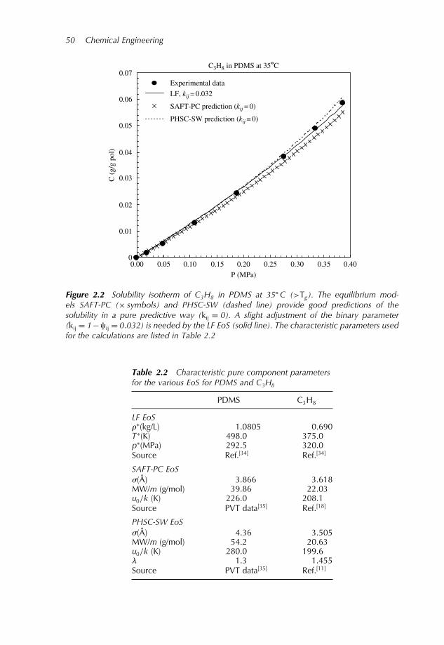
50 Chemical Engineering
C3H8 in PDMS at 35°C
0
0.01
0.02
0.03
0.04
0.05
0.06
0.07
0.00 0.05 0.10 0.15 0.20 0.25 0.30 0.35 0.40
P (MPa)
C (
g/g
pol)
Experimental data
LF, kij = 0.032
PHSC-SW prediction (kij = 0)
SAFT-PC prediction (kij = 0)
Figure 2.2 Solubility isotherm of C3H8 in PDMS at 35C (>Tg). The equilibrium mod-els SAFT-PC (× symbols) and PHSC-SW (dashed line) provide good predictions of thesolubility in a pure predictive way (kij = 0). A slight adjustment of the binary parameter(kij = 1−ij = 0032) is needed by the LF EoS (solid line). The characteristic parameters usedfor the calculations are listed in Table 2.2
Table 2.2 Characteristic pure component parametersfor the various EoS for PDMS and C3H8
PDMS C3H8
LF EoS∗(kg/L) 10805 0690T ∗(K) 4980 3750p∗(MPa) 2925 3200Source Ref.34 Ref.34
SAFT-PC EoSÅ 3866 3618MW/m (g/mol) 3986 2203u0/k (K) 2260 2081Source PVT data35 Ref.18
PHSC-SW EoSÅ 436 3505MW/m (g/mol) 542 2063u0/k (K) 2800 1996 13 1455Source PVT data35 Ref.11

Solubility of Gases in Polymeric Membranes 51
provide an extremely satisfactory representation of the sorption isotherm in the wholepressure range inspected.The second example considers a blend formed by LDPE, with 30% crystallinity, and
PVC. The polymer matrices examined are pure LDPE, the blends LDPE (80%)–PVC(20%) and LDPE (50%)–PVC (50%), and pure PVC, with toluene as the penetrant. Exper-imental data by Markevich et al.36 report solubility of toluene in the above blends, at thetemperature of 30C, while toluene solubility in pure PVC was taken from Berens37.The glassy transition temperature is equal to −25C for LDPE and to +75C for purePVC. Therefore, pure PVC is a glass at 30C; however, due to the large swelling andplasticization of the polymer induced by toluene sorption, it can be seen that the sorptionof toluene lowers the glass transition of PVC to temperatures below 30C, already atrelatively low toluene activities. That is also confirmed by the sorption isotherm which isconcave to the concentration axis as is typical of rubbery polymers. The glass transitiontemperatures for the blends are estimated to be −10C for the 80% LDPE blend and+17C for the 50% LDPE blend, all below the temperature of the sorption experiment.The crystalline fraction of LDPE is assumed, as is usual, not to contribute to the sorptionprocess, therefore we consider only the amorphous fraction of LDPE in the sorptioncalculations based on EoS. For the sake of simplicity, we present here only the resultsobtained with the LF equilibrium model.The characteristic parameters for the blend–vapor mixture are calculated with the usual
mixing rules valid for the LF EoS, by considering the blend–vapor mixture as a ternarymixture formed by the vapor and the two homopolymers. The characteristic parametersfor the pure homopolymers are shown in Table 2.3. The values of the binary adjustableparameters in the LF EoS, ij , are reported in Table 2.4. In order to fit the solubilityisotherm of toluene in pure LDPE, for this couple ij is adjusted to 0.961, while thedefault value of ij = 1 gives a good estimate of the solubility of toluene in pure PVC;the binary parameter associated with the LDPE–PVC pair has its default value. By usingthe above values of the three binary parameters, the model becomes predictive for thesolubility in the polymer blend. Comparison between experimental data and predictivecalculations is shown in Figure 2.3: as one can see, we obtain a good representationof the sorption isotherms, especially in the low-pressure range, and the dependence ofsolubility on the composition of the blend is definitely captured by the model.
2.3.3 Gas and Vapor Solubility in Glassy Polymers
Solubility isotherms of non-swelling penetrants in glassy polymers. The sorptionisotherms of CH4 in poly[phenilene oxide] (PPO) and poly[sulfone] (PSf) are now con-sidered, as well as the sorption isotherm of N2 in poly[ethylmethacrylate] (PEMA) at
Table 2.3 Characteristic pure component parametersfor the LF EoS for LDPE, PVC, and toluene
Substance ∗(kg/L) T ∗(K) p∗(MPa)
LDPE38 0883 693 400PVC38 14577 736 415Toluene39 0966 543 402

52 Chemical Engineering
Table 2.4 Binary interactionparameters for theLDPE–PVC–toluene systems
System ij
LDPE–toluene 0961PVC–toluene 1000LDPE–PVC 1000
0
0.05
0.10
0.15
0.20
0.25
0.30
0.35
0.40
0.45
0 0.001 0.002 0.003 0.004 0.005 0.006
P (MPa)
C (
g/g
pol)
LDPE
LDPE (80%)–PVC
LDPE (50%)–PVC
PVC
LF prediction
Figure 2.3 Experimental sorption data for toluene in PVC, LDPE, and their blends at30C3637. The solid lines are LF EoS correlations and predictions
the temperature of 35C 40−42, as typical examples of non-swelling penetrants. In thepractical absence of polymer dilation, only the pure component parameters and the val-ues of the unpenetrated polymer density are required for a complete description of thesolubility isotherms through the NET-GP model. The pure component parameters forthe different models used are listed in Table 2.5; they were taken from the literature orevaluated by best-fitting the EoS to the equilibrium volumetric data. The dry polymerdensity for PEMA was measured at the temperature of 25C0
pol = 1124kg/L; thevalue at 35C was thus extrapolated from volumetric data, obtaining 0
pol = 1120kg/L;for PPO at 35C, the experimental dry polymer density was taken from PVT data as1.063 kg/L, while for PSf we obtained a value of 1.230 kg/L. The values of the binaryparameters kij obtained for the various gas–polymer couples considered are listed inTable 2.6 and were adjusted on the low-pressure sorption data, according to the constantdensity assumption already recalled. The experimental data and the model calculationsare shown in Figure 2.4.

Solubility of Gases in Polymeric Membranes 53
Table 2.5 Pure component parameters for the different thermodynamic models used inthe various gas–polymer systems
Substance EoS (A) MW/m u0/k (K) References
PPO SAFT-HR 3043 2401 3200 This workPHSC-SW 3600 3773 2930 This work
PSf SAFT-HR 3043 2567 410 This workPHSC-SW 3484 3745 352 This work
PEMA SAFT-HR 3049 2298 3200 This workPHSC-SW 3450 3278 2905 This work
CH4 SAFT-HR 3700 1601 19029 9PHSC-SW 3672 1601 1649 11
N2 SAFT-HR 3575 2801 12353 9PHSC-SW 3520 2762 108 1
T∗ P∗ ∗PPO 739 479 1177 38PSf 830 600 131 24PEMA LF 602 5675 1221 This workN2 145 160 0943 21CH4 215 250 0500 21
Table 2.6 Binary parameters for the differentthermodynamic models used in the variousgas–polymer systems
Binary parameters kij
System SAFT-HR PHSC-SW SL1−ij
PEMA–N2 0020 −0018 0030PSf–CH4 −0015 −0085 −0030PPO–CH4 00 −0085 −0060
The solubility isotherms obtained from the non-equilibriummodels for all these systemsare always satisfactory and all the different models used give very similar results. Onemay notice that the worst case is represented by the PSf–CH4 systems in which the NELFmodel slightly underestimates the experimental sorption data, especially at the higherpressure range, with an error, however, not exceeding 15%.
Solubility isotherms of swelling penetrants in glassy polymers. Application of the NET-GP results to the solubility of swelling penetrants in glassy polymers is analyzed byconsidering sorption of C2 H4 in PC, of CO2 in poly[methylmethacrylate] (PMMA) andin a perfluorinated matrix. The solubility of C2 H4 in PC systems at 35C has beenexperimentally studied by Jordan and Koros43, who also measured polymer swellingduring sorption. The experimental data of sorption and dilation, together with the pre-dictions of the model, are shown in Figure 2.5. The dilation isotherm is inserted in theplot on the right-hand side of the figure, expressed in terms of polymer density versus

54 Chemical Engineering
0
0.002
0.004
0.006
0.008
0.010
0.012
0.014
0.016
0 2.5 3.0 3.5 4.0P (MPa)
C (
g/g
pol)
Experimental data
NE-SAFT-HR
NE-PHSC-SW
NE-LF
PPO–CH4
PSf–CH4
PEMA–N2
0.5 1.0 1.5 2.0
Figure 2.4 Sorption isotherm for the systems CH4–PPOCH4–PSf , and N2–PEMA; the cal-culations of different non-equilibrium models (NELF, NE-SAFT, and NE-PHSC-SW) are alsoshown
0
0.005
0.010
0.015
0.020
0.025
0.030
0.035
0.040
0 1 2 3 4 5
C (
g/g
pol)
Experimental data
NE-SAFT-HR
1.3
0 1 2 3P
ksw-exp = 0.0125MPa–1
P (MPa)
1.1
1.2ρ pol
ksw = 0 MPa–1
ksw-calc= 0.0095MPa–1
Figure 2.5 Sorption isotherm for the system C2H4–PC; the polymer dilation is reported inthe right frame in terms of polymer density versus pressure. Experimental data are from Ref.43.The results of the NE-SAFT-HR are also reported for two values of the swelling coefficientksw : experimental and calculated

Solubility of Gases in Polymeric Membranes 55
external penetrant pressure. In the present case, due to the penetrant characteristics,the swelling is not negligible and for a correct representation of the experimental datathrough the non-equilibrium models one needs to use the value of the polymer densityat each pressure during sorption, which is given by polymer dilation data.When the dilation data are readily available for the system under consideration, as
in Figure 2.5, application of the NET-GP procedure is straightforward and the modelcan be used in an entirely predictive way, provided the value of the binary parameteris known. In Figure 2.5 the predictive calculations based on NE-SAFT are presented,using the first-order approximation of the binary parameter, kij = 00. The value ofthe swelling coefficient can be calculated from the original experimental dilation data(ksw-exp = 00125/MPa) and such parameter is then used for the calculation of thesolubility isotherm.In Figure 2.5, we have also reported, for comparison, the results of the more general
procedure, which must be followed in the case, actually very frequent, in which theexperimental dilation data of the polymer are not available. According to the proce-dure illustrated in the previous section, the swelling coefficient is evaluated from oneexperimental solubility point. In the present case, the open symbol in the sorption curvein Figure 2.5 has been used to calculate the polymer volume and thus the swellingcoefficient, obtaining ksw-calc = 00095/MPa. The solubility isotherms obtained fromNE-SAFT using the experimental and calculated values of the swelling coefficient areboth shown in Figure 2.5. Clearly, the two different approaches to the solubility cal-culation give very good results. The dashed line in Figure 2.5 represents the predictionobtained by the same model neglecting swelling and assuming the polymer density isconstant during sorption and equal to the density of the pure unpenetrated polymer. Inthat case, the low-pressure behavior is in good agreement with experimental data, whileneglecting volume dilation leads to a huge underestimation of the solubility at higherpenetrant pressures. The pure component characteristic parameters for the SAFT-HREoS have been either calculated from experimental volumetric data or taken from theliterature and are reported in Table 2.7.As a further example of the applicability of the NET-GP results, we consider the
solubility of CO2 in PMMA at 33C and in Teflon® AF1600 (poly[2,2-bistrifluoromethyl-4,5-difluoro-1,3-dioxole(87%)-co-tetrafluoroethylene]) at 35C4445. For both systems,the polymer dilation data are available from independent experimental measurements,enabling us to calculate the value ksw-exp of the experimental swelling coefficient.The swelling coefficient ksw-calc has also been estimated from the solubility data byusing a single high-pressure solubility datum indicated in the figures as an open symbol.
Table 2.7 Model parameters for the systems considered in the case of swelling penetrants
Substance 0pol (kg/L) EoS Å MW/m (g/mol) u0/k (K) References
PMMA 1.181 PHSC-SW 3583 376 3669 This workCO2 PHSC-SW 2484 1626 14511 6C2H4 SAFT-HR 349 1916 21606 2
T∗ P∗ ∗AF1600 1.840 SL 575 280 2160 9CO2 SL 300 630 1515 11

56 Chemical Engineering
P (MPa)
(a)
0
0.10
0.05
0.15
0.20
0.25
0.30
0 1 2 3 4 5 6 7 8 9 10
0.91
1.1
1.21.3
0 2 4 6P
ρ pol
C (
g/g
pol)
MPa–1
ksw-calc =
0.027
MPa–1
ksw-exp =
0.026
ksw =
0.0MPa–1
Experimental data
PHSC-SW
0.01
0
0.02
0.03
0.04
0.05
0.0 0.5 1.0 1.5 2.0 2.5 3.0
P (MPa)
1.7
1.8
1.9
0 1 2 3P
(b)
ρ pol
C (
g/g
pol)
MPa–1ksw-calc
= 0.020
MPa–1ksw-exp
= 0.019
ksw =
0.0MPa–1
Experimental data
NELF
Figure 2.6 CO2 solubility in PMMA (a) at 33C and in Teflon AF1600 (b) at 35C, and thecorresponding polymer dilation isotherms are reported as a function of pressure. Experimentaldata are from Refs.4445. The results of the NE-PHSC-SW (case a) and NELF (case b) modelsare also reported for different values of the swelling coefficient ksw
The three models presented have been used for the calculations; however, for the sakeof brevity the results explicitly presented in Figure 2.6a and b refer to NE-PHSC-SW forthe PMMA–CO2 system and NELF for the AF1600–CO2 mixtures. As in the previouscase, the model results obtained with a constant polymer density value have also beenincluded in the two figures and are represented by a dashed line: once again, one can

Solubility of Gases in Polymeric Membranes 57
appreciate the importance of a correct estimation of volume dilation to account for thesorptive capacity of glassy polymers, especially at high pressure. The value of the pureunpenetrated polymer density as well as the pure component characteristic parametersused in the calculation are reported in Table 2.7, with the exception of polycarbonatewhose data were already shown in Table 2.1. From Figure 2.6a and b, we conclude thatthe models used provide a very good fitting of the experimental data, regardless of thedifferent procedure used for the estimation of the swelling coefficient and with the use of,at most, two data points. In particular, in this case we can notice the agreement betweenthe values of the swelling coefficient obtained directly from the dilation data or estimatedfrom the solubility datum: ksw-exp and ksw-calc are, respectively, equal to 0.026 and0.027/MPa in the case of the CO2–PMMA system, and to 0.019 and 0.020/MPa in thecase of the CO2–AF1600 mixtures. For CO2–PMMA mixtures, the binary interactionparameter kij was adjusted using a low-pressure solubility datum and obtaining a value of0.075, while in the case of the CO2–AF1600 mixture kij was set to its default value kij = 0.
Gas solubility in glassy polymer blends and mixed gas solubility in glassy polymers. It isworthwhile to consider now some examples of more complex systems, as polymer blendsand mixed gases, which are frequently encountered in gas separation with polymericmembranes or in barrier polymer applications. We first consider the solubility of a singlegas in glassy polymer blends and then we turn to a case of mixed gas sorption, observingthat reliable sorption data for such complex situations, in particular mixed gas sorptiondata in polymers, are rather rare in the open literature.In Figure 2.7, we report the case of two glassy polymer blends: the solubility of CH4 in
PS–TMPC (tetramethyl polycarbonate) blends of different compositions (0–20–40–60–100% of PS) is shown in Figure 2.7a at 35C46 while the solubility isotherms of CO2
in five different blends of (bisphenol-chloral) polycarbonate (BCPC) and PMMA (0–25–50–75% of PMMA)47 at 35C are shown in Figure 2.7b. The NELF estimation of thesolubility is also reported, based only on the pure component characteristic parameters
0
0.01
0.02
0.03
0.04
0.05
0.06
0.07
0 0.5 1.0 1.5 2.0 2.5
BCPC
BCPC (75%)–PMMA
BCPC (50%)–PMMA BCPC (25%)–PMMA
PMMA
NELF prediction
0
0.002
0.004
0.006
0.008
0.010
0.012
0 0.5 1.0 1.5 2.0 2.5
TMPCPS (20%)–TMPC
PS (40%)–TMPCPS (60%)–TMPC
PS
NELF prediction
P (MPa) P (MPa)
C (
g/g
pol)
C (
g/g
pol)
MPa–1ksw
= 0.005
MPa–1ksw2
= 0.019
Figure 2.7 (a) CH4 solubility in PS–TMPC blends and (b) CO2 solubility in PMMA–BCPCblends at 35C, reported as a function of pressure. Experimental data are from Refs.4647,respectively. The NELF model results are also reported as predicted on the basis of the binarysystems data alone

58 Chemical Engineering
Table 2.8 Pure polymer parameters and binary parameters for the different ternarysolutions considered
Substance 0pol(kg/L) EoS T ∗(K) P ∗ (MPa) ∗ (kg/L) References
TMPC 1.082 7616 4464 1174 23PMMA 1.188 695 560 127 21PS 1.047 LF 750 360 1099 21BCPC 1.392 794 5311 148 This workC2H4 295 345 068 21
Binary parameters kij = 1−ij
System k12 k23 k13
TMPC(1)–PS(2)–CH43 0.0 −0059 −0010BCPC(1)–PMMA(2)–CO23 0.0 −0028 −0016PMMA(1)–C2H42–CO23 0.0 0.024 0.000
and on the pure polymer sorption isotherm, which allows for the estimation of thebinary interaction parameters for the systems considered. In the case of CO2 the swellingcoefficient was also calculated. The parameters used are reported in Table 2.8, while theparameters for the blends have been calculated from those of the pure homopolymersthrough the appropriate mixing rules. The swelling coefficient of the blend is calculatedas the volume average of the pure polymer swelling coefficients, based on the volumefractions in the unpenetrated blends48. By using the swelling and binary parametersobtained from the sorption isotherms in pure polymers, calculation of solubility in theblends is entirely predictive.The two examples above show that the model allows us to predict accurately the
solubility of the blends when the pure polymer sorption isotherm for the solvent underinvestigation is known and the binary parameter associated with the polymer–polymerpair is set to its default value, as in the present cases. The results are more than satisfactory,with average errors that seldom exceed the value of 10% in the case of PS–TMPC blendsand are generally even lower for the other blends considered.The reliability of the method can also be tested in the case of mixed gas sorption in
a single glassy polymer. Also in this case a ternary mixture is present, formed by onepolymer and two low molecular weight penetrants. An example is offered by the systemPMMA–CO2–C2 H4 at 35C, studied experimentally by Sanders et al. 49, whose dataare here compared with the predictions of the NELF model. Here, the binary parametersfor both polymer-penetrant pairs were set to the default values k12 = k13 = 00, andswelling was neglected in view of the relatively low-pressure range inspected. Vapor–liquid equilibrium data for the penetrant mixture were used for the evaluation of theC2 H4–CO2 binary parameter, obtaining k23 = 0024. Therefore, again in this case theextension of the NELF to the ternary system does not require any additional adjustableparameter and the results of the model are obtained in a completely predictive mode.In Figure 2.8a and b, the CO2 and C2H4 concentration in the polymer are reported as afunction of CO2 partial pressure in the external gaseous phase, when the ethylene partialpressure is held constant at a fixed value of 206±008atm.

Solubility of Gases in Polymeric Membranes 59
0
2
4
6
8
10
12
2.5
2.0
3.0
3.5
4.0
4.5
5.00.0 1.0 2.0 3.0 4.0 5.00.0 1.0 2.0 3.0 4.0
CO2 partial pressure (atm) CO2 partial pressure (atm)
Experimental dataNE-LF
Experimental dataNE-LF
C2H
4 co
nten
t (cm
3 STP/
cm3 )
CO
2 co
nten
t (cm
3 STP/
cm3 )
Figure 2.8 (a) C2H4 and (b) CO2 concentration in a ternary PMMA–C2H4–CO2 mixtureas a function of CO2 partial pressure. The ethylene fugacity in the vapor phase was heldconstant during the measurements. The solid line represents the NELF prediction based onthe binary mixtures data. Experimental data are from Ref.49
As in the previous cases, the non-equilibrium model gives quite good results in pre-dicting the experimental data; the ethylene content is in fact very well calculated and theslight underestimation of the CO2 content at the higher penetrant partial pressure can beattributed to the polymer swelling that probably occurs in such a condition and whichhas been neglected in the calculation.
2.4 Conclusions
The solubility of low molecular weight penetrants in polymeric matrices can be satisfac-torily calculated by using several EoS models such as LF, SAFT-HR, and PHSC-SW.For rubbery phases, the models are used in their original equilibrium formulations,
which requires knowledge of the pure component parameters and the binary interac-tion parameters entering the mixing rules associated with the models. The former canbe retrieved from pure component volumetric data at different temperatures and pres-sures and, when applicable, from vapor pressure data; for each pair of substances thebinary parameter is either retrieved from volumetric data or adjusted to the solubilitydata. In several cases, the default value offers a reasonable estimation of the solubilityisotherms.In the case of glassy polymers, on the other hand, the equilibrium approach is not
applicable and a suitable non-equilibrium thermodynamic approach has been developed,NET-GP, which indicates how the selected free energy model can be extended to non-equilibrium glassy phases offering, in particular, explicit expressions for the penetrantchemical potential in glassy polymers. The departure from equilibrium is lumped into theglassy polymer density which is the only additional information that is needed, beyondthe parameters used for the equilibrium rubbery phases. The model is fruitfully applied tothe cases of non-swelling and swelling penetrants, as well as for calculating the solubilityin polymer blends and of mixed gases.

60 Chemical Engineering
Acknowledgements
This work has been partially supported by the University of Bologna (progetto pluriennale2004–06 and ‘60% funds’).
References
[1] Flory P.J. 1941. J. Chem. Phys., 9, 660.[2] Huggins M.L. 1941. J. Chem. Phys., 9, 440.[3] Abrams M.M. and Prausnitz J.M. 1975. A.I.Ch.E J., 21, 116.[4] Oishi T. and Prausnitz J.M. 1978. Ind. Eng. Chem. Res., 17, 333.[5] Elbro H.S., Fredenslund A. and Rasmussen P. 1990. Macromolecules, 23, 4707.[6] Patterson D. 1969. Macromolecules, 2, 672.[7] Flory P.J. 1970. Disc. Faraday Soc., 49, 7.[8] Sanchez I.C. and Lacombe R.H. 1978. Macromolecules, 11, 1145.[9] Huang S.H. and Radosz M. 1990. Ind. Eng. Chem. Res., 29, 2284–2294.[10] Song Y., Hino T., Lambert S.M. and Prausnitz J.M. 1996. Fluid Phase Equilib., 117, 69–76.[11] Hino T. and Prausnitz J.M. 1997. Fluid Phase Equilib., 138, 105–130.[12] Kang J.W., Lee J.H., Yoo K.P. and Lee C.S. 2002. Fluid Phase Equilib., 194, 77–86.[13] Sanchez I.C. and Lacombe R.H. 1976. J. Phys. Chem., 80, 2352–2362.[14] Lacombe R.H. and Sanchez I.C. 1976. J. Phys. Chem., 80, 2568–2580.[15] Sanchez I.C. and Lacombe R.H. 1977. J. Polym. Sci.: Polym. Lett. Ed., 15, 71–75.[16] Chapman W.G., Gubbins K.E., Jackson G. and Radosz M. 1989. Fluid Phase Equilib., 52, 31.[17] Chapman W.G., Gubbins K.E., Jackson G. and Radosz M. 1990. Ind. Eng. Chem. Res.,
29, 1709.[18] Gross J. and Sadowsky G. 2001. Ind. Eng. Chem. Res., 40, 1244.[19] Song Y., Lambert S.M. and Prausnitz J.M. 1994. Macromolecules, 27, 441.[20] Doghieri F. and Sarti G.C. 1996. Macromolecules, 29, 7885.[21] Sarti G.C. and Doghieri F. 1998. Chem. Eng. Sci., 53, 3435–3447.[22] Doghieri F., Canova M. and Sarti G.C. 1999. Polymer membranes for gas and vapor sepa-
rations, ACS Symp. Ser., 733, 179–193.[23] Giacinti Baschetti M., Doghieri F. and Sarti G.C. 2001. Ind. Eng. Chem. Res., 40, 3027–3037.[24] Doghieri F. and Sarti G.C. 1998. J. Membr. Sci., 147, 73.[25] Coleman B.D. and Gurtin M.E. 1967. J. Chem. Phys., 47, 597.[26] Koros W.J., Paul D.R. and Rocha A.A. 1976. J. Polym. Sci.: Polym. Phys. Ed., 14, 687.[27] Koros W.J. and Paul D.R. 1978. J. Polym. Sci.: Polym. Phys. Ed., 16, 1947.[28] Fleming G.K. and Koros W.J. 1990. Macromolecules, 23, 1353.[29] Wang J.S. and Kamiya Y. 2000. J. Polym. Sci., Part B: Poly. Phys., 38, 883.[30] Colina C.M., Hall C.K. and Gubbins K.E. 2002. Fluid phase equilib., 194–197, 553–565.[31] Hariharan R., Freeman B.D., Carbonell R.G. and Sarti G.C. 1993. J. Appl. Polym. Sci., 50,
1781–1795.[32] Kiszka M.B., Meilchen M.A. and McHugh M.A. 1988. J. Appl. Polym. Sci., 36, 583–597.[33] Pope D.S., Sanchez I.C., Koros W.J. and Fleming G.K. 1991. Macromolecules, 24,
1779–1783.[34] De Angelis M.G., Merkel T.C., Bondar V.I., Freeman B.D., Doghieri F. and Sarti G.C. 1999.
J. Polym. Sci., Polym. Phys. Ed., 37, 3011–3026.[35] Zoller P. and Walsh D. 1995. Standard Pressure–Volume–Temperature Data for Polymers.
Technomic, Lancaster.[36] Markevich M.A., Stogova V.N. and Gorenberg A.Ya. 1991. Polym. Sci. USSR, 1, 132–140.

Solubility of Gases in Polymeric Membranes 61
[37] Berens A.R. 1985. J. Am. Water Works Assoc., 77(11), 57–64.[38] Rodgers P.A. 1993. J. Appl. Polym. Sci., 48, 1061.[39] Sanchez I.C. and Panayiotou C. 1994. In, Models for Thermodynamic and Phase Equilibria
Calculations, Sandler S.I. (Ed.). Dekker, New York, pp. 187–285.[40] Chiou J.S. and Paul D.R. 1989. J. Membr. Sci., 45, 167.[41] Davydova M.B. and Yampolskii Yu. P. 1991. J. Polym. Sci. USSR, 33, 495.[42] McHattie J.S., Koros W.J. and Paul D.R. 1991. Polymer, 32, 840.[43] Jordan S. and Koros W.J. 1995. Macromolecules, 28, 2228.[44] Wissinger R.G. and Paulaitis M.E. 1991. Ind. Eng. Chem. Res., 30, 842.[45] De Angelis M.G., Merkel T.C., Bondar V.I., Freeman B.D., Doghieri F. and Sarti G.C. 2002.
Macromolecules, 35, 1276.[46] Muruganandam N. and Paul D.R. 1987. J. Polym. Sci., Part B: Polym. Phys., 25, 2315.[47] Raymond P.C. and Paul D.R. 1990. J. Polym. Sci., Part B: Polym. Phys., 28, 2103.[48] Grassia F., Giacinti Baschetti M., Doghieri F. and Sarti G.C. 2004. Advanced materials for
membrane separations, ACS Symp. Ser., 876, 55–73.[49] Sanders E.S., Koros W.J., Hopfenberg H.B. and Stannett V.T. 1984. J. Membr. Sci., 18, 53.

3Small Peptide Ligands for AffinitySeparations of Biological Molecules
Guangquan Wang, Jeffrey R. Salm, Patrick V. Gurgel and Ruben G. Carbonell
3.1 Downstream Processing in Biopharmaceutical Production
The biotechnology industry faces serious challenges to profitability1. Since downstreamprocessing accounts for 50–80% of the cost of manufacturing a therapeutic product,reductions in the number of steps in the purification train and increases in the yieldand purity of the product in each step would effectively decrease production costs. Inaddition, there is a shift among regulatory agencies to what are called ‘well-characterizedbiologics’, which require that all manufactured biological products be essentially free ofcontaminants.A typical industrial process for recovery and purification of therapeutic proteins or
other biological molecules from fermentation broths or mammalian cell culture mediaoften involves a complex series of steps. In the simplest case of a product excreted froma cell into a culture medium, the cells must first be separated from the broth by filtrationor centrifugation. A rough separation step such as precipitation with ammonium sulfatefollowed by filtration can lead to a significant concentration of the desired protein incombination with other contaminants. A re-suspension of this precipitate can then beprocessed over a series of ion exchange columns for higher purification, followed bya polishing step using gel permeation chromatography. In a case where the product isbound to inclusion bodies or membranes within the cell, the purification is more complex,often involving the addition of chaotropic solvents and refolding of the protein into itsactive conformation. The large number of steps required to separate and purify biologicalmolecules often results in significant losses of product yield and activity. For this reason,increasing attention is being given to affinity chromatography as a purification method
Chemical Engineering: Trends and Developments. Edited by Miguel A. Galán and Eva Martin del ValleCopyright 2005 John Wiley & Sons, Inc., ISBN 0-470-02498-4 (HB)

64 Chemical Engineering
that would result in both a reduction in the number of steps required for purification aswell as a higher yield of product mass and activity.
3.2 Affinity Chromatography
In affinity chromatography, a ligand that is able to bind the target molecule specificallyfrom a mixture is attached to a porous chromatographic support with suitable flowproperties and binding capacity. As shown in Figure 3.1, the mixture containing thedesired product is injected into the column, resulting in the adsorption of the target specieson the chromatographic support. This adsorption step is continued until the column issaturated with the desired product and the solution begins to show a small amount ofbreakthrough of the product at the outlet. At this point, a washing buffer is introducedto remove from the resin any material that is bound non-specifically. Typically, thiswash is carried out with a buffer with a slightly elevated ionic strength containing weakdetergents. Once the contaminants are removed, an elution buffer of low or high pH orionic strength, perhaps containing chaotropic solvents, is injected to remove the productfrom the chromatographic support in a concentrated and highly pure form. After severalcycles of use, it is necessary to wash the column with acid or basic solutions in order toremove any pathogens or residual material that might contaminate the product.To execute a successful affinity chromatography separation, the ligand must bind
strongly enough to the product so that it will be able to selectively adsorb and concentrateit from the mixture. However, it cannot bind so strongly that harsh solvents are neededfor elution thus reducing the product activity. Ligands with association constants equalto or higher than 106/M are generally preferred for this purpose. Finally, the capacityof the resin should be sufficiently high so that the column dimensions (and cost) arein a reasonable range. Capacities can range anywhere from 2 to 30mg of product per
FeedImpurities
Target molecule
Adsorption Wash
Washbuffer
Elution
Elutionbuffer
Ligand
Resin
Figure 3.1 Schematic representation of affinity chromatography. The adsorption step iscontinued until the column is saturated. A wash step removes unwanted impurities bound tothe resin. Elution of the product is executed by changing buffer conditions

Small Peptide Ligands for Affinity Separations 65
milliliter of resin. There are many ligands for affinity chromatography that exploit nature’smethods for molecular recognition. These include inhibitor–enzyme, receptor–protein,oligonucleotide–protein, and antigen–antibody pairs. Other naturally occurring biologicalmolecules such as heparin and Protein A can do an excellent job of separating andpurifying proteins from complex mixtures. Of these, the use of antibodies as affinityligands for chromatography has been found to be the most flexible, especially in laboratoryapplications. Since either monoclonal or polyclonal antibodies can be generated againstjust about any biological molecule, literally thousands of purification processes rely onantibodies as the preferred ligands for affinity purification on a small scale.Affinity chromatography is a very well established technique, whose roots can be traced
to the work of Cuatrecasas, Wilchek, and Anfinsen in 19682. Between the years 1994and 1996 alone, over 150 patents per year were awarded using affinity chromatographyas the method of choice for purification, and over 60% of the purification protocolspublished involve affinity chromatographic steps somewhere in the process3. Given thislevel of research activity, one would think that affinity chromatography steps would becommon in the bioprocess industry, but this is not the case. There are many challengesto the establishment of affinity chromatography as a method of choice for industrialseparations. The section that follows discusses some of these challenges and how smallpeptide ligands can play in a role in overcoming them4−8.
3.3 Advantages of Small Peptide Ligands
The high cost of monoclonal or polyclonal antibodies often makes the use of affinitychromatography for any large-scale separation prohibitively expensive. For therapeuticproducts, the affinity ligand must be extremely well characterized, and it must have apurity that rivals that of the product itself. As a result, the mere production of the highlypure monoclonal or polyclonal antibody ligand results in a significant cost of generatingthe chromatographic support. In addition, all methods of immobilization or attachmentof the antibody to the support result in some leakage of the ligand into the product withcolumn use. In the case of production of therapeutics, this leakage needs to be carefullymonitored and steps need to be introduced to remove small amounts of the antibody fromthe product solution. Failure to do this can result in immunogenic reactions in the patientcaused by the presence of foreign animal proteins.The elution and wash steps that are necessary in affinity chromatography can result in
a reduction in the affinity of the antibody for the target molecule. Since antibodies areproteins that recognize other molecules as a result of their tertiary structure in solution,any solvent changes that result in small modifications of tertiary structure can causereductions in affinity. Repeated numbers of adsorption, elution, and column cleaningcycles can deactivate what started as a highly effective but extremely expensive column.In addition, the binding of many antibodies to the product species is so specific andstrong that rather extreme elution conditions are necessary for product recovery, resultingin loss of activity.Regardless of the ligand type, chromatographic supports must be tested and validated
against ligand leakage, binding of pathogens such as endotoxins and viruses, and forrobust yield and purity results after being subjected to a large number of cycles of use.A great deal of work has been done on small organic ligand (including dyes) affinity

66 Chemical Engineering
chromatography and immobilized metal affinity chromatography (IMAC). Small organicmolecule ligands and immobilized metal ions are more stable and less expensive thanantibodies so that they can stand harsh operation conditions, but neither of them exhibitgreat selectivity when exposed to a complex mixture, unless the organic is speciallydesigned to adsorb to a specific site on the surface of the protein. In addition, dye ligandsand metal ions may be toxic and with metal ligands in particular, there is a problemwith severe leakage from the support. There are small organic molecules currently incommercial use as ligands for the industrial purification of proteins, and some of themore successful ones involve triazine derivatives3.
Peptides with anywhere from 3 to 25 amino acid residues can have affinities tomolecules of interest that compare well with dyes, immobilized metal ions, and someantibodies. As opposed to monoclonal antibodies, small peptide ligands are much morestable because they do not require a specific tertiary structure to maintain their activity.Small peptides are also less likely than an antibody to cause immune response in case ofleakage into the products. Peptides can be manufactured aseptically in large scale underGMP (good manufacturing practices) conditions at relatively low cost compared withantibodies, especially if they have less than 13 amino acids. The interactions betweenpeptides and proteins are moderately strong so that the protein can be eluted undermild conditions without loss of protein activity. In addition to being good candidates asligands in affinity chromatography, peptides are used widely to determine protein–proteininteractions without a priori information on protein structure (e.g. in epitope mapping).The identification of suitable peptide ligands for a given separation is often carried out
using combinatorial peptide libraries generated with phage, yeast, ribosome, and otherdisplay vehicles. A great deal of work has been done with libraries of peptides contain-ing 13–58 amino acids, multimeric or geometrically constrained peptides, Affibodies™,single-chain variable fragments of antibodies, etc. Because of the relatively large size ofthese peptides, the binding is often also determined by the three-dimensional configura-tion of the ligand, and as a result, these would be subject to the same stability difficultiesexperienced with whole antibodies. In addition, peptides with 13 or higher numbers ofamino acid residues are very expensive to produce using synthetic routes, and must beproduced by expression in recombinant organisms. As a result, little significant costsavings ensue from making a large peptide as opposed to a full antibody. Nevertheless,several groups have been actively pursuing this approach with some success, includingTecnogen in Milan, Affibody AB, Dyax, and Amersham Biosciences.Our group has worked on an alternative approach based on the use of small pep-
tides (three to eight amino acids) as ligands for affinity chromatography. For thecase of peptides of this size it is possible to generate very large combinatorial pep-tide libraries on solid phase supports that are chromatographic resins. For example,over 34 million hexamers can be generated with 18 of 20 naturally occurring aminoacids (excepting cysteine and methionine), each on a different resin bead, using onlyabout 18 g of chromatographic resin. Using appropriate screening techniques, it is possi-ble to isolate and sequence a very small number of leads that can then be studied furtherto verify binding to the target species. Since the peptides are already attached to thedesired chromatographic support, they can then be made on a larger scale to generatethe chromatographic column. It often happens that a peptide that can bind to a protein insolution or on the surface of a phage does not bind when immobilized on a solid support.The screening approach used in our work eliminates this possibility. Finally, when small
Small Peptide Ligands for Affinity Separations 67
peptides leak from a column they have a smaller chance of producing an immunogenicresponse, and since they do not exhibit a precise tertiary structure, their binding charac-teristics are not highly affected by solvents used in repeated cycles of adsorption, elution,and cleaning of the support. As opposed to antibodies, whose association constants with atarget on a solid support can be 109–1010/M, small peptides exhibit association constantsaround 106–108/M. These weaker association constants allow for relatively gentle elutionconditions, higher product activity yields, and better column longevity.Baumbach and Hammond first demonstrated the principle of using small peptide lig-
ands from combinatorial libraries as affinity ligands in large-scale chromatography pro-cesses by using streptavidin as a target4. Since then, this technique has been successfullyused to purify a variety of proteins, such as s-protein6, von Willebrand factor7, factorIX9, factor VIII10, trypsin11, anti-MUC1 antibodies1213, -1-proteinase inhibitor5,monoclonal antibodies (IgG, IgA, IgE, IgM, IgY)14, -lactalbumin1516, fibrinogen17,and staphylococcal enterotoxin B (SEB)18.In this chapter, we will try to summarize aspects of the construction and screening
of combinatorial libraries of small peptides, the nature of the protein–ligand interactionson these supports, the effects of peptide density on performance, and the factors thatdetermine the dynamic binding capacity of the resins. The concluding section will mentionsome of the current areas of investigation on novel applications for this promisingtechnology.
3.4 Combinatorial Peptide Libraries
3.4.1 Phage-Displayed Libraries
One of the challenges for the use of peptide ligands in affinity chromatography is theidentification of a sequence that shows affinity and specificity to the target protein.Examples in the literature show that designing a specific complementary peptide sequenceis difficult even when the structure of the target protein is known1920. The developmentof combinatorial libraries has allowed the screening of millions of peptide sequencesto discover specific peptides that bind to the target protein. Peptide libraries can begenerated either biologically or synthetically. Several combinatorial library methodshave been described in the literature21. The most widely used biological libraries arephage-displayed libraries, while one-bead-one-peptide libraries are the dominant librariesobtained directly from chemical synthesis.In phage-displayed peptide libraries, random oligonucleotides with a given length are
generated and then inserted into bacterial phage gene III. The corresponding peptidecoded by the inserted DNA is displayed at the N-terminal of the gene III protein (pIII)on the phage surface. Each phage displays one peptide sequence that is different fromthose on other phages. Affinity peptides on phage that bind to the target protein areselected through several rounds of affinity purification. Millions of phage particles areincubated with the target protein immobilized on a Petri dish or ELISA plates. Non-binding phages are washed out extensively, and then the bound phages are eluted underharsh conditions. The eluted phages are then amplified on agar medium and subjected
68 Chemical Engineering
to the next round of affinity purification. The tight-binding phages are then cloned andpropagated in Escherichia coli. The amino acid sequence of the peptide on the phage isdeduced by sequencing the coded DNA in the phage gene III22−24.
Ligands identified from phage libraries frequently interact with natural binding siteson the target molecule and resemble the target’s natural ligands. Thus phage-displayedrandom peptide libraries have been used to investigate protein–protein interactions in avariety of contexts. For example, phage-displayed random peptide libraries have beenused to map the epitopes of monoclonal and polyclonal antibodies, and to identify peptideligands for receptors, receptor ligands, and folded domains within larger proteins, suchas several SH2, SH3 domains2526. Recently, peptide ligands for some superantigens, forexample, SEB and TSST-1, have been determined with phage-displayed random peptidelibraries2728. However, biopanning with phage-displayed libraries is slow and subjectto non-specific binding.Phage-displayed random peptide libraries have been constructed to display peptides
of variable length ranging from 6 to 38 amino acids25. Phage display libraries have theadvantage of allowing exposure of very large peptides as potential ligands. Once it iscreated, a phage library can be regenerated continuously and re-used unlike a syntheticlibrary. Usually the diversity of the original phage library is on the order of 108 peptides.Selection must be avoided during the library expansion and propagation for phages withselective growth advantage25. Peptide synthesis on phages is limited to the 20 naturalamino acids so that d-amino acids or other molecules cannot be used to increase thediversity of the library.
3.4.2 One-Bead-One-Peptide Libraries
Synthetic libraries can be created on solid supports through organic chemistry. Thereare several distinct combinatorial library methods21. The one-bead-one-peptide librarymethod is used extensively in drug discovery processes due to its unique features29.Compared with other methods, the synthesis of a one-bead-one-peptide library is rapidwith use of the ‘split synthesis’ approach. Because one bead has one unique peptidesequence, all of the beads can be tested concurrently but independently. Once positivebeads have been identified, the chemical structure of the peptides on the beads can bedirectly determined by sequencing or by an encoding strategy. In addition, the libraries canbe used either in the solid phase (i.e. peptides attached on solid) or in the solution phase(i.e. peptides cleaved from solid support). As in phage-displayed libraries, the screening ofpeptide ligands from one-bead-one-peptide libraries involves three steps21: constructionof the library, screening the library with the target molecule, and determination of thepeptide sequence.Although peptide ligands from phage library have been presented on chromatographic
support to purify proteins467, it is possible that the microenvironment and the orientationof the peptides on the chromatographic support could be very different from that onphage. This can adversely affect the interactions between the peptide ligands and thetarget9. It has been found that some peptides derived from a phage library work onlywhen the peptide is an integral part of the phage coat protein and not when isolated infree solution or on a solid support1. Thus one-bead-one-peptide libraries are uniquelysuited to discover peptide ligands for protein purification.

Small Peptide Ligands for Affinity Separations 69
3.4.3 Libraries on Chromatographic Resins
To avoid the possibility that a small peptide from a phage-displayed library will not bindadequately when immobilized on a solid support, Baumbach and Hammond suggestedthat combinatorial peptide libraries for protein purification be synthesized directly onresins that could be used as chromatographic supports on a large scale4. In this way,any ligand that is identified is already on a platform or format that would facilitateimplementation in downstream processing. The one-bead-one-peptide solid phase libraryformat is ideally suited for this purpose, if the library is built on chromatographic resinsthat can withstand the harsh solvent conditions used for peptide synthesis.The first one-bead-one-peptide library was synthesized by Lam et al.30 using the ‘split
synthesis’ approach pioneered by Furka and Sebetyen31. Figure 3.2 shows how thisapproach is implemented in library construction. The resin beads are divided equallyinto separate reaction vessels of an automatic peptide synthesizer, each with a singleamino acid. After the first amino acid is coupled to the resins, beads are repooled, mixedthoroughly, and redistributed into separate reaction vessels. The next coupling step isthen performed. This divide–couple–recombine technique is repeated until the desiredlength of the peptide library is reached. There are Xn random sequences in the library,where X is the number of amino acids used for coupling and n is the length of the library.If X is the total number of natural amino acids (20) and n= 6 (hexamer library), the totalnumber of different peptides generated is 64 million. Each resin bead displays multiplecopies of only one peptide sequence. Thus libraries of this type are called ‘one-bead-one-peptide’ libraries30. Because other ligands besides naturally occurring amino acids, suchas d-amino acids, oligonucleotides, synthetic oligomers, proteins, and small molecules,also can be coupled to solid resins, the idea of a one-bead-one-peptide library has beenextended to one-bead-one-compound library21. The introduction of other compoundsbesides amino acids in combinatorial library construction increases the diversity of thelibrary in comparison with a phage-displayed peptide library, in which phages only
• Synthetic peptide library constructed using ‘divide, couple, recombine’ technique• Stepwise synthesis using F-moc and t-Boc solid phase chemistry and 18 of 20 naturally occurring L-amino acids (except Cys and Met)• Method generates 34 × 106 unique peptide hexamers• Peptide density ~100 µ moles/g Chromatographic
resin
A B C
AA, AB, AC BA, BB, BC CA, CB, CC
AAA, AAB, AAC BAA, BAB, BAC CAA, CAB, CACABA, ABB, ABC BBA, BBB, BBC CBA, CBB, CBC
CCA, CCB, CCCBCA, BCB, BCC ACA, ACB, ACC
Divide
Couple
Recombine
Figure 3.2 Construction of a one-bead-one-peptide library. For N amino acids in the library,repetition of the split synthesis technique n times results in Nn different peptides in the library

70 Chemical Engineering
display peptides composed of natural amino acids. However, all synthetic methods havea practical limit on the size of the library as well as the length of the peptides on beads,while peptides on phage can be fairly large.The choice of the solid support is critical for the library construction and the application
of the library. The biological signal released from the peptides on a single bead dependsquantitatively on the amount of the peptide on the bead. As a result, the size andsubstitution homogeneity is of the utmost importance. Meanwhile, the resin should resistthe formation of clusters because clusters would prevent the statistical distribution of resinbeads and lower the number of structures created. In addition, resins should be compatiblewith various organic and aqueous media. Solid beads with porous structure are preferred.The high surface area provided by porous resin results in a high ligand concentration,facilitating bead sequencing and providing high capacity for their use in chromatography.Moreover, the pores should be large enough to reduce diffusion resistance especially whenusing large proteins as targets. In order to avoid non-specific binding between the solidmatrices and proteins, hydrophilic resins are preferred. If the peptide ligands will be usedto purify protein in chromatography, the resins should have enough mechanical rigidityto withstand the high pressure used in liquid chromatography. A variety of polymer beadshave been used to attach peptides in library construction, including polyhydroxylatedmethacrylate, polydimethylacrylamide, polyoxyethylene-grafted polystyrene, Tentagel,and so on921.The solid phase library used in the majority of the work done in our lab is constructed
on Tosoh BioSciences, Inc. Toyopearl AF Amino 650 M resin as shown in Figure 3.3.Toyopearl resin is a functionalized hydroxylated polymethacrylate resin that works wellwith the F-moc and t-Boc chemistries used for peptide synthesis. The peptides aresynthesized directly on the primary amines on the end of hydrophilic spacer arms that areattached to the resin surface. Toyopearl resin is also mechanically and chemically stablewhich allows it to be scaled up into a commercial setting. This resin has a maximumcoupling density of approximately 400moles of ligand per gram of dry resin, and ininternal surface area of approximately 30m2/g. Libraries of these materials are normally
• Tosoh Biosciences ToyoPearl amino resin (400 µ moles/g)• Hydroxylated methacrylate base resin• Chemically and mechanically stable• Average pore size: 100 nm; particle size: 40–90 µ m• Total surface area: 30 m2/g of resin
Typical peptidedensity
~100 µ moles/g51 Å2/molecule
8 Å
Region of influence ofa peptide
NH
–A–X
–X–X
–X–X
–X–N
H2
NH
–A–X
–X–X
–X–X
–X–N
H2
NH
–CO
–CH
3
NH
–CO
–CH
3
NH
–CO
–CH
3
NH
–CO
–CH
3
NH
–CO
–CH
3
NH
–CO
–CH
3
Linker: –O–R–O–CH2–CHOH–CH2–
+ +
Figure 3.3 Properties of Toyopearl library support and ligand structure

Small Peptide Ligands for Affinity Separations 71
synthesized with a peptide density of approximately 100moles/g, and any uncoupledprimary amines should be acetylated to reduce non-specific binding of target proteins. Atthis peptide density, the individual peptides are separated from each other by roughly 8 Å.The average pore size of 1000 Å and the large porosity of the resin make the poresaccessible even to fairly large protein targets. These 65-m-diameter resins are meantfor large-scale chromatographic separations since they are rigid and exhibit excellentflow and chemical properties. As a result, the libraries created from these resins resultin the identification of a peptide that binds to the target species and is already attachedto a chromatographic support. This helps to eliminate any situations where a peptidemight be identified using a phage-displayed library and not bind when attached to achromatographic support. A hexamer library constructed on Toyopearl with 18 aminoacids will weigh approximately 18 g of dry resin, which, when swollen in methanol,will occupy a volume of roughly 84.6mL. Phage-displayed libraries can generate fulldiversity of very large peptides that cannot be achieved with the solid phase librariessince the amount of resin and amino acids required for chemical synthesis would makethem prohibitively large and expensive.
3.5 Screening of One-Bead-One-Peptide Libraries
3.5.1 On-Bead Binding Screening
Both solid phase and solution phase methods have been used for screening one-bead-one-peptide combinatorial libraries. The most widely adopted method of screening is the‘on-bead’ binding assay2132. The target protein is incubated with the library, so that theprotein can bind to beads that have specific peptide sequences favorable for adsorption.The binding of the target to the immobilized ligands is usually detected by using a reportergroup such as an enzyme, a radionuclide, a fluorescent probe, or a color dye covalentlyattached to the target molecules. Alternatively, immunodetection schemes such as inenzyme-linked-immunosensitive assays (ELISA) can be used to detect binding to a resinbead. The signals generated from these reporter groups are proportional to the amount anddensity of peptides on the beads, as well as the size of the beads. Non-specific binding canresult in high background with both immunodetection as well as direct detection methods,generating some difficulty in determining which beads contain true affinity ligands. Thisis usually eliminated by using blocking proteins (e.g. casein or bovine serum albumin),by washing with a high ionic strength buffer (e.g. 0.2–0.4M NaCl) to reduce purelyelectrostatic binding, and by washing with nonionic detergents (e.g. 0.1% Tween 20).One of the most convenient screening methods is the enzyme-linked colorimetric
detection scheme. It has been used to discover the binding motifs for streptavidin3033,avidin33, monoclonal antibodies34, proteases34, and MHC molecules35. The enzyme-linked colorimetric detection method is extremely rapid, taking a few hours to screen107–108 beads. The problem with this method is that the enzyme molecule attached tothe target can sterically affect the binding of the target to peptides on beads.Radionuclide-labeled targets can be used to screen library beads to avoid this problem.
The radionuclide probes, such as 3H and 14C, are particularly small compared with enzymeas reporter groups on the target, and it has been demonstrated that the labeled targetshows almost the same biological properties as the natural target36. A schematic diagram

72 Chemical Engineering
• Solid-phase, ‘one-bead, one peptide’ library of hexamers H2N–X–X–X–X–X–X–A–Linker–Tosoh Biosciences amino resin
1. Block librarywith target stream
2. Incubate librarywith radiolabeledtarget
3. Wash library
4. Suspend librarybeads in agarose asmonolayer
5. Expose tofilm
6. Develop film
7. Match geland film
8. Excise beads forsequencing byEdman degradation
X-ray filmGel withbeads
+
Figure 3.4 Radiological screening of a hexamer peptide library by the method of Mondorfet al38
of the process is shown in Figure 3.4. The library is incubated with the radiolabeledtarget protein, washed, and then suspended in agarose gel. The slurry is poured onto a gelbond to form a monolayer so that all beads are spatially separated. Exposure of the gel toautoradiography film can locate the positive beads that are then isolated and sequenced.Several researchers have screened peptide libraries using radiolabeled targets37−40. Themethod developed by Mondorf et al.38 using 14C offers high resolution and sensitiv-ity. It has been used to identify affinity peptide ligands for s-protein38, fibrinogen38,-1-proteinase inhibitor5, -lactalbumin15, recombinant factor VIII41, and SEB18.Immunostaining schemes similar to ELISA also can be used to target the protein
on beads. There are no modifications of the target using this method, so the bead-bound ligands bind directly to the native protein, and not to any adducts. However, theantibodies used in the detection system could bind to bead-bound ligands other than thetargets to bring the possibility of interference and false positives. A two-color PEptideLibrary Immunostaining Chromatographic ANalysis (PELICAN) has been developed todetermine beads specifically for the target from those beads resulting from antibodycross-reactivity9. It has been used to discover peptide leads for protease factor IXand fibrinogen942. Other on-bead screening schemes involve dye-labeled targets orfluorescently labeled target4344. However, dyes always complicate the screening processby binding directly to many peptide ligands, and the autofluorescence of the librarymakes it unsuitable for this kind of screening process21.
In order to minimize the number of false positive beads and make the screeningmore selective, two different screening methods can be sequentially used for one target.For example, a dual-color detection scheme that uses two sequential orthogonal probesin enzyme-linked colorimetric detection methods45 and a cross-screening scheme thatcombines an enzyme-linked colorimetric method and a radiolabeled assay46 have beendeveloped. In this way, many of the initially determined positive beads are eliminatedby the second screening method, and the chances of getting the true positive beads aregreatly enhanced.

Small Peptide Ligands for Affinity Separations 73
3.5.2 Screening of Soluble Combinatorial Peptide Libraries
One of the disadvantages of on-bead screening is the high peptide density required forpeptide sequencing on beads. This can lead to multiple-point attachment of the targetto the peptides so that non-specific interaction between target and peptides will beenhanced. Thus the selected peptide ligands may have less affinity and specificity tothe target. Screening of soluble peptide libraries can make the affinity ligands moreselective. The format of affinity chromatographic screening developed by Evans et al.47
and Huang and Carbonell8 is suitable for screening peptide libraries due to its rapidity.The targets are immobilized onto resins and then packed into a chromatographic column.The soluble peptide libraries are pumped into the column at a proper flow rate to ensure thepeptides have enough time to bind to the immobilized targets. Then the column is washedthoroughly with binding buffer. The affinity peptide ligands bound to the targets are elutedand then isolated by reverse-phase chromatography. The fractions are then sequenced byEdman degradation or mass spectrometry. Huang and Carbonell have demonstrated thistechnique by showing that the identified sequence consensus, NFVE, is the same as thatfound from screening a phage-displayed library for s-protein8. Evans et al.47 used asimilar system to recover the known epitope, YGGFL, for a monoclonal antibody (3E-7),and then determine the affinity ligands for bacterial lipopolysaccharide (LPS, endotoxin).Although this technique is rapid and able to avoid false signals from non-specific binding,some hydrophobic leads could be missed due to their minimal solubility. The slowbinding kinetics and the orientation of the immobilized targets may limit the contactbetween the immobilized targets and the free peptide ligands so that some potential leadscould pass through the column. In addition, the methodologies used in this technique aremore complex than those in on-bead screening8.
3.5.3 Multi-Tiered Screening
A multi-tiered screening process was developed to help identify and eliminate falseleads from the solid phase library screenings in our work51518 as shown in Figure 3.5.
Primaryscreening
Secondaryscreening
Tertiaryscreening
Approximately 105 compoundsRadiological screeningPure target protein
Approximately 10–20 leadsResynthesized on resin (1 gm) Batch binding experimentsPure protein, simple mixtures2% acetic acid elution
Approximately 2–3 leadsResynthesized on resinChromatographic formatActual feed streamOptimized elution conditionsOptimized peptide density
PurityYieldStability
Figure 3.5 Multi-tiered screening process. The path from primary to tertiary screeningfocuses the final sequence that gives the best combination of purity and yield in purification

74 Chemical Engineering
The ‘primary screening’ process involves identification of leads that are thought to bindspecifically to the target protein. ‘Secondary screening’ is used to confirm the bindingof the target protein to a larger mass of resin that contains the peptide ligands identifiedduring the primary screening in a non-competitive format. Some peptides that boundweakly to the target protein are eliminated during secondary screening. The ‘tertiaryscreening’ process is performed in a column format to demonstrate the binding selectivityof the peptide ligands for the target protein from its native feed stream.Since the largest amount of time in lead discovery is often spent on characterizing
the one or two leads that are eventually shown to bind the target, considerable resourcescan be saved by decreasing the 20 or so leads identified during primary screening downto 4 or 5 leads for detailed characterization. Once leads from primary screening aresequenced, larger batches (1 g) of resin with each of the leads are re-synthesized to beused in secondary screening. Batch experiments with pure protein are carried out to verifybinding of the target protein to the different peptide leads. From 20–30 beads in primaryscreening, only a few might show sufficient protein adsorption to move toward tertiaryscreening. In tertiary screening, issues such as the elution conditions and binding buffersused with the peptide are optimized to increase yields and purity during the separation.It is often the case that additional batches of the final one or two resins are synthesizedto test the effects of peptide density on the adsorption and elution conditions. By usinga multi-tiered screening process, it is possible to deduce a single lead that works wellenough to achieve the desired purification.The multi-tiered screening approach was applied by Bastek et al.5 to screen approx-
imately 65× 105 leads from a 34× 106 member hexameric peptide library against-1-proteinase inhibitor (1-PI). Twenty-one leads were identified by primary screen-ing as potential binders of 1-PI. Though no true consensus sequence was identi-fied, many of the sequences demonstrated a high degree of similarity in the types ofamino acids present. In particular, two sequences differed by only one amino acid,IKRYYN and IKRYYL. Two other sequences demonstrating excellent homology wereVIWLVR and IIWLYK.Bastek et al.5 then used secondary screening techniques to verify the binding of the
leads identified during primary screening for 1-PI. Nineteen of the sequences werefound to bind 1-PI in a non-competitive environment. Several of these peptides wereable to elute 1-PI using a 1 M NaCl wash. The rest of the leads eluted 1-PI afterwashing with 2% acetic acid. During tertiary screening in human serum albumin (hSA),leads that eluted bound protein in 1 M NaCl were not able to purify 1-PI from hSA asboth proteins eluted at the same time. Leads that eluted 1-PI after washing with aceticacid generated a clean peak of 1-PI. Four of these leads achieved purities over 90%with yields ranging from 53% to 75% at 20C. Three of these leads resulted in puritiesof 100% with yields ranging from 27% to 72% at 4C.Bastek et al.5 also tested the ability of the identified affinity peptides to purify 1-PI
from effluent II + III, a process intermediate of the Cohn plasma fractionation processwith eight major protein constituents. Several of the peptides achieved yields of 70–80%with purities ranging from 42% to 77%. Purification using these peptides matched orexceeded yields and purities reported in the literature using ion exchange chromatography.Gurgel et al.15 applied the multi-tiered screening approach to -lactalbumin (-La), a
whey protein of significance to the food industry. Eighteen sequences were identified aspotential -La binders by screening approximately 2% of a solid phase hexameric peptide

Small Peptide Ligands for Affinity Separations 75
library. Unlike the leads identified by Bastek and co-workers, no obvious trends wereobserved and the distribution of amino acids seemed to be random. Secondary screeningshowed that 6 of the 18 leads bound more than 60% of the -La. The remaining 12 leadsbound less than 32% of the -La, 10 of which bound less than 15%. Subsequent tertiaryscreening resulted in a final peptide, WHWRKR, which was effective in removing -Lafrom whey protein isolate (WHI).Wang et al.18 applied the multi-tiered screening approach to SEB, a primary toxin
involved in food poisoning and leading to autoimmune diseases. Eleven leads fromapproximately 5% of a solid phase hexameric peptide library showed positive bindingto 14C-labeled SEB in the primary screening. Six leads had a tryptophan and a tyro-sine at the N-terminus, and especially, two of them had a sequence consensus, YYW,at the N-terminus. It was also found that five of the six leads had at least two his-tidines at the C-terminus. Unlike the secondary screening used by Bastek and co-workersand Gurgel and co-workers, Wang and co-workers ran a second screening in both acompetitive and non-competitive format. The non-competitive mode involved screeningusing only pure SEB. For the competitive mode, the peptide leads were tested usingmixtures of casein and bovine serum albumin (BSA) spiked with SEB. Peptides thatbound weakly to SEB or bound to other proteins were eliminated. There was only 1lead, YYWLHH, that exhibited high specificity to SEB among those 12 lead candidatesafter the secondary screening. In the tertiary screening using a YYWLHH column, SEBwas quantitatively recovered with high yield and purity from E. coli lysate, BSA, andits natural feed stream, Staphylococcus aureus fermentation broth. With most of theimpurities passing through the column or washed out by 1M salt, SEB was exclusivelyeluted by 2% acetic acid. The YYWLHH column also made it possible to obtain highlypurified native SEB from a heterogeneous SEB preparation containing nicked or dena-tured protein. Wang and co-workers also showed that a peptide ligand derived from aphage-displayed peptide library by Goldman et al.27 could not capture SEB when theligand was immobilized on Toyopearl resin. This work confirmed that solid phase com-binatorial peptide libraries are uniquely suited to discover peptide ligands for proteinpurification.Both Bastek and co-workers and Gurgel and co-workers limited primary screening to
less than 2% and Wang and co-workers to less than 5% of the overall library, showing thatscreening a complete library is impractical and, generally speaking, unnecessary. Eventhough a solid phase combinatorial library might contain 34 million different peptides,it has been found through experience with the radiological screening method that onlyabout 1% of the library is necessary to have the primary screening process identifysufficient leads able to bind to a particular target protein. By using a protein that isnot particularly hydrophobic and blocking agents that minimize non-specific binding,primary screening will identify only 10–100 beads from 350 000 beads that will bind thedesired target protein in significant amounts to show up as radioactive leads.In the following section we summarize some of what has been learned about the nature
of the peptides identified as a result of the ligand screening process, and the types ofinteraction between the protein and the small peptide on the ligand surface. These aspectsinclude the importance of electrostatic and hydrophobic interactions, the effect of peptidedensity on the magnitude of the adsorption equilibrium constant, and the rate of bindingof the protein to the affinity support.

76 Chemical Engineering
3.6 Characterization of Peptide Ligands
3.6.1 Single and Multipoint Attachment and the Effect of Peptide Density
Some peptide ligands identified by library screening are bioselective to their targets, whileother peptide ligands behave as pseudo-affinity ligands. A study by Huang and carbonellshowed that the peptide ligand YNFEVL is so specific to s-protein that randomization ofthe peptide sequence completely destroys the binding6. A similar study on the bindingof von Willebrand factor (vWF) to the peptide RLRSFY shows that the randomizationhas little effect on the binding7. In the case of the s-protein, YNFEVL in solution couldbe used to elute the adsorbed protein on the resin surface, while RLRSFY, even at highconcentrations, was unable to elute the adsorbed vWF. These results suggest that there isa binding cleft on the s-protein molecule that leads to specific interactions with the corre-sponding peptide ligand, while no such specific clefts exist on vWF. The pseudo-affinitypeptide ligands are ideally suited for the capture or concentration of the target moleculeat an early stage in purification5; other steps such as gel permeation chromatographycould then be used to polish the products. The more bioselective peptide ligands canbe efficient for purifying the protein in one step, but usually sample preparation priorto the affinity chromatography step is needed to protect the ligands and maximize theefficiency of the affinity column. As will be described in more detail in the followingtext, the type of ligand found by screening a combinatorial library depends in part onwhether the target protein has a well-defined cleft or loop to which the peptide can bind,the size of the protein molecule, and the density of the peptides on the surface, as wellas the types of interactions favored during binding.Ligand density can affect the interactions between the peptide ligands and the target
protein. If the protein has a cleft and the binding is attributed to single-point interactionsbetween the protein and the ligand as shown in Figure 3.6, the capacity increases whenincreasing the ligand density, while the association constant may remain constant at lowligand density and decrease at high ligand density due to steric effects caused by thecrowding of bound proteins around ligands on the surface. Thus there is an optimal peptide
s-protein Small protein target
Well-defined binding cleft
von Willebrand factorLarge protein
No binding cleft
YNFEVL Phage display and soluble library
Stronger binding in solution Binding extremely sensitive to sequence
Ka decreases with increasing peptide density
RVRSFY Phage display
Weaker binding in solution Binding not as sensitive to sequence
Ka increases with increasing peptide density
Figure 3.6 Single-versus multi-point interaction. Both mechanisms of adsorption have beendetermined in peptide ligand affinity chromatography

Small Peptide Ligands for Affinity Separations 77
density that can provide a large capacity for binding without significantly affecting themagnitude of the adsorption equilibrium constant. If the binding is attributed to multi-point interactions, as is often the case with the binding of a large protein to a surface withhigh peptide density (Figure 3.6), increasing the ligand density typically increases boththe capacity and the magnitude of the association constant. For highly specific ligands,increasing the ligand density may increase the steric hindrance at the surface and make thebinding less efficient, thus decreasing the association constant and the utilization of theligands. Small protein molecules with clearly defined binding clefts are much more likelyto have monovalent interactions with the adsorbent. The binding of s-protein to the peptidesequence YNFEVL has been shown to have a 1:1 stoichiometry48. Adsorption isothermmeasurements in a batch system have shown that the binding capacity increases from0.0466 to 11650mol/mL, while the peptide utilization decreases from 96% to 40%,and the binding constant decreases from 12× 105 to 56× 104/M when the peptidedensity increases from 0.05 to 30mol/mL6 (Figure 3.7a). The binding of large protein
Max
imum
cap
acity
(m
g/m
L)
Peptide density (mg/mL)
(b)
0.0E + 0025 35 45 55 65
0
5.0E + 05
1.0E + 06
1.5E + 06
2.0E + 06
2.5E + 06
2
4
6
8
10
12
Ass
ocia
tion
cons
tant
(1
/M)
Max
imum
cap
acity
(
mg/
mL
)
5.0E + 05
Peptide density (mg/mL)
0.0E + 000 5 10 15 20 25
0
(c)
1.0E + 06
1.5E + 06
2.0E + 06
2.5E + 06
3.0E + 06
5
10
15
20
25
Ass
ocia
tion
cons
tant
(1
/M)
(a)
Max
imum
cap
acity
(µ m
ol/m
L)
Peptide density (µ mol/mL)
Ass
ocia
tion
cons
tant
(1
/M)
0.0E + 002.0E + 044.0E + 046.0E + 048.0E + 041.0E + 051.2E + 051.4E + 05
0 1 1.5 2 2.5 3 3.500.20.40.60.81.01.21.4
Figure 3.7 Effect of peptide density on protein binding to peptide ligands: (a) s-protein withYNFEVL; (b) vWF with RVRSFYK; and (c) fibrinogen with FLLVPL

78 Chemical Engineering
molecules to peptide ligands is much more likely to be multivalent because the proteinmay cover many different peptide ligands upon adsorption. The results of binding ofvWF to a small peptide ligand, Ac-RVRSFYK, immobilized on Toyopearl resin, showthat the association constant increases from 882×105 to 206×106/M, and the max-imum capacity from 2.32 to 10.33mg/mL when the peptide density increases from 32to 60mg/mL7 (Figure 3.7b). Kaufman et al.17 also noted that the binding of fibrinogento FLLVPL on Toyopearl amino resin was consistent with cooperative binding, eitherthrough multiple peptides attaching to the protein or changes in the structure of the peptideor the protein. The association constant increases from 29×105 to 28×106/M and themaximum capacity increases from 6.2 to 20.6mg/mL when the FLLVPL density increasesfrom 0.5 to 22mg/mL resin (Figure 3.7c). Highly specific ligands require a much lowerpeptide density to obtain a high capacity, while the pseudo-affinity, multi-ligand modeof interaction is much less efficient in terms of ligand utilization, often requiring a ratioof over 100 peptides to bind each protein molecule.
3.6.2 Ligand–Target Interactions
As might be expected, the driving force for binding of the peptide ligands and the targetprotein molecule depends on the composition and orientation of the amino acids inthe peptide ligand and on the protein surface. Any charged amino acids in the peptideligand tend to form ionic interactions with the target molecule, while hydrophobic leadspotentially contact hydrophobic patches on the target molecule driven by hydrophobicinteractions. The terminal amine on the peptide is often positively charged and it cantend to attract negative-charged proteins to the surface. Once the protein is in the vicinityof the surface it can interact with hydrophobic and polar groups on the peptide, so thatthe net interaction tends to be much stronger than either pure ion exchange or purehydrophobic interaction chromatography.The differences between peptide affinity interactions and ion exchange chromatography
are best reflected by the effect of salt concentration on adsorption. Traditional ionexchange resins adsorb at low salt concentrations, but elute proteins completely at saltconcentrations between 0.25 and 0.5M. Even though such weak binders that are predom-inantly driven by ion exchange are often identified through the peptide screening processfrom combinatorial libraries, they are not of real interest because they do not tend to besufficiently specific to be classified as affinity binders. Peptides that are identified as aresult of secondary and tertiary screening cannot be eluted simply by addition of 0.5MNaCl because of the importance of other polar and non-polar interactions with the target.Kaufman et al.17 published a detailed characterization of FLLVPL, an affinity ligand
for fibrinogen. The temperature dependence of the interaction between FLLVPL andfibrinogen was studied. As the temperature increased, the maximum fibrinogen bind-ing capacity and the association constant increased. Changes in the association constantcaused by increasing the system temperature were used to estimate the changes in enthalpyand entropy of the interaction of FLLVPL and fibrinogen. The Gibbs free energy wasinitially calculated using the thermodynamic equation G = −RT ln K. The enthalpyof the interaction was estimated using the van’t Hoff equation, lnK/T = H/RT 2.The entropy of the interaction was then calculated using the relation between theGibbs free energy change of adsorption and the related entropy and enthalpy changes,G= H−TS. For the interaction of FLLVPL and fibrinogen, the enthalpy and

Small Peptide Ligands for Affinity Separations 79
entropy changes were both positive while the free energy change was negative. In fact,the entropy change of adsorption is larger than the enthalpy change. Large changes inentropy are often associated with hydrophobic interactions since the orientation of watermolecules at hydrophobic interfaces is one of the major contributors to the change in freeenergy of adsorption. The specific binding of fibrinogen to ligand FLLVPL is dominatedby hydrophobic interactions with the peptide and ionic interactions with the free terminalamino group17.The binding of vWF to RVRSFY on Toyopearl resin is related to the pH of the
binding buffer and the pI of the protein pI= 587. RVRSFY has a net positive changebelow pH 12, while vWF has a net negative charge above its pI. RVRSFY boundmore than 90% of the loaded vWF at pH values between 5 and 12. Below pH 5, thebinding of vWF fell to below 10%. Although NaCl at concentrations up to 2M couldnot elute vWF from RVRSFY, CaCl2 and MgCl2 were able to elute approximately 80%of the bound vWF at concentrations larger than 0.3M. It was also found that as thetemperature increased, more vWF eluted when washed with CaCl2. These results suggestthat the interaction between vWF and RVRSFY has a large ionic component that isdependent on the charge difference of the protein and the peptide.Gurgel et al.49 presented a detailed characterization of the interaction between the
peptide WHWRKR with -La by looking at the effect of temperature on the -La elutionprofile from a WHWRKR column. With increase in column temperature, more -La waseluted in 2% acetic acid instead of in the salt wash. Intermittent chromatograms showed agradual transition between the end point temperatures. It was also found that if the positivecharge at the N-terminus of WHWRKRwas acetylated, all of the -La was eluted from thecolumn after the acetic acid wash at high temperatures. Gurgel and co-workers suggestedthat at low temperatures, the interaction between WHWRKR and -La is dominated byelectrostatic interactions. As the temperature increases, hydrophobic interactions becomethe dominant binding mechanism. Chromatograms from AcWHWRKR column seem tosupport this hypothesis since removal of the positive terminal charge increases the overallinteraction between the peptide and the protein. Thermodynamics also suggests that asthe temperature is increased, the importance of electrostatic interactions will decrease.Instead, the entropic contributions of absorption dominate the interaction of the proteinand the peptide.Wang et al.18 found that addition of 1M NaCl in the binding buffer favored somewhat
the SEB binding to YYWLHH. Since the peptide ligand is positively charged and SEBis also positively charged at the pH of the binding buffer, adding salt tends to reduceelectrostatic repulsion and enhance hydrophobic interactions with the aromatic residueson the peptide. It was also found that there was a significant reduction in binding of SEBto YYWLHH as a result of adding 0.05% Tween to the binding buffer. This indicatesthat hydrophobic interactions are the dominant driving force in binding to the peptide. Itneeds to be pointed out that the hydrophobic interactions between SEB and YYWLHHare apparently specific, as other peptides chosen from the primary screening with similarhydrophobicity cannot bind SEB even with the addition of 1M NaCl. The positive chargeat the N-terminus has no contribution to the SEB binding, but it could bind negativelycharged impurities in the feed stream, e.g. DNA and RNA in the E. coli lysate, toblock the binding sites for SEB. Wang and co-workers recommended adding salts in thebinding buffer to eliminate the non-specific electrostatic binding. The blocked bindingsites for SEB were completely recovered by adding 0.5M NaCl in the binding buffer inthe purification of spiked SEB from E. coli lysate.

80 Chemical Engineering
3.6.3 Role of Peptide Amino Acid Sequence
Once a lead has been identified that binds the target protein in a competitive environment,the conditions and the peptide need to be optimized to meet the desired industrialapplication. Since it is rare to screen an entire solid phase library, mutations are oftenmade to the identified sequences in an attempt to create a better binder. Understandingthe role of each amino acid in the sequence can help to make mutations that will have adirect impact on the binding of the target molecule.When the peptide is able to bind directly onto a cleft on the protein, as is the case
with the s-protein and the peptide YNFEVL, even minor variations, or even exchangesof one amino acid for another in the same sequence, can disrupt the binding efficiency6.Randomizing the peptide sequence from the original can completely disrupt the abilityof the peptide to bind to the cleft on the s-protein. This is the most precise and sensitiveinteraction described in the literature between a ligand from a peptide library and atarget protein. However, in the case where the target molecule is large, and there is noclear binding cleft, small changes in peptide structure can result in some remarkablechanges on interactions that affect both yield and purity of the active protein during theseparation.Buettner et al.9 investigated the role each amino acid residue in the sequence
YANKGY played in binding to factor IX plasma protein. Results showed that the coresequence KGY was essential to factor IX affinity. Truncations from the carboxy terminusresulted in significant reduction or elimination of all factor IX binding. Several peptides,such as YA, bound small amounts of factor IX. However, the peak area for such peptidesdid not grow proportionally to the amount of factor IX injected. For sequences thatbound factor IX specifically, the peak area grew proportionally to the amount of fac-tor IX injected. Buettner et al. observed that the truncated sequence NKGY bound morefactor IX than ANKGY. However, the amount of bound factor IX was only proportionalto the amount injected for the full sequence, demonstrating the importance of the entiresequence.Huang et al.7 demonstrated the potential benefits of point mutations on the sequence
RLRSFY that was found to be specific to vWF. Twelve individual amino acid mutationswere made to the sequence RLRSFY to try and increase yield and purity. Mutationswere made so that the nature of the original amino acid was conserved: hydrophilicamino acids were replaced with hydrophilic amino acids and charged amino acids werereplaced with charged amino acids. The mutated sequence RVRSFY achieved a 76%yield of vWF from Koate-HP versus the 50% yield obtained with the original RLRSFYsequence. The vWF was also almost pure without albumin contamination unlike the vWFrecovered from RLRSFY. The mutations by Huang and co-workers also demonstratedthe specificity of the overall amino acid sequence. Point mutations to the first amino acidin the sequence resulted in a significant reduction in vWF binding. The point mutation ofRLRSFY to QLRSFY resulted in only a 2% recovery of vWF. Bastek et al.5 observeda similar sensitivity to small mutations in the peptide structure on binding effectiveness.The sequence VIWLVR was identified using a multi-tiered screening process as a goodbinder for 1-PI. Since Tryptophan is subject to degradation, the sequence was mutatedto VIFLVR, and the effect on yield and purity was analyzed. Through this single-point mutation, the yield at 4C increased from 67% to 83% while the purity droppedfrom 100% to 89%. At 20C, the yield increased from 75% to 90% while the puritydropped from 100% to 84%.

Small Peptide Ligands for Affinity Separations 81
3.6.4 Rates of Adsorption
One of the characteristics of affinity chromatography is that the rate of adsorption of aprotein to a ligand on a resin tends to be a rate-limiting step. This is in sharp contrast toion exchange or hydrophobic interaction chromatography, where the adsorption step canbe considered to be essentially at equilibrium, and interparticle and intraparticle diffusiondominate the overall rate of adsorption.Kaufman et al.17 measured the effect of peptide density on the adsorption and desorp-
tion rate constants on the resin. Columns with varying peptide densities were challengedwith a fibrinogen solution at a constant flow rate. The concentration of the exit streamwas measured continuously as a function of time. The shapes of the breakthrough curveswere modeled using a chromatography model that took into account axial dispersion,interparticle mass transfer, intraparticle diffusion, and the rates of adsorption and desorp-tion of the protein to the surface. All the mass transfer parameters were estimated fromcorrelations or measured directly, and the only remaining parameter in each run was theadsorption rate constant onto the resin. The rate constant for adsorption was obtainedby finding the best fit to the breakthrough curve. The resulting analysis showed that theadsorption rates were indeed rate-limiting and that the rate of adsorption was relativelyindependent of peptide density.Kaufman and co-workers also looked at the effect of flow rate on the column
breakthrough experiments. Using a FLLVPL column with a peptide density of 11mg/mL,fibrinogen was loaded onto the column at various flow rates (0.1, 0.5, and 1.0mL/min).As the flow rate increased, the residence time inside the column decreased, resulting in asignificant loss in dynamic binding capacity. Since adsorption is rate-liming, the reducedresidence time resulted in significant losses in dynamic binding capacity at the faster flowrates and shorter residence times. Wang et al.18 also found that the adsorption kineticswere rate-limiting in the adsorption of SEB to a peptide column.
3.6.5 Lifetime of Peptide Affinity Column
For an affinity resin to be cost-effective it must be reusable for an adequate number ofcycles. Column lifetime is a crucial parameter to be determined in the validation process.Kaufman et al.17 showed that the peptide ligand FLLVPE for fibrinogen purificationcould be subjected to 180 cycles of repeated loading of sample, washing, elution offibrinogen, cleaning, and regeneration without either performance or peptide concentra-tion loss. The column could be stored in 20% ethanol to maintain its full capacity andspecificity to fibrinogen after regeneration.Kelly et al.50 presented a complete process validation study for a peptide ligand that
was derived from a phage-displayed peptide library for the purification of recombinantB-Domain Deleted factor VIII (BDDrFVIII). The peptide column was reused 26 timeswithout any loss in resin performance. The lifetime study was not extended furtherbecause there is no requirement for the process economics to go beyond this lifetime.
3.7 Future Challenges and Opportunities
Affinity separation methods will play a significant role in the manufacturing of biologicalsin the future. With the separation and purification of a product accounting for as muchas 80% of the cost of production, technologies that are robust, inexpensive, and applicable

82 Chemical Engineering
to a wide range of targets will lead the continued development of affinity technologies,many of which will be based on ligands found from combinatorial libraries5152.
Combinatorial libraries can play an important role in the future development ofaffinity ligands for a wide range of potential separation applications, from therapeu-tics to pathogen removal and detection. This application complements other uses ofcombinatorial libraries, for drug development, organic and inorganic compound identi-fication, and the development of new catalysts. For applications to protein therapeutics,the combinatorial libraries of peptides and other small ligands on chromatographicresins offer significant advantages. These include a library that is already on a platformthat is ready for use on a larger scale, with ligands that are significantly more robustand less expensive than antibodies but more selective than simpler ion exchange orhydrophobic interaction chromatography. These libraries are likely to find an increasingnumber of applications in separations, sensing, diagnostics, and removal of a wide vari-ety of different chemical species. Peptides from combinatorial libraries can also serveas templates for the design of small organic molecules based on triazine and otherchemistries. Future work is likely to focus on ligands that bind to viruses, prion protein(for transmissible spongiform encephalopathies, TSE), toxins, and other harmful agents.These small, robust, and relatively inexpensive ligands may find a major role to play inlarge volume applications as surrogates for antibody functionality.
References
[1] Lowe C.R. 2001. Curr. Opin. Chem. Biol., 5, 248.[2] Cuatrecasas P., Wilchek M. and Anfinsen C.B. 1968. Proc. Natl. Acad. Sci. USA, 61, 636.[3] Lowe C.R. 1995. Chem. Soc. Rev., 24, 309.[4] Baumbach G.A. and Hammond D.J. 1992. BioPharm, 24.[5] Bastek P.D., Land J.M., Baumbach G.A., Hammond D.H. and Carbonell R.G. 2000. Sepa-
ration Sci. Technol., 35, 1681.[6] Huang P.Y. and Carbonell R.G. 1995. Biotechnol. Bioeng., 47, 288.[7] Huang P.Y., Baumbach G.A., Dadd C.A., Buettner J.A., Masecar B.L., Hentsch M.,
Hammond D.J. and Carbonell R.G. 1996. Bioorg. Med. Chem., 4, 699.[8] Huang P.Y. and Carbonell R.G. 1999. Biotechnol. Bioeng., 63, 633.[9] Buettner J.A., Dadd C.A., Baumbach G.A., Masecar B.L. and Hammond D.J. 1996. Int. J.
Pept. Protein Res., 47, 70.[10] Amatschek K., Necina R., Hahn R., Schallaun E., Schwinn H., Josic D. and Jungbauer A.
2000. J. High Resol. Chromatogr., 23, 47.[11] Makriyannis T. and Clonis Y.D. 1997. Biotechnol. Bioeng., 53, 49.[12] Murray A., Sekowski M., Spencer D.I.R., Denton G. and Price M.R. 1997. J. Chromatogr. A,
782, 49.[13] Murray A., Spencer D.I.R., Missailidis S., Denton G. and Price M.R. 1998. J. Pept.
Res., 52, 375.[14] Fassina G., Ruvo M., Palombo G., Verdoliva A. and Marino M. 2001. J. Biochem. Biophys.
Methods, 49, 481.[15] Gurgel P.V., Carbonell R.G. and Swaisgood H.E. 2001. Separation Sci. Technol., 36, 2411.[16] Gurgel P.V., Carbonell R.G. and Swaisgood H.E. 2001. Bioseparation, 9, 385.[17] Kaufman D.B., Hentsch M.E., Baumbach G.A., Buettner J.A., Dadd C.A., Huang P.Y.,
Hammond D.J. and Carbonell R.G. 2002. Biotechnol. Bioeng., 77, 278.[18] Wang G., De J., Schoeniger J.S., Roe D.C. and Carbonell R.G. 2004. J. Pept. Res., 64, 51.

Small Peptide Ligands for Affinity Separations 83
[19] Lawrence M.C. and Davis P.C. 1992. Proteins, 12, 31.[20] Saragovi H.U., Greene M.I., Chrusciel R.A. and Kahn M. 1992. Biotechnology, 10, 773.[21] Lam K.S., Lebl M. and Krchnak V. 1997. Chem. Rev., 97, 411.[22] Cwirla S.E., Peters E.A., Barrett R.W. and Dower W.J. 1990. Proc. Natl. Acad. Sci. USA,
87, 6378.[23] Devlin J.J., Panganiban L.C. and Delvin P.E. 1990. Science, 249, 404.[24] Scott J.K. and Smith G.P. 1990. Science, 249, 386.[25] Daniels D.A. and Lane D.P. 1996. Methods, 9, 494.[26] Zwick M.B., Shen J. and Scott J.K. 1998. Curr. Opin. Biotechnol., 9, 427.[27] Goldman E.R., Pazirandeh M.P., Mauro J.M., King K.D., Frey J.C. and Anderson G.P. 2000.
J. Mol. Recognit., 13, 382.[28] Sato A., Ida N., Fukuyama M., Miwa K., Kazami J. and Nakamura H. 1996. Biochemistry,
35, 10441.[29] Lebl M., Krchnak V., Sepetov N.F., Seligmann B., Strop P., Felder S. and Lam K.S. 1995.
Biopolymers (Peptide Science), 37, 177.[30] Lam K.S., Salmon S.E., Hersh E.M., Hruby V.J., Kazmierski W.M. and Knapp R.J. 1991.
Nature, 354, 82.[31] Furka A. and Sebetyen F. 1991. Int. J. Pept. Protein Res., 37, 487.[32] Lam K.S. and Lebl M. 1994. Methods, 6, 372.[33] Lam K.S. and Lebl M. 1992. Immunol. Methods, 1, 11.[34] Lam K.S., Lake D., Salmon S.E., Smith J., Chen M.L., Wade S., Abdul-Latif F., Knapp R.J.,
Leblova Z., Ferguson R.D., Krchnak V., Sepetov N.F. and Lebl M. 1996. Method. Enzymol.,9, 482.
[35] Smith M.H., Lam K.S., Hersh E.M., Lebl M. and Grimes W.J. 1994. Mol. Immunol., 31,1431–1437.
[36] Jentoft N. and Dearborn D.G. 1983. Methods Enzymol., 91, 570.[37] Kassarjian A., Schellenberger V. and Turck C.W. 1993. Pept. Res., 6, 129.[38] Mondorf K., Kaufman D.B. and Carbonell R.G. 1998. J. Pept. Res., 52, 526.[39] Nestler H.P., Wennemers H., Sherlock R. and Dong D.L.-Y. 1996. Bioorg. Med. Chem.
Lett., 6, 1327.[40] Turck C.W. 1994. Methods, 6, 394.[41] Chen L.A., Buettner J.A. and Carbonell R.G. 2000. US Patent, No. 6,191,256.[42] Buettner J.A., Dadd C.A., Baumbach G.A. and Hammond D.J. 1997. US Patent, No.
5,723,579.[43] Chen J.K., Lane W.S., Brauer A.W., Tanaka A. and Schreiber S.L. 1993. J. Am. Chem. Soc.,
115, 12591.[44] Needels M.C., Jones D.G., Tate E.H., Heinkel G.L., Kochersperger L.M., Dower W.J., Barrett
R.W. and Gallop M.A. 1993. Proc. Natl. Acad. Sci. USA, 90, 10700.[45] Lam K.S., Wade S., Abdul-Latif F. and Lebl M. 1995. J. Immunol. Methods, 180, 219.[46] Liu G. and Lam K.S. 2000. In, Combinatorial Chemistry, Fenniri H. (Ed.). Oxford University
Press, New York, p. 33.[47] Evans D.M., Williams K.P., McGuinness B., Tarr G., Regnier F., Afeyan N. and Jindal S.
1996. Nat. Biotechnol., 14, 504.[48] Smith G.P., Schultz D.A. and Ladbury J.E. 1993. Gene, 128, 37.[49] Gurgel P.V., Carbonell R.G. and Swaisgood H.E. 2001. J. Agric. Food Chem., 49, 5765.[50] Kelly B.D., Tannat M., Magnusson R., Hagelberg S. and Booth J. 2004. Biotechnol. Bioeng.,
87, 400.[51] Labrou N.E. 2003. J. Chromatogr. B, 790, 67.[52] Narayanan S.R. 1994. J. Chromatogr. A, 658, 237.

4Bioprocess Scale-up: SMB as a
Promising Technique for IndustrialSeparations Using IMAC
E.M. Del Valle, R. Gutierrez and M.A. Galán
4.1 Introduction
We would like to begin with a simple question: Where would biotechnologists andpharmacist be without liquid chromatography?Column liquid chromatography can help in the separation of almost any mixture of
components, to yield pure proteins, peptides or synthetical formulae for application.Potential applications are in agrochemicals, food, pharmaceutical industry, fine chemistry,etc. In these industries, the traditional separation processes (absorption, distillation col-umn, liquid–liquid extraction, etc.) must be rejected either because of the thermal stabilityof the substances or for economic reasons. Consequently, separation by chromatographicmethods appears to be competitive for very high purity separation.The separation processes by preparative chromatography provide possibilities of sepa-
ration with very high yield multi-component mixtures. This versatility is a result of estab-lishing in many ways a difference in the affinity of components for a sorbent phase. Theaffinity can be based on size, charge or hydrophobocity, and can frequently moderate andfrequently be modulated by the addition of solvents (in reversed phase chromatography)or salts (in ion exchange or hydrophobic interaction chromatography). Furthermore, thereare many sorbents available, each with its own specific application area. Affinity chro-matography is recognized, among the most selective chromatography separations, as apowerful technique for purifying enzymes and other biochemical materials.Immobilized-metal affinity chromatography (IMAC) is a separation technique that uses
covalently bound chelating compounds on solid chromatographic supports to entrap metal
Chemical Engineering: Trends and Developments. Edited by Miguel A. Galán and Eva Martin del ValleCopyright 2005 John Wiley & Sons, Inc., ISBN 0-470-02498-4 (HB)

86 Chemical Engineering
ions, which serve as affinity ligands for various proteins, making use of coordinativebinding of some amino acid residues exposed on the surface. As with other forms ofaffinity chromatography, IMAC is used in cases where rapid purification and substantialpurity of the product are necessary, although compared to other affinity separationtechnologies it cannot be classified as highly specific, but only moderately so. On the otherhand, IMAC holds a number of advantages over biospecific affinity chromatographictechniques, which have a similar order of affinity constants and exploit affinities betweenenzymes and their cofactors or inhibitors, receptors and their ligands or between antigensand antibodies. The benefits of IMAC, ligand stability, high-protein loading, mild elutionconditions, simple regeneration and low cost1, are decisive when developing large-scalepurification procedures for industrial applications.Everson and Parker2 were the first to adapt immobilization of chelating compounds to
the separation of metalloproteins. The method became popular through the research workof Porath and co-workers3−7 and Sulkowski8−12 who laid the basis of the techniquethat is widely used today. It is applicable for a variety of purposes, including analyticaland preparative purification of proteins, as well as being a valuable tool for studyingsurface accessibility of certain amino acid residues. Initially, IMAC techniques were usedfor separating proteins and peptides with naturally present, exposed histidine residues,which are primarily responsible for binding to immobilized metal ions. However, thework of Hochuli et al.1314 pioneered the efficient purification of recombinant proteinswith engineered histidine affinity handles attached to the N- or C-terminus, especiallyin combination with the Ni(II)-nitrilotriacetic acid (Ni-NTA) matrix, which selectivelybinds adjacent histidines. Since numerous neighbouring histidine residues are uncommonamong naturally occurring proteins, such oligo-histidine affinity handles form the basisfor high selectivity and efficiency, often providing a one-step isolation of proteins at over90% purity.Another distinct advantage of this kind of IMAC over biospecific affinity techniques is
its applicability under denaturing conditions. This is often necessary when recombinantproteins are highly expressed in Escherichia coli in the form of inclusion bodies. Whenappropriate cleavage sites are engineered between the affinity tags and proteins, withthe purpose of enabling effective and precise tag removal after the main isolation step,IMAC seems to be an ideal solution for many applications. However, for the productionof therapeutic proteins in substantial quantities, multiple operational cycles with highreproducibility are required as well as the minimal leaching of metal ion, exact termi-nals, and defined minimal values of host cell proteins, DNA, endotoxins, viruses, etc.To this end, the principles of the method have been studied intensively, and numerousmodifications have been made for specific purposes. Because theoretical and practicalissues of IMAC have already been widely reviewed by several authors15891516, thisshort chapter will focus on novel uses and problems that have surfaced in recent years.
4.2 Purification of Proteins Using IMAC
Numerous natural proteins contain histidine residues in their amino acid sequence. How-ever, histidines are mildly hydrophobic and only a few of them are located on the proteinsurface. For proteins with known 3D structure, data about the number and arrangementof surface histidine residues can be obtained from protein data banks. This can also serve

Bioprocess Scale-up 87
as a basis for forecasting their behaviour in IMAC. In the coming years, with the devel-opment of proteomics, the number of proteins with known primary structure is bound togrow much faster than the number of 3D structures resolved, but structure modelling,based on the known primary amino acid sequence, will also become more useful andmore accurate. However, until now, no data from systematic searches of the proteindatabases regarding surface histidines have been published.For use in IMAC, protein-surface histidine residues must also be accessible to the
metal ions and their bulky chelating compounds. However, the microenvironment of thebinding residue, cooperation between neighbouring amino acid side groups, and localconformations play important roles in protein retention. In this way, IMAC can serveas a sensitive tool for revealing protein topography with respect to histidines and theirsurroundings59. Depending on proximity and orientation of histidines and density of thechelating groups and metal ions, as well as on spatial accessibilities between the supportparticles and the protein, multipoint binding of different histidines can be achieved15. Ingeneral, the protein shows the highest affinity for the metal surface arrangement whichbest matches its own distribution of functional histidines. Adjacent histidines can bind tothe same or different chelating sites. Usually, one histidine is enough for weak binding toiminodiacetic acid-Cu(II) (in the following IDA-Cu(II)), while more proximal histidinesare needed for efficient binding to Zn(II) and Co(II). Some interesting examples ofusing IMAC for proteins with naturally exposed histidine residues include human serumproteins3417, interferon8, lactoferrin and myoglobin11, tissue plasminogen activator18,antibodies1920 and yeast alcohol dehydrogenase21. In general, a positive correlation isfound between the number of accessible histidines and the strength of binding8. Sepa-ration of -chymotrypsin, a common contaminant in commercial -chymotrypsin, wasachieved by IMAC, due to various numbers of surface histidines22, indicating possibleindustrial application. Interesting IMAC behaviour is exhibited by natural cytochrome Cfrom different species, which differ in their histidine content7. Similarly, evolutionaryvariants of the lysozymes show varied affinities for IMAC matrices due to differencesin the surface topography of histidines23. On the other hand, albumins contain up to 16histidine residues in their structure but only one high-affinity binding site His3 at theN-terminus8. Recently, human serum proteins have been used for testing new IMACaffinity ligands2425.
4.2.1 Histidine Tags
Although the first demonstrations of IMAC were low-resolution group separations, theresolution has significantly improved with the use of genetically engineered affinity tagsthat can be attached to amino or carboxy terminals of the recombinant proteins. Thefirst histidine-rich fusions were made on the basis of the high affinity of certain naturalproteins containing histidine residues near the N-terminus. For instance, an octapep-tide derived from angiotensine I was fused to the N-terminus of the TEM--lactamaseand expressed in E. coli in the form of inclusion bodies. One-step purification of therecombinant protein from the resolubilized inclusion body material was achieved onIDA-Zn(II)26. Recently, a natural amino acid sequence, located on the N-terminus ofchicken lactate dehydrogenase, has been described which is responsible for efficient bind-ing to Co(II)-carboxymethylaspartate IMAC. The natural peptide contains six histidines,
88 Chemical Engineering
unevenly interleaved by other amino acid residues27. Its truncated version, designatedas histidine affinity tag HAT, was fused to the N-terminals of three recombinant proteinsto demonstrate its utility as a purification tag28. In the past, numerous histidine tagswere employed, from very short ones, e.g. HisTrp, utilized for isolation of sulfitolizedproinsulin29 to rather long extensions, containing up to eight repeats of the peptideAla-His-Gly-His-Arg-Pro, attached to various model proteins30. However, today by farthe most widely used histidine tags consist of six consecutive histidine residues. After theappearance of the papers by Hochuli et al.1314, describing a new chelating matrix Ni-NTA and fusions with short peptides, containing two to six neighbouring histidines, thesehexa-histidine tags have become very popular. Commercial expression vectors, containingnucleotides coding for His6, His10 and some other fusions, have been on the market forseveral years. However, His10 tags, even though efficient31, have never received as muchattention as His6. There are a very large number of papers on the use of His6 tag131432−35.Recently, a versatile strategy using His6-GFP (green fluorescent protein), fused to thetarget protein, has been published, enabling simple fluorescence monitoring of the expres-sion and localization, as well as easy purification of the fusion protein by IMAC3336. Theprinciple of polyhistidine tags is based on the premise that multiplicity of histidines mayincrease binding. On the other hand, very high affinity, which is an absolute requirementin some immobilized-metal-ion-based non-chromatographic technique single-stage pro-cesses, such as partitioning, is not always advantageous in chromatographic multi-stageprocesses1. An ideal affinity tag should enable effective but not too strong a binding,and allow elution of the desired protein under mild, non-destructive conditions. In thecase of recombinant E. coli, many host proteins strongly adhere to the IMAC matrices,especially when charged with Cu(II) or Ni(II) ions, and are eluted with the target proteins.Therefore, new approaches for selecting improved histidine tags have focused on elutionof the target protein in the ‘contaminant-free’ window. Interestingly, selection of an opti-mum tag by a phage-displayed library showed that tags with only two histidine residuespossessed chromatographic characteristics superior to those of the most commonly usedHis6 tag3738. Similarly, in many cases, IDA-Zn(II) may prove superior to either immo-bilized Cu(II) or Ni(II) ions, as a result of its relatively low binding affinity for host cellproteins39. Oligomeric proteins, as for example trimeric TNF-, pose additional difficul-ties when one is searching for useful affinity tags, since interactions with the matrix aremultiplied40.A different approach to achieving selective adsorption of engineered oligo-histidine-
tagged proteins with minimal interference of host cell proteins involves ‘tailor-made’chelating supports with very short spacer arms and low surface density of chelatinggroups41.
Histidine tags seem to be compatible with all expression systems used today. Thus, His-tagged proteins can be successfully produced in procaryotic and eucaryotic organisms,intracellularly or as secreted proteins42. The use of long histidine tags in E. coli cells mayreduce the accumulation level or induce the formation of inclusion bodies of otherwisesoluble protein43. However, which position is preferable for the addition of His tag,N- or C-terminus, depends on the nature and intended use of the protein, and must bedetermined experimentally. Addition of His tag to the N-terminus of the protein appearsto be more universal, if judged from the huge number of cases reported. Most likely,N-terminal tagging is more frequently used because several efficient endoproteases areavailable for precise cleavage of the tag after purification. Histidine tagging and IMAC

Bioprocess Scale-up 89
have become a routine for easy first-time isolation of newly expressed proteins. In mostcases, the histidine tags neither affect protein folding nor interfere significantly with thebiological functionality.
4.2.2 Designed Histidine Patches and Motifs
In contrast to histidine tags, the possibility of engrafting new surface histidines for easypurification depends very much on the intended use of the protein. In therapeutic proteinsthere is a serious limitation of this approach because an authentic surface of the proteinis usually required. Also 3D structure and active sites must be well characterized if oneintends to design a protein with the desired affinity towards the chosen IMAC matrix. Inmany cases, a high enough affinity can be achieved when two or more surface histidineslie approximately in a plane. Thus, a concerted attachment of all exposed histidines ispossible. Flexible loops are among the most attractive regions for the introduction of newhistidines or for the replacement of existing amino acid residues. However, no universalrule exists and every protein and its 3D structure represent a special case. Therefore, wemention here just a few examples.After recognizing that some high-affinity natural binding sites – such as His-X–
His3, two histidines separated by a turn in -helical structure, as in myoglobin orhuman fibroblast interferon – are most probably responsible for binding to IDA-Zn(II)and IDA-Co(II)812, these sequences were engineered into cytochrome C and bovinesomatotropin144. The mutant proteins actually demonstrated higher affinity. Similarly,the Zn(II)-binding site of human carbonic anhydrase, which includes three histidineresidues, was successfully engineered onto the surface of the retinol-binding protein45.In general, the sites for introducing histidine residues must be exposed and separated struc-turally from the active site of the protein. Thus, their design is most easily accomplishedwhen the biochemical properties and 3D structure are known. Another successful exampleof a newly introduced histidine cluster consists of mutants of glutathione transferase46,constructed on the basis of the natural rat enzyme that contains two adjacent histidineresidues forming a four-histidine cluster on the surface of the dimeric protein47. A simi-lar effect was achieved by introducing one or two histidine residues into the flexible-loopregion of the trimeric molecule of TNF-4048, which resulted in planar surface clus-ters of three or six histidines and very good chromatographic characteristics in IMACmatrices. Although such newly designed histidine clusters can be very effective for rapidpurification and can also be used for immobilization purposes, the engineered proteinsare mutants which differ to a greater or a lesser extent from the authentic structureswith respect to immunogenicity, biological activity, stability, etc. However, this approachcould be very useful for many other groups of proteins not intended for human therapy,e.g. industrial enzymes, proteins for diagnostic purposes and enzymes for research.
4.2.3 Large-Scale Purification of Therapeutic Proteins
Many reports on IMAC used for purifying pharmaceutically interesting proteins, such asinterferons, vaccines and antibodies, have been published but relatively few data existon actual large-scale purifications of pharmaceutical proteins. However, IMAC offerspossibilities for large-scale purification of many industrial enzymes as well as proteinsfor research in genetics, molecular biology and biochemistry49−53.

90 Chemical Engineering
Recently, some interesting reports on IMAC techniques used for purifying vaccineshave appeared. For example, an efficient purification procedure for malaria vaccine can-didates, expressed as His6-tagged proteins in E. coli, was described54. Addition of His6tag to the hepatitis B virus core antigen (HBcAg), expressed in E. coli, enabled purifica-tion under milder denaturing conditions by Ni-NTA at high pH. Contaminating E. coliproteins and DNA were completely removed. This was otherwise impossible by standardsedimentation of virus-like particles in sucrose gradients35. Whole chimaeric virus-likeparticles of infectious bursal disease (young-chicken virus disease) were isolated on Ni(II)ProBond™ from insect cells, Sf-9, coinfected with two strains of baculoviruses. A His5tag was added to one protein, which ensured sufficiently strong binding to the IMACmatrix and mild elution of particles. This approach avoided extensive centrifugation andled to simple and low-cost vaccine production55.A malaria-transmission-blocking vaccine candidate, based on the Plasmodium falci-
parum predominant surface protein Pfs25 with a His6-tag at the carboxyl terminus, wasproduced by secretion from Saccharomyces cerevisiae and purified on a large scale byNi-NTA. Histidine-tagged protein exhibited higher potency and antigenicity than theoriginal Pfs2534. This indicates that in some cases vaccination with His-tagged proteinsmay be advantageous.His6 tag was also used for producing several clinical-grade single-chain Fv anti-
bodies3256 and IMAC proved superior to traditional antigen affinity chromatography32.IMAC on Cu(II)-charged chelating sepharose has been used for large-scale preparationof clinical-grade factor IX57.There are many more reports on the application of His6 tag for IMAC isolation
of potential therapeutics, but the majority of them describe preliminary procedures,and do not usually give details about histidine tag removal and final yields. However,IMAC technology should be further improved with respect to metal-ion leakage, dynamiccapacity, reproducibility, etc. We can conclude that there are many attempts to use IMACmatrices for large-scale isolation of biopharmaceuticals, but many are still in the trialphase, or the data are not accessible to the public.Expanded-bed adsorption (EBA) techniques constitute another broad field of IMAC
application and require additional properties of column matrix, e.g. higher particle densityand high resistance to harsh conditions during column cleaning or sanitization. Expanded-bed techniques are less attractive on a small, laboratory scale but potentially highlyadvantageous at an industrial scale. Downstream processing procedures from unclarifiedE. coli or yeast homogenates are being developed for native2158 as well as histidine-tagged proteins59. Generally, recoveries of over 80% of the protein were achieved insuccessful cases, but at least two major weak features must be further improved: lowdynamic capacity and efficiency of clean in place (CIP) procedures for eliminatingcontaminants.Elimination of centrifugation and filtration in large industrial-scale isolations is a
major driving force for the introduction of EBA in the isolation of therapeutic proteins.Streamline chelating (Amersham Pharmacia Biotech) has been tried to purify two vaccinecandidates for clinical studies: His6-tagged modified diphtheria toxin, expressed in E. coli,and malaria-transmission-blocking vaccine, secreted from S. cerevisiae60.
The combination of IMAC and EBA techniques should provide a unique approach tosimplifying the whole downstream process, reducing the number of steps and start-upinvestment, and thus making the purification more economical.

Bioprocess Scale-up 91
4.3 The Basis of the Problem
Although almost any separation is technically feasible, the efficiency of conventionalfixed bed chromatography may be (too) low for industrial application. Current processscale chromatographic separations suffer from a few drawbacks:
• Mass transfer rates and pressure drop may be limiting. Both properties play a crucialrole in chromatography performance, speed and scale-up.
• The sorbent inventory is high, which implies high costs, as the sorbents are costly.• The use of (salty) buffers is large, which is very undesirable with respect to environ-mental as well as cost aspects.
• Products can only be harvested in a diluted form, which imposes the requirement forfurther processing.
These drawbacks are inherent to the current operation of chromatography.Chromatography columns are operated in batches, which involves a small loading
time, combined to a large time to elution. Meanwhile, mass transfer and equilibriumeffects lead to the broadening of bands and the dilution of the separating fractions. Thisobservation formed an important argument to begin the search for ‘more efficient processchromatography’.
4.4 More Efficient Chromatographic Methods
In the literature, a few methods to improve chromatographic efficiency are described.Some promising examples are:
• displacement chromatography;• two-way chromatography;• recycle chromatography;• use of ceramic monoliths as stationary phase;• simulated moving bed chromatography.
In displacement chromatography a displacer is introduced after the feed injection61−63.The displacer has a high affinity towards the chromatography resin, which results in thedevelopment of an ‘isotachic train’, and an array of narrow, highly concentrated peaksof the pure components in order of their affinity.The displacement train is a result of the roll-up effect that takes place when species
interfere. Although displacement chromatography produces very pure and concentratedproducts, it has some severe disadvantages. One drawback is that the bands in the isotachictrain are very narrow, which makes the harvest of the pure products a non-trivial task.A second drawback is the need to introduce an additional, strongly adsorbing species,which is undesirable as it is hard to remove from the resin.In two-way chromatography displacement effects are exploited as well64. Here, there
is no addition of a displacing species. By alternating the direction of flow, the moreretained species in the feed serve as the displacer for the less retained species. Two-way chromatography may lead to an elevation of the concentration. However, a seriousdrawback is that it is far too complex for separation of a multi-component mixture.

92 Chemical Engineering
The important feature of recycle chromatography is that products are harvested fromthe column before complete resolution has taken place65. Only the pure fronts and tailsof the peaks are collected, whereas the ‘unseparated’ fraction leaving the column is mixedwith fresh feed and resupplied to the column. This method of operation minimizes thelosses of feed as the result of improper resolution; however, this is at the expense ofcolumn volume due to the reintroduction of the (diluted) recycle. A second drawbackis the possible accumulation of undesired components, a major fear in pharmaceuticalapplications.Use of ceramic monoliths as stationary phase in affinity chromatography: The search
for faster and more efficient separation methods for the downstream processing of large,complex molecules resulted in the introduction of coated ceramic monoliths as activematrix supports in affinity chromatography66. Ceramic monoliths are a collection ofsquare (or triangular) capillaries packed in a compact structure. The designation of amonolith is based on the number of cells per square inch of frontal area and on thethickness of the ceramic walls. The monolith used in the experiments described bydel Valle et al.66 were of the type 400/6, that is, a monolith with 400 cells/in2 and awall thickness of 6/1000 of an inch. The monoliths, made of cordierite (Al4Mg2Si5O18),a low thermal expansion material with outstanding mechanical resistance, were coatedwith agarose. The coating gel, which covers the inside walls of the capillaries with anaverage thickness between 10 and 50 m, is thicker in the corners, leaving flow channelswith near-circular cross-sections.The macroporous structure of monoliths allows the overcoming of some of the disad-
vantages of conventional affinity chromatography67. Monoliths have lower mass transferresistance and pressure drop than conventional random packed beds, and mass transferwithin monolith channel rates can be substantially larger than mass transfer in packedbeds used in conventional chromatography.Whereas in packed bed chromatography, mass transfer rates and pressure drop may
be limiting, in monoliths surface interactions determine the overall reaction rate67. Thefeasibility of using ceramic monoliths as support in affinity chromatography has beenclearly established66.A ceramic monolith can be coated with an agarose gel and activated using the same
procedure used to activate a bed of agarose beads. It is possible to increase or decreasethe coating load in order to have a thicker or thinner coat, and it is possible to makea monolith bed as large as any commercially available monolith. There is no indicationthat any of the chemicals present in cordierite interfere with our separation process orthat they even come in contact with the enzyme solutions66.There are many advantages in using a monolith for affinity chromatography separa-
tions:
1. There is very little pressure drop through the monolith66; thus pumping rate andsuperficial velocities are determined by mass transfer and adsorption needs and not bymaximum pressure drop across the bed. Flow rates can be orders of magnitude largerin a monolith than in a bed of small agarose beads.
2. There is very little or no liquid trapped inside the monolith when there is no flow andthe monolith is drained. Thus, back mixing with the tails of the adsorption or elutionflows is very small.
3. Mass transfer effects on desorption rates are very small or negligible.

Bioprocess Scale-up 93
Numerical simulations have been made possible by the availability of experimentaldata on a well-characterized geometry and with accurate concentration measurements67.The simple geometry of ceramic monoliths is essential for accurate numerical modellingwith no independent adjustable parameters such as tortuosities or effective diffusionswithin porous media. The only adjustable parameter, the peak diffusion at the movingcontact line, will be eliminated when an acceptable, simple flow model of split-ejectionstreamlines is available.Accurate numerical simulations, in turn, allow precise estimation of physical constants
and point to areas or experimental conditions where data are needed in order to improveunderstanding. By dissecting the mass transfer problem into solvable, manageable math-ematical expressions, one can explore in detail the values of relevant parameters and thesensibility of the overall solution to the actual values of these parameters. An example ofhow this can be accomplished is the discussion in the previous section of the determina-tion of the inhibition constant, Ki. There are other concepts, however, that could greatlybenefit from improved understanding.The footprint of an enzyme becomes an important issue if adsorption is limited by the
outside area of the coated channels, since the area of the footprint is inversely proportionalto the amount of protein adsorbed. The mobility or overall diffusivity of the protein isalso important when working under inertial or electrical fields that affect the mobility.The length of the spacer arm is a well-known fundamental issue in protein adsorption,but it will become determinant when proteins of large footprint must be adsorbed inscarce sites.When monoliths are used as support, the scale-up problem is trivial. Every capillary
channel behaves in the model, lab-scale and prototype chromatographic column exactlyas it will behave in a large commercial column. As long as the fluid velocity insidethe capillary is the same in the prototype and in the industrial unit, the results will beidentical. If the diameter of the column is large, i.e. nearly a metre in diameter, problemsof even flow distribution may develop at relatively low flow rates and a stochastic flowdistribution model may have to be included. Thus, the ability to predict information and touse this information for the scale-up of separation/purification systems is a much-neededtool in the design of high throughput separation processes.In simulated moving bed (SMB) chromatography, not only the liquid but also the
resin is (simulated to be) in motion68. This countercurrent contact allows the continuousfractionation of a feed in two product fractions. The countercurrent operation assures ahigh driving force towards mass transfer. In the SMB, it is enough when the productsexist in the pure form only at the product outlet ports. All these processes lead to a veryefficient use of resin. As a result of the low dilution of products, the consumption ofeluent can be reduced compared to fixed bed chromatography.In the SMB system, the feed is continuously recycled in the system. This is advanta-
geous from an efficiency point of view; however, it makes distinction of separate batchesimpossible. This was initially seen as a drawback of the technology in pharmaceuticalapplications.In the SMB, it seems to be possible to reduce both resin inventory and eluent con-
sumption and maintain a high product concentration at the same time. This is not possibleusing the other ‘more efficient’ options, which lead to improvement at only one of thesepoints. Further advantages of SMB over the other options are that SMB is applicable tolarge-scale processes and does not involve any additional species that are hard to recover.

94 Chemical Engineering
4.4.1 SMB History
By the early 1960s, SMB systems were being developed. The pioneering patent ofBroughton of UOP69 describes the setup of the SMB system and its application in thepetrochemical industry. Since then, the technique found several large-scale applications,for instance in fractionation of saccharides (e.g. separation of glucose and fructose),xylenes, olefins and paraffins70. The SMB, according to the most commonly usedSorbex layout, is schematically depicted in Figure 4.1. It consists of four sections, whichare numbered I through IV. The liquid and sorbent move countercurrent, as is indicatedby arrows in the figure. Both liquid and sorbent are recycled. At the ‘centre’ of thesystem, a feed is introduced. The desorbent is introduced at the bottom, and deliversregeneration of the column.The more retained components in the feed are predominantly transported in their sorbed
form, and move downwards along with the resin. They are harvested in the extract product.The less retained components move upwards along with the liquid. They are harvested inthe raffinate product. The direction of movement is determined by the ratio of the liquidto sorbent flow rate. A high ratio results in upward movement of the components.In chromatography systems, the adsorbent cannot move, since this modify resolution.
Because of this, the movement of the sorbent is stimulated instead. This is done bydividing the sorbent bed into small fractions, the size of one column. Thus, the systemconsists of (say) 12 interconnected columns. Per switch interval, the sorbent is movedone column in the opposite direction of liquid movement, thus simulating downwardsorbent movement. Usually, three or four columns per section are sufficient to simulatethe countercurrent movement71. After a number of cycles, the SMB is at a cyclic steadystate: the profiles in the columns do not change when moving from one switch to another.The SMB only functions properly when the ratio of liquid to sorbent flow rate has been
chosen properly. Complete separation, that is, when there is a pure extract of the moreretained component as well as a pure raffinate of the less retained component, can onlythen be achieved. The design of systems obeying linear isotherms, such as in separationof glucose and fructose, is relatively easy72. However, the design of a separation withnonlinear isotherms is much more complicated. That is why the new developments inSMB technology have only been initiated in the late 1980s, after the development of fastcomputers.
SwitchingRaffinate
Raffinate
Feed
Feed
ExtractExtract
EluentEluentSolid Liquid
I
II
III
IV
Figure 4.1 Equivalent true countercurrent system

Bioprocess Scale-up 95
Since then, robust design procedures have been developed for systems obeyingLangmuir and stoichiometric isotherms. The basis of these design procedures lies inwave theory73−75. The most commonly used procedure for flow selection in SMB hasbeen developed by Morbidelli and co-workers7677. This method is also termed ‘trian-gle theory’, in reference to the triangularly shaped regions that form the ‘working area’.Other procedures have been described as well727879. Also, much attention has been paid tothe computation of the profiles and performance of the SMB at given settings7280−82.
4.4.2 The Challenge
Looking at the literature, only a few applications of SMB in biotechnology weredescribed7883−87.Most of these considered a rather experimental setup, without the application of a
robust design procedure. This defined the niche in which to position the current project.The aims of this project are as follows:
• demonstrate the possibility of fractionation of mixtures of proteins by SMB chro-matography;
• develop methods for flow selection of the specific separations;• optimize the fractionation processes.
The use of a gradient in salt concentration in the SMB was considered as a promisingoption for further improvement of ion exchange SMB processes.
4.4.3 Modelling
The moving bed simulation is carried out by connecting several chromatographic columnsin series (Figure 4.2). The countercurrent movement is simulated by moving the feedstream and the input/output connections in a cyclic way, on the whole column sections.The installation allows a continuous production by chromatographic separation by
simulating the displacement of the countercurrent bed of the eluent phase. This simulationis done by sequenced displacement of the injection points, from one column to another,upstream to the eluent phase. The time interval between two displacements is called theswitching time.During this period of time, the chromatographic profile migrates in the same direction
as the fluid inside the separator. The distribution of these points along the separator isselected according to the chromatographic profile. Desorbent is injected into a bufferzone. The mixture to be separated is injected into the column that has the richest mixtureof an identical composition. The raffinate and the extract are collected at the outputsof the columns with the maximum purity and concentration (these last two will evolveduring the sequence).The starting of the installation is done in two stages:
• a transient mode, allowing the development of the required chromatographic profilein the separator;
• a pseudo-steady-state mode, allowing the continuous collection of the fractions ofraffinate and extract at specified concentrations and purities.
In terms of operability, the optimal design of this type of process depends on variousfactors such as the number of sections of columns, their length and diameter, the flows,

96 Chemical Engineering
Feed Extract
Raffinate Desorbent
Figure 4.2 SMB principle
and the switching times between two points of product injection or collections. Becauseof the complex dynamic, the choice of the operational parameters is far from being easy.For this task, it is necessary to use a detailed and reliable dynamic model which will takeinto account the continuous dynamics of elementary columns as well as the managementof the discrete state events resulting from the cyclic policy or from the production methodretained for the various products to be split.
4.5 Representation of the Phenomena
In the case of a chromatographic column, several phenomena are involved (Figure 4.3):
• The aqueous solution transport and dispersion in the moving phase (A).• The mass transfer between the solid phase and the moving phase (B).

Bioprocess Scale-up 97
A B C
z
δz
Figure 4.3 Phenomena description in a chromatographic column
• The aqueous solution transport and diffusion in the solid phase (C).• The adsorption equilibrium in the solid phase (C).
Generally, the mass balance on an infinitely small column section z for each i componentcan be represented by the following equations.
4.5.1 In Moving Phase
Through a z section (Figure 4.3) the relation that represents the evolution of the soluteconcentration in the moving phase is written:
−EA
2Ci
z2+ v ·Ci
z+ Ci
t+ 1−
Csi
t= 0 (4.1)
where1−
= the phases ratios (solid volume/liquid volume)
Csi = concentration for solute i in the solid phaseCi = concentration of solute i in the liquid phase = bead void fractionEA = axial dispersion coefficientz = column length’s discretizationt = time
4.5.2 In Solid Phase
The mass transfer between liquid and solid phases can be represented by considering theconcentrations in identical solutes, on surface and inside pores, but supposing that thereis a resistance to transfer between the solid phase and the liquid phase.
Csi
t= kC∗
si−Csi (4.2)

98 Chemical Engineering
where
Csi = concentration for solute i in the solid phase;C∗
si = concentration for solute i in the solid phase when the thermodynamicequilibrium is reached;
k= mass transfer coefficient
and
1k= 1
kf+ 1
ki(4.3)
Equation 4.3 clearly shows that the overall resistance to mass transfer is the sum of theresistance in the liquid film and the resistance in the pore fluid.
4.6 Conclusions
Simulating moving beds have been successfully and widely used in petrochemistry foralmost 30 years. Clearly, this technology has a great potential for fine chemistry andpharmaceutical industry. More and more applications are described for the biochemicalfield (leading sometimes to 10 times lower eluent consumption compared with the usualchromatography). Since the small-scale units are already available, SMB can be usedfor very small-scale production (less than 1 kg) as well as for very large production (10hundred tons per year), for very different enzymes.SMB is basically a binary separator that presents three main advantages:
• It enables us to save significant amounts of eluent.• It enables us to maximize productivity. The value of SMB with respect to batchchromatography is maximized for low selectivity problems or low efficiency systems.
• It is a continuous process that simplifies the operation and particularly the connectionto associated equipments.
References
[1] Arnold F.H. 1991. Metal-affinity separations: a new dimension in protein processing, Biotech-nology, 9, 150.
[2] Everson R.J. and Parker H.E. 1974. Zinc binding and synthesis eight-hydroxy-quinoline-agarose, Bioinorg. Chem., 4, 15.
[3] Porath J., Carlsson J., Olsson I. and Belfrage G. 1975. Metal chelate affinity chromatography:a new approach to protein fractionation, Nature, 258, 598.
[4] Porath J. and Olin B. 1983. Immobilized metal ion affinity adsorption and immobilized metalion affinity chromatography of biomaterials: serum protein affinities for gel-immobilized ironand nickel ions, Biochemistry, 22, 1621.
[5] Porath, J. 1992. Immobilized metal ion affinity chromatography, Protein Expr. Purif., 3, 263.[6] Ramadan N. and Porath J. 1985. Fe3+-hydroxamate as immobilized metal affinity-adsorbent
for protein chromatography, J. Chromatogr., 321, 93.[7] Hemdan E.S., Zhao Y.J., Sulkowski E. and Porath, J. 1989. Surface topography of histidine
residues: a facile probe by immobilized metal ion affinity chromatography, Proc. Natl. Acad.Sci. USA, 86, 1811.

Bioprocess Scale-up 99
[8] Sulkowski E. 1985. Purification of proteins by IMAC, Trends Biotechnol., 3, 1–7.[9] Sulkowski E. 1989. The saga of IMAC and MIT, Bioassays, 10, 170–175.[10] Sulkowski E. 1996. Immobilized metal-ion affinity chromatography: imidazole proton pump
and chromatographic sequelae: I. Proton pump, J. Mol. Recognit., 9, 389–393.[11] Sulkowski E. 1996. Immobilized metal-ion affinity chromatography: imidazole proton
pump and chromatographic sequelae: II. Chromatographic sequelae, J. Mol. Recognit., 9,494–498.
[12] Sulkowski E. 1987. Immobilized metal ion affinity chromatography of proteins. In, Proteinpurification, micro to macro, Burgess R. (Ed.). Allan R. Liss, New York, pp. 149–162.
[13] Hochuli E., Bannwarth W., Doebeli H., Gentz R. and Stueber D. 1988. Genetic approach tofacilitate purification of recombinant proteins with a novel metal chelate adsorbent, Biotech-nology, 6, 1321.
[14] Hochuli E., Doebeli H. and Schacher A. 1987. New metal chelate adsorbent selective forproteins and peptides containing neighbouring histidine residues. J. Chromatogr., 411, 177.
[15] Johnson R.D. and Arnold F.H. 1995. Multipoint binding and heterogeneity in immobilizedmetal affinity chromatography, Biotechnol. Bioeng., 48, 437.
[16] Yip T.T. and Hutchens T.W. 1994. Immobilized metal ion affinity chromatography, Mol.Biotechnol., 1, 151–164.
[17] Wu H.P. and Bruley D.F. 1999. Homologous human blood protein separation using immobi-lized metal affinity chromatography: protein C separation from prothrombin with applicationto the separation of factor IX and prothrombin, Biotechnol. Prog., 15, 928–931.
[18] Dodd I., Jalalpour S., Southwick W., Newsome P., Browne M.J. and Robinson J.H. 1986.Large scale, rapid purification of recombinant tissue-type plasminogen activator, Febs Lett.,209, 13.
[19] Boden V., Winzerling J.J., Vijayalakshmi M. and Porath J. 1995. Rapid one-step purificationof goat immunoglobulins by immobilized metal ion affinity chromatography, J. Immunol.Methods, 181, 225.
[20] Freyre F.M., Vazquez J.E., Ayala M., Canaan-Haden L., Bell H., Rodriguez I., González A.,Cintado A. and Gavilondo J.V. 2000.Very high expression of an anti-carcinoembryonicantigen single chain Fv antibody fragment in the yeast Pichia pastoris, J. Biotechnol., 76, 157.
[21] Willoughby N.A., Kirschner T., Smith M.P., Hjorth R. and Titchener-Hooker N.J. 1999.Immobilised metal ion affinity chromatography purification of alcohol dehydrogenase frombaker’s yeast using an expanded bed adsorption system, J. Chromatogr. A, 40, 195–204.
[22] Sagar S.L., Beitle R.R., Ataai M.M. and Domach M.M. 1992. Metal-based affinity separationof alpha- and gamma-chymotrypsin and thermal stability analysis of isolates, Bioseparation,3, 291.
[23] Zhao Y.J., Sulkowski E. and Porath J. 1991. Surface topography of histidine residues inlysozymes. Eur. J. Biochem., 202, 1115–1119.
[24] Chaouk H. and Hearn M.T. 1999. New ligand, N-2-pyridylmethyl aminoacetate, for use inthe immobilised metal ion affinity chromatographic separation of proteins, J. Chromatogr.A, 852, 105.
[25] Chaouk H. and Hearn M.T. 1999. Examination of the protein binding behaviour of immo-bilised copper(II)-2,6-diaminomethylpyridine and its application in the immobilised metal ionaffinity chromatographic separation of several human serum proteins, J. Biochem. Biophys.Methods, 39, 161.
[26] Beitle R.R. and Ataai M.M. One-step purification of a model periplasmic protein frominclusion bodies by its fusion to an effective metal-binding peptide, Biotechnol. Prog., 9, 64.
[27] Chaga G., Hopp J. and Nelson P. 1999. Immobilized metal ion affinity chromatographyon Co2+-carboxymethylaspartate-agarose Superflow, as demonstrated by one-step purifica-tion of lactate dehydrogenase from chicken breast muscle, Biotechnol. Appl. Biochem.,29(Pt 1), 19.

100 Chemical Engineering
[28] Chaga G., Bochkariov D.E., Jokhadze G.G., Hopp J. and Nelson P. Natural poly-histidineaffinity tag for purification of recombinant proteins on cobalt(II)-carboxymethylaspartatecrosslinked agarosa, J. Chromatogr. A, 864, 1999, 247.
[29] Smith M.C., Furman T.C., Ingolia T.D. and Pidgeon C. 1988. Chelating peptide-immobilizedmetal ion affinity chromatography: a new concept in affinity chromatography for recombinantproteins, J. Biol. Chem., 263, 7211.
[30] Ljungquist C., Breitholtz A., Brink-Nilsson H., Moks T., Uhlen M. and Nilsson B. 1989.Immobilization and affinity purification of recombinant proteins using histidine peptidefusions, Eur. J. Biochem., 186, 563.
[31] Grisshammer R. and Tucker J. 1997. Quantitative evaluation of neurotensin receptor purifi-cation by immobilized metal affinity chromatography, Protein Expr. Purif., 11, 53.
[32] Casey J.L., Keep P.A., Chester K.A., Robson L., Hawkins R.E. and Begent R.H. 1995.Purification of bacterially expressed single chain Fv antibodies for clinical applications usingmetal chelate chromatography, J. Immunol. Methods, 179, 105.
[33] Cha H.J., Wu C.F., Valdes J.J., Rao G. and Bentley W.E. 2000. Observations of greenfluorescent protein as a fusion partner in genetically engineered Escherichia coli: monitoringprotein expression and solubility, Biotechnol. Bioeng., 67, 565.
[34] Kaslow D.C. and Shiloach J. 1994. Production, purification and immunogenicity of a malariatransmission-blocking vaccine candidate: TBV25H expressed in yeast and purified usingnickel–NTA agarosa, Biotechnology, 12, 494.
[35] Wizemann H. and von Brunn A. 1999. Purification of E. coli-expressed His-tagged hepatitisB core antigen by Ni2+-chelate affinity chromatography. J. Virol. Methods, 77, 189–197.
[36] Wu C.F., Cha H.J., Rao G., Valdes J.J. and Bentley W.E. 2000. A green fluorescent proteinfusion strategy for monitoring the expression, cellular location, and separation of biologicallyactive organophosphorus hydrolase. Appl. Microbiol. Biotechnol., 54, 78–83.
[37] Goud G.N., Patwardhan A.V., Beckman E.J., Ataai M.M. and Koepsel R.R. 1997. Selectionof specific peptide ligands for immobilised metals using a phage displayed library: applicationto protein separation using IMAC, IJBC, 2, 123.
[38] Patwardhan A.V., Goud G.N., Koepsel R.R. and Ataai M.M. 1997. Selection of optimumaffinity tags from a phage-displayed peptide library: application to immobilized copper (II)affinity chromatography, J. Chromatogr. A, 787, 91.
[39] Pasquinelli R.S., Shepherd R.E., Koepsel R.R., Zhao A. and Ataai M.M. 2000. Design ofaffinity tags for one-step protein purification from immobilized zinc columns, Biotechnol.Prog., 16, 86.
[40] Gaberc-Porekar V., Menart V., Jevsevar S., Vidensek A. and Stalc A. 1999. Histidinesin affinity tags and surface clusters for immobilized metal-ion affinity chromatography oftrimeric tumor necrosis factor alpha, J. Chromatogr. A, 852, 117.
[41] Armisen P., Mateo C., Cortes E., Barredo J.L., Salto F., Diez B., Rodés L., García J.L.,Fernández-Lafuente R. and Guisán J.M. 1999. Selective adsorption of poly-His tagged glu-taryl acylase on tailor-made metal chelate supports, J. Chromatogr. A, 848, 61.
[42] Seidler A. 1994. Introduction of a histidine tail at the N-terminus of a secretory proteinexpressed in Escherichia coli, Protein Eng., 7, 1277.
[43] Gaberc-Porekar V. and Menart V. 2001. Review perspectives of immobilized-metal affinitychromatography, J Biochem. Biophys. Methods, 49, 335.
[44] Todd R.J., Van Dam M.E., Casimiro D., Haymore B.L. and Arnold F.H. 1991. Cu(II)-binding properties of a cytochrome c with a synthetic metal-binding site: His-X3-His in analpha-helix, Proteins, 10, 156–161.
[45] Muller H.N. and Skerra A. 1994. Grafting of a high-affinity Zn(II)-binding site on the beta-barrel of retinol-binding protein results in enhanced folding stability and enables simplifiedpurification, Biochemistry, 33, 14126.

Bioprocess Scale-up 101
[46] Yilmaz S., Widersten M., Emahazion T. and Mannervik B. 1995. Generation of a Ni(II)binding site by introduction of a histidine cluster in the structure of human glutathionetransferase A1-1. Protein Eng., 8, 1163–1169.
[47] Chaga G., Widersten M., Andersson L., Porath J., Danielson U.H. and Mannervik B. 1994.Engineering of a metal coordinating site into human glutathione transferase M1-1 based onimmobilized metal ion affinity chromatography of homologous rat enzymes, Protein Eng., 7,1115.
[48] Menart V., Gaberc-Porekar V. and Harb V. 1994. Metal-affinity separation of model proteinshaving differently spaced clusters of histidine residues. In, Separations for biotechnology,Pyle D.L. (Ed.), Vol. 3, The Royal Society of Chemistry, Cambridge, pp. 308–313.
[49] Goodey A.R., Sleep D., van Urk H., Berenzenko S., Woodrow J.R., Johnson R.A., Wood P.C.,Burton S.J. and Quirk A.V. 1996. Process of high purity albumin production, Internationalpatent WO 96/37515.
[50] de Hulster A.F. 1997. Development of a fed-batch fermentation protocol for high cell-densitycultivation of recombinant Pichia pastoris, Human Serum Albumin production, Internal reportref. 9610, BIRD Engineering BV, Delft.
[51] Jacobs L. 1998. Large scale production of recombinant HSA with the yeast Pichia pastoris,Final report TwAiO – project, Delft University of Technology.
[52] Kerry-Wiliams S.M., Gilbert S.C., Evans L.R. and Ballance D.J. 1998. Disruption of theSaccharomyces cerevisiae YAP3 gene reduces the proteolytic degradation of secreted recom-binant human serum albumin, Yeast, 14, 161.
[53] Kobayashi K., Tomomitsu K., Kuwae S., Ohya, T., Ohda T. and Omura T. 1996. Processfor producing proteins, EP 0 736 605 A1.
[54] Takacs B.J. and Girard, M.F. 1991. Preparation of clinical grade proteins produced byrecombinant DNA technologies, J. Immunol. Methods, 143, 231–240.
[55] Hu Y.C., Bentley W.E., Edwards G.H. and Vakharia V.N. 1999. Chimeric infectious bursaldisease virus-like particles expressed in insect cells and purified by immobilized metal affinitychromatography, Biotechnol. Bioeng., 63, 721.
[56] Laroche-Traineau J., Clofent-Sanchez G. and Santarelli X. 2000. Three-step purification ofbacterially expressed human single-chain Fv antibodies for clinical applications, J. Chro-matogr. B Biomed. Sci. Appl., 737, 107.
[57] Feldman P.A., Bradbury P.I., Williams J.D., Sims G.E., Mcphee J.W., Pinnell M.A., Harris L.,Crombie G.I. and Evans D.R. 1994. Large-scale preparation and biochemical characterizationof a new high purity factor IX concentrate prepared by metal chelate affinity chromatography,Blood Coagul. Fibrin., 5, 939.
[58] Clemmitt R.H. and Chase H.A. 2000. Immobilised metal affinity chromatography of beta-galactosidase from unclarified Escherichia coli homogenates using expanded bed adsorption,J. Chromatogr. A, 874, 27.
[59] Clemmitt R.H. and Chase H.A. 2000. Facilitated downstream processing of a histidine-taggedprotein from unclarified E. coli homogenates using immobilized metal affinity expanded-bedadsorption, Biotechnol. Bioeng., 67, 206.
[60] Noronha S., Kaufman J. and Shiloach J. 1999. Use of streamline chelating for capture andpurification of poly-His-tagged recombinant proteins. Bioseparation, 8, 145.
[61] Brooks C.A. and Cramer S.M. 1992. Steric mass-action ion-exchange: displacement profilesand induced salt gradients, AIChE. J., 38, 1969.
[62] Horváth C., Nahum A. and Frenz J.H. 1981. High performance displacement chromatography,J. Chromatogr., 218, 365.
[63] Subramanian G., Phillips M.W. and Cramer S.M. 1988. Displacement chromatography ofbiomolecules, J. Chromatogr., 493, 341.
[64] Bailly M. and Tondeur D. 1981. Two-way chromatography: flow reversal in nonlinearpreparative liquid chromatography. Chem. Eng. Sci., 36, 455.

102 Chemical Engineering
[65] Bailly M. and Tondeur D. 1982. Recycle optimization in non-linear productive chromatog-raphy I mixing recycle with fresh feed, Chem. Eng. Sci., 37, 1199.
[66] Martin del Valle E.M., Galán M.A. and Cerro R.L. 2003. Use of ceramic monoliths asstationary phases in affinity chromatography, Biotechnol. Prog., 19, 921.
[67] Montes Sanchez F.J., Martin del Valle E.M., Galán M.A. and Cerro R.L. 2004. Modeling ofmonolith-supported affinity chromatography, Biotechnol. Prog., 20, 811.
[68] Ballanec B. and Hotier G. 1993. From batch to simulated countercurrent chromatography.In, Preparative and production scale chromatography, Ganetsos G. and Barker P.E. (Eds.),Marcel Dekker, New York, pp. 301–357.
[69] Broughton D.B. 1961. US patent 02985589.[70] Johnson J.A. and Kabza R.G. 1993. Sorbex: industrial-scale adsorptive separation. In, Prepar-
ative and production scale chromatography, Ganetsos G. and Barker P.E. (Eds.), MarcelDekker, New York, pp. 5–12.
[71] Hidajat K., Ching C.B. and Ruthven D.M. 1986. Simulated countercurrent adsorption pro-cesses: a theoretical analysis of the effect of subdividing the adsorbent bed, Chem. Eng. Sci.,41, 2953.
[72] Ruthven D.M. and C.B. Ching. 1989. Countercurrent and simulated countercurrent adsorptionseparation processes, Chem. Eng. Sci., 44, 1011.
[73] Helfferich F.G. and Klein G. 1970. Multicomponent chromatography: theory of interference,Marcel Dekker, New York.
[74] Rhee H.-K., Aris R. and Amundson N.R. 1970. On the theory of multicomponent chromatog-raphy, Philos. Trans. R. Soc. Lond. A, 267, 419.
[75] Rhee H.-K., Aris R. and Amundson N.R. 1971. Multicomponent adsorption in continuouscountercurrent exchangers, Philos. Trans. R. Soc. Lond. A., 269, 187.
[76] Storti G., Masi M., Carrà S. and Morbidelli M. 1989. Optimal design of multicomponentcountercurrent adsorption separation processes involving non-linear equilibria, Chem. Eng.Sci., 44, 1329.
[77] Storti G., Mazzotti M., Morbidelli M. and Carrà S. 1993. Robust design of binary counter-current adsorption separation processes, AIChE. J., 39, 471.
[78] Hashimoto K., Adachi S. and Shirai Y. 1988. Continuous desalting of proteins with asimulated moving bed adsorber, Agric. Biol. Chem., 52, 2161.
[79] Ma Z. and Wang N.-H.L. 1997. Standing wave analysis of SMB chromatography linearsystems, AIChE. J., 43, 2488.
[80] Yun T., Zhong G. and Guiochon G. 1997. Experimental study of the influence of the flowrates in SMB chromatography. A.I.Ch.E. J., 41, 2970.
[81] Zhong G.M. and Guiochon G. 1994. Theoretical analysis of band profiles in nonlinear idealcountercurrent chromatography. J. Chromatogr., 688, 1.
[82] Zhong, G.M. and Guiochon G. 1996. Analytical solution for the linear ideal model ofsimulated moving bed chromatography. Chem. Eng. Sci., 51, 4307.
[83] Adachi S. 1994. Simulated moving bed chromatography for continuous separation of twocomponents and its application to bioreactors, J. Chromatogr., 658, 271.
[84] Gottschlich N., Weidgen S. and Kasche V. 1996. Continuous biospecific affinity purifi-cation of enzymes by simulated moving bed chromatography. Theoretical description andexperimental results, J. Chromatogr., 719, 267.
[85] Huang S.H., Lee W.S. and Lin C.K. 1988. Enzyme separation and purification using improvedsimulated moving bed chromatography. In, Horizontals of biochemical engineering, Aiba S.(Ed.), Oxford University Press, pp. 58–72.
[86] Maki H., Fukuda H. and Morikawa H. 1987. The separation of glutathione and glutamic acidusing a simulated moving bed adsorber system. J. Ferment. Technol., 65, 61.
[87] Van Walsem H.J. and Thompson M.C. 1997. Simulated moving bed in the production oflysine, J. Biotechnol., 59, 127.

5Opportunities in Catalytic Reaction
Engineering. Examplesof Heterogeneous Catalysis in Water
Remediation and PreferentialCO Oxidation
Janez Levec
5.1 Introduction
The development of new catalysts during the last two decades has introduced moreenvironmentally accepted processes into the production of commodities. The industrialsolid catalysts that once played a major role in bulk chemicals manufacture are nowa-days distributed among the industrial sectors so that about 25% of produced catalystsare used in the chemical industry, 40% in the petroleum industry, 30% in environmen-tal protection, and 5% in the production of pharmaceuticals1. Environmental catalysisaccounts for (i) waste minimization by providing alternative catalytic synthesis of impor-tant compounds without the formation of environmentally unacceptable by-products, and(ii) emission reduction by decomposing environmentally unacceptable compounds byusing catalysts. Waste minimization is linked with the reaction(s) selectivity and there-fore a proper choice of catalyst plays a decisive role. Emission reduction usually refersto end-of-the-pipe treatment processes where the selectivity of catalyst, if used, is notan important issue. Because it is almost impossible to transform the raw materials intothe desired products without any by-product(s), one must take account of the necessityof providing a production process with an end-of-the-pipe treatment unit. Only then can
Chemical Engineering: Trends and Developments. Edited by Miguel A. Galán and Eva Martin del ValleCopyright 2005 John Wiley & Sons, Inc., ISBN 0-470-02498-4 (HB)

104 Chemical Engineering
such production be considered benign and harmless to the environment. In this chapter,three examples of environmental catalysis are presented: in the first two, the use ofcatalysts in water remediation technology is discussed, while in the third example theuse of catalysts for CO cleanup of hydrogen for fuel cells is briefly presented.In a great majority of industrial processes, water is used as a solvent, reaction or
transport medium, therefore it is not surprising that many efforts in the last two decadeshave been made concerning the abatement of pollutants from industrial aqueous wastestreams. The increasing demand for the reuse of water and increasingly stringent waterquality regulations calls for the treatment of all kinds of wastewaters. The incapabilityof conventional methods to remove effectively many organic pollutants has made itevident that new, compact, and more efficient systems are needed. Therefore the interestin innovative methods of wastewater treatment based on catalytic oxidation has beengrowing rapidly.Another example that concerns public health is groundwater polluted with nitrates
and nitrites, which are found in agriculture areas worldwide. Besides biological diges-tion, heterogeneous liquid-phase hydrogenation over a solid catalyst is another promisingtechnique for removal of these pervasive contaminants. Here the catalyst must exhibit avery high selectivity toward the nitrogen production and must strongly suppress the for-mation of highly unwanted ammonia. Although the catalytic liquid-phase hydrogenationof nitrate-polluted drinkable water is still in development, more research efforts on newselective catalysts may speed up this process and make it commercially feasible.Energy production by fuel cells is undoubtedly a process that minimizes the waste.
Fuel cells are unique devices for converting the energy of chemical systems into electricpower. Proton exchange membrane fuel cells (PEMFC) seem to be the most attractivebecause they operate at low temperatures. They use hydrogen, which is generated byconventional processes such as steam reforming, partial oxidation, and a combinationof both. These are catalytic by nature but result in H2-reach gas with concentrationsof CO too high to be directly used in PEMFC. In order to meet the requirements ofPEMFC-grade hydrogen, additional processes must be employed to further reduce thelevel of CO concentration, since CO poisons the Pt-containing gas diffusion electrodein PEMFC. The selective oxidation of CO in a stream of high hydrogen excess overa solid catalyst, also called preferential CO oxidation (PROX), is considered as one ofthe most promising methods for tracing CO cleanup. In order to further developing thePROX process many research groups intensively seek new, more selective and reliablecatalysts.
5.2 Catalytic Oxidation of Wastewaters
Oxidation processes may be classified into two main groups termed advanced oxidationprocesses (AOPs) and thermal liquid-phase or wet oxidation (WO), depending on theconditions in which high energy intermediates responsible for the destruction of organiccompounds dissolved in water are generated. In AOPs, the generation of active oxygenspecies, such as hydroxyl radicals, takes place near the ambient temperature and pressure,whereas in the thermal processes these intermediates are formed by thermal reactions athigh temperatures and pressures. The use of solid a catalyst to reduce reaction conditionswas been proposed in the mid-1970s234 and immediately attracted many researchers in

Opportunities in Catalytic Reaction Engineering 105
the area of heterogeneous catalysis. Contrary to the severe reaction conditions in conven-tional WO (200–310C; 20–150 bar), the catalytic process employs milder conditions:temperatures are typically in the range of 130–250C and pressures of 20–50 bar, withresidence times of about 1 h.
5.2.1 Catalysts
Although a number of catalysts are known to have the ability to promote oxidationof organics in aqueous phase, not all catalysts have been found to be suitable. Theconditions (temperature in the range of 130–250C) under which small amounts oforganics dissolved in a large amount of water are oxidized force a severe demand onthe physical and chemical properties of catalysts. In the last two decades, many studieshave revealed that some catalysts sustain these severe conditions and exhibit a life longenough to be considered economically feasible. Literature surveys of the catalyst used inWO are given elsewhere 5−10. In general, some metal-oxide-compounded catalysts (Cu,Zn, Co, Mn, Bi) are reported to exhibit high activity but they all suffer metal leachingand consequently lose the activity1112. The catalyst deactivation may also occur duringthe oxidation of aromatic compounds due to the formation of polymeric products13.Catalysts based on precious metals deposited on stable supports, such as titanium andcerium oxides, are less prone to deactivation and have already exhibited good results incommercial application14−19.Catalysts that have exhibited a reasonably long lifetime consist of rather expensive
metals, which is a drawback for any end-of-the-pipe treatment process. It is unlikely thatany one type of catalyst can be successfully used for treating many varieties of aqueouswaste streams, therefore many different catalyst systems are needed. Investigators shouldlook for systems with less expensive but catalytically active compounds, e.g. manganeseand copper, and decrease their solubility by incorporating them into a lattice of catalystsupport to accomplish the task.
5.2.2 Oxidation Kinetics
Unfortunately, a vast portion of the WO works reported in the literature deals with thenon-catalyzed oxidation kinetics for single compounds. In a review by Matatov-Meytaland Sheintuch7, it was found that pure compounds such as phenol, benzene, dichloroben-zene, and acetic acid obey a first-order rate law with respect to the substrates and mainlyhalf order with respect to the oxygen concentration. A thorough kinetic investigationin an isothermal, differentially operated fixed bed reactor with the oxygen pre-saturatedaqueous solutions has revealed that the catalytic oxidation of acetic acid, phenol, chloro-phenol, and nitro-phenol can be well expressed by means of the Langmuir–Hinshelwoodkinetic formulation420−22, namely
−rpoll =kappKpollCpollC
1/2O2
1+KpollCpoll
(5.1)
where Kpoll stands for equilibrium adsorption constant and Cpoll for the concentrationof pollutant. Hamoudi et al.23 introduced a rather complex kinetic model for the cat-alytic oxidation of aqueous phenolic solutions. Their model is based on the Langmuir–Hinshelwood–Hougen–Watson approach and also accounts for the catalyst deactivation.

106 Chemical Engineering
However, kinetic models that solely predict the disappearance rate of pure compoundsare not sufficient for design purposes. What is needed is a tool capable of predictingcomplete conversion of all organic species present in wastewater, regardless of whetherthey are originally present or formed as intermediate products. Therefore the rate law hasto be expressed by means of a lumped parameter such as total organic carbon (TOC),which accounts for all organic species present in wastewater, or chemical oxygen demand(COD), which also takes into account oxidizable inorganics. For non-catalytic oxidationLi et al.24 proposed a generalized lumped kinetic model, which is based on a simplifiedreaction scheme with acetic acid as the rate-limiting intermediate as shown in Figure 5.1.Here the rates of all steps are of the first-order. This type of lumped kinetic model was
recently successfully employed by Pintar et al.25 for the prediction of TOC reduction inKraft bleach plant effluents over Ru/TiO2 catalyst. These authors assumed the second-order kinetic behavior of all reaction steps and ended up with the following equationsfor a slurry system
d TOC−2 ·Acdt
= −k1 TOC−2 ·Ac2−k2 TOC−2 ·Ac2 (5.2)
d Acdt
= 05 ·k2 TOC−2 ·Ac2−k3 Ac2 (5.3)
with TOC= TOC0 Ac= Ac0, and t= 0, where brackets stand for concentration ofTOC and acetic acid (Ac). The capability of predicting the TOC decay and accumulationof acetic acid by this model is illustrated in Figures 5.2 and 5.3. It is interesting tonote that the second-order rate law is in agreement with the lumped kinetics found byDonlagic and Levec26 for WO of an azo dye compound in batch reactor.
Belkacemi et al.27 proposed an inhibition-deactivation reaction scheme (Figure 5.4)for the catalytic removal of TOC from raw high-strength alcohol distillery waste liquors.The kinetic model involving the rates for three carbon lumps, namely carbon in liquid(TOC), carbon deposited on solid catalyst (CS), and carbon in gas phase (CG), consistsof the following set of equations:
−dTOCdt
= kT TOC +kWO TOC +mcatkCWO O2045 TOC
(1− CS
CS
)(5.4)
−dCS
dt= kfCS TOC
(1− CS
CS
)(5.5)
with TOC0= TOC+CG+CS TOC= TOC0 CG = CS = 0, and t = 0.
Organics (TOC)
Acetic acid(Ac)
k1CO2 + H2O
k2 k3
Figure 5.1 Simplified triangular reaction scheme of wet oxidation
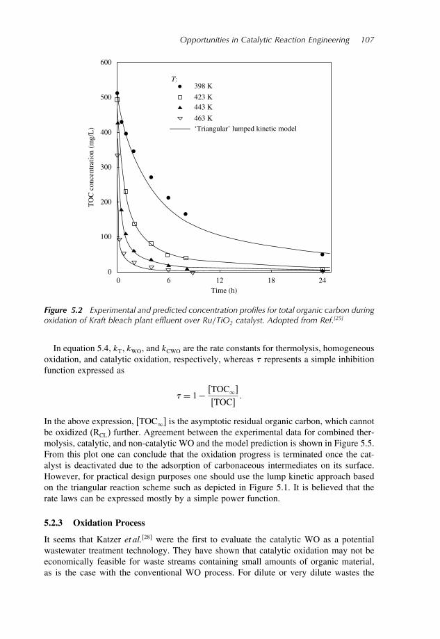
Opportunities in Catalytic Reaction Engineering 107
600
T:398 K
423 K443 K
463 K
500
400
300
200
100
00 6
Time (h)12 18 24
‘Triangular’ lumped kinetic model
TO
C c
once
ntra
tion
(mg/
L)
Figure 5.2 Experimental and predicted concentration profiles for total organic carbon duringoxidation of Kraft bleach plant effluent over Ru/TiO2 catalyst. Adopted from Ref.[25]
In equation 5.4, kT kWO, and kCWO are the rate constants for thermolysis, homogeneousoxidation, and catalytic oxidation, respectively, whereas represents a simple inhibitionfunction expressed as
= 1− TOCTOC
In the above expression, TOC is the asymptotic residual organic carbon, which cannotbe oxidized (RCL) further. Agreement between the experimental data for combined ther-molysis, catalytic, and non-catalytic WO and the model prediction is shown in Figure 5.5.From this plot one can conclude that the oxidation progress is terminated once the cat-alyst is deactivated due to the adsorption of carbonaceous intermediates on its surface.However, for practical design purposes one should use the lump kinetic approach basedon the triangular reaction scheme such as depicted in Figure 5.1. It is believed that therate laws can be expressed mostly by a simple power function.
5.2.3 Oxidation Process
It seems that Katzer et al.28 were the first to evaluate the catalytic WO as a potentialwastewater treatment technology. They have shown that catalytic oxidation may not beeconomically feasible for waste streams containing small amounts of organic material,as is the case with the conventional WO process. For dilute or very dilute wastes the

108 Chemical Engineering
Cac
etic
aci
d (m
mol
/ L)
Cac
etic
aci
d (m
mol
/ L)
Time (h)Time (h)
8
6
4
2
00 6 12 18 24
T: Exp.398 K423 K443 K463 K
‘Triangular’ lumpedkinetic model
Figure 5.3 Experimental and predicted concentration profiles for acetic acid during oxida-tion of Kraft bleach plant effluent over Ru/TiO2 catalyst. Adopted from Ref.[25]
kCWO
kf
kT
kWOTOC
RCL
CG
CS
Figure 5.4 Inhibition–deactivation reaction scheme proposed by Belkacemi et al.[27]
adiabatic temperature rise is too small, therefore additional fuel is needed. To achieveeconomic throughputs and conversions, the oxidation has to be carried out autothermally,which requires preheating of the feed stream by the stream leaving the oxidation reactor.Because energy costs preclude vaporization, wet reactors must operate at pressures above

Opportunities in Catalytic Reaction Engineering 109
20
TOC
CG
CS
Time (min)
TO
C, C
G a
nd C
S (1
03 mg/
L) 15
10
5
00 10 20 30 40 50 60
Figure 5.5 Experimental and predicted concentration profiles for combined thermolysis,catalytic, and non-catalytic wet oxidation of high-strength alcohol distillery liquor overMnO2/CeO2 catalyst. Adopted from Ref.[27]
the vapor pressure of water. Equipment to achieve intimate contacting of the three phaseshas been predominantly in the form of slurry or fixed bed reactors in which the two fluidphases flow through a stationary bed of catalyst concurrently upwards (bubble-columnfixed bed) or downwards (trickle bed). Trickle bed reactors avoid the disadvantages ofseparating small catalyst particles from the liquid stream associated with slurry reactorsand also avoid the limitation of flow rates encountered with up-flow through fixed beds.A reactor with a high liquid to catalyst ratio (e.g. slurry reactor) should not be used forwastewaters containing pollutants that tend to polymerize13. A block diagram of theprocess employing a trickle bed reactor is shown in Figure 5.6.Several catalytic WO processes were commercialized in the mid-1980s in Japan. They
are all based on heterogeneous catalysts containing precious metals deposited on titaniaor titania–zirconia carriers. In comparison to conventional WO units, some of theseprocesses are able to oxidize recalcitrant acetic acid and ammonia. Wastewater treatedin these units can either be discharged directly into an open body of water or reusedas process water. The catalytic wet oxidation system (NS-LC) of Nippon-Shokubai, forexample, which operates at temperature of 220C and total pressure of 40 bars, is capableof achieving a 99% reduction of TOC at a liquid-hourly-space velocity (LHSV) of 2. Itemploys a Pt–Pd/TiO2–ZrO2 catalyst in the form of honeycomb or particles. For highCOD value wastewaters, it consists of a shell-and-tube reactor with catalyst-filled tubes.The Osaka Gas catalytic process uses a catalyst composed of a mixture of precious andbase metals on titania or titania–zirconia carriers (honeycomb or spheres). The catalystlifetime is reported to be longer than eight years. It treats efficiently a variety of municipalwaste streams as well as industrial wastewaters.

110 Chemical Engineering
Purified water
Waste water
PumpSeparator
Gas
Trickle bedreactor
Air
Preheater
Heatexchanger
Figure 5.6 Schematic drawing of a CWO process with single-pass trickle bed reactor
When a wastewater contains relatively low concentrations of organic material thedriving force for the chemical oxidation is very low, therefore some kind of a pre-concentration may be needed29. A process which uses activated carbon as an adsorption–pre-concentration step is shown in Figure 5.7 in combination with a trickle bed reactor.
Waste water Recycle Air
Preheater Pump
Separator
Gas
Trickle bedreactor
Adsorber
Purified water
Figure 5.7 Schematic drawing of a CWO process with adsorber for pre-concentration andrecycled trickle bed reactor

Opportunities in Catalytic Reaction Engineering 111
Once the carbon bed is saturated with organics, hot water at temperatures up to 180Cand elevated pressure is recycled through the adsorber where most of the organics aredesorbed, and through the reactor where the organics are subsequently catalyticallydestructed. Polaert et al.30 recently proposed a similar two-step adsorption–desorptionprocess. They used a single bi-functional reactor where activated carbon is first used asan adsorbent and then as a catalyst. These two combined adsorption–oxidation processesoffer good potential for treating diluted wastewaters at moderate flow rates. In theproposed two processes, it is advantageous that eventually leached metal catalysts alsoplay an active catalytic role12 within the close loop and thus they do not pollute theenvironment.It should be emphasized that catalytic WO processes are primarily designed to oxidize
organic pollutants into intermediates more amenable to biological treatment, since thecomplete oxidation may be prohibitively expensive. Therefore the catalytic WO unitsare installed at the very source of water pollution and are usually used as a pre-treatmentfor cheaper classical biological systems.
5.3 Catalytic Denitrification of Drinkable Water
Nitrates and nitrites are ubiquitous groundwater contaminants particular in the areasof extensive agriculture fertilizing. The toxicity of nitrates to humans is due to thebody’s reduction of nitrate to nitrite. The content of nitrates in groundwater that exceedthe maximum admissible concentration (e.g. 50mg/L as set by the European WaterDirective) must be reduced in order to avoid health risk. Therefore the removal of nitratesfrom drinkable water is an emerging technology, which is going to keep busy manyresearchers in the coming years. Kapoor and Viraraghavan31 presented in their state-of-the-art review all treatment methods that are currently available. According to the capitaland operational cost, the ion-exchange technique is the most favorable but disposing thespent brine for regeneration poses a serious problem in non-coastal locations. However,the most promising techniques for nitrate removal without creating secondary waste arebiological digestion and catalytic denitrification by employing noble metal catalysts. Themain reasons for slow transfer of biological digestion into a practice are concerns ofpossible bacterial contamination and presence of residual organics in treated water, whichadditionally increase the chlorine demand. As an alternative to the biological digestion,Vorlop and Tacke32 introduced the reduction of nitrates in drinkable water by hydrogenover a solid catalyst at mild reaction conditions: temperatures between 5C and 25C,and hydrogen partial pressures up to 7 bar. Pintar10 has recently provided a thoroughreview on the catalytic treatment of drinkable water.
5.3.1 Catalysts
In this process, nitrates are selectively reduced via intermediates into nitrogen, there-fore the electro-neutrality of the aqueous solution is sustained by replacing nitrates withhydroxide ions. Supported bimetallic catalysts such as Pd–Cu, Pd–Sn, Pd–In, and Pt–Cuare known to have great potential for the reduction of nitrates. Unfortunately, these cata-lysts are not suppressing sufficiently the side reaction toward the formation of ammonia,which is highly undesirable in water for drinking (below 0.5mg/L). Hörold et al.33 have

112 Chemical Engineering
shown that Pd hydrogenation catalyst doped with Cu is a selective bimetallic catalystfor the transformation of nitrates to nitrogen. At the initial nitrate concentration level of100mg/L they achieved the selectivity of 82 mol%, which can be even further increasedby employing a mixture of supported Pd–Cu and Pd catalysts and lowering the hydro-gen partial pressures. It is believed that the key intermediate product in the process ofcatalytic nitrate reduction is NO34. Pintar and Kajiuchi35 and later Deganello et al.36,who studied the same reaction over various Pd–Cu bimetallic catalysts, reported that thenitrate to nitrite reduction undergoes a structure-insensitive reaction. It was demonstratedthat the reaction selectivity strongly depends on the spatial distribution of Pd and Cumetallic phases; the highest selectivity was obtained with a catalyst sample in whichthe very first sub-layers were enriched by palladium atoms3738. Similar behavior withrespect to the minimum accumulation of nitrite ions was obtained with Pd–Cu bimetalliccatalysts prepared by the sol–gel preparation technique39. A reason for the low reactionselectivity found in some cases (less than 70 mol%) might be the inappropriateness ofthe textural properties of the catalyst surface and due to the ratio of the two metals3336.Besides Pd–Cu bimetallic catalysts, new alumina-supported Pd–Sn and Pd–In catalystshave been used for the efficient treatment of nitrate-polluted drinkable water40. It seems,however, that the latter two types of catalyst prepared by a deposition–precipitatedmethod are more active as well as more selective for nitrate removal. According to Prüsseet al.40 the selectivity may also increase if formic acid is used as a source of hydro-gen. Recently a Pd/SnO2 catalyst
41, palladium–tin catalysts on acrylic resin catalyst42,titania-supported Pd–Cu catalysts43, and palladium- and platinum-based catalysts dopedwith copper, silver, or gold44 were employed successfully. Pd–Cu/Mg/Al–hydrotalcitesbased catalysts have also experienced a good activity/selectivity45. Matatov-Meytalet al.46 used woven cloths made of glass fibers impregnated with Pd and reported aboutthe same activity as found with the conventional powdered catalysts. However, knowl-edge about the selective catalytic reduction of nitrates in drinkable water is still far fromcomplete, therefore more mechanistic studies with different catalytic systems would beappreciated.
5.3.2 Reduction Kinetics
Quantitative rate data on the catalytic reduction of nitrates in drinkable water are rela-tively scarce. One of the first works concerning kinetics is that of Tacke and Vorlop47
who employed a Pd–Cu bimetallic catalyst containing 5wt.% of Pt and 1.25wt.% ofCu in a slurry reactor. Measurements of the initial rates resulted in a power-law rateexpression. They reported a power of 0.7 with respect to the nitrate concentration, and anindependency on the hydrogen partial pressure providing this pressure exceeded 1 bar.Pintar et al.48 reported a complete kinetic model of the Langmuir–Hinshelwood typewritten in the form
−rNO−3=−dCNO−
3
dt= kappKNO−
3K
1/2H2
CNO−3p1/2H2
1+KNO−3CNO−
31+K
1/2H2
p1/2H2
(5.6)
which accounts for both the non-competitive equilibrium nitrate and the dissociativehydrogen adsorption steps. Here the irreversible bimolecular reaction between adsorbednitrate ion and hydrogen is considered as the rate-limiting step. In slurry reactor, the
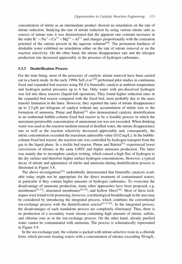
Opportunities in Catalytic Reaction Engineering 113
concentration of nitrite as an intermediate product showed no retardation on the rate ofnitrate reduction. Studying the rate of nitrate reduction by using various nitrate salts assources of nitrate ions it was demonstrated that the apparent rate constant increases inthe order K+<Na+<Ca2+<Mg2+<Al3+ and changes proportionally with the ionizationpotential of the cations present in the aqueous solution49. The permanent hardness ofdrinkable water exhibited no retardation either on the rate of nitrate removal or on thereaction selectivity. On the other hand, the nitrate disappearance rate and the nitrogenproduction rate decreased appreciably in the presence of hydrogen carbonates.
5.3.3 Denitrification Process
For the time being, most of the processes of catalytic nitrate removal have been carriedout in a batch mode. In the early 1990s Sell et al.50 performed pilot studies in continuousfixed and expanded bed reactors using Pd–Cu bimetallic catalyst at ambient temperatureand hydrogen partial pressures up to 6 bar. Only water with pre-dissolved hydrogenwas fed into these reactors (liquid-full operation). They found higher reduction rates inthe expanded bed reactor compared with the fixed bed, most probably due to the masstransfer limitation in the latter. However, they reported the rates of nitrate disappearanceup to 2.5 g/h per kilogram of catalyst without any accumulation of nitrite ions or theformation of ammonia. Pintar and Batista51 also demonstrated catalytic denitrificationin an isothermal bubble-column fixed bed reactor to be a feasible process in which themaximum permissible concentration of ammonium ion was not exceeded. When drinkingwater was used as the reaction medium instead of distilled water, the nitrate disappearancerate as well as the reaction selectivity decreased appreciably and, consequently, thenitrite concentration exceeded the maximum admissible value (0.02mg/L). In the bubble-column fixed bed reactor, the reaction rate was controlled by hydrogen transport from thegas to the liquid phase. In a trickle bed reactor, Pintar and Batista51 experienced lowerconversions of nitrates at the same LHSV and higher ammonia production. The latterwas mainly due to incomplete catalyst wetting, which caused a high flux of hydrogen tothe dry surface and therefore higher surface hydrogen concentrations. However, a typicaldecay of nitrate and appearance of nitrite and ammonia during denitrification process isillustrated in Figure 5.8.The above investigations51 undoubtedly demonstrated that bimetallic catalysts avail-
able today might not be appropriate for the direct treatment of contaminated waters,in particular if they contain higher amounts of hydrogen carbonates. To overcome thedisadvantage of ammonia production, many other approaches have been proposed, e.g.membranes5253, structured membranes5455, and hollow fibers56. Most of these tech-niques were found to be promising; however, a technological breakthrough in the area maybe considered by introducing the integrated process, which combines the conventionalion-exchange process with the denitrification reactor515758. In the integrated process,the disadvantages of each standalone process are completely eliminated. Thus, there isno production of a secondary waste stream containing high amounts of nitrate, sulfate,and chlorine ions as in the ion-exchange process. On the other hand, already purifiedwater cannot be contaminated with ammonia. The process is schematically representedin Figure 5.9.In the ion-exchange part, the column is packed with nitrate-selective resin in a chloride
form, which prevents treating waters with a concentration of nitrates exceeding 50mg/L.

114 Chemical Engineering
100
80
60
Cni
trat
e (m
g/L
)
Time (min)
Cni
trite
: Cam
mon
ia (
mg/
L)
40
20
00 100 200 300 400 500 600
0
5
10
15
20
25
p(H2): 0.11 bar
pH: 5.5 (const.)
T : 298 Kp(H2): 0.53 bar
Ptot: 1.0 bar
mcat: 3.0 g: dp: 1.7 mm
CNO3,φ: 100.0 mg/L–
Figure 5.8 Typical concentration profiles for nitrate, nitrite, and ammonia (© and ) duringhydrogenation of a model drinking water at two different hydrogen pressures over a bimetallicPd(1%)–Cu(0.3%)/Al2O3 catalyst
Blendedproduct water
Byp
ass
raw
wat
er
Raw waterPump
EqualizationtankNaCl
solution
PC
CatalyticreactorH2
orH2–N2
N2
H2
pH HCl
Pump
Ion-exchangecolumn
Figure 5.9 Schematic drawing of a combined ion exchange–catalytic denitrification process
Depending on the field capacity, contaminated level, and water demands the nitrate-freeeffluent from the ion-exchange column can be arbitrarily blended with the bypassednon-treated groundwater in order to meet the water quality requirements. The spent resinis regenerated in close circuit with sodium chloride solution, the concentration of which

Opportunities in Catalytic Reaction Engineering 115
can be approximately an order of magnitude lower compared with the conventionalion-exchange regeneration process. The regenerant solution containing high amounts ofnitrates circulates through the fixed bed reactor packed with a proprietary Pd–Cu/Al2O3
bimetallic catalyst where nitrates are reduced by hydrogen. Nitrite and ammonia formedin the reactor cannot be transported into the ion-exchange-treated effluent and thereforedo not affect the water quality. The fixed bed reactor operates at ambient temperature andpressure. The pH of the liquid phase is controlled and kept at a value of 5 simply by addingHCl to the NaCl solution. The regenerant continues recycling through the ion-exchangecolumn and the reactor until the resin reaches sufficient chloride loading. The integratedprocess is capable of destroying about 95% of waste brine, which is a tremendousimprovement over the conventional ion-exchange process. Accumulation of sulfate ionsin the closed circuit was found harmless to the nitrate capacity of the chloride-type resin.The use of HCl for pH control is also advantageous because there is no need for theregenerant makeup with NaCl. Namely, the stoichiometrically required amount of chlorideions for the subsequent regeneration cycle is provided by the neutralization of hydroxideions produced in the nitrate reduction step. In a continuous and efficiently designedoperation, one fixed bed denitrification reactor may serve at least three ion-exchangecolumns.
5.4 Preferential CO Oxidation
Selective oxidation of carbon monoxide in excess of the hydrogen or PROX process hasbecome a renewed interest for many researchers due to its potential of making hydro-gen acceptable for low-temperature PEMFC. In order to avoid problems associated withhydrogen storage (in automotive application in particular), hydrogen should be producedby the autothermal reforming of hydrocarbon fuels at a place of utilization. Indeed, thecatalytic decomposition of ammonia appears to be another appealing process for CO-freehydrogen fuel. However, the composition of gas leaving the reformer and water gas-shift(WGS) reactor does not fit the requirements for PEMFC application. Typically, it con-tains 45–75 vol% of H2, 15–25 vol% of CO2, a few vol% of H2O, traces of unconvertedfuel, and 0.5–2 vol% of CO. CO is a catalyst poison for the Pt gas diffusion anodeof PEMFC, which can only tolerate CO in concentrations below 50 ppm59, in somecases even below 10 ppm60. In order to reduce the CO concentration in reformate,several approaches are currently under investigation: preferential oxidation (PROX), cat-alytic methanation, and Pd-membrane separation. Among these, PROX offers the lowestcost process for reducing CO content to the desired level without excessive hydrogenconsumption.
5.4.1 Catalysts
A PROX catalyst needs to be active and selective; it should oxidize CO without oxidizinga large amount of hydrogen. It should prevent side reactions such as reverse WGS andmethanation and be capable of operating under high steam and CO2 content. Oxidationof hydrogen reduces the overall fuel efficiency on one side, but depending on thecatalyst nature it may also affect the catalyst activity via produced water. The lowerthe catalyst activity, the higher is the O2/CO ratio that has to be used in order to

116 Chemical Engineering
completely oxidize CO to CO2. Catalysts employed in PROX reactors mostly involvehigh platinum group metals (PGM) loading on high surface area supports and are operatedin a temperature range of 80–200C. Catalyst formulation comprises Pt or promotedPt, Ru, Pd, alloys of Pt–Sn or Pt–Ru, or Rh on alumina or on molecular sieves61 ormore recently, Au catalysts62. Among these, Pt catalysts have been the most studiedand appear to offer the best activity and selectivity over a wide range of temperatures.Copper catalysts on alternative supports such as ceria, ceria-samaria, or other ceria-promoted supports have also been developed in an attempt to provide selective surfaceoxygen for CO oxidation at low temperatures6364. Ghenciu59, Shore and Farrauto60,and Choudhary and Goodman65 have recently provided a review on fuel processingcatalysts for hydrogen production for PEMFC technology.Oh and Sinkevitch66 compared the efficiency of several PGM loading (0.5%) catalysts
for the PROX reaction and found that the CO conversion decreases in the following order:Ru/Al2O3 > Rh/Al2O3 > Pt/Al2O3 > Pd/Al2O3. Although the Pd catalyst exhibiteda similar activity as Ru and Rh catalysts at low temperatures, its activity at highertemperatures was found to be significantly poorer. The authors attributed this effect tothe change in oxidation state of Pd with increasing reaction temperature. Despite Ru andRh catalysts demonstrating high efficiency, these catalysts have not been explored in fulldetail. Nevertheless, there are two drawbacks of a ruthenium catalyst: first, its operatingtemperature is 140–200C, thus well above the operating temperature of PEMFC, andsecond, it also acts as a methanation catalyst60.Gold-based catalysts have been investigated with a great interest although metal gold is
known to be inefficient in CO oxidation. On the other hand, supported nano-gold clustersare found highly active and therefore promising in the PROX process. For example, onmanganese oxide-supported gold catalyst, over 95% conversions of CO were reportedin a temperature range of 50–80C, which fits the operating temperature of PEMFC67.In spite of the fact that supported gold catalysts are almost insensitive to CO2 and thattheir activity even enhances with moisture, Pt catalysts have an advantage over Aucatalysts since the latter undergo relatively fast deactivation induced by oxygen65. Thestability of nano-Au catalyst can be substantially increased by a temperature-programmedreduction–oxidation treatment of an Au–phosphine complex on TiO2
68. It is also worthmentioning here that a bimetallic carbon-supported PtSn system shows some superiorityover Pt/Al2O3 catalyst
69.Recently mixed oxides of Cu and Ce have been reported as very promising catalysts
for PROX. In a comparative study of Pt/–Al2O3, Au/–Fe2O3, and CuO–CeO2 cata-lysts for the selective oxidation of CO in excess of hydrogen, Avgouropoulos et al. 70
have undoubtedly demonstrated that the Au catalyst is the most active at low tem-perature, while the selectivity of CuO–CeO2 is remarkably higher than that of bothAu and Pt systems. Platinum on alumina was found to be the most resistant to waterand CO2. At temperatures between 45C and 90C, an inexpensive nano-structuredCu01Ce09O2−y catalyst (prepared by a sol–gel technique) was found provide 100% selec-tivity with CO conversions up to about 60% as depicted in Figure 5.1064. At highertemperatures much higher conversions can be attained but at the expense of selectiv-ity. Kandoi et al.71 have recently provided a theoretical basis for why the catalystsbased on Au and Cu are superior to Pt-based catalyst for the oxidation of trace COin reformate gases at low temperatures, i.e. close to the operational temperature ofPEMFC.

Opportunities in Catalytic Reaction Engineering 117
100
80
60
40
20
040 60 80 100 120 140 160
Sele
ctiv
ity (
%)
100
80
60
40
20
040 60 80 100
Temperature (°C)
120 140 160
CO
con
vers
ion
(%)
Figure 5.10 Selectivity and CO conversion as a function of temperature obtained overnanostructured copper-cerium oxide at different values of (full and empty symbols) andhydrogen concentration in the reactor feed ( and no hydrogen in feed)
5.4.2 PROX Kinetics
Initial conclusions on the kinetics of selective oxidation of CO in hydrogen reach gaswere drawn from what is known about CO oxidation (in the absence of H2) on single-crystalline and supported PGM catalysts. Namely, some early investigations under ultra-high vacuum conditions72 and more recently in high pressure region73 have found twodistinct reaction regimes: (i) high rate regime, which occurs at high temperatures onthe surface covered with very small amounts of adsorbed CO, and (ii) low rate regime,which takes place at low temperatures on the catalyst surface predominantly covered withadsorbed CO. Both regimes were modeled by the Langmuir–Hinshelwood mechanism,which is associated with the reaction order approaching −1 with respect to the CO partialpressure and close to +1 for the oxygen partial pressure for the low rate regime, and+1 for both the components in the high rate regime. Assuming the addition of hydrogen

118 Chemical Engineering
does not change the oxidation mechanism, one would expect that the reaction takes placein the low rate regime since the low temperature operation of PROX (below 250C, and≤ 2= 2pO2
/pCO is dictated by PEMFC. Kahlich et al.74 have published an extensivekinetic study of the selective oxidation of CO in hydrogen reach gas on Pt/Al2O3. Ina wide range of CO partial pressures and temperatures between 150C and 250C, andthe process parameter values relevant to PROX, they have shown that the oxidationrate can be well represented by the power-law kinetics: the order of −04 with respectto the CO partial pressure and order of +08 with respect to the oxygen partial pressure.The reaction orders and the activation energy of 71 kJ/mol was found consistent with thereaction occurring on the surface predominantly covered by adsorbed CO, which blocksthe oxygen adsorption. An interesting kinetics is found in the work of Han et al.75 whooxidized CO in a methanol reformate over a Ru/–Al2O3 catalyst. In a temperaturerange of 80–120C, these authors proposed the power-law kinetics with the temperature-dependent orders between −029 and −066 for carbon monoxide and +030 and +080for oxygen, respectively, whereas the activation energy was reported to be 48 kJ/mol.Oxidation kinetics on transition metal mixed oxide catalysts was also first interpreted
by means of the Langmuir–Hinshelwood mechanism and in terms of a synergistic effectresulting from the interaction of different materials76. The rate equation in the followingform was proposed:
rCO = kLKLPCOPmO2
1+KLPCO
(5.7)
where the parameters kL and KL represent the surface reaction rate and CO adsorptionequilibrium constants, respectively, and P = partial pressure. Both parameters are wellcorrelated by the Arrhenius law. The reaction order with respect to oxygen was reportedto be a very small number, close to 0, whereas the activation energy was found in a rangeof 73–94 kJ/mol. Sedmak et al.64 modeled the kinetics of selective CO oxidation overthe CuxCe1−xO2−y nanostructured catalysts by means of the Mars–van Krevelen type ofkinetics, which is based on a redox mechanism, thus
rCO = kCOkO2PCOP
nO2
05kCOPCO+kO2PnO2
(5.8)
The parameters kCO and kO2are taken to be the reaction rate constants for the reduction of
surface by CO and the surface re-oxidation by O2, respectively, and are subjected to theArrhenius law. The order with respect to oxygen n takes a value of 0.2. It is interestingto note that the experimental data of Sedmak et al.64 can also be well correlated byequation 5.7 with m= 015. However, the transient experiments with a step change of COconcentration in the reactor feed have revealed the involvement of lattice oxygen even atlow temperatures, thus confirming the appropriateness of using the Mars–van Krevelenkinetic formulation7778. Figure 5.11 shows a comparison between the experimentalresponses and the predictions made by a fixed bed reactor model accounting for the ratelaw given by equation 5.8.
5.4.3 PROX Process
From a process point of view (reformer→WGS reactor→PROX reactor→fuel cell) thePROX reactor should be advantageously operated between the outlet temperature of

Opportunities in Catalytic Reaction Engineering 119
2.0
1.5
1.0
0.5
0.00 50 100 150 200
CO
con
cent
ratio
n (v
ol%
)
He → 0.5 vol% CO/He; HTOT = 0.25
He → 1 vol% CO/He; HTOT = 0.35
He → 2 vol% CO/He; HTOT = 0.35
Model
1.2
0.9
0.6
0.3
0.00 50 100
Time (S)
150 200
CO
2 co
ncen
trat
ion
(vol
%)
Figure 5.11 Experimental and predicted responses in CO and CO2 concentrations in thereactor outlet stream after step change in the reactor feed stream from helium to a differentCO concentration on fully oxidized copper-cerium oxide
the WGS reactor and the inlet temperature of fuel cell ∼80C. The process must beprimarily designed for highly selective oxidation of CO since any loss of hydrogen, theprimary electrochemical fuel, reduces the competitiveness and efficiency of the process.Bearing in mind that the process is installed as the very last stage of the hydrogen

120 Chemical Engineering
production line, it must provide hydrogen fuel over a wide range of PEMFC outputconditions (turndown ratios). Therefore the PROX catalyst must also be able to operateefficiently in a wide range of space velocities, under severe transient conditions. Itmust handle the CO content (e.g. 10 ppm) at high as well as at low throughputs. It isknown, for example, that at very low space velocities, a Pt-based catalyst may produceCO by the reverse WGS reaction. The inlet temperature has to be compatible withthe outlet temperature of the upstream WGS unit, and because the oxidation of COand H2 is a highly exothermic reaction, the PROX exit stream must be cooled downto the operating temperature of PEMFC (about 80C). Efficient cooling and minimalpressure drop within the reactor in particular dictate the catalyst shape design, whichseems to be advantageously in the form of washcoat monoliths. In order to achieve highthermal efficiency, a fuel processor should consist of steam reformer, CO shift converter,PROX reactor, steam generator, burner, and heat exchanger in one package78. Since thetemperature control in the secondary hydrogen cleaning system is crucial, it should beadvantageous to employ microstructured reactors, which are known for their feasibility ofdynamic operation7980. Some design considerations of the PROX process and catalystsare briefly discussed in a recent article by Shore and Farrauto60.
5.5 Conclusions
The common key issue in all three examples is a catalyst. While a catalyst for WO doesnot need to be selective, denitrification of drinkable water and preferential oxidation ofCO call for a very selective catalyst.Catalytic WO can be considered nowadays as a mature technology. Nevertheless, due
to the variety of wastewater that has to be treated, one type of catalyst cannot fulfill allthe needs. Therefore the catalyst must be tailored for each particular application and madeof inexpensive materials. In order to reduce leaching, the catalytically active compoundshave to be incorporated into a lattice of catalyst support. It would be advantageous todesign a catalyst for treatment in single-pass reactors that had a minimum lifetime ofover 500 h.Removal of nitrate from drinkable water is still far from maturity. A direct treatment or
single-pass process even with a very selective catalyst is not likely to be feasible becausedrinkable water should not be in contact with a noble metal catalyst. At this moment onecan consider the combined ion exchange and denitrification process to be advantageousover the conventional ion-exchange technology, the main drawback of which is a harmfuldisposing of large amounts of spent brine. In the combined process, a Pd–Cu bimetalliccatalyst seems to be efficient enough but more work in a pilot scheme would positivelyhelp to push the technology forward.While more CO-tolerant fuel cells are being developed, efforts in developing more
selective catalysts to remove higher amounts of CO (0.5–1.0%) from the hydrogen-reachreformate prior to entering the cell are continuing. These efforts are accompanied bycost reduction. Monolithic types of catalysts, especially those containing Pt, have alreadybeen successfully demonstrated in the PROX process. Nevertheless, some other inex-pensive catalytic systems, e.g. copper-cerium, also remain attractive for low-temperatureoperation.

Opportunities in Catalytic Reaction Engineering 121
References
[1] Kochloefl K. 2001. Development of industrial solid catalyst, Chem. Eng. Technol., 24,229–234.
[2] Sadana A. and Katzer J.R. 1974. Catalytic oxidation of phenol in aqueous solutions overcopper oxide, Ind. Eng. Chem. Fundam., 13, 127–134.
[3] Baldi G., Goto S., Chow C.K. and Smith J.M. 1974. Catalytic oxidation of formic acid inwater, Ind. Eng. Chem. Proc. Des. Dev., 13, 447–452.
[4] Levec J. and Smith J.M. 1976. Oxidation of acetic acid solutions in a trickle-bed reactor,AIChE J., 22, 159–168.
[5] Mishra V.S., Mahajani V.V. and Joshi J.B. 1995. Wet air oxidation, Ind. Eng. Chem. Res.,34, 2–48.
[6] Levec J. and Pintar A. 1995. Catalytic oxidation of aqueous solutions of organics. Analternative method for removal of toxic pollutants from wastewaters, Catal. Today, 24, 51–58.
[7] Matatov-Meytal Y.I. and Sheintuch M. 1998. Catalytic abatement of water pollutants, Ind.Eng. Chem. Res., 37, 309–326.
[8] Luck F. 1999. Wet air oxidation: past, present and future, Catal. Today, 53, 81–91.[9] Imamura S. 1999. Catalytic and noncatalytic wet oxidation, Ind. Eng. Chem. Res., 38,
1743–1753.[10] Pintar A. 2003. Catalytic processes for the purification of drinking water and industrial
effluents, Catal. Today, 77, 451–465.[11] Mantzavinos D., Hellenbrand R., Livingston A.G. and Metcalfe I.S. 1996. Catalytic oxidation
of p-coumaric acid: partial oxidation intermediates, reaction pathways and catalyst leaching,Appl. Catal. B, 7, 379–396.
[12] Fortuny A., Font J. and Fabregat A. 1998. Wet air oxidation of phenol using active carbonas catalyst, Appl. Catal. B, 19, 165–173.
[13] Pintar A. and Levec J. 1992. Catalytic oxidation of organics in aqueous solutions. I. Kineticsof phenol oxidation, J. Catal., 135, 345–357.
[14] Imamura S., Fukuda I. and Ushida S. 1988. Wet oxidation catalyzed by ruthenium supportedon cerium oxides, Ind. Eng. Chem. Res., 27, 718–721.
[15] Gallezot P., Chaumet S., Perrard A. and Isnard P. 1997. Catalytic wet air oxidation of aceticacid on carbon-supported ruthenium catalysts, J. Catal., 168, 104–109.
[16] Barbier Jr J., Delanoë F., Jabouille F., Blanchard G. and Duprez D. 1998. Total oxidation ofacetic acid in aqueous solutions over noble metal catalysts, J. Catal., 177, 378–385.
[17] Béziat J.-C., Besson M., Gallezot P. and Durecu S. 1999. Catalytic wet air oxidation ofcarboxylic acids on TiO2 supported ruthenium catalysts, J. Catal., 182, 129–135.
[18] Pintar A., Besson M. and Gallezot P. 2001. Catalytic wet air oxidation of Kraft bleachingplant effluents in the presence of titania and zirconia supported ruthenium, Appl. Catal. B,30, 123–139.
[19] Cybulski A. and Trawczynski J. 2004. Catalytic wet air oxidation of phenol over platinumand ruthenium catalyst, Appl. Catal. B, 47, 1–13.
[20] Pintar A. and Levec J. 1992. Catalytic liquid-phase oxidation of refractory organics in wastewater, Chem. Eng. Sci., 47, 2395–2400.
[21] Pintar A. and Levec J. 1994. Catalytic liquid-phase oxidation of phenol aqueous solutions.A kinetic investigation, Ind. Eng. Chem. Res., 33, 3070–3077.
[22] Eftaxias A., Font J., Fortuny A., Giralt J., Fabregat A. and Stüber F. 2001. Kinetic modelingof catalytic wet air oxidation of phenol by simulated anneling, Appl. Catal. B, 33, 175–190.
[23] Hamoudi S., Belkacemi K. and Larachi F. 1999. Catalytic oxidation of aqueous phenolicsolutions catalyst deactivation and kinetics, Chem. Eng. Sci., 54, 3569–3576.
[24] Li L., Chen P. and Gloyna E.F. 1991. Generalized kinetic model for wet oxidation of organiccompounds, AIChE J., 37, 1687–1697.

122 Chemical Engineering
[25] Pintar A., Bercic G., Besson M. and Gallezot P. 2004. Catalytic wet-air oxidation of industrialeffluents: total mineralization of organics and lumped kinetic modelling, Appl. Catal. B, 47,143–152.
[26] Donlagic J. and Levec J. 1999. Wet oxidation of an azo dye: lumped kinetics in batch andmixed flow reactors, AIChE J., 45, 2571–2579.
[27] Belkacemi K., Larachi F., Hamoudi S., Tucotte G. and Sayari A. 1999. Inhibition anddeactivation effects in catalytic wet oxidation of high-strength alcohol – distillery liquors,Ind. Eng. Chem. Res., 38, 2268–2274.
[28] Katzer J.R., Ficke H.H. and Sadana A. 1976. An evaluation of aqueous phase catalyticoxidation, J. Water Poll. Control Fed., 48, 920–933.
[29] Levec J. and Pintar A. 1997. Process for treating industrial waste waters with low concentra-tions of toxic pollutants. EP 0 664 771 B1, European Patent Office, Muenchen, 29 January1997.
[30] Polaert I., Wilhelm A.M. and Delmas H. 1997. Phenol wastewater treatment by a two-stepadsorption-oxidation process on activated carbon, Chem. Eng. Sci., 57, 1585–1590.
[31] Kapoor A. and Viraraghavan T. 1997. Nitrate removal from drinking water – Review, J.Environ. Eng., 123, 371–380.
[32] Vorlop K.-D. and Tacke T. 1989. First steps towards noble-metal catalyzed removal of nitrateand nitrite from drinking water, Chem. Ing. Tech., 64, 836–837.
[33] Hörold S., Vorlop K.-D., Tacke T. and Sell M. 1993. Development of catalysts for a selectivenitrate and nitrite removal from drinking water, Catal. Today, 17, 21–30.
[34] Wärnå J., Turunen I., Salmi T. and Maunula T. 1994. Kinetics of nitrate reduction in monolithreactor, Chem. Eng. Sci., 49, 5763–5773.
[35] Pintar A. and Kajiuchi T. 1995. Catalytic liquid-phase hydrogenation of aqueous nitratesolutions, Acta Chim. Slovenica, 42, 431–449.
[36] Deganello F., Liotta L.F., Macaluso A., Venezia A.M. and Deganello G. 2000. Catalyticreduction of nitrates and nitrites in water solution on pumice-supported Pd–Cu catalysts,Appl. Catal. B, 24, 265–273.
[37] Batista J., Pintar A. and Ceh M. 1997. Characterization of supported Pd–Cu catalysts bySEM, EDXS, AES and catalytic selectivity measurements, Catal. Lett., 43, 79–84.
[38] Pintar A., Batista J., Arcon I. and Kodre A. 1998. Characterization of gamma-Al2O3 supportedPd–Cu bimetallic catalysts by EXAFS, AES and kinetic measurements, Stud. Sufr. Sci.Catal., 118, 127–136.
[39] Strukul G., Pinna F., Marella M., Meregalli L. and Tomaselli M. 1996. Sol–gel palladiumcatalysts for nitrate and nitrite removal from drinking water, Catal. Today, 27, 209–214.
[40] Prüsse U., Hähnlein M., Daum J. and Vorlop K.-D. 2000. Improving the catalytic nitratereduction, Catal. Today, 55, 79–90.
[41] Gavagnin R., Biasetto L., Pinna F. and Strukul G. 2002. Nitrate removal in drinking waters:the effect of tin oxides in the catalytic hydrogenation of nitrate by Pd/SnO2 catalysts, Appl.Catal. B, 38, 91–99.
[42] Roveda A., Benedetti A., Pinna F. and Strukul G. 2003. Palladium-tin catalysts on acrylicresins for the selective hydrogenation of nitrate, Inorg. Chim. Acta, 349, 203–208.
[43] Gao W., Guan N., Chen J., Guan X., Jin R., Zeng H., Liu Z. and Zhang F. 2003. Titaniasupported Pd–Cu bimetallic catalyst for the reduction of nitrate in drinking water, Appl.Catal. B, 46, 341–351.
[44] Epron F., Gauthard F. and Barbier J. 2002. Influence of oxidizing and reducing treatmentson the metal–metal interactions and on the activity for nitrate reduction of a Pt–Cu bimetalliccatalyst, Appl. Catal. A, 237, 253–261.
[45] Palomares A.P., Prato J.G., Márquez F. and Corma A. 2003. Denitrification of natural wateron supported Pd/Cu catalysts, Appl. Catal. B, 41, 3–13.
[46] Matatov-Meytal Y., Barelko V., Yuranov I. and Sheintuch M. 2000. Cloth catalysts in waterdenitrification: I. Pd on glass fibers, Appl. Catal. B, 27, 127–135.

Opportunities in Catalytic Reaction Engineering 123
[47] Tacke T. and Vorlop K.-D. 1993. Kinetic characterization of catalysts for selective removalof nitrate and nitrite from water, Chem. Ing. Tech., 65, 1500–1502.
[48] Pintar A., Batista J., Levec J. and Kajiuchi T. 1996. Kinetics of the catalytic liquid-phasehydrogenation of aqueous nitrate solutions, Appl. Catal. B, 11, 81–98.
[49] Pintar A., Šetinc M. and Levec J. 1998. Hardness and salt effects on catalytic hydrogenationof aqueous nitrate solutions, J. Catal., 174, 72–87.
[50] Sell M., Bischoff M. and Bonse D. 1992. Catalytic nitrate reduction in drinking water. Resultsand experiences from pilot plant trials, Vom Wasser, 79, 129–144.
[51] Pintar A. and Batista J. 1999. Catalytic hydrogenation of aqueous nitrate solutions in fixed-bed reactors, Catal. Today, 53, 35–50.
[52] Lüdtke K., Peinemann K.-V., Kasche V. and Behling R.-D. 1998. Nitrate removal of drinkingwater by means of catalytically active membranes, J. Membr. Sci., 151, 3–11.
[53] Ilinich O.M., Gribov E.N. and Simonov P.A. 2003. Water denitrification over catalyticmembranes: hydrogen spillover and catalytic activity of macroporous membranes loadedwith Pd and Cu, Catal. Today, 82, 49–56.
[54] Daub K., Emig G., Chollier M.-J., Callant M. and Dittmeyer R. 1999. Studies on the useof catalytic membranes for reduction of nitrate in drinking water, Chem. Eng. Sci., 54,1577–1582.
[55] Centi G., Dittmeyer R., Perathoner S. and Reif M. 1999. Tubular inorganic catalytic mem-brane reactors: advantages and performance in multiphase hydrogenation reactions, Catal.Today, 79, 139–149.
[56] Hähnlein M., Prüsse U., Daum J., Morawsky V., Kröger M., Schröder M., Schnabel M. andVorlop K.-D. 1998. Preparation of microscopic catalysts and colloids for catalytic nitrate andnitrite reduction and their use in hallow fibre dialiser loop reactor, Stud. Surf. Sci. Catal.,118, 99–107.
[57] Pintar A., Batista J. and Levec J. 2001. Catalytic denitrification: direct and indirect removalof nitrates from potable water, Catal. Today, 66, 503–510.
[58] Pintar A., Batista J. and Levec J. 2001. Integrated ion exchange/catalytic process for efficientremoval of nitrates from drinking water, Chem. Eng. Sci., 56, 1551–1559.
[59] Ghenciu A.F. 2002. Review of fuel processing catalysts for hydrogen production in PEMfuel cell systems. Curr. Opin. Solid State Mat. Sci., 6, 389–399.
[60] Shore L. and Farrauto R.J. 2003. PROX catalysts. In, Handbook of Fuel Cells – Fundamentals,Technology and Applications, Vielstich W., Lamm A. and Gasteiger A. (Eds.), Vol. 3, Wiley,Chichester, pp. 211–218.
[61] Igarashi H., Uchida H., Suzuki M., Sasaki Y. and Watanabe M. 1997. Removal of carbonmonoxide from hydrogen-rich fuels by selective oxidation over platinum catalyst supportedon zeolite, Appl. Catal. A, 159, 159–169.
[62] Haruta M., Tsubota S., Kobayashi T., Kageyama H., Genet M.J. and Delmon B. 1993. Low-temperature oxidation of CO over gold supported on TiO2, -Fe2O3 and Co3O4, J. Catal.,144, 175–192.
[63] Avgouropoulos G., Ioannides T., Matralis H.K., Batista J. and Hocevar S. 2001. CuO–CeO2
mixed oxide catalysts for the selective oxidation of carbon monoxide in excess hydrogen,Catal. Lett., 73, 33–40.
[64] Sedmak G., Hocevar S. and Levec J. 2003. Kinetics of selective CO oxidation in excess ofH2 over the nanostructured Cu01Ce09O2−y catalyst, J. Catal., 213, 135–150.
[65] Choudhary T.V. and Goodman D.W. 2002. CO-free fuel processing for fuel cell application,Catal. Today, 77, 65–78.
[66] Oh S.H. and Sinkevitch R.M. 1993. Carbon monoxide removal from hydrogen-rich fuel cellfeedstreams by selective catalytic oxidation, J. Catal., 142, 254–262.
[67] Sanchez R.M.T., Ueda A., Tanaka K. and Haruta M. 1997. Selective oxidation of CO inhydrogen over gold supported on manganese oxides, J. Catal., 168, 125–127.
124 Chemical Engineering
[68] Choudhary T.V., Sivadinarayana C., Chusuei C.C., Datye A.K., Fackler Jr J.P. andGoodman D.W. 2002. CO oxidation on supported nano-Au catalysts synthesized from aAu6PPh3BF42 complex, J. Catal., 207, 247–255.
[69] Schubert M.M., Kahlich M.J., Feldmeyer G., Huttner M., Hackenberg S., Gasteiger H.A. andBehm R.J. 2001. Bimetallic PtSn catalyst for selective CO oxidation in H2-rich gases at lowtemperatures, Phys. Chem. Chem. Phys., 3, 1123–1131.
[70] Avgouropoulos G., Ioannides T., Papadopoulou Ch., Batista J., Hocevar S. and Matralis H.K.2002. Comparative study of Pt/–Al2O3, Au/–Fe2O3 and CuO–Ce–O2 catalysts for theselective oxidation of carbon monoxide in excess hydrogen, Catal. Today, 75, 157–167.
[71] Kandoi S., Gokhale A.A., Grabow L.C., Dumesic J.A. and Mavrikakis M. 2004. Why Auand Cu are more selective than Pt for preferential oxidation of CO at low temperature, Catal.Lett., 93, 93–100.
[72] Engel T. and Ertl G. 1979. Elementary steps in the catalytic oxidation of carbon monoxideon platinum metals, Adv. Catal., 28, 1–78.
[73] Fuchs S., Hahn T. and Lintz H.-G. 1994. The oxidation of carbon monoxide by oxygenover platinum, palladium and rhodium catalysts from 10−10 to 1 bar, Chem. Eng. Proc., 33,363–369.
[74] Kahlich M.J., Gasteiger H.A. and Behm R.J. 1997. Kinetics of the selective CO oxidation inH2-rich gas on Pt/Al2O3, J. Catal., 171, 93–105.
[75] Han Y.-F., Kinne M. and Behm R.J. 2004. Selective oxidation of CO on Ru/–Al2O3 inmethanol reformate at low temperature, Appl. Catal. B, 52, 123–134.
[76] Liu W. and Flytzani-Stephanopoulos M. 1995. Total oxidation of carbon monoxide andmethane over transition metal-fluorite oxide composite catalysts, J. Catal., 153, 304–316.
[77] Sedmak G., Hocevar S. and Levec J. 2004. Transient kinetic model of CO oxidation over ananostructured Cu01Ce09O2−y catalyst, J. Catal., 222, 87–99.
[78] Sedmak G., Hocevar S. and Levec J. 2004. CO oxidation over a nanostructuredCu01Ce09O2−y catalyst: a CO/O2 cycling study, Top. Catal., 30–31, 445–449.
[79] Echigo M., Shinke N., Takami S. and Tabata T. 2004. Performance of natural gas processorfor residential PEFC system using a novel CO preferential oxidation catalyst, J. Power Sour.,132, 29–35.
[80] Goerke O., Pfeifer P. and Shubert K. 2004. Water gas shift reaction and selective oxidationof CO in microreactors, Appl. Catal.A, 263, 11–18.

6Design and Analysis of Homogeneousand Heterogeneous Photoreactors
Alberto E. Cassano and Orlando M. Alfano
6.1 Scope and Limitations
It is an impossible task for a short chapter to carryout a complete discussion of photore-actoreactor analysis and design unless we assume that the readers of this work have aprevious background in the subject and chemical engineering fundamentals. Moreover,we can increase the chapter’s feasibility if coverage is restricted to only a fraction, albeita significant fraction, of the homogeneous and heterogeneous photoreactions. On thisbasis, it is possible to concentrate on those aspects that are distinctive of homogeneousphotochemical and heterogeneous photocatalytic processes. For more details, the readeris referred to the original publications listed in the references.The distinctive aspect of these reactions is the unavoidable existence of a radiation
field inside the reactor, which only in very special and unusual cases can be considereduniform in space and frequently is not even constant in time. This is because insidethe reaction space, besides geometrical effects produced by the characteristics of thereactor geometry, there must be absorption of radiation to produce the reaction activation.This absorption means attenuation of the incoming intensities; i.e. without attenuation,there is no photochemical reaction. In some heterogeneous systems, scattering is anothersource of variation in the incoming rays. Hence, spatial variations are unavoidable. Theseintrinsic non-uniformities, unfortunately often neglected or not properly accounted for,are responsible for the majority of the difficulties associated with photoreactor analysisand design.Many different shapes and configurations are possible for either single-phase or multi-
phase reactors (Braun et al., 1993; Cassano et al., 1995; Puma and Yue, 1998; Ray, 1998;
Chemical Engineering: Trends and Developments. Edited by Miguel A. Galán and Eva Martin del ValleCopyright 2005 John Wiley & Sons, Inc., ISBN 0-470-02498-4 (HB)

126 Chemical Engineering
Cassano and Alfano, 2000; Alfano et al., 2000). Again, we will only describe details fora few of them.A systematic approach to the design of a reactor should start by discussing the field of
velocity distributions. Much progress has been achieved in this area and the hydrodynamiccharacterization of a great variety of reactors is already known. For the sake of brevity,we will concentrate on two types of systems: a perfectly mixed reaction space and a fullydeveloped unidirectional flow in a tubular reactor. In practical terms this is not a seriouslimitation; in computational fluid mechanics, commercially available calculating codescan be used to solve almost any other form of reactor configuration.
6.2 Mass and Energy Balances
6.2.1 Mass Conservation Equations
The general mass conservation equation is (extracted from Bird et al., 2002, p. 584):
Cit︸︷︷︸
Unsteadystate
+ ·Ni︸ ︷︷ ︸All molar fluxes(convectionand diffusion)
= RHomi︸ ︷︷ ︸Homogeneous
reactions
(6.1)
Since the differential equation is valid for a single phase, in equation 6.1 only homoge-neous reactions are included. Heterogeneous reactions (RHeti), for example, in superficial,catalytic processes can be incorporated into the analysis if one considers that they areboundary conditions for equation 6.1. However, if a parallel homogeneous reaction ispresent, for example a photocatalytic system when direct photolysis also occurs, bothRHomi and RHeti must be included, but the second one is not part of the right-hand sideof equation 6.1; it can be extracted from the second term of its left-hand side. This maybe the reason why only seldom do people consider that photocatalytic reactions couldbe, even in slurry reactors, very often controlled by mass transport.Equations will be derived for three representative cases: the tubular reactor of annular
cross-section; the isothermal, well-mixed batch reactor; and the isothermal batch reactorinside a recirculating system. The chosen exemplifications will deal with these types ofreactors that are, without doubt, the most widely used.
The tubular reactor. Consider firstly a tubular, cylindrical reactor formed by an annularspace surrounding a tubular lamp (Figure 6.1). This is the simplest and more practicalcontinuous photoreactor, particularly for artificial light illumination of a single-phasesystem. Under the following assumptions and operating conditions – (i) steady state;(ii) unidirectional, incompressible, continuous flow of a Newtonian fluid under fullydeveloped laminar regime; (iii) only ordinary (concentration) diffusion is significant;(iv) azimuthal symmetry; (v) axial diffusion neglected as compared to the convective flow;(vi) constant physical and transport properties; (vii) non-permeable reactor walls; and(viii) for the moment, monochromatic operation – the following equation in cylindricalcoordinates holds (extracted from Bird et al., 2002, p. 850):
vzrCiz r
z︸ ︷︷ ︸Convective flow inthe axial direction
−Dim
[1r
r
(rCiz r
r
)]
︸ ︷︷ ︸Diffusive flux inthe radial direction
= RHomiz r︸ ︷︷ ︸Homogeneousreaction rate
(6.2)
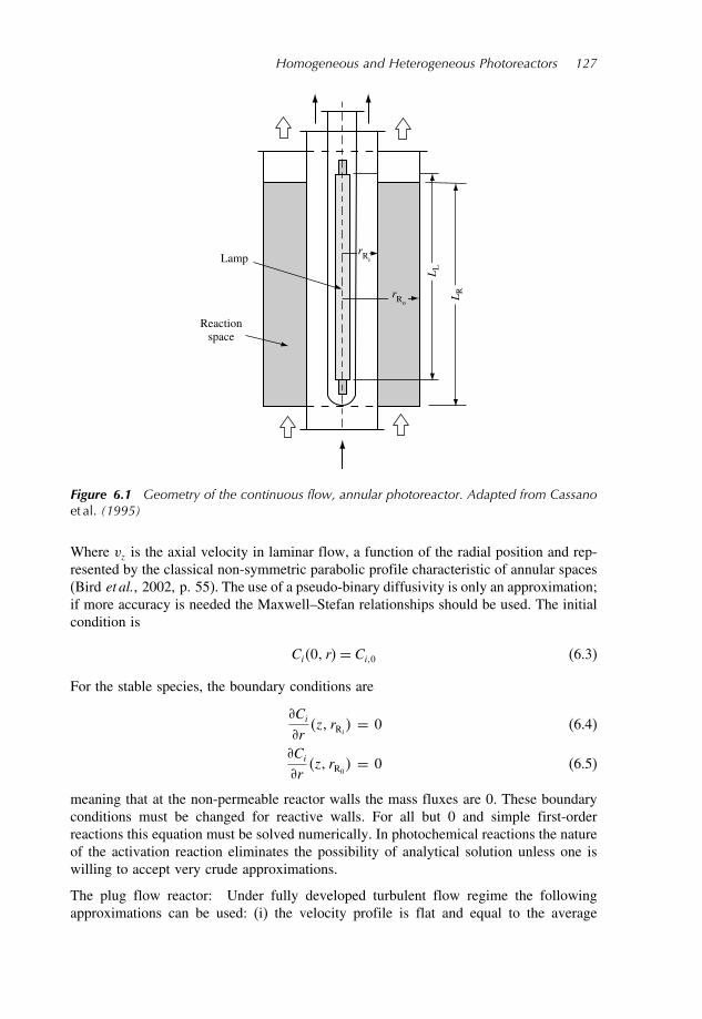
Homogeneous and Heterogeneous Photoreactors 127
rRo
Lamp
Reactionspace
LL
LR
rRi
Figure 6.1 Geometry of the continuous flow, annular photoreactor. Adapted from Cassanoet al. (1995)
Where vz is the axial velocity in laminar flow, a function of the radial position and rep-resented by the classical non-symmetric parabolic profile characteristic of annular spaces(Bird et al., 2002, p. 55). The use of a pseudo-binary diffusivity is only an approximation;if more accuracy is needed the Maxwell–Stefan relationships should be used. The initialcondition is
Ci0 r= Ci0 (6.3)
For the stable species, the boundary conditions are
Cirz rRi = 0 (6.4)
Cirz rR0
= 0 (6.5)
meaning that at the non-permeable reactor walls the mass fluxes are 0. These boundaryconditions must be changed for reactive walls. For all but 0 and simple first-orderreactions this equation must be solved numerically. In photochemical reactions the natureof the activation reaction eliminates the possibility of analytical solution unless one iswilling to accept very crude approximations.
The plug flow reactor: Under fully developed turbulent flow regime the followingapproximations can be used: (i) the velocity profile is flat and equal to the average
128 Chemical Engineering
velocity, and (ii) there is perfect mixing for all stable species in the radial direction.When this is the case and the reactor walls are not permeable, concentration gradients ofstable species in the radial direction can be neglected and equations 6.2, 6.3, 6.4, and 6.5reduce to
vzdCizdz
= Riz rARC (6.6)
Where ARC indicates an average value over the reactor cross-section area. The initialcondition is
Ciz= 0 r= Ci0 (6.7)
It should be specially noted that average values of reaction rates are needed becauseunder no circumstances can photons be very well mixed; consequently, since in the radialdirection in particular the photon concentration is normally non-uniform, usually, thereaction rate will be a strong function of the radial position. This consideration is alsoimportant if the reaction involves highly reactive intermediates, because very often theirreaction characteristic time is much smaller than the hydrodynamic mixing time and thewell-mixed condition cannot be extended to all the species participating in the reaction.Hence, even in approximate models, as is the case for the plug flow simplification, theradiation field non-uniformities cannot be ignored.
The isothermal, constant volume, well-stirred batch reactor. Equation 6.1 can be sim-plified if, due to good mixing conditions, temperature and concentrations are uniform.According to Figure 6.2, integrating in the liquid volume we get
dCitdt
= ⟨RHomix t⟩VR
(6.8)
Note that the reaction rate is still a function of position because the radiation field, alwaysincluded in the reaction rate, is usually not uniform. In equation 6.8:
⟨RHomix t
⟩VR
= 1VR
∫VR
RHomix tdV (6.9)
Even in well-mixed photochemical reactors, the volume average of the reaction ratemust always be calculated because usual experimental measurements never representlocal values. Note that the volume of connecting lines in Figure 6.2 has been considerednegligible. This stirring mechanism is suggested for laboratory reactors to avoid theeffects produced by the presence of a stirrer inside the reactor thus producing a distortionof the radiation field inside the reaction space.
The isothermal, batch reactor with recycle. These systems are normally used when thereaction rate is rather slow and single-pass operation is not effective (Figure 6.3). Underthe following assumptions – (i) differential operation per pass in VR (slow reaction and/orvery high recirculating flow rate), (ii) VR VT, and (iii) very good mixing conditionsin VR and VTk – we can treat the whole system V = VR +VTk as a well-mixed batchreactor. Then, since ·Ni = 0 (no concentration gradients, no inlet or outlet streams),integrating equation 6.1 in the total volume we get
VR+VTk
Unknown︷ ︸︸ ︷dCi x tVT
dt= ⟨RHomi x t
⟩VRVR+
⟨RHomi x t
⟩VTkVTk︸ ︷︷ ︸
Zero: No reaction in the tank
(6.10)

Homogeneous and Heterogeneous Photoreactors 129
Emittingsystem
Reactor
Liquid sampling
Parabolicreflector
Tubular lamp
Pump
h
VR
Figure 6.2 Schematic diagram of the isothermal, constant volume, well-stirred batch reactor
Heat exchanger
Reactor
Pump
Storagetank
Liquidsampling
O2
Parabolicreflector
UV lamph
VR
VTk
Figure 6.3 Schematic diagram of the isothermal reactor with recirculation
The average concentration can be divided into two parts:
VRVT
d Ci x tVRdt︸ ︷︷ ︸
In the reactor
+VTkVT
dCidt︸︷︷︸
In the tank
= VRVT
⟨RHomi x t
⟩VR︸ ︷︷ ︸
Only in the reactor
(6.11)
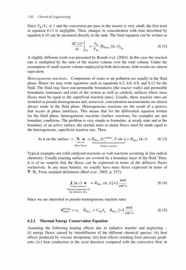
130 Chemical Engineering
Since VR/VT 1 and the conversion per pass in the reactor is very small, the first termin equation 6.11 is negligible. Then, changes in concentration with time described byequation 6.10 can be measured directly in the tank. The final equation can be written as
dCi t
dt
]
Tk
= VRVTk
⟨RHomi x t
⟩VR
(6.12)
A slightly different result was presented by Brandi et al. (2003). In this case the reactionrate is multiplied by the ratio of the reactor volume over the total volume. Under theassumption of small reactor volume employed in both derivations, both results are almostequivalent.
Heterogeneous reactions. Components of water or air pollution are usually in the fluidphase. Hence we may write equations such as equations 6.2, 6.6, 6.8, and 6.12 for thefluid. The fluid may have non-permeable boundaries (the reactor walls) and permeableboundaries (entrances and exits of the system as well as catalytic surfaces where massfluxes must be equal to the superficial reaction rates). Usually, these reaction rates aremodeled as pseudo-homogeneous and, moreover, concentration measurements are almostalways made in the fluid phase. Heterogeneous reactions are the result of a processthat occurs at phase interfaces. This means that for the differential equation writtenfor the fluid phase, heterogeneous reactions (surface reactions, for example) are justboundary conditions. The problem is very simple to formulate: at steady state and at theboundary of an active surface, the normal mass or molar fluxes must be made equal tothe heterogeneous, superficial reaction rate. Then,
At x on the surface→ Ni ·n︸ ︷︷ ︸Mass fluxes
= RHeti
(Csurfacei T etc
)︸ ︷︷ ︸
Surface reaction
= RHeti x t (6.13)
Typical examples are solid catalyzed reactions or wall reactions occurring in free radicalchemistry. Usually reacting surfaces are covered by a boundary layer of the fluid. Then,it is of no surprise that the fluxes can be expressed in terms of the diffusive fluxesexclusively. In any mass balance, we usually have mass fluxes expressed in terms of ·Ni. From standard definitions (Bird et al., 2002, p. 537):
Ji x t ·n︸ ︷︷ ︸Normal component ofthe diffusive flux
= RHeti x t =molcm2 s
(6.14)
Since we are interested in pseudo-homogeneous reaction rates:
RPseudoHomi = av RHeti = CmpSg RHeti =
molcm3 s
(6.15)
6.2.2 Thermal Energy Conservation Equation
Assuming the following heating effects due to radiative transfer and neglecting –(i) energy fluxes caused by interdiffusion of the different chemical species; (ii) heateffects produced by viscous dissipation; (iii) heat effects resulting from pressure gradi-ents; (iv) heat conduction in the axial direction compared with the convective flow in

Homogeneous and Heterogeneous Photoreactors 131
the same direction; and assuming (v) constant physical and transport properties and (vi)steady state conditions – the balance of thermal energy for multicomponent systems incylindrical coordinates is (extracted from Bird et al., 2002, pp. 589, 848)
mixCP
(vzT
z
)
︸ ︷︷ ︸Thermal flow inthe axial direction
= kc[1r
r
(rT
r
)]
︸ ︷︷ ︸Heat conduction in the
radial direction
+ QExt
︸ ︷︷ ︸Radiation
heat sources
− ∑j
Hj Ri
︸ ︷︷ ︸Enthalpy changes
due to chemical reactions
(6.16)
Where QExt is a scalar that includes all forms of heating effects produced by energytransmission without contact, i.e. from external bodies (typically, radiation). In the vastmajority of photochemical reactions (employing visible and UV light), heating effectsproduced by radiation should not be important. However, with lamps emitting significantenergy in the infrared region, if the IR radiation is not filtered (i.e. absorbed by coolingdevices before entering the reactor), the QExt term must be taken into account.
At this point an important consideration concerning photochemical reactions must bestressed. The first step of the reaction – the activation – is made by radiation absorption.The absorbed photons are usually of high energy, producing a change in the electronicstate of the molecule. Thus, the alterations produced in the chemical species are not ofa thermal nature (vibrations, rotations, and translations); i.e. heating effects are almostnegligible. For this reason, for all practical purposes, the radiative transfer equation andthe thermal energy equation can be uncoupled. In equation 6.16, Hj is the partial molarenthalpies of reactants and products. Neglecting heating effects due to radiation, thisequation can be re-written in the more familiar form:
mixCP
(vzT
z
)= kc
[1r
r
(rT
r
)]−∑
j
HjRj x t
︸ ︷︷ ︸Heat of reaction
(6.17)
In equation 6.17, the index j stands for the j different chemical reactions occurring in thesystem. The inlet condition is
T0 r= T0 (6.18)
The boundary conditions that take into account heat transfer from the reactor walls intothe cooling (heating) liquid or vice versa are
kcTz rRi
r= hfT −Tc (6.19)
kcTz rR0
r= −hfT −Tc (6.20)
If the reactor operates under almost isothermal conditions, equations 6.17–6.20 are notneeded. Under plug flow conditions we can integrate equation 6.17 over the cross-sectional area of the tubular reactor and include the boundary conditions into the differ-ential equation. We finally have
mixCP vzdT z
dz+av hf T −Tc︸ ︷︷ ︸
Heat removal
=⟨∑j
(−Hj)Rj x t
⟩
ARC︸ ︷︷ ︸Heat produced
(6.21)

132 Chemical Engineering
6.3 Radiation Transport
When writing the rate of a photochemical reaction it is necessary to make the distinctionbetween dark and radiation-activated (lighted) steps. To treat the dark reactions one usesthe same methodology as for conventional reactors; the main difference appears whenevaluating the rate of the radiation-activated step. The existence of this very particularstep constitutes the main distinctive aspect (and the most important one) between thermal(or thermal catalytic) and radiation-activated reactions. The rate of the radiation-activatedstep is directly proportional to the absorbed, useful energy through a property that has beendefined as the local volumetric rate of photon absorption (LVRPA). The LVRPA, (ea),represents the amount of photons that are absorbed by the reactant per unit time and unitreaction volume. The LVRPA depends on the radiation field (photon distribution) existingin the reaction space; hence, we must know the radiation field within the photoreactor.The value of the LVRPA is defined for monochromatic radiation but it can be extendedto polychromatic fields by performing an integration over all useful wavelengths. Theuseful wavelength range is defined by the overlapping ranges of lamp emission, region ofreactor wall good transmission properties, reactant or catalyst absorption, and, eventually,reflector reflectance (Clariá et al., 1988).The general structure for calculating the rate of the activation step may be illus-
trated schematically as in Figure 6.4. As was shown before, the mass balances requireexpressions formulating the reaction rates; be it a molecular or a free radical reactionmechanism, always some of the steps (generally one) are initiated by radiation absorp-tion. The radiation-activated step kinetics is always written in terms of ea. The evaluationof the LVRPA is performed stating first the general radiation transport equation thatrequires the appropriate constitutive equations for absorption, emission, and scattering.The resulting radiative transfer equation is then successively applied to the reaction space
Radiative transportequation
Constitutiveequations for: – absorption – emission – scattering
Mass balances forstable species
Radiation balance
Application toreactor
and lamp
Reaction rates
Initiation rate
LVRPA
Kinetics ofthe dark reactions
Figure 6.4 Methodology for the evaluation of the rate of the initiation step. Adapted fromCassano et al. (1995)

Homogeneous and Heterogeneous Photoreactors 133
where there is only absorption (in homogeneous media) or absorption and scattering(in heterogeneous media), and to the lamp where emission is the prevailing phenomenon.Combining both results one can obtain, in a straightforward manner, the local value ofthe radiation absorption rate. With this information the rate equation is developed andincorporated into the mass balance.
6.3.1 Spectral Specific Intensity
Under usual conditions, propagation of photons may be represented by bundles of rayswith a given energy. These rays may be specified by the spectral specific intensity that isthe fundamental property for characterizing radiation fields (Figure 6.5). Let dE be thetotal amount of radiative energy passing through the area dA inside the truncated coned in the time dt and with an energy in the wavelength range between and + d.The spectral specific intensity (also called radiance) is defined as
I x t= limdAd dtd→0
(dE
dA cos d dt d
)(6.22)
Quantum theory introduces the proportionality between frequency (or wavelength) andenergy. The energy of a quantum is e = h = hc/. To some extent, a quantum is aunit of energy, but its magnitude is not fixed because it varies with the wavelength (orthe frequency). The best definition of a quantum is that it is the radiant energy equalto h. However it is defined, when one molecule or an atom absorbs one quantum, achange in that molecule or atom from one level of energy to another will be produced;i.e. its energy will have been increased by an amount equal to one quantum. Similarly, ifone mole must reach the same level of activation, the energy absorbed is Nhc/, where
dΩ
dw
dA
n
P
z
y
x
x
o
Ω
θ
Figure 6.5 Characterization of the spectral specific intensity. Adapted from Cassano et al.(1995)

134 Chemical Engineering
N is Avogadro’s number. Hence the energy of a gram mole of a given material willbe increased by Nhc/. The quantity of radiant energy equal to Nhc/ is called oneeinstein. All units in joule (or watt) can be converted into einstein (or einstein s−1) withthe proper transformation. This new unit is very convenient in photochemistry becausethe photochemical activation is the result of the interaction of one molecule with onephoton having one quantum of energy or, in other terms, one mole with one mole ofphotons that have an energy equal to one einstein. The transformation can be obtainedas follows: 1 einstein = 011964/ mWs.
6.3.2 Homogeneous Media
From the radiation viewpoint a homogeneous medium means that scattering does notneed to be considered. This is a great simplification for modeling and design. In this case,the intensity of a monochromatic beam of radiation in any arbitrary direction will bechanged only by emission or absorption. Emission can be usually neglected particularlyfor low-temperature processes. Then, at any point in space x and any time t, we are leftwith the 3D form of the Bouguer–Lambert ‘law’ for monochromatic radiation absorptionin homogeneous media:
dI x tds
+x tI x t= 0 (6.23)
In equation 6.23, s is measured along a chosen direction for photon transport in space . The spectral specific intensity must not be confused with radiation density fluxes.They are equal only for unidirectional irradiation, a case very distant from the generalone. Radiation may be arriving at one point inside a photochemical reactor from alldirections in space. For a photochemical reaction to occur, this radiation must be absorbedby an elementary reacting volume (a material point in space); thus, pencils of radiationcoming from all directions must cross the whole elementary surface that bounds such anelement of volume. Consequently, the important photochemical property is the spectralincident radiation (or spectral spherical irradiance) given by
Gx t=∫ I x td (6.24)
In equation 6.24, integration for all possible directions over the entire sphericalspace has been performed. For polychromatic radiation, integration over the wavelengthrange of interest must be carried out. In the elementary volume of radiation absorption,for single photon absorption, energy is absorbed according to
eax t= x tGx t (6.25)
Where ea is the spectral (monochromatic) LVRPA or the spectral rate of photon energyabsorption per unit reaction volume. Note that since G is a function of position, so is ea.G may be a function of time for lamps operating under unsteady state conditions. Theabsorption coefficient may be a function of position for reactors operating under strongconcentration gradients and a function of time for systems where absorption changeswith the reaction progress (the reactant absorbs radiation, some reaction products absorbradiation, etc.) or when using a photocatalyst the solid semiconductor does not have

Homogeneous and Heterogeneous Photoreactors 135
stable optical properties (fouling or change in particle size). For polychromatic radiationand substituting the differential of the solid angle
ea x t=∫ 2
1
∫ 2
1
∫ 2
1
Ix t sin dd d (6.26)
Where 1 2 and 12 are the integration limits that define the space from whichradiation arrives at the point of incidence. For each point of incidence, in practice, theselimits are defined by the extension of the lamp (its diameter and its length). Thus, toevaluate the LVRPA we must know the spectral specific intensity at each point insidethe reactor. Its value can be obtained from the photon transport equation (equation 6.23).
6.3.3 Heterogeneous Media
In more general terms, the radiative transfer equation may be rationalized consideringa balance of monochromatic photons along a given direction of radiation propagation.Extending a proposal formulated by Whitaker (1977):
∣∣∣∣∣Time rate ofchange of
photons in thevolume V
∣∣∣∣∣+
∣∣∣∣∣∣∣
Net flux of
photons leaving thevolume V acrossits boundingsurface A
∣∣∣∣∣∣∣=∣∣∣∣∣∣
Net gain (loss) of
photons owing to absorptionemission, and in- and out-scattering in the volume V
∣∣∣∣∣∣
t
∫VN dV +
∫AN c ·n dA
= −∫VN a dV +
∫VN e dV +
∫VN s-in dV −
∫VN s-out dV (6.27)
Transforming the area integral, into a volume integral, all the terms will have the sameintegration limits. Then, multiplying by h and considering that I = chN wecan extract the differential equation in terms of specific intensities. In symbolic form(Ozisik, 1973, p. 251)
1c
I t
+ · (I )=−W a
+W e +W s-in
−W s-out (6.28)
Usually the first term can be neglected; i.e. at a given time the radiation field reaches itssteady state almost instantaneously. However I will change with time if the boundarycondition associated with equation 6.28 is time-dependent (typically, a solar reactor) or ifthe state variables which appear in the constitutive equations for any one of the differentprocesses W a
We W
s-in , and W
s-out change with time. Absorption and out-scattering
are modeled in the same way that absorption is accounted for in homogeneous systems.Emission should be modeled according to the particular involved process. However, inmost photochemical reactions it can be neglected because the reaction temperature isusually low and more often than not there is no induced emission (fluorescence and/orphosphorescence). In-scattering is responsible for most of the complications that arisewhen scattering of radiation is an important phenomenon. It results from the almostunavoidable existence of multiple scattering. When scattering is not single, a photon

136 Chemical Engineering
scattered out from one direction may interact with other particles. Then, part of theradiation that is scattered in space in all directions may be incorporated into the streamof photons according to the scattering distribution function (the phase function).For elastic or coherent scattering there is no change in energy; then (Ozisik, 1973, p. 27)
W s-in =
14
∫
′=4
x tp ′ → I ′ x td
′ (6.29)
where p is the phase function. The normalizing condition for the phase function p is
14
∫
′=4
p ′ → d ′ = 1 (6.30)
Scattering is isotropic when p = 1. Isotropic scattering requires, among other require-ments, that at least the scattering material be homogeneous and isotropic, and that thesurrounding medium be also isotropic. More details on scattering and phase functions canbe found in the classical references of Van de Hulst (1957), Ozisik (1973), and Siegeland Howell (1992).Very often the sum of the absorption coefficient and the scattering coefficient is called
the extinction coefficient:
x t= x t+ x t (6.31)
Working photon transport equation. Going back to equation 6.28 one can neglect thetransient term and substitute the different constitutive relationships. After defining adirectional coordinate s along the ray path, from elementary calculus it can be written
dI s t
ds+ s t I s t︸ ︷︷ ︸
Absorption
+ s t I s t︸ ︷︷ ︸Out-scattering
= je s t︸ ︷︷ ︸Emission
+ 14 s t
∫
′=4
p ′ → I ′ s td ′
︸ ︷︷ ︸In-scattering
(6.32)
There is an important assumption implicit in the derivation of this expression; it maybe applied only to a medium that may be considered as pseudo-homogeneous. It shouldhave a valid application when the existing heterogeneities are of small size and theyare present in small concentrations. This consideration leads us to conclude that underthe validity conditions already established for equation 6.32, most likely, conditions forindependent scattering will prevail as well.Perhaps one of the most important conclusions that can be drawn from this equation is
that in heterogeneous reacting systems classical forms of analyzing the light distributioninside the photochemical cell (i.e. the Lambert–Beer equation) are incorrect and, verylikely, useless. To integrate the radiative transfer equation (RTE) we need a boundarycondition: the incoming radiation to the reaction space. It is provided by an emissionmodel for the lamp.

Homogeneous and Heterogeneous Photoreactors 137
6.4 Emission by Tubular Lamps1
6.4.1 The 3D Emission Models
Two main types of models for tubular lamps (the most widely used) will be described.There are lamps that produce an arc that emits radiation and, consequently, photons comeout directly from such an arc. Emission is made by the whole lamp volume. We call thisprocess Voluminal Emission. There are other types of lamps in which the discharged arcbetween electrodes induces an emission produced by some particular substance that hasbeen coated on the lamp surface. We call this process Superficial Emission. Voluminalemission may be safely modeled as an isotropic emission; in this case the specificintensity associated with each bundle of radiation originated in some element of volumeof the lamp is independent of direction, and the associated emitted energy (per unit timeand unit area) is also isotropic (Figure 6.6). On the other hand, it seems that superficialemission can be better modeled by a diffuse type of emission that is also known as onethat follows the Lambert’s ‘cosine law’ of emission; in this case the emitted intensityis independent of direction but the emitted energy depends on the surface orientationand follows the ‘cosine law’ equation (Figure 6.7). The following assumptions are made(Irazoqui et al., 1973):
1. The emitters of the radiation source are uniformly distributed over the region ofemission (a volume or a surface).
2. In terms of Specific Intensities each elementary extension of emission has an isotropicemission but the outgoing radiation energy is: (i) isotropic when the emitting elementis a volume or (ii) diffuse (affected by the surface orientation) when the element is asurface.
s = sR
s = sS
ρ = ρ1
ρ = ρ2
s = 0
I
z
rRL
dφ
dVe
dθReactor
Lamp
φ
θ
Figure 6.6 The extended source with the voluminal emission model for the lamp. Adaptedfrom Cassano et al. (1995)
1 Reprinted with permission from Cassano et al., 1995, Copyright 1995 American Chemical Society.

138 Chemical Engineering
Reactor
z
yx
RL
d Ae
I
dφ
dθ
n
s = sR
ρ = ρi
s = sS
ρ = ρeθm
θ
φ
Figure 6.7 The extended source with the superficial emission model for the lamp. Adaptedfrom Cassano et al. (1995)
3. Any emission element of the lamp emits per unit time, and for a given wavelengthinterval, an amount of energy proportional to its extension and independent of itsposition inside the lamp volume or on the lamp surface.
4. When emission is voluminal, each of the differential volumes of emission is transparentto the emission of its surroundings (a possible questionable approximation).
5. The lamp is a perfect cylinder bounded by mathematical surfaces with zero thickness.Hence, any bundle of radiation coming from inside does not change its intensity ordirection when it crosses this boundary (again, an approximation).
6. The lamp is long enough; consequently, neglecting end effects, the emission producedby the lamp along its central axis is uniform. This assumption does not imposeuniformity on the radiation field generated along the direction of the central axis.
Three-dimensional source with superficial diffuse emission. The E-SDE source model.From the lamp surface s = sS to the reactor wall s = sR there is no emission(Figure 6.7), no scattering, and no absorption (the medium is assumed to be diactinic);therefore,
dIs ds
= 0 (6.33)
It follows that
I0= Ix =i = Ix =e R (6.34)
Since emission is uniform in space and isotropic in directions
Ix =e = Ie (6.35)

Homogeneous and Heterogeneous Photoreactors 139
Now we must relate the value of the specific intensity of emission to the emissionpower of the lamp. From the definition of the spectral specific intensity
dPS = Ie d dAe cosn (6.36)
from which
Ie =PS∫
Scosn d
∫ASdAe
= PS22RLLL
(6.37)
According to equations 6.34, 6.35, and 6.37, the boundary condition when a lamp withsuperficial emission is used is given by
I0 =R PS22RLLL
(6.38)
Three-dimensional source with voluminal isotropic emission. The E-VIE source model.Since emission is produced by a volume, the radiative transfer equation can be appliedinside the lamp. There is no absorption (assumption 4) and no scattering. For isotropicand uniform emission
dIs tds
= jes t= je (6.39)
Along the direction , at s = 0 (Figure 6.6), there is no entrance of radiation; thissituation provides the required boundary condition for equation 6.39:
s = 0 I0 = 0 (6.40)
Integrating from s = 0 to s = sS and changing coordinates (recall Figure 6.6):
s = 0 = 2 (6.41)
s = sS = 1 (6.42)
and one gets:
Iss = jesx = 2x −1x (6.43)
It must be remarked that, as should have been expected, s is a function of the positionx inside the reactor and the direction of the incoming radiation given by the sphericalcoordinates . Once more, from s = sS to s = sR there is no emission, no scattering,and no absorption; from assumption 5 there is no refraction or reflection at the lampboundaries, therefore
dIs ds
= 0 (6.44)
Consequently, the boundary condition is
I0= jesx R (6.45)

140 Chemical Engineering
Once more, the value of je must be related to the lamp output power Ps. By definition,je is the energy emitted per unit volume, unit solid angle of emission, and unit time;therefore
Ps =∫ S
∫VS
je dVe d (6.46)
Since je corresponds to an isotropic and uniform emission
je =Ps
42R2LLL
(6.47)
From equation 6.43 we must know the values of 2x and 1x . In orderto know these values one must obtain explicit expressions for the independent variable ,at the positions indicated by equations 6.41 and 6.42. To illustrate the procedure, the caseof an annular reactor will be analyzed (Figure 6.8). Let us consider a point located in anarbitrary position I, having coordinates xr z and look at an arbitrary direction .The equation of the boundary surface of the radiation source (a cylinder) in sphericalcoordinates is written as follows:
2 sin2 −2sin cosr+ r2−R2L= 0 (6.48)
The two solutions of this quadratic equation are precisely the values of ; i.e. they arethe intersections of the coordinate with the front and rear parts of the lamp at any valueof and :
12 =r cos± r2 cos2− r2+R2
L1/2
sin (6.49)
Finally, the following value for S is obtained:
S =2[r2cos2−1+R2
L
]1/2sin
(6.50)
The boundary conditions when a lamp with voluminal emission is employed results in:
I0x =PSR
22R2LLL
[r2cos2−1+R2
L
]1/2sin
(6.51)
I
1 2 3
ρ I(θ,φ)ρ i(θ,φ)
ρ1(θ,φ)ρ 2(θ,φ)
x
Figure 6.8 The annular reactor. Adapted from Cassano et al. (1995)

Homogeneous and Heterogeneous Photoreactors 141
Limits of integration for the 3D emission models. When a lamp with superficial emissionis used, according to equation 6.38, a constant value must be incorporated as a boundarycondition. Conversely, when lamps with voluminal emission are used, according toequation 6.51, the boundary condition introduces a function of x , and . The limits ofintegration for the annular reactor with the tubular lamp were derived by Irazoqui et al.(1973) and systematically described by Cassano et al. (1995). They are
1= tan−1
r cos− [r2cos2−1+R2
L
]1/2LL− z
(6.52)
2= tan−1
r cos− [r2cos2−1+R2
L
]1/2−z
(6.53)
−1 = 2 = cos−1
[r2−R2
L1/2
r
](6.54)
The limits of integration for the case in which reflecting surfaces are present in thesystem (for example elliptical or parabolic reflectors) require a more elaborated procedure(Cassano et al., 1995).
6.5 Homogeneous Systems. Reaction Kinetics of a PollutantPhotolysis and its Application to the Predictionof the Performance of an Annular Reactor 2
6.5.1 Reaction Kinetics
A very simple case will be used to illustrate the procedure. For many processes employingradiation having a wavelength below 300 nm, direct photolysis is often present. Hence,even if in practice an oxidant will always be used (for example, hydrogen peroxide) theparallel photolysis must be also modeled. 2,4-dichlorophenoxyacetic acid (2,4-D) is awidespread herbicide that is known to have a high level of toxicity. The reaction usingUV alone with 2,4-D shows most of the features that must be taken into account tomodel a homogeneous reactor for AOTs. Although it is a rather slow reaction that needsto be complemented with a stronger oxidation, it can be used to illustrate some of theconcepts previously developed. As reported by Cabrera et al. (1997a), kinetic studies wereperformed in a well-stirred, batch, cylindrical photoreactor irradiated from the bottom(Figure 6.2). Monochromatic light (= 254nm) was used. Analyses of the results wereperformed as is described in the following sections.
Radiation field. Alfano et al. (1985) studied the above described reactor geometry usinga 3D (r, z, ) model. It was found that for the used geometry and dimensions, radialand angular variations were not very significant. With this background, a 1D model(x-coordinate) can be adopted. Then, incident radiation (equation 6.24) can bedescribed by
Gx=GW exp(−Tx
)(6.55)
2 Reproduced with permission from Cabrera et al., 1997a and Martín et al., 1997; Copyright 1997 IWA Publishing.
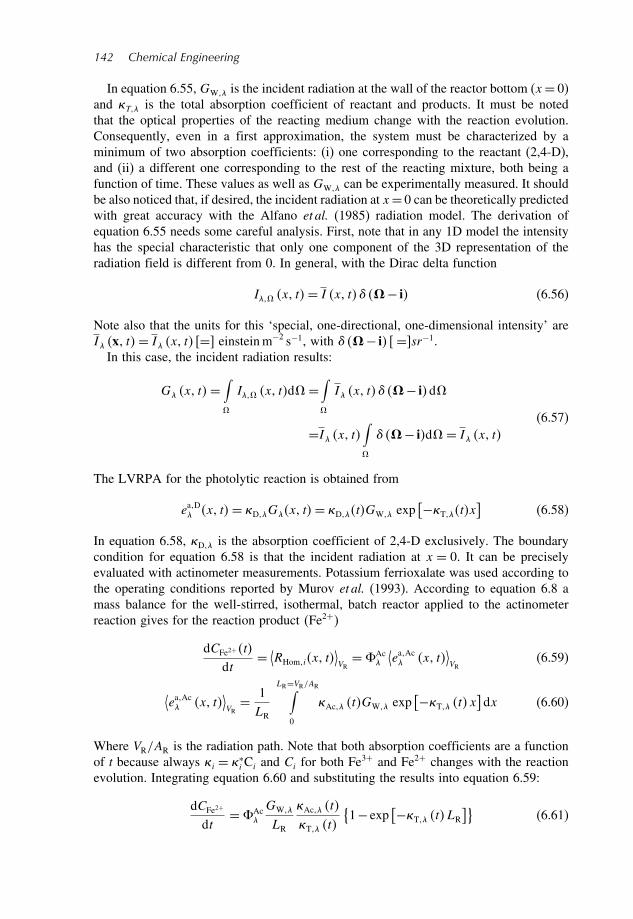
142 Chemical Engineering
In equation 6.55, GW is the incident radiation at the wall of the reactor bottom (x= 0)and T is the total absorption coefficient of reactant and products. It must be notedthat the optical properties of the reacting medium change with the reaction evolution.Consequently, even in a first approximation, the system must be characterized by aminimum of two absorption coefficients: (i) one corresponding to the reactant (2,4-D),and (ii) a different one corresponding to the rest of the reacting mixture, both being afunction of time. These values as well as GW can be experimentally measured. It shouldbe also noticed that, if desired, the incident radiation at x= 0 can be theoretically predictedwith great accuracy with the Alfano et al. (1985) radiation model. The derivation ofequation 6.55 needs some careful analysis. First, note that in any 1D model the intensityhas the special characteristic that only one component of the 3D representation of theradiation field is different from 0. In general, with the Dirac delta function
I x t= I x t − i (6.56)
Note also that the units for this ‘special, one-directional, one-dimensional intensity’ areI x t= I x t [=] einsteinm−2 s−1, with − i [=sr−1.
In this case, the incident radiation results:
G x t=∫
I x td =∫
I x t − id
=I x t∫
− id = I x t(6.57)
The LVRPA for the photolytic reaction is obtained from
eaD x t= DGx t= DtGW exp[−Ttx
](6.58)
In equation 6.58, D is the absorption coefficient of 2,4-D exclusively. The boundarycondition for equation 6.58 is that the incident radiation at x = 0. It can be preciselyevaluated with actinometer measurements. Potassium ferrioxalate was used according tothe operating conditions reported by Murov et al. (1993). According to equation 6.8 amass balance for the well-stirred, isothermal, batch reactor applied to the actinometerreaction gives for the reaction product Fe2+
dCFe2+t
dt= ⟨RHomix t
⟩VR
=Ac
⟨eaAc x t
⟩VR
(6.59)
⟨eaAc x t
⟩VR
= 1LR
LR=VR/AR∫
0
Ac tGW exp[−T t x
]dx (6.60)
Where VR/AR is the radiation path. Note that both absorption coefficients are a functionof t because always i = ∗iCi and Ci for both Fe3+ and Fe2+ changes with the reactionevolution. Integrating equation 6.60 and substituting the results into equation 6.59:
dCFe2+
dt=Ac
GW
LR
Ac t
T t
1− exp
[−T tLR
](6.61)

Homogeneous and Heterogeneous Photoreactors 143
In equation 6.61, Ac is the reactant(Fe+3
)and the reaction product is Fe+2. In the batch
reactor, for not too high reactant conversions, the plot of Fe+2 concentration versus timegives a straight line. Then, at t→ 0 and taking into account that at 254 nm Fe3+ is large:
GW =(VR
Ac AR
)limt→0
(CFe2+ −C0
Fe2+
t−0
)(6.62)
2,4-D mass balance. The reactor operates under the following conditions: (i) perfectmixing, and (ii) isothermal performance. The mass balance (equation 6.8) gives
dCDt
dt= ⟨RD y t
⟩LR
CDt = 0= C0D
(6.63)
An expression for the local reaction rate is still unknown. The following simple relation-ship was proposed:
RD y t=−D
[eaD y t
]nCDt
m (6.64)
Calculating the average reaction rate and substituting into the mass balance, after inte-gration:
dCDt
dt=− 1
LR
D
(GW
)n(Dt
)nTtn
CDtm1− exp
[−TtLRn]
(6.65)
This ordinary differential equation must be solved with the initial condition indicated inequation 6.63. Note that due to the required averaging procedure, the reaction order withrespect to the LVRPA (n) has a rather complex relationship with respect to the time rateof change of concentrations.
Absorption coefficients. Equation 6.65 needs two optical parameters that must beobtained from independent measurements. The 2,4-D absorption coefficient can beobtained from standard measurements. To obtain the total absorption coefficient (a mix-ture of reactant and reaction products), it was proposed:
Tt= ∗DCDt+∗PrCPrt (6.66)
The ‘unknown-products’ hypothetical concentration can be expressed in terms of the2,4-D instantaneous concentration:
Tt= ∗DCD t+∗Pr(C0
D−CD
)= (∗D−∗Pr)CDt+∗PrC0
D (6.67)
With experimental information the following empirical correlation was obtained:
Tt= 00197C0D−001785CDt (6.68)

144 Chemical Engineering
Parameter evaluation. It is now possible to obtain the kinetic parameters from the exper-imental data and the proposed kinetic model in equation 6.64. We have three unknowns:the quantum yield, and the exponents ‘m’ and ‘n’. The whole model (equation 6.65)was fed to a multiparameter, non-linear regression algorithm that is coupled with anoptimization program according to the Marquardt method (Marquardt, 1963). The regres-sion program gave the following values for the exponents: n 1 and m 0. With theseestimations, at 25C and 253.7 nm, the following kinetic equation was obtained:
RDy t=−00262eaD y t (6.69)
This result should not be interpreted as zero-order dependence with respect to 2,4-Dconcentration because it participates in two parts of the variable eaD (see equation 6.58).
6.5.2 Reactor Analysis
A pilot plant scale, tubular (annular configuration) photoreactor for the direct photolysisof 2,4-D was modeled (Martín et al., 1997). A tubular germicidal lamp was placed at thereactor centerline. This reactor can be used to test, with a very different reactor geometry,the kinetic expression previously developed in the cylindrical, batch laboratory reactorirradiated from its bottom and to validate the annular reactor modeling for the 2,4-Dphotolysis. Note that the radiation distribution and consequently the field of reaction ratesin one and the other system are very different.
Proposed reactor (pilot plant scale). Figures 6.1 and 6.3 (the reactor substituted by theannular tube of Figure 6.1) provide a schematic representation of the employed reactingsystem. More details can be found in Table 6.1.
Reactor model. The reactor model was constructed according to the following sequence:(i) the annular reactor, radiation distribution model of Romero et al. (1983) was adaptedfor this particular set-up; (ii) the tubular lamp with voluminal and isotropic radiationemission model was applied to this system; (iii) a mass balance for an actinometricreaction carried out in a tubular reactor inside the loop of a recycling system wasadapted from Martín et al. (1996); and (iv) the verification of the radiation model,actinometer experiments were performed in the reactor to compare theoretical predictions
Table 6.1 Reacting system and lamp characteristics. Reproducedwith permission from Martín et al. (1997) copyright 1997, IWAPublishing
Parameter Value Units
REACTOR Irradiated length 48 cmPyrex® Outside diameter 603 cmSuprasil® Inside diameter 445 cm
Irradiated volume 624 cm3
LAMP Input power 30 WPhilips TUV Output power 9 W= 2537nm Nominal length 895 cm
Diameter 26 cmRESERVOIR Volume 6000 cm3

Homogeneous and Heterogeneous Photoreactors 145
with actual results. This procedure permitted the verification of the quality of the radiationemission model for the lamp and the radiation distribution model for the annular reactor.Afterwards, for the photolytic reactor employing 2,4-D, the following sequence wasfollowed: (1) a species mass balance for a tubular reactor inside the recycling system waswritten according to equation 6.12; (2) the kinetic expression given by equation 6.69 wasincorporated into this mass balance; (3) the radiation model previously validated was usedto predict the LVRPA in the kinetic expression (equation 6.69); (4) radiation absorptionby reactants and products was incorporated into the radiation model according to theempirical expression represented by equation 6.68; (5) time evolution concentrations ofthe 2,4-D in the recycling system were predicted using steps (1), (2), (3), and (4); and(6) experimental 2,4-D concentrations in the pilot plant reactor were compared withtheoretical predictions.
Radiation field. For a homogeneous medium the radiation distribution is obtained bysolving equation 6.23 with the following boundary condition:
I s = 0= I0 (6.70)
The boundary condition was obtained from the 3D with voluminal and isotropic emissionmodel (equation 6.51). The solution of equation 6.23 provides values of the radiationintensity as a function of position (r, z) and direction . Once I is known, theincident radiation and the LVRPA can be obtained from equations 6.24 and 6.25. Sincemonochromatic radiation is employed, no integration over wavelength is needed. Thefinal equation for calculating the LVRPA is
eax t=ix tR P
22R2LLL
2∫
1
d
2∫
1
dR2L− r2 sin21/2
× exp[−T
(r cos− r2 cos2− r2− r2Ri1/2
sin
)] (6.71)
The integration limits for and for the case of the annular reactor are described byequations 6.52, 6.53, and 6.54. It must be noticed that the exponential term (attenuation)uses the reacting medium total absorption coefficient while only the reactant absorptioncoefficient intervenes, with a linear effect, in the value of the LVRPA. Hence i standsfor the reactant.The actinometer reaction in the annular reactor: The classic uranyl oxalate reaction was
used (Murov et al., 1993). According to Brandi et al. (2003), changes in concentrationinside the recycling system were obtained from
dCitdt
]
Tk
= VRVT
RHomAcr z tVR (6.72)
Ci0= C0i
RHomAc r z t=−AceaAc r z t (6.73)

146 Chemical Engineering
Calculating the volume average of the LVRPA we get
⟨eaAc x
⟩VR
=AcRPR2
LLLVR
rRo∫
rRi
r dr
LR∫
0
dz
2∫
1
d
2∫
1
dR2L− r2 sin21/2
× exp
[−Ac
(r cos− (r2 cos2− r2− r2Ri
)1/2sin
)] (6.74)
In this reaction, the concentration of the absorbing species remains constant for conver-sions below 20% (sensitized reaction). To validate the radiation model, results obtainedfrom equation 6.74 must be compared with experiments. From equations 6.72 and 6.73and after integration, the experimental value of the LVRPA is
[eaAc
]Exp
= C0Ac−CAct
t−0VTVR
1Ac
(6.75)
Experiments were carried out at three different uranyl sulfate concentrations: 0.005,0.001, and 0.0005M. Oxalic acid concentrations were always five times larger. Thelargest error between model and experiments was smaller than 8%. Since agreement isvery good, one may conclude that the radiation field of the annular reactor has beenprecisely represented. Note that no adjustable parameters have been used and the boundarycondition was obtained with a theoretical model.
The reactor model for the 2,4-D photolysis. The simplified kinetic expression repre-sented by equation 6.69 has the same form as equation 6.73. However, during the 2,4-Dphotolysis the radiation absorption characteristics of the reacting medium change. Thisis a very distinct phenomenon because (i) the uranyl oxalate reaction is a photosensitizedreaction and the radiation absorbing species is not consumed, and (ii) conversely, not onlythe 2,4-D absorption coefficient changes, but absorption by reaction products increasesthe total absorption coefficient above the initial value. This phenomenon produces anunavoidable coupling between the steady state radiation balance and the unsteady statemass balance. The total absorption coefficient can be obtained from equation 6.68. Then;
dCDt
dt= VRVT
RHom,Dr z tVR (6.76)
with the I.C. CDt = 0= C0D (6.77)
The reaction rate is
⟨RHom,D r z t
⟩VR
=−D
1VR
∫VR
ea,D r z tdV (6.78)

Homogeneous and Heterogeneous Photoreactors 147
Inserting the LVRPA into equation 6.78 and substituting the result into equation 6.76we obtain
dCD
dt=−D
1VT
[PR
∗DCDt
R2LLL
] rR0∫
rRi
r dr
LR∫
0
dz
2∫
1
d
2∫
1
dR2L− r2 sin21/2
exp
−T
(r cos− (r2 cos2− r2− r2Ri
)sin
)1/2
CDt = 0= C0D
(6.79)
Integration of this equation provides the time evolution of the 2,4-D concentration. Noticethat all the lamp characteristics are incorporated in the design equation. The mass balanceand the volume average procedure indicated in the equations above are greatly simplifiedby the differential operation in the photochemical section of the reactor. Figure 6.9 showsthe results for two initial concentrations. Solid lines correspond to predictions of the2,4-D concentrations obtained from the solution of equation 6.79. Symbols correspondto experimental values. It can be seen that agreement is fairly good. The observeddiscrepancies, which in some cases produce an error as large as 15%, are mainly dueto the fact that the reaction kinetics of this very complex reaction has been modeled interms of just one single variable (the 2,4-D concentration).The ideas described in this section can be easily extended to more complex reacting
systems either from the chemistry point of view – for example to include the paralleloxidation reaction with hydrogen peroxide or ozone – or to deal with other lamp-reactor configurations. A comprehensive, tutorial review for homogeneous photochemicalreactors has been published (Cassano et al., 1995) that provides most of the requiredmethods.
0 2 4 6 8 10t [h]
0
20
40
60
80
100
CD
[ppm
]
Figure 6.9 Results of the scale-up procedure for the 2,4-D degradation process. Modelpredictions (–); experimental data (O). Reproduced with permission from Martín et al.(1997) copyright 1997, IWA Publishing

148 Chemical Engineering
6.6 Heterogeneous Systems
For the case of photocatalytic reactors employing solid semiconductors and trying to reacha compromise between length and clarity in a detailed application, it seems appropriate toconcentrate effort on describing all the reactor analysis concepts that must be developedto measure (i) true quantum yields in heterogeneous slurry photoreactors, and (ii) specificprocedures to obtain intrinsic kinetic models in laboratory reactors. These conceptscan be immediately extended to the design of the reactor because (1) the models forthe lamp emission are the same as the ones described in homogeneous systems and(2) the modeling of the reactor can, at most, include some additional complications whenscattering has to be described in cylindrical geometries (Romero et al., 1997, 2003).The problem of true quantum yield determination allows us to show in a rather shortextension most of the main features of heterogeneous photocatalytic reactor modeling(Brandi et al., 2003). How to incorporate a complex reaction scheme or mechanism intothe corresponding mass balance, as has been shown by Alfano et al. (1997) and Cabreraet al. (1997b), will be also presented. Once the distribution of radiation inside reactorsof different geometries is known (see e.g. Romero et al., 2003, for annular reactorsand Brandi et al., 1999, for flat plate reactors), basic concepts already available in thechemical reactor engineering literature can be used to model other reactions and reactortypes.
6.6.1 True Quantum Yield Evaluation in Slurry Reactors
The general methodology for modeling slurry photoreactors has been reviewed byCassano and Alfano (2000). We will apply these concepts to the evaluation of absolute,true values of quantum yields.
Definition of the problem. The monochromatic, overall, true initial quantum yield isdefined as
[0
]TRUE
=
[Rate of
disapearanceappearence
of compound ‘i’x t
]t → 0
VR−AVER
Rate of photon absorption by the catalystx tVR−AVER
=[Ri0VR
]EXPER[
eaVR]CALC
(6.80)
The volume average of the LVRPA is very difficult to measure. However, employingrigorous mathematical modeling of photocatalytic slurry reactors it can be preciselycalculated (Brandi et al., 2000a,b). Consequently, in equation 6.80, (i) the numerator isthe reactor volume-averaged of the reaction rate measured at initial conditions (the resultof an experimental determination), (ii) the denominator is the reactor volume-averagedof the calculated spatial distribution of the LVRPA, and (iii) the LVRPA is calculatedsolving the radiative transfer equation (RTE) employing catalyst optical properties andlight intensities arriving at the reactor window for radiation entrance, both independentlymeasured.
Homogeneous and Heterogeneous Photoreactors 149
Quantum yields are not unique values unless several operating conditions are preciselydefined, for example:
1. Concerning the employed radiation, wavelength must be monochromatic and theemployed range of radiation intensities must be defined because of the existence ofdifferent reaction order dependencies at different irradiation rates.
2. Concerning the reaction environment, several conditions must be fixed: temperature,pH, substrate initial concentration, and quality of the ‘reactants’ that are employedbecause impurities affect the photocatalytic rates.
3. Concerning the oxidative path, operating conditions must ensure excess oxygen con-centration over the stoichiometric demand during the full course of the reaction.
4. Concerning the catalyst, we must define catalyst variety and catalyst concentration.5. If there is simultaneous homogeneous photolysis, it must be treated as a parallel
reaction to exclude its effects from the photocatalytic ones.
Additionally, to facilitate comparisons, quantum yields should be measured at substrateand catalyst concentrations where the reaction rate shows zero-order dependence withrespect to both variables.
Methodology. To develop a rigorous model of a photocatalytic slurry reactor severalsteps were necessary. They are briefly described below.
1. To study scattering effects by solid particles in a fluid and adapt previous exist-ing methods in generalized transport theory (the discrete ordinate method or DOM)(Duderstadt and Martin, 1979) to solve the RTE (Alfano et al., 1995).
2. To develop a laboratory reactor that permits the easiest solution of the RTE employingthe DOM (Cabrera et al., 1994). It consists of a flat plate configuration (a cylinderirradiated from one of its circular surfaces).
3. To develop special methods to measure monochromatic specific (per unit catalystmass) absorption ∗ and scattering ∗
coefficients of titanium dioxide slurries andobtain values for different catalysts and for the wavelength range of interest (Cabreraet al., 1996).
4. To develop precise methods for obtaining intrinsic kinetic data in a batch reactor withrecycle (Alfano et al., 1997; Cabrera et al., 1997b).
5. To include the effects of reactor wall properties into the incident radiation intensitiescorresponding to the boundary condition for radiation entrance. The model includesinternal absorption and interfacial reflectivities (Brandi et al., 1999).
6. To characterize and model the problem of reactor window fouling by titanium dioxide(Brandi et al., 1999).
7. To select the best phase function for radiation scattering by titanium dioxide (Brandiet al., 1999).
8. To obtain direct and precise experimental verification of the quality of the resultsobtained with the numerical solution of the RTE with the DOM (Brandi et al., 2000a,b).For catalyst loadings above 0.25 g/L, errors were never larger than 5%.
Selection of a reactor. At this point we should decide on the experimental reactor tobe used. Cabrera et al. (1994) proposed a new experimental reactor that – with a few

150 Chemical Engineering
xx
IIλI0,λ
Reactor
Pyrex window
Ground glass
Parabolicreflector
Tubularlamp
Ref.
Dirθ
Figure 6.10 Schematic description of the uni-dimensional photocatalytic reactor. Adaptedfrom Cassano and Alfano, 2000
changes – has been successfully used for detailed kinetic studies. Figure 6.10 gives aschematic description of the device. It consists of the following parts:
1. A cylindrical reactor with two flat windows made of good quality Pyrex glass (alter-natively, one of them may be made of Suprasil quality quartz). The window forradiation entrance – either glass or quartz – must be modified; its external side uponabrasion with HF has the texture of ground glass. The reactor has an optical path LRsufficiently large to ensure that no radiation is arriving at the flat plate facing thewindow of radiation entrance. Illuminating the reactor through the modified windowproduces diffuse irradiation inside (the irradiation boundary condition) which greatlysimplifies the radiation model (Figure 6.10).
2. A tubular UV lamp of well-known characteristics: output power, radiation spectraldistribution of its output energy, and geometrical dimensions. This lamp has significantpeaks of emission at 313 and 365 nm.
3. A cylindrical reflector of parabolic cross-section with well- known reflecting properties(Alzac®Aluminum from Alcoa) and well-defined geometrical dimensions.
4. Monochromatic light was obtained by interposing in the radiation bundle trajectoriesnarrow band interference filters (peaks at 313 and 365 nm).
5. A shutter placed in front of the reactor window allowed us to decide on the exactstarting time of the reaction once steady state conditions had been reached.
The reacting system was operated inside the loop of a batch recycling arrangement(Figure 6.3) with provisions for (1) a storage tank, (2) an all-glass and Teflon recirculatingpump with high flow rate capacity, (3) a temperature control system, and (4) a continuousfeed for oxygen. A laboratory reactor must be constructed in such a way that an exactanalysis of the experimental results should be simplified as much as possible. Thisexperimental device has four important features for its modeling: (1) the tank volume issignificantly larger than the reactor volume; (2) the pump has a high flow rate, thus inthe reactor, conversion per pass will be very small; (3) irradiation at the inside face ofthe reactor window is diffuse which means that azimuthal symmetry for the direction of

Homogeneous and Heterogeneous Photoreactors 151
radiation propagation inside the reactor will be achieved; and (4) no radiation arrives atthe opposite face of the reactor plate and consequently there is no radiation reflection onthis face.
Calculating procedure for the reaction rate3. On this occasion we will use the con-cepts already derived in section 6.2. Consider the case represented in Figure 6.3. Fromequation 6.1, a local mass balance for the i component in the liquid where there is nochemical reaction (no parallel photolysis) is
Cix tt
+ ·Ni = 0 (6.81)
This equation can be integrated over the whole liquid volume of the system VLTthat, in principle, is different from the total volume of the suspension (liquid + solid)VTot = VTk +VR = VLT+VST. Defining
Cix tVLR =1VLR
∫
VLR
Cix tdV (6.82)
we get
∫
VLT
Cix tt
dV = VLRddt
Cix tVLR +VLTkdCitdt
∣∣∣∣Tk
(6.83)
∫
VLT
·Ni dV =∫
AST
Jix t︸ ︷︷ ︸
Diffusion
+Cix tv︸ ︷︷ ︸Convection
·nL dA (6.84)
We have considered that ALT = AST; i.e. the total interfacial area of the liquid isequal to the total interfacial area of the solid. Noting that fluxes are different from 0 onlyat permeable solid surfaces, in a closed system the only permeable surfaces are thosecorresponding to the catalyst. Therefore;
VLRddt
Cix tVLR +VLTkdCitdt
=−AST Jix t ·nLAST−∫
AST
Cix tv ·nL dA(6.85)
In equation 6.85, Ji x t ·nLAST is ‘the total liquid–solid particles interface, averaged,molar diffusive flux of component i’. Note that AST = ASR +ASTk. The second termof the right-hand side of equation 6.85 is 0 because at the catalyst interface convectivefluxes are 0. On the other hand, from equation 6.13 the molar diffusive flux throughthe boundary layer at the liquid–solid interface must be equal to the reaction rate at theliquid–solid interface:
AST Ji x t ·nLAST = ASR Ji x t ·nLASR =−ASR
⟨RHeti x t
⟩ASR
(6.86)
3 Extracted and reprinted with permission from Cabrera et al., 1997b, Copyright 1997, Elsevier.

152 Chemical Engineering
Substituting equation 6.86 into equation 6.85:
LVRVTk
d Ci x tVLRdt
+LdCitdt
= VRVTkaV⟨RHetix t
⟩ASR
(6.87)
where L is the liquid hold-up in the system that is uniform throughout and aV is thecatalytic surface area per unit suspension volume. Since VR/VTk < 1 and the conversion
per path in the reactor[dCixtVLR
dt
]is very small (both being design conditions);
LdCitdt
∣∣∣∣Tk
= VRVTkaV⟨RHetix t
⟩ASR
(6.88)
⟨RHetix t
⟩ASR
= L1
SgCmp
VTkVR
dCitdt
∣∣∣∣Tk
= molcm2 s
(6.89)
When the same value per unit suspension volume is needed (for equation 6.80) we mustconsider that (i) the cross-sectional area corresponding to the irradiated flat plate reactoris constant (a design condition), and (ii) the catalyst concentration is uniform (well-mixedsystem in the whole reactor volume; an established operating condition):
⟨RPseudo
Homi x t⟩VR
= ⟨RPseudoHomi x t
⟩LR
= LVTkVR
dCitdt
∣∣∣∣Tk
= molcm3 s
(6.90)
Equation 6.90 provides the value of the numerator of equation 6.80.
Photon absorption rate by a material particle of the suspension4. At this point we wouldlike to know the LVRPA by the solid and to be able to isolate this value even if theliquid would also absorb radiation. To do this we need to model absorption by a materialparticle of the suspension. In the continuum mechanics sense, a material point in space isa volume for which every property can be well defined by a single value. For a catalyticsuspension, it will be made of the liquid and the solid phases. Let us consider a smallvolume V of the suspension space representing this material particle. This volume islocated at a point in space x (Figure 6.11). Any point inside V can be defined in termsof a local reference frame .We must now relate the LVRPA per particle, Ea
Snx+ t, to the LVRPA by thesuspension volume (liquid + solid), eax t. The absorbed energy per unit wavelengthinterval, unit time, and unit volume of the suspension (solid plus liquid) is by definitionof an average value over the total volume:
eax t=1V
∫
V
dVeax+ t (6.91)
where V is the small suspension volume of the heterogeneous system (solid plus liquid)located at point x. The right-hand side of equation 6.91 can be divided into two parts: (i)the radiation energy absorbed by the liquid, and (ii) that part of the absorbed radiation
4 Extracted and reprinted with permission from Alfano et al., 1997, Copyright 1997, Elsevier.

Homogeneous and Heterogeneous Photoreactors 153
P
V = VL + VS
Liquid
IntensitySmall suspensionvolume
Solid particle
x
x1
x2
x3
nS
nL
ζζ
3
ζ3
ζ2
ζ2
ζp
ζ1
ζ1
Figure 6.11 Modeling of photon absorption by a material particle of the suspension.Adapted from Alfano et al. (1997)
corresponding to the solid particles. Additionally, suppose that in the small volume Vwe have N solid photocatalytic particles:
eax t=1V
∫
VL
dVeaLx+ t+1V
N∑n=1
∫
VSn
dVeaSx+ t︸ ︷︷ ︸Absorption by one particle
(6.92)
Assuming that on average all particles are equal:
ea x t =L⟨eaLx+ t
⟩VL︸ ︷︷ ︸
Average value of absorptionby the liquid phase
+ NV︸︷︷︸Number of particlesper unit volume
∫
VSn
dVeaSx+ t︸ ︷︷ ︸Absorption by one particle
(6.93)
In this equation, L is the liquid hold-up VL/V and NV =N/V is the number of particlesper unit suspension volume. Finally, from equation 6.93 we get
EaSnx t NV︸ ︷︷ ︸
Absorption by the solid
=
eax t︸ ︷︷ ︸
Total absorption
−L⟨eaLx+ t
⟩VL︸ ︷︷ ︸
Absorption by the liquid
(6.94)
If the liquid does not absorb radiation in the wavelength range under consideration, thesecond term of the right-hand side is 0. When the liquid is transparent, equation 6.94

154 Chemical Engineering
indicates that the solution provided by the RTE in terms of the absorption and scatteringcoefficients of the suspension can provide, directly, the value of the photon absorptionrate by solid particles. Consequently, if the liquid is transparent,
eaSol x t︸ ︷︷ ︸Absorption by
the solid particles
= NV EaSn x t= ea x t︸ ︷︷ ︸
Solution of the RTE
[einsteincm3 s
](6.95)
Calculating procedure for the LVRPA. In order to apply equation 6.95 we need to solvethe RTE (equation 6.32) for this particular reactor set-up. As shown by Alfano et al.(1995) and Cabrera et al. (1994) the radiation field of this reactor can be modeled with a1D, one-directional radiation model and rather simple boundary conditions (Figure 6.10).Hence, with azimuthal symmetry derived from the diffuse emission at x = 0:
Ix
x+ + Ix=
2
′=1∫
′=−1
Ix′p′d′ (6.96)
and the following boundary conditions:
I0= I0 > 0 (6.97)
ILR= 0 < 0 (6.98)
At this point we need the value of I0 . It can be obtained by two different approaches:
1. With an emission model for the tubular lamp and the parabolic reflector (Alfanoet al., 1985, 1986a,b). It takes into account both direct and reflected radiation. Theseintensities can then be transformed into fluxes and both contributions added at theexternal reactor wall. They were averaged over the surface of the window, affectedby the experimentally measured wall transmission coefficient and transformed intodirection-independent intensities according to
⟨qT r
⟩AR
= 4
r2R
rR∫
0
r dr
/2∫
0
d
qD r︸ ︷︷ ︸
Direct radiationfluxes
+ qRf r︸ ︷︷ ︸Reflected radiation
fluxes
(6.99)
I0 =1R
⟨qT r
⟩AR
(6.100)
2. The boundary condition may also be directly measured with homogeneous actinometryinside the reactor as was shown in the previous section of this chapter.
Equation 6.96 with boundary conditions 6.97 and 6.98 can be solved with the DOM(Duderstadt and Martin, 1979). Solution in terms of intensities can be immediately usedto calculate local values of the LVRPA. Optical properties can be assumed constant(stable catalyst) and, consequently, for a transparent organic compound the and values are only a function of position at most. The numerical result gives monochromatic

Homogeneous and Heterogeneous Photoreactors 155
intensities as a function of position and direction. Then the following operations can beperformed:
G x= 2
=1∫
=−1
I x d = einsteincm2 s
(6.101)
The LVRPA or the photon absorption rate as a function of position results in:
ea x= G x = einsteincm3 s
(6.102)
The absorption coefficient has been assumed independent of position (uniform catalystconcentration) and time (stable catalyst). The reactor volume average of the LVRPA forthe 1D model in the Cartesian coordinate x is
eaVR =1LR
LR∫
0
ea x dx (6.103)
Equation 6.103 provides the denominator of equation 6.80.
Results. Absolute values of the true monochromatic quantum yields have been recentlymeasured for 1,4-dioxane and phenol (Brandi et al., 2003). The adopted standard con-ditions are described in Table 6.2. Employing the method described in the previoussections, the reported values are presented in Table 6.3.
Table 6.2 Experimental operating conditions
Variable Value Units
Wavelength 313 and 365 nmRadiation intensity for 313 nm
(at clean reactor window) 2187×10−10 einstein cm−2 s srRadiation intensity for 365 nm
(at clean reactor window) 4997×10−10 einstein cm−2 s srTemperature 298 KInitial pH 3.0 –Initial substrate concentration 20 ppmCatalyst Degussa P 25Catalyst concentration 2.0 gL−1
Use pure substrates and pure waterWork under zero-order reaction
rate regimes with respect tosubstrate and catalyst concentrations
Table 6.3 Absolute quantum yield results
Compound Quantum yield (%) moleinstein−1
= 313nm = 365nm
Phenol 95 851,4-Dioxane 53 40

156 Chemical Engineering
6.6.2 Determination of the Detailed Reaction Kinetics of an OrganicPollutant Degradation5
One of the most interesting processes based on titanium dioxide photocatalytic reactionsin water systems is the mineralization reaction by which halogenated organic compoundscan be converted into carbon dioxide, water, and halide ions. Removal of halogenatedorganic compounds is an important contribution to the solution of an environmental threatsince most of these chemical substances exhibit rather high degrees of toxicity.Several kinetic models for photocatalytic processes have been proposed. One of the
possible reaction paths for the initiation of the degradation reaction of several hydrocarboncompounds appears to be an oxidative carbon–hydrogen bond cleavage by hydroxylradicals attack. Hydroxyl radicals are generated as a consequence of electron transferto the semiconductor holes by adsorbed hydroxyl ions or water molecules (Turchi andOllis, 1990).We are using the reaction sequence described in Table 6.4. Our approach differs from
that of Turchi and Ollis in the following aspects: (i) the required assumptions to obtaina simple kinetic expression have been reduced to a minimum; and (ii) as should beexpected in a practical system, due to the strong radiation extinction by the catalyst,
Table 6.4 Reaction scheme. Reproduced with permission from Alfano et al.(1997) copyright 1997, Elsevier
Activation
TiO2hv−→ e−+h+ (1)
AdsorptionO2−
L +TiIV+H2O ←→ OLH−+TiIV−OH− (2a)TiIV+H2O ←→ TiIV−H2O (2b)
site+Ri ←→ Riads (3)OH• +TiIV ←→ TiIV
∣∣OH• (4)
Recombinatione−+h+ −→ heat (5)
Hole TrappingTiIV−OH−+h+ ←→ TiIV
∣∣OH• (6a)TiIV−H2O+h+ ←→ TiIV
∣∣OH• +H+ (6b)Riads+h+ ←→ R+
iads (7)
Electron TrappingTiIV+e− ←→ TiIII (8a)TiIII+O2 ←→ TiIV−O−
2 (8b)
Hydroxyl AttackCase I TiIV
∣∣OH• +Riads −→ TiIV+Rjads (9)Case II OH• +Riads −→ Rjads (10)Case III TiIV
∣∣OH• +Ri −→ TiIV+Rj (11)Case IV OH• +Ri −→ Rj (12)
5 Extracted and reproduced with permission from Alfano et al., 1997 and Cabrera et al., 1997b. Copyright 1997, Elsevier.

Homogeneous and Heterogeneous Photoreactors 157
both the usually reported limiting cases for irradiation effects – low, and medium to highlevels of irradiation – may normally coexist in different regions of the same photoreactor.Therefore a kinetic expression was obtained that will be applicable to the whole reactorregardless of the irradiation level.Three different but connected problems must be studied: (i) the reaction kinetics model;
(ii) the development of the rate of electron–hole generation in a material particle of thesolid suspension; and (iii) the model for characterizing the radiation field to evaluatethe local volumetric rate of photon absorption (LVRPA). Point (iii) has been alreadydescribed in section 6.6.1 for quantum yield determinations. In the first part of thissection, we will concentrate on problems (i) and (ii).
The kinetic model. The effect of oxygen concentration has not been included in thisproposal; hence, the kinetic model should be valid if and only if oxygen concentrationis not in defect in the fluid phase close to the catalytic particle (Table 6.4). A secondcondition of applicability is the requirement of no mass transfer limitations; this is atrivial statement that, notwithstanding, has been often neglected in many kinetic reports.The following assumptions will be considered: (i) step 7 is not an important hole
trapping reaction; (ii) whenever an adsorption process is surely involved in the sequence(reactions 3 and 4), it may be considered at equilibrium conditions; (iii) the micro steadystate approximation may be applied for unstable reaction intermediates such as hydroxylradicals and semiconductor holes; (iv) in dilute solutions of contaminants in water theconcentrations of hydroxyl ions and water on the catalytic surface will be almost constant;(v) the catalytic surface (optical properties, specific surface area, and number of activesites) remains unchanged during the reaction; (vi) a rate of generation of electrons andholes can be precisely defined; (vii) the recombination reaction of electrons and holesoccurs mainly in the bulk of the catalytic particle; (viii) as a good approximation, theconcentration of electrons and holes can be assumed equal; and (ix) the liquid phase doesnot absorb radiation in the near-UV range 300nm ≤ ≤ 400nm and, consequently,there is no parallel homogeneous reaction.
The reaction rate per particle. For a particle having a surface area equal to aS and avolume equal to vP the rate of disappearance of reactant Ri is given by (Table 6.4)
rP = k9TiIV OH• Riadsa2S+k10OH•RiadsaS
+k11TiIV OH• RiaS+k12OH•Ri (6.104)
The adsorbed organic substance concentration, Riads, and the concentration of the ‘asso-ciation,’ TiIV OH• , can be obtained assuming equilibrium for reactions 3 and 4. If[TiIVOH
]represents the superficial concentration of bound OH− or water that reacts with
the holes, we will accept that due to the high water concentration k′6+ = k6+TiIVOH.Applying the micro steady state approximation (MSSA) to the OH• radicals andcalling
3i =k9 K3isiteaS
k6−+ k10 K3isite
k6− K4TiIV
+ k11k6−
+ k12
k6− K4TiIVaS
3j =kRjIK3jsiteaS
k6−+ kRjIIK3jsite
k6− K4TiIV
+ kRjIIIk6−
+ kRjIV
k6− K4TiIVaS
(6.105)

158 Chemical Engineering
one gets
OH•= k′6+k6−K4Ti
IV× h+
1+3iRi+n∑j=1j =i
3jRj(6.106)
Once more, the micro steady state approximation may be used to obtain the hole con-centration:
rh+ = rg−k′6+h+aS+k6−TiIV OH• aS−k5h+e−vP 0 (6.107)
Here, rg is the rate of electron–hole generation per particle (rg=mol s−1 particle−1).From equation 6.106 we can extract h+ and substitute into equation 6.107. From theresulting quadratic equation in OH• one obtains
OH• =(k′6+)2aS
2 k5 vP k6− K4TiIV
−(ERiRj
1+ERiRj)
+√√√√(ERiRj
1+ERiRj)2
+ 4 k5 vP(k′6+ aS
)2 rg× 1(
1+ERiRj) (6.108)
The final equation results in:
rP = ′1
−(ERiRj
1+ERiRj)
+√(
ERiRj
1+ERiRj)2
+ 2′1
rg
3iRi(1+ERiRj
) (6.109)
where
′1 =
(k′6+aS
)22k5 vP
and ERiRj= 3iRi+n∑j=1j =i
3jRj (6.110)
Notice that (i) excluding the evaluation of the rate of electron–hole generation rg,equation 6.110 has only two constants: ′
1 and 3i; and (ii) 3i is not an adsorptionequilibrium constant.
The rate of electron–hole generation rg. We look for an expression of rg valid for anymaterial point in the reacting space; i.e. a local value that is applicable to the suspensionof the solid in the liquid rg = mol s−1 particle−1. Upon radiation absorption by thecatalytic particle, electrons and holes are generated with a primary quantum yield equalto .The particles of many of the known varieties of titanium dioxide have a non-porous
structure; therefore, absorption of radiation is produced in the particle volume through

Homogeneous and Heterogeneous Photoreactors 159
its bounding surface that is characterized by a unit normal vector nS, pointing outwards(Figure 6.11). The net radiation flux is defined as follows:
q x+ P t=∫
=4
I x+ P t d (6.111)
Part of this radiation may be reflected on the surface (scattered) and part may be absorbed.The rate of electron–hole generation at point P x+ P on the differential surface dA ofparticle n at a time t and for a wavelength (actually between and +d) is
drgn x+ P t= q x+ P t ·nLdA
=∫
=4
I x+ P t ·nL d
(6.112)
for all positive values of the dot product (fluxes that are not reflected). Considering thetotal external area of the solid particle ASn
rgn x t=∫ASn
dA
∫
=4
I x+ P t ·nL
=∫ASn
dAq x+ P t ·nL
(6.113)
According to Figure 6.11, nL (the outwardly directed normal to the liquid phase) =−nS (the outwardly directed normal to the solid). Applying the divergence theorem toequation 6.113 and thus transforming the surface integral into a volume one, we get
rng x t=−∫
ASn
dAq x+ P t ·nS
=−∫
VSn
dV ·q x+ P t(6.114)
Following Ozisik (1973, p. 251):∫
=4
· ( I )d = ·
∫
=4
I d
︸ ︷︷ ︸Radiation flux
= ·q =−∫
=4
I d
︸ ︷︷ ︸Radiation absorption
(6.115)
The last term in equation 6.114 can be substituted according to
·qx t=−eax t (6.116)
where ea is the LVRPA. Applying equation 6.116 to the case described by equation 6.114,the monochromatic rate of electron–hole generation for particle n results in:
rgnx t= ∫
VSn
dVeaSx+ t (6.117)

160 Chemical Engineering
In equation 6.117 VSn is the volume of the ‘n’ solid particle.Finally, from equations 6.95 and 6.117 one gets
rg x t=1NV
∫ 2
1
dea x t (6.118)
In equation 6.118, the monochromatic LVRPA eax t is the result of the averageabsorption rate calculated over all the catalytic surface (area AS corresponding to VSexisting in the volume V . The LVRPA must be obtained from the solution of RTE appliedto each particular reactor.
Evaluation of the LVRPA. The mathematical model has been presented in the sectionon calculating procedure for the LVRPA and the LVRPA is calculated according toequations 6.96, 6.97, and 6.98.
The final kinetic equation. Inserting a monochromatic form of equation 6.118 intoequation 6.109 we get an expression of the reaction rate per particle and monochromaticradiation as follows:
rP =′1
−(ERiRj
1+ERiRj)
+√(
ERiRj
1+ERiRj)2
+ 2′1NV
ea x t
(
3iRi
1+ERiRj) (6.119)
Using polychromatic radiation, if one defines
=∫e
a d∫
ea d
(6.120)
the reaction rate results in:
rP =′1
−(ERiRj
1+ERiRj)
+√(
ERiRj
1+ERiRj)2
+ ′2
Cmp
∫ea x td
(
3iRi
1+ERiRj) (6.121)
In equation 6.121 we have defined
′2 =
2vP P ′1
and NV = Cmp
vPP(6.122)
Equation 6.122 has three constants: ′1
′2, and 3i.
The mass balance. A perfectly stirred continuous flow reactor inside the loop of arecirculating system, as described in section 6.6.1, s was used. As is shown in the sectionon calculating procedure for the reaction rate, a rigorous mass balance for this systemgives
LdCi x t
dt= VRVTk
aV⟨rSix t
⟩ASR
= VRVTkCmpSgi rS x tASR (6.123)

Homogeneous and Heterogeneous Photoreactors 161
Equation 6.123 can be integrated with an initial condition:
Ci t = 0= Ci0 (6.124)
The reaction rate per particle, equation 6.121, must be transformed into an expres-sion valid for a heterogeneous catalytic reactor, i.e. a reaction per unit surface arearSx t[=]mol s−1 m−2. Clearly,
rSx t=rPx taS
(6.125)
One can also define
1 =′1
aSand 2 = ′
2 (6.126)
Substituting equation 6.121 into equation 6.125 and the result into equation 6.123, andconsidering that TCE is the only reacting species, finally we get
LdCitdt
=− VRVTkCmpSg1
(3iCit
1+3iCit
)
×
⟨−(3iCit
1+3iCit
)+√(
3iCit
1+3iCit
)2
+ 2
Cmp
∫ea(xCmp
)d
⟩
ASR
(6.127)
Calculating the reactor volume average that in this case reduces to an average over thereactor length, equation 6.127 renders
LdCitdt
=− VRVTkCmpSg1
(3iCit
1+3iCit
)
×
⟨−(3iCit
1+3iCit
)+√(
3iCit
1+3iCit
)2
+ 2
Cmp
∫ea(xCmp
)d
⟩
LR
(6.128)
In equation 6.128, Cit and t are experimental data, Cmp is a reaction parameter, and∫eaxCmpd can be computed from available information on lamp, reactor, reflector,
and catalyst (Table 6.5). Then, with a non-linear regression procedure the three kineticparameters
(12 and 3i
)can be obtained.
Experiments. The equipment has already been described in the section concerning truequantum yields. The only difference is that in this work the polychromatic light was usedwithout filters (Table 6.6).
Kinetic Parameter Evaluation. In the previous sections we have described the following:
1. A photocatalytic reactor and reactor model that permits the precise evaluation ofradiation absorption and scattering. The radiation field is analyzed in terms of a 1Done-directional radiative transfer model. With this approach, the LVRPA at everypoint inside the reactor can be known. The same reactor has been used here.

162 Chemical Engineering
Table 6.5 Reactor, lamp, and reflector characteristics. Reproduced with permission fromCabrera et al. (1997b), copyright 1997, Elsevier
Parameter Value Units
REACTOR Inside diameter 52 cmLength 100 cmPlate tickness 038 cmPlate radius 27 cmReactor volume 212 cm3
Total volume 1950 cm3
LAMP 360 UA-3 Nominal power 360 WDiameter 19 cmArc length 152 cm
REFLECTOR Parabola characteristic constant 25 cmDistance from vertex of parabolic
reflector to reactor plate 148 cmLength 220 cm
Table 6.6 Experimental operating conditions. Reproduced with permission from Cabreraet al. (1997b), copyright 1997, Elsevier
CATALYST Aldrich titanium dioxide (> 99% anatase)sp. surf. area: 96m2 g−1
nominal diameter: 150–200 nmconcn.: (0.1, 0.2 and 1.0) ×10−3 g cm−3
REACTANT SOLUTION Trichloroethylene Carlo Erba RSEMW = 13136gmol−1
concn.: (0.084 to 0.55) ×10−6 molcm−3
initial pH: 6
OXIDANT Oxygen, satured at 293 K
TEMPERATURE 293 K
LAMP GE UA-3 Uviarc 360W Hg medium pressureP295−405nm= 6×10⁻⁵ einstein s−1
RADIATION FLUX AT REACTORWINDOW (295–405 nm) 114×10−7 einstein cm−2 s−1
2. An extension of the Turchi and Ollis (1990) kinetic scheme for photocatalytic reac-tions involving hydroxyl radical attack. In this work the precise evaluation of thephoton–solid catalyst interaction and the proper knowledge of the LVRPA
[eaxCmp
]were incorporated into the kinetic expression. The final result can be applied to anyphotocatalytic reactor regardless of its irradiation level.
Experiments were carried out for TCE concentrations between 015 × 10−6 and075×10−6 mol cm−3, and three different levels of catalyst concentration were used:01×10−302×10−3, and 10×10−3 g cm−3. Similarly, part of the data were obtained atthree different irradiating conditions. To achieve this effect, a neutral density filter was

Homogeneous and Heterogeneous Photoreactors 163
Table 6.7 Results for TCE model
Constant Value Units
1 246×10−14 molcm−2 s−1
2 157×1011 g s einstein−1
3 642×106 cm3mol−1
interposed between the lamp and the reactor. In this way the irradiation level was variedin the following sequence: 100%, 30% and 10%.The experimental data so produced can be evaluated in terms of equation 6.128, where
the parameters(12 and 3i
)can be obtained using the Marquardt (1963) algorithm.
The numerical algorithm receives the following information. (i) TCE concentration–timerelationships resulting from the integration of equation 6.128. (ii) Results of the inte-gration of the RTE to incorporate values of the LVRPA into equation 6.128; the RTEis integrated using the DOM. For polychromatic radiation the local values of ea mustbe integrated over the wavelength range of interest and, afterwards, integrated oncemore over the reactor length to obtain the volume-averaged rate of reaction. (iii) Exper-imental TCE-time information. The parameter evaluator searches, with an optimiza-tion technique, the minimum differences between experimental values and theoreticalpredictions.Table 6.7 gives the values of the three kinetic parameters 12, and 3i. In Figure 6.12
(a), (b), and (c) we represent a sample of the obtained results for changes in the boundarycondition: the solid line corresponds to the model and the squares to the experimentaldata when the radiation flux at the wall of radiation entrance was varied as explainedbefore. A good agreement can be observed between model predictions and experimentalpoints.
0.0
0.2
0.4
0.6
0 2 4 6 8t (h)
(a)
irradiation level: 10%Cmp = 0.2 × 10⁻³g cm–3
CT
CE
× 1
06 (m
ol c
m–3
)
Figure 6.12 Kinetic results (model and experiments) for the TCE degradation. Reproducedwith permission from Cabrera et al. (1997b), copyright 1997, Elsevier

164 Chemical Engineering
0.0
0.2
0.4
0.6
0 2 4 6 8t (h)
(c)
irradiation level: 100%
Cmp = 0.2 × 10⁻³g cm–3
CT
CE
× 1
06 (m
ol c
m–3
)
0.0
0.2
0.4
0.6
0 2 4 6 8t (h)
(b)
irradiation level: 30%Cmp = 0.2 × 10⁻³g cm–3
CT
CE
× 1
06 (m
ol c
m–3
)
Figure 6.12 (Continued )
6.7 Summary
This chapter presents a condensed description of the most important technical tools thatare needed to design homogeneous and heterogeneous photoreactors using computersimulation of a rigorous mathematical description of the reactor performance both inthe laboratory and on a commercial scale. Employing intrinsic reaction kinetic modelsand parameters derived from properly analyzed laboratory information, it is shown thatit is possible to scale up reactors with no additional information, avoiding costly pilotplant experiments and particularly without resorting to empirically adjusted correctingfactors. The method is illustrated with examples concerning the degradation of organicpollutants as typical applications of the newly developed advanced oxidation technologies(AOT). One particular aspect of two of these examples – heterogeneous photoreactors –gives to these reactions a unique characteristic: in many cases, absorption of light bythe employed solid semiconductor cannot be separated from scattering or reflection bythe catalyst, making more difficult the analysis of kinetic information and the design ofpractical reactors. Starting always from fundamental principles and using mathematical

Homogeneous and Heterogeneous Photoreactors 165
modeling as the main tool, we show some of the methods for tackling many of theproblems derived from the most difficult type of system particularities.
Acknowledgments
The authors are grateful to Universidad Nacional del Litoral, Consejo Nacional deInvestigaciones Científicas y Técnicas and Agencia Nacional de Promoción Científica yTecnológica for their support in producing this work. We acknowledge the technicalassistance received from Eng. Claudia M. Romani. Thanks are also given to AcademiaNacional de Ciencias Exactas, Físicas y Naturales of Buenos Aires for allowing us touse part of the material published in ‘Photoreactor Analysis Through Two Examples inAdvanced Oxidation Technologies’, Anales Acad. Nac. de Cs. Ex., Fís. y Nat. 53, 84-120(2001) (without Copyright).
NotationaS particle surface area (cm2 particle−1)aV solid–liquid interfacial area per unit reactor volume (cm2 cm−3)Ci molar concentration of component i (mol cm−3)Cmp mass catalyst concentration (g cm−3)Cp specific heat at constant pressure (J g−1 K−1)Dim diffusion coefficient of component i in the mixture (cm2 s−1)ea volumetric rate of photon absorption (einstein s−1 cm−3)G incident radiation (also known as spherical irradiance)
(einstein s−1 cm−2)h film heat transfer coefficient (J cm−2 s−1 K−1); also
Planck constant (J s)Hi enthalpy of component i (J mol−1)H heat of reaction at constant pressure (J mol−1)I specific (radiation) intensity (also known as radiance)
(einstein s−1 cm−2 sr−1)je radiation emission (einstein s−1 cm−3 sr−1)Ji molar diffusive density flux vector of component i (mol s−1 cm−2)k kinetic constant (for different reaction steps)
(units vary with type of step)kc thermal conductivity (J cm−1 s−1 K−1)L length (cm)LL lamp length (cm)LVRPA local volumetric rate of photon absorption (einstein s−1 cm−3)N photon density number (photons cm−3 sr−1 and per unit
wavelength interval)n unit normal vector to a given surfaceN number of particlesNV number of particles per unit volume (particle cm−3)Ni molar flux of component i (mol cm−2 s−1)p phase function (dimensionless)

166 Chemical Engineering
P output power from the lamp (einstein s−1)q radiation density flux for a given direction on surface orientation
(also known as superficial irradiance) (einstein s−1 cm−2)q radiation density flux vector (einstein s−1 cm−2)QExt heat transferred from external fields (J g−1 s−1)r radius (cm) or radial coordinate (cm)RL lamp radius (cm)RHomi homogeneous, molar reaction rate of component i (mol cm−3 s−1)RHeti heterogeneous, molar reaction rate of component i (mol cm−2 s−1)s variable representing distances in a 3D space (cm)Sg catalyst specific surface area (cm2 g−1)t time (s)T temperature (K)v velocity (cm s−1)V volume (cm3)x cartesian coordinate (cm)x vector representing position in a 3D space (cm)z cartesian or cylindrical coordinate (cm)
Greek letters cylindrical coordinate (rad); also extinction coefficient
= +cm−1 liquid hold-up (dimensionless) 3D position vector inside a material particle (cm) spherical coordinate (rad) absorption coefficient (cm−1)∗ specific (per unit mass) absorption coefficient (cm2 g−1) wavelength (nm = 10−7 cm) direction cosine = cos frequency (s−1)mix density of mixture (g cm−3) scattering coefficient (cm−1)∗ specific (per unit mass) scattering coefficient (cm2 g−1) transmission or compounded transmission coefficient
(dimensionless) spherical coordinate (rad); also primary quantum yield
(mol einstein−1) overall quantum yield (mol einstein−1) solid angle (sr, ster radian) unit vector in the direction of radiation propagation
Superscriptsa denotes absorbed energyDir denotes direct radiation from the lampPseudo denotes a heterogeneous reaction expressed per unit reactor volume0 denotes initial or inlet conditionsRef denotes reflected radiation from the reflector∗ denotes specific (per unit mass) properties

Homogeneous and Heterogeneous Photoreactors 167
SubscriptsA denotes areaAc denotes actinometerHom denotes a homogeneous reactionHet denotes a heterogeneous reactioni denotes internal or component iL denotes liquid phaseo denotes outside or external0 denotes initial value or inlet conditionR denotes reactorr denotes radius or radial directionS denotes solid phaseSol denotes solid surfaceSusp denotes suspensionT denotes totalTk denotes tankV denotes volumez denotes axial direction denotes wavelength denotes polychromatic radiation denotes direction of radiation propagation
Special symbols_ denotes vector value− denotes average value over wavelengths denotes average value over a defined special dimension
References
Alfano O.M., Romero R.L. and Cassano A.E. 1985. A cylindrical photoreactor irradiated from thebottom. I. Radiation flux density generated by a tubular source and a parabolic reflector, Chem.Eng. Sci., 40, 2119–2127.
Alfano O.M., Romero R.L. and Cassano A.E. 1986a. A cylindrical photoreactor irradiated fromthe bottom. II. Models for the local volumetric rate of energy absorption with polychromaticradiation and their evaluation, Chem. Eng. Sci., 41, 1155–1161.
Alfano O.M., Romero R.L., Negro C.A. and Cassano A.E. 1986b. A cylindrical photoreactorirradiated from the bottom. III. Measurement of absolute values of the local volumetric rate ofenergy absorption. Experiments with polychromatic radiation, Chem. Eng. Sci., 41, 1163–1169.
Alfano O.M., Negro A.C., Cabrera M.I. and Cassano A.E. 1995. Scattering effects produced byinert particles in photochemical reactors. 1. Model and experimental verification, Ind. Eng.Chem. Res., 34(2), 488–499.
Alfano O.M., Cabrera M.I. and Cassano A.E. 1997. Photocatalytic reactions involving hydroxylradical attack. I: Reaction kinetics formulation with explicit photon absorption effects, J. Catal.,172(2), 370–379.
Alfano O.M., Bahnemann D., Cassano A.E., Dillert R. and Goslich R. 2000. Photocatalysis inwater environments using artificial and solar light, Catal. Today, 58, 199–230.
Bird R.B., Stewart W.E. and Lightfoot E.N. 2002. Transport Phenomena, 2nd edition. John Wiley& Sons, New York.

168 Chemical Engineering
Brandi R.J., Alfano O.M. and Cassano A.E. 1999. Rigorous model and experimental verification ofthe radiation field in a flat plate solar collector simulator employed for photocatalytic reactions,Chem. Eng. Sci., 54(13–14), 2817–2827.
Brandi R.J., Alfano O.M. and Cassano A.E. 2000a. Evaluation of radiation absorption in slurryphotocatalytic reactors. 1. Assessment of methods in use and new proposal, Environ. Sci.Technol., 34(12), 2623–2630.
Brandi R.J., Alfano O.M. and Cassano A.E. 2000b. Evaluation of radiation absorption in slurryphotocatalytic reactors. 2. Experimental verification of the proposed method, Environ. Sci.Technol., 34(12), 2631–2639.
Brandi R.J., Citroni M.A., Alfano O.M. and Cassano A.E. 2003. Absolute quantum yields inphotocatalytic slurry reactors, Chem. Eng. Sci., 58, 979–985.
Braun A.M., Jakob L., Oliveros E. and Oller do Nascimento C.A. 1993. Up-scaling photochemicalreactions, Adv. Photochem., 18, 235–313.
Cabrera M.I., Alfano O.M. and Cassano A.E. 1994. Novel reactor for photocatalytic kinetic studies,Ind. Eng. Chem. Res., 33(12), 3031–3042.
Cabrera M.I., Alfano O.M. and Cassano A.E. 1996. Absorption and scattering coefficients oftitanium dioxide particulate suspensions in water, J. Phys. Chem., 100(51), 20043–20050.
Cabrera M.I., Martín C.A., Alfano O.M. and Cassano A.E. 1997a. Photochemical decompositionof 2,4-dichlorophenoxyacetic acid (2,4-D) in aqueous solution. I. Kinetic study, Water Sci.Technol., 35(4), 31–39.
Cabrera M.I., Negro A.C., Alfano O.M. and Cassano A.E. 1997b. Photocatalytic reactions involvinghydroxyl radical attack. II: Kinetics of the decomposition of trichloroethylene using titaniumdioxide, J. Catal., 172(2), 380–390.
Cassano A.E. and Alfano O.M. 2000. Reaction engineering of suspended solid heterogeneousphotocatalytic reactors, Catal. Today, 58(2–3), 167–197.
Cassano A.E., Martín C.A., Brandi R.J. and Alfano O.M. 1995. Photoreactor analysis and design:fundamentals and applications, Ind. Eng. Chem. Res., 34(7), 2155–2201.
Clariá M.A., Irazoqui H.A. and Cassano A.E. 1988. A priori design of a photoreactor for thechlorination of ethane, AIChE J., 34(3), 366–382.
Duderstadt J.J. and Martin W.R. 1979. Transport Theory. John Wiley, New York.Irazoqui H.A., Cerdá J. and Cassano A.E. 1973. Radiation profiles in an empty annular photoreactor
with a source of finite spatial dimensions, AIChE J., 19, 460–467.Marquardt D.W. 1963. An algorithm for least-squares estimation of non linear parameters, SIAM
J. Appl. Math., 11, 431–441.Martín C.A., Baltanás M.A. and Cassano A.E. 1996. Photocatalytic reactors II. Quantum efficien-
cies allowing for scattering effects. An experimental approximation, J. Photochem. Photobiol.A: Chem., 94, 173–189.
Martín C.A., Cabrera M.I., Alfano O.M. and Cassano A.E. 1997. Photochemical decomposition of2,4-dichlorophenoxyacetic acid (2,4-D) in aqueous solution. II. Reactor modeling and verifica-tion, Water Sci. Technol., 35(4), 197–205.
Murov S.L., Carmichael I. and Hug G.L. 1993. Handbook of Photochemistry, 2nd edition. MarcelDekker, New York.
Ozisik M.N. 1973. Radiative Transfer and Interactions with Conduction and Convection. Wiley,New York.
Puma G.L. and Yue P.L. 1998. A laminar falling film slurry photocatalytic reactor. Part I – Modeldevelopment, Chem. Eng. Sci., 53, 2993–3006.
Ray, A K. 1998. A new photocatalytic reactor for destruction of toxic water pollutants by advancedoxidation process, Catal. Today, 44, 357–368.
Romero R.L., Alfano O.M., Marchetti J.L. and Cassano A.E. 1983. Modelling and parametricsensitivity of an annular photoreactor with complex kinetics, Chem. Eng. Sci., 38, 1593–1605.

Homogeneous and Heterogeneous Photoreactors 169
Romero R.L., Alfano O.M. and Cassano A.E. 1997. Cylindrical photocatalytic reactors. Radiationabsorption and scattering effects produced by suspended fine particles in an annular space, Ind.Eng. Chem. Res., 36(8), 3094–3109.
Romero R.L., Alfano O.M. and Cassano A.E. 2003. Radiation field in an annular, slurry photocat-alytic reactor 2. Ind. Eng. Chem. Res., 42, 2479–2488.
Siegel R. and Howell J.R. 1992. Thermal Radiation Heat Transfer, 3rd edition. Hemisphere,Washington, DC.
Turchi C.S. and Ollis D.F. 1990. Photocatalytic degradation of organic water contaminants: Mech-anisms involving hydroxyl radical attack, J. Catal., 122, 178–192.
Van de Hulst H.C. 1957. Light Scattering by Small Particles. Wiley, New York.Whitaker S. 1977. Fundamental Principles of Heat Transfer. Pergamon Press, New York, p. 381.
7Development of Nano-StructuredMicro-Porous Materials and theirApplication in Bioprocess–ChemicalProcess Intensification and Tissue
Engineering
G. Akay, M.A. Bokhari, V.J. Byron and M. Dogru
7.1 Introduction
Flow through porous media has always been an important subject especially in civil,geological, and chemical engineering. However, in most cases, the structure of the porousmedia is large (pore size in tens to hundreds of micrometers) and the fluids involved arehomogenous without a dominant microstructure. As a result, the interactions betweenthe fluid microstructure, the flow field, and the flow field boundary can be ignored.Such interactions and their consequences are well known in many fields such as polymerprocessing, lyotropic or thermotropic liquid crystals, concentrated suspensions/emulsions,and hematology1−3. The macroscopic manifestations of the fluid microstructure/flowfield interactions in micro-scale can be very important and a large number of phenomenaexist, some of which have been used in process intensification (PI).In recent years, a new processing technique, called process intensification and minia-
turization (PIM), has been evolving in biological, chemical, environmental, and energyconversion processes45. The basic tenets of the process are to reduce the size ofthe processing volume and to increase the processing rate. Ultimately, it is possibleto device stagewise processes in which each stage is essentially a well-defined pore whichis connected to the others in series and/or in parallel. Such reactors are already in operation
Chemical Engineering: Trends and Developments. Edited by Miguel A. Galán and Eva Martin del ValleCopyright 2005 John Wiley & Sons, Inc., ISBN 0-470-02498-4 (HB)

172 Chemical Engineering
in nature (i.e. human body). With the currently available technology, it is now possible toobtain micro-reactors based on micro-porous structures in which the pore size can rangefrom hundreds of micrometers to sub-micrometer, and ultimately to nanometers.Flow of structured fluids (such as surfactant and polymer solutions) through micro-
porous media has been investigated in connection with membrane separation processes.When macromolecules or surfactant molecules (in water) enter into membrane pores,their configuration can be substantially different compared with their configuration inthe ‘unconfined/unrestricted’ environment. We have shown that such phenomena doin fact exist. The thermodynamic state of surfactants in membrane pores (size ca.10 m) is such that they form highly viscous stable phases which can exist only at highconcentrations in the ‘unrestricted’ state67. Consequently, this phenomenon has beenutilized recently in the intensive demulsification (separation/breakdown) of oil–wateremulsions89.Alongside with sustainable/green energy technology, life sciences and biotechnology
are seen as the most important emerging chemical engineering activity. Within lifesciences and biotechnology, tissue engineering and bioprocess intensification (BI) are pri-ority areas. In certain cases, sustainable and green energy technologies are also achievedthrough BI. Although bioconversions can be accelerated and made selective (both are theobjectives of BI) through genetic engineering, additional intensification can be achievedthrough the understanding of interactions between the microorganisms/enzymes, kine-matics of flow, and micro-environment of the bioreactors.In order to achieve chemical processing and bioprocessing at micrometer scale, micro-
porous materials with controlled pore and interconnecting hole (i.e. interconnect) sizesas well as chemical structure should be manufactured in the first place. However, whenthese micro-porous materials are used in tissue engineering or bioreactors as support(scaffold) for animal cells or microorganisms, they hinder mass transfer for nutrientsand metabolites as well as cell proliferation, differentiation, and cell penetration into thescaffold10−12. These scaffolds serve as a synthetic extracellular matrix to organize cellsinto a 3D architecture and to provide stimuli to direct the growth and formation of adesired tissue13. Furthermore, it is known that the self-assembling peptide hydrogels,which consist of alternating hydrophilic and hydrophobic amino acids, form nano-patternsto promote cell adhesion, proliferation, and differentiation13−15. The presence of nano-scale interconnecting pores within the walls of the micro-pores (which act as the scaffold)therefore allows the diffusion of metabolic products, while the larger micro-interconnectsallow cell migration and nutrient transport.Nano-structured micro-porous materials are also useful in the intensification of catalytic
conversions in chemical reactions. Once again, large micro-interconnects provide bulktransport, while the nano-pores provide an extensive surface area for catalysis 516.In this study, after a brief introduction to PI we provide the bases of a technique
for the preparation of polymeric micro-porous materials, known as polyHIPE polymers(PHPs) which are now used extensively in PIM, and micro-reactor technology. Thesepolymers are prepared through the high internal phase emulsion (HIPE) polymerizationroute. In order to control the pore size, the flow-induced phase inversion phenomenon isapplied to the emulsification technique. The metalization of these polymers and forma-tion of nano-structured micro-porous metals for intensified catalysis are also discussed.Finally, we illustrate the applications of these materials in chemical- and bioprocessintensifications and tissue engineering while examining the existence of several size-dependent phenomena.

Development of Nano-Structured Micro-Porous Materials 173
7.2 Process Intensification
PI represents a novel design strategy aimed at the reduction in the processing volumeby at least an order of magnitude, compared with the existing technology, without anyreduction in process output. This restricted view of PI is relativistic and is a designobjective driven primarily by cost savings. On the other hand, process miniaturization(PM) in chemical industry has existed in the form of analytical equipment and sensors.Therefore, for a given production objective (or processing rate) PI and PM represent,respectively, top-down and bottom-up approaches in process design. These two designapproaches can be integrated with the sole aim of plant size reduction to provide majorsavings on capital and operating costs.However, the integration of PIM also creates synergy in the development of inten-
sified processes, novel product forms, and size-dependent phenomena which in turnprovides novel intensified processes. PIM is seen as an important element of sustainabledevelopment since PIM can deliver (i) at least a 10-fold decrease in process equipmentvolume; (ii) elimination of parasitic steps and unwanted by-products, thus eliminatingsome downstream processing operations; (iii) inherent safety due to reduced reactor vol-ume; (iv) novel product forms; (v) energy, capital, and operating cost reduction and anenvironmentally friendly process; (vi) plant mobility, responsiveness, and security; and(vii) a platform for other technologies.
7.2.1 Types of Process Intensification: Physical andPhenomenon-Based Intensifications
In order to achieve PI, a driving force is necessary. This process driving force 451718
can be achieved by operating at very high/ultra-high pressures, deformation rates, tem-peratures or through diffusion/conduction path length reduction in heat/mass transferprocesses. PI based on these physical driving forces is termed physical process intensifi-cation.In miniaturized systems where the transport processes occur across a length scale of
100–0.1m (or less), not only is diffusion/conduction path length reduced, but highprocess selectivity can be achieved which when repeated several thousand times inmicroscopic volumes, process selectivity and transport length reduction at each stageresults in PI. Therefore, miniaturization or processing in microscopic scale is a prereq-uisite to PI and there is an underlying phenomenon associated with enhanced selec-tivity/activity. Such PI techniques are termed phenomenon-based PI. The interactionbetween process driving force, processing volume, and type of intensification is shownin Figure 7.1.
7.3 Flow-Induced Phase Inversion (FIPI) Phenomenon
Flow-induced phase inversion (FIPI) phenomenon was observed by Akay319−21 andused extensively in phenomenon-based PI, especially in particle19−26 and emulsiontechnologies 202127−32. FIPI is most readily observed in multi-phase systems and mostunambiguously in emulsions where the effects of deformation rate and type of defor-mation on the phase inversion characteristics of the emulsions can be quantified 31933.

174 Chemical Engineering
Physical intensificationPhenomenon-based intensification (inherently intensive process)
Process intensification
Intensificationof process
driving force(s)
Process size reduction
Miniaturization
Physical intensification
Enhanced selectivity
Process viability
Phenomenon-based intensification(inherently intensive process)
Figure 7.1 Relationship between process intensification fields, physical process inten-sification, process miniaturization, selectivity, process viability, and phenomenon-basedintensification
This phenomenon was applied to the intensive structuring of materials such as agglom-eration, microencapsulation, detergent processing, emulsification, and latex productionfrom polymer melt emulsification19−33. Diagrammatic illustration of FIPI is shown inFigure 7.2. When a material A is mixed with material B, in the absence of any significantdeformation, the type of dispersion obtained ([A-in-B] or [B-in-A]) is dictated by thethermodynamic state variables (TSVs) (concentration, viscosity of components, surfaceactivity, temperature, pressure). If the prevailing TSVs favor the formation of [A-in-B]dispersion, phase inversion to [B-in-A] dispersion can be achieved by changing the TSVs(thermodynamically driven process).Alternatively, the dispersion can be subjected to a well-prescribed deformation, char-
acterized by its rate and type (deformation state variables, DSVs) in order to invertthe dispersion under constant thermodynamic conditions; this phenomenon is knownas FIPI. It is found that FIPI is not catastrophic and the dispersion goes through anunstable co-continuous state denoted by [AB], followed by a relatively stable multi-dispersion state denoted as [A-in-B]-in-A, before complete phase inversion to [B-in-A].Therefore, the interchange ability of TSVs with DSVs forms the basis of FIPI pro-cesses.The characteristics of the microstructure formed (such as emulsion droplet size) are
dependent on the type of microstructure, type of deformation (shear, extension, or com-bined), and deformation rate as well as the TSVs. In order to maximize the fluidmicrostructure/flow field interactions, the flow field must be uniform which requires thegeneration of the flow field over a small processing volume. There are several types ofequipment such as multiple expansion contraction static mixer (MECSM) or its dynamic

Development of Nano-Structured Micro-Porous Materials 175
A B
+
B-in-AA-in-B
[A-in-B]-in A[B-in-A]-in B
[AB]
DSV
TSV
DSV
Path for [A-in-B] to [B-in-A] Path for [B-in-A] to [A-in-B]
Figure 7.2 Isothermal flow-induced phase inversion (FIPI) paths for the inversion of[A-in-B] or [B-in-A] emulsions through a co-continuous unstable emulsion phase [AB].TSV= thermodynamic state variable; DSV=deformation state variable
version called controlled deformation dynamic mixer (CDDM) which are most suitablefor PI in the preparation of emulsions or microstructured materials334. FIPI-based PItechniques can be further facilitated by using non-isothermal FIPI22−27.The importance of FIPI in PI is twofold. It can be used to promote phase inversion
without changing the thermodynamics of the system to obtain a higher entropy stateor it is possible to delay phase inversion while reducing the system entropy33. Theseattributes of FIPI were utilized in devising intensive processes in material structuring suchas agglomeration, microencapsulation, detergent processing, emulsification, and latexproduction from polymer melt emulsification19−32. FIPI was also used in the preparationof HIPEs which were subsequently polymerized to produce micro-porous polymers withcontrolled pore size1032 and used in PI and micro-reactor technology1016.
7.4 High Internal Phase Emulsion (HIPE) Preparation
PHPs are prepared through a HIPE polymerization route. The continuous phase of theemulsion contains monomer(s), cross-linking agent, surfactant, and in certain cases,oil-phase soluble polymerization initiator as well as ‘additive(s)/filler(s)’. The dispersed

176 Chemical Engineering
phase can contain initiator as well as additives/fillers. Additive(s)/filler(s) in both phasesare subsequently utilized after polymerization to functionalize PHP. In most cases, thecontinuous phase is the oil phase containing the monomer(s) and the dispersed phaseis the aqueous phase which may also contain electrolyte. In most applications, the dis-persed phase volume is in the range of 80–95% and therefore the inclusion of theadditive(s)/filler(s) within the dispersed phase is more practical.The most important characteristics of PHP are the average pore size D, and average
interconnecting hole size (interconnect) d which can be evaluated by examining thefracture surface of PHP using scanning electron microscopy (SEM). PHP constructscontaining animal cells or bacteria can also be examined using SEM although they need tobe pre-treated to reserve the integrity of the microorganisms. Both of these characteristics(D and d) are controlled through the composition of the phases, processing as well as thepolymerization conditions. In this study, we examine the structure formation in PHP as aresult of these parameters. In this process, the composition of the phases is fixed, exceptwhen the effects of additives/fillers are considered and the emulsification is carried outusing the same batch mixing equipment.
7.4.1 Phase Composition
Typically, the oil phase contained 78% monomer/co-monomer, 8% divinyl benzene(cross-linking agent), and 14% non-ionic surfactant Span 80 (Sorbitan monooleate), whilethe aqueous phase contained 1% potassium persulfate as the initiator. In most cases stud-ied here, monomer is styrene and when elasticity of the polymer is required, 2-ethylhexylacrylate (2EHA) was used (styrene/2EHA ratio is 1:4). Whenever additives/fillers areplaced in the aqueous phase their amounts are stated as weight percent while the phasevolume of the aqueous phase remains constant. In some cases, the aqueous phase contains0.5% hydroxyapatite and 15% phosphoric acid which is used to dissolve the hydroxyap-atite, or alternatively, the aqueous phase may contain varying amounts of water-solublepolymer, such as polyethylene glycol or polyethylene oxide. If the styrene-based PHPis to be sulfonated to obtain ionic-hydrophilic foam, the pre-dispersion of sulfuric acidwithin the pores is useful, if not essential, and in that case, acids (typically 10%) can beused as the internal phase2632.
7.4.2 Equipment
Emulsification was carried out at various temperatures (up to 80C), depending on thedesired pore size, using a stirred stainless steel vessel (12-cm diameter) with heatingjacket. The oil phase was held in the mixing vessel and the aqueous phase separatelyheated to a specific temperature and then delivered by two peristaltic pumps to four feedpoints at a constant rate during dosing period. The mixing was carried out using two flatimpellers (diameter 8 cm) at 90 to each other so that the final level of the emulsion isabout 1 cm above the top impeller. The lowest impeller on the stirrer shaft is as close tothe bottom surface of the vessel as possible. In each experiment the amount of internalphase was typically 225mL.
7.4.3 Characterization of HIPE Processing
The processing of HIPE can be divided into two stages. In the first stage, the dispersed(aqueous) phase is continuously dosed into the continuous (oil) phase which is already

Development of Nano-Structured Micro-Porous Materials 177
placed in the mixing vessel. The addition of the aqueous phase also creates mixing andtherefore care is taken to minimize jet mixing of the phases. Owing to the rotation ofthe impellers during dosing, there is a reduction in the aqueous phase droplet size. Thesecond stage of processing starts after the completion of dosing when further mixingcan be carried out in order to reduce aqueous phase droplet size (i.e. size of the poresafter polymerization) and to obtain HIPE with narrow droplet size distribution. If thedosing rate is very low, there will be no need for the additional mixing (homogenization)stage.The relative dosing rate which has the dimension of deformation rate is used to
characterize the dosing rate of the aqueous phase:
RD = VA
tDVO
where VA is the volume of aqueous phase added over a period of time, tD, and VO is thevolume of the oil phase placed in the batch mixer.The total mixing time t is defined as
t = tD+ tH
where tH is the homogenization time.The mixing rate is defined as
RM = DI
DO
where DO is the diameter of the batch mixer, DI is the diameter of the impellers, and is the rotational speed of the impellers.If the relative dosing rate is very large and the mixing rate is small, HIPE does not
form, but a dilute (low) internal oil-in-water emulsion is obtained. When HIPE is stable,it can be polymerized without phase separation. Polymerization is carried out at 60C for8 h and the resulting polymers are washed in alcohol and double distilled water and finallydried before being used. These polymers are also used in the evaluation of pore andinterconnect size using SEM. Figure 7.3 illustrates the mapping of the HIPE formationfor various HIPEs which do not contain any additives/fillers. The phase volume rangedfrom 80 to 95%.Operations under the phase inversion line result in stable emulsion formation which
can be polymerized. Figure 7.3 clearly defines the role of mixing in HIPE formationand illustrates the FIPI phenomenon. This stability diagram is useful in obtaining large-pore-size polymers since subsequent homogenization results in reduced water dropletsize as illustrated in Figure 7.4 where the average pore size initially decays rapidly withincreasing mixing time and it reaches a plateau as the mixing time becomes long.
7.4.4 Effect of Emulsification Temperature on Pore Size
The phase inversion diagram (Figure 7.3) is useful in obtaining large-pore PHPs whichare often necessary in tissue engineering and biotechnology. However, since the emulsion
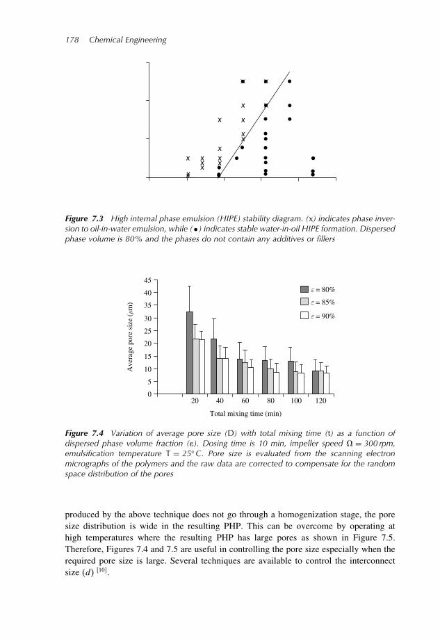
178 Chemical Engineering
Figure 7.3 High internal phase emulsion (HIPE) stability diagram. (x) indicates phase inver-sion to oil-in-water emulsion, while (•) indicates stable water-in-oil HIPE formation. Dispersedphase volume is 80% and the phases do not contain any additives or fillers
Total mixing time (min)
Ave
rage
por
e si
ze (
µm)
0
5
10
15
20
25
30
35
40
45ε = 80%
ε = 85%
ε = 90%
20 40 60 80 100 120
Figure 7.4 Variation of average pore size (D) with total mixing time (t) as a function ofdispersed phase volume fraction (). Dosing time is 10 min, impeller speed = 300 rpm,emulsification temperature T = 25C. Pore size is evaluated from the scanning electronmicrographs of the polymers and the raw data are corrected to compensate for the randomspace distribution of the pores
produced by the above technique does not go through a homogenization stage, the poresize distribution is wide in the resulting PHP. This can be overcome by operating athigh temperatures where the resulting PHP has large pores as shown in Figure 7.5.Therefore, Figures 7.4 and 7.5 are useful in controlling the pore size especially when therequired pore size is large. Several techniques are available to control the interconnectsize (d) 10.

Development of Nano-Structured Micro-Porous Materials 179
0
20
40
60
80
100
120
140
160
0 5 20 60 80
Ave
rage
por
e si
ze, D
(µm
)
Temperature (°C)
10 30 40 50 70
Figure 7.5 Variation of average pore size with emulsification temperature when dosing time=40 s, total mixing time = 100 s, impeller speed = 300 rpm, phase volume = 90%
7.4.5 Effect of Additives/Fillers and Formation of Coalesce Pores
The inclusion of additives in the aqueous phase has several objectives. These additivescan be used to control the pore and interconnect sizes but, most importantly, they canbe used to chemically modify the polymer after polymerization. Surface as well asbulk modification of PHP cannot be achieved through post-polymerization impregnationespecially when the pore/interconnect sizes are small and when the sample is thick.Since the additives are uniformly distributed in the aqueous phase droplets, at the post-polymerization modification stage, the additives are uniformly distributed within thepores. As the aqueous phase is the major emulsion phase, large quantities of desiredsubstances can be incorporated within PHP at levels comparable to that of the polymerphase.The inclusion of oil-soluble fillers in the continuous phase aims to produce co-polymers
or to bulk and/or surface modify the polymer. When the additive does not take partin the polymerization reaction, it can be deemed as ‘filler’ which can then be leachedout to provide nano-porosity to the walls of PHP. Such nano-pores are important intissue engineering and BI since such nano-pores allow the transport of small molecules(nutrients/metabolites) to and from the microorganisms.When the additives/fillers are incorporated in small quantities, stable emulsions are
formed which do not separate or coalesce during polymerization. However, as the con-centration of the additives/fillers are increased, HIPE becomes unstable during polymer-ization, which results in water droplet coalescence leading to larger pores and eventualphase separation if the competing polymerization and cross-linking reactions do not arrestemulsion separation in time. Therefore, the resulting PHP can have very large macro-scopic pores approaching several millimeters. Figure 7.6 illustrates the types of porestructures encountered in PHP. The primary pores in Figure 7.6 (a) and (b) represent

180 Chemical Engineering
(a) (b)
(c) (d)100 µm20 µm
Figure 7.6 Basic polyHIPE polymer structures: (a) primary pores with large interconnectingholes; (b) primary pores with nano-sized interconnecting holes; (c) large coalescence pores(three such pores are partially shown) dispersed into the primary pores in the process ofcoalescence; and (d) detail of the coalescence pores. Note that these pore structures can beprepared over a wide size range
open and close pores, respectively. In the apparently closed-pore PHP, the interconnectsize is very small to be identified at this magnification. By using fillers in the oil phase,it is possible to obtain open-pore PHP with nano-porous pore walls. Figure 7.6 (c) and(d) illustrates the coalescence pores at low and high magnification. The coalescencepores are dispersed into the primary pores which also show signs of coalescence inprogress.The effect of oil-phase additives on average pore size is illustrated in Table 7.1. Here
the additives are water-soluble polymers with varying relative molecular mass. The size ofthe coalescence pores increases with increasing molecular mass as well as concentration.Such polymers are useful in modifying the surface of the hydrophobic polymer for tissueengineering.
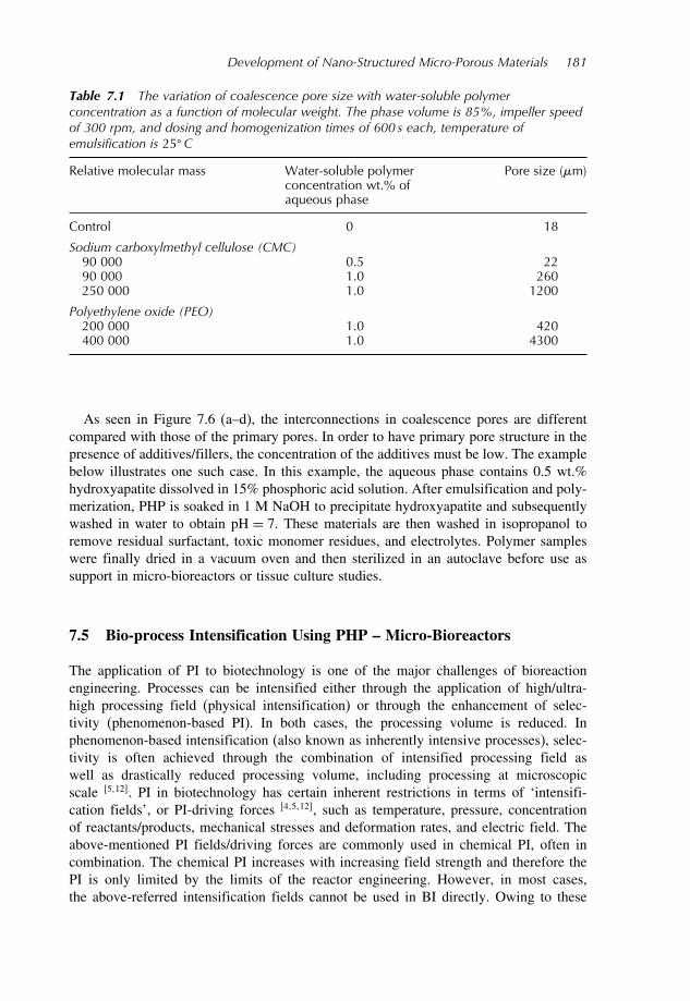
Development of Nano-Structured Micro-Porous Materials 181
Table 7.1 The variation of coalescence pore size with water-soluble polymerconcentration as a function of molecular weight. The phase volume is 85%, impeller speedof 300 rpm, and dosing and homogenization times of 600 s each, temperature ofemulsification is 25C
Relative molecular mass Water-soluble polymerconcentration wt.% ofaqueous phase
Pore size m
Control 0 18
Sodium carboxylmethyl cellulose (CMC)90 000 05 2290 000 10 260250 000 10 1200
Polyethylene oxide (PEO)200 000 10 420400 000 10 4300
As seen in Figure 7.6 (a–d), the interconnections in coalescence pores are differentcompared with those of the primary pores. In order to have primary pore structure in thepresence of additives/fillers, the concentration of the additives must be low. The examplebelow illustrates one such case. In this example, the aqueous phase contains 0.5 wt.%hydroxyapatite dissolved in 15% phosphoric acid solution. After emulsification and poly-merization, PHP is soaked in 1 M NaOH to precipitate hydroxyapatite and subsequentlywashed in water to obtain pH = 7. These materials are then washed in isopropanol toremove residual surfactant, toxic monomer residues, and electrolytes. Polymer sampleswere finally dried in a vacuum oven and then sterilized in an autoclave before use assupport in micro-bioreactors or tissue culture studies.
7.5 Bio-process Intensification Using PHP – Micro-Bioreactors
The application of PI to biotechnology is one of the major challenges of bioreactionengineering. Processes can be intensified either through the application of high/ultra-high processing field (physical intensification) or through the enhancement of selec-tivity (phenomenon-based PI). In both cases, the processing volume is reduced. Inphenomenon-based intensification (also known as inherently intensive processes), selec-tivity is often achieved through the combination of intensified processing field aswell as drastically reduced processing volume, including processing at microscopicscale 512. PI in biotechnology has certain inherent restrictions in terms of ‘intensifi-cation fields’, or PI-driving forces 4512, such as temperature, pressure, concentrationof reactants/products, mechanical stresses and deformation rates, and electric field. Theabove-mentioned PI fields/driving forces are commonly used in chemical PI, often incombination. The chemical PI increases with increasing field strength and therefore thePI is only limited by the limits of the reactor engineering. However, in most cases,the above-referred intensification fields cannot be used in BI directly. Owing to these

182 Chemical Engineering
restrictions on the type of PI-driving forces, BI can therefore be achieved, in the firstinstance, through the reduction of diffusion path for the reactants and products, andthrough the creation of the most suitable environment for the biocatalysts and microorgan-isms which can enhance selectivity thus resulting in phenomenon-based intensification. Itis likely that the optimization of the strength and type of the intensification field will berequired in BI.The most suitable driving force in BI is the reduction in diffusion path which
already operates in transport processes across biological bilayers. Consequently, biocat-alyst membranes and specially designed bioreactors, such as jet loop and membranereactors, are available to intensify biochemical reactions 1235−46. Supported biocata-lysts are often employed in order to enhance catalytic activity and stability, to protectenzymes/microorganisms from mechanical degradation and deactivation123738. Immo-bilization of the cells and enzymes is one of the techniques to improve the productivityfor bioreactors.Immobilized cells are defined as cells that are entrapped within or associated with
an insoluble matrix. Various methods are used for immobilization, including covalentcoupling, adsorption, entrapment in a 3D scaffold, confinement in a liquid–liquid emul-sion, and entrapment within a semi-permeable membrane. Bioreactors with immobilizedcells have several advantages over bioreactors operating with free cells or immobilizedenzymes. Immobilized cell systems permit the operation of bioreactors at flow rates thatare independent of the growth rate of the microorganisms employed. Catalytic stabilitycan be greater for immobilized cells than for free cells. Some immobilized microorgan-isms tolerate higher concentrations of toxic compounds compared with free cells, whenthe cell support media act as a temporary sink for the excess toxin. However, in thecurrent biocatalyst support technology, the presence of the support itself introduces masstransfer restrictions for the substrate/product/nutrient diffusion to and from the biocata-lyst. These disadvantages are also valid when supports are used to grow animal cells invitro10−16.Furthermore, in most cases, the 3D architecture of the support and cell distribution is
also important in cell viability and cell function. The cell support system developed byAkay et al.10 is designed to address these issues. In this study, we use the techniqueof Akay and co-workers810 to obtain micro-cellular polymers of controlled micro-architecture to immobilize bacteria employing a novel seeding technique. Operated asa flow-through system in the degradation of phenol in water, this micro-bioreactor isshown to represent a clear BI.We have chosen phenol for which the metabolic pathways are well described 46−49
as a model substrate to conduct the continuous micro-bioreactor experiments. Thereare various degradation studies using phenol and other aromatic compounds by free orimmobilized microorganisms4649−53. Phenol has a highly toxic effect on all bacteriaand there are various data reported on the inhibition effect of phenol for the growth ofPseudomonas sp. ranging between 50 and 350mg/L54. Furthermore, the degradation ofphenol is aerobic and therefore it presents further challenge to the intensification of bio-conversion. Recently we have also studied the degradation of phenol using immobilizedenzymes4142 and immobilized bacteria1246 using a micro-porous cell support systemoriginally developed for animal cell support for tissue engineering applications 5101115.Phenol degradation studies using immobilized Pseudomonas sp.46 also provide us witha direct base line to compare the BI achieved in the present study.

Development of Nano-Structured Micro-Porous Materials 183
BI was demonstrated by using a well-known bioconversion, namely the degradation ofphenol using Pseudomonas syringae. In the control experiments bacteria was immobilizedon PHP beads and degradation was carried out in a packed bed46. It was found that aftera prolonged operation, biofilm formation on the surface of the support PHP particlesprevented bacterial penetration into the pores of the support. In the case of BI studies,a small PHP disk housed in a sealed reactor was used as the monolithic support. Theexperimental set-up is shown in Figure 7.7 (a), while the detail of the micro-reactor isillustrated in Figure 7.7 (b). Initially, bacteria was force-seeded within the pores andsubsequently allowed to proliferate followed by acclimatization and phenol degradation atvarious initial substrate concentrations and flow rates. Two types of micro-porous polymerwere used as the monolithic support. These polymers differ with respect to their pore andinterconnect sizes, macroscopic surface area for bacterial support, and phase volume. Thepolymer with a nominal pore size of 100 m and with phase volume of 90% (with highlyopen pore structure) yielded reduced bacterial proliferation, while the polymer witha nominal pore size of 25 m and with phase volume of 85% (with small interconnect
Feed tank
Peristalticpump
Micro-bioreactor inlet
Outlet
Waterbath
PHP disk
Micro-bioreactor
Inlet
Outlet
(a)
(b)
Figure 7.7 Micro-bioreactor: (a) flow diagram, and (b) housing detail for the PHP supportfor bacteria or animal cells

184 Chemical Engineering
size and large pore area for bacterial adhesion) yielded monolayer bacterial proliferation.Bacteria within the 25-m polymer support remained monolayered without any apparentproduction of extracellular matrix during the 30-day continuous experimental period. Themonolayer bacterial growth and the lack of extracellular matrix are shown in Figure 7.8.The micro-bioreactor performance was characterized in terms of volumetric utilizationrate and compared with the published data, including the case in which the same bacteriawas immobilized on the surface of micro-porous polymer beads and used in a packedbed during continuous degradation of phenol. The results are summarized in Table 7.2.It is shown that at similar initial substrate concentration, the volumetric utilization in themicro-reactor is at least 20-fold more efficient than the packed bed depending on theflow rate of the substrate solution. The concentration of the bacteria within the poresof the micro-reactor decreases from 2.25 cells per m2 on the top surface to about 0.4cells per m2 within 3-mm reactor depth. The variation of the bacteria concentrationwith distance is shown in Figure 7.9. If the bacteria-depleted part of the micro-reactor isdisregarded, the volumetric utilization increases by a factor of 30-fold compared with thepacked bed. This efficiency increase is attributed to the reduction of diffusion path forthe substrate and nutrients and enhanced availability of the bacteria for bioconversion inthe absence of biofilm formation as well as the presence of flow over the surface of themonolayer bacteria.
Figure 7.8 SEM micrograph of the micro-bioreactor at the end of the 30-day continuouscultivation: cross-section at a distance of 2000m from the inlet surface showing monolayerbacterial coverage and absence of any extracellular matrix

Table
7.2
Com
parison
ofmicro-bioreac
torpe
rforman
cean
dits
compa
rison
with
othe
rsystem
s
Referen
ceQ
(L/h)
Flow
rate
Co(m
g/L)
Initial
substrate
conc
entration
Ug/m
2min
Utilization
rate
R(g/Lh)
Volum
etric
utiliza
tionrate
Rea
ctor
type
FL/m
2min
Flux
rate
Acm
2Rea
ctor
cross-sectiona
larea
H(cm)
Rea
ctor
height
52
Batch
(ben
zene
)13
5–
001
Fibrou
sbe
dBatch
1145
52
Batch
(toluen
e)20
1–
002
Fibrou
sbe
dBatch
1145
42
–50
0078
–Mem
bran
eim
mob
ilize
den
zyme
2.76
(cross-flow
)17
603
46
027
720
843
133
PHP- immob
ilize
dba
cteria
15301
38
46
06
200
554
128
PHP- immob
ilize
dba
cteria
33301
38
46
11
200
103
024
PHP- immob
ilize
dba
cteria
60301
38
41
–46
7009
2–
Mem
bran
e-im
mob
ilize
den
zyme
0.56 (d
ead-en
dflu
x)
453
–
53
1332
39093
024
Three-ph
ase
fluidized
bed
reac
tor
23.80
9326
30
12
012
650
173
3150
Micro-bioreac
tor
5.78
346
05
12
012
380
219
399
Micro-bioreac
tor
5.78
346
05
12
018
380
216
3945
Micro-bioreac
tor
8.67
346
05

186 Chemical Engineering
Distance from the top surface(µm)
Num
ber
of c
ells
(per
100
µ m
2 )
0
50
100
150
200
250
0 1000 2000 3000 4000 5000
Figure 7.9 Variation of bacteria coverage density (number of cells per 100 square m) asa function of distance from the micro-reactor inlet. The intercept of the dashed line indicatesthe optimum thickness of the micro-reactor monolithic support
7.6 PHP Scaffolds for Tissue Engineering
Tissue engineering has the potential to repair/replace damaged/diseased tissue101113−1555. In creating a replacement tissue such as bone or cartilage, it is possible togrow the tissue in vitro initially and transplant it afterwards. In this approach, a porousscaffold that seeds the cells and serves as a template for tissue regeneration is neces-sary. The structure of the biomaterial should meet the criteria of tissue engineering. Itis important to be able to control the scaffold’s spatial arrangement, which in turn con-tributes substantially to its mechanical characteristic limits. The architectural design ofthe scaffold is also important to determine the quantity and shape of the substratum sur-faces available for colonization by in vitro cell seeding. It is also important that the cellscan actively migrate into the scaffold, and that cell attachment occurs by the productionof extracellular matrix proteins. The cells should also retain their phenotype within thescaffold.The tissue engineering approach to bone regeneration is based on the hypothesis that
healthy progenitor cells, either recruited or delivered to an injured site and then undertight regulation, can ultimately regenerate lost or damaged tissue. Recently many cell–polymer constructs are being developed and evaluated for tissue engineering. Polymershave the advantage of being biocompatible, non-toxic, and can be made biodegradableand can also contain micro-channels for the transport of the nutrients and metabolites aswell as for growing nerves for neural excitation 10.
7.7 Cartilage Tissue Engineering
Articular cartilage is composed of cells, chondrocytes, embedded in a resilient matrixof collagen, proteoglycan, and water. There are three main groups of cartilage: hyaline,elastic, and fibrocartilage. Elastic cartilage is found at sites such as the external ear andepiglottis. Fibrocartilage has a matrix with type I collagen fibers and is located at the

Development of Nano-Structured Micro-Porous Materials 187
pubic symphysis and many tendon insertions into bone. Hyaline cartilage contains type IIcollagen fibers in its matrix and is found in the nasal and respiratory tract and at mostsynovial joints (articular cartilage). It is articular or hyaline cartilage which we considerhere. An important feature of hyaline is the production of collagen II as opposed tocollagen I. The chondrocytes that were used in this study were primary cells obtainedfrom a bovine metacarpalphalangeal joint.Chondrocytes were seeded onto the two types of polymer. The first polymer was a
plain styrene/2EHA PHP which had not been chemically modified. The second PHP(HA-PHP) had been chemically modified to include a coating of hydroxyapatite. Hydrox-yapatite is a mineral found in large quantities in bone and other tissues. Details of thetechnique are found in Ref.56. Primary cells were seeded onto the PHP support and theywere cultured for various time spans. These polymer/cell constructs were then examinedthrough histology or SEM to determine the penetration of the cells and their morphologyas a function of time. The penetration of the chondrocytes into the polymer was deter-mined by histology. The production of glycosaminoglycans (GAG) which are found inthe extracellular matrix was determined by a colorimetric assay and the type of collagenproduced in the matrix was determined with immunocytochemistry. This matrix (GAG)gives cartilage its load-bearing capacity and is crucial to the development of chondro-cytes into cartilage tissue. As seen from the SEM micrograph in Figure 7.10, roundedmorphology of the chondrocytes are preserved within the pores of the hydroxyapatite-coated PHP. The DNA concentration obtained from the chondrocytes/polymer constructsis used to quantify the cell growth rate. It was found that the cell growth rate could bethreefold higher in hydroxyapatite-coated PHP supports compared with non-coated PHPafter 10 days in culture.In order to test the effect of pore size on the cell penetration and collogen II production
rates, five types of styrene/2EHA PHP were produced with average pore sizes D of8, 17, 24, 31, 45, and 89m. The corresponding average interconnect sizes d in these
Figure 7.10 SEM micrograph showing the rounded morphology of chondrocytes on thesurface pores of HA-PHP

188 Chemical Engineering
polymers were 2.5, 5, 6, 6, 7, and 7m, respectively, so as to eliminate the effect ofinterconnect size in the experiments. These samples were then seeded with chondrocytesand the effects of pore size on cell penetration and GAG production rate were determinedafter 21 days in culture. The results are shown in Figures 7.11 and 7.12. As seen inFigure 7.11, maximum cell penetration occurs when D = 24m and d = 6m, andcontrary to the expectations, larger pore and interconnect size PHPs do not facilitatecell penetration. Similarly, GAG production is maximum when the 24-m polymer is
0
100
200
300
400
500
600
Pore size, D (µm)
Dep
th o
f pe
netr
atio
n (µ
m)
8 17 24 31 45 89
Figure 7.11 Effect of pore size on the depth of penetration of chondrocytes, measuredfrom histological sections of chondrocytes on various pore-sized hydroxylapatite-coated2EHA/styrene (copolymer) polyHIPE polymer after 21 days in culture. Each bar representsthe mean ± SE for eight samples with six sections being taken from each sample
0
200
400
600
800
GA
G p
rodu
ctio
n at
day
21
(µg/
mL
)
Pore size, D (µm)
8 17 24 31 45 89
Figure 7.12 Effect of pore size on the production of total glycosaminoglycan (GAG) protein(cell associated + released into the medium) by chondrocytes cultured on various pore-sizedhydroxylapatite-coated 2EHA/styrene (copolymer) polyHIPE polymer after 21 days in culture

Development of Nano-Structured Micro-Porous Materials 189
used. These experiments were also conducted using tissue culture plastic (TCP) whichis non-porous but coated with bioactive proteins to enhance cell growth. TCP-grownchondrocytes yielded GAG production levels similar to those observed for the 89-mpolymer. However, at longer time spans, chondrocytes on TCP become flattened. Theseresults indicate that there is an optimum pore size to maintain the chondrocyte morphologyand to optimize the production of collagen II. At lower pore sizes, the cells cannotpenetrate the polymer and at higher pore sizes the cells’ morphology changes fromrounded to flat and fibroblastic in appearance. These fibroblastic cells proliferate rapidlyand form a layer on the surface rather than penetrating the polymer.
7.8 Bone Tissue Engineering
The experimental technique in the study of bone tissue engineering is similar to thatof the cartilage tissue engineering described earlier. However, in order to acceleratethe cell penetration into the PHP, we employed a forced seeding technique which wasalso employed in the seeding of the bacteria into the micro-bioreactor as shown inFigure 7.7 (b). In these studies, we used styrene only in the support system in order toenhance and match the mechanical properties of the support with that of the bone. Porevolume fraction was 95%. Three different pore sizes were used: 40, 60, and 100 m.However, in this case the corresponding interconnect sizes were 15, 20, and 30 m,respectively. Once again, some of the samples were coated with hydroxapatite with anestimated coating thickness ranging from 25 nm for the 40-m pore material to 40 nmfor the 100-m pore size PHP 11155556.
Statically seeded disks were cultured for periods between 7 and 35 days on PHP andsubsequently prepared for analysis. SEM was used to examine cell morphology on thepolymer surface and inside of the polymers. SEM analysis (Figure 7.13) shows surfaceand transverse sections seeded with primary rat osteoblasts and demonstrates that thecells reached confluence on the surface after 14 days (Figure 7.13 (a)) and formed acontinuous, thick layer that at later time points became multilayered sheets, with fibrousmatrix present (Figure 7.13 (b)). Osteoblasts were also observed within the polymers(Figure 7.13 (c)), but these were fewer in number and were present as either individualcells or in isolated colonies.The effect of including hydroxyapatite during the preparation of PHP was further
investigated by comparing its performance with the unmodified polymers. In these exper-iments rat osteoblasts were seeded onto the surface of 40-, 60-, and 100-m pore sizepolymers that were either unmodified or modified with hydroxyapatite and cell growthand migration assessed by histological analysis.The amount of bone nodule formation was quantified from the surfaces of unmodified
and modified polymers at 28 and 35 days in culture under osteogenic conditions, for eachof the three different pore-sized polymers. Histomorphometric analysis shows that thesurfaces of modified polymers had significantly increased areas of Von Kossa staining(Figure 7.14) compared to unmodified polymers. Increased amounts of nodule formationcan be observed for each of the different pore sizes between days 28 and 35 but thisis only significant for 100-m pore size. There was no evidence that nodule area wassignificantly influenced by the three pore sizes evaluated in this study.Image analysis reveals that when polymers are modified with hydroxyapatite there is a
significant increase in the penetration of cells into the polymer compared to unmodified

190 Chemical Engineering
(a)
(c)
(b)
Figure 7.13 Scanning electron micrographs of primary rat osteoblasts cultured inhydroxylapatite-coated PHP. (a) Surface appearance after 14 days; (b) surface appearanceafter 35 days; and (c) transverse section after 35 days illustrating the penetration of boneformation
controls that were independent of pore size. Relatively few cells penetrated deeper than1mm in any of the PHPs tested, regardless of pore size. Between the different pore sizesevaluated, significantly more cells could be found beneath the surface of 40-m modifiedPHP compared to both 60- and 100-m modified PHPs.There was little overall effect of pore size on the maximal depth of cell penetration
into the polymer at 35 days (approximately 1.4 mm). Cell movement into all the PHPstested progressed with time, but the rate was notably quicker with the 100-m pore sizepolymer in comparison to the 40- and 60-m pore size polymers.The effect of pore size on cell concentration in the polyHIPE support at different times
was determined from DNA analysis of the cell/polymer constructs. The results are shownin Figure 7.15 which indicates that DNA content per construct increases with increasingpore size. Since the pore size span in the experiments is not large (2.5-fold) the differencesbetween the DNA contents are not as marked as the case for chondrocytes where the poresize span was 10-fold. Nevertheless, the present results also indicate that for a given celltype, an optimum pore size is present for cell proliferation as indicated by DNA content in

Development of Nano-Structured Micro-Porous Materials 191
Pore size (µm)
4.5
4.0
3.5
3.0
2.5
2.0
1.5
1.0
0.5
0.0
Tot
al a
rea
of n
odul
e fo
rmat
ion
per
PHP
surf
ace
(mm
2 )35 days28 days
100
Modified
Unmodified
100 60 40 60100 40
*
*
*
*
**
Figure 7.14 Effect of support pore size (D=100, 60, 40 m) on mineralized nodule forma-tion of rat osteoblast cells cultured in vitro after 28 or 35 days using hydroxylapatite-coated(modified) or uncoated (unmodified) styrene PolyHIPE Polymer cell supports
DN
A c
once
ntra
tion
(µg/
scaf
fold
)
0
5000
10000
15000
20000
PHP 100 PHP 60 PHP 40
7 days
14 days
28 days
35 days
Figure 7.15 Effect of pore size on DNA concentration as a function of time in cultureof rat osteoblast cells in hydroxyapatite-coated polyHIPE polymer support, illustrating thedependence of cell proliferation rate on support pore size

192 Chemical Engineering
the supports. The results also indicate that the coating of the polymers with hydroxyapatiteincreases cell penetration, and proliferation and further enhancement is possible whenthe hydroxyapatite-coated PHPs are coated with self-assembling peptide hydrogel1557.
7.9 Nano-Structured Micro-Porous Metalsfor Intensified Catalysis
Surface area and its accessibility are important both in catalysis and gas cleanup. Nano-structured micro-porous catalysts or catalyst supports offer intensified catalysis sincethey provide an enhanced surface area which is accessible to the reactants and productsthrough a network of arterial channels feeding into the regions of catalytic activity. Innon-structured catalysts, although the surface area might be large, as determined by gasadsorption, they are often not accessible as a result of surface fouling and the diffusionresistance can slow down the rates of reactions. Catalysts are either deposited as athin film on a support or they are used as pellets. These two techniques have certaindrawbacks: in coated systems, catalyst adhesion can be non-uniform and weak while theaccessibility of the active sites within the interior of the catalyst is hindered due to lowporosity.In this study we summarize the recent developments in catalyst development in which
nano-porous catalytic sites are accessible through a network of arterial micro-pores.These catalysts are obtained through a solution deposition of metals on a micro-porouspolymeric template which is subsequently heat-treated to obtain porous metallic structureswhere the size of the pores ranged from tens of micrometers to tens of nanometersthus eliminating the problems of accessibility and rapid pore fouling and closure. Thetechnique differs fundamentally from the compression-based systems where the porosityis reduced as a result of compaction. It also differs from the well-known wash-coating orchemical vapor deposition techniques. Furthermore, the mechanisms of metal depositionwithin micro-pores and nano-structure formation are novel. The importance and currentfabrication techniques of porous metallic systems can be found in Refs.516.
Figure 7.16 illustrates the micro-structure of these novel materials. The overall skeleton(Figure 7.16a) is formed by fused metallic (nickel alloy) grains of ca. 8m formingmicro-pores of ca. 30-m arterial passages (channels). As seen in Figure 7.16 (a), grainsthemselves are porous which can be clearly identified in Figure 7.16 (b) from where thesize of the surface pores can be evaluated to be ca. 200 nm. However, further detailedexamination reveals that these materials have finer structures well below 100 nm as seenin Figure 7.16 (c). All of these parameters – grain, arterial channel – and grain poresizes – can be controlled. As the grains themselves are porous, they provide a largeavailable surface area. Details of material preparation are available16. These materialsare based on nickel which is useful as a catalyst in many gas phase reactions.
7.10 Concluding Remarks
This paper summarizes the recent developments in micro-fabrication and its applica-tions in PI and tissue engineering which is complementary to phenomenon-based BI.In such intensified processes, miniaturization is essential and therefore micro-reactors

Development of Nano-Structured Micro-Porous Materials 193
Figure 7.16 Micro-structure of nickel-based intensified catalyst/catalyst support showing thehierarchy of the pore sizes: (a) arterial micro-pores; (b) nano-structure of the surface poresof the fused metallic grains; and (c) nano-structure of the inside of the fused metal grainsshowing even smaller pore structure than the surface pores

194 Chemical Engineering
with stagewise processes in micro-scale represent a novel processing approach. Suchmicro-reactors/unit-operations are already available in nature, in the form of organswhere micro-channels and neural network between the collection of cells provide thenecessary facilities for the organ function. In these systems, diffusion takes place acrossnano-scale lipid bilayers. Such miniaturized systems can be achieved in vitro by usingmicro-porous materials with a network of capillaries having nano-porous walls separatingdifferent domains. Monolithic PHPs with a network of capillaries have been proposed10
to mimic the micro-architecture of organs. Metallic versions of such micro-reactors arealso described in this study.We have also provided evidence that the behavior of microorganisms in confined
micro-environment is substantially different and that their desired metabolic activitiescan be maximized through the modification of the surface characteristics as well as thesize of the pores. These characteristics can therefore be utilized in BI as well as in theenhancement of cell penetration and cell proliferation in tissue engineering and when suchpolymers are grafted. Micro-fabrication technique has also been used in the developmentof highly porous catalysts with arterial channels feeding nano-pores which provide anextended surface area. Such materials can be used as micro-reactors as well as catalysts.
Acknowledgements
We are grateful to the UK Engineering and Physical Sciences Research Council (EPSRC),UK Department of Trade and Industry, Avecia/Cytec, BLC Research, BP Amoco, Exxon,Intensified Technologies Incorporated (ITI), Morecroft Engineers Ltd., Safety-KleenEurope, Triton Chemical Systems, andWillacy Oil Services Ltd. for their support. We alsothank Burak Calkan, Omer Calkan, and Zainora Noor for their help in the experiments.
References
[1] Akay G. 1986. Rheological properties of thermoplastics. In, Encyclopedia of Fluid Mechanics,Cheremisinoff N.P.(Ed.), Vol. 1, Chapter 35, Gulf Publishing, Houston, USA pp. 1155–1204.
[2] Agarwal U.S., Dutta A. and Mashelkar R.A. 1994. Migration of macromolecules under flow:The physical origin and engineering implications, Chem. Eng. Sci., 49, 1693–1717.
[3] Akay G. 1998. Flow-induced phase inversion in the intensive processing of concentratedemulsions, Chem. Eng. Sci., 53, 203–223.
[4] Akay G., Mackley M.R., Ramshaw C. 1997. Process intensification: Opportunities for processand product innovation. In, IChemE Research Event, Chameleon Press, London, pp. 597–606.
[5] Akay G. 2005. Bioprocess and Chemical Process Intensification. In, Encyclopaedia of Chem-ical Processing, Lee S. (Ed.), Marcel Dekker, NY.
[6] Akay G., Wakeman R.J. 1994. Mechanism of permeate flux decay, solute rejection andconcentration polarisation in crossflow filtration of a double chain ionic surfactant dispersion,J. Membr. Sci., 88, 177–195.
[7] Akay G., Odirile P.T., Keskinler B., Wakeman R.J. 2000. Crossflow microfiltration character-istics of surfactants: The effects of membrane physical chemistry and surfactant phase behavioron gel polarization and rejection. In, Surfactant Based Separations: Science and Technology,Scamehorn J.F. and Harwell J.H. (Eds.), ACS Symposium Series, 740, 175–200.

Development of Nano-Structured Micro-Porous Materials 195
[8] Akay G., Vickers J. 2003. Method for separating oil in water emulsions, European Patent,EP 1 307 402.
[9] Akay G., Noor Z.Z., Dogru M. 2005. Process intensification in water-in-crude oil emulsionseparation by simultaneous application of electric field and novel demulsifier adsorbers.In, Microreactor Technology and Process Intensification, Wang Y. and Halladay J. (Eds.),Chapter 23, ACS Symposium Series, Oxford University Press, Oxford.
[10] Akay G., Dawnes S., Price V.J. 2002. Microcellular polymers as cell growth media and novelpolymers, European Patent, EP 1 183 328.
[11] Akay G., Birch M.A., Bokhari M.A. 2004. Microcellular Polyhipe polymer (PHP) supportsosteoblastic growth and bone formation in vitro, Biomaterials, 25, 3991–4000.
[12] Akay G., Erhan E. and Keskinler B. 2005. Bioprocess intensification in flow through micro-reactors with immobilized bacteria, Biotechnol. Bioeng., 90, 180–190 (in press). Publishedon line, 1 March 2005.
[13] Yang S., Leong K-F., Du Z. and Chua C-K. 2001. The design of scaffolds in tissue engi-neering. Part 1. Traditional factors, Tissue Eng., 7, 679–689.
[14] Zhang S. 2003. Fabrication of novel biomaterials through molecular self assembly, Nat.Biotechnol., 21, 1171–1178.
[15] Bokhari M.A., Akay G., Birch M.A., Zhang S. 2005. The enhancement of osteoblast growthand differentiation in vitro on a peptide hydrogel – PolyHIPE Polymer hybrid supportmaterial. Biomaterials, 26, 5198–5208 (in press).
[16] Akay G., Dogru M., Calkan B. and Calkan O.F. 2005. Flow induced phase inversion phe-nomenon in process intensification and micro-reactor technology. In, Microreactor Technol-ogy and Process Intensification, Wang Y. and Halladay J.(Eds.), Chapter 18, ACS SymposiumSeries, Oxford University Press, Oxford.
[17] Stankiewicz A., Moulijn J.A. 2002. Process intensification, Ind. Eng. Chem. Res., 41, 1920–1924.
[18] Stankiewicz A., Drinkenburg A.A.H. 2004. Process intensification: History, philosophy,principles. In, Chemical Industries, Marcel Dekker, NY pp. 1–32.
[19] Akay G. 1991. Agglomerated abrasive material compositions comprising same, and processfor its manufacture, US Patent, US 4 988 369.
[20] Akay G. 1995. Flow-induced phase inversion in powder structuring by polymers. In, PolymerPowder Technology, Narkis M. and Rosenzweig N.(Eds.), Chapter 20, Wiley pp. 542–587.
[21] Akay G. 2001. Stable oil in water emulsions and a process for preparing same, EuropeanPatent, EP 649 867.
[22] Akay G., Tong L., Addleman R. 2002. Process intensification in particle technology: Intensivegranulation of powders by thermo-mechanically induced melt fracture, Ind. Eng. Chem. Res.,41, 5436–5446.
[23] Akay G., Tong L. 2003. Process intensification in particle technology: Intensive agglomer-ation and microencapsulation of powders by non-isothermal flow induced phase inversionprocess, Int. J. Transp. Phenomena, 5, 227–245.
[24] Akay G., Tong L. 2003. Process intensification in polymer particle technology: Granulationmechanism and granule characteristics J. Mater. Sci., 38, 3169–3181.
[25] Akay G. 2004. Upping the ante in the process stakes, Chem. Eng., 752, 37–39.[26] Akay G. 2004. International Patent Application, Method and apparatus for processing flow-
able materials and microporous polymers, WO 2004/004880.[27] Akay G., Tong L. 2001. Preparation of low-density polyethylene latexes by flow-induced
phase inversion emulsification of polymer melt in water, J. Colloid Interface Sci., 239,342–357.
[28] Akay G., Tong L., Hounslow M.J., Burbidge A. 2001. Intensive agglomeration and microen-capsulation of powders, Colloid Polym. Sci., 279, 1118–1125.
[29] Akay G., Irving G.N., Kowalski A.J., Machin D. 2001. Process for the production of liquidcompositions, European Patent, EP 799303.

196 Chemical Engineering
[30] Tong L., Akay G. 2002. Process intensification in particle technology: Flow induced phaseinversion in the intensive emulsification of polymer melts in water, J. Mater. Sci., 37, 4985–4992.
[31] Akay G., Tong L., Bakr H., Choudhery R.A., Murray K., Watkins J. 2002. Preparationof ethylene vinyl acetate copolymer latex by flow induced phase inversion emulsification,J. Mater. Sci., 37, 4811–4818.
[32] Akay G. 2004. International Patent Application, Microporous polymers, WO 2004/005355.[33] Akay G. 2000. Flow induced phase inversion. In, Recent Advances in Transport Phenomena,
Dincer I. and Yardim F. (Eds.), Elsevier, Paris pp. 11–17.[34] Akay G., Irving G.N., Kowalski A.J., Machin D. 2002. Dynamic mixing apparatus for the
production of liquid compositions, US Patent, US 63445907.[35] Chisti Y., Moo-Young M. 1996. Bioprocess intensification through bioreactor engineering,
Trans. IChemE, 74, 575–581.[36] Giorno L., Drioli E. 2000. Biocatalyst membrane reactors: Applications and perspectives,
TIBTECH, 18, 339–349.[37] De Bartolo L., Morelli A., Bader D., Drioli E. 2001. The influence of polymeric membrane
surface free energy on cell metabolic functions, J. Mater. Sci., Materials in Medicine, 12,959–963.
[38] Bayhan Y.K., Keskinler B., Cakici A., Levent M., Akay G. 2001. Removal of divalent heavymetal mixtures from water by Saccharomyces cerevisiae using crossflow microfiltration,Water Res., 35, 2191–2200.
[39] Nuhoglu A., Pekdemir T., Yildiz E., Keskinler B., Akay G. 2002. Drinking water denitrifi-cation by a membrane bioreactor, Water Res., 36, 1155–1166.
[40] Erhan E., Keskinler B., Akay G., Algur O.F. 2002. Removal of phenol from wastewaterby using membrane immobilized enzymes: Part 1. Dead end filtration, J. Memb. Sci., 206,361–373.
[41] Akay G., Erhan E., Keskinler B., Algur O.F. 2002. Removal of phenol from wastewaterby using membrane-immobilized enzymes: Part 2. Crossflow filtration, J. Memb. Sci., 206,61–68.
[42] Pekdemir T., Keskinler B., Yildiz E., Akay G. 2003. Process intensification in wastewatertreatment: ferrous iron removal by a sustainable membrane bioreactor system, J. Chem.Technol. Biotechnol., 78, 773–780.
[43] Yildiz E., Keskinler B., Pekdemir T., Akay G., Nihoglu A. 2005. High strength wastewatertreatment in a jet loop membrane bioreactor: Kinetics and performance evaluation, Chem.Eng. Sci., 60, 1103–1116.
[44] Keskinler B., Yildiz E., Erhan E., Dogru M., Akay G. 2004. Crossflow microfiltration oflow concentration- non-living yeast suspensions, J. Memb. Sci., 233, 59–69.
[45] Keskinler B., Akay G., Pekdemir T., Yildiz E., Nuhoglu A. 2004. Process intensificationin wastewater treatment: Oxygen transfer characteristics of a jet loop reactor for aerobicbiological wastewater treatment. Int. J. Environ. Technol. Manag., 4, 220–235.
[46] Erhan E., Yer E., Akay G., Keskinler B., Keskinler D. 2004. Phenol degradation in a fixedbed bioreactor using micro-cellular polymer-immobilized Pseudomonas syringae, J. Chem.Technol. Biotechnol., 79, 196–206.
[47] Dagley S. 1971. Catabolism of aromatic compounds by microorganisms. Adv. Microbial.Physiol., 6, 1–46.
[48] Buswell J.A. 1975. Metabolism of phenol and cresols by Bacillus stearothermophilusJ. Bacteriol., 124, 1077–1083.
[49] Kline J., Schara P. 1981. Entrapment of living microbial cells in covalent polymeric networks.II. A quantitative study on the kinetics of oxidative phenol degradation by entrapped andidatropicalis cells, Appl. Biochem. Biotechnol., 6, 91–117.
[50] Bettmann H., Rehm H.J. 1984. Degradation of phenol by polymer entrapped microorganisms,Appl. Microbiol. Biotechnol., 20, 285–290.

Development of Nano-Structured Micro-Porous Materials 197
[51] Schröder M., Muller C., Posten C., Deckwer W.D., Hecht V. 1996. Inhibition kinetics ofphenol degradation from unstable steady-state data, Biotechnol. Bioeng., 54, 567–576.
[52] Shim H., Yang S.T. 1999. Biodegradation of benzene, toluene. Ethylbenzene, and o-xyleneby a coculture of Pseudomonas putida and Pseudomonas fluorescens immobilized in afibrous-bed bioreactor, J. Biotechnol., 67, 99–112
[53] Hecht V., Langer O., Deckwer W.D. 2000. Degradation of phenol and benzoic acid in athree-phase fluidized bed-reactor, Biotechnol. Bioeng., 70, 391–399.
[54] Hill G.A., Robinson C.W. 1975. Substrate inhibition kinetics: Phenol degradation byPseudomonas putida, Biotechnol. Bioeng., 17, 1599–1615.
[55] Bokhari M., Birch M., Akay G. 2003. Polyhipe polymer: A novel scaffold for in vitrobone tissue engineering, Adv. Exp. Med. Biol. (Tissue Engineering, Stem Cells, and GeneTherapies), 534, 247–254.
[56] Byron V.J. 2000. The development of microcellular polymers as support for tissue engineer-ing, PhD Thesis, University of Newcastle, Newcastle upon Tyne, UK.
[57] Bokhari M.A. 2003. Bone tissue engineering using novel microcellular polymers, PhD Thesis,University of Newcastle, Newcastle upon Tyne, UK.

8The Encapsulation Art: Scale-up and
Applications
M.A. Galán, C.A. Ruiz and E.M. Del Valle
8.1 Control Release Technology and Microencapsulation
Controlled release technologies are invaluable scientific tools for improving the per-formance and safety of chemicals. They involve materials such as barriers surroundingactive materials to deliver the latter at the optimum time and rate needed12.
The technical objective of this science is to find and use judiciously barriers, usuallyspecially designed polymers (but may include adsorption inorganics or complexing withcertain chemicals). Such formulations have also provided drug manufacturers, in partic-ular, with a method for the measured, slow release of drugs as well as a business tacticfor extending patent life and usefully differentiating their product. Methods include thefollowing12:
• Designing the barrier surrounding the active chemical so as to change its permeabilityfor the extraction and thus provide a tortuous path. Means include designing the barriermaterial to swell or slowly dissolve in the extracting fluid.
• Selection of an inorganic material which will adsorb the active material within itslayered or porous structure, thus again providing a torturous path for the extractingfluid.
• Designing a chemical which will complex the active material and release it at acontrolled rate under the right environmental conditions.
• Controlling the chemistry of the active material itself to release only under certainenvironmental conditions.
The application may require release in different ways: (a) constant release over time;(b) release rate diminishing with time; and (c) ‘burst release’, where all of the active
Chemical Engineering: Trends and Developments. Edited by Miguel A. Galán and Eva Martin del ValleCopyright 2005 John Wiley & Sons, Inc., ISBN 0-470-02498-4 (HB)
200 Chemical Engineering
material is released suddenly at a particular time, such as after the drug has passedthrough the stomach into the intestines. Designing the barrier makes use of the dissolvingrates or swelling rates of the barrier polymer. In turn, the dissolving or swelling ratesand permeability may depend on the pH, moisture, and temperature of the environment,chemical properties of the encapsulating polymer, its size, shape, and thickness.Microencapsulation is an important sub-category of controlled release technology.
Active materials are encapsulated in micrometer-sized capsules of barrier polymersdesigned to control the rate of release of the active materials that are encapsulated. Theterm ‘microencapsulation’ is often confused with ‘controlled release’ but the latter ismuch more inclusive, as indicated above13.
8.2 The Microcapsule
In its simplest form, a microcapsule consists of a small ball surrounded by a homogeneouscoating. The material enclosed in the microcapsule is called4:
• Core, or nucleus, internal phase, encapsulated, active substance, etc.
The coating is also called:
• Shell, envelope, external phase, membrane.
Although this is the most common type, there are several other kinds of microcapsules,depending on the technology used in their production. Their size usually varies from1 to 2000m.Capsules smaller than 1m are called nano-capsules because their size is measured in
nanometers. When the core and the coating are not really separated, the microcapsule, ornanocapsule, is called microparticle, or nanoparticle.The architecture of microcapsules is generally divided into several arbitrary and over-
lapping classifications. One such design is known as matrix encapsulation. Where thematrix particle resembles that of a peanut cluster. The core material is buried to varyingdepths inside the wall material. The most common type of microcapsule is that of aspherical or reservoir design. It is this design that resembles a hen’s egg. It is also pos-sible to design microcapsules that have multiple cores which may be an agglomerate ofseveral different types of microcapsules135. If the core material is an irregular material,such as occurs with a ground particle, then the wall will somewhat follow the contourof the irregular particle and one achieves an irregular microcapsule. The last well-knowndesign for a microcapsule is that of a multiple wall. In this case, multiple walls are placedaround a core to achieve multiple purposes related to the manufacture of the capsules,their subsequent storage and controlled release.
8.2.1 Properties of the Core and the Capsule
The core, which is the substance to microencapsulate, can have different characteristics.It may belong to various categories of chemical substances. It can be liquid or solid,

The Encapsulation Art: Scale-up and Applications 201
acid or basic, in powder or rough crystals. In addition to the requirement to inducemicroencapsulation of certain substances, the choice of the microencapsulation methodand the coating material also depends on the characteristics of the active principle67.
The choice of the coating material (capsule) often depends on the purpose, or thepurposes, of microencapsulation. Not all membranes are able to confer specific propertiesonto the microencapsulated product. The choice of the right coating is often crucial inachieving the microencapsulation purpose. Some one hundred suitable substances havebeen described (and already used) to form a microcapsule film. The most commonlyused substances are collected in Table 8.1.Therefore, the first process consists of forming a wall around the core material. The
second process involves keeping the core inside the wall material so that it does notrelease. Also, the wall material must prevent the entrance of undesirable materials thatmay harm the core. And finally, it is necessary to release the core material at the righttime and at the right rate.Microencapsulation is like the work of a clothing designer. He selects the pattern,
cuts the cloth, and sews the garment in due consideration of the desires and age of hiscustomer, plus the locale and climate where the garment is to be worn. By analogy, inmicroencapsulation, capsules are designed and prepared to meet all the requirements indue consideration of the properties of the core material, intended use of the product, andthe environment of storage.In a discussion of microencapsulation technology, particularly when one is talking
about quantities and cost, it is necessary to understand that encapsulation is a volumeprocess, independent of the density or value of the core material. Thus, microencapsulatorsfrequently state that it is just as expensive on a volume basis to encapsulate diamond asgraphite. Likewise, on a volume basis it is just as expensive to encapsulate paraffin waxas tungsten metal. Also, when experimenting with or acquiring microcapsules, it shouldbe emphasized that it is necessary to use common, consistant terminology because of thepreference for discussing microcapsules in terms of the core material, particularly whenone is discussing the cost of production7−9.
8.2.2 Microcapsules Uses
The uses of microcapsules since the initial coacervation work in the 1940s are manyand varied. A good early review of these uses that also includes pharmaceuticals and
Table 8.1 Materials used as coating material
• Agar • Albumin• Cellulose and its derivatives • Gelatin• Arabic gum • Hydrogenated fats• Glutens • Glycerides• Polyamides • Acrylic polymers• Polyesters • Polyvinyl pyrrolidone• Polyethylene glycols • Polystyrene• Starch • Stearic acid• Paraffins • Waxes• Polyvinyl, myristic, stearyl alcohols, etc. • Others

202 Chemical Engineering
agricultural materials is provided by Gutcho6. The uses of microcapsules that are ofinterest here include the following10:
1. Reduce the reactivity of the core with regard to the outside environment, for exampleoxygen and water.
2. Decrease the evaporation or transfer rate of the core material with regard to the outsideenvironment.
3. Promote the ease of handling of the core material:
a. prevent lumping;b. position the core material more uniformly through a mix by giving it a size and
outside surface matching the remainder of the materials in the mix;c. convert a liquid to a solid form; andd. promote the easy mixing of the core material.
4. Control the release of the core material so as to achieve the proper delay until theright stimulus.
5. Mask the taste of the core.6. Dilute the core material when it is only used in very small amounts; but, achieve
uniform dispersion in the host material.
8.2.3 Release Mechanisms
A variety of release mechanisms have been proposed for microcapsules; but, in fact,those that have actually been achieved and are of interest here are rather limited. Theseare as follows:
1. A compressive force in terms of a 2 point or a 12 point force breaks open the capsuleby mechanical means.
2. The capsule is broken open in a shear mode such as that in a Waring blender or aZ-blade type mixer.
3. The wall is dissolved away from around the core such as when a liquid flavoring oilis used in a dry powdered beverage mix.
4. The wall melts away from the core releasing the core in an environment such as thatoccurring during baking.
5. The core diffuses through the wall at a slow rate due to the influence of an exteriorfluid such as water or by an elevated temperature1−4.
8.2.4 Release Rates
The release rates that are achievable from a single microcapsule are generally ‘0’ order,1/2 order, or 1st order. ‘0’ order occurs when the core is a pure material and releasesthrough the wall of a reservoir microcapsule as a pure material. The 1/2-order releasegenerally occurs with matrix particles. 1st-order release occurs when the core material isactually a solution. As the solute material releases from the capsule the concentration ofsolute material in the solvent decreases and a 1st-order release is achieved. Please notethat these types of release rates occur from a given single microcapsule. A mixture ofmicrocapsules will include a distribution of capsules varying in size and wall thickness.The effect, therefore, is to produce a release rate different from ‘0’, ‘1/2’, or ‘1’ becauseof the ensemble of microcapsules. It is therefore very desirable to examine carefully on

The Encapsulation Art: Scale-up and Applications 203
an experimental basis the release rate from a collection of microcapsules and to recognizethat the deviation from theory is due to the distribution in size and wall thickness911.
8.2.5 Microcapsule Formation
The general technology for forming microcapsules is divided into two classificationsknown as physical methods and chemical methods. The physical methods are generallydivided into the following1−356:
Spray coating
Pan coating: This is a mature, well-established technology initially patented by apharmacist in the 19th century by the name of Upjohn. Generally, it requires largecore particles and produces the coated tablets that we are familiar with.Fluid bed coating: One version of this coating is known as Wurster coating and wasdeveloped in the 1950s and 1960s. The Wurster coater relies upon a bottom-positionednozzle spraying the wall material up into a fluidized bed of core particles. Anotherversion sprays the wall material down into the core particles.
Annular jet. This technology was developed by the Southwest Research Institute andhas not been extensively used in the food industry. It relies upon two concentric jets. Theinner jet contains the liquid core material. The outer jet contains the liquid wall material,generally molten, that solidifies upon exiting the jet. This dual fluid stream breaks intodroplets much as water does upon exiting a spray nozzle.
Spinning disk. A new method was developed by Professor Robert E. Sparks atWashington University in St Louis. This method relies upon a spinning disk and thesimultaneous motion of core material and wall material exiting from that disk in dropletform. The capsules and particles of wall material are collected below the disk. Thecapsules are separated from the wall particles (chaff) by a sizing operation.
Spray cooling. This is a method of spray cooling a molten matrix material containingminute droplets of the core materials. This method is practiced by the Sunkist Company.
Spray drying. Spray dryers can be used from small to very high productions dependingon their design. They can reach evaporative capacities of up to 15 000 lb/h. Even thoughthe cost of the equipment is expensive, the cost of maintenance is low due to the smallnumber of moving parts and the use of resistant materials. The purity of the productwill be maintained since the food particles do not have any contact with the surface ofthe equipment until they are dried, minimizing problems in sticking and corrosion. Thesimple operating system and the cleaning conditions for spray dryers contribute to thelow labor cost. Another advantage of using the spray drying method is that a low bulkdensity of the product can be obtained.
Spray chilling. This is a process of spray chilling the wall around an atomized core. Theresulting capsules move countercurrent to a flow of tempered air and are collected in alarge container below the spray nozzle. It is practiced currently by the Durkee Company.

204 Chemical Engineering
Co-extrusion processes. Liquid core and shell materials are pumped through concentricorifices, with the core material flowing in the central orifice, and the shell materialflowing through the outer annulus. A compound drop forms that is composed of a dropletof core fluid encased in a layer of shell fluid.The centrifugal nozzle technique was developed by SwRI. It requires that, initially,
both the core and the wall are pumpable liquids (or thin slurries). Both fluids are fedinto a special nozzle so that a coaxial stream is formed at the nozzle. This nozzle isspun rapidly, which stretches out the liquid ligaments and breaks off individual droplets.Surface tension pull the ‘shell’ material around the core droplet to form a completecovering. The wall material must be selected so that it will solidify before the particle iscollected.
Use of supercritical fluids. Supercritical fluid (SCF) technology is now considered asa very innovative and promising way to design particles, especially for therapeutic drugformulation 12.The advantages of SCF technology include use of mild conditions for pharmaceutical
processing (which is advantageous for labile proteins and peptides), use of environmen-tally benign nontoxic materials (such as CO2, minimization of organic solvent use, andproduction of particles with controllable morphology, narrow size distribution, and lowstatic charge12.SCF technology is making in-roads in several pharmaceutical industrial operations
including crystallization, particle size reduction, and preparation of drug delivery systems,coating, and product sterilization. It has also been shown to be a viable option in theformulation of particulate drug delivery systems, such as microparticles and nanoparticles,liposomes, and inclusion complexes, which control drug delivery and/or enhance the drugstability.
The number of methods for chemical encapsulation1−5 is actually far less. They arenecessary because they are very effective in encapsulating liquids and small core sizes.In particular, it is possible to encapsulate flavors and fragrances down to 10m in size.
1. Coacervation: This is a term borrowed from colloid chemistry to describe the basicprocess of capsule wall formation. The encapsulation process was discovered anddeveloped by colloid chemist Barrett K. Green of the National Cash Register (NCR)Corporation in the 1940s and 1950s. Actually, coacervative encapsulation (or microen-capsulation) is a three-part process: particle or droplet formation; coacervative wallformation; and capsule isolation. Each step involves a distinct technology in the areaof physical chemistry. The first coacervative capsules were made using gelatin as awall in an ‘oil-in-water’ system. Later developments produced ‘water-in-oil’ systemsfor highly polar and water-soluble cores.
Simple coacervation involves the use of either a second more water-soluble poly-mer or an aqueous non-solvent for the gelatin. This produces the partial dehydra-tion/desolvation of the gelatin molecules at a temperature above the gelling point.This results in the separation of a liquid gelatin-rich phase in association with anequilibrium liquid (gelatin-poor), which under optimum separation conditions can bealmost completely devoid of gelatin.
Complex coacervation was conceived in 1930s, B.K. Green, a young chemist just outof school, was intrigued by the dearth of information in the collaid field of liquids

The Encapsulation Art: Scale-up and Applications 205
dispersed in solids. It was the first process used to make microcapsules for carbon-less copy paper. In complex coacervation, the substance to be encapsulated is firstdispersed as tiny droplets in an aqueous solution of a polymer such as gelatin. Forthis emulsification process to be successful, the core material must be immiscible inthe aqueous phase. Miscibility is assessed using physical chemistry and thermody-namics. The emulsification is usually achieved by mechanical agitation, and the sizedistribution of the droplets is governed by fluid dynamics.
2. Organic phase separation: Sometimes, this technique is considered as a reversed simplecoacervation; a polymer phase separates and deposits on a ‘core’ that is suspended inan organic solvent rather than water.
3. Solvent evaporation: A polymer is dissolved in a volatile solvent. The active materialis then suspended in this fluid. The mixture is added to carrier, and the solvent isevaporated, precipitating the polymer on the active and forming microspheres.
4. Interfacial polymerization: Includes a number of processes in which a wall is formedfrom monomers at the interface of a core and the suspension medium.
8.2.6 Use of Supercritical Fluids for Particle Engineering
In recent years, the crystal and particle engineering of pharmaceutical materials and drugdelivery systems with SCF technology has gained momentum due to the limitations ofconventional methods13−19. This technology offers the advantage of being a one-stepprocess, and appears to be superior to other conventional incorporation methods such asemulsion evaporation methods17−21.Application of SCF is now the subject of increasing interest especially in the phar-
maceutical industry and there are three aims16−18: increasing bioavailability of poorlysoluble molecules; designing sustained-release formulations; and formulation of activeagents for new types of drug delivery that are less invasive than parental delivery (oral,pulmonary, transdermal). The most complex challenge is related to therapeutic delivery,as it is extremely difficult to obtain a satisfactory therapeutic delivery effect due tobiomolecule instability and very short half-life in vivo.We will describe the general SCF techniques used for particle engineering, examples
of drug delivery systems prepared with SCF processes, and factors influencing thecharacteristics of SCF products, and scale-up issues associated with SCF processes2223.
8.3 Supercritical Fluids
At the critical temperature Tc and pressure Pc, a substance’s liquid and vapor phasesare indistinguishable. A substance whose temperature and pressure are simultaneouslyhigher than at the critical point is referred to as a supercritical fluid (Figure 8.1).Of particular interest for SCF application are the ranges 1< T/Tc < 11 and 1< P/Pc <224. In this region, the SCF exists as a single phase with several advantageous propertiesof both liquids and gases. The physical and thermal properties of SCFs fall betweenthose of the pure liquid and gas. SCFs offer liquid-like densities, gas-like viscosities,gas-like compressibility properties, and higher diffusivities than liquids. The properties ofSCFs, such as polarity, viscosity, and diffusivity, can be altered several-fold by varyingthe operating temperature and/or pressure during the process. This flexibility enables

206 Chemical Engineering
Tc
Pc
SCF
Gas
LiquidSolid
Pres
sure
Triple point
Critical point
Temperature
Figure 8.1 Pressure–temperature phase diagram for a pure component
the use of SCFs for various applications in the pharmaceutical industry, with the drugdelivery system design being a more recent addition. Commonly used supercritical sol-vents include carbon dioxide, nitrous oxide, ethylene, propylene, propane, n-pentane,ethanol, ammonia, and water. Of these, CO2 is a widely used SCF in the pharmaceuticalprocessing due to its unique properties21:
• Behaves like a hydrocarbon solvent. An excellent solvent for aliphatic hydrocarbonswith an estimated 20 carbons or less and for most aromatic hydrocarbons. Cosolvents,such as methanol and acetone, enhance the solubility of polar solutes in CO2. Organicsolvents, such as halocarbons, aldehydes, esters, ketones, and alcohols, are freelysoluble in supercritical CO2.• Allows the processing of thermolabile compounds due to its low critical temperature.
• Does not react strongly (chemically) with many organic compounds.• Can be used as solvent or antisolvent.• Diffusion coefficients of organic solvents in supercritical CO2 are typically one to two
times higher than in conventional organic solvents.• Easy to recycle at the end of the process.• Nontoxic, noninflammable, and inexpensive.
8.4 Engineering Particle
Particle formation by supercritical methods is emerging as a viable platform technologyfor pharmaceuticals and drug delivery systems. Several requirements should be consideredfor an ideal particle-formation process:
• Operates with relatively small quantities of organic solvent(s).• Molecular control of the precipitation process.• Single-step, scalable process for solvent-free final product.• Ability to control desired particle properties.• Suitable for a wide range of chemical types of therapeutic agents and formulationexcipients.

The Encapsulation Art: Scale-up and Applications 207
• Capability for preparing multi-component systems.• Good manufacturing performance (GMP) compliant process.
SCF processing is recognized as achieving many of these objectives, particularly withrecent developments in the scale of operation25. However, although move literature isappearing, fundamental mechanistic understanding of the SCF solvent and antisolventprocesses is in its infancy26−28. Studies in progress that couple computational fluiddynamics with advanced laser-based ‘real-time’ particle imaging techniques under super-critical conditions, such as particle imaging velocimetry29, will undoubtedly improvebasic knowledge, process design, and define the boundaries and limitations of SCFparticle-formation processes. Indeed, several recent reports have highlighted situationswhere specific particle design and crystal engineering targets have not been completelymet3031. Improved understanding of the complex interplay of the rapid physical, chem-ical, and mechanical processes taking place during particle formation by SCF techniqueswill help resolve such situations. Nevertheless, major benefits for SCF processing fromthe viewpoint of drug delivery have been demonstrated over recent years.The different SCF particle-formation processes can be divided into six broad groups.
1. RESS: This acronym refers to ‘rapid expansion of supercritical solutions’; this pro-cess consists of solvating the product in the fluid and rapidly depressurizing thissolution through an adequate nozzle, causing an extremely rapid nucleation of theproduct into a highly dispersed material. Known for a long time, this process isattractive due to the absence of organic solvent use; unfortunately, its applicationis restricted to products that present a reasonable solubility in supercritical carbondioxide (low polarity compounds).
2. Supercritical anti-solvent and related processes (GAS/SAS/ASES/SEDS): In theseprocesses, the SCF is used as an antisolvent that causes precipitation of the substrate(s)dissolved initially in a liquid solvent. This general concept consists of decreasingthe solvent power of a polar liquid solvent in which the substrate is dissolved, bysaturating it with carbon dioxide in supercritical conditions, causing the substrateprecipitation or recrystallization. Depending on the desired solid morphology, variousmethods of implementation are available:
a) GAS or SAS, gas antisolvent or supercritical antisolvent, recrystallization: Thisprocess is used mostly for recrystallization of solids dissolved in a solvent withthe aim of obtaining either small size particles or large crystals, depending on thegrowth rate controlled by the antisolvent pressure variation rate.
b) ASES, aerosol solvent extraction system: This name is used when micro- ornanoparticles are expected; the process consists of pulverizing a solution of thesubstrate(s) in an organic solvent into a vessel swept by an SCF.
c) SEDS, solution-enhanced dispersion by supercritical fluids: A specific implemen-tation of ASES that consists of co-pulverizing the substrate(s) solution and a streamof supercritical carbon dioxide through appropriate nozzles.
3. PGSS: This acronym refers to ‘particles from gas-saturated solutions (or suspensions)’.This process consists of dissolving an SCF into a liquid substrate, or a solution of thesubstrate(s) in a solvent, or a suspension of the substrate(s) in a solvent followed by arapid depressurization of this mixture through a nozzle causing the formation of solidparticles or liquid droplets according to the system.

208 Chemical Engineering
4. DELOS: This acronym refers to ‘depressurization of an expanded liquid organicsolution’, where an SCF is used for the straightforward production of micrometer-sizedcrystalline particles from organic solution. In this process, SCF acts as a co-solvent,being completely miscible, at a given pressure and temperature, with the organicsolution to be crystallized. The role of the SCF is to produce, through its evaporation,a homogeneous sub-cooling of the solution with particle precipitation32.
5. SAA, ‘supercritical assisted atomization’: This process is based on the solubilizationof a fixed amount of supercritical carbon dioxide in the liquid solution; then theternary mixture is sprayed through a nozzle, and as a consequence of atomization,solid particles are formed33.
6. CAN-BD: Carbon dioxide assisted nebulization with a bubble dryer is a new-patentedprocess that can generate a dense aerosol with small droplet and microbubble sizesthat are dried to form particles less than 3-m diameter34.
Several reviews have considered these alternative varieties of SCF particle-formationprocesses2635−37. However, a critical requirement to direct both process understandingand selection of required working conditions for targeted particle properties is the phasebehavior of the different SCF methods. A recent review has addressed this topic26,highlighting the importance of linking the underlying thermodynamics of phase equi-libria operating under defined SCF processing conditions with changes in crystalliza-tion/precipitation mechanisms for products with desired properties.
8.4.1 Processes for Particle Design
Rapid expansion of supercritical solutions. RESS (Figure 8.2) consists of saturating anSCF with the substrate(s), then depressurizing this solution through a heated nozzle into alow-pressure chamber in order to cause an extremely rapid nucleation of the substrate(s)in the form of very small particles – or fibers, or films when the jet is directed against asurface – that are collected from the gaseous stream36.The pure carbon dioxide is pumped into the desired pressure and preheated to extraction
temperature through a heat exchanger. The SCF is then percolated through the extraction
10
7
8
9
4
56
2
3
1
Figure 8.2 RESS flow diagram: 1. CO2, 2. pump, 3. valve, 4. extraction unit, 5. heatexchange, 6. solid material, 7. precipitation unit, 8. nozzle, 9. valve, 10. particle collection

The Encapsulation Art: Scale-up and Applications 209
unit packed with one or more substrate(s), mixed in the same autoclave or set in differentautoclaves in series. In the precipitation unit, the supercritical solution is expandedthrough a nozzle that must be reheated to avoid plugging by substrate(s) precipitation.The morphology of the resulting solid material depends both on the material structure
(crystalline or amorphous, composite or pure, etc.) and on the RESS parameters (temper-ature, pressure drop, distance of impact of the jet against the surface, dimensions of theatomization vessel, nozzle geometry, etc.)38−51. It is to be noticed that the initial inves-tigations consisted of ‘pure’ substrate atomization in order to obtain very fine particles(typically of 0.5–20m diameter) with narrow diameter distribution; however, the mostrecent publications are related to mixture processing in order to obtain microcapsules ormicrospheres of an active ingredient inside a carrier.This technology can be implemented in relatively simple equipment although particle
collection from the gaseous stream is not easy. But the applications are limited as mostattractive substrates are not soluble enough into the SCF to lead to profitable processes:a co-solvent may be used to improve this solubility, but it will be eliminated from theresulting powder, which is not simple and cheap27.Processing equipment requires a source of SCF, which passes through an extractor
unit to a restricted orifice positioned in a particle collection-precipitation vessel held at alower temperature and pressure (often ambient) than the extractor unit. There are severalprimary factors52 found to influence the physical properties of particle size, shape, andsurface topography of products. Those factors are
• dimensions of orifice (expansion device),• time scale (typically 10−5 s),• pressure/temperature conditions in precipitator,• agglomeration phenomena during SCF solution expansion,• phase process path followed during expansion.
For pharmaceutical organic materials studied for processing by RESS, SCF CO2 isthe preferred solvent. As SCF CO2 is non-polar, those organics that are also non-polar can be expected to dissolve in SCF CO2 and thus be suitable candidates forRESS processing. Examples include lovastatin27, stigmasterol51, salicylic acid, andtheophylline53. Expansion of solutions to pressure conditions above ambient, and therebyat lower levels of supersaturation, can result in agglomeration of particles, whereasincreased supersaturation during expansion leads to extremely rapid nucleation rates andmicrometer- and sub-micrometer-sized particles. Several reports have considered usingthe RESS process for the direct formulation of drug:polymer systems by a coprecipitationstrategy5455, with the objective of embedding drug molecules in a polymeric-core particleto provide a modified drug-diffusional flux. With evidence of phase separation for alovastatin:poly(d, l-lactic acid) system4243, particles of a poly(l-lactic acid) coatingon a core of naproxen have been prepared by careful control of processing conditions.Whilst most pharmaceutical compounds, produced by synthesis or natural compounds,exhibit solubilities below 0.01 wt.% under moderate processing conditions (below 60Cand 300 bar)56, several low molecular weight hydrophobic compounds, including somesteroids and biodegradable polymers, have been prepared in crystalline, micrometer-sized form with narrow distributions. However, predictive control of particle size andmorphology remains a major challenge, along with processing and scale-up factors toeliminate particle aggregation and nozzle blockages caused by cooling effects on solution

210 Chemical Engineering
expansion. This process can also be used with suspensions of active substrate(s) in apolymer or other carrier substance leading to composite microspheres.RESS is a very attractive process as it is simple and relatively easy to implement at
least at a small scale when a single nozzle can be used. However, extrapolation to asignificant production size or use of a porous sintered disk through which pulverizationoccurs is extremely difficult to carry out. The reason is that in both cases, particle sizedistribution is not easy to control, and may be much wider than in the case of a singlenozzle. Moreover, particle harvesting is complex, as it is in any process leading to verysmall particles25.However, the most important limitation of RESS development lies in the too low
solubility of compounds in SCFs, which precludes production at acceptable costs, as, inmost cases, use of a co-solvent to increase solubility in the fluid is not feasible26.
Supercritical antisolvent and related processes (GAS/SAS/ASES/SEDS). Precipitationusing SCFs as non-solvents or antisolvents utilizes a similar concept to the use ofantisolvents in solvent-based crystallization processes.In those processes, the SCF is used as antisolvent that causes precipitation of the sub-
strate(s) dissolved initially in a liquid solvent. This general concept consists of decreasingthe solvent power of a polar liquid solvent in which the substrate is dissolved, by satu-rating it with carbon dioxide in supercritical conditions, causing substrate precipitationor recrystallization57. Depending on the desired solid morphology, various ways ofimplementation are available.
GAS or SAS recrystallization: A batch of solution is expanded several-fold by mixingwith a dense gas in a vessel (Figure 8.3). Owing to the dissolution of the compressedgas, the expanded solvent has a lower solvent strength than the pure solvent. The mixturebecomes supersaturated and the solute precipitates in microparticles. This process hasbeen called gas antisolvent or supercritical antisolvent recrystallization. As shown in
1
2
3
4
5
6
Figure 8.3 GAS flow diagram: 1. CO2, 2. pump, 3. particles, 4. expanded solution, 5. pre-cipitator, 6. solution

The Encapsulation Art: Scale-up and Applications 211
Figure 8.3 the precipitator is partially filled with the solution of the active substance.CO2 is then pumped up to the desired pressure and introduced in the vessel, preferablyfrom the bottom to achieve a better mixing of the solvent and antisolvent. After a holdingtime, the expanded solution is drained under isobaric conditions to wash and clean theprecipitated particles.With high solubilities of SCFs in organic solvent, a volume expansion occurs when
the two fluids make contact, leading to a reduction in solvent density and parallel fallin solvent capacity. Such reductions cause increased levels of supersaturation, solutenucleation, and particle formation. This process, generally termed gas antisolvent recrys-tallization, thus crystallizes solutes that are insoluble in SCFs from liquid solutions, withthe SCF, typically SCF CO2, acting as an antisolvent for the solute. The GAS processwas initially developed for crystallizing explosive materials25.
Typically, the GAS process is performed as a batch process. Particles are formedin the liquid phase37 and are then dried by passing pure SCF over product in thepressure vessel for extended periods. This situation, coupled with problems associatedwith heat generation during the addition of an SCF to solvent or solution58, has resultedin modification of the process by several research groups26 to improve both process andproduct control and to achieve a semi-continuous operation. In general, the developmentsinvolve spraying or aerosolizing the organic solvent drug solution into a bulk or flowingstream of SCF as the antisolvent. This is to maximize exposure of small amounts ofsolution to large quantities of SCF antisolvent to dissolve rapidly the solvent in the SCF,leading to dry particles and thereby reducing the drying stage in the GAS process.
ASES (aerosol solvent extraction system): This is the first modification of the gasantisolvent process and involves spraying the solution through an atomization nozzle asfine droplets into compressed carbon dioxide (Figure 8.4). The dissolution of the SCFinto the liquid droplets is accompanied by a large volume expansion and, consequently,
8
7
6
5
11
10
9
3
42
1
Figure 8.4 ASES flow diagram: 1. CO2, 2, 7. pump, 3, 4, 9, 10. valves, 5. nozzle, 6. high-pressure vessel, 8. active material+solvent, 11. low-pressure tank

212 Chemical Engineering
a reduction in the liquid solvent power, causing a sharp rise in the supersaturation withinthe liquid mixture, and the consequent formation of small and uniform particles59. TheSCF is pumped to the top of the high-pressure vessel by a high-pressure pump. Oncethe system reaches steady state (temperature and pressure in precipitator), the activesubstance solution is introduced into the high-pressure vessel through a nozzle6061. Toproduce small liquid droplets in the nozzle, the liquid solution is pumped at a pressurehigher (typically ∼20 bar) than the vessel operating pressure. Particles are collected ona filter at the bottom of the vessel. The fluid mixture (SCF plus solvent) exits the vesseland flows to a depressurization tank where the conditions (temperature and pressure)allow gas–liquid separation. After collection of a sufficient amount of particles, liquidsolution pumping is stopped and pure SCF continues to flow through the vessel to removeresidual solvent from the particles. This spray process has been called the aerosol solventextraction system process62.
SEDS (solution-enhanced dispersion by supercritical fluids): The second modificationof the gas antisolvent process known as solution-enhanced dispersion by SCFs wasdeveloped by the Bradford University61 in order to achieve smaller droplet size andintense mixing of SCF and solution for increased transfer rates. Indeed the SCF isused both for its chemical properties and as ‘spray enhancer’ by mechanical effect: anozzle with two coaxial passages allows the introduction of the SCF and a solution ofactive substance(s) into the particle-formation vessel where pressure and temperature arecontrolled (Figure 8.5). The high velocity of the SCF allows breaking up the solution intovery small droplets. Moreover, the conditions are set up so that the SCF can extract thesolvent from the solution at the same time as it meets and disperses the solution. Similarly,a variant was recently disclosed by the University of Kansas63, where the nozzle designleads to development of sonic waves leading to very tiny particles, around 1m.Factors influencing particle properties when prepared by the SCF–GAS process6465
are
• solute solubility in organic solvent,• solute insolubility in SCF,• degree of expansion of organic solvent in SCF,• organic solvent/SCF antisolvent ratio,• rate of addition of SCF antisolvent,• pressure of temperature conditions in precipitator,• phase process path followed during particle nucleation.
In the SAS method, a solution of compound in an organic solvent is sprayed via acapillary-tube nozzle into a bulk of SCF6465, with pharmaceutical applications includingpolymers and proteins. A modification of the SAS process is the ASES, in which a drugor polymer solution is sprayed into a volume of SF for a period of time66. This stepis followed by lengthy drying periods by flowing fresh SF over the particulate product.The precipitation with compressed antisolvent (PCA) process is similar in principle, witha liquid solution of a polymer delivered via a capillary tube into the antisolvent in aliquid (subcritical) or supercritical state67. Alternative polymeric particle topography andshapes have been reported, depending upon process paths followed in the phase diagrambecause of the polymer:SCF phase separation68.
As with RESS, a range of pharmaceutical and polymer–drug systems have been suc-cessfully prepared, including micrometer-sized particles, albeit generally on a laboratory

The Encapsulation Art: Scale-up and Applications 213
1
2 3
4
5
6
7
8
9
10
Figure 8.5 SEDS flow diagram: 1. CO2, 2. cooler, 3, 6. pumps, 4. heat exchange, 5. activesubstance solution, 7. particle formation vessel, 8, 9. valves, 10. solvent
scale. Thus, the benefits of these SCF-antisolvent processes include a totally enclosedsingle-step process that requires reduced levels of organic solvent compared with con-ventional crystallization636469.
In the SAS and ASES techniques, the mass transfer of the SCF into the sprayeddroplet determines the rate of particle formation, whereas particle agglomeration andaggregation phenomena are influenced by the rate of solvent mass transfer into the SCFfrom the droplet. The former mass transfer is dependent upon atomization efficiencyand the latter on dispersing and mixing phenomena between the solution droplet andthe SCF37. Thus, to minimize the particle agglomeration frequently observed and toreduce or eliminate drying times, increased mass-transfer rates are required. This has beensuccessfully achieved in the SEDS process67, which uses a coaxial nozzle design witha mixing chamber. This arrangement provides a means whereby the drug in the organicsolvent solution interacts and mixes with the SCF antisolvent in the mixing chamber ofthe nozzle prior to dispersion, and flows into a particle-formation vessel via a restrictedorifice. Thus, high mass-transfer rates are achieved with a high ratio of SCF to solvent,and the high velocities of the SCF facilitate break-up of the solution feed.

214 Chemical Engineering
Over recent years, this process has been used for several drug and drug formulationapplications, with evidence of successful process scale-up2537. This process has beenfurther developed to process water-soluble materials, including carbohydrates37 and bio-logicals, with a three-component coaxial nozzle28. The metered and controlled deliveryof an aqueous solution, ethanol, and SCF into the modified coaxial nozzle overcomes theproblems associated with limited water solubility in SFCO2, the most common SCF forpharmaceutical processing. These advances, particularly for scale-up and operation withaqueous solutions and SCF CO2, strengthen the viability and industrial potential of SCFprocessing for pharmaceuticals.There is no doubt that antisolvent processes have a bright future, especially for
drug delivery systems, as they permit the monitoring of the properties and compo-sition of the particles with great flexibility and for almost any kind of compounds.Nevertheless, scale-up is presently foreseen only for high-value specialty materials(pharmaceuticals, cosmetics, superconductors) with productions ranging from a few kilo-grams to a few hundred kilograms per day.Regarding intellectual property, the situation may lead to some limitations of process
applications until it will be cleared to ensure that no patent infringement is to be fearedby potential users26.
Particles from gas-saturated solutions/suspensions (PGSS). As the solubilities of com-pressed gases in liquids and solids like polymers are usually high, and much higher thanthe solubilities of such liquids and solids in the compressed gas phase, this process consistsof solubilizing supercritical carbon dioxide in melted or liquid-suspended substance(s),leading to a so-called gas-saturated solution/suspension that is further expanded through anozzle with formation of solid particles, or droplets7071 (Figure 8.6). Typically, this pro-cess allows the formation of particles from a great variety of substances that need not besoluble in supercritical carbon dioxide, especially with some polymers that absorb a large
Product target
CO2
Saturation Precipitation
Vent
2.
3.
1.
Figure 8.6 PGSS flow diagram: 1. CO2, 2. reactor, 3. precipitator

The Encapsulation Art: Scale-up and Applications 215
concentration (10 – 40wt.%) of CO2 that either swells the polymer or melts it at a tem-perature far below ∼10–50C its melting/glass transition temperature. A further varietyof this process has been developed for controlling the porosity of polymer particles68.This procedure, called pressure-induced phase separation (PIPS), depends on a controlledexpansion of a homogeneous solution of polymer and SCF in liquid or supercriticalphase. By varying the polymer concentration and depressurizing via alternative phasetransitions in the metastable or spinodal region of the phase diagram7071, the porosityof resulting polymeric particles can be increased with higher initial concentrations in thefeed solution to the expansion orifice. As before, the process requires adequate solubilityof the polymer and solute, if present, in the chosen SF for pharmaceutical vitality72.Particle design using the PGSS concept is already widely used at large scale, and is
different from other process concepts presently under development yet. The simplicityof this concept, leading to low processing costs, and the very wide range of products thatcan be treated (liquid droplets or solid particles from solid material or liquid solutionsor suspensions) open wide avenues for development of PGSS applications, not only forhigh-value materials but also perhaps for commodities, in spite of limitations related tothe difficulty of monitoring particle size72.Recently, many patents were successively granted. Most are related to paint applica-
tion (pulverization of suspensions to make coatings) and powder coating manufacture(combination of chemical reaction and pulverization of a suspension); more surprisingly,the basic PGSS process patent filed in 199573 for the formation of solid particles frompolymer or solid substances has been successfully granted in Europe and recently inthe US. Moreover, a patent for aerosol drug delivery74 was also granted, describingseveral different processes and apparatus: the ‘tee’ process and equipment it is not clearthat the pulverization it only caused by the mechanical effect of gas expansion wellknown for long, and a portable device for static nebulization using RESS or PGSSconcepts.
Depressurization of an expanded liquid organic solution (DELOS). This new tech-nology was developed by Ventosa et al.32. An SCF is used for the straightforwardproduction of micrometer-sized crystalline particles from organic solution. In this processSCF acts as co-solvent being completely miscible, at a given pressure and tempera-ture, with the organic solution to be crystallized. The role of the SCF is to produce,through its evaporation, a homogeneous sub-cooling of the solution with particleprecipitation32.The driving force of a DELOS crystallization process is the fast, large, and extremely
homogeneous temperature decrease experienced by a solution, which contains an SCF,when it is depressurized from a given working pressure to atmospheric pressure. In con-trast to other already reported high-pressure crystallization techniques (RESS, GAS, PCA,PGSS), in a DELOS process the SCF behaves as co-solvent over the initial organic solu-tion of the solute to be crystallized. Through a DELOS process it is possible to producefine powders of a compound provided that a system ‘compound/organic solvent/SCF’ in aliquid one-phase state is found. In order to compare DELOS and GAS procedures, Ventosaet al.32 crystallized 1,4-bis-(n-butylamino)-9,10-anthraquinone from ‘acetone/CO2’ mix-tures by both methods. The crystallization results obtained were analyzed upon the solu-bility behavior of 1,4-bis-(n-butylamino)-9,10-anthraquinone in ‘acetone/CO2’ mixtureswith different composition. They showed that in those ternary systems where the CO2
behaves as co-solvent over a wide range of XCO2, like the case of ‘colorant 1/acetone/CO2’

216 Chemical Engineering
system, this new process can be an alternative to the already reported GAS and PCAcrystallization methods, where the CO2 is used as antisolvent. In a DELOS process theextent of CO2 vaporization at any point of the liquid solution is exactly the same; as aconsequence the solution temperature decrease and the evolution of the supersaturationprofile are extremely uniform over the entire system. Therefore, the design of the stirringsystem, which is usually a problem in many industrial processes performed in solution,is not a key point because the characteristics of the particles produced do not depend onthe mixing efficiency.Summarizing, the DELOS process is a promising new high-pressure crystallization
technique, which can be a useful processing tool in the particle engineering of differentcompounds and materials of industrial interest.
Supercritical assisted atomization (SAA). This process is based on the solubilization ofa fixed amount of supercritical carbon dioxide in the liquid solution; then the ternarymixture is sprayed through a nozzle, and as a consequence of atomization, solid particlesare formed.One of the prerequisites for a successful SAA precipitation is the complete miscibility
of the liquid in the SCF CO2, and the insolubility of the solute in it. For these reasonsSAA is not applicable to the precipitation of water-soluble compounds due to the verylow solubility of water in CO2 at the operating conditions commonly used.Reverchon and Della Porta33 used SAA to produce tetracycline (TTC) and rifampicin
(RF) microparticles with controlled particle size and particle size distributions in therange of aerosolizable drug delivery.Water was used as a liquid solvent for TTC and methanol was used for RF; heated
nitrogen was also delivered into the precipitator in order to evaporate the liquid dropletsand generate the microparticles. SAA of these compounds was optimized with respectto the process parameters; then, the influence of the solute concentration in the liquidsolution on particle size and particle size distribution was studied. The produced powderswere characterized with respect to their morphologies and particle size: spherical particleswith controlled particle size ranging between 0.5 and 3m were obtained for both drugsat optimized operating conditions33.
Carbon dioxide assisted nebulization with a bubble dryer (CAN-BD®). CAN-BD®34
can dry and micronize pharmaceuticals for drug delivery.In this process, the drug, dissolved in water or an alcohol (or both), is mixed intimately
with near-critical or supercritical CO2 by pumping both fluids through a low volumeto generate microbubbles and microdroplets, which are then decompressed into a low-temperature drying chamber, where the aerosol plume dries in seconds. CO2 and thesolution are mixed in the tee at room temperature and microbubbles and microdropletsformed are dried rapidly at lower temperatures 25−80C than are used in traditionalspray drying processes. The residence time of the particles in the lab scale 750-mLglass drying chamber is less than 3 s. The primary advantage of this process is thatthere is less decomposition of thermally labile drugs. Secondly, no high-pressure vesselsare needed in the CAN-BD process, except for the syringe pump, the 1/16 in. (outerdiameter) stainless steel tubing, the low volume tee, and the flow restrictor, which allowfluid mixing at a moderate pressure (i.e. between 80 and 100 bar) and the expansionof the microbubbles and microdroplets to atmospheric pressure. Thirdly, these particles(hollow or solid) are generally formed in the optimum size range for pulmonary delivery

The Encapsulation Art: Scale-up and Applications 217
to alveoli (typically 99% are less than 3m in diameter). They have synthesized andmeasured the aerodynamic diameters of dried hollow and solid particles of various drugsand model compounds. Particles can be easily prepared and collected in a CAN-BD unit.Samples as small as 1mL in volume can be dried for formulation studies, and scale-upof the CAN-BD process is in progress.
8.5 Factors Influencing Particle Properties
The characteristics of the particles produced using SCF technology are influenced bythe properties of the solute (drug, polymer, and other excipients), type of SCF used,and process parameters (such as flow rate of solute and solvent phase, temperature andpressure of the SCF, pre-expansion temperature, nozzle geometry, and the use of coaxialnozzles)1214. The influence of drug and polymer properties is discussed below.
Drug properties, such as solubility and partitioning of the drug into SCF, determinethe properties of the particles formed. When SCF is intended as an antisolvent, if thedrug is soluble in SCF under the operating conditions, it will then be extracted into SCFand will not precipitate out75.Similarly, during encapsulation of a drug in a polymer matrix, the properties of the
drug influence the drug loading. Poly(Lactic acid) (PLA) microparticle formation usingan antisolvent process with supercritical CO2 indicated that an increase in liophilicitydecreases the loading efficiency as well as release rate, possibly because lipophilic drugscan be entrained by supercritical CO2 during SCF precipitation. Nucleation and growthrate influence the effective encapsulation and morphology of the particles. If the initialnucleation and growth rate of the drug are rapid and the polymer precipitation rate isrelatively slow, then drug needles encapsulated in polymeric coat may be formed16.
Polymer properties, such as polymer concentration, crystallinity, glass transition tem-perature, and polymer composition, are important factors that determine the morphologyof the particles12. Increase in the polymer concentration may lead to formation of lessspherical and fiber-like particles20. In an antisolvent process, the rate of diffusion ofantisolvent gas is higher in a crystalline polymer compared to an amorphous polymer.This is because the crystalline polymer has a more ordered structure than the amorphouspolymer. This leads to high mass-transfer rates in crystalline polymers, producing highsupersaturation ratios and small particles of narrow size distribution. SCFs act as plasticiz-ers for polymer by lowering their glass transition temperatures (Tg). Therefore, polymerswith a low Tg tend to form particles that become sticky and aggregate. A change inpolymer chain length, chain number, and the use of chain composition can alter polymercrystallinity, and, hence, the particle morphology.
8.6 Drug Delivery Applications of SCFs
Microparticles and nanoparticles. Drug and polymeric microparticles have been pre-pared using SCFs as solvents and antisolvents. Krukonis15 first used RESS to prepare5- to 100-m particles of an array of solutes including lovastatin, polyhydroxy-acids,and mevinolin. In the past decade, simultaneous coprecipitation of two solutes, a drugand an excipient, gained interest. An RESS process employing CO2 was used to produce

218 Chemical Engineering
PLA particles of lovastatin and naproxen17. In these studies, supercritical CO2 waspassed through an extraction vessel containing a mixture of drug and polymer, and theCO2 containing the drug and the polymer was then expanded through a capillary tube.A GAS process was used to produce clonidine-PLA microparticles56. In this process,PLA and clonidine were dissolved in methylene chloride, and the mixture was expandedby supercritical carbon dioxide to precipitate polymeric drug particles.SCF technology is now claimed to be useful in producing particles in the range
5–2000 nm69. This patent covers a process that rapidly expands a solution of the com-pound and phospholipid surface modifiers in a liquefied gas into an aqueous medium,which may contain the phospholipid76. Expanding into an aqueous medium preventsparticle agglomeration and particle growth, thereby producing particles of a narrow sizedistribution. However, if the final product is a dry powder, this process requires anadditional step to remove the aqueous phase.Intimate mixture under pressure of the polymer material with a core material before or
after SCF solvation of the polymer, followed by an abrupt release of pressure, leads to anefficient solidification of the polymeric material around the core material. This techniquewas used to microencapsulate infectious bursal disease virus vaccine in a polycaprolactone(PCL) or a poly(lactic-co-glycolic acid) (PLGA) matrix43.
Microporous foams. Using the SCF technique, Hile et al.77 prepared porous PLGAfoams capable of releasing an angiogenic agent, basic fibroblast growth factor (bFGF), fortissue engineering applications. These foams sustained the release of the growth factor.In this technique, a homogenous water-in-oil emulsion consisting of an aqueous proteinphase and an organic polymer solution was prepared first. This emulsion was filled ina longitudinally sectioned and easily separable stainless steel mold. The mold was thenplaced into a pressure cell and pressurized with CO2 at 80 bar and 35C. The pressurewas maintained for 24 h to saturate the polymer with CO2 for the extraction of methylenechloride. Finally, the set-up was depressurized for 10–12 s, creating a microporous foam.
Liposomes. Liposomes are useful drug carriers in delivering conventional as well asmacromolecular therapeutic agents. Conventional methods suffer from scale-up issues,especially for hydrophilic compounds. In addition, conventional methods require a highamount of toxic organic solvents. These problems can be overcome by using SCF pro-cessing. Frederiksen et al.78 developed a laboratory-scale method for preparation of smallliposomes encapsulating a solution of FITC dextran (fluorescein isothiocyanatedextran),a water-soluble compound using supercritical carbon dioxide as a solvent for lipids78. Inthis method, phospholipid and cholesterol were dissolved in supercritical carbon dioxidein a high-pressure unit, and this phase was expanded with an aqueous solution containingFITC in a low-pressure unit. This method used 15 times less organic solvent to get thesame encapsulation efficiency as conventional techniques. The length and inner diameterof the encapsulation capillary influenced the encapsulation volume, the encapsulationefficiency, and the average size of the liposomes. Using the SCF process, liposomes,designated as critical fluid liposomes (CFL), encapsulating hydrophobic drugs, such astaxoids, camptothecins, doxorubicin, vincristine, and cisplatin, were prepared. Also, sta-ble paclitaxel liposomes with a size of 150–250 nm were obtained. Aphios Company’spatent79 (US Patent No. 5,776,486) on SuperFluidsTM CFL describes a method andapparatus useful for the nanoencapsulation of paclitaxel and campothecin in aqueousliposomal formulations called TaxosomesTM and CamposomesTM, respectively. These

The Encapsulation Art: Scale-up and Applications 219
formulations are claimed to be more effective against tumors in animals compared tocommercial formulations.
Inclusion complexes. Solubility of poorly soluble drugs, such as piroxicam, can beenhanced by forming inclusion complexes with cyclodextrins. For many non-polar drugs,previously established inclusion complex preparation methods involved the use of organicsolvents that were associated with high residual solvent concentration in the inclusioncomplexes80. Cyclodextrins had previously been used for the entrapment of volatilearomatic compounds after supercritical extraction81. On the basis of this principle,Van Hees et al.82 employed SCFs for producing piroxicam and -cyclodextrin inclusioncomplexes. Inclusion complexes were obtained by exposing the physical mixture ofpiroxicam--cyclodextrin (1:2.5 mol:mol) to supercritical CO2 and depressurizing thismixture within 15 s. Greater than 98.5% of inclusion was achieved after 6 h of contactwith supercritical CO2 at 15MPa and 150C.
Solid dispersions. SCF techniques can be applied to the preparation of solvent-free soliddispersion dosage forms to enhance the solubility of poorly soluble compounds. Traditionalmethods suffer from the use of mechanical forces and excess organic solvents. A soliddispersion of carbamazepine in polyethyleneglycol 4000 (PEG4000) increased the rate andextent of dissolution of carbamazepine83. In this method, a precipitation vessel was loadedwith a solution of carbamazepine and PEG4000 in acetone,whichwas expandedwith super-critical CO2 from the bottom of the vessel to obtain solvent-free particles.
Powders of macromolecules. Processing conditions with supercritical CO2 are benign forprocessing macromolecules, such as peptides, proteins, and nucleic acids. Debenedetti35
used an antisolvent method to form microparticles of insulin and catalase. Protein solu-tions in hydroethanolic mixture (20:80) were allowed to enter a chamber concurrentlywith supercritical CO2. The SCF expanded and entrained the liquid solvent, precipitatingsub-micrometer protein particles. Because proteins and peptides are very polar in nature,techniques such as RESS cannot be used often. Also, widely used supercritical antisolventprocessing methods expose proteins to potentially denaturing environments, includingorganic and supercritical nonaqueous solvents, high pressure, and shearing forces, whichcan unfold proteins, such as insulin, lysozyme, and trypsin, to various degrees84. Thisled to the development of a method wherein the use of the organic solvents is com-pletely eliminated to obtain fully active insulin particles of dimensions 15−500m. Inthis development, insulin was allowed to equilibrate with supercritical CO2 for a prede-termined time, and the contents were decompressed rapidly through a nozzle to obtaininsulin powder. Plasmid DNA particles can also be prepared using SCFs85. An aqueousbuffer (pH 8) solution of 6.9-kb plasmid DNA and mannitol was dispersed in supercrit-ical CO2 and a polar organic solvent using a three-channel coaxial nozzle. The organicsolvent acts as a precipitating agent and as a modifier, enabling non-polar CO2 to removethe water. The high dispersion in the jet at the nozzle outlet facilitated rapid formationof dry particles of small size. Upon reconstitution in water, this plasmid DNA recovered80% of its original supercoiled state. Such macromolecule powders can possibly be usedfor inhalation therapies.8586.
Coating. SCFs can be used to coat the drug particles with single or multiple layers ofpolymers or lipids24. A novel SCF coating process that does not use organic solvents hasbeen developed to coat solid particles (from 20 nm to 100m) with coating materials, such

220 Chemical Engineering
as lipids, biodegradable polyester, or polyanhydride polymers82. An active substancein the form of a solid particle or an inert porous solid particle containing an activesubstance can be coated using this approach. The coating is performed using a solutionof a coating material in SCF, which is used at temperature and pressure conditions thatdo not solubilize the particles being coated.
Product sterilization. In addition to drug delivery system preparation, SCF technologycan also be used for other purposes, such as product sterilization. It has been suggestedthat high-pressure CO2 exhibits microbicidal activity by penetrating into the microbes,thereby lowering their internal pH to a lethal level85. The use of supercritical CO2
for sterilizing PLGA microspheres (1, 7, and 20m) is described in US Patent No.6,149,86487. The authors indicated that complete sterilization can be achieved withsupercritical CO2 in 30min at 205 bar and 34C.
Protein and biologicalmaterials. The considerable growth in biotechnology-derived ther-apeutic agents, including peptides, proteins, and plasmid DNA, has generated interest innon-oral routes of drug administration to bypass the damaging gastrointestinal effects forsuch materials88. The promise of using alternative delivery routes, via nasal, respiratory,transdermal via powder delivery and parenteral routes, is frequently constrained by require-ments for stable, powdered products with specific particle size requirements. The complex-ity and sensitivity of these biologically sourced materials necessitate careful processing toensure stability of product and provide appropriate physical characteristics89. The conven-tionally used and complex processes of freeze drying and spray drying are far from ideal.Taken together with the problems associated with downstream sieving or milling prod-ucts prepared by these drying operations to achieve target particle sizes and size distribu-tions, particle formation by SCFmethods represents an attractive option. The application ofSCF antisolvent methods has shown considerable promise in this field over recent years38.
The low solubility of water in SFCO2 has forced workers to use organic solventsincluding dimethylformamide (DMF) and dimethylsulfoxide (DMSO) as nonaqueousmedia for biological materials such as proteins657890. Such solvents have limitationsbecause proteins have low solubility and potential loss of secondary and tertiary proteinstructure in solution of these agents. Nevertheless, although extensive perturbation wasevidenced in DMSO solutions and was partially present in the solid protein particles,micrometer-sized particles of insulin, lysozyme, and trypsin prepared by the SAS processessentially recovered biological activity on reconstitution7879.
The processing of labile biological materials from aqueous solutions is clearly preferredand modifications to the nozzle arrangement in the SEDS process have achieved thisobjective12. In this modification, the aqueous solution containing the biological materialis only contacted momentarily with a potentially damaging organic solvent and SF in athree-component coaxial nozzle. This approach has been successfully applied to aqueouslysozyme solutions91, with microfine product showing a spherical morphology with freeflowing powder-handling properties.
8.7 Scale-up Issue
In recent years52, a number of particle-formation techniques have shown considerablepromise, only to falter on scale-up studies and in trying to achieve strict GMP require-ments for the process.

The Encapsulation Art: Scale-up and Applications 221
At the same time, increased vigilance is being expressed by the regulatory agencies infacilities used for the preparation of drug substances in particulate form. This is occurringagainst a background of ambition by the pharmaceutical industry of global harmonizationof material preparation and consistency of properties of powdered materials.In many ways, SCF processing and controlled particle formation satisfies most of
these demands directly by virtue of the inherent features of the process. As a single step,enclosed operation with mass balance, high yields of very consistent products can beachieved.Materials of construction of equipment components are high-grade pharmaceutical-
grade stainless steel; there are no moving parts and organic solvent requirements canoften be reduced compared with crystallization processes92.
To achieve commercial success, any method/technique developed should be scaled toproduce quantities in batches for conducting further research or to market the product.From the perspective of scale-up, SCF technology offers several advantages. The pro-cessing equipment can be a single-stage, totally enclosed process that is free of movingparts and constructed from high-grade stainless steel, allowing easy maintenance andscale-up. It offers reduced solvent requirements and particle formation occurs in a light-,oxygen-, and possibly moisture-free atmosphere, minimizing these confounding factorsduring scale-up.Some advances have been made in mechanistic understanding of SCF particle-
formation processes and rigorous descriptions of mass transfer and nucleation processesare being developed27. The advances in the understanding of the mechanism of supercrit-ical particle formation and SCF mass transfer are forming the basis for efficient scale-upof the laboratory-scale processes.Such knowledge will form the basis for efficient scale-up of the laboratory-scale pro-
cesses generally reported to date. The majority of studies deal with milligram quantities ofproduct prepared by a batch process. For significant commercial viability, demonstrationthat the processes can be scaled to produce sufficient quantities of material for clinicaltrials and production batches is required93.While many investigators in the laboratory were only able to produce milligrams
of the product, Thies and Muller85 developed a scaled process of ASES capable ofproducing 200 g of biodegradable PLA microparticles in the size range 6−50m. Onthe other hand, industrial units, such as Bradford Particle Design, have resources for theproduction of up to 1 ton per year of GMP, cGMP compliant material. Scale-up studieswith SEDS SCF processing underpinned by research into the physics, physical chemistry,and engineering of the process using a pilot plant to a cGMP small manufacturing planthave been straightforward37. Process conditions optimized at laboratory scale have beendirectly transferred to the larger scale equipment52.Engineering pharmaceutical particles by SCF SEDS processing, and the scalability of
the process, provides much theoretical understanding of the process. As ever-increasingdemand is made of particles by chemists, formulators, and regulators, for example interms of chemistry of composition, size, and shape, as well as purity and low residualsolvent, the SCF approach is likely to provide wide-ranging opportunities to meet suchneeds. With a proven ability to process delicate biological materials into stable and activeparticulates, the SEDS process also provides a much needed simplified and efficientalternative to both spray- and freeze-drying operations.From a GMP perspective, several additional attractive features can be recognized
for SCF particle-formation processes. For the antisolvent-based systems, the processing

222 Chemical Engineering
equipment for the single-stage, totally enclosed process, which is free of moving parts,is constructed from high-grade stainless steel with ‘clean in place’ facilities availablefor larger-scale equipment. As well as having reduced solvent requirements comparedwith conventional crystallization, particle formation occurs in a light- and oxygen-freeenvironment and, if required, moisture-free atmosphere. Although further engineeringinput is necessary to achieve true continuous collection and recovery of material atoperating pressures, ‘quasi-continuous’ processing is already feasible with a switchingdevice to parallel mounted particle-collection vessels12.
Cost of manufacturing in pilot scale with SCF technology is comparable with (or maybe better than) conventional techniques, such as single-stage spray drying, micronization,crystallization, and milling batch operations. Much has been achieved in a relatively shortperiod since its introduction to pharmaceutical particle engineering, and the future looksattractive for SCF processing.
8.8 Conclusions
SCF technology can be used in the preparation of drug delivery systems and/or to improvethe formulation properties of certain drug candidates. SCFs can be used to formulate drugcarrier systems due to their unique solvent properties, which can be altered readily byslight changes in the operating temperature and pressure. In recent years, many pharma-ceutical and drug delivery companies, some of which are listed in Table 8.2, have adoptedSCF technology to obtain drug delivery solutions. The challenges being addressed withthis technology include the formulation of poorly water-soluble compounds, obtainingparticles of uniform size and shape, avoiding multistep processes, and reducing theexcessive use of toxic organic solvents. SCF technology was successfully applied inthe laboratory to the preparation of microparticles and nanoparticles or liposomes thatencapsulate drug in a carrier, inclusion complexes, solid dispersions, microporous foams,and powders of macromolecules.As requirements and specifications for ‘smart’ (those particles that deliver the drug
in a controlled way) particles for drug delivery systems become more demanding, thetraditional particle preparation and pretreatment procedures are often found to be unsuit-able and inadequate. Key issues for emerging replacement technologies are that theyprovide opportunities for crystal engineering and particle design to be defined scientif-ically so that by manipulating the process the product can be fine-tuned, and that theprocess is readily scaled for manufacturing purposes according to the GMP principlesand requirements. Recent research25, development, and applications studies have shownthat SF methods for pharmaceutical particle formation provide such a base technology.The SCF antisolvent principle and the SEDS process in particular provide wide scopefor the diverse range of organic and biological materials used in single- and multicompo-nent particulate form in drug delivery systems. Products with targeted properties such asparticle size or purity enhancement have been produced. In addition, several studies40
have successfully addressed the important issue of scale-up and the inherent features ofthe SCF process enable GMP requirements to be readily accommodated. Indeed, manyof the features recognized for an ‘ideal’ particle-formation process are substantially metby SCF technology.

The Encapsulation Art: Scale-up and Applications 223
Table 8.2 Pharmaceutical anddrug delivery companies usingsupercritical fluid technologies
Company name Market capital
Iomed $9.69Gentronics $21.61Flamel $35.64endorex $37.70Antares $38.49AP Pharma $46.70Elite $57.77Access $58.53AeroGen $59.41StemCells $63.38Sonus $63.71MexMed $65.12DepoMed $65.70MacroChem $88.44Boject $99.22Sheffield $100.47Generex $103.39Amarin $114.19Nastech $120.91Cygnus $140.62Aradigm $142.36Novavax $215.27Penwest $283.86Emisphere $326.22Cima $356.47Noven $368.30Atrix $413.54SkyePharma $424.20Durect $449.79Inhale $724.85Alkermes $1684.80Enzon $2116.67Andrx $3445.73Elan $4772.94Average $503.40Median $108.79
However, whilst having many attractive features, further research and developmentof SCF processing for pharmaceuticals is required to consolidate current understandingand achieve, ultimately, predictive capability for particle design. With progress beingmade, attention should also continue to be directed to modeling the expansion andparticle nucleation events in RESS processes, and the rapid cascade of the overlappingphysical, mechanical, and chemical events occurring during SCF antisolvent particle-formation methods. Progress in these areas, coupled to engineering studies on plantdesign for continuous operation for SCF procedures, will undoubtedly strengthen rationalapproaches to particle design for drug delivery systems and facilitate confident installation

224 Chemical Engineering
of manufacturing scale plant. Indeed, with continuing research in this expanding field,new possibilities are likely to be opened up, especially for biomolecules and bioreactionsthat are only possible by SF processing.
References
[1] Gutcho M.H. 1976. Microcapsules and Microencapsulation Techniques (Chemical Technol-ogy Review series). Noyes Data.
[2] Benita S. 1996. Microencapsulation: Methods and Industrial Applications (Drugs and thePharmaceutical Sciences: a Series of Textbooks and Monographs). Marcel Dekker.
[3] Baxter G. 1974. In, Microencapsulation: Processes and Applications, Vandegaer J.E. (Ed.).Plenum Press, New York.
[4] Whateley T.L.. 1992. Microencapsulation of Drugs. Drug Targeting and Delivery, Vol. 1.T&F STM.
[5] Lim F. 1984. Biomedical Applications of Microencapsulation. CRC Press.[6] Gutcho M.H. 1972. Capsule Technology and Microencapsulation. Noyes Data.[7] Kuhtreiber W.M., Lanza R.P., Chick W.L. and Lanza R.P. 1999. Cell Encapsulation Tech-
nology and Therapeutics, 1st edition. Birkhauser, Boston.[8] Benita S. 1997. Recent advances and industrial applications of microencapsulation. Biomed-
ical Science and Technology, Proc. Int. Symp., 4th, Meeting Data, pp. 17–29.[9] Brazel C.S. 1999. Microencapsulation: offering solutions for the food industry, Cereal Foods
World, 44, 388–390.[10] Heintz T., Krober H. and Teipel U. 2001. Microencapsulation of reactive materials, Schuettgut
7.[11] Bencezdi D. and Blake A. 1999. Encapsulation and the controlled release of flavours, Leather-
head Food RA Ind. J., 2, 36–48.[12] Kiran E., Debenedetti P.G. and Peters C.J. 2000. Supercritical Fluids Fundamentals and
Applications, Chapter 7. Kluwer Academic Publishers.[13] Kondo T. 2001. Microcapsules: their science and technology part III, industrial, medical and
pharmaceutical applications, J. Oleo Sci., 50, 143–152.[14] Kompella U.B. and Koushik K. 2001. Preparation of drug delivery systems using supercritical
fluid technology, Crit. Rev. Ther. Drug Carrier Syst., 18(2), 173–199.[15] Krukonis V.J. 1984. Supercritical fluid nucleation of difficult to comminute solids. Paper
104f presented at AIChE Meeting in San Francisco, California, November 1984.[16] Tom J.W., Lim G.B., Debenedetti P.G. and Prod’homme R.K. 1993. Applications of super-
critical fluids in controlled release of drugs. In, Supercritical Fluid Engineering Science. ACSSymposium Series 514, Brennecke J.F. and Kiran E. (Eds.). American Chemical Society,Washington, DC, p. 238.
[17] Kim J.H., Paxton T.E. and Tomasko D.L. 1996. Microencapsulation of naproxen using rapidexpansion of supercritical solutions, Biotechnol. Prog., 12(5), 650–661.
[18] Bastian P., Bartkowski R., Kohler H. and Kissel T. 1998. Chemo-embolization of experi-mental liver metastases. Part I: distribution of biodegradable microspheres of different sizesin an animal model for the locoregional therapy, Eur. J. Pharm. Biopharm., 46(3), 243–254.
[19] Benoit J.P., Fainsanta N., Venier-Julienne M.C. and Meneibed P. 2000. Development ofmicrospheres for neurological disorders: from basics to clinical applications, J. Control.Release, 65(1–2), 285–296.
[20] Taguchi T., Ogawa N., Bunke B. and Nilsson B. 1992. The use of degradable starch micro-spheres with intra arterial for the treatment of primary and secondary liver tumours – resultsof phase III clinical trial, Reg. Cancer Treat., 4, 161–165.

The Encapsulation Art: Scale-up and Applications 225
[21] Cohen S. and Bernstein H. (Eds.). 1996. Microparticulate Systems for the Delivery of Proteinsand Vaccines (Knutson et al. chapter). Marcel Dekker, New York.
[22] Jallil R. and Nixon J.R. 1990. Microencapsulation using poly(l-lactic acid). III. Effect ofpolymer weight on the microcapsule properties, J. Microencapsul., 7(1), 41–52.
[23] Langer R. and Folkman J. 1976. Polymer for the sustained released of proteins and othermacromolecules, Nature, 263, 797–800.
[24] Benoit J.P., Rolland H., Thies C. and Vande V.V. 2000. Method of coating particles andcoated spherical particles. US Patent No. 6-087-003.
[25] York P. et al. 1998. In, Proc. Resp. Drug Delivery VI, Hilton Head, USA, pp. 169–175.[26] Jung J. and Perrut M. 2001. Particle design using supercritical fluids: Literature and patent
survey, J. Supercritical Fluids, 20, 179–219.[27] Larson K.A. and King M.L. 1986. Evaluation of supercritical fluid extraction in the pharma-
ceutical industry, Biotechnol. Prog., 2, 73–82.[28] Shekunov B.Yu. et al. 1999. Crystallization process in turbulent supercritical flows, J. Cryst.
Growth, 198/199, 1345–1351.[29] Shekunov B.Yu. et al. 1998. Pharm. Res., 15, S162.[30] Ruchatz F., Kleinebudd P. and Müller B. et al. 1997. Residual solvents in biodegradable
microparticles. Influence of process parameters on the residual solvent in microparticlesproduced by the aerosol solvent extraction system (ASES) process, J. Pharm. Sci., 86, 101–105.
[31] Phillips E.M. and Stella V.J. 1993. Rapid expansion from supercritical solutions: applicationto pharmaceutical processes, Int. J. Pharm., 94, 1–10.
[32] Ventosa N., Sala S. and Veciana J. 2003. DELOS process: a crystallization technique usingcompressed fluids, 1. Comparison to the GAS crystallization method, J. Supercritical Fluids,26, 33–45.
[33] Reverchon E. and Della Porta G. 2003. Micronization of antibiotics by supercritical assistedatomization, J. Supercritical Fluids, 26, 243–252.
[34] Sievers R.E., Huang E.T.C., Villa J.A., Engling G. and Brauer P.R. 2003. Micronization ofwater-soluble pharmaceuticals and model compounds with a low-temperature bubble dryer,J. Supercritical Fluids, 26, 9–16.
[35] Debenedetti P.G. 1994. In, Supercritical Fluids: Fundamentals for Application, Vol. 273.NATO ASI Series E, 250–252.
[36] Reverchon E., Della Porta G., Taddeo R., Pallado P. and Stassi A. 1995. Solubility andmicronization of griseofulvin in supercritical CHF3, Ind. Eng. Chem. Res., 34, 4087–4091.
[37] McHugh M. and Krukonis V.J. 1994. Special Applications in Supercritical Fluid Extraction:Principles and Practice, 2nd edition. Butterworth-Heinemann, Boston.
[38] Weidner E. et al. 1996. In, High Pressure Chemical Engineering, Process Technology Pro-ceedings, Vol. 12, Elsevier, 121–124.
[39] Jung J. and Perrut M. 2001. Particle design using supercritical fluids: literature and patentsurvey, J. Supercritical Fluids, 20, 179–219.
[40] Palakodaty S. and York P. 1999. Phase behavioral effects on particle formation processesusing supercritical fluids, Pharm. Res., 34, 976–985.
[41] Smith R.D. andWash R. 1986. US Patent No. 4-582-731, 15 April 1986 (Priority: 1 September1983).
[42] Matson D.W., Fulton J.L., Petersen R.C. and Smith R.D. 1987. Rapid expansion of super-critical fluid solutions: solute formation of powders, thin films, and fibers, Ind. Eng. Chem.Res., 26, 2298–2306.
[43] Matson D.W., Petersen R.C. and Smith R.D. 1987. Production of powders and films fromsupercritical solutions, J. Mater. Sci., 22, 1919–1928.
[44] Petersen R.C., Matson D.W. and Smith R.D. 1987. The formation of polymer fibers fromthe rapid expansion of supercritical fluid solutions, Polym. Eng. Sci., 27, 1693–1697.
226 Chemical Engineering
[45] Smith R.D. 1988. US Patent No. 4-734-451.[46] Lele A.K. and Shine A.D. 1992. Morphology of polymers precipitated from a supercritical
solvent, AIChE J., 38(5), 742–752.[47] Phillips E.M. and Stella V.J. 1993. Rapid expansion from supercritical solutions: application
to pharmaceutical processes, Int. J. Pharma., 94, 1–10.[48] Reverchon E. and Taddeo R. 1993. Morphology of salicylic acid crystals precipitated by
rapid expansion of a supercritical solution. In, I Fluidi Supercritici e Le Loro Applicazioni,Reverchon E. and Schiraldi A. (Eds.), 20–22 June 1993, Ravello, Italy, pp. 189–198.
[49] Berends E.M., Bruinsma O.S.L. and van Rosmalen G.M. 1994. Supercritical crystallizationwith the RESS process: experimental and theoretical results. In, Brunner G. and Perrut M.(Eds.), Proceedings of the 3rd International Symposium on Supercritical Fluids, Tome 3,17–19 October 1994, Strasbourg, France, pp. 337–342, 4087–4091.
[50] Reverchon E. and Pallado P. 1996. Hydrodynamic modelling of the RESS process, J. Super-critical Fluids, 9, 216–221.
[51] Domingo C., Wubbolts F.E., Rodriguez-Clemente R. and van Rosmalen G.M. 1997. Rapidexpansion of supercritical ternary systems: solute + cosolute +CO2. The 4th InternationalSymposium on Supercritical Fluids, 11–14 May 1997, Sendai, Japan, pp. 59–62.
[52] McHugh M. and Krukonis V. 1994. Supercritical Fluid Extraction Principles and Practice,2nd edition, Butterworth-Heinemann.
[53] Nagahama K. and Liu G.T. 1997. Supercritical fluid crystallization of solid solution. The 4thInternational Symposium on Supercritical Fluids, 11–14 May 1997, Sendai, Japan, pp. 43–46.
[54] Godinas A., Henriksen B., Krukonis V., Mishra K.A., Pace G.W. and Vachon G.M. 1998.US Patent No. 0-089-852.
[55] Kim J.H. et al. 1996. Microencapsulation of naproxen using rapid expansion of supercriticalsolutions, Biotechnol. Prog., 12, 650–661.
[56] Mueller B.W. and Fisher W. 1989. Manufacture of sterile sustained release drug formulationsusing liquefied gases. W. Germany Patent No. 3-744-329.
[57] Brennecke J.F. and Eckert C.A. 1989. Phase equilibria for supercritical fluid process design,Am. Inst. Chem. Eng. J., 35, 1409–1427.
[58] Wubbolts F.E. et al. 1998. In, Proc. 5th Int. Symp. Supercrit. Fluids, Soc. Adv. Sup. Fluids,Nice, France.
[59] Mishima K., Matsuyama K., Uchiyama H. and Ide M. 1997. Microcoating of flavone and3-hydroxyflavone with polymer using supercritical carbon dioxide. The 4th InternationalSymposium on Supercritical Fluids, 11–14 May 1997, Sendai, Japan, pp. 267–270.
[60] McHugh M.A. and Guckes T.L. 1985. Separating polymer solutions with supercritical fluids,Macromolecules, 18, 674–681.
[61] Seckner A.J., McClellan A.K. and McHugh M.A. 1988. High pressure solution behavior ofthe polymer–toluene–ethane system, AIChE J., 34, 9–16.
[62] Robertson J., King M.B., Seville J.P.K., Merrifield D.R. and Buxton P.C. 1997. Recrys-tallisation of organic compounds using near critical carbon dioxide. The 4th InternationalSymposium on Supercritical Fluids, 11–14 May 1997, Sendai, Japan, pp. 47–50.
[63] Liau I.S. and McHugh M.A. 1985. Supercritical Fluid Technology, Elsevier Science, Ams-terdam.
[64] Tom J.E. 1993. Supercritical fluid engineering science: fundamentals and applications, ACSSymp. Ser., 514, 238–257.
[65] Yeo S.D. et al. 1993. Formation of microparticulate protein powders using a supercriticalfluid antisolvent, Biotechnol. Bioeng., 45, 341–346.
[66] Bleich J. et al. 1993. Aerosol solvent extraction system – a new microparticle productiontechnique, Int. J. Pharm., 97, 111–117.
[67] Dixon D.J., Johnston K.P. and Bodmeier R.A. 1993. Polymeric materials formed by precip-itation with a compressed fluid antisolvent, AIChE J., 39, 127–139.
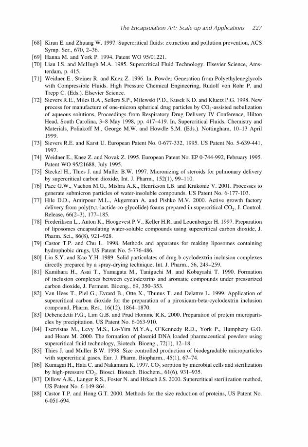
The Encapsulation Art: Scale-up and Applications 227
[68] Kiran E. and Zhuang W. 1997. Supercritical fluids: extraction and pollution prevention, ACSSymp. Ser., 670, 2–36.
[69] Hanna M. and York P. 1994. Patent WO 95/01221.[70] Liau I.S. and McHugh M.A. 1985. Supercritical Fluid Technology. Elsevier Science, Ams-
terdam, p. 415.[71] Weidner E., Steiner R. and Knez Z. 1996. In, Powder Generation from Polyethyleneglycols
with Compressible Fluids. High Pressure Chemical Engineering, Rudolf von Rohr P. andTrepp C. (Eds.). Elsevier Science.
[72] Sievers R.E., Miles B.A., Sellers S.P., Milewski P.D., Kusek K.D. and Kluetz P.G. 1998. Newprocess for manufacture of one-micron spherical drug particles by CO2-assisted nebulizationof aqueous solutions, Proceedings from Respiratory Drug Delivery IV Conference, HiltonHead, South Carolina, 3–8 May 1998, pp. 417–419. In, Supercritical Fluids, Chemistry andMaterials, Poliakoff M., George M.W. and Howdle S.M. (Eds.). Nottingham, 10–13 April1999.
[73] Sievers R.E. and Karst U. European Patent No. 0-677-332, 1995. US Patent No. 5-639-441,1997.
[74] Weidner E., Knez Z. and Novak Z. 1995. European Patent No. EP 0-744-992, February 1995.Patent WO 95/21688, July 1995.
[75] Steckel H., Thies J. and Muller B.W. 1997. Micronizing of steroids for pulmonary deliveryby supercritical carbon dioxide, Int. J. Pharm., 152(1), 99–110.
[76] Pace G.W., Vachon M.G., Mishra A.K., Henrikson I.B. and Krukoniz V. 2001. Processes togenerate submicron particles of water-insoluble compounds. US Patent No. 6-177-103.
[77] Hile D.D., Amirpour M.L., Akgerman A. and Pishko M.V. 2000. Active growth factorydelivery from poly(d,l-lactide-co-glycolide) foams prepared in supercritical CO2, J. Control.Release, 66(2–3), 177–185.
[78] Frederiksen L., Anton K., Hoogevest P.V., Keller H.R. and Leuenberger H. 1997. Preparationof liposomes encapsulating water-soluble compounds using supercritical carbon dioxide, J.Pharm. Sci., 86(8), 921–928.
[79] Castor T.P. and Chu L. 1998. Methods and apparatus for making liposomes containinghydrophobic drugs, US Patent No. 5-776-486.
[80] Lin S.Y. and Kao Y.H. 1989. Solid particulates of drug-b-cyclodextrin inclusion complexesdirectly prepared by a spray-drying technique, Int. J. Pharm., 56, 249–259.
[81] Kamihara H., Asai T., Yamagata M., Taniguchi M. and Kobayashi T. 1990. Formationof inclusion complexes between cyclodextrins and aromatic compounds under pressurizedcarbon dioxide, J. Ferment. Bioeng., 69, 350–353.
[82] Van Hees T., Piel G., Evrard B., Otte X., Thunus T. and Delattre L. 1999. Application ofsupercritical carbon dioxide for the preparation of a piroxicam-beta-cyclodextrin inclusioncompound, Pharm. Res., 16(12), 1864–1870.
[83] Debenedetti P.G., Lim G.B. and Prud’Homme R.K. 2000. Preparation of protein microparti-cles by precipitation. US Patent No. 6-063-910.
[84] Tservistas M., Levy M.S., Lo-Yim M.Y.A., O’Kennedy R.D., York P., Humphery G.O.and Hoare M. 2000. The formation of plasmid DNA loaded pharmaceutical powders usingsupercritical fluid technology, Biotech. Bioeng., 72(1), 12–18.
[85] Thies J. and Muller B.W. 1998. Size controlled production of biodegradable microparticleswith supercritical gases, Eur. J. Pharm. Biopharm., 45(1), 67–74.
[86] Kumagai H., Hata C. and Nakamura K. 1997. CO2 sorption by microbial cells and sterilizationby high-pressure CO2, Biosci. Biotech. Biochem., 61(6), 931–935.
[87] Dillow A.K., Langer R.S., Foster N. and Hrkach J.S. 2000. Supercritical sterilization method,US Patent No. 6-149-864.
[88] Castor T.P. and Hong G.T. 2000. Methods for the size reduction of proteins, US Patent No.6-051-694.

228 Chemical Engineering
[89] Winters M.A. et al. 1996. Precipitation of proteins in supercritical carbon, J. Pharm. Sci., 85,586–594.
[90] Schmitt W.J. 1995. Finely-divided powders by carrier solution injection into a near orsupercritical fluid, AIChE J., 41, 2476–2486.
[91] Forbes R.T. 1998. Supercritical fluid processing of proteins. I: Lysozyme precipitation fromorganic solutions, In, Proceedings of the IChE World Congress on Particle Technology 3,Brighton, UK, pp. 180–184.
[92] Kamihara H., Asai T., Yamagata M., Taniguchi M. and Kobayashi T. 1990. Formationof inclusion complexes between cyclodextrins and aromatic compounds under pressurizedcarbon dioxide, J. Ferment. Bioeng., 69, 350–353.
[93] Steckel H. and Müller B.W. 1998. Metered-dose inhaler formulation of fluticasone-17-propionate micronized with supercritical carbon dioxide using the alternative propellantHFA-227, Int. J. Pharm., 173, 25–33.

9Fine–Structured Materials
by Continuous Coating and Dryingor Curing of Liquid Precursors
L.E. Skip Scriven
9.1 Introduction
Coatings and films produced by depositing a liquid layer and subsequently solidifyingit are vital ingredients of products such as papers for printing; multilayer polymer filmsfor packaging and specialty uses; adhesive labels, patches, and tapes; photographic andgraphic art materials; photoresist preparations and thin sheets of ceramic materials formicroelectronics and other applications; magnetic and optical memory media; electricalconductors, photoreceptor drums, and protective and decorative surface layers in engi-neering, architectural, textile, and manifold consumer materials; and all sorts of laminatesand many other composites. The interior of many coatings and films requires a partic-ular microstructure or nanostructure in order to function as intended, whether optically,photochemically, electronically, magnetically, or mechanically.‘Nanostructure’ commonlymeans scales of 999 nm 0999m downward; ‘microstruc-
ture’ means scales of 01m (100 nm) upward. Coatings deposited as liquids range in solidthickness from around 200 nm to more than 500m. Requisite internal structures rangedown to 12 nm scale, for instance in certain permselective and catalytic coatings.The future will demand continuous processes that deliver fine-scale, intricate, precisely
controlled structures. Indicators for this include the emerging technologies of flat-paneland flexible displays based on variable state encapsulates and on organic light-emittingdiodes, and incipient developments of flexible nanoelectronics based on advanced poly-mers and colloids – all accompanied by visions of lower cost processing on flexible
Chemical Engineering: Trends and Developments. Edited by Miguel A. Galán and Eva Martin del ValleCopyright 2005 John Wiley & Sons, Inc., ISBN 0-470-02498-4 (HB)
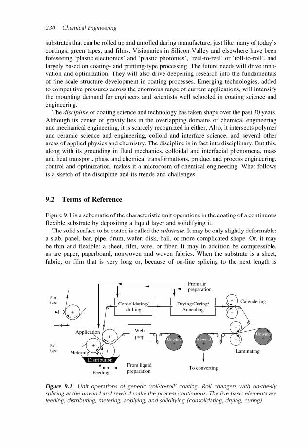
230 Chemical Engineering
substrates that can be rolled up and unrolled during manufacture, just like many of today’scoatings, green tapes, and films. Visionaries in Silicon Valley and elsewhere have beenforeseeing ‘plastic electronics’ and ‘plastic photonics’, ‘reel-to-reel’ or ‘roll-to-roll’, andlargely based on coating- and printing-type processing. The future needs will drive inno-vation and optimization. They will also drive deepening research into the fundamentalsof fine-scale structure development in coating processes. Emerging technologies, addedto competitive pressures across the enormous range of current applications, will intensifythe mounting demand for engineers and scientists well schooled in coating science andengineering.The discipline of coating science and technology has taken shape over the past 30 years.
Although its center of gravity lies in the overlapping domains of chemical engineeringand mechanical engineering, it is scarcely recognized in either. Also, it intersects polymerand ceramic science and engineering, colloid and interface science, and several otherareas of applied physics and chemistry. The discipline is in fact interdisciplinary. But this,along with its grounding in fluid mechanics, colloidal and interfacial phenomena, massand heat transport, phase and chemical transformations, product and process engineering,control and optimization, makes it a microcosm of chemical engineering. What followsis a sketch of the discipline and its trends and challenges.
9.2 Terms of Reference
Figure 9.1 is a schematic of the characteristic unit operations in the coating of a continuousflexible substrate by depositing a liquid layer and solidifying it.The solid surface to be coated is called the substrate. It may be only slightly deformable:
a slab, panel, bar, pipe, drum, wafer, disk, ball, or more complicated shape. Or, it maybe thin and flexible: a sheet, film, wire, or fiber. It may in addition be compressible,as are paper, paperboard, nonwoven and woven fabrics. When the substrate is a sheet,fabric, or film that is very long or, because of on-line splicing to the next length is
Consolidating/chilling
From airpreparation
Drying/Curing/Annealing
Calendering
Laminating
To convertingFrom liquidpreparationFeeding
Rolltype
Slottype
Distribution
Application Webprep
+
+
+
+
+
+
+
+Unwind +
Unwind
+Rewind
+
+
+
+
+
+ +
+
+ +
+Metering
Figure 9.1 Unit operations of generic ‘roll-to-roll’ coating. Roll changers with on-the-flysplicing at the unwind and rewind make the process continuous. The five basic elements arefeeding, distributing, metering, applying, and solidifying (consolidating, drying, curing)

Fine–Structured Materials by Continuous Coating 231
essentially continuous, it is often called a base, a web, or a strip. Web processing meansoperations in which the starting material is unwound from a roll or, with splicing, asequence of rolls, and the finished product is wound up into rolls; this is known inpiece-by-piece technologies as roll-to-roll processing. For steel and aluminum sheet theterm is coil coating or, in some instances, strip coating. The substrate may be rough orsmooth, porous or impermeable. Paper, a rough and porous nonwoven fabric, is probablythe substrate coated in largest amount of tonnage. Substantial amounts of paper andother fabrics are impregnated as they are coated. Steel and aluminum strip, like manyother irregular or rough substrates, is often coated by first coating a rubber-coveredtransfer or offset roll, and then wiping that roll against the substrate to transfer a layer ofliquid. But the most advanced coating technologies produce uniform layers on relativelysmooth polymer films and calendered nonwovens, and on extremely smooth glass andsemiconductor surfaces. In related casting technologies, the liquid layer is deposited onthe very smooth surface of a large roll (rotating cylinder) or endless belt from which itis stripped or peeled after it has adequately solidified.In contrast to all liquid-applied coating is continuous web, wire, or fiber coating.
Spin coating of flat or nearly flat pieces, up to half a meter or so across, is a batchprocess ubiquitous in microelectronics, microphotonics, lab-on-a-chip developments, anda variety of emerging technologies. Another method of coating pieces is to dip them inliquid, then withdraw them slowly and carefully before or as they solidify; this is thebatch version of dip coating – sometimes called withdrawal coating.
The liquid to be coated, or cast and stripped, may be a virtually pure compound,e.g. reactive monomer or molten block-copolymer. Usually it is a solution, a colloidaldispersion, a particulate suspension, a liquid crystal, or a melt. More and more oftentwo or more liquids (almost always miscible liquids) are deposited as superposed layerssimultaneously.In formulating a liquid to be deposited by flow, a crucial factor is its rheology,
specifically its viscosity and viscoelasticity at deposition conditions. Too low a viscositymay leave the deposited liquid layer – especially a thicker one – unacceptably susceptibleto rearrangement by gravity, centrifugal force, air impingement, or drag. Too high aviscosity may unacceptably lower the deposition speed at which not enough air at thesubstrate surface is replaced by liquid. Or too a high viscosity may call for greatermechanical potential gradient (pressure, gravity) than can be made to work in any coatingflow. Such high viscosity liquids fall in the overlapping province of polymer extrusion.Liquids with enough viscoelasticity fall entirely in that province: the criteria are strongenough tensile streamwise and compressive crosswise elastic stress that the relativelysharp turns and highly curved free surfaces of coating flows would cause flow instabilityand nonuniformities.So the liquid to be coated may be Newtonian or virtually so, i.e. with viscosity
independent of shear rate and extension rate (though of course sensitive to temperatureand composition). Its shear viscosity may be anything from the range of water andlow molecular weight organic solvents (0.01 P, or 1 mPa s) to that of concentratedsuspensions and molten polymers of moderate molecular weight (upwards of 1000 P,or 100 Pa s). More often it is shear thinning, with high-shear-rate viscosity toward thelower part of that range. Sometimes, in cases of concentrated particulate suspensions, itis shear thickening and jamming at the highest shear rates seen in coating flows (around106–107/s). Its extensional viscosity may be anything from Newtonian to moderately
232 Chemical Engineering
non-Newtonian (e.g. extension thickening), although relevant extension rates in coatingflows are all too frequently higher than can be attained with contemporary rheologicalcharacterization instrumentation. The liquid may be slightly viscoelastic, even modestlyso, although this, too, is still difficult to characterize. Coating rheology is at the frontierof research and instrumentation.For irregular surfaces and grossly 3D shapes such as the exteriors of vehicles, appli-
ances, and furniture, spray coating is often the method of choice. It is a method in whichliquid solution, with or without particulate pigment, is dispensed through an atomizingnozzle and delivered stochastically as discontinuous droplets, most often with the aid ofan electrostatic field. Once landed on the surface, the droplets must coalesce and, to somedegree, level. Smoothness through leveling is an issue whenever a coating exists as a liq-uid layer before it solidifies. Ink-jet printing is a highly deterministic droplet-depositionprocess that has opened the way to a kind of spray coating that affords exquisite controlof coating thickness and patterns down to submillimeter scale; however, coalescence andleveling remain issues.For thicker coatings on irregular surfaces and 3D shapes the leading alternative to
spray coating is powder coating, which avoids the former’s organic or aqueous solvent. Itis also employed to achieve reproducibly corrugated or ‘wrinkled’ coatings. Oligomer orlow-molecular-weight polymer, cross-linker, and pigments are blended, heated, extruded,cooled, and ground to powder that is dispersed through an electrostatic air gun anddelivered discontinuously as charged particles to the grounded surface. Arriving particlesform a powder layer that is heated along with the substrate and must expel trapped air asit melts, as well as coalescing and leveling to some degree before the molten form curesto high viscosity liquid and then to solid.The liquid phase is not involved in the sputtering, physical and chemical vapor depo-
sition that are common in electronics, magnetics, and photonics. In this important classof processes that create ultrathin coatings – submicrometer down to atomic thicknesses –gas phase constituents are delivered continuously to the substrate surface and once theredeposit, condense, or react. Typically, the structure of the coating is so thin and farfrom equilibrium that it cannot be attained by liquid-phase transport. But when it canbe, low-density gas-phase transport and high heat-release condensation are vulnerable toreplacement by liquid-phase processes such as electrodeposition from a flowing solutionor even drying of a dilute solution layer delivered by a coating flow.Coating by depositing a liquid layer is necessarily followed by some degree of solid-
ification, which means the layer must acquire appreciable elastic modulus and strengthagainst yielding and rupturing. The degree ranges from low in the case of pressure-sensitive adhesives to very high in the case of dense metal oxides. In the related processof casting a film, the stripping or peeling requires a less degree of solidification.In continuous coating, beyond the take-away zone of the coater comes the solidifi-
cation zone, or zones. Solidification may begin by consolidation of a suspension, forexample by liquid sorption into the substrate, or by gelation of a polymer solution orcolloidal dispersion, for example by chilling (as in the case of gelatin solutions) orby heating that induces particle swelling and flocculation (as in the case of plastisols).In hot melt coating and hot embossing, a kind of micromolding, cooling the moltenpolymer is all that is needed. More commonly the deposited liquid layer, or layers, aresolidified by solvent removal, phase change, colloidal coagulation, chemical reaction,or combinations of these. Some coatings such as adhesives barely solidify: all that is

Fine–Structured Materials by Continuous Coating 233
needed is enough polymer entanglement or crosslinking to elevate viscosity and impartsome elasticity. Chemical reactions of addition polymerization and crosslinking or ofcondensation polymerization, often referred to as curing, may be induced or hastenedby activating catalysts. Activation can be by exposure to moisture or oxygen, by out-diffusion or breakdown of blocking agents, by heating, or by radiative bombardmentwith ultraviolet light or electron beam. However, the commonest means of solidificationis solvent removal by hot-air drying, though this may be accompanied or followed bycuring to arrive at the needed hardness, toughness, insolubility, or impenetrability.If the coated liquid contains highly volatile components, the drying zone may intrude
upstream into the take-away zone and even into the coating bead; this is often a leadingcomplication of solvent coating as against water-borne coating. Likewise if the liquid ispolymerizable and reaction is already initiated, the curing zone may intrude upstream;or if the liquid is actually a suspension and on the verge of colloidal instability, theflocculation zone may intrude upstream. Generally it is advantageous to separate coatingand solidification in order to be able to control better each of these two parts of anycoating process.Coating and solidification are of course closely linked: typically, the more fluid the
starting liquid, the easier it is to feed, distribute, meter, and deposit on the substrate; butthe more drying or reaction it takes to solidify. For example, the greater the amount ofdissolved polymer in a solution coating, the less solvent there is to remove by drying, butthe higher the viscosity and viscoelasticity of the liquid and the harder it is to coat well.Similarly, the higher the volume fraction of particles in a suspension coating, the lesssolvent there is to dry, but the higher the viscosity and difficulties of coating. Similarlyagain, the higher the degree of oligomerization of a ‘100 percent solid’ reactive coating,the less the polymerization, crosslinking, and stress development in the curing step, butthe more viscous and difficult to coat is the precursor oligomer or polymer. On the otherhand, the lower the viscosity (and the greater the thickness) of a liquid layer arriving ata drier, the weaker the convective airflow that can unlevel it, and so the more gently itsdrying must begin. Thus there is a basic trade-off between the coating and solidificationparts of a process.
9.3 Depositing a Liquid Layer
9.3.1 Coating Flows
An astonishing variety of methods have been developed for delivering a liquid phasecontinuously in industrial practice. The highly simplified diagrams of Figure 9.2 includemost of the methods of any importance. Those called two-layer slot, multilayer slide, andmultilayer curtain are the ones by which two or more superposed layers can be depositedsimultaneously. Not only do they avoid inefficiencies of coating and drying each layerof a multiple-layer structure in succession, they also make carrier layers and uncoatablythin layers possible.Dip coating, the first two diagrams, is perhaps the simplest and probably the oldest
way of depositing a precisely uniform layer of liquid less than a poise or so in viscosity.The faster the surface is withdrawn from the coating bath or the higher the liquid’sviscosity, the thicker the layer that is formed, up to a limit. Consequently, dip coating

234 Chemical Engineering
Figure 9.2 Coating flows: simplified diagrams
is today seldom encountered outside the laboratory, except in the second diagram wherethe surface being coated is a ‘pick-up’ roll partly immersed in a pool of liquid of modestviscosity so that as it turns it carries away a layer that can be thinned or split before it iscoated or stripped.

Fine–Structured Materials by Continuous Coating 235
Monolayer transfer coating, the last diagram, represents the ultimate in thin layerdeposition, because anything less than a coherent molecular monolayer simply does notconstitute a coating. First demonstrated by Katherine Blodgett over 60 years ago in IrvingLangmuir’s laboratory, monolayer transfer coating has continued to be a ticklish, slow,batch process. With the upsurge during the past decades in creating ultrathin coatingscontaining molecular-scale structures, studies were launched in many places that havenot yet led to an industrially applicable continuous process, but may ultimately do so.To understand the variety of methods and how they relate to one another, it is helpful
to recognize that they all perform the same set of basic functions.
9.3.2 Basic Functions in Coating
All of these coating methods perform four of the five basic functions one way or another.They feed liquid through a pipe, or sometimes a manifold of pipes, and distribute it acrossthe width of the coater, which is no less than the width of the substrate to be coated.They meter the flow rate or they meter the coated layer to the required wet thickness.They apply the liquid coating to, or deposit it on, the substrate, or web, displacing mostof the air (or other gas) that originally contacts the surface. Indeed, to coat is to replacegas at a substrate surface by a layer of liquid. Beyond these four functions – feeding,distributing, metering, and applying – there is a fifth. That is to solidify the coating; itmay be necessary also to anneal it to reduce residual stresses or develop structure. Thebasics of solidification are examined below.
Feeding. Whenever liquid is applied to a substrate in excess and the excess is subse-quently metered off, the feed method is not critical. This situation is sometimes calledpost-metering, in contrast to pre-metering. Nor is the feed method critical when distribu-tion is by a pond or pool with overflow. Whenever liquid is not applied in excess – inother words, when all the liquid fed is coated – the feed method does become critical.This is the situation called pre-metering. Volumetrically controlled feeding is most oftenaccomplished by a positive displacement pump operated as a meter, i.e. under smallenough pressure difference that the leakage flow through the pump is tolerable. The term,feeding, is also applied to arrangements that combine feeding, distribution, and in someinstances metering functions as well, to supply a layer or film of coating to the entirewidth of the next element in a coating operation. Prime examples are slot feeding andslide feeding of curtain coating and various arrangements used in roll coating. Multilayercoating, which is the simultaneous application of two or more layers of coating liquid,generally requires that each layer be separately pre-metered.
Distribution. From the supply pipe or delivery point, the coating liquid must be spreadto the width to be coated, or perhaps to somewhat greater width. Simplest is a poolin a pan from which liquid is withdrawn by a roll or by substrate dipping into it orby substrate passing through it. The pool’s simplicity comes with potential for greatdifficulties, however. Open pools are prey to sloshing, bubbles and foam generated byarriving liquid, roll surface, or substrate; to waves excited by ever-present mechanicaland acoustical vibrations; to contamination falling out of the air overhead; to evaporationof volatile components into the air overhead, and resulting concentration gradients inthe remaining liquid; and to long mean residence time. The outcome of the last canbe disastrous for coating liquid that is reacting chemically or colloidally to form, for

236 Chemical Engineering
example, extra-viscous gobs, blobs, or flocs. Consequently, there is a universal hierarchyof improvements to simple pool distribution: splashing and sloshing are reduced, the panis covered over, the free liquid surface is made smaller, the pan is shaped and shrunkin size, and ultimately evolves into a distribution chamber. Pressure difference mustbe employed, and in such a way that the pressure across the width of the distributionchamber is close enough to being uniform.Feed liquid is spread across die coaters, slot and extrusion coaters, slide and many
curtain coaters by chamber-and-slot distribution. The liquid is introduced into a chamberor manifold as long as the coating is to be wide, which delivers the liquid in turn toa narrow slot through which it flows to an exit aperture where it may be applied to asubstrate, turn and run down an apron or slide, or fall free as a curtain.When the flow per unit width across the exit aperture of a chamber-and-slot arrange-
ment can be made uniform enough, distribution doubles as metering. Indeed, the distribu-tion and metering functions are inextricably combined in this manner in slot, extrusion,slide, and curtain coaters that employ chamber and slot and operate in the pre-meteredfeed mode. The combination is ubiquitous in multilayer coating.
Metering. The ultimate would be to generate a liquid layer of perfectly uniform thicknessand microstructure on a perfectly smooth substrate. This can be approached by applying adistributed excess of coating liquid and metering off the excess, that is, by post-meteringas in bar, rod, and blade coating. Or, it can be approached by distributing and pre-metering the liquid directly onto the substrate, as in extrusion coating and sometimescurtain and slide coating. Or, it can be approached via pre-metering onto a perfectlysmooth intermediate substrate and then applying, or transferring, the layer to the finalsubstrate, as in some kinds of roll coating.Ideal pre-metering delivers a layer or layers of uniform thickness everywhere regardless
of the topography of the substrate (any subsequent leveling flow might reflect thattopography as it shifted liquid so that the pre-metering action was partly undone). Idealpost-metering delivers a single layer of thickness so modulated to the substrate topographythat the surface of the liquid is uniformly smooth. Ideal smoothing, or planarization as itis known in microelectronics technology, is a type of re-metering that converts a liquidlayer whose surface is not smooth into one whose surface is, without altering the averagecoat weight, i.e. the average layer thickness.There is an intermediate category of in situ metering that pertains to situations where
metering and application take place simultaneously, as in those kinds of roll coating thathave substrate (web) in the metering gap. Then the substrate, its thickness variations, andfailures to lie tight against the roll that carries it all contribute to the local thickness ofthe liquid layer that is deposited.The advantage of gravure-roll metering can be accurate metering of a liquid layer
that is on average quite thin, but at the expense of re-metering the layer by smoothing.A further cost can be that of controlling the metering action at the cell level, which maybring extensional viscous force into prominence and viscoelastic forces too if the liquidcan develop them. These can give rise to deleterious filamentation and misting as coatingspeed rises. Electrostatic force is not infrequently deployed to assist in achieving thedesired action.Compliant-gap metering is characterized by one or both gap walls, or their mountings,
being deformable by forces developed in the flowing liquid. Those forces are pressureabove all, but also viscous wall shear and, in certain nonlinear and many viscoelastic
Fine–Structured Materials by Continuous Coating 237
liquids, extra normal forces. As a wall or its mounting deforms, its elasticity adds toany opposing force preloaded onto it, until that force sum and the hydrodynamic forcesexerted by the liquid come into balance in a state that is steady – apart from unavoidablefluctuations in time, for example when rough or porous substrate is being coated. Asa wall deforms, the gap through which the liquid flows changes, and so do the forcesexerted by the liquid. Thus the compliance, or elastic response, of the walls and the flowof the liquid are coupled together. Such situations are the subject of elastohydrodynamics;hence compliant-gap metering can also be called elastohydrodynamic metering.
Application. This is the basic action of turning a more or less dry substrate or web intoa wet one, and it can be carried out before or after the metering function, and even aspart of the distribution function. The heart of application is the dynamic wetting zone,which looks like a ‘line’ and is often called one, although it is in fact a microscopic orsubmicroscopic region in which wetting forces are active and the coating liquid replacesgas at the solid surface.Two free surfaces are present in every coating flow. One extends from a separating
contact line (the ‘upstream’ one), a static contact line where it departs from a wall ofthe coating set-up, to the wetting ‘line’ where it meets the substrate surface. This freesurface is the key player in the basic action, to coat: it becomes the interface between theliquid layer and the substrate to which it is applied. The closer the upstream separatingcontact line is to the dynamic wetting line, the more desirable for precision coating it isto design the coating set-up and operation so that the separating contact line is straight.The other free surface originates at another separating contact line – the ‘downstream’
one – a static contact line where it departs from a wall of the coating device, and extendsdownstream to become the free surface of the coated liquid (where it may be subjectedto smoothing or allowed to level). The shorter the distance between the downstreamseparating contact line and the free surface of the coated layer, the more critical forprecision coating it is that the separating contact line be perfectly straight, a conditionbest attained by giving it a straight sharp edge to attach to and then operating so thatit does. The region between the two free surfaces is, in many cases, called the ‘coatingbead’. There, especially, flow nonuniformity and unwanted microvortices can influencethe final microstructure of multilayer coatings and coatings containing acicular, tabular,or other types of particles.Plunging application takes place where substrate enters an open pool, pond, puddle,
or fountain. Flow around the dynamic wetting line is comparatively unconfined so thatthe free surface, which is the upstream one, is fairly free to deform into a local meniscusand ultimately to entrain air. Generally, the substrate exits elsewhere and so there is nocompact coating bead.Confined flow application takes place where substrate enters the liquid through an
upstream meniscus confined in a slot, or a slit sealed by a flexible blade, or a gapbetween walls, one or both of which are moving. Flow around the dynamic wetting lineis comparatively confined, and the upstream free surface is less free to deform and canbe manipulated by applying vacuum or electrostatic field, which may delay unacceptableair entrainment to higher substrate speeds. In slot and slide configurations, vacuum orelectrostatic field can be used to draw the bead further upstream in the gap, therebyenlarging the micro-reservoir for re-metering, which may be desirable. The bead may,however, develop microvortices, which are not desirable though they seem often to betolerated.

238 Chemical Engineering
Impingement flow application is what is seen in curtain coating and extrusion coating,where a pre-metered layer of liquid arrives as a free film that attaches at the dynamicwetting line. If the curtain is not short, the falling liquid may have enough momentum toaugment the pressure there and delay excessive air entrainment to higher substrate speed.Electrostatic force may be deployed around the dynamic wetting line to achieve the sameend in both curtain coating (‘electrostatic assist’) and extrusion coating (‘electrostaticpinning’). Raising the curtain height can cause the impinging flow to bulge upstream in a‘heel’; a slight bulge provides a little pre-metering, which may be desirable, but a largerone reduces impact pressure around the dynamic wetting line and ultimately developsmicrovortices and unwanted recirculation within the heel.Transfer application employs a compliant gap to apply most of an arriving pre-metered
layer to substrate passing through the gap. The compliant element can be either a softtransfer roll (often called an applicator roll), a soft backing roll, or the web tensionedover a transfer roll.More complicated mechanisms are active in application of coating from knurled and
gravure rolls used for metering and transfer. The basic action at the dynamic wetting linein both forward and reverse modes may be influenced by the pattern of grooves or cells,even favoring entrainment of microbubbles as has been reported from studies of gravureprinting. The film splitting or wiping is accompanied by partial emptying, or ‘pick-out’of the grooves or cells; control of the fraction transferred is critical to the metering thatis combined with the application.Because each of the four basic functions can be accomplished in multiple ways, the
number of combinations into coating methods is large.
9.3.3 Physics of Coating Flows
In a coating flow the gas originally in contact with the solid surface is replaced in anaction known as dynamic wetting (Figure 9.3). This action appears to the eye, evenwith the help of optical magnification, to take place at a line, or curve, a seemingly 1D‘thing’. This thing is called the wetting line or the (apparent) dynamic contact line. Itis present in every coating flow and it is the biggest scientific unknown although notalways the most important practical aspect. In start-up of slot and slide coating, dynamicwetting is established by liquid breaking through gas entrained by the moving substratesurface; that it does so is crucially important. The physics of dynamic wetting is still notwell resolved in terms of basic principles. Whatever happens on the invisible scales ofmolecules and surface roughness, the arriving liquid appears to slip locally. In all othercircumstances, liquid in contact with a solid surface does not appear to move relative tothe surface. Thus the no-slip boundary condition that is so firmly established elsewherein fluid mechanics (though not so firmly in polymer processing) must fail near a dynamiccontact line – which is of course a 3D region, albeit a submicroscopically slender one.The visible contact angle at a wetting line or dynamic contact line is called the (apparent)dynamic contact angle. Generally, it differs from the (apparent) static contact angle thatthe same liquid and gas seem to make with the same surface when all are at rest.At the edges of the coated layer its free surface ends in ordinary static contact lines.
These lateral contact lines necessarily bend round upstream and connect with the wettingline. Thus at each edge of the layer where it is being delivered to the substrate theremust be a curved segment of dynamic contact line, and the apparent slip of the liquid

Fine–Structured Materials by Continuous Coating 239
Apparent dynamiccontact line
Apparent dynamiccontact angle
Displacedgas
Becomesstatic
at edge
Dynamiccontac
line
OBLIQUE VIEW
Coated liquid layer
Gas
Gas
Substrate
Solidification
Dynamic contact lineis a gas–liquid flow!
Entrained gas
Coating liquid
Substrate
Figure 9.3 To coat is to replace gas with liquid at a solid substrate
must cease by the place that segment turns into a completely static, lateral contact line(Figure 9.3). A static contact line or separating line may locate other than where it issupposed to, thereby marring or destroying the uniformity of coating. Control of contactline attachment is crucial to precision coating. Solid corners of small and uniform radius(as little as 25 m) are useful; wettability discontinuities are less so. Sloppy start-up canoverwhelm a careful design.A dynamic contact line, or wetting line, may pass visible amounts of the gas originally
at the solid surface, thereby destroying the uniformity of the coating; short of this it maypass invisible amounts of gas that wreak havoc during subsequent heating and drying,or that impair product function. The issue is air entrainment (Figure 9.3). The onset ofunacceptable air entrainment sets an ultimate limit on coating speed. At a speed less thanthat, the dynamic contact line may begin bending and looping, or oscillating in position,interposing another limit.
9.3.4 Experimental Analysis
Each coating method has limits within which the flow can even exist, and narrower oneswithin which it is close enough to 2D and steady to deliver the desired uniformity. Thequality window is generally smaller, the greater the uniformity sought. Quality windows,like the operability window, are in the ranges of design parameters like lip shapes and

240 Chemical Engineering
roll runout, operating parameters like web speed and coating gap, and formulation prop-erties like low-shear viscosity and equilibrium surface tension. Typically, the industrialapproach is a ‘designed experiment’ to find out if a given formulation ‘can be coated’,i.e. whether a continuous liquid layer forms and persists, and if ‘defects are excessive’,i.e. whether the layer is adequately uniform. A more fruitful approach is using eyes,lights, and stroboscope, and then more advanced flow visualization techniques to seewhat actually happens – how the layer fails to form, how flow instabilities and otherdefects arise – and thereby to seek the responsible mechanisms.Coating flows though laminar are made complex by the freedom of the liquid’s surfaces
and by the abrupt changes in direction and speed of the liquid where it passes from theapplicator device to the solid substrate. Rigid substrates may move past at tenths of metersper second, flexible webs and fibers up to tens of meters per second. Often the flows areeven more complicated by viscosity changes with the rates at which the liquid is locallysheared and extended, and by traces of viscoelastic behavior. The scale is small in twodirections, along the flow and through the flow. That makes magnification necessary andillumination difficult. If the liquid or a surrogate for it is clear and transparent, markerparticles or dye traces are necessary: hydrogen bubbles, aluminum flakes, and fluorescentdyes are all suitable in various circumstances. The scale is large in the third direction,across the flow, and the edges differ to some degree from the rest of the width. Thatmakes long working length lenses and special edge plates obligatory for side views, andputs a premium on 2D sectioning by optical means.Figure 9.4 shows Sartor and Suszynski’s pioneering arrangement for slot coating where
the slot is 250 m or more across and the gap between die lips and substrate is inthe same range; it drew on Schweizer’s then unpublished breakthrough visualization ofslide coating. Cohen and Suszynski’s splendid view appears in Figure 9.5; the hydrogenbubbles and dye streaks make plain the menisci that bound the coating bead, the intensemicrovortex within it, and the streamlines leading to the coated layer carried away onthe upward-moving substrate.Crookedness of contact lines and crossflow nonuniformity is best assessed from plan
views through transparent substrate. In tensioned-web coating methods, clear web affords
Figure 9.4 Set-up for visualizing slot coating flow, in a cross-section to show streamlinesand free surfaces

Fine–Structured Materials by Continuous Coating 241
Figure 9.5 Cross-sectional view of slot coating flow
Figure 9.6 Transparent glass roll finished and mounted with ±05m run-out. Visual accessto plan views of flow in a coating bead is through the hollow shaft or under the can-tilevered end
the needed optical access. For other methods, the web carried on a back-up roll can bereplaced by a transparent roll, as shown in Figure 9.6. The third panel of Figure 9.7was obtained in this way (equivalent views of wire-wound rod and gravure coatingwith rubber-covered back-up roll were obtained by devising transparent rubber covers).Figure 9.7 summarizes the challenges of visualizing internal features of coating flows.Further information and examples are recorded by Suszynski and Scriven in ChemicalEngineering Progress, September 1990, pp. 24–29, and by others in published theses(see Literature section) and papers.Interpreting the results of flow visualization and measurement takes theory, and theory
requires flow properties: viscosities as functions of shear and extension rates, peculiarviscoelastic parameters if the coating liquid is mildly viscoelastic solution, surface tension

242 Chemical Engineering
Transparent backing roll
Mirrors
Fiberscope
Direct unobstructed line of view
Special design features ofapplicator
Transparent substrate and/orliquid layer
Visualization of internal flow features
Figure 9.7 Equipment must often be specially designed to provide optical access to thecoating bead
and its dependence on concentration if that is a factor (in which case a suite of diffusion,adsorption, and micellization properties may also be vital), appropriate contact anglesat static contact lines and apparent contact angles at dynamic ones. Diffusivities andsolution activities may be needed to understand growth of interlayer diffusion zones inmultilayer coating. Getting the needed flow properties is often so difficult that riskyguesses must suffice. Deformation rates in shear and extension in many coating flowsare much higher than those attainable in laboratory rheometers. Static contact angle datatend to be crude and plagued by slow equilibration, or ‘hysteresis’. Apparent dynamiccontact angle is not a property, but a microscopic two-phase process, 3D and unsteadyin detail; purported correlations of it can be useless for getting at limits of coating speed.Needs and opportunities in this arena are great.
9.3.5 Theoretical Analysis and Engineering
Coating flows of liquid lend themselves to practical and scientific understanding forthree reasons: they are laminar, steady, and 2D to a good first approximation. They arenecessarily laminar to create and maintain uniformly thick layers with desired internalstructure, including stacking of multiple layers deposited simultaneously. They are nec-essarily steady to create uniformly thick layers in the direction of the substrate’s relativemotion (‘downweb’); exceptions, however, are periods of start-up, shutdown, and splicepassage – and the entirety of the wonderful process of spin coating. They are necessar-ily 2D, which here includes axisymmetric, to create layers that are uniformly thick inthe direction transverse to the substrate’s relative motion; exceptions are the edges ofplanar coatings and starts and stops in general. A second approximation is required toaccount for departures from steadiness and two-dimensionality caused by: out-of-flatness(or out-of-roundness), roughness, and porosity of substrate; imperfections and, in certain

Fine–Structured Materials by Continuous Coating 243
cases, special features of coater design and operation; and sometimes perhaps tolerablesecondary flows inherent to particular circumstances. These are all challenges to analysis.The key to understanding flow coating is the physics of the forces involved. These
forces are: viscous, pressure, and capillary pressure (surface tension resultant in curvedinterfaces); sometimes gravity, inertia (curvilinear acceleration), surface tension gradient,and elastic responses of compliant confinement (as in ‘elastohydrodynamics’); occasion-ally viscoelastic effects, electrostatic, and magnetic forces; always, at contact lines andsmall scales elsewhere, the London-van der Waals and other forces of electromagnetic ori-gin known as ‘surface forces’, which give rise to disjoining pressure; and constantly in thebackground the very small buffeting forces of thermal fluctuations in the liquid (‘Brow-nian forces’). Today the forces are being analyzed, predicted, and managed by design atfour levels: (1) Engineering approximations are sometimes adequate – the lubricating flowand related viscocapillary flow approximations are more and more being developed andused in ranges where they have been validated by more exact Navier–Stokes or relatedtheory. (2) Commercial computational fluid dynamics software for solving the equationsof Newtonian (Navier–Stokes) flow and generalized Newtonian flow (shear-rate sensitiveviscosity) is still limited but advancing and it can already be extremely useful, as in diedesign and certain templated 2D coating flows. (3) Advanced, tailored codes are beingdeveloped by specialists in large corporations, small entrepreneurial firms, and govern-ment laboratories, often drawing on the next level. (4) Pioneering research programsin viscous free-surface flows are being conducted in a few universities worldwide. Thebest validation of a solution is with whatever experimental measurements are available,whether merely the shape of a free surface, or the occurrence of a microvortex, or thestreamlines and local velocities of the flow. Figure 9.8 is a steady-state example fromK.S.A. Chen’s research on simultaneous precision coating of multiple miscible layersassembled from successive feed slots in the inclined surface of a slide die.For purposes of design, control, and optimization a steady-state solution – an operating
state – is not enough. Many solutions are needed, even in the most parsimonious probing
Figure 9.8 Two-layer slide coating flows: visualization flow field versus computed flow field.Two microvortices are obvious; another may be present on the slide

244 Chemical Engineering
of parameter space. Many solutions are needed in order to get an idea of the ranges ofdesign parameters and operating parameters within which steady, 2D flow states exist.Arc-length continuation also makes it possible to discover when more than one such flowstate exists, a not uncommon situation, and the relative stability of the multiple states.Augmented continuation schemes make it possible to track turning points themselvesthrough parameter space, a procedure called fold-tracking. This procedure can be usedfor delineating windows of feasible operation.Within a feasibility window lie coating quality windows defined by features and
sensitivities of the flow states. Similar augmented continuation schemes make it possibleto track through parameter space the limiting states at which a microvortex appears ordisappears, a static contact line pins to an edge or moves free, a machining flaw createsan unacceptably thick streak, and so forth – and in addition to see how the feasibilityand quality windows depend on shape and dimensions of the coating applicator.Quality windows are also delineated by set values of the damping coefficients and
attenuation factors that are computed in stability and frequency analysis. These too canbe traced out efficiently in parameter space by augmented continuation schemes. Thesame is true of the turning points and bifurcation points in parameter space, points ofmarginal stability. These are the guides to situations in which there is more than onestable operating state. When such situations may arise, it becomes desirable to solverepeatedly the full equation system of flow for transient behavior in order to know howdifferent start-up procedures and upsets select among the multiple stable states.Fold-tracking, feature-tracking, stability and frequency analysis, and transient analysis,
all now demonstrated in conjunction with the computational fluid mechanics of coatingflows, are potent tools for process design, control, and optimization. Edge effects andother 3D free-surface phenomena are challenges that have had scant theoretical analysis.Current theory-centered research is on aspects of coater shape optimization and activeflow control. Rational engineering of coating flows, whether to advance establishedtechnology or to produce new lines of fine-structured coatings, is a field wide open tochemical engineers in industry and academia.
9.4 Solidifying the Liquid Layer
The basic function of solidification can be accomplished in a variety of ways, someof them already noted (Figure 9.9). The principal ones are: solvent removal from thesurfaces of a coating; solvent movement to the surfaces from within a coating; colloidaltransformations, phase separations, fusion, and binding; polymerization (both growthby chain-extension or condensation-addition reactions, and networking by crosslinkingreactions) and other chemical reactions of curing; initiating and speeding the reactionsby controllable catalysts and, in some cases, radiations; and energy delivery to supplythe latent heat of evaporating solvent or to initiate or drive the chemical reactions. Atone extreme, solidification is a simple matter of solvent diffusion to and removal fromthe surface of the coating; at another extreme, the coated liquid is entirely monomer oroligomer that can be polymerized in place, so that no solvent whatsoever is involved.Residual monomer or oligomer can be as difficult to remove during processing and asobjectionable in storage and use as residual solvent, however.

Fine–Structured Materials by Continuous Coating 245
Festoon drier,gentle air flow
+ + + +
++
+
+
+
++
+
+
+ +
+ +
+ + + +
+ + + +
+ +
+
+ + +
Heated rolls,mild air flow
Tunnel drier,roller transport,counter air flow Catenary drier,
fitted aircaps
Helicalflotation
drier
Condenser drierwith floated webFloatation drier
Impingment drier,roller transport
Heated drumdrier with
air cap
Spiral drier,roller transport,mild crossflow
COLD PLATE
HOT PLATE
Figure 9.9 Drying and thermal curing: simplified diagrams
Solvent removal. Evaporation of solvent from the exposed surface of a coating intothe adjacent air or other gas is the usual means of solvent removal. Because diffusioninto stagnant gas is a relatively slow process, it is generally augmented by convectivesweeping of the coating surface. Sometimes the sweeping is by weak and irregularnatural convection and room air currents, as in the slow dip coating often used in thelaboratory to coat thin films – as thin as one surfactant molecule or polymer moleculethick. A layer dipped at millimeters per minute is so thin that natural convection may beadequate to remove the tiny amount of solvent present even when the solvent is initiallyat high concentration. Sometimes the sweeping is by strong and reproducible inducedconvection, as in the ubiquitous spin coating commonly used in both the laboratory andthe factory to coat thin films onto plates, disks, and wafers. The spinning substrate isitself a pump that draws gas around the axis of rotation toward its coated surface and thendrives the gas radially outward over the coating. In dip and spin coating, the meteringof the coating by flow and the solidification by evaporation can be, and frequently are,combined into a single operation. Doing this successfully can require elaborate control ofthe flowing gas and its solvent content in order to sequence or balance the two functionsoptimally.In festoon driers and some tunnel drying operations (cf. Figure 9.9), gentle convective
sweeping of the coated web by low-velocity crosswise air flow is sufficient to removeevaporated solvent. The same can be true of terminal zones of drying and curing ovensused to lower residual solvent by out-diffusion and residual stress by annealing. Wheresolvent is to be removed rapidly, strong sweeping by forced convection of air or othergas is used. The notable exception is rapid solvent removal by simple diffusion acrossgas flowing laminarly in a carefully controlled gap. The gap can be made so narrow thatthe rate of diffusion is quite high, as in condensation drying.The mass transfer coefficient is highest when the gas flow is perpendicular to the
evaporating surface because then the diffusion of vaporized solvent off the surface ismost enhanced by convective action. When the drying rate is extreme, the vaporizing
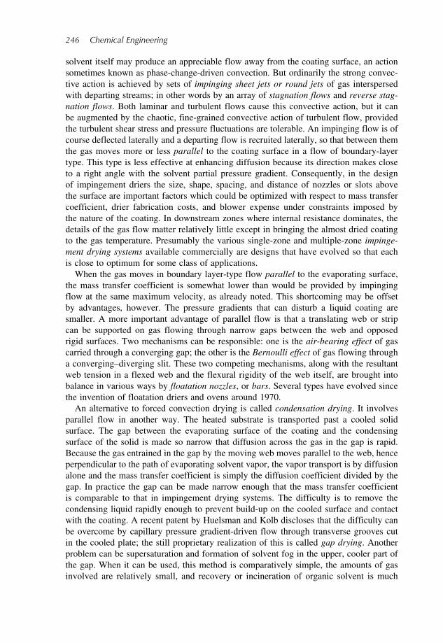
246 Chemical Engineering
solvent itself may produce an appreciable flow away from the coating surface, an actionsometimes known as phase-change-driven convection. But ordinarily the strong convec-tive action is achieved by sets of impinging sheet jets or round jets of gas interspersedwith departing streams; in other words by an array of stagnation flows and reverse stag-nation flows. Both laminar and turbulent flows cause this convective action, but it canbe augmented by the chaotic, fine-grained convective action of turbulent flow, providedthe turbulent shear stress and pressure fluctuations are tolerable. An impinging flow is ofcourse deflected laterally and a departing flow is recruited laterally, so that between themthe gas moves more or less parallel to the coating surface in a flow of boundary-layertype. This type is less effective at enhancing diffusion because its direction makes closeto a right angle with the solvent partial pressure gradient. Consequently, in the designof impingement driers the size, shape, spacing, and distance of nozzles or slots abovethe surface are important factors which could be optimized with respect to mass transfercoefficient, drier fabrication costs, and blower expense under constraints imposed bythe nature of the coating. In downstream zones where internal resistance dominates, thedetails of the gas flow matter relatively little except in bringing the almost dried coatingto the gas temperature. Presumably the various single-zone and multiple-zone impinge-ment drying systems available commercially are designs that have evolved so that eachis close to optimum for some class of applications.When the gas moves in boundary layer-type flow parallel to the evaporating surface,
the mass transfer coefficient is somewhat lower than would be provided by impingingflow at the same maximum velocity, as already noted. This shortcoming may be offsetby advantages, however. The pressure gradients that can disturb a liquid coating aresmaller. A more important advantage of parallel flow is that a translating web or stripcan be supported on gas flowing through narrow gaps between the web and opposedrigid surfaces. Two mechanisms can be responsible: one is the air-bearing effect of gascarried through a converging gap; the other is the Bernoulli effect of gas flowing througha converging–diverging slit. These two competing mechanisms, along with the resultantweb tension in a flexed web and the flexural rigidity of the web itself, are brought intobalance in various ways by floatation nozzles, or bars. Several types have evolved sincethe invention of floatation driers and ovens around 1970.An alternative to forced convection drying is called condensation drying. It involves
parallel flow in another way. The heated substrate is transported past a cooled solidsurface. The gap between the evaporating surface of the coating and the condensingsurface of the solid is made so narrow that diffusion across the gas in the gap is rapid.Because the gas entrained in the gap by the moving web moves parallel to the web, henceperpendicular to the path of evaporating solvent vapor, the vapor transport is by diffusionalone and the mass transfer coefficient is simply the diffusion coefficient divided by thegap. In practice the gap can be made narrow enough that the mass transfer coefficientis comparable to that in impingement drying systems. The difficulty is to remove thecondensing liquid rapidly enough to prevent build-up on the cooled surface and contactwith the coating. A recent patent by Huelsman and Kolb discloses that the difficulty canbe overcome by capillary pressure gradient-driven flow through transverse grooves cutin the cooled plate; the still proprietary realization of this is called gap drying. Anotherproblem can be supersaturation and formation of solvent fog in the upper, cooler part ofthe gap. When it can be used, this method is comparatively simple, the amounts of gasinvolved are relatively small, and recovery or incineration of organic solvent is much

Fine–Structured Materials by Continuous Coating 247
easier. The drier zones are smaller than when forced convection is used. Moreover, thegas exerts virtually uniform shear stress and pressure on the coating’s surface and sodoes not disturb the uniformity of its thickness.
Solvent movement within coatings. The mechanisms by which volatile solvents canmove within a coating as it solidifies are few: pressure gradient-driven flow in a porouscoating, and diffusion along with diffusion-induced convection (or ‘diffusion-engenderedflow’) in general. Though the mechanisms are few, the complexities are many.If a coating is, or becomes, porous, liquid can flow within it in response to differences
in capillary pressure at the menisci between liquid and gas. If the liquid wets the porewalls, the flow is away from less curved menisci, which reside in larger pores, andtoward more curved ones, which reside in smaller pores; if the menisci are all of aboutthe same curvature but are at different temperatures, the flow is from the hotter onestoward the cooler ones. If liquid should happen to exceed its bubble-point and boilanywhere within the porespace, the pressure there tends to drive liquid away and out ofthe porespace, as in so-called impulse drying of paper. If the solid of the matrix shrinks,stress is transmitted as pressure to liquid in the porespace and the liquid flows in responseto any gradient of pressure that arises. If the coating and substrate together make aporous sheet, liquid can be driven toward one side by applying high enough gas pressureon the other side. In every case the local flux of the flowing liquid is proportional tothe local pressure gradient. The proportionality factor is the property called porespacepermeability, divided by the viscosity of the liquid. The viscosity can be quite sensitiveto liquid composition and temperature. Measurements of these properties for solidifyingcoatings are scarce, and estimating them may be difficult. Nevertheless, they are keys tounderstanding convective flow in porous coatings, as theoretical modeling of the flowprocesses makes clear.Solvent in solution with other soluble components diffuses in response to differences
in composition (chemical potential, actually). Within a given phase, it tends to diffusefrom regions of higher concentration toward regions of lower concentration – always inbinary solutions, but not always in multicomponent systems. In a binary solution onlyone mole fraction or mass fraction is independent, and so the local diffusional flux ofeither component is proportional to the local gradient of mole fraction, mass fraction, orconcentration. The proportionality factor is the binary diffusion coefficient, or diffusivity.Generally it depends on concentration, and the dependence can be extreme when theconcentration of solvent in a polymer is low – as in the late stages of drying a solvent-borne polymeric coating. Furthermore, the diffusion coefficient can lag in its response tofalling concentration, giving rise to a version of what is called ‘non-Fickian diffusion’.This is probably one of the causes of the phenomenon of skinning in which a solvent-stripped layer at the surface of a rapidly drying coating develops enough resistance todiffusion to seal off effectively solvent remaining deeper in the coating. The body ofmeasurements of binary diffusivities relevant to coating formulations is growing andestimation procedures are advancing. The complication in multicomponent systems is thatgradients of other components can contribute to the diffusion flux of a given component.This can produce puzzling distributions of solutes in drying coatings. Measurementsof ternary diffusion coefficients are rare, and estimating them even roughly is difficult.Nevertheless, the diffusion coefficients are keys to understanding solvent transport insolidifying coatings, as theoretical modeling of drying and curing makes clear. The needfor data is great.

248 Chemical Engineering
Heat delivery. Convection and conduction from hot gas sweeping by is the leadingmode of heat transfer to a drying coating to supply the latent heat of vaporization ofsolvent. Except when solvent evaporation is so very rapid as to produce an appreciableconvective velocity away from the surface, in turbulent gas flow the mechanisms ofheat transfer to and solvent transfer away from the evaporating surface are virtuallyidentical combinations of convective action with thermal conduction on the one hand andmolecular diffusion on the other. This is reflected in useful correlations, like Colburn’s,of the mass transfer coefficient with the more easily measured heat transfer coefficientin turbulent flow. It is also the reason that the now fairly extensive literature on theperformance and design of driers focuses on heat transfer coefficients and heat deliveryrates.However, the correlation of mass transfer with heat transfer is relevant only to the heat
transferred directly to the evaporating surface. That other modes of energy delivery canbe highly useful and have to be considered separately is well appreciated in the literature.
Phase separations and colloidal transformations. A liquid is coated in order to delivermaterial that will end up in a solid or semi-solid form on the substrate. Temporarysolidification may be achieved by consolidating suspended particles, for example byliquid sorption into the substrate, or by gelling polymer solution, for example by chilling.To dry a coating is to remove enough volatile solvent that the remaining material solidifiespermanently (though some coatings such as adhesives barely solidify). Whether thatmaterial is initially in the form of solutes dissolved or particulates suspended in theliquid, it tends to concentrate at the coating surface, or at menisci in a porous coating,as the volatile components evaporate and leave it behind. Diffusion in the liquid tendsto drive the concentrated material away from the surface, or menisci, back into theless concentrated liquid behind. The balance between evaporation and diffusion steadilyshifts in favor of the former. Sooner or later the concentration of a polymer solutereaches a level where gelation or vitrification ensues, or else the concentration exceedsthe solubility limit locally – the solution becomes supersaturated – and solidificationensues, whether by nucleation, growth, and aggregation of precipitate or by spinodaldecomposition and consolidation of solvent-lean material. A polymeric solution may bothvitrify and precipitate, producing a partially crystalline material consisting of crystallitesin an amorphous matrix. As it concentrates, a polymeric solution may also becomethermodynamically unstable and either separate into two polymer solution phases, orspinodally decompose toward the two solution phase compositions. When two polymersare present, such instability is often called ‘incompatibility’. If the circumstances makeone of the separating phases glassy, the outcome can be a microstructured solid.Likewise, the particulates of a colloidal suspension concentrate as the volatile compo-
nents evaporate. Sooner or later their concentration exceeds the colloidal stability limitand flocculation, coagulation, and sintering or fusion ensue. A nearly monodispersecolloidal suspension may on flocculation produce regions of colloidal crystal (orderedarrays of particles) interspersed with amorphous colloidal material. In any event whenthe concentration of particulates falls to that of ordered or amorphous close-packing –the critical packing condition – they consolidate into a structure that is solid, at least incompression. Soft particles of colloidal polymer, or ‘latex’, are thereafter deformed andcompacted by capillary and van der Waals forces and may fuse into a coherent coating;or else they spread over harder particles, e.g. ‘pigment’, to bind the latter together andto the substrate in a composite coating. Harder particles may alternatively be fixed in

Fine–Structured Materials by Continuous Coating 249
place by a soluble polymeric binder that phase separates as solvent evaporates. Threeroutes to solidification can be simultaneously active during drying of a coating that isinitially a solution of solvent and polymer which also contains colloidal particles andlarger particulates.Whatever the phase behavior, the key to understanding it is the phase diagram, a
concentration diagram on which are drawn the boundaries of relevant one-phase, two-phase, and even three-phase ranges of composition at equilibrium. Metastable states likesupersaturated solutions, subcooled or vitrified liquids, and gels can often be placedusefully on phase diagrams. So can thermodynamically unstable ranges, which are definedby spinodal boundaries and are the provinces of spinodal decompositions – remarkablenonequilibrium processes in which solutions spontaneously grow local concentrationvariations that tend toward an interspersion of the two phases that would be presentat equilibrium. Spinodal decompositions can give rise to bicontinuous microstructuresprized for such products as photopolymer systems and permselective membranes. The ideaof converting a single coated layer to a two-layer structure by segregation during spinodaldecomposition is over a decade old. Recently, just such a phenomenon was discoveredduring basic studies of block-copolymer microstructures in layers a micrometer or lessthick. The possibilities of creating ultrathin coatings in this way are intriguing. Amongthe possibilities are spontaneously nanopatterned coatings.What actually happens depends on the process path across the phase diagram. A process
path is the sequence of compositions and temperatures followed by the material as it driesat constant pressure. A process path of a drying polymer solution may not lie entirelyin a one-phase region of a phase diagram; it may instead cross a binodal boundary andenter the metastable single-phase area of the two-phase region. Then droplets of thenew solvent-rich phase grow if they can nucleate; if local equilibrium were obtained,the path would break into two phases of fixed compositions but one growing at theexpense of the other. Eventually the remaining polymer-rich phase may vitrify, andit may still be continuous when it does. If the process path also crosses a spinodalboundary and enters the absolutely unstable single-phase area of the two-phase region,the solution may spontaneously ‘undiffuse’ into randomly interpenetrating solvent-richerand polymer-richer compositions. Such spinodal decomposition can give rise to valuedmicrostructure.In reality, the internal resistance to solvent movement sooner or later becomes appre-
ciable. Consequently, composition (and temperature for at least a short while too) mayvary appreciably with depth into the coated layer. So there can be a whole family ofprocess paths, not just one (Figure 9.10). The differences between the paths dependon the diffusion rates by which volatile components reach the drying surface and lessvolatile ones redistribute; temperature gradients contribute to the differences during non-isothermal stages of drying. Thus mass and heat transfer rates can strongly affect processpaths. ‘Skinning’ has to do with the path traveled rapidly by the outer portion of thecoating and ‘blistering’ usually with the path traveled more slowly by the deepest portion.Microstructure evolution is exemplified by the sequence shown in Figure 9.10. The
surface of the coating dried so quickly that even though it followed a path that wentdeep in the spinodal region and then traversed the region between the spinodal andbinodal, there was no time for any phase separation at all and the surface region endedup a solid skin. The near-surface region did not go as deeply into the spinodal regionbut spent enough time there that it decomposed spinodally and grew too viscous for

250 Chemical Engineering
More volatile Initialcomposition
Binodal
Compositionat base
Less volatile
Compositionat surface
SpinodalSolidification region
(vitrification or gelation)
Polymer
Compositionprofile
(fixed time)
Lowerdiffusivity
Non
-sol
vent
Solvent
NS P
S
Compositiontransient
(fixed position)
Figure 9.10 Ternary phase diagrams showing the family of isothermal process paths (‘com-position transients’) at different depths in a coating (from Dabral’s research)
nucleation and the growth of solvent-rich phase as it traversed the spinodal-to-binodalregion; hence the near-surface region ended up a bicontinuous microstructure. The deeperregions of the coating followed paths that barely entered the spinodal region but spent lotsof time in the spinodal-to-binodal region, where they developed a progressively coarsermicrostructure by nucleation and the growth of solvent-rich phase in the form of droplets.The phase diagram and family of process paths of Figure 9.10 could have given rise tothe microstructure in Figure 9.11.If the polymeric system polymerizes further or crosslinks, i.e. if it cures, its mean
state again describes a path in the phase diagram: in the simplest view, the relevantthermodynamic state variable is degree of reaction, extent of crosslinking, or molecularweight. Further polymerization or crosslinking can bring on gelation or vitrification, orturn a solution thermodynamically unstable so that spinodal decomposition ensues. So,of course, can simultaneous crosslinking and drying. Process paths can be portrayednot only on phase diagrams, but also on diagrams of reaction (cure) temperature versuselapsed time, on which precipitation, decomposition, gelation, and vitrification trans-formations can be represented (TTT (time-temperature-transformation) cure diagrams).There are many, many scenarios, few of which have been examined in terms of the basicphenomena. But something of their character can be glimpsed from the examples.
Stress development. Generally, solidification is accompanied by development of in-planetensile elastic stress. This is because departure of solvent from solution, crystallizationand vitrification, consolidation of particulates, colloidal flocculation and coagulation,and the chemical reactions of curing almost always tend to produce shrinkage of the

Fine–Structured Materials by Continuous Coating 251
AIR SIDE
SUBSTRATE SIDE SUBSTRATE SIDE
AIR SIDE
(a) Coating produced by slow dryingshows a dense layer atop a poroussubstructure
(b) Coating produced by fast dryingappears dense with no visible poresat the magnification shown
2 µm 1 µm
4 µm9 µm
2 µm 1 µm
Figure 9.11 Scanning electron micrographs of slow drying (stagnant air) versus fast drying(impinging jet of air) coatings of cellulose acetate in mixed acetone–water solvent
stress-free, or equilibrium, state and because shrinkage in the plane of the coating isfrustrated by the coating’s adherence to the substrate. Hence elastic strain develops eventhough there is no in-plane movement: strain is the difference between the current stateand the elastic stress-free state. But the elastic stresses that develop also tend to relaxby various mechanisms, and so the state of elastic stress in a coating at any stage ofsolidification is the outcome of the competition between elastic stress development andelastic stress relaxation. If elastic stress grows large enough, it can produce a varietyof defects, among them stretch pattern (tensile yielding), curling, crazing, cracking,peeling (delamination), and microstructural alterations, e.g. changes in layering, crystalstate, particle location, and porosity. Swelling of the stress-free state of a coating bysolvent, as when fresh solution is coated atop a (partially) dried layer, can produce elasticcompressive stresses. If great enough they can drive the buckling instability that leadsto wrinkling, which is usually an unwanted defect. Swelling of a surface zone, wherecuring is more advanced, by monomer or oligomer from deeper in the coating can alsolead to surface buckling. This mechanism appears to be exploited in commercial wrinklefinishes that are prized in certain applications.On the other hand, among contacting colloidal particles or within microporous ‘gels’
the local stresses that develop owing to capillary pressure when they are partially dry areextremely important to the consolidation and compaction that can result in a coherentcoating. If the stresses are large enough they can collapse a gel, which may or may not bedesired. The stronger they are, the more they may promote the sintering, or fusion, and

252 Chemical Engineering
coalescence into continuous coating by polymeric particles that are intended to do justthat. Also film formation, i.e. a moderate to high degree of compaction and coalescence,generally is desired of aqueous dispersions of polymer latex particles that are to becomeeither a coating themselves or the binder of a particulate coating. Water-borne coatingformulations often incorporate such dispersions.What is fascinating about drying polymer coatings is that once they begin developing
elasticity, i.e. an elastic modulus, their stress-free state changes as drying proceeds, evenif they are prevented from deforming laterally at all because they adhere to the substrate.The elastic stress-free state locally within a drying coating depends not just on thecomposition there. It depends too on the current configurations and entanglements of thepolymer molecules in the same region. These molecules, through their thermal motions,however hindered, tend toward an elastic stress-free equilibrium state: the process iscalled stress relaxation. Elastic stresses take time to relax. The rate depends on theamount of solvent left and on the density or free volume, molecular configurations,and entanglements. The rate may be practically instantaneous when the composition andtemperature of the polymer layer put it well above the ‘glass transition range’ on the onehand, or onset of plastic yielding, on the other. The rate can become quite slow belowthat range. Especially in the latter case, the present situation is an evolutionary result ofpast situations. Thus an important aspect of drying polymer coatings is that the elasticstress-free states depend on the history of drying, and so do the elastic stresses presentduring most of the time. That can be equally true of particle-laden coatings.When elastic stresses appear the coated layer responds in several ways. Insofar as its
adhesion to the substrate allows, it (and the substrate) deforms elastically to bring thestresses into mechanical equilibrium. This may reduce stresses in some parts and intensifythem in others, especially near outside edges and internal flaws and inclusions. Insofar astime allows, the coating’s molecular organization rearranges to remove stresses – stressrelaxation. Insofar as time, adhesion to the substrate, and mobility of molecular freevolume allow, the coating slowly relaxes plastically in the process called creep. But ifat any stage a local stress grows too large, the response may be plastic yielding andstretch pattern, crazing, cracking, peeling, delamination, or other unwanted phenomena.The elastic stresses from continued drying which are not relieved by elastic deformationare ‘frozen in’ as an internal stress state, or ‘residual stresses’, if nothing worse happensimmediately. Later, though, the residual stresses can give rise to unwanted phenomenalike curl and creep, and even to patterned swelling if the dried coating has to be exposedto solvent during its use (as when photographic film being developed suffers from‘reticulation’ patterns).Stress development in drying polymer layers is not understood well enough that defects
can be confidently diagnosed and corrected in the many manufacturing technologiesfor producing coatings. These include photographic films, optical films, paint films andprotective coatings, adhesive coatings and laminates, and a host of other products. Hence,an important challenge is to understand the fundamentals of stress development wellenough to identify the mechanisms responsible for defects, to predict when they can beactive, and to show how to avoid them.Solidifiability, e.g. dryability/curability, is, like coatability, many-sided. There is more
than simple windows in the parameter space: generally, there are advantages to varyingconditions along the solidification path, so that in place of a coating window there is awhole progression of windows, a solidification corridor. In fact, the situation is yet more

Fine–Structured Materials by Continuous Coating 253
complex because in solidification the state of the coating at any stage along the path candepend on what has happened earlier along that path (e.g. the effects of ‘skinning’). Eachdepth in the coating should remain within the corridor. The walls that define the corridordepend on the levels of sensitivities that product quality can tolerate, given the degreeto which disturbances and contamination can be reduced and controlled. This goes backto the type of drier, oven, or reactor and its specific design, beginning with zoning orcompartmentalization along its length. Thus the corridor of quality is a limited set ofprocess paths through equipment designed to control flows, temperatures, radiation, andpartial pressures in multiple zones.
9.4.1 Experimental Analysis
Each method of solidifying a liquid layer is a trajectory through the zones of drying orcuring and annealing. All along the trajectory the operating variables have limits withinwhich the process is close enough to deliver the desired uniformity of microstructure,smoothness of surface, and low levels of residual solvent or monomer and stress. In thefirst zones, including the path from coater to oven or radiation curing unit – ‘Zone Zero’ –the hazard is often rearrangements by pressures and drag forces of nonuniform gas flowthat results in ‘mottle’. In condensation driers, cool fog may form and settle, or rainmay fall from the cold surfaces, both causing local nonuniformities or even ‘craters’ bymicroscopic surface tension gradient-driven flows. Examples of hazards in the later zonesare: superheating of the coating’s base, which can produce local boiling and ‘blistering’;supercooling of the coating’s surface, which can condense moisture droplets and cause‘blushing’; stratification of mobile constituents as in ‘blooming’ and ‘binder migration’;premature solidification with stress development, or diffusivity loss in the coating’ssurface, termed ‘skinning’; unwanted depthwise gradients of pore dimensions and otherstructural features; and growth of in-plane shrinkage stress that outruns its relaxation andcauses curling, cockling, or delamination. The industrial approach is typically to examinethe coating after it is solidified and try to deduce, sometimes with results of ‘designedexperiments’, why it does not meet specifications.The most potent means of diagnosis are visualization and depthwise probing. These
can be of coating as it is transported past successive fixed stations on a production orpilot line; or of samples selected after the line has been abruptly halted; or of samplesarrested at successive times of a laboratory batch approximation to the solidificationprocess. Once arrested, the samples can be spatially sectioned by fracturing, microtoming,confocal microscopy, etc., to examine depthwise and transverse variations.This last approach to documenting and understanding solidification by ‘time-
sectioning’ needs a coating of little more than a representative area. Establishing that itworks may require lengthy, painstaking effort. The visualization method of choice formicrostructure and nanostructure of coatings is scanning electron microscopy (SEM),which provides topographic contrast and sometimes compositional contrast. Any liquidor volatile components have to be deeply frozen to halt Brownian motion and dropvapor pressures. Freezing has to be rapid enough to avoid excessive crystal growth andrearrangement of the sample’s structure. Figure 9.12 depicts the technique developed bySheehan, Sutanto, Ming, Huang, Ma, and others at Minnesota to fast-freeze (by extremelysubcooled nucleate boiling) thin samples of coating in liquid ethane at its freezing pointso that they can be fractured, etched as appropriate, transferred to a cold stage, and

254 Chemical Engineering
Fast cooling rate
Flexible sample mounting
Sublime some frozen solventand coat with Pt
Image a cross-section
Transfer toliquid N2 bath
Time-sectioning cryo-immobilization
t0
t1
t2
Si wafer
Fixation Fixation Fixation
Liquidnitrogen
Liquidnitrogen
Liquidethane
Frost protective cap
Fracturing by a cold rod
Unfractured Fractured
Figure 9.12 Fast-freeze cryogenic scanning electron microscopy for visualizing structuredevelopment in drying or curing coatings
imaged by SEM with a resolution often of 10 nm or better – all at temperatures close tothat of boiling nitrogen. The first cryo-system for doing this is shown Figure 9.13.One of its applications was by Prakash with Francis and Scriven to examine struc-
tures developing in partially dried, re-immersed phase-separating ‘asymmetric membrane’(dry–wet phase inversion membrane) still adhering to the substrate on which the liquidwas coated, or ‘cast’, before drying began: a composite image of the surface of a fracturethrough graded polysulfone coating 143m thick appears in Figure 9.14 and offers cluesto how the ‘macrovoid’ defect arose.Another example, by Ma with Davis and Scriven, is shown in Figure 9.15: the surface
of a fracture through a coated layer of 850-nm polymer ‘latex’ spheres in concentratedaqueous suspension. The layer has dried and consolidated just enough that air has begunto invade from the top surface (which shows obliquely) – surely by Haines jumps,which are initiated by meniscus instability. The fracture ran through air-filled porespace,ice-filled porespace, and pendular rings of ice around sphere–sphere contacts otherwisesurrounded by air. This is one of the first images that provided direct proof that dryinglatex coatings do indeed obey the principles of the science of porous media.Suitable microscopic transducers of local stress state do not yet exist; the means of
choice for measuring the in-plane stress in solidifying coating is the deflection of itand its substrate when they are cantilevered in a small-scale batch approximation to theprocess. Payne and Vaessen with Francis and McCormick devised the versatile apparatusshown in Figure 9.16 to control temperature and solvent partial pressure and to visualizesample surface besides monitoring deflection (and mass loss in a parallel procedure).

Fine–Structured Materials by Continuous Coating 255
SEM CS attached to the JEOL JSM-840 SEM: (a) prepump chamber;(b) metal-coating chamber; (c) shutter manipulator; (d) viewing window; (GVI)and (GV2) gate valves; (RPV) rotary pump valve
D2
D1
CS1 CS2 CS3
GV2 SEM
15 cm
GV1
D3
EVAPORATIONSOURCE
ENVIRONMENTALBOX
TRANSFERROD
PRE-PUMPCHAMBER METAL-COATING
CHAMBER
Schematic of the SEM CS: (CS1), (CS2) and (CS3) cold stages; (D1),(D2) and (D3) liquid nitrogen vessels; (GV1) and (GV2) gate valves
Figure 9.13 Cold-stage system for fracturing frozen specimens, etching the fracture surfacesby sublimation, and coating them with a few nanometers of conductive metal
Interpreting the results hinges on theoretical analysis that requires a wide variety ofproperties of solidifying coatings: vapor–liquid equilibria, solution densities and activ-ities, multicomponent diffusivities and cross-diffusivities, colloidal stability measures,polymerization and crosslinking rate parameters in thermal and radiation-initiated curing,shrinkage behavior, elastic and yield moduli, viscoelastic parameters, adhesion and frac-ture strength, and so on. Data on most of these are still exceedingly scarce, theory forestimating many is undeveloped, and measuring some is more difficult than has seemedjustified. For getting at mechanical properties in situ, scanning probe and microinden-tation (‘nanoindentation’) techniques are a promising advance; applications were made

256 Chemical Engineering
Figure 9.14 Composite image (missing a small part) of a fracture surface of a polysulfonedry–wet phase immersion coating after 4s forced drying, 14s free drying, 16s immersion, andquick withdrawal before cryo-immobilization
early at the University of Minnesota. There, the current focus is on achieving finelystructured coatings from latex, latex–ceramic and latex–semiconductor composites, andparticle–polymer composites of the sort employed in magnetic recording. Overall theneeds and opportunities related to solidification border on the enormous.
9.4.2 Theoretical Analysis and Engineering
Two sets of keys open the way to understanding solidification. One is the basics of phaseequilibria – liquid–vapor, liquid–liquid, and liquid–solid – of reaction equilibria, polymergelation and vitrification, and colloidal transitions. The other is heat and mass trans-port processes; reaction, transformation, and shrinkage kinetics; and stress phenomenain polymeric systems and polymer–particulate composites. Engineering approximations

Fine–Structured Materials by Continuous Coating 257
Figure 9.15 Cryo-SEM image of the fracture surface of a coated layer of poly(styrene-co-acrylic acid, Tg 50C) spheres 850 nm in diameter dried for 8 min in room air. The adjacenttop surface shows obliquely
• Combination draw-down coater and cantilever stress measurement• Separate chilling chamber
• Temperature and humidity controlled• Simultaneous camera visualization• Analytical balance (separate expt.)
UV-lamp
MicrometerSolutioninjection
MotorCoater
Coating chamber Chilling chamber
Thermo-couple Laser
Chill sleeve Port
Photo-diode
Filter
AnemometerThermocouple
RH sensor
Dataacquisition
Dry N2
Wet N2
Gasout
Gasin H
eater
Flowmeter
Drying/curingchamber
Figure 9.16 Schematic of apparatus for measuring in-plane elastic stress in coatings dryingor curing in controlled conditions
may sometimes adequately describe these. Commercial software based on such approx-imations or sounder theory is still scarce and severely limited in capability. Advanced,tailored codes are being developed in only a few corporate and government laboratorysettings. Research programs in academia are still narrowly focused, with a few excep-tions. Rational analysis, design, control, optimization, and comparison of solidification

258 Chemical Engineering
and microstructuring processes on the basis of comprehensive 2D, much less 3D, theoryis still way off.Solidification is, strictly, appearance of appreciable elastic modulus in a coating, i.e.
simultaneously an internal stress-free reference state, elastic or recoverable strain fromthat state, and elastic stress proportional to (or monotonic in) the elastic strain. Thesimplest and most often used criterion of solidification in this sense is S.G. Croll’s:elastic modulus appears locally at a critical value of falling solvent content or advancingextent of curing. Rubbery behavior in a solidifying coating is most simply modeled byneo-Hookean theory, i.e. elastic stress proportional to a quadratic measure of elasticstrain. Glassy behavior is most simply modeled by ordinary Hookean theory, i.e. elasticstress proportional to (small) linear strain. Stress relaxation by plastic yielding seemsmost reasonably modeled by von Mises’ yield criterion and the associated ‘flow rule’for post-yield viscous-like change in the elastic stress-free state. Relaxation by yield-freechange in the stress-free state seems most reasonably modeled by one of two variantsof linear viscoelastic theory. One is the standard elastoviscous solid, which behavespurely elastically at very short and, with lower modulus, at very long times and socannot reach the elastic stress-free state by relaxation alone. The other is the standardviscoelastic liquid, which ultimately can reach an elastic stress-free state. The initiationof fracture, i.e. stress reduction by surface cracking or edge delamination, is most easilymodeled by Griffith’s criterion that release of the coating’s elastic free energy by crackopening be greater than the elastic surface free energy of the newly formed surface of thecrack.A current focus is theoretical analysis of how particle ordering, coating porosity, and
tensile strength arise during the drying-driven consolidation, compaction, and binding orfusion of submicrometer particles in a coated layer of suspension. Hard particles requirepolymeric binder to make a coating, or ‘form a film’: particulate magnetic coatings areexamples. Soft ones of polymer can flatten against each other and bind themselves byinterdiffusion or welding: latex coatings are examples. Understanding the roles of particlesizes and shapes lies in the future of fine-structured coatings.
9.5 Trends and Opportunities in the Discipline
Higher speed coating, greater web width, and lower solvent content (hence less dryingbut thinner wet coating, higher liquid viscosity, and riskier rheology) impact productivitydirectly. So does defect reduction, which drives progress toward eliminating heterogeneityand contamination – of arriving coating liquid, of web or other substrate, and of ambientair as well as of the coating machine and its enclosure. The thinner a liquid layer, themore susceptible it is to deleterious local flows driven by transitory surface tensiongradients caused by trace surface-active substances arriving with airborne or substrate-borne particles and droplets. Every coating process must feed and distribute the liquidacross the web width, meter it to the desired thickness, apply it to the web, and solidifyit. It is a natural progression from feeding and gravity-driven distribution with an openpool or pond, as in most dip, knife, bar, and roll coating, to using a liquid enclosure,pressure-driven distribution, and premetering, as with a die in slot, slide, and curtaincoating. Premetered application, whether direct or via a transfer roll, lends itself to moreaccurate coating thickness control, more latitude in coating width, and to simultaneous

Fine–Structured Materials by Continuous Coating 259
multilayer coating – three strong trends. Slot coating accommodates stripe and patchcoating as well as the widest range of viscosities. Slide and slide-fed curtain are morerestricted but can deliver stacks of many liquid layers of appropriate surface tension andrheology and not too great a viscosity. Pressures on solidification are to raise speed andlower cost, and, particularly for new applications, to create more sophisticated fine-scalestructuring of coatings.The main routes to microstructuring are: controlled phase separation, an extreme
case that is modulated by the substrate surface; multiple-layered coatings; shear- andextension-mediated particle orientation; gravure and other patterning methods from print-ing (which is fine-grained discontinuous coating!); suspension coating with drying-controlled consolidation, compaction, and fusion or coalescence; and microembossingand microreplication. An attractive way to replicate a patterned surface is to coat it withconforming reactive liquid polymer, cure it until it has adequate elastic modulus, andthen peel it from the surface. Three main trends avoid volatile organic solvents. Oneis to switch to a water-borne colloidal polymer that adheres and coalesces well enoughupon drying and subsequent treatment. Another is to employ a reactive liquid monomeror oligomer that can be cured, i.e. polymerized and crosslinked by heat, ultraviolet orelectron-beam radiation. The third is to pulverize a reactive polymer of low enoughmolecular weight that after it is coated as dry powder and heated, it melts, coalesces,adequately levels, and cures. A natural trend is toward more and better measurement andcontrol along the length of a continuous solidification process – for example, temperatureand composition sensors and control measures in drying. The approach is usually bydata logging, statistical analysis, and perhaps designed experiments. Less common isscience-based, computer-aided optimization of driers and curing units.
9.5.1 State of Understanding
Beyond descriptive books like Harazaki’s (1987) and those edited by Satas (1984, 1989),Cohen and Gutoff (1992), and Walter (1993), the first scientific treatise appeared in 1997:Liquid Film Coating, edited by Kistler and Schweizer. The largest body of informationon the basics of coating are the edited and published Ph.D. theses from the CoatingProcess Fundamentals Program at the University of Minnesota. These are listed in theLiterature section, and are readily available. They are complemented by M.S. theses atMinnesota which are not so easily obtained. Sound technical papers as well as patentsthat truly teach are appearing more frequently. The biannual coating symposia, first in theUnited States, then in Japan, and later in Europe, are unique forums of coating scienceand technology.
9.5.2 Challenges for the Future
The principles for developing, analyzing, designing, and comparing coating processesvis-à-vis the coated product seem clear in outline. Experimental studies and companiontheoretical analyses so far have brought out some of the relative merits and drawbacks ofdifferent methods. The goal is to be able to design and control each contending methodoptimally and then to choose the best from among the best versions of each method.That requires accurate theoretical models, the physical and chemical properties they callfor, and modern computer-based techniques. Ultimately the goal is to include the coatingformulation itself as part of the optimization, adapting it to each contending coatingprocess in turn. Not enough of the information needed for process engineering and

260 Chemical Engineering
product formulation of this order is available yet: even with astute, sustained, cooperativeresearch the goal appears years away, particularly for novel fine-structured materials.New products drive advances in the technology even more than modifications of
old ones and competitive pressures to achieve higher quality and greater productivity.Ongoing trends and the need for basic understanding are clear. Besides faster coating,less or no solvent, and fewer defects, looming challenges are thinner coatings and thinnerlayers in multilayer coatings, finer in-plane patterning, and more intricate structure atmicrometer to nanometer scale. For thin coatings, there is already an instructive varietyof approaches; only a couple are recent innovations. The cutting edge of coating scienceand technology is currently at high-performance membranes, ceramic sheets, batteries,and proliferating displays – liquid crystal, electronic paper, and large-area organic light-emitting diodes. It is progressing toward electronic and photonic products based onpolymeric and colloidal structures down to nanometers in size – for example, vast arraysof ‘quantum dots’ and ‘quantum wires’ that are now at the frontiers of science. Beyondthem lie macromolecule-based ‘molecular electronics’. Beyond that lies the dream ofharnessing electron spin states in a yet vaguer ‘spintronics’ from a current fringe ofscience. Rather as the surging of photographic and graphic art technologies impelledadvances in substrates, coating, solidification, and ancillary processing in the twentiethcentury, these looming developments seem destined to be the drivers in the twenty-first.
Literature
No single adequate book exists about coating by depositing liquid and solidifying it.Few books have been written, in fact, despite the enormous technological and scientificimportance of coating processes. The soundest one is focused on coating flows and drawsheavily on University of Minnesota researches and sequels:
Kistler S.F. and Schweizer P.M. 1997 (Eds.). Liquid Film Coating. Chapman & Hall,London. The first book to focus on scientific principles and their technological implica-tions. Fifteen chapters by 31 authors cover physics and material interactions, includingsurfactants, wetting, and dewetting; experimental and mathematical methods; theory andsome practical aspects of nine coating flows. An expensive but valuable source.
Seven other books that warrant attention are:
Walter Jan B. 1993 (Ed.). The Coating Processes, TAPPI Press, Atlanta. Devoted topaper coating, this comprehensive volume is technological and descriptive. It also hasilluminating retrospectives of paper coating technology by George Booth and other highlyexperienced authors.
Cohen E.D. and Gutoff E.B. 1992 (Eds.). Modern Coating and Drying Technology.VCH Publishers, New York. Articles at a variety of levels by highly experienced authorswho range from technological to scientific orientation. Based on lectures in a companionshort course. A closely related volume by Gutoff and Cohen (1995) is Coating and DryingDefects. John Wiley & Sons, New York.
Harazaki Y. 1987. Progress in Coating Technology. Sogo Gijyutsu Center Co. (GeneralTechnology Center), 4-5-12 Shiba, Minato-Ku, Tokyo 108 (in Japanese). Technologicaland descriptive. The Principal in Harazaki Consulting, the author graduated in chem-istry from Osaka University of Science and Technology, and earned his Ph.D. from

Fine–Structured Materials by Continuous Coating 261
Tokyo Institute of Technology. He wrote earlier books on Coating Technology (1971),Basic Science of Coating (1977), Coating Technology, New Edition (1978), and CoatingMethods (1979) (all in Japanese).
Satas D. 1984 (Ed.). Web Processing and Converting Technology and Equipment.Van Nostrand Reinhold Publishing Co., New York. Articles by highly experienced authorson various modes of coating as well as related operations. More up-to-date and morenearly comprehensive than Booth’s book, but just as purely technological and descriptive.
Booth G.L. 1970. Coating Equipment and Processes. Lockwood Publishing Co.,New York. Purely technological and descriptive, it covers a lot of ground but falls farshort of being comprehensive. In particular, precision coating methods are not mentioned.Out of print.
Weiss H.L. 1977/1983. Coating and Laminating Machines. Converting TechnologyCo., Milwaukee. Diagram-laden, information-packed volume privately published by abroadly experienced consultant to the web processing and converting industry. Up-to-date for its time, e.g. interchangeable modular coating stations, and fairly comprehensive(excepting precision coating and high-speed coating), though entirely technological anddescriptive.
Middleman S. 1977. Fundamentals of Polymer Processing. McGraw-Hill Book Co.,New York. Chapter 6 on Extrusion, Chapter 8 on Coating, Chapter 9 on Fiber Spinning,Chapter 14 on Elastic Phenomena, and Chapter 15 on Stability of Flows, cover fragmentsof the subject as it was understood in the mid-1970s, and show how simple modelscan sometimes be useful (but not how such models can be misleading – and theysometimes are).
There is a more extensive literature about drying, but not much of it deals with dryingand curing processes for continuously coated liquid layers and multilayers. The booksedited by Cohen and Gutoff and by Satas, listed above, contain useful chapters onindustrial practice. Also useful is Satas’s own chapter on drying in the book he editedin 1989, Handbook of Pressure Sensitive Adhesive Technology. A recent encyclopediaarticle of general nature is Drying by P.Y. McCormick in Volume 8 of the Kirk-OthmerEncyclopedia of Chemical Technology (Fourth Edition, 1993). Leading general texts are
Kröll K. and Kast W. 1989 (Eds.). Trocknungstechnik, Vol. 3. Springer-Verlag, Berlin.A recent monograph on drying technology, written (in German) from fairly scientificpoints of view of industrial processes, for example the drying of colloids and gels suchas gelatin systems.
Krischer O. and Kast W. 1978. Die wissenschaftlichen Grundlagen der Trocknung-stechnik, 3rd edition, Vol. 1, Trocknungstechnik. Springer-Verlag, Berlin. A thoroughaccount of the fundamentals of heat and mass transport in drying processes.
Kröll K. 1978. Trockner und Trocknungsverfahren, 2nd edition, Vol. 2, Trocknung-stechnik. Springer-Verlag, Berlin. A thorough account of drying equipment and dryingprocesses as of the 1970s; compare the 1989 book by Kröll and Kast.
Keey R.B. 1972. Drying Principles and Practice. Pergamon Press, Oxford. Still prob-ably the best available textbook in English on the subject, but it gives little attention todrying of paper or any sort of coated sheet or web.
Majumdar A.S. 1987 (Ed.). Handbook of Industrial Drying. Dekker, New York. Despiteits title, this is a collection of articles, not a handbook, and the articles tend to be

262 Chemical Engineering
academic. There is a descriptive chapter on drying of pulp and paper, and a few pageson drying of coated webs.
Vergnaud J.-M. 1992. Drying of Polymeric and Solid Materials. Springer-Verlag,London. Wide-ranging, reflecting the breadth of the author’s researches, this book doestreat modeling of plane sheets, rubbery and thermosetting coatings, but often with over-simplified models.
There seems to be no book that covers the science and technology of solidification byprocesses other than freezing, and surely none that does so comprehensively. A usefulvolume on the fundamentals of curing is:
Stepto R.F.T. 1998 (Ed.). Polymer Networks: Principles of Their Formation, Structureand Properties. Blackie Academic & Professional, London.
The Ph.D. theses (below) from the Coating Process Fundamentals Program at theUniversity of Minnesota are published by UMI (University Microfilms International,Ann Arbor, MI). The editors are variously H.T. Davis [HTD], M.C. Flickinger [MCF],L.F. Francis [LFF], W.W. Gerberich [WWG], C.W. Macosko [CWM], M.L. Mecartney[MLM], A.V. McCormick [AVM], L.E. Scriven [LES], H.K. Stolarski [HKS], andK. Takamura [KT]:
Coating flows
Huh C. 1969. Capillary Hydrodynamics. See also Huh and Scriven (1971) J. ColloidInterf. Sci., 35, 85–101. Hydrodynamic model of steady movement of a solid/liquid/fluidcontact line.
Ruschak K.J. 1974. Fluid Mechanics of Coating Flows (by Asymptotic Methods). [LES]
Orr F.M. Jr 1976. Numerical Simulation of Viscous Flow with a Free Surface (byGalerkin’s Method with Finite Element Basis Functions). [LES]
Silliman W.J. 1979. Viscous Film Flow with Contact Lines: Finite Element Simulation.[LES]
Higgins B.G. 1980. Capillary Hydrodynamics and Coating Beads. [LES]
Bixler N.E. 1982. Stability of a Coating Flow. [LES]
Kistler S.F. 1983. The Fluid Mechanics of Curtain Coating and Related Viscous FreeSurface Flows with Contact Lines. [LES]
Kheshgi H.S. 1983. The Motion of Viscous Liquid Films. [LES]
Teletzke G.F. 1983. Thin Liquid Films: Molecular Theory and Hydrodynamic Implica-tions. [HTD, LES]
Coyle D.J. 1984. The Fluid Mechanics of Roll Coating: Steady Flows, Stability, andRheology. [CWM, LES]
Saita F.A. 1984. Elastohydrodynamics and Flexible Blade Coating. [LES]
Papanstasiou A.C. 1984. Coating Flows and Processing of Viscoelastic Liquids: FluidMechanics, Rheology and Computer-Aided Analysis. [CWM, LES]

Fine–Structured Materials by Continuous Coating 263
Secor R.B. 1988. Operability of Extensional Rheometry by Stagnation, Squeezing,and Fiber-Drawing Flows: Computer-Aided-Analysis, Viscoelastic Characterization, andExperimental Analysis. [CWM, LES]
Bornside D.B. 1988. Spin Coating. [LES, CWM]
Christodoulou K.C. 1988/1990. Physics of Slide Coating Flow. [LES]
Pranckh F.R. 1989. Elastohydrodynamics in Coating Flows. [LES]
Schunk P.R. 1989. Polymer and Surfactant Additives in Coating and Related Flows. [LES]
Sartor L. 1990. Slot Coating: Fluid Mechanics and Die Design. [LES]
Navarrete R.C. 1991. Rheology and Structure of Flocculated Suspensions. [CWM, LES]
Chen K.S.A. 1992. Studies of Multilayer Slide Coating and Related Processes. [LES]
Cai J.J. 1993. CoatingRheology:Measurements,Modeling andApplications. [CWM,LES]
Benjamin D.F. 1994. Roll Coating Flows and Multiple Roll Systems. [LES]
Carvalho M.S. 1995. Roll Coating Flows in Rigid and Deformable Gaps. [LES]
Hanumanthu R. 1996. Patterned Roll Coating. [LES]
Gates I.D. 1998. Slot Coating Flows: Feasibility, Quality. [LES]
Dontula P. 1999. Polymer Solutions in Coating Flows. [CWM, LES]
Pasquali M. 2000. Polymer Molecules in Free Surface Coating Flows. [LES]
Pekurovsky M.L. Air Entrainment in Liquid Coating: From Incipient to Apparent. [LES]
Brethour J.M. 2000. Coating with Deformable and Permeable Surfaces: Focus on RotaryScreen Coating. [LES]
Fermin R.J. 2000. Electrohydrodynamic Coating Flows. [LES]
Musson L.C. 2001. Two-Layer Slot Coating. [LES]
Apostolou K. 2004. Slot Coating Start-Up. [LES]
Owens M. 2004. Misting in Forward-Roll Coating: Structure, Property, Processing Rela-tionships. [CWM, LES]
Drying, curing
Sanchez J. 1994. Kinetics and Models of Silicon Alkoxide Polymerization. [AVM]
Cairncross R.A. 1994. Solidification Phenomena During Drying of Sol-to-Gel Coatings.[LFF, LES]
Pan S.X. 1995. Liquid Distribution and Binder Migration in Drying Porous Coatings.[HTD, LES]
Rankin S. 1998. Kinetic, Structural, and Reaction Engineering Studies of Inorganic–Organic Sol–Gel Copolymers. [AVM]
Dabral M. 1999. Solidification of Coatings: Theory and Modeling of Drying, Curing andMicrostructure Growth. [LFF, LES]
Pekurovsky L.A. Capillary Forces and Stress Development in Drying Latex Coating. [LES]
Wen M. 2000. Designing Ultraviolet-Curing of Multifunctional (Meth) Acrylate HardCoats. [AVM, LES]

264 Chemical Engineering
Rajamani V. 2004. Shrinkage, Viscoelasticity, and Stress Development in Curing Coat-ings. [AVM, LFF, LES]
Arlinghaus E. 2004. Microflows, Pore and Matrix Evolution in Latex Coatings. [LES]
Radhakrishnan H. 2004. Solidification by Drying: Effect of Non-Uniformities. [LES]
Microstructuring
Hamlen R.C. 1991. Paper Structure, Mechanics, and Permeability: Computer-Aided Mod-eling. [LES]
Bailey J.K. 1991. The Direct Observation and Modeling of Microstructural Developmentin Sol–Gel Processing of Silica. [MLM]
Sheehan J.G. 1993. Colloidal Phenomena in Paper Coatings Examined with CryogenicScanning Electron Microscopy. [HTD, KT, LES]
Pozarnsky G.A. 1994. NMR Investigations of Oxide Formation by Sol–Gel Processing.[MLM]
Li P. 1995. Crystallization Behavior of Sol–Gel Derived Lithium Disilicate Powders andCoatings. [LFF]
Kim Y.-J. 1995. Sol–Gel Processing and Characterization of Macroporous Titania Coat-ings. [LFF]
Ming Y. 1995. Microstructure Development in Polymer Latex Coatings. [HTD, KT, LES]
Wara N.M. 1996. Processing of Macroporous Ceramics Through Ceramic-Polymer Dis-persion Methods. [LFF]
Cooney T. 1996. Materials Integration and Processing Development for Microelectrome-chanical Systems (MEMS). [LFF]
Craig B.D. 1997. Interpenetrating Phase Ceramic/Polymer Composite Coatings. [LFF]
Daniels M. 1999. Colloidal Ceramic Coatings with Silane Coupling Agents. [LFF]
Lyngberg O.K. 1999. Development of Ultra Thin Thermostabile Biocatalytic CompositeCoatings Containing Latex and Metabolically Active Cells. [MCF, LES]
Prakash S. 2000. Microstructure Evolution in Phase Inversion Membranes by Time-Sectioning Cryo-SEM. [LFF, LES]
Grunlan J.C. 2001. Carbon Black-Filled Polymer Composites: Property Optimizationwith Segregated Microstructures. [LFF, WWG]
Huang Z. 2001. Continuous Coatings from Particulate Suspensions: Polymer Powder andLatex Coatings. [HTD, LES]
Ma, Y. 2002. High-Resolution Cryo-Scanning Electron Microscopy of Latex Film For-mation. [HTD, LES]
O’Connor A.E. 2003. The Influence of the Coating Process on the Structure and Propertiesof Block-Copolymer-Based Pressure-Sensitive Adhesive. [CWM]
Ge H. 2004. Microstructure Development in Latex Coatings: High Resolution Cryo-Scanning Electron Microscopy. [HTD, LES]

Fine–Structured Materials by Continuous Coating 265
Stress effects, mechanical properties
Tam S.-Y. 1996. Stress Effects in Drying Coatings. [HKS, LES]
Wang F., 1996. Mechanical Properties of Interfaces: Adhesion and Related InterfacialPhenomena. [LFF]
Payne J.A. 1998. Stress Evolution in Solidifying Coatings. [LFF, AVM]
Lei H. 1999. Flow, Deformation, Stress and Failure in Solidifying Coatings. [LES, LFF,WWG]
Strojny A. 1999. Mechanical Characterization of Thin Coatings Using Nanoindentation.[WWG]
Xia X. 2000. Micro-Nanoprobing Measurement of Polymer Coating/Film MechanicalProperties. [WWG, LES]
Vaessen D.M. 2002. Stress and Structure Development in Polymeric Coatings. [LFF,AVM]
The M.S. theses from the same program (listed below) are available only through theUniversity of Minnesota. The editors are from the same set:
Coating flows
Scanlan D.J. 1990. Two-Slot Coater Analysis: Inner Layer Separation Issues in Two-layerCoating. [LES]
Lund M.A. 1990. Nonhomogenous Behavior of Barium Ferrite Dispersions. [CWM, LES]
Fukuzawa K. 1992. Reverse Roll Coater Model. [LES]
Yoneda H. 1993. Analysis of Air-Knife Coating. [LES]
Palmquist K.E. 1993. Studies of Slide Coating Start-Up Flow. [LES]
Cohen D. 1993. Two-Layer Slot Coating: Flow Visualization and Modeling. [LES]
Nagashima K. 1994. Slide Coating Flow. Splice Passage. [LES]
Anderson T.J. 1996. Reverse Deformable Roll Coating Analysis. [LES]
Dinh K.T.T. 1997. In-line Mixing and Cleaning Processes. [LES]
Kazama K. 1998. Leveling of Multilayer Coating. [LES]
Nagai R. 1999. Modeling Slot Coating Start-Up Flow. [LES]
Tada K. 2001. Curtain Coating Cylinders. [LES]
Lee H. 2002. Tensioned Web Slot Coating. [LES]
Drying, curing
Yapel R.A. 1988. A Physical Model of the Drying of Coated Films. [LES]
Zheng Y. 1996. Photoinitiated Polymerization of Multifunctional Acrylates andMethacrylates. [AVM, LES]

266 Chemical Engineering
Microstructuring
Limbert A. 1995. Microstructure Development in Coatings by Cryo-SEM. [LFF, LES]
LeBow S.M. 1997. Sequential Study of the Coalescence of Carboxylated Latex PolymerFilms. [HTD, LES]
Lei M. 2002. Hardness and Microstructure of Latex/Ceramic Coatings. [LFF, LES]
Gong X. 2004. Role of van der Waals Force in Latex Film Formation. [HTD, LES]
Stress effects
Mountricha E. 2004. Stress Development in Two-layer Polymer Coatings. [LFF, AVM]

10Langmuir–Blodgett Films:
A Window to Nanotechnology
M. Elena Diaz Martin and Ramon L. Cerro
10.1 Langmuir–Blodgett Films and Nanotechnology
The last decade has seen an increased interest in molecular monolayers, alongsidethe development of micro- and nano-technologies. Langmuir–Blodgett (LB) films, firstreported by Blodgett (1935), are films of amphiphilic molecules, one molecule thick, thatpresent many interesting optical and biological properties, consistent thickness, and areessentially smooth. These films can also be used to coat surfaces without harming thesurface they are coating or the substances that surround the coated surface.Fueling this interest in LB films is the commercial potential of these thin films
as part of the microelectronics revolution that calls for ultrathin fabrication methods.The first international conference on LB films was held in 1979 and since then theuse of this technique has been increasing worldwide. LB films have been utilized inmany applications such as lubrication, wetting, adhesion, electronics, and construction ofchemical, physical, and biological sensing devices (Roberts, 1990).Electronic devices usually rely on the properties of inorganic materials. However,
organic materials can show increased versatility in device design when their molecu-lar and bulk structures are tailored to produce bulk material holding specific functionalproperties. Molecular microelectronics deals with the development and exploitation ofnovel organic materials in electronic and opto-electronic devices, i.e. organic semicon-ductors. Of particular interest to microelectronics technology is the ability to depositvery thin films on a wafer surface. The LB technique offers the possibility of deposit-ing films of organic molecules a few nanometers thick with remarkably low levels ofdefects (Peterson, 1996). More recently, LB films have been used in the development
Chemical Engineering: Trends and Developments. Edited by Miguel A. Galán and Eva Martin del ValleCopyright 2005 John Wiley & Sons, Inc., ISBN 0-470-02498-4 (HB)

268 Chemical Engineering
of super-molecular electronic assemblies where the transport and control of electronicsignals are performed at the nanometer scale (Roberts, 1990). The LB technique hasbeen used to build 3D circuits and molecular-scale switches, which can be used inboth logic and memory circuits, based on carefully arranged assembled molecules inmono-molecular films.A biological membrane is a structure particularly suitable for study by the LB tech-
nique. The eukaryotic cell membrane is a barrier that serves as a highway and controlsthe transfer of important molecules in and out of the cell (Roth et al., 2000). The cellmembrane consists of a bilayer or a two-layer LB film (Tien et al., 1998). Lipid bilayersare composed of a variety of amphiphilic molecules, mainly phospholipids and sterolswhich in turn consist of a hydrophobic tail, and a hydrophilic headgroup. The com-plexity of the biomembrane is such that frequently simpler systems are used as modelsfor physical investigations. They are based on the spontaneous self-organization of theamphiphilic lipid molecules when brought in contact with an aqueous medium. The threemost frequently used model systems are monolayers, black lipid membranes, and vesiclesor liposomes.Another interesting area of application of LB films is electron beam micro-lithography.
The degree of resolution of an electron beam system depends on electron scatteringcharacteristics of the lithographic film. To achieve higher resolution very thin resistsmust be used because the thinner the film, the better the resolution. These films can bebuilt on suitable materials by means of the LB technique. The magnetic coating indus-try has been searching for many years for a coating with good permeability and thatcan act as a lubricant. In this field, LB films can lead to very interesting applications.Seto et al. (1985) showed dramatic decrease of frictional coefficient by coating an evap-orated cobalt tape with an LB film of barium stearate. A closed LB multilayer also limitsmoisture penetration and can be used as a micro-encapsulating agent at the same time.Micro- and nano-sensors as well as a vehicle for the formation of nano-particles (Elliot
et al., 1999) configure important and challenging applications of LB films. The chemicalcomponent of the sensor surface is chosen specifically to react with a given substance.The reaction should be detected by a change in electrical properties and other physicalproperties, especially weight change. Weight change can be measured by monitoringchanges in frequency of a cantilevered quartz oscillator coated with an LB film. Inmost cases, the response time of sensors depends on the thickness of the sensing layer.Because the LB films are extremely thin, they promise to produce very fast responsetimes. However, the high order of molecular structure in high-quality films slows downthe rate of diffusion through the film and in turn the response time.
10.2 The Langmuir–Blodgett Technique
The transfer onto the surface of a solid substrate of successive monolayers of divalentsoaps compressed on the surface of water in a Langmuir trough was described by Blodgett(1935). A Langmuir trough is a container with moving barriers for manipulation of thefilm at the air–water interface. The solid substrata, in the original experiments glassmicroscope slides, are moved up and down, out and into the water. The term Langmuir–Blodgett technique is currently used to denote the deposition of mono-molecular layersby transfer from the air–water interface onto a solid surface.

Langmuir–Blodgett Films: A Window to Nanotechnology 269
Figure 10.1 Schematic representation of the experimental setup. The LB trough is a NIMAStandard with computerized barrier control. The image analysis for contact angle detectionincludes a CCD camera and a professional Targa® board for data acquisition
A sketch of the experimental device for deposition of LB films is shown in Figure 10.1.A few drops of a dilute solution of an amphiphilic compound showing a hydrophobic tailand a hydrophilic headgroup are spread out on top of the water surface in a Langmuirtrough. The solution of the amphiphilic compound is usually made in a volatile organicsolvent, such as chloroform or ethyl ether. The solvent evaporates leaving a low con-centration of the amphiphilic compound on the water surface due to the repulsive forceson their hydrophobic ends. A moving barrier is used to compress the layer of moleculeson the water surface. A Wilhelmy plate attached to a force balance is used to measurethe interfacial tension and the signal from the balance controls the moving barriers. Bymoving a plate in and out of the water, the monolayer can be transferred to the surfaceof the plate. Typical coating techniques are based on vertical movement of the plate, butangles other than 90 have been used successfully. A CCD camera with a zoom lens,

270 Chemical Engineering
attached to an image analysis system, is pointed at the interface near the contact lineand is used to observe details of the movement of the contact line as well as to measurecontact angles during deposition.Compression of the monolayer changes the concentration of molecules of the
amphiphilic compound on the air–water interface and in turn changes interfacial ten-sion. The difference between the surface tension of pure water, o, and the interfa-cial tension of the liquid–air interface, int, is defined as the surface pressure, =o −int. The surface pressure as a function of the area occupied by the amphiphilicmolecules, AÅ2/molecule, presents a remarkable similitude with PVT (pressure-volume-temperature) phase diagrams. An experimental surface pressure versus area permolecule for arachidic acid C19H39COOH over a 10
−4 M solution of ZnSO4 is shown inFigure 10.2. The region labeled Gas, corresponds to a sparse concentration of moleculeswhere surface pressure is inversely proportional to area. The region labeled Liquid, cor-responds to a high concentration but without packing. Small changes in area within theliquid region correspond to large changes in surface pressure. Finally, the region labeledSolid, corresponds to a tightly packed layer of molecules such that very small changesin area/molecule bring large changes in surface pressure. The surface pressure versusarea/molecule, as will be explained in this chapter, is a very important element of datafor understanding deposition behavior.
Solid
Surf
ace
pres
sure
(m
N/m
)
Liquid
Gas
Figure 10.2 Surface pressure versus area per molecule isotherm of arachidic acid on asubphase of 10−4M ZnSO4 at pH=5.6 and T = 25C. The drawings on the right are aschematic representation of the orientation of the amphiphilic fatty acid molecules on thewater surface

Langmuir–Blodgett Films: A Window to Nanotechnology 271
The similitude between A diagrams and PVT diagrams was exploited in the develop-ment of equations of state for the films deposited on the air–water interface (Gaines, 1966).Using an analogy with ideal gas theory, a simple model assumes that in the gas region,molecules at the air–water interface have a mobility dependent on their thermal kineticenergy
A= k T (10.1)
where k is Boltzmann’s constant and T is the temperature. This simple model ignoresthe effect of the liquid subphase, but its use as a limiting equation for large values of Ahas been established with different variations. Modeling of the expanded and condensedregions has not been as well established but progress has been made in describing andmodeling shape transitions (Keller et al., 1987).Collection of monolayers deposited during immersion only are described as X-type
films, multilayers deposited during removal only are described as Z-type films, andmultilayers deposited sequentially during both immersion and removal are described as Y-type films. A sketch of the deposition of different types of LB film is shown in Figure 10.3.Figure 10.3 (a) shows the typical behavior during deposition of a monolayer duringimmersion. Notice that the contact angle, i.e. the angle formed between the liquid phaseand the solid substrate, is shown to be larger than 90 since deposition during immersion
Water
(a)
(c)
(b)
Figure 10.3 Schematic representation of the different types of multilayer deposition of LBfilms. (a) X-type films deposited during immersion only. (b) Z-type films deposited duringremoval only. (c) Y-type films deposited during immersion and removal
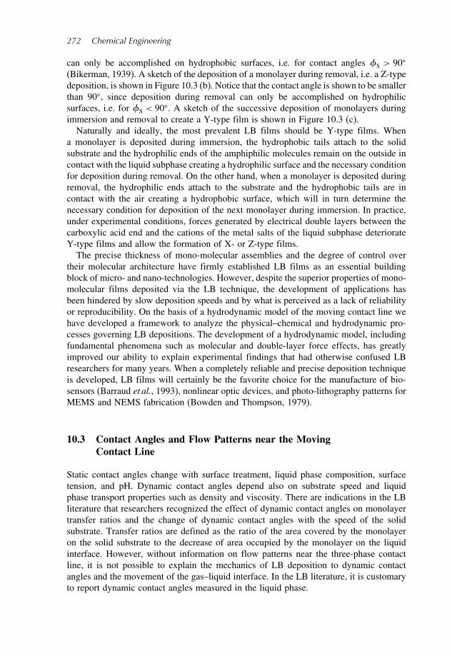
272 Chemical Engineering
can only be accomplished on hydrophobic surfaces, i.e. for contact angles S > 90
(Bikerman, 1939). A sketch of the deposition of a monolayer during removal, i.e. a Z-typedeposition, is shown in Figure 10.3 (b). Notice that the contact angle is shown to be smallerthan 90, since deposition during removal can only be accomplished on hydrophilicsurfaces, i.e. for S < 90. A sketch of the successive deposition of monolayers duringimmersion and removal to create a Y-type film is shown in Figure 10.3 (c).Naturally and ideally, the most prevalent LB films should be Y-type films. When
a monolayer is deposited during immersion, the hydrophobic tails attach to the solidsubstrate and the hydrophilic ends of the amphiphilic molecules remain on the outside incontact with the liquid subphase creating a hydrophilic surface and the necessary conditionfor deposition during removal. On the other hand, when a monolayer is deposited duringremoval, the hydrophilic ends attach to the substrate and the hydrophobic tails are incontact with the air creating a hydrophobic surface, which will in turn determine thenecessary condition for deposition of the next monolayer during immersion. In practice,under experimental conditions, forces generated by electrical double layers between thecarboxylic acid end and the cations of the metal salts of the liquid subphase deteriorateY-type films and allow the formation of X- or Z-type films.The precise thickness of mono-molecular assemblies and the degree of control over
their molecular architecture have firmly established LB films as an essential buildingblock of micro- and nano-technologies. However, despite the superior properties of mono-molecular films deposited via the LB technique, the development of applications hasbeen hindered by slow deposition speeds and by what is perceived as a lack of reliabilityor reproducibility. On the basis of a hydrodynamic model of the moving contact line wehave developed a framework to analyze the physical–chemical and hydrodynamic pro-cesses governing LB depositions. The development of a hydrodynamic model, includingfundamental phenomena such as molecular and double-layer force effects, has greatlyimproved our ability to explain experimental findings that had otherwise confused LBresearchers for many years. When a completely reliable and precise deposition techniqueis developed, LB films will certainly be the favorite choice for the manufacture of bio-sensors (Barraud et al., 1993), nonlinear optic devices, and photo-lithography patterns forMEMS and NEMS fabrication (Bowden and Thompson, 1979).
10.3 Contact Angles and Flow Patterns near the MovingContact Line
Static contact angles change with surface treatment, liquid phase composition, surfacetension, and pH. Dynamic contact angles depend also on substrate speed and liquidphase transport properties such as density and viscosity. There are indications in the LBliterature that researchers recognized the effect of dynamic contact angles on monolayertransfer ratios and the change of dynamic contact angles with the speed of the solidsubstrate. Transfer ratios are defined as the ratio of the area covered by the monolayeron the solid substrate to the decrease of area occupied by the monolayer on the liquidinterface. However, without information on flow patterns near the three-phase contactline, it is not possible to explain the mechanics of LB deposition to dynamic contactangles and the movement of the gas–liquid interface. In the LB literature, it is customaryto report dynamic contact angles measured in the liquid phase.

Langmuir–Blodgett Films: A Window to Nanotechnology 273
The role of contact angles in LB film deposition was outlined by Bikerman (1939)who recognized the need of hydrophobic surfaces, i.e. contact angles S ≥ 90 forsuccessful immersion deposition (X-type), and of hydrophilic surfaces, i.e. contact anglesS ≤ 90 for successful removal deposition (Y- or Z-type). Bikerman (1939) used asimple geometrical argument, essentially the zipper mechanism that has been acceptedas the basic deposition mechanism (Roberts, 1990).Gaines (1977) performed the first systematic study of dynamic contact angles during
the transfer of monolayers. Static contact angles were measured using the meniscus heightmethod on treated glass substrates. Typical immersion dynamic contact angles wereS ≈ 110 and greater. Typical removal contact angles were 20 ≤ S ≤ 60. However,with no information on the hydrodynamics of the three-phase contact line, there was nota mechanism to explain the effect of wetting on the mechanics of LB deposition.Petrov et al. (1980) analyzed the causes for the entrapment of water between the solid
substrate and the monolayer in Z-type depositions. This phenomenon has many commonfeatures with film thinning processes found during foam and emulsion breakdown andit is dependent on interfacial properties and on molecular interactions between the solidsubstrate and the monolayer. Petrov et al. (1980) measured the maximum speed of removalof the solid substrate before entrainment of a water layer and found it to be dependenton pH and ionic strength. There is no record in the publication of the measurement ofdynamic contact angles.An experimental demonstration that the effect of pH on transfer ratios can be explained
by the effect of pH on dynamic contact angles was provided by Aveyard et al. (1992) forsubstrata moving at constant deposition speeds.Peng et al. (1985) recognized the value of the dynamic contact angle as a useful
characterization and diagnostic tool and used a Wilhelmy plate technique to measuredynamic contact angles during multilayer deposition of lead stearates on mica substrates.Experimental results show clear trends of transfer ratio dependence with contact angles,including the interesting feature that transfer ratios during removal decrease with increas-ing dynamic contact angle.A remarkable analysis of the role of hydrodynamics in LB depositions was done by
de Gennes (1986). This analysis concerns only deposition during removal of the solidsubstrate. de Gennes recognizes that the only flow pattern that would allow Y-depositionis a split-ejection streamline in the liquid phase. However, he uses as a reference thework of Huh and Scriven (1971), but their hydrodynamic theory predicts a rolling motionin the liquid phase.Petrov and Petrov (1998) developed a molecular hydrodynamic theory of film deposi-
tion during removal. Their theory correctly assumes a flow pattern – which we identifiedas a split streamline – between the solid substrate and the monolayer in Figure 10.5 (c).This pattern is indeed the necessary pattern for successful deposition during removal, butit is not the only flow pattern for solid removal at all dynamic contact angles. Petrov andPetrov (1998) address the kinetics of water removal between the solid and the monolayerand the formation of wet or dry monolayers depending on the amount of water entrained.Zhang and Srinivasan (2001) performed a hydrodynamic analysis of water entrainment
based on the augmented version of the film evolution equation, where molecular forcesand Marangoni effects can be introduced.Contact angles and flow patterns are nothing but symptoms of the effect of highly
asymmetric molecular and structural force fields in the vicinity of a contact line. The solid

274 Chemical Engineering
substrate and the liquid phase are dense phases with large molecular concentrations, whilethe gas phase is essentially a void. In the wedge-like shape of the moving contact line,this asymmetric geometry gives rise to unbalanced surface forces that in turn translateinto shear stresses at the interface. Recently, Fuentes et al. (2005) have shown that dis-crepancies between experiments and the purely hydrodynamic contact line theory cannotbe explained without introducing molecular and structural forces within the proximalregion of the moving contact line.In a stable dynamic situation, the velocity of the contact line must match the velocity of
immersion, or removal, of the solid. In the classical hydrodynamic theory two parametersdetermine the dynamics of the moving contact line: (1) the dynamic contact angle, D,and (2) the ratio of viscosities of the two fluids, R = A/B (Huh and Scriven, 1971).The three basic flow patterns near a moving contact line are shown schematically inFigures 10.4 and 10.5. Figure 10.4 shows the flow patterns during immersion of thesolid substrate, while Figure 10.5 shows the flow patterns during removal. The first flowpatterns in Figure 10.5 (a)–(c) are the mirror image of the patterns occurring duringimmersion. An additional flow pattern is shown in Figure 10.5 that does not correspondto a moving contact line. It is the dip-coating flow pattern, Figure 10.5 (d), correspondingto very small or zero contact angles where a liquid film is continuously entrained withthe substrate during removal. Additional, more complicated transition patterns have beenpredicted theoretically (Diaz and Cerro, 2003), but the size of the vortex is too small forexperimental confirmation.At a moving or dynamic contact line, the contact angle is modified by stresses of hydro-
dynamic origin developed in fluid motion. We will assume that in a region very close, i.e.within 2mm of the contact line, the interface is a straight line and that the contact angle isthe dynamic contact angle. In general, one of the fluids has a rolling flow pattern, while theother fluid shows a splitting streamline. In the first flow pattern of the immersion sequence,
Flow patterns
Figure 10.4 Schematic representation of flow patterns near a moving contact line duringimmersion of a solid substrate into a pool of liquid. (a) Split-injection streamline in phase Band rolling pattern in phase A. (b) Transition flow pattern with motionless interface androlling motion in phases A and B. (c) Rolling motion in phase B and split-ejection streamlinein phase A

Langmuir–Blodgett Films: A Window to Nanotechnology 275
(a) (b) (c) (d)
Figure 10.5 Schematic representation of flow patterns near a moving contact line duringremoval of a solid substrate from a liquid pool. (a) Rolling motion in the liquid phase and split-injection streamline in the gas phase. (b) Transition flow pattern with motionless interface.(c) Split-ejection streamline in the liquid phase and rolling motion in the vapor phase. (d) Dip-coating flow pattern with stagnation point in the air–water interface and a liquid film entrainedon the solid surface
Figure 10.4 (a), there is a split-injection streamline in the liquid phase and the air–liquidinterfacemoves away from the contact line.The contact anglemeasured in the liquid phase ispurposely represented as a small contact angle, i.e.D < 90. The third pattern, Figure 10.4(c) shows a rolling pattern in the liquid phase and a split-ejection pattern in the gas phasesuch that the air–liquid interface moves toward the contact line. Notice that the contactangle is purposely represented as a large contact angle, D > 90. The intermediate pat-tern, shown in Figure 10.4 (b), is a transition pattern and the air–liquid interface is motion-less. The contact angle in this case is an intermediate value between the contact angles inFigure 10.4 (a) and (c), typically around 90. The first flow pattern in the liquid phase,Figure10.4 (a), is describedas a split-injection streamlinepattern to signify that the fluidnearthe contact line is being displaced by fluid coming from the bulk of the liquid phase. In thethird sketch, Figure 10.4 (c), the flow pattern in the gas phase is described as a split-ejectionstreamline to signify that the fluid near the contact line leaves along the splitting streamline.During removal, as shown in Figure 10.5 (a)–(c) the flow patterns are reversed and for smallcontact angles the liquid phase shows a split-ejection pattern, while for large contact anglesthe liquid phase is in a rolling motion.Experimental evidence of the occurrence of these flow patterns and quantitative depen-
dence with contact angles was provided by Savelski et al. (1995). During LB deposi-tions one of the fluids is always a liquid, predominantly water, and the other fluid isair. Viscosity ratios are small when the solid is immersed as shown in Figure 10.4,R=air/water ≈ 002 1. Similarly, viscosity ratios are large when the solid is removedfrom the water bath as shown in Figure 10.5, R= water/air ≈ 50 1.When a wetting solid is removed from the liquid phase, the flow pattern in the liquid
phase is the split-ejection streamline pattern shown in Figure 10.5 (c). The interfaceliquid–air moves toward the contact line and a Z-type LB deposition is possible. Duringremoval, transfer ratios of the monolayer show a strong dependence with the relative

276 Chemical Engineering
velocity of the interface that is also a strong function of the contact angle. When anon-wetting solid is removed from the liquid phase, the flow pattern is a rolling motion,the interface moves away from the contact line, and LB deposition is not possible.For a perfectly wetting system, i.e. for very small or zero contact angles, a continuous
film of liquid is entrained on the solid substrate, creating a dip-coating flow pattern. Thedip-coating pattern, Figure 10.5 (d), has a stagnation point on the gas–liquid interface.The liquid entrained on the solid surface comes from inside the liquid phase and thelower part of the interface moves away from the solid. Under these conditions, it hasbeen shown (Diaz and Cerro, 2004) that LB deposition cannot take place.The experimental results showing flow patterns versus contact angles were used to
configure a map of flow regions as a function of flow parameters, shown in Figure 10.6.The x-axis is dynamic contact angles, D, and the y-axis is the logarithm of the vis-cosity ratios, R = A/B. For the formulation of the hydrodynamic theory (Huh andScriven, 1971), dynamic contact angles are measured on the advancing fluid and canvary from perfect wetting, D = 0, to entrainment, D = . Following this convention,in Figure 10.6, contact angles are measured in the liquid phase during immersion andcontact angles are measured in the air phase during removal.Flow region I in Figure 10.6 corresponds to the flow pattern of Figure 10.4 (a) and
shows a split-injection streamline in the lower fluid (i.e. liquid) and rolling motion in theupper fluid (i.e. air). The lower part of region I, below the line R= 1, takes place duringimmersion of wetting solids, that is for smaller dynamic contact angles. Notice that inregion I, the interface is moving away from the contact line.Region II shows a split streamline in the air phase and rolling motion in the liquid
phase. This pattern is found when a non-wetting solid is immersed in a liquid or for largerimmersion speeds. The interface is moving toward the contact line. Region III correspond-ing to the flow pattern of Figure 10.4 (c), presents a split-ejection streamline in the liquid
100
10
1
0.1
0.01
0 90 180Dynamic contact angle
R =
vis
cosi
ty r
atio
IV III
I
II
Figure 10.6 Map of flow regions as a function of viscosity ratio, R = A/B, and dynamiccontact angle, D. The solid line is the locus of the motionless interface transition patternas predicted by the hydrodynamic theory (Huh and Scriven, 1971). The dashed line is theexperimental locus of transition patterns

Langmuir–Blodgett Films: A Window to Nanotechnology 277
phase and a rolling pattern in the air phase. Region III represents the typical flow patternduring removal of wetting solids, for small removal speeds. Notice that in region III theinterface moves toward the contact line. Region IV shows a split-injection streamline inthe air phase and a rolling motion in the liquid phase. This pattern is typical of the removalof a non-wetting solid from a liquid. The air–liquid interface moves away from thecontact line.The fuzzy line dividing regions I and IV from regions II and III is the locust of points
where a stagnant interface – flow pattern of Figure 10.4 (b) – is found. This is a transitionpattern and the fuzzy line is used to represent typical experimental uncertainty for a cleantwo-fluid system. The locus of the motionless interface is usually found for dynamiccontact angles near D ∼ 90. In practice, large dynamic contact angles typical of treatedsubstrata are more sensitive to movement of the contact line than clean surfaces andexhibit considerable advancing–receding hysteresis (Blake and Ruschak, 1997).The dependence of dynamic contact angles on moving contact line velocity has been
the subject of many experimental studies since this is an important parameter in high-speed coating. For an early review of experimental data on dynamic contact angles,refer to Dussan (1979). For more recent reviews on dynamic contact angles, refer to theexcellent contributions of Blake (Chapter 5) and Kistler (Chapter 6) in Berg (1993).When a solid is immersed into a liquid, such as in X-type film deposition, dynamic
contact angles increase with immersion speed. Because of contact angle hysteresis, thestatic contact angle is not uniquely defined. The static contact angle, S, regardlesswhether it can be determined experimentally, is a concept that results in the applicationof a variational principle, i.e. any change in contact angle results in an increase in theentropy of the system. The contact angle defined by the variational principle complieswith the definition of the thermodynamic static contact angle. The limit at vanishingr and contact line speed of the dynamic contact angle, D NCaNRe, depends on thedynamic variables. This limit, in general, is not equal to the thermodynamic static contactangle and depends on the movement history of the system and on the geometry of thesolid surface. At very low immersion speed, i.e. when Us ∼ 0, the contact angle measuredin the liquid phase approaches the static contact angle from above, D → S +,i.e. during immersion, contact angles are larger than static contact angles. When theimmersion velocity increases, the contact angle increases steadily until it reaches D ∼.In Figure 10.6 this is the right-end side of the map where a small air film would beentrained between the solid and the LB film and determines the maximum speed ofoperation of high-speed coating. The phenomena of air entrainment have been determinedexperimentally in high-speed coating situations (Gutoff and Kendrick, 1982), but it is nota problem encountered in LB deposition where coating speeds are very small.When the solid is removed from the liquid, as in Y-type deposition, the dynamic
contact angle measured on the liquid phase decreases steadily with increasing speed.At very low removal speeds, i.e. when Us ≈ 0, the contact angle approaches the staticcontact angle from below, D → S−S, i.e. during removal dynamic contact anglesare smaller than static contact angles. At increasing removal speeds, the dynamic contactangle decreases until D = 0. If one measures the contact angle in the advancing phase,then the contact angle D = . Notice that this is also the right-end side of Figure 10.6for viscosity ratios larger than 1. At this point, a thin film of liquid would be entrainedbetween the solid and the LB film. Water entrainment between the solid substrate andthe monolayer is one of the biggest challenges in LB deposition. The causes for this

278 Chemical Engineering
phenomenon have been explored experimentally (Petrov et al., 1980; Peterson et al., 1983;Srinivasan et al., 1988) and theoretically (de Gennes, 1986; Zhang and Srinivasan, 2001).If we further increase the removal speed, continuous entrainment of the liquid phase
develops into the dip-coating regime (Diaz and Cerro, 2004). During the dip-coatingregime, shown schematically in Figure 10.5 (d), a continuous liquid film is removed,attached to the solid, and there are steady stagnation streamlines in the liquid and gasphases, slightly above the level of the liquid surface. The streamline pattern for thedip-coating regime is a deformed 2D four-vortex pattern where the gas–liquid interfacemoves away from the contact line. This transition has been demonstrated experimentally(Diaz and Cerro, 2004).
10.4 Windows of Operation for Successful LB Deposition
The experimental results described in this section, linking flow patterns to dynamiccontact angles, can be used to define the windows of operation during LB depositions.A qualitative map of the windows of operation is shown in Figure 10.7. The ordinates ofthe map are immersion/removal speeds and the x-coordinates are static/dynamic contactangles. The values on the x-axis, i.e. for Us = 0, are static contact angles. The linesseparating the regions on the map are drawn under the assumption that the dynamic contactangles depart from the static contact angle (i.e. D = fNCaS; Gutoff and Kendrick,1982). At the typical speed of deposition of LB films, departure from static-advancing or
1.0
0.8
30° 60° 90° 120° 150°180°
0.6
0.4
0.2
–0.2
–0.4
–0.6
–0.8
–1.0
0US
10–3 m/s
V IV
I II
III
Figure 10.7 Sketch illustrating a qualitative picture of the windows of operation of theLB technique. Removal velocities are positive and immersion velocities are negative. Theshadowed regions determine regions where LB deposition is not possible

Langmuir–Blodgett Films: A Window to Nanotechnology 279
static-receding contact angles is very small. Negative substrate speeds indicate immersionwhere D ≥S, and positive substrate speeds denote removal of the solid substrate whereD ≤ S.The map lines and the values of contact angle and removal speeds must be taken only
approximately. The lines dividing the flow regions in Figure 10.6 were drawn as fuzzylines to highlight two facts: (1) It is difficult to measure with precision the dynamiccontact angle, in the region very close to the moving contact line. Even with our bestvideo images there is a +/−5 uncertainty. (2) There may be small variations in dynamiccontact angles due to the presence of the LB film. There is no comprehensive andsystematic experimental data on the limits for good coating conditions. This has been oneof the sources of great frustration to researchers in this area. By identifying the problemwe hope to focus experimental efforts on this topic.
10.4.1 Conditions for X-Type Depositions
Region I in Figure 10.7 is typical of flow patterns during immersion of solids on wettingliquids and corresponds to region I in Figure 10.6. At dynamic contact angles smallerthan D ≈ 95 the liquid phase shows a split-injection streamline and the interface movesaway from the contact line. This flow situation is typical of systems, such as glass andwater showing very small static contact angles. Thus, during immersion of a wettingsolid surface, such as glass in water, the flow pattern near the contact line shows asplit-injection streamline in the water phase, the interface moves away from the contactline, and X-type deposition is not possible. The cutoff value of D ≈ 95 for X-typedepositions determined by Gaines (1977) agrees with the dynamic contact angles showinga transition flow pattern, determined by Savelski et al. (1995). One must remember thatat low and even at intermediate removal speeds (Us<1cm/s) for clean substrata, thedynamic contact angle is essentially equal to the static-advancing contact angle.Region II in Figure 10.7 corresponds to region II of Figure 10.6. In region II, dynamic
contact angles are larger than approximately 95, the liquid phase is in a rolling motion,the interface moves toward the contact line, and deposition is possible. A glass surfacecan be treated to obtain static contact angles larger than 95. Gaines (1977) showed thatit is possible to deposit X-type LB films on treated, non-wetting glass surfaces.The interface moves toward the contact line at a speed that is not necessarily the same
as the velocity of the solid surface (Savelski et al., 1995). For dynamic contact anglesabout 95, the velocity of the interface is close to 0 because it is within the region wherethe transition flow pattern (Figure 10.4 (b)) is found. Under these conditions transferratios from the liquid interface to the solid surface can be very low. Honig (1973)recognized the effect of contact angles on transfer ratios and supplied a set of observationssummarized as follows: (a) the transfer ratio is constant in successive layers but not equalto 1, (b) the transfer ratio depends on the number of layers already deposited on thesolid, and (c) the transfer ratios are not equal for the upward or downward depositions.Some of these observations cannot be substantiated by later experiments of others nor ourown experiments and highlight the lack of a sound framework to relate transfer, contactangles, and flow patterns. For contact angles below 95, no deposition is possible duringthe downward stroke. For contact angles slightly larger than 95, the transfer ratio will besmall because the interface moves slower than the solid surface. For larger contact angles,i.e. 120, during the downward stroke the transfer ratio will approach unity because thespeed of the interface approaches the speed of the solid substrate.

280 Chemical Engineering
X-type films deposited on the downward stroke are hydrophilic because the hydropho-bic part of the fatty acid molecules is deposited on the solid surface. Similarly, Z-typefilms deposited on the upward stroke are hydrophobic because the hydrophilic end of themolecules is deposited on the substrate. Obviously, there is no reason for the resultingcontact angles to generate equivalent transfer ratios. Finally, contact angles on multilay-ered Y-type films depend not only on the type of hydrophilic or hydrophobic moleculeends but also on the number of layers on the composite film (Gaines, 1977).For low contact line speeds, i.e. Us → 0, the dynamic contact angle is close to the static-
advancing contact angle. There is a theoretical possibility that X-type LB monolayerscould be deposited on a solid where S < 95 if the immersion speed is large enough toincrease the dynamic contact angle. Further increasing the contact line speed may causethe dynamic contact angle to approach D → 2 and air entrainment will take place.For an air–water system, however, air entrainment will occur at speeds well above thetypical operation speeds of LB deposition.
10.4.2 Conditions for Y- and Z-Type Depositions
Region III in Figure 10.7 represents the typical flow patterns found during removal of non-wetting solids, i.e. when the dynamic contact angles measured in the liquid phase are largerthan 90/100. The liquid phase is in rolling motion and the interface moves away from thecontact line making deposition infeasible. Notice that dynamic contact angles measured inthe liquid phase decreasewith increasing removal speed. Thus, it is theoretically possible todeposit LB films on solids with static contact angles larger than 90 as long as the speed ofthe contact line results in dynamic contact angles smaller than 90.Region IV is the window of operation for successful deposition of Y-type films. The
flow pattern in this region is typical during removal of solids with dynamic contactangles 0<D ≤ 90.The split-ejection streamline is in the liquid phase and the interfacemoves toward the contact line. The interface, however, moves at a speed lower than theremoval velocity of the solid substrate. For contact angles closer to but smaller than 90,the flow approaches the transition profile (Figure 10.4 (b)) and the speed of the interfaceis nearly 0. As the contact angle decreases, the speed of the interface increases. Thus,transfer ratios during removal deposition are largely affected by contact angles. Petrovand Petrov (1998) incorrectly assumed that by maintaining a constant surface pressurea transfer ratio of unity follows. Constant surface pressure indicates the integrity of thefilm on top of the interface, but it does not assure that the solid and the interface moveat the same speed. The effect of contact angles on transfer ratios was demonstratedexperimentally by Sanassy and Evans (1993; Evans et al., 1994) and by Diaz and Cerro(2004) for a different system. These authors showed a sharp decline in transfer ratios fordynamic contact angles between ∼35 and 50, corresponding to static contact anglesbetween ∼65 and 80. Regardless of the large difference between static and dynamiccontact angles, since flow patterns evolve toward the motionless interface for increasingcontact angles, experimental transfer ratios decline from ∼100% to ∼0%.For very small dynamic contact angles, the liquid is not completely removed by the
split streamline and it is entrained between the film and the solid surface, creating what isknown as a wet LB film. Water trapped between the solid surface and the LB monolayerprevents adhesion and is a leading cause of monolayer instability. Petrov et al. (1980)sketched the flow pattern near the moving contact line. The flow pattern is the onedescribed here for region IV. The authors, however, reference Huh and Scriven (1971)
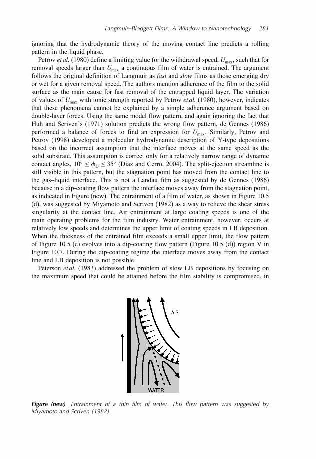
Langmuir–Blodgett Films: A Window to Nanotechnology 281
ignoring that the hydrodynamic theory of the moving contact line predicts a rollingpattern in the liquid phase.Petrov et al. (1980) define a limiting value for the withdrawal speed, Umax, such that for
removal speeds larger than Umax a continuous film of water is entrained. The argumentfollows the original definition of Langmuir as fast and slow films as those emerging dryor wet for a given removal speed. The authors mention adherence of the film to the solidsurface as the main cause for fast removal of the entrapped liquid layer. The variationof values of Umax with ionic strength reported by Petrov et al. (1980), however, indicatesthat these phenomena cannot be explained by a simple adherence argument based ondouble-layer forces. Using the same model flow pattern, and again ignoring the fact thatHuh and Scriven’s (1971) solution predicts the wrong flow pattern, de Gennes (1986)performed a balance of forces to find an expression for Umax. Similarly, Petrov andPetrov (1998) developed a molecular hydrodynamic description of Y-type depositionsbased on the incorrect assumption that the interface moves at the same speed as thesolid substrate. This assumption is correct only for a relatively narrow range of dynamiccontact angles, 10 ≤ D ≤ 35 (Diaz and Cerro, 2004). The split-ejection streamline isstill visible in this pattern, but the stagnation point has moved from the contact line tothe gas–liquid interface. This is not a Landau film as suggested by de Gennes (1986)because in a dip-coating flow pattern the interface moves away from the stagnation point,as indicated in Figure (new). The entrainment of a film of water, as shown in Figure 10.5(d), was suggested by Miyamoto and Scriven (1982) as a way to relieve the shear stresssingularity at the contact line. Air entrainment at large coating speeds is one of themain operating problems for the film industry. Water entrainment, however, occurs atrelatively low speeds and determines the upper limit of coating speeds in LB deposition.When the thickness of the entrained film exceeds a small upper limit, the flow patternof Figure 10.5 (c) evolves into a dip-coating flow pattern (Figure 10.5 (d)) region V inFigure 10.7. During the dip-coating regime the interface moves away from the contactline and LB deposition is not possible.Peterson et al. (1983) addressed the problem of slow LB depositions by focusing on
the maximum speed that could be attained before the film stability is compromised, in
Figure (new) Entrainment of a thin film of water. This flow pattern was suggested byMiyamoto and Scriven (1982)

282 Chemical Engineering
down- and upstrokes. The authors report the need for a hydrophobic surface in downstrokedeposition and the absence of a maximum speed limit. These findings are consistent withcontact line dynamics since larger immersion speeds increase the dynamic contact angle,the velocity of the interface approaches the velocity of the substrate, and consequentlytransfer ratios increase. The upper limit to this process, on the right-hand side of region II,would be entrainment of air. However, air entrainment would only occur at speeds muchlarger than the top speed of conventional Langmuir troughs. Interestingly, Peterson et al.(1983) report a lower limit for downstroke deposition (about 400m/s) which could betraced back to contact line instabilities. The effect of electrolytes (Petrov et al., 1980)and pH (Peng et al., 1985) on the maximum deposition speed during removal is anotherexample of how the dynamic of moving contact lines affects LB deposition and can betraced back to the flow transition to a dip-coating regime.Transfer ratio dependence with contact angle also determines the orientation of the films
deposited on the surface, as shown in Figure 10.3. Films deposited during downstrokehave the hydrophobic chain close to the solid, while films deposited during upstroke havetheir hydrophobic chains away from the solid surface, creating a headgroup to headgroupbilayer. The fact that some films rearrange after deposition to create the hydrophobic–hydrophobic and hydrophilic–hydrophilic arrangement has prompted some researchers topostulate the bilayer as the basic unit of an ideal LB film (Schwartz, 1997). One couldfurther speculate that the bilayer with external hydrophobic chains is the stable structureoutside the water subphase but the bilayer with external hydrophilic groups is the stablestructure inside the water subphase.
10.5 Marangoni Effects Due to the Presence of Langmuir Films
Transfer ratios for LB deposition during removal are largely affected by contact angles(Aveyard et al., 1992, 1995; Diaz and Cerro, 2004). The actual window for the high-efficiency deposition of LB films, i.e. transfer ratios near 100%, is relatively narrowand confined to a range of dynamic contact angles, 10≤ D ≤ 25. Within this region,however, the LB film plays a large role in stabilizing deposition from the gas–liquidinterface to the solid substrate.To demonstrate this effect an augmented version of the film evolution equation was
developed, introducing the disjoining pressure, , due to molecular forces as well asthe elasticity of the interface (Diaz and Cerro, 2003). The film evolution equation wasdeveloped for solving the pressure variable by integration of the component of themomentum balance, normal (Y direction) to the direction of flow (X direction). Theexpression for the pressure includes the capillary component, 2H, through surfacetension and surface curvature as well as the disjoining pressure computed on the basis ofmolecular and structural forces. The expression for pressure is subsequently substitutedinto the component of the momentum balance in the direction of flow and integratedacross the film thickness. To express this equation solely as a function of film thickness,HX, a generic velocity profile function, uXY , must be introduced. In our version ofthe film evolution equation, the velocity profile includes a shear stress source term at thegas–liquid interface that is computed as a function of molecular and structural forces andis part of the jump momentum balance at the interface. Additionally, this velocity profileverifies the conditions of non-slip at the solid surface and the conservation of mass, that

Langmuir–Blodgett Films: A Window to Nanotechnology 283
is, a constant net flow, Q. The resulting expression for the film evolution equation is asfollows:
d2H
dX= −d
dX+NBo+3Nca
(−12
u/Y Y=HX
HX− 1
HX2+ Q
HX3
)(10.2)
where Nca and NBo are the capillary and Bond number respectively that are defined as:
Nca =uw
0
NBo =gh2
0
begin the density of the liquid phase, u the bulk Newtonian viscosity, uw the liquidvelocity at the wall, 0 the surface tension of the pure liquid, of the gravity accelerationand h the thickness of the liquid film far from the liquid level at the bath.The disjoining pressure term is computed taking into account molecular, double
layer and structural forces as a function of the distance from the interface to the solidsurface.
=[
6∑m=4
(− m−3 m
HXm−2
)+ 3 sin
HX
]cos (10.3)
m=sm
Lm−2c
(10.4)
where angle is the angle between the interface and solid surface and m are functionsof the inclination angle for different values of m, the exponent of the binary interactionpotential.
m=−nLmLL Gm+nS
mSL
(Gm+Gm−
)(10.5)
where
G6=
12
(1+ 3
2cotcsc3
+ cos3)
G5=13sin cos+ −
G6−G6−=
6G5−G5−=
3(10.6)
and
G4= cos2(2
)G3=2 −
G4−G4−= G3−G3−= 2(10.7)
Finally at the air–water interface, the shear stress source term has two components
(U
Y
)
Y=HX
= Ts+(
X
)(10.8)

284 Chemical Engineering
The first component, Ts, is a resultant of molecular, double layer and structural forces onthe molecules at the air–water interface. The second component, /X, is due to theelasticity of the LB film at the interface and is written in dimensionless form
(
X
)= NEl
1US X
(US X
X
)(10.9)
where is the dimensionless interfacial tension = /uw, Us is the dimensionlessvelocity at the interface and the elasticity of the interface is defined as
NEl =(GL
lnA
)(1
UW
)(10.10)
The first term in equation 10.10 is the derivative of the interfacial tension with respectto the logarithm of the area occupied by the molecules, that is the negative of the slope ofthe surface pressure versus area per molecule given in Figure 10.2. The shear stress sourceterm is formulated using the jump momentum balance at the interface. For films withinthe solid region (Figure 10.2), the elasticity number is a very large number, typically105–106. Thus, when the interface is stretched due to fluid motion, a Marangoni-likeeffect creates a large force that pulls the interface up to the speed of the liquid interface.The resulting flow pattern is shown in Figure 10.8 (a). The velocity profile is a quadraticfunction of the coordinate normal to the movement of the solid, and an internal stagnationpoint develops as shown in Figure 10.8 (a). The streamline patterns computed using thefilm evolution equation are shown in Figure 10.8 (b). The interface velocity as a functionof vertical position is shown in Figure 10.8 (c). Notice that the velocity of the interface isremarkably constant and almost identical to the velocity of the solid substrate, indicatinga transfer ratio, TR ∼ 100%. For comparison we show also the velocity of a dip-coatingflow that would occur at the same capillary number.Even at the peak of the shear stress source term, these are of the order of 10−2 Pa.
Thus, outside of a certain range of contact angles, hydrodynamic forces are larger thanthe forces generated by the stretching of the film at the interface, despite the large valueof the elasticity number, and the interface velocity is smaller than the velocity of the solidsurface, resulting in transfer ratios smaller than 100%. Figure 10.9 shows the values ofexperimental transfer ratios of zinc arachidate films for different dynamic contact angles.Subphase temperature was kept at 26C, stroke speed was 19mm/min, concentration ofthe spreading solution was 1mg/mL of arachidic acid in chloroform, concentration of thesubphase was 10−4 M of ZnSO4, and surface pressure was 25mN/m. Surface treatmentof the solid substrate and pH were varied in order to cover a wide range of valuesof dynamic contact angles. Figure 10.9 shows transfer ratios for clean glass slides andglass slides coated with diluted Sigmacote® during upstrokes at pH = 53 as a functionof dynamic contact angles. The largest transfer ratios during upstroke are obtained fordynamic contact angles of about 10– 25 using clean glass slides at pH = 53. In thisregion the transfer ratios are close to 100%. For these range of contact angles the liquidsubphase flows in a split-ejection flow pattern and the interface moves toward the solidat a velocity close or equal to the velocity of withdrawal of the solid substrate. Asthe contact angle is increased, by using glass slides treated to become only partiallywetting, the transfer ratio decreases. The transfer ratio decreases with increased contactangles because the velocity of the air–liquid interface decreases steadily until it becomes

Langmuir–Blodgett Films: A Window to Nanotechnology 285
x (m
m)
y (mm)
h (µm)
Us
Figure 10.8 Flow pattern during removal–deposition of an LB film. NCa =1.90.10−5 andNEl =4.01.105. (a) Schematic representation; (b) computation results for the streamlines;(c) relative interface velocity (solid line) and relative dip coating velocity (dashed line) versusthe film thickness
0 near 90. At this point the split-ejection flow pattern (Figure 10.5 (c)) evolves intothe transition flow pattern (Figure 10.5 (b)). Further increase in dynamic contact anglepromotes a transition to the rolling flow pattern in the liquid subphase and the transferratio is 0. These results agree very well with experimental data presented by Evansand coworkers (Sanassy and Evans, 1993; Evans et al., 1994) for gold-coated substratesimmersed in mixture thiols, and using pure water as the liquid subphase.Using clean glass slides only, pH was increased in several steps adding a dilute
solution of ammonium hydroxide to the 10−4 M zinc sulfate subphase. A monolayerof arachidic acid is partially ionized at pH = 53. Increasing the pH of the subphase to6.6 and 7.7 causes an increase of ionization of the carboxylic headgroups. At higherpH, the monolayer is completely ionized. No area loss of monolayer is observed overthe experimental period for all the values of pH. Transfer ratios at pH 6.6 and 7.7 areessentially the same as at pH = 53, that is, close to 100%. However, when pH reaches8.7, the dynamic contact angle is very small or 0 and no transference of monolayer tothe solid substrate is recorded while it is evident that a thin film of liquid leaves with thesolid substrate. Similar results were obtained for pH 9.4, 10.1, and 10.6. These resultsare shown on the left-end side of Figure 10.9.

286 Chemical Engineering
Angle (degrees)
Tra
nsfe
r ra
tio (
%)
Figure 10.9 Experimental transfer ratios (TR) versus dynamic contact angles duringupstrokes for different pH values. Open squares: Sanassy and Evans (1993) results withpure water. Results from this work: deposition were made at surface pressure of 25mN/m,T= 26 C and a deposition speed of 19mm/min. The values of the pH were as follows:pH=5.3 (diamonds); pH=6.6 (star); pH=7.7 (cross); pH=8.7 (open circle); pH=9.4(asterisk); pH=10.1 (×); pH=10.6 (open triangle). The line is just a guide to the eye
During immersion a hydrophobic surface, i.e. a large contact angle between the liquidand the solid surface, is needed for successful LB depositions. Downstroke experi-ments were performed using glass slides coated with diluted Sigmacote® and with ferricstearate to create dynamic contact angles larger than 90. All experiments were done at26C65mm/min stroke velocity, and pH = 53. These experimental results are shownin Figure 10.10. At dynamic contact angles ranging from 50 to 90 transfer ratios areessentially 0 because the flow pattern in the liquid subphase shows a split-injectionstreamline with the interface moving away from the contact line. Under these conditions,no LB deposition is possible. For dynamic contact angles between 120 and 130 transferratios are essentially 100%. For large dynamic contact angles the flow pattern in theliquid subphase is a rolling motion and deposition is possible. It is not clear why duringdownstroke transfer ratios go from 0 to 100% with no apparent intermediate values.The argument that monolayer compression promotes the movement of the interface, asthe compressing barriers move in, is unlikely because this effect is not apparent duringupstroke where the transition from an interface moving with the speed of the solid sub-strate to a motionless interface occurs smoothly as the dynamic contact angle increases(Figure 10.9), regardless of the pressure applied on the monolayer. We were unable to

Langmuir–Blodgett Films: A Window to Nanotechnology 287
Tra
nsfe
r ra
tio (
%)
Angle (degrees)
Figure 10.10 Experimental transfer ratios (TR) versus dynamic contact angles during down-strokes for different pH values. The conditions of deposition were as follows: a surfacepressure of 25mN/m, 26 C, and a deposition speed of 19mm/min. The values of the pHwere as follows: pH=5.3 (diamonds); pH=6.6 (star); pH=7.7 (cross); pH=8.7 (opencircle); pH=9.4 (asterisk); pH=10.1 (×); pH=10.6 (open triangle). The line is just a guideto the eye
create surfaces with contact angles ranging from 90 to 120, thus it is not possible todetermine if, within this range, there is a smooth variation from 0 transfer ratios to 100%.
10.6 Role of Molecular, Structural, and ElectricalDouble-Layer Forces
Short-range molecular forces, i.e. with ranges up to 3 nm, can account for a varietyof macroscopic phenomena. Short-range molecular forces account for capillarity, theshapes of macroscopic liquid droplets on surfaces, the contact angle between coalescingsoap bubbles, and the breakup of a jet of water into spherical droplets (Israelachvili,1985). Long-range structural forces, namely hydrophobic forces, can be accounted for atdistances as long as 300 nm (Colic and Miller, 2000). Electrostatic double-layer forcescontrol the macroscopic properties of slurries and cause large differences in pressure dropduring slurry filtration. The recognition that long-range structural forces are significantbeyond tens and hundreds of molecular diameters allowed the explanation of macroscopic

288 Chemical Engineering
phenomena such as capillarity, the stability of colloidal and particle suspensions, and thebreakup of liquid films on solid surfaces (Derjaguin et al., 1987).Independently and almost simultaneously the effect of molecular forces near a three-
phase contact line was analyzed by Miller and Ruckenstein (1974) and Jameson andGarcia del Cerro (1976). While both papers point to the presence of asymmetric forcefields, mainly generated by the presence of two dense phases (solid and liquid) and agas phase, Miller and Ruckenstein (1974) developed the concept of a resulting forceto explain the movement of a contact line and Jameson and Garcia del Cerro (1976)balanced the resultant force with an interfacial tension gradient.The need to introduce molecular and structural forces to explain flow patterns near
a moving contact line was recently recognized (Fuentes et al., 2005) and flow patternsnear moving contact lines have been used to explain the windows of operation of LBdepositions (Cerro, 2003). When a contact line moves, unbalanced molecular and struc-tural forces produce a residual shear stress at the solid–liquid and fluid–fluid interface.In the presence of surfactants or contaminants at the interface, motion can generateMarangoni-like effects due to changes in surface concentration. On clean interfaces anelasticity component results, from stretching and compressing the interface (Edwardset al., 1991). Thus, it is generally accepted that, regardless of the source, there is a strongforce asymmetry at the contact line.Unlike colloidal particles, moving contact lines are inherently asymmetric. Electrical
potentials of double layers in a solid–liquid interface can be different in magnitude andin sign to the potentials of the air–liquid interface on the same liquid pool. Thus, wemay have attractive or repelling forces at the contact line, depending on the nature of theinterfaces and on the pH of the liquid phase. The nature and the effect of these forcesand their effect on contact angles have been analyzed (Churaev, 1995).The interaction of the double layers near the moving contact line and its effect on
LB depositions, has been recognized (Petrov, 1986) but the connection between doublelayers and flow patterns has not been explored until recently (Fuentes et al., 2005). Wedevelop here a framework for analyzing the hydrodynamics of LB depositions under thepresence of electrical double layers on the solid–liquid interface and on the air–liquidinterface. These interfaces are subject to movement, the motion disrupts the diffusionlayer, essentially creating streaming potentials. In addition, both interfaces show a largeconcentration of charged molecules, behaving essentially as 2D solids.In general, when two phases are in contact, electrons or ions will be attracted in
different ways by the different phases and dipolar molecules will be oriented selectively(Hunter et al., 1981). When a solid phase is in contact with a liquid subphase the solidsurface may be charged and surrounded by ions of opposite sign (counterions). This is thetypical arrangement of an electrical double layer as described by the Gouy–Chapman–Grahame–Overbeek theory of potential and charge distributions in electrical doublelayers (Grahame, 1947; Overbeek, 1952). In LB depositions, there are two interfaces thatacquire charge, the substrate–subphase interface and the LB film–subphase interface. Thesubstrate–subphase interface is a typical solid–liquid interface with the difference thatit may or may not have a deposit consisting of one or many layers of the amphiphiliccompound that makes up the LB film. For short, we will call this surface the solid–liquidinterface. The LB film–subphase is for all purposes also a solid–liquid interface, with onelayer of the amphiphilic compound compressed to the point that is essentially a 2D solid.We will denote this as the film–liquid interface. At the contact line, that is, the line where

Langmuir–Blodgett Films: A Window to Nanotechnology 289
the three phases coincide, the double layers of the solid–liquid and film–liquid interfacesoverlap. The sign and magnitude of the electrical forces created by the presence of theelectrical double layers determine the dynamic contact angle and the flow patterns neara moving contact line.At least two of the recognized mechanisms for the formation of electrical double
layers (Hunter, et al. 1981; Russel et al., 1989) are relevant to LB film depositions:(1) ionization of carboxylic acid group and amphoteric acid groups on solid surfaces,and (2) differences between the affinities of two phases for ions or ionizable species.The latter mechanism includes the uneven distribution of anions and cations betweentwo immiscible phases, the differential adsorption of ions from an electrolyte solutionto a solid surface, and the differential solution of one ion over the other from a crystallattice. Since the solid–liquid and the film–liquid interfaces are flat, large surfaces andsince both have a large, solid-like concentration, the analysis that follows applies to bothinterfaces. For an interface conformed by a thin film of an amphiphilic compound withthe hydrophilic end of the molecule in contact with the water subphase, the equilibriumof charges is based on pH and subphase concentration. The effect of pH is highlightedby the definition of the pKa of the carboxylic acid:
H2O+RCOOH RCOO−+ H3O+ (10.11)
The equilibrium constant for this reversible ionization process is written in terms of ionicconcentrations:
Keq =H3O
+ RCOO−
RCOOH H2O(10.12)
By definition, pKa is the pH when the concentration of ionized carboxylic acid is equalto the concentration of non-ionized acid groups:
Ka =H3O
+
H2O pKa = pH (10.13)
where pKa is equal to the pH only when half of the carboxylic acids are ionized. Valuesof pKa depend on the length of the hydrocarbon chain attached to the carboxylic groupand are also mildly modified by the presence of a metal subphase counterion and itsmatching group. When an amphiphilic carboxylic acid and its subphase are at the pKa, theintermolecular distances between molecules at the air–water interface reach a minimum(Kanicky et al., 2000) and macroscopic properties, such as foam height and stability aswell as surface viscosity, are at a maximum value. The ion–dipole interactions takingplace between ionized and non-ionized carboxylic groups are somehow complementedby the presence of divalent cations in the liquid subphase (i.e. Cd++Zn++, etc). There isexperimental evidence that monovalent (i.e. NH+
4 ) or trivalent (i.e. Fe+++) cations have
very different effects on monolayer stability (Gaines, 1966).Although the theoretical tools for modelling and interpreting double-layer properties
and electrokinetic behavior have been around for a long time (Kruyt, 1952), it was notuntil recently that -potentials and electrokinetic properties could be measured accurately(Gu and Li, 2000; Usui and Healy, 2002). Regardless of the particular charge of theLB film and of the thickness of the electrical double layer, the following facts must

290 Chemical Engineering
be stressed: (1) the thickness of the electrical double layer, i.e. the width of the regionwhere the electrical potential decays to within 2% of its maximum value, is of the sameorder of magnitude as the size of the proximal region (de Gennes et al., 1990) in thedescription of moving contact lines; (2) the sign and magnitude of the charge at thesolid–liquid and the film–liquid interfaces depend on pH and subphase salt concentration;and (3) the relative movement of liquid with respect to the solid substrate, due to theimmersion/removal of the solid surface and to the movement of the mechanical barriersto compress the LB film, affects the integrity of the double layer and creates a streamingpotential.The thickness of the electrical double layer can be estimated in tens and perhaps
hundreds of nanometers. When the solid–liquid and film–liquid interfaces approach thethree-phase contact line, the double layers overlap and interact. This interaction leadsto attraction–repulsion forces that determine contact angles (Churaev, 1995) and flowpatterns (Fuentes et al., 2005) near the moving contact line. Flow patterns, in turn, havebeen linked to the ability to deposit an LB film on a moving substrate (Cerro, 2003).Double-layer sign and magnitude of the charge depend on subphase pH and concentrationof the metal salts in the subphase. During successive deposition of LB films, the samecompound is deposited on the solid–liquid and film–liquid interfaces. If the liquid sub-phase is at the pKa of the carboxylic acid, interaction between ionized and non–ionizedacid groups keeps the film at a relatively small charge level. Experimental measurementsof -potential of stearic acid films (Usui and Healy, 2002) show at pKa = 48 neg-ative charges, V = −80mV, smaller than the maximum value of V = −150mV, atpH∼ 85. It is important to point out that these measurements were made for stearic acidlayers in the presence of NH4NO3–NH4OH subphases, i.e. for a monovalent ion.Carboxylic acid films in the solid–liquid or in the film–liquid interface submerged
in the same water subphase should develop a similar type of double layer, with similarsign and magnitude of charge. Thus, during immersion the hydrophobic hydrocarbonchains can account for a large contact angle, allowing deposition, but during removal thecarboxylic acid ends will have same sign charges creating repulsion and a large contactangle, preventing LB deposition. Consequently, a Y to X film transition arises becausedeposition during removal cannot take place.In addition, immersion and removal speeds play a definite role in LB depositions
because they disturb equilibrium of charges at the electrical double layer. When thesolid is immersed, the double layer begins to form and ions must diffuse toward andaway from the solid surface before equilibrium is reached. When the solid is removed,the double layer is partially wiped out by the flow but metal cations are retained onthe film deposited on the solid substrate. On the other hand, during film deposition, themechanical barriers designed to keep the surface pressure constant move the film on theair–water interface and disturb the double layers under the film. At this point, we do nothave a quantitative way to estimate the disturbance to the double layer caused by themovement of the solid substrate, but we can introduce the following assumptions:
(1) The movement of the substrate disturbs the double layer and generates a streamingpotential.
(2) The streaming potential drives a streaming current in the reverse direction to restorecharges and approach equilibrium.

Langmuir–Blodgett Films: A Window to Nanotechnology 291
(3) The magnitude of the streaming potential and the streaming currents are directlyproportional to the -potential of the double layer and to the velocity of the solidsubstrate (Gu and Li, 2000).
(4) The dynamics of double-layer formation are controlled by the electrokinetic velocityof ions and it takes a certain amount of time for the double layer to re-establish.
Taking into account what we know about electrical double layers and their effect ondynamic contact angles and flow patterns, we attempt an explanation of Y to X filmtransitions, on the basis of our experimental data. Figure 10.11 shows deposition ofsuccessive layers of arachidic acid at a pH equal to the pKa = 55 of arachidic acid.Subphase is a solution of CdCl2 at 2.0 10−4 M and glass slides treated with ferric stearatewere immersed and removed at constant speed, Us = 60mm/min, and a constant sur-face pressure of = 25mN/m. Contact angles were consistently low, about 30 duringremoval, and consistently high, about 110 during immersion, assuring successful depo-sition for at least 18 monolayers without apparent change in deposition effectiveness.Figure 10.12 shows similar experiments with identical substrate and subphase conditionsbut for a different pH = 61. Clearly, deposition during immersion remains high, andcontact angles, not shown in the figure, remain over 100. Contact angles during removalare small for the first three cycles but they soon reach values of the order of 60–70,and deposition during removal stops.
120
100
80
60
40
20
00 2 4 6 8 10 12 14 16 18
0
50
100
150
200
205A
ngle
(de
gree
s)
Tra
nsfe
r ra
tio (
%)
Layer number
Figure 10.11 Variation of transfer ratio and dynamic contact angle with number of layers forthe deposition of arachidic acid on a subphase of 2.10−4 M CdCl2 at pH=5.5, =25mN/m,60mm/min, and T= 25C. Squares and solid lines: transfer ratios; diamonds: dynamic contactangles

292 Chemical Engineering
0
0 2 4 6 8 10 12 14 16
150
100
50
0
Ang
le (
degr
ees)
120
100
80
60
40
20
Tra
nsfe
r ra
tio (
%)
Layer number
Figure 10.12 Variation of transfer ratio and dynamic contact angle with layer number forthe deposition of arachidic acid on a subphase of 2.10−4 M CdCl2 at pH=6.1, =25mN/m,60mm/min, and T = 25 C. Squares and solid lines: transfer ratios; diamonds: dynamiccontact angles
120
140
100
80
60
40
20
Tra
nsfe
r ra
tio (
%)
Layer number2 4 6 8 10 12 14 16 18
Figure 10.13 Variation of transfer ratio with layer number for the deposition of arachidicacid on a subphase of 2.10−4 MCdCl2 at pH=5.7, =25mN/m, and T= 25 C. Dotted line:60mm/min; dashed-dotted line: 15mm/min; dashed line: 9mm/min; solid line: 3mm/min

Langmuir–Blodgett Films: A Window to Nanotechnology 293
Figure 10.13 shows successive deposition of films of arachidic acid at pH= pKa = 55at different removal speeds. Experiments were done with identical glass slides treated withferric arachidate, and similar subphase concentrations of CdCl2 of 10
−4 M. The removalspeeds were 3, 9, 15, and 60mm/min. Notice that successive depositions at 15 and60mm/min show transfer ratios close to 100%. Depositions at 9mm/min show signs ofdecreasing transfer ratios after 10 layers. However, at 3mm/min transition from Y to Xfilms takes place after a couple of cycles. Assuming that the immersion/removal cyclestake place without stopping at the higher and lower positions of the substrate, and thatthe length of the substrate run is 20mm, the times elapsed for one cycle are 13.3, 4.4,2.6, and 0.6min for the 3, 9, 15, and 60mm/min substrate speeds. To test the premisethat electrokinetic effects determine the speed at which the double layer is being restored,slides were let to rest inside the liquid subphase for a period of 10min after immersion.Experimental results allowing the substrate to equilibrate for 10min inside the liquidsubphase are shown in Figure 10.14. Notice that deposition of LB films during removalfor films left to age under the liquid subphase is affected in a way similar to the lowerdeposition speed shown to be affected in Figure 10.13.On the basis of experimental evidence and taking into account the role of electrical
double layers on contact angles and flow patterns, one can certainly argue that the mostsuccessful conditions for multilayer Y-type LB deposition take place at a pH equal tothe pKa of the carboxylic acid, with a subphase where a minimum concentration of a
120
100
80
60
40
20
02 4 6 8 10 12
Layer number
Tra
nsfe
r ra
tio (
%)
14 16 18
Figure 10.14 Variation of transfer ratio with layer number for the deposition of arachidicacid on a subphase of 2.10−4 MCdCl2 at pH=5.7, =25mN/m, and T= 25 C. Solid line:64mm/min; dotted line: 64mm/min, and held under water for 10min

294 Chemical Engineering
divalent cation is available, at deposition velocities large enough to perturb the electricaldouble layer and with short time exposure under the liquid. The role of the pH = pKa
and the presence of a divalent cation, although not well understood, indicate a certainamount of a crystal-like structure in LB films. Atomic force microscopy images of LBfilms deposited on all kinds of solid surfaces (Zasadinsky et al., 1994) show that themain requirement for long-range order in the alkyl chains is to have an underlyingheadgroup to headgroup interface. This fact may also explain why transition from Y- toX-type depositions occurs only at or after the second cycle (Figure 10.12). Stripe-shapedridges on films of metal salt arachidates have been explained on the basis of orderedpatterns of ionized or salt-forming carboxylic headgroups and non-ionized headgroups(Sigiyama et al., 1998).
10.7 Conclusions
The experiments described in this chapter and the concepts put forward to explain theseexperiments are an attempt to understand the mechanics of LB depositions, a largeand fascinating scientific problem. There should be no doubt that flow patterns and therelative movement of the air–water interface determine feasibility of LB deposition. TheMarangoni-like effects generated by the stretching of the film on the interface help tocreate a region for high transfer ratios by controlling, within certain limits, the velocity ofthe interface. One must remember though that one-molecule-wide films cannot supportstresses substantial enough to change qualitatively the flow patterns near the movingcontact line. However, electrical double layers on the film at the air–water interfaceand similar double layers surrounding the films deposited on the solid substrate createattraction/repulsion effects that determine contact angles and flow patterns.The movement of the solid substrate and the movement of the film at the air–water
interface due to the pressure-controlling barriers create disturbances in the electricaldouble layers that allow deposition of multiple LB films. This is a novel way to lookat the LB technique and puts multilayer depositions under a totally new light. Electricaldouble layers can be modified in a number of chemical, electrical, and mechanical waysto enhance depositions, opening a wide range of alternatives for the development ofmultilayer deposition techniques.There are many questions remaining and many puzzling, unexplained effects such as
the effect of cation size and valence on film stability. These questions point to the needto develop a better understanding of the crystal-like structure of LB films, the role ofmolecular and structural forces in creating these structures, and the nature and stability ofelectrical double layers subject to mechanical perturbations in the underlying subphase.There is also a growing need to develop characterization techniques that can be
applied, in situ, during deposition and would allow determination of film structure,charge, and electrical double-layer characteristics. The transfer ratio is a crude andsometimes misleading method of characterization but unfortunately, in this aspect, wehave not advanced far past Katherine Blodgett’s primitive experiments. Brewster anglemicroscopy (BAM), atomic force microscopy (AFM), and attenuated total reflectanceinfrared spectroscopy (ATR) are some of the emerging techniques that may help to bridgethis gap as they become standard instrumentation associated with LB troughs.
Langmuir–Blodgett Films: A Window to Nanotechnology 295
The applications of LB films are far reaching. Highly ordered LB films have manyinteresting properties, but more important than their technological applications is the factthat these films hold the key to nature’s molecular world where order is essential tofunction.
10.8 Summary
The transfer onto the surface of a solid substrate of successive monolayers of divalentsoaps compressed on the surface of water in a Langmuir trough was described byBlodgett (Blodgett, 1935). A Langmuir trough is a container with moving barriers formanipulation of a film of an amphiphilic compound at the air–water interface. Films aredeposited on solid substrata moved up and down, out and into the water subphase. Theterm Langmuir–Blodgett (LB) technique is currently used to denote the deposition ofmonolayers by transfer from the air–water interface onto a solid surface.Single, i.e. one-layer, LB films show a remarkable ordered structure. The precise
thickness of mono-molecular assemblies and the degree of control over their moleculararchitecture have firmly established LB films in ultrathin film technology as an essentialbuilding block of micro- and nano-technologies.
Acknowledgements
The research work that provided the foundations of this article was supported by grantCTS-0002150 of the National Science Foundation.
References
Aveyard R., Binks B.P., Fletcher P.D.I. and Ye X. 1992. Dynamic contact angles and depositionefficiency for transfer of docosanoic acid onto mica from CdCl2 subphases as a function of pH,Thin Solid Films, 210, 36–38.
Aveyard R., Binks B.P., Fletcher P.D.I. and Ye X. 1995. Contact angles and transfer ratios measuredduring the Langmuir–Blodgett deposition of docosanoic acid onto mica from CdCl2 subphases,Colloid Surf., A: Physicochem. Eng. Aspects, 94, 279–289.
Barraud A., Perrot H., Billard V., Martelet C. and Therasse J. 1993. Study of immunoglobulin Gthin layers obtained by the LB method: application to immunosensors, Biosens. Bioelectron., 8,39–48.
Berg J.C. (Ed.). 1993. Wettability. Surfactant Science Series. Marcel Dekker, New York.Bikerman J.J. 1939. On the formation and structure of multilayers, Proc. R. Soc. Lond. A Math.
Phys. Sci., 170, 130–144.Blake T.D. and Ruschak K.J. 1997. Wetting: static and dynamic contact lines. In, Liquid Film
Coating. Scientific Principles and their Technological Implications, Kistler S.F. and SchweizerP.M. (Eds.). Chapman & Hall, New York, pp. 63–97.
Blodgett K.B. 1935. Films built by depositing successive monomolecular layers on a solid surface,J. Am. Chem. Soc., 57, 1007–1022.
Bowden M.J. and Thompson L.F. 1979. Resists for fine line lithography, Solid State Technol.,22(5), 72–82.

296 Chemical Engineering
Cerro R.L. 2003. Moving contact lines and Langmuir–Blodgett film deposition, J. Colloid InterfaceSci., 257, 276–283.
Churaev N.V. 1995. The relation between colloid stability and wetting, J. Colloid Interface Sci.,172, 479–484.
Colic M. and Miller J.D. 2000. The significance of interfacial water structure in colloidal systems –dynamic aspects. In, Interfacial Dynamics, Vol. 88, Kallay N. (Ed.), Marcel Dekker, New York.
Derjaguin B.V., Churaev N.V. and Muller V.M. 1987. Surface Forces. Plenum Press, New York.Diaz E. and Cerro R.L. 2003. Flow Bifurcation during Removal of a Solid from a Liquid Pool.
AIChE Annual Meeting, San Francisco, CA.Diaz M.E. and Cerro R.L. 2004. Transition from split streamline to dip-coating during Langmuir–
Blodgett film deposition, Thin Solid Films, 460, 274–278.Dussan V E.B. 1979. On the spreading of liquids on solid surfaces: static and dynamic contact
angles, Annu. Rev. Fluid Mech., 11, 371–400.Edwards D.A., Brernner H. and Wasan D.T. 1991. Interfacial Transport Processes and Rheology.
Butterworth-Heinemann, Boston.Elliot D.J., Furlong D.N. and Grieser F. 1999. Formation of CdS and HgS nanoparticles in LB
films, Colloid. Surface., 155, 101–110.Evans S.D., Sanassy P. and Ulman A. 1994. Mixed alkanethiolate monolayers as substrates for
studying the Langmuir deposition process, Thin Solid Films, 243, 325–329.Fuentes J., Savage M. and Cerro R.L. 2005. On the effect of molecular forces on moving contact
lines, J. Fluid Mech. (submitted).Gaines G.L. 1966. Insoluble Monolayers at the Gas Liquid Interfaces. John Wiley & Sons,
New York.Gaines G.L. 1977. Contact angles during monolayer deposition, J. Colloid Interface Sci., 59,
438–446.de Gennes P.G. 1986. Deposition of Langmuir–Blodgett layers, Colloid Polym. Sci., 264, 463–465.de Gennes P.G., Hua X. and Levinson P. 1990. Dynamics of wetting: local contact angles, J. Fluid
Mech., 212, 55–63.Grahame D.C. 1947. The electrical double layer and the theory of electrocapillarity, Chem. Rev.,
41, 441–501.Gu Y. and Li D. 2000. The potential of glass surface in contact with aqueous solutions, J. Colloid
Interface Sci., 226, 328–339.Gutoff E.B. and Kendrick C.E. 1982. Dynamic contact angles, AIChE J., 28, 459–466.Honig E.P. 1973. Langmuir–Blodgett deposition ratios, J. Colloid Interface Sci., 45, 92–102.Huh C. and Scriven L.E. 1971. Hydrodynamic model of the steady movement of a solid/liquid/fluid
contact line, J. Colloid Interface Sci., 35, 85–101.Hunter R.J., Ottewill R.H. and Rowell R.L. 1981. Zeta Potential in Colloid Science. Academic
Press, London.Israelachvili J.N. 1985. Intermolecular and Surface Forces. Academic Press, London.Jameson G.J. and Garcia del Cerro M.C. 1976. Theory for the equilibrium contact angle between
a gas, a liquid, and a solid, Trans. Faraday Soc., 72, 883–895.Kanicky J.R., Poniatowski A.F., Mehta N.R. and Shah D.O. 2000. Cooperativity among molecules
at interfaces in relation to various technological processes: effect of chain length on the pKa offatty acid salt solutions, Langmuir, 16, 172–177.
Keller D.J., Korb J.P. and McConnell H.M. 1987. Theory of shape transitions in two-dimensionalphospholipid domains, J. Phys. Chem., 91, 6417–6422.
Kruyt H.R. (Ed.). 1952. Colloid Science. Elsevier Publishing, Amsterdam.Miller C.A. and Ruckenstein E. 1974. The origin of flow during wetting of solids, J. Colloid
Interface Sci., 48, 368–373.Miyamoto K. and Scriven L.E. 1982. Breakdown of Air Film Entrainment by Liquid Coated on
Web. AIChE Annual Meeting.

Langmuir–Blodgett Films: A Window to Nanotechnology 297
Overbeek J.T.G. 1952. Electrochemistry of the double layer. In, Colloid Science, Kruyt H.R. (Ed.),Vol. 1. Elsevier Publishing, pp. 115–193.
Peng J.B., Abraham B.M., Dutta P. and Ketterson J.B. 1985. Contact angle of lead stearate-coveredwater on mica during the deposition of LB assemblies, Thin Solid Films, 134, 187–193.
Peterson I.R. 1996. Langmuir–Blodgett Techniques. Marcel Dekker, New York.Peterson I.R., Russell G.J. and Roberts G.G. 1983. A new model for the deposition of w-tricosenoic
acid LB film layers, Thin Solid Films, 109, 371–378.Petrov J.G. 1986. Dependence of the maximum speed of wetting on the interactions in the three-
phase contact zone, Colloids Surf., 17, 283–294.Petrov J.G., Kuhn H. and Mobius D. 1980. Three-phase contact line motion in the deposition of
spread monolayers, J. Colloid Interface Sci., 73, 66–75.Petrov J.G. and Petrov P.G. 1998. Molecular hydrodynamic description of Langmuir–Blodgett
deposition, Langmuir, 14, 2490–2496.Roberts G.G. (Ed.) 1990. Langmuir–Blodgett Films. Plenum Press, New York.Roth K.M., Rajeev N.D., Dabke B., Gryko D.T., Clausen C., Lindsey J.S., Bocian D.F. and
Kuhr W.G. 2000. Molecular approach toward information storage based on the redox propertiesof porphyrins in self-assembled monolayers, J. Vac. Sci. Technol. B Microelectron. Process.Phenomena, 18, 2359–2364.
Russel W.B., Saville D.A. and Schowalter W. R.. 1989. Colloidal Dispersions. CambridgeUniversity Press, London.
Sanassy P. and Evans S.D. 1993. Mixed alkanethiol monolayers on gold surfaces: substrates forLangmuir–Blodgett film deposition, Langmuir, 9, 1024–1027.
Savelski M.J., Shetty S.A., Kolb W.B. and Cerro R.L. 1995. Flow patterns associated with thesteady movement of a solid/liquid/fluid contact line, J. Colloid Interface Sci., 176, 117–127.
Schwartz D.K. 1997. Langmuir–Blodgett film structure, Surf. Sci. Rep., 27, 241–334.Seto J., Nagai T., Ishimoto C. and Watanabe H. 1985. Frictional properties of magnetic media
coated with Langmuir–Blodgett films, Thin Solid Films, 134, 101–108.Sigiyama N., Shimizu A., Nakamura M., Nakagawa Y., Nagasawa Y. and Ishida H. 1998.
Molecular-scale structures of Langmuir–Blodgett films of fatty acids observed by atomic forcemicroscopy (II) – cation dependence, Thin Solid Films, 331, 170–175.
Srinivasan M.P., Higgins B.G., Stroeve P. and Kowel S.T. 1988. Entrainment of aqueous subphasein Langmuir–Blodgett films, Thin Solid Films, 159, 191–205.
Tien H.T., Barish R.H., Gu L.-Q. and Ottova A.L. 1998. Supported bilayer lipid membranes as ionand molecular probes, Anal. Sci., 14, 3–18.
Usui S. and Healy T.W. 2002. Zeta potential of stearic acid monolayer at the air–aqueous solutioninterface, J. Colloid Interface Sci., 250, 371–378.
Zasadinsky J.A., Viswanathan R., Madsden L., Garnaes J. and Schwartz D.K. 1994. Langmuir–Blodgett films, Science, 263, 1726–1733.
Zhang L.Y. and Srinivasan M.P. 2001. Hydrodynamics of subphase entrainment during Langmuir–Blodgett deposition, Colloids Surf., 193, 15–33.

11Advances in Logic-Based
Optimization Approaches to ProcessIntegration and Supply Chain
Management
Ignacio E. Grossmann
11.1 Introduction
The objective of this chapter is to provide an overview of new developments in dis-crete/continuous optimization with applications to process integration and supply chainmanagement problems. The emphasis is on logic-based optimization which is becominga new promising area in process systems engineering.Discrete/continuous optimization problems, when represented in algebraic form, cor-
respond to mixed-integer optimization problems that have the following general form:
min Z = fxyst hxy= 0
gxy≤ 0x ∈ Xy ∈ 01m
MIP
where fxy is the objective function (e.g. cost), hxy = 0 are the equations thatdescribe the performance of the system (material balances, production rates), and gxy≤0 are inequalities that define the specifications or constraints for feasible plans andschedules. The variables x are continuous and generally correspond to state variables,while y are the discrete variables, which generally are restricted to take 0–1 values to
Chemical Engineering: Trends and Developments. Edited by Miguel A. Galán and Eva Martin del ValleCopyright 2005 John Wiley & Sons, Inc., ISBN 0-470-02498-4 (HB)

300 Chemical Engineering
define for instance the assignments of equipment and sequencing of tasks. Problem (MIP)corresponds to a mixed-integer nonlinear program (MINLP) when any of the functionsinvolved are nonlinear. If all functions are linear, it corresponds to a mixed-integer linearprogram (MILP). If there are no 0–1 variables, the problem (MIP) reduces to a nonlinearprogram (NLP) or linear program (LP) depending on whether or not the functions arelinear.It should be noted that (MIP) problems, and their special cases, may be regarded
as steady-state models. Hence, one important extension is the case of dynamic models,which in the case of discrete time models gives rise to multiperiod optimization problems,while for the case of continuous time it gives rise to optimal control problems that containdifferential-algebraic equation (DAE) models.Mathematical programming (MP), and optimization in general, has found extensive
use in process systems engineering. A major reason for this is that in these problems thereare often many alternative solutions, and hence, it is often not easy to find the optimalsolution. Furthermore, in many cases the economics is such that finding the optimumsolution translates into large savings. Therefore, there might be a large economic penaltyto just sticking to suboptimal solutions. In summary, optimization has become a majortechnology that helps companies to remain competitive.Applications in process integration (process design and synthesis) have been dominated
by NLP and MINLP models due to the need for the explicit handling of performanceequations, although simpler targeting models in process synthesis can give rise to LP andMILP problems. An extensive review of optimization models for process integration wasoutlined by Grossmann et al. (1999). In contrast, supply chain management problems tendto be dominated by linear models, LP and MILP, for planning and scheduling (refer toGrossmann et al., 2002 for a review). Finally, global optimization has concentrated moreon design than on operations problems, since nonconvexities in the design problems aremore likely to yield suboptimal solutions since the corresponding bounds for the variablesare rather loose in these problems. It is also worth noting that all of these applications havebeen facilitated not only by progress in optimization algorithms, but also by the advent ofmodeling techniques (Williams, 1985) and systems such as GAMS (Brooke et al., 1998),AMPL (Fourer et al., 1992), and AIMMS (Bisschop and Entriken, 1993).In the next section we describe new developments in discrete/continuous logic-based
optimization. We provide an overview of generalized disjunctive programming (GDP)and its relation with MINLP. We describe several algorithms for GDP that include branchand bound (BB), decomposition and mixed-integer reformulations. We also describerecent developments for cutting plane techniques, global optimization of nonconvex GDPproblems, and constraint programming (CP). Several examples are presented to illustratethe capabilities of these methods.
11.2 Logic-Based Discrete and Continuous Optimization
11.2.1 Review of Mixed-Integer Optimization
The conventional way of modeling discrete/continuous optimization problems has beenthrough the use of 0–1 and continuous variables, and algebraic equations and inequalities.

Advances in Logic-Based Optimization Approaches 301
For the case of linear functions, this model corresponds to a MILP model, which has thefollowing general form:
min Z = aTy+bTxst Ay+Bx ≤ d
x ∈ Rn y ∈ 01mMILP
In problem (MILP) the variables x are continuous, and y are discrete variables, whichgenerally are binary variables. As is well known, problem (MILP) is NP-hard. Never-theless, an interesting theoretical result is that it is possible to transform it into an LPwith the convexification procedures proposed by Lovász and Schrijver, (1991), Sheraliand Adams, (1990), and Balas et al. (1993). These procedures consist of sequentiallylifting the original relaxed x−y space into higher dimension and projecting it back to theoriginal space so as to yield, after a finite number of steps, the integer convex hull. Sincethe transformations have exponential complexity, they are only of theoretical interest,although they can be used as a basis for deriving cutting planes (e.g. lift and projectmethod by Balas et al., 1993).As for the solution of problem (MILP), it should be noted that this problem becomes
an LP problem when the binary variables are relaxed as continuous variables, 0≤ y ≤ 1.The most common solution algorithms for problem (MILP) are LP-based branch andbound (BB) methods, which are enumeration methods that solve LP subproblems at eachnode of the search tree. This technique was initially conceived by Land and Doig, (1960),Balas, (1965), and later formalized by Dakin, (1965). Cutting plane techniques, whichwere initially proposed by Gomory, (1958), and consist of successively generating validinequalities that are added to the relaxed LP, have received renewed interest through theworks of Crowder et al. (1983), Van Roy and Wolsey, (1986), and especially the liftand project method of Balas et al. (1993). A recent review of branch and cut methodsis outlined by Johnson et al. (2000). Finally, Benders decomposition (Benders, 1962) isanother technique for solving MILPs in which the problem is successively decomposedinto LP subproblems for fixed 0–1 and a master problem for updating the binary variables.Software for MILP solver includes OSL, CPLEX, and XPRESS which use the LP-based
BB algorithm combined with cutting plane techniques. MILP models and solution algo-rithms have been developed and applied successfully to many industrial problems (e.g.Kallrath, 2000).For the case of nonlinear functions, the discrete/continuous optimization problem is
given by the MINLP model:
min Z = fxyst gxy≤ 0
x ∈ Xy ∈ YX = xx ∈ RnxL ≤ x ≤ xUBx ≤ bY = yy ∈ 01mAy ≤ a
MINLP
where fxy and gxy are assumed to be convex, differentiable, and bounded over Xand Y . The set X is generally assumed to be a compact convex set, and the discrete set Yis a polyhedral of integer points. Usually, in most applications it is assumed that fxyand gxy are linear in the binary variables y.A recent review of MINLP solution algorithms is outlined by Grossmann (2002). Algo-
rithms for the solution of problem (MINLP) include the BB method, which is a direct

302 Chemical Engineering
extension of the linear case of MILPs (Gupta and Ravindran, 1985; Borchers and Mitchell,1994; Leyffer, 2001). The branch-and-cut method by Stubbs and Mehrotra (1999), whichcorresponds to a generalization of the lift and project cuts by Balas et al. (1993), adds cut-ting planes to the NLP subproblems in the search tree. Generalized Benders decomposition(GBD) (Geoffrion, 1972) is an extension of Benders decomposition and consists of solv-ing an alternating sequence of NLP (fixed binary variables) and aggregated MILP masterproblems that yield lower bounds. The outer-approximation (OA) method (Duran andGrossmann, 1986; Yuan et al., 1988; Fletcher and Leyffer, 1994) also consists of solvingNLP subproblems and MILP master problems. However, OA uses accumulated functionlinearizations which act as linear supports for convex functions, and yield stronger lowerbounds than GBD that uses accumulated Lagrangean functions that are parametric inthe binary variables. The LP-NLP-based BB method by Quesada and Grossmann (1992)integrates LP and NLP subproblems of the OA method in one search tree, where the NLPsubproblem is solved if a new integer solution is found and the linearization is added toall the open nodes. Finally the extended cutting plane (ECP) method by Westerlund andPettersson (1995) is based on an extension of Kelley’s (1960) cutting plane method forconvex NLPs. The ECP method also solves successively an MILP master problem butit does not solve NLP subproblems as it simply adds successive linearizations at eachiteration.
11.3 Generalized Disjunctive Programming
Given the difficulties in the modeling and scaling of mixed-integer problems, the fol-lowing major approaches based on logic-based techniques have emerged: generalizeddisjunctive programming (GDP) (Raman and Grossmann, 1994); mixed logic linearprogramming (MLLP) (Hooker and Osorio, 1999); and constraint programming (CP)(Hentenryck, 1989) The motivations for this logic-based modeling have been to facilitatethe modeling, reduce the combinatorial search effort, and improve the handling of thenonlinearities. In this chapter we will mostly concentrate on GDP. A general review oflogic-based optimization is outlined by Hooker (2000).GDP (Raman and Grossmann, 1994) is an extension of disjunctive programming
(Balas, 1979) that provides an alternate way of modeling (MILP) and (MINLP) problems.The general formulation of a (GDP) is as follows:
min Z = ∑k∈K
ck+fx
st gx≤ 0∨
j ∈ Jk
Yjkhjkx≤ 0ck = jk
k ∈ K
Y = Truex ∈ Rn c ∈ Rm Y ∈ true falsem
GDP
where Yjk are the Boolean variables that decide whether a term j in a disjunction k ∈ Kis true or false, and x are continuous variables. The objective function involves the termfx for the continuous variables and the charges ck that depend on the discrete choicesin each disjunction k ∈K. The constraints gx≤ 0 hold regardless of the discrete choice,

Advances in Logic-Based Optimization Approaches 303
and hjkx≤ 0 are conditional constraints that hold when Yjk is true in the jth term of thekth disjunction. The cost variables ck correspond to the fixed charges, and are equal tojk if the Boolean variable Yjk is true. Y are logical relations for the Boolean variablesexpressed as propositional logic.It should be noted that problem (GDP) can be reformulated as an MINLP problem by
replacing the Boolean variables with binary variables yjk,
min Z = ∑k∈K
∑j∈Jk
jkyjk+fx
st gx≤ 0hjkx≤Mjk1−yjk j ∈ Jk k ∈ K∑j∈Jk
yjk = 1 k ∈ K
Ay ≤ a0 ≤ x ≤ xU yjk ∈ 01 j ∈ Jk k ∈ K
BM
where the disjunctions are replaced by ‘big-M’ constraints which involve a parameterMjk
and binary variables yjk. The propositional logic statements Y = True are replaced bythe linear constraints Ay≤ a as described by Williams (1985) and Raman and Grossmann(1991). Here we assume that x is a non-negative variable with finite upper boundxU. An important issue in model (BM) is how to specify a valid value for the big-Mparameter Mjk. If the value is too small, then feasible points may be cut off. If Mjk istoo large, then the continuous relaxation might be too loose yielding poor lower bounds.Therefore, finding the smallest valid value for Mjk is the desired selection. For linearconstraints, one can use the upper and lower bound of the variable x to calculate themaximum value of each constraint, which then can be used to calculate a valid valueof Mjk. For nonlinear constraints one can in principle maximize each constraint over thefeasible region, which is a non-trivial calculation.
11.3.1 Convex Hull Relaxation of Disjunction
Lee and Grossmann (2000) have derived the convex hull relaxation of problem (GDP).The basic idea is as follows. Consider a disjunction k ∈ K that has convex constraints,
∨j ∈ Jk
Yjkhjkx≤ 0c = jk
0 ≤ x ≤ xU c ≥ 0 DP
where hjkx are assumed to be convex and bounded over x. The convex hull relaxationof disjunction (DP) (Stubbs and Mehrotra, 1999) is given as follows:
x = ∑j∈Jk
jk c =∑j∈J
jkjk
0 ≤ jk ≤ jkxUjk j ∈ Jk∑
j∈Jkjk = 1 0 ≤ jk ≤ 1 j ∈ Jk
jkhjkjk/jk≤ 0 j ∈ Jk
x c jk ≥ 0 j ∈ Jk
(CH)
where jk are disaggregated variables that are assigned to each term of the disjunc-tion k ∈ K, and jk are the weight factors that determine the feasibility of the disjunctive
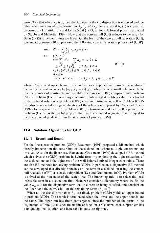
304 Chemical Engineering
term. Note that when jk is 1, then the jth term in the kth disjunction is enforced and theother terms are ignored. The constraints jkhjk
jk/jk are convex if hjkx is convex asdiscussed by Hiriart-Urruty and Lemaréchal (1993, p. 160). A formal proof is providedby Stubbs and Mehrotra (1999). Note that the convex hull (CH) reduces to the result byBalas (1985) if the constraints are linear. On the basis of the convex hull relaxation (CH),Lee and Grossmann (2000) proposed the following convex relaxation program of (GDP).
min ZL = ∑k∈K
∑j∈Jk
jkjk+fx
st gx≤ 0x = ∑
j∈Jkjk
∑j∈Jk
jk = 1 k ∈ K
0 ≤ jk ≤ jkxUjk j ∈ Jk k ∈ K
jkhjkjk/jk≤ 0 j ∈ Jk k ∈ K
A≤ a0 ≤ x jk ≤ xU 0 ≤ jk ≤ 1 j ∈ Jk k ∈ K
CRP
where xu is a valid upper bound for x and . For computational reasons, the nonlinearinequality is written as jkhjkjk/jk + ≤ 0 where is a small tolerance. Notethat the number of constraints and variables increases in (CRP) compared with problem(GDP). Problem (CRP) has a unique optimal solution and it yields a valid lower boundto the optimal solution of problem (GDP) (Lee and Grossmann, 2000). Problem (CRP)can also be regarded as a generalization of the relaxation proposed by Ceria and Soares(1999) for a special form of problem (GDP). Grossmann and Lee (2003) proved thatproblem (CRP) has the useful property that the lower bound is greater than or equal tothe lower bound predicted from the relaxation of problem (BM).
11.4 Solution Algorithms for GDP
11.4.1 Branch and Bound
For the linear case of problem (GDP), Beaumont (1991) proposed a BB method whichdirectly branches on the constraints of the disjunctions where no logic constraints areinvolved. Also for the linear case Raman and Grossmann (1994) developed a BB methodwhich solves the (GDP) problem in hybrid form, by exploiting the tight relaxation ofthe disjunctions and the tightness of the well-behaved mixed-integer constraints. Thereare also BB methods for solving problem (GDP). In particular, a disjunctive BB methodcan be developed that directly branches on the term in a disjunction using the convexhull relaxation (CRP) as a basic subproblem (Lee and Grossmann, 2000). Problem (CRP)is solved at the root node of the search tree. The branching rule is to select the leastinfeasible term in a disjunction first. Next, we consider a dichotomy where we fix thevalue jk = 1 for the disjunctive term that is closest to being satisfied, and consider onthe other hand the convex hull of the remaining terms (jk = 0).
When all the decision variables jk are fixed, problem (CRP) yields an upper boundto problem (GDP). The search is terminated when the lower and the upper bounds arethe same. The algorithm has finite convergence since the number of the terms in thedisjunction is finite. Also, since the nonlinear functions are convex, each subproblem hasa unique optimal solution, and hence the bounds are rigorous.

Advances in Logic-Based Optimization Approaches 305
11.4.2 Reformulation and Cutting Planes
Another approach for solving a linear GDP is to replace the disjunctions either bybig-M constraints or by the convex hull of each disjunction (Balas, 1985; Raman andGrossmann, 1994). For the nonlinear case, a similar way of solving the problem (GDP)is to reformulate it into the MINLP by restricting the variables jk in problem (CRP) to0–1 values. Alternatively, to avoid introducing a potentially large number of variablesand constraints, the GDP might also be reformulated as the MINLP problem (BM) byusing big-M parameters, although this leads to a weaker relaxation (Grossmann and Lee,2003). One can then apply standard MINLP solution algorithms (i.e. BB, OA, GBD,and ECP).To strengthen the lower bounds one can derive cutting planes using the convex hull
relaxation (CRP). To generate a cutting plane, the following 2-norm separation problem(SP), a convex QP, is solved:
min x= x−xBMnR Tx−xBMn
R s.t. gx≤ 0
x = ∑i∈Dk
ik k ∈ K
yikhikik/yik≤ 0 i ∈Dk k ∈ K∑i∈Dk
yik = 1 k ∈ K
Ay ≤ axik ∈ Rn 0 ≤ yik ≤ 1
SP
where xBMnR is the solution of problem (BM) with relaxed 0 ≤ yik ≤ 1. Problem (SP)
yields a solution point x∗ which belongs to the convex hull of the disjunction and isclosest to the relaxation solution xBMn
R . The most violated cutting plane is then given by
x∗ −xBMnR Tx−x∗≥ 0 (CP1)
The cutting plane in (CP1) is a valid inequality for problem (GDP). Problem (BM) ismodified by adding the cutting plane (CP1) as follows:
min Z = ∑k∈K
∑i∈Dk
ikyik+fx
s.t. gx≤ 0hikx≤Mik1−yik i ∈Dk k ∈ K∑i∈Dk
yik = 1 k ∈ K
Ay ≤ a Tx ≤ bx ∈ Rn 0 ≤ yik ≤ 1
CP
where Tx ≤ b is the cutting plane (CP1). Since we add a valid inequality to problem(BM), the lower bound obtained from problem (CP) is generally tighter than beforeadding the cutting plane.This procedure for generating the cutting plane can be used by solving the separation
problem (SP) only at the root node. It can also be used to strengthen the MINLP problem(BM) before applying methods such as OA, GBD, and ECP. It is also interesting to

306 Chemical Engineering
note that cutting planes can be derived in the xy space, especially when the objectivefunction has binary variables y.Another application of the cutting plane is to determine if the convex hull formulation
yields a good relaxation of a disjunction. If the value of x∗ − xBMnR is large, then it
is an indication that this is the case. A small difference between x∗ and xBMnR would
indicate that it might be better to simply use the big-M relaxation. It should also be notedthat Sawaya and Grossmann (2004) have recently developed the cutting plane methodfor linear GDP problems using the 1, 2, and norms, and relying on the theory ofsubgradient optimization.
11.4.3 GDP Decomposition Methods
Türkay and Grossmann (1996) have proposed logic-based OA and GBD algorithms forproblem (GDP) by decomposition into NLP and MILP subproblems. For fixed valuesof the Boolean variables, Yjk = true and Yik = false for j = i, the corresponding NLPsubproblem is derived from (GDP) as follows:
min Z =∑k∈K
ck+fx
s.t. gx≤ 0
hjkx≤ 0ck = jk
for Yjk = true j ∈ Jk k ∈ K (NLPD)
Bix = 0ck = 0
for Yik = false i ∈ Jk k ∈ K
x ∈ Rn c ∈ Rm
For every disjunction k only the constraints corresponding to the Boolean variable Yjkthat is true are enforced. Also, fixed charges jk are applied to these terms. After K
subproblems (NLPD) are solved, sets of linearizations l = 1 K are generated forsubsets of terms Ljk = lY l
jk = true, then one can define the following disjunctive OAmaster problem:
min Z =∑k∈K
ck+
s.t.≥ fxl+fxlTx−xlgxl+gxlTx−xl≤ 0
l= 1 L
Yjkhjkx
l+hjkxlTx−xl≤ 0 l ∈ Ljk
ck = jk
∨
¬YjkBkx = 0ck = 0
k ∈ K (MGDP)
Y= Truex ∈ Rn c ∈ Rm Y ∈ true falsem
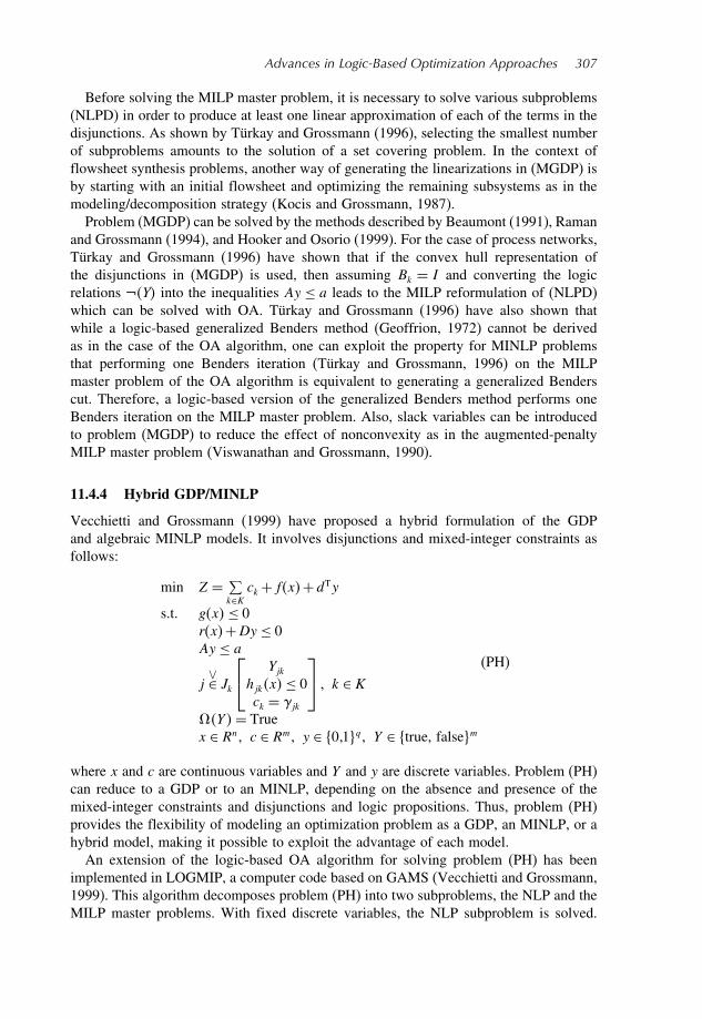
Advances in Logic-Based Optimization Approaches 307
Before solving the MILP master problem, it is necessary to solve various subproblems(NLPD) in order to produce at least one linear approximation of each of the terms in thedisjunctions. As shown by Türkay and Grossmann (1996), selecting the smallest numberof subproblems amounts to the solution of a set covering problem. In the context offlowsheet synthesis problems, another way of generating the linearizations in (MGDP) isby starting with an initial flowsheet and optimizing the remaining subsystems as in themodeling/decomposition strategy (Kocis and Grossmann, 1987).Problem (MGDP) can be solved by the methods described by Beaumont (1991), Raman
and Grossmann (1994), and Hooker and Osorio (1999). For the case of process networks,Türkay and Grossmann (1996) have shown that if the convex hull representation ofthe disjunctions in (MGDP) is used, then assuming Bk = I and converting the logicrelations ¬Y into the inequalities Ay ≤ a leads to the MILP reformulation of (NLPD)which can be solved with OA. Türkay and Grossmann (1996) have also shown thatwhile a logic-based generalized Benders method (Geoffrion, 1972) cannot be derivedas in the case of the OA algorithm, one can exploit the property for MINLP problemsthat performing one Benders iteration (Türkay and Grossmann, 1996) on the MILPmaster problem of the OA algorithm is equivalent to generating a generalized Benderscut. Therefore, a logic-based version of the generalized Benders method performs oneBenders iteration on the MILP master problem. Also, slack variables can be introducedto problem (MGDP) to reduce the effect of nonconvexity as in the augmented-penaltyMILP master problem (Viswanathan and Grossmann, 1990).
11.4.4 Hybrid GDP/MINLP
Vecchietti and Grossmann (1999) have proposed a hybrid formulation of the GDPand algebraic MINLP models. It involves disjunctions and mixed-integer constraints asfollows:
min Z = ∑k∈K
ck+fx+dTy
s.t. gx≤ 0rx+Dy ≤ 0Ay ≤ a
j
∨∈ Jk
Yjkhjkx≤ 0ck = jk
k ∈ K
Y = Truex ∈ Rn c ∈ Rm y ∈ 01q Y ∈ true, falsem
(PH)
where x and c are continuous variables and Y and y are discrete variables. Problem (PH)can reduce to a GDP or to an MINLP, depending on the absence and presence of themixed-integer constraints and disjunctions and logic propositions. Thus, problem (PH)provides the flexibility of modeling an optimization problem as a GDP, an MINLP, or ahybrid model, making it possible to exploit the advantage of each model.An extension of the logic-based OA algorithm for solving problem (PH) has been
implemented in LOGMIP, a computer code based on GAMS (Vecchietti and Grossmann,1999). This algorithm decomposes problem (PH) into two subproblems, the NLP and theMILP master problems. With fixed discrete variables, the NLP subproblem is solved.

308 Chemical Engineering
Then at the solution point of the NLP subproblem, the nonlinear constraints are linearizedand the disjunction is relaxed by convex hull to build a master MILP subproblem whichwill yield a new discrete choice of yY for the next iteration.
11.5 Global Optimization Algorithm of Nonconvex GDP
In the preceding sections of this chapter we assumed convexity in the nonlinear functions.However, in many applications nonlinearites give rise to nonconvex functions that mayyield local solutions, not guaranteeing the global optimality. Global optimization ofnonconvex programs has received increased attention due to their practical importance.Most of the deterministic global optimization algorithms are based on the spatial BBalgorithm (Horst and Tuy, 1996), which divides the feasible region of continuous variablesand compares lower bound and upper bound for fathoming each subregion. The one thatcontains the optimal solution is found by eliminating subregions that are proved not tocontain the optimal solution.For nonconvex NLP problems, Quesada and Grossmann (1995) proposed a spatial BB
algorithm for concave separable, linear fractional, and bilinear programs using linear andnonlinear underestimating functions (McCormick, 1976). For nonconvex MINLP, Ryooand Sahinidis (1995) and later Tawarmalani and Sahinidis (2002) developed BARON,which branches on the continuous and discrete variables with bounds reduction method.Adjiman et al. (1997, 2000) proposed the SMIN-BB and GMIN-BB algorithms fortwice-differentiable nonconvex MINLPs. Using a valid convex underestimation of generalfunctions as well as for special functions, Adjiman et al. (1996) developed the BBmethod which branches on both the continuous and discrete variables according tospecific options. The branch-and-contract method (Zamora and Grossmann, 1999) hasbilinear, linear fractional, and concave separable functions in the continuous variablesand binary variables, uses bound contraction, and applies the OA algorithm at eachnode of the tree. Kesavan and Barton (2000b) developed a generalized branch-and-cut(GBC) algorithm, and showed that their earlier decomposition algorithm (Kesavan andBarton, 2000a) is a specific instance of the GBC algorithm with a set of heuristics.Smith and Pantelides (1997) proposed a reformulation method combined with a spatialBB algorithm for nonconvex MINLP and NLP, which is implemented in the gPROMSmodeling system.
11.5.1 GDP Global Optimization Algorithms
We briefly describe two global optimization algorithms. The first was proposed by Leeand Grossmann (2001) and is for the case when the problem (GDP) involves bilinear,linear fractional, and concave separable functions. First, these nonconvex functions ofcontinuous variables are relaxed by replacing them with underestimating convex functions(McCormick, 1976; Quesada and Grossmann, 1995). Next, the convex hull of eachnonlinear disjunction is constructed to build a convex NLP problem (CRP). At the firststep, an upper bound is obtained by solving the nonconvex MINLP reformulation (BM)with the OA algorithm. This upper bound is then used for the bound contraction. Thefeasible region of continuous variables is contracted with an optimization subproblemthat incorporates the valid underestimators and the upper bound value and that minimizes

Advances in Logic-Based Optimization Approaches 309
or maximizes each variable in turn. The tightened convex GDP problem is then solvedin the first level of a two-level BB algorithm, in which a discrete BB search is performedon the disjunctions to predict lower bounds. In the second level, a spatial BB methodis used to solve nonconvex NLP problems for updating the upper bound. The algorithmexploits the convex hull relaxation for the discrete search and the fact that the spatial BBis restricted to fixed discrete variables in order to predict tight lower bounds.The second algorithm is by Bergamini et al. (2004); it does not require spatial BB
searches as it uses piecewise linear approximations. The algorithm considers the logic-based OA algorithm (Türkay and Grossmann, 1996) and is based on constructing a masterproblem that is a valid bounding representation of the original problem, and on solvingthe NLP subproblems to global optimality. The functions are assumed to be sums ofconvex, bilinear, and concave terms. To maintain rigorously the bounding properties ofthe MILP master problem, linear under- and overestimators for bilinear and concaveterms are constructed over a grid with the property of having zero gap in the finite setof points. The set of these approximation points is defined over subdomains defined bybounds of variables and solution points of the previous NLP subproblems. For bilinearterms, the convex envelope by McCormick is used. Disjunctions are used to formulatethe convex envelope in each subdomain, and the convex hull of these disjunctions isused to provide the tightest relaxation. It should be noted that binary variables are neededfor the discrete choice of the corresponding subdomains. Linear fractional functions aretreated similarly. Piecewise linear subestimations replace the concave terms.The solution of the NLP subproblems to global optimality can be performed by
fixing the topology variables in the MILP and by successively refining the grid of thepiecewise linear approximations. Alternatively, a general-purpose NLP algorithm forglobal optimization (e.g. BARON code by Tawarmalani and Sahinidis, 2002) can beused. It should be noted that the NLP subproblems are reduced problems, involving onlycontinuous variables related to a process with fixed structure. This allows the tighteningof the variable bounds, and therefore reduces the computational cost of solving it toglobal optimality.
11.6 Constraint Programming and Hybrid MILP/CP Methods
In order to overcome difficulties in modeling and scalability of MP models, a trend hasemerged to combine MP with symbolic logic reasoning into the quantitative. Amongthese attempts, one of the more promising approaches has been the development of CP,which has proved to be particularly effective in scheduling applications. CP is essentiallybased on the idea that inference methods can accelerate the search for a solution.CP (Hentenryck, 1989; Hooker, 2000) is a relatively new modeling and solution
paradigm that was originally developed to solve feasibility problems, but it has beenextended to solve optimization problems as well. CP is very expressive as continuousintegers as well as Boolean variables are permitted and moreover, variables can beindexed by other variables. Constraints can be expressed in algebraic form (e.g. hx≤ 0),as disjunctions (e.g. A1x≤ b1∨ A2x≤ b2), or as conditional logic statements (e.g. ifgx≤ 0 then rx≤ 0). In addition, the language can support special implicit functionssuch as the all different x1 x2 xn constraint for assigning different values to theinteger variables x1 x2 xn. The language consists of C++ procedures, although the

310 Chemical Engineering
recent trend has been to provide higher-level languages such as OPL. Other commercialCP software packages include ILOG Solver (ILOG, 1999), CHIP (Dincbas et al., 1988),and ECLiPSe (Wallace et al., 1997).Optimization problems in CP are solved as constraint satisfaction problems (CSP),
where we have a set of variables, a set of possible values for each variable (domain),and a set of constraints among the variables. The question to be answered is as follows:Is there an assignment of values to variables that satisfies all constraints? The solutionof CP models is based on performing constraint propagation at each node by reducingthe domains of the variables. If an empty domain is found the node is pruned. Branchingis performed whenever a domain of an integer, binary or Boolean variable has morethan one element, or when the bounds of the domain of a continuous variable do notlie within a tolerance. Whenever a solution is found, or a domain of a variable isreduced, new constraints are added. The search terminates when no further nodes mustbe examined. The effectiveness of CP depends on the propagation mechanism behindconstraints. Thus, even though many constructs and constraints are available, not all ofthem have efficient propagation mechanisms. For some problems, such as scheduling,propagation mechanisms have been proven to be very effective. Some of the mostcommon propagation rules for scheduling are the ‘time-table’ constraint (Le Pape, 1998),the ‘disjunctive-constraint’ propagation (Baptiste and Le Pape, 1996; Smith and Cheng,1993), the ‘edge-finding’ (Nuijten, 1994; Caseau and Laburthe, 1994), and the ‘not-first,not-last’ (Baptiste and Le Pape, 1996).Since MILP and CP approaches appear to have complementary strengths, in order
to solve difficult problems that are not effectively solved by either of the two, severalresearchers have proposed models that integrate the two paradigms. The integrationbetween MILP and CP can be achieved in two ways (Hooker, 2002; Hentenryck, 2002):
(1) By combining MILP and CP constraints into one hybrid model. In this case a hybridalgorithm that integrates constraint propagation with linear programming in a singlesearch tree is also needed for the solution of the model (e.g. Heipcke, 1999; Rodoseket al., 1999).
(2) By decomposing the original problem into two subproblems: one MILP and oneCP subproblem. Each model is solved separately and information obtained whilesolving one subproblem is used for the solution of the other subproblem (Jain andGrossmann, 2001; Bockmayr and Pisaruk, 2003).
Maravelias and Grossmann (2004) have recently developed a hybrid MILP/CP method forthe continuous time state-task-network (STN) model in which different objectives such asprofit maximization, cost minimization, and makespan minimization can be handled. Theproposed method relies on an MILP model that represents an aggregate of the originalMILP model. This method has been shown to produce order of magnitude reductions inCPU times compared to standalone MILP or CP models.
11.7 Examples in Process Integration
11.7.1 Synthesis of Separation System
This problem, a joint collaboration with BP (Lee et al., 2003), deals with the synthesisof a separation system of an ethylene plant in which the mixture to be separated includes

Advances in Logic-Based Optimization Approaches 311
A/BCDEFGH
ABCDEFGH
STATES TASKS
AB/CDEFGH
ABCD/CDEFGH
ABCDEF/CDEFGH
ABCDEF/EFGH
ABCD/EFGH
ABCDEF/GH
ABCDEFG/H
ABCDEFG
BCDEFGH
NON-SHARP
A/BCDEFG
AB/CDEFG
ABCD/CDEFG
ABCDEF/CDEFG
ABCDEF/EFG
ABCD/EFG
ABCDEF/G
B/CDEFGH
BCD/EFGH
BCD/CDEFGH
BCDEF/CDEFGH
BCDEF/EFGH
BCDEF/GH
BCDEFG/H
ABCDEF
BCDEFG
CDEFGH
A/BCDEF
AB/CDEF
ABCD/CDEF
ABCD/EF
BCDEF/G
B/CDEFG
BCD/CDEFG
BCDEF/CDEFG
BCDEF/EFG
BCD/EFG
CDEFG/H
CD/EFGH
CDEF/EFGH
CDEF/GH
BCDEF
CDEFG
ABCD
AB
BCD
EFG
CDEF
EFGH
GH
EF
CD
A
B
C
D
F
E
G
H
CD/EFG
CDEF/EFG
CDEF/G
B/CDEF
BCD/CDEF
BCD/EF
A/BCD
AB/CD
CD/EF
EF/GH
EFG/H
B/CD
EF/GG/H
E/F
C/D
A/B
H2
CH4
C2H4
C3H6
C2H6
C3H8
C4
C5
Figure 11.1 Superstructure of separation of ethylene plant
hydrogen, methane, ethane, ethylene, propane, propylene, and C4s, C5s, and C6s. Foreach potential separation task a number of separation technologies such as dephlegmators,membranes, PSA, physical and chemical absorption were considered in addition to thestandard distillation columns and cold boxes. The superstructure of this problem, whichincludes 53 separation tasks, is shown in Figure 11.1. This problem was formulated as aGDP problem and reformulated as an MINLP by applying both big-M and convex hulltransformations. The problem involved 5800 0–1 variables, 24 500 continuous variables,and 52 700 constraints, and was solved with GAMS DICOPT (CONOPT2/CPLEX) in3 h of CPU time on a Pentium III machine. Compared to the base-case design the optimalflowsheet that is shown in Figure 11.2 included a dephlegmator and a physical absorber,and one less distillation column, achieving a $20 million reduction in the cost, largelyfrom reduced refrigeration.
11.7.2 Retrofit Planning Problem
In this problem it is assumed that an existing process network is given where each processcan possibly be retrofitted for improvements such as higher yield, increased capacity,and reduced energy consumption. Given limited capital investments to make processimprovements and cost estimations over a given time horizon, the problem consistsof identifying those modifications that yield the highest economic improvement in termsof economic potential, which is defined as the income from product sales minus the costof raw materials, energy, and process modifications. Sawaya and Grossmann (2004) havedeveloped a GDP model for this problem, which is a modification of work by Jacksonand Grossmann (2002).

312 Chemical Engineering
ABCDEFGH
AB
CDEFGH
EF
CD
B
A
D
C
E
F
H
G
A/B
CH4
C2H4
C3H6
C2H6
C3H8
C4
C5
H2
EFGH
Cold box
Deethanizer
Dephlegmator
100F480Psig
480Psig
480Psig
84F190Psig
169F160Psig
83F160Psig
– 41F
160Psig
– 141F900Psig
– 51F140Psig
900Psig
–31F140Psig
DE
FG
GF
EF
C
D
GH
Depropanizer
C3Splitter
226F160Psig
Compressor
Heater
Cooler
Valve
74F170Psig
214F170Psig
109F140Psig
Debutanizer
236F140Psig
123F140Psig
99F140Psig
72F140Psig
238F140Psig
AB
CD
Chemicalabsorber
410 Mkwh/yr
Valve
Compressor
Pump
Pump
Figure 11.2 Optimal structure of ethylene plant
For a 10-process instance (Figure 11.3) that involves the production of products(G,H,I,J,K,L,M) from raw materials (A,B,C,D,E), the 4-period MILP model was for-mulated with the big-M and convex hull reformulations. The former involved 320 0–1variables, 377 continuous variables, and 1957 constraints; the latter involved 320 0–1 vari-ables, 1097 continuous variables, and 2505 constraints. The big-M model was solved in1913 s and 1 607 486 nodes, while the latter required only 5.8 s and 2155 nodes. Thisreduction was achieved because the convex hull formulation had a gap of only 7.6%versus the 60.3% gap of the big-M model. It should be noted that with 120 cuts the gapin the big-M model reduced to only 7.9%, with which the MILP was solved in a total of68 s, of which 22 were for the cut generation.
11.7.3 Wastewater Treatment Network
This example corresponds to a synthesis problem of a distributed wastewater multi-component network, which is taken from Galan and Grossmann (1998). Given a set ofprocess liquid streams with known composition, a set of technologies for the removal ofpollutants, and a set of mixers and splitters, the objective is to find the interconnectionsof the technologies and their flowrates to meet the specified discharge composition ofpollutant at minimum total cost. Discrete choices involve deciding what equipment to usefor each treatment unit. Figure 11.4 shows the superstructure of a specific example withthree contaminants and three choices of separation technologies per contaminant. Leeand Grossmann (2001) formulated the problem as a GDP model that involves 9 Boolean
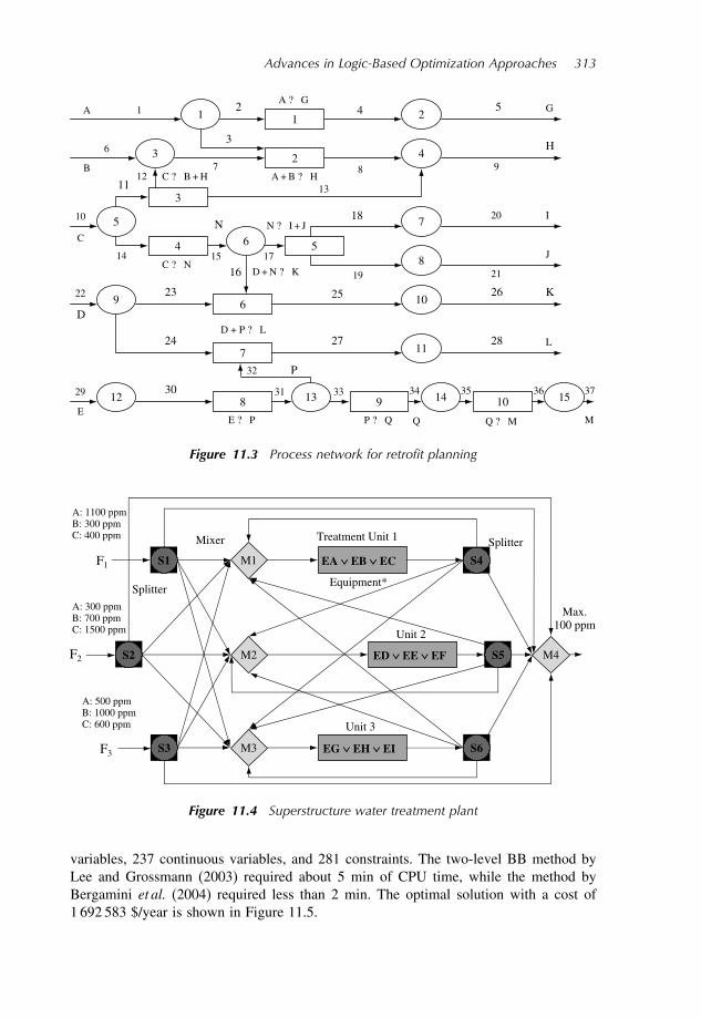
Advances in Logic-Based Optimization Approaches 313
3
4
10
5
7
6
98 13
2
3 4
5 7
8
9 10
11
12 14 15
1
D
H
K
P
N
2
3
4 5
11 13
16
18
23
24
25 26
27 28
30
6
1
2
37363534 33
32
3129
22
6
21
20
19
1715
10
14
129 87
1
Q M
L
J
I
G
E
C
B
A
E ? P
C ? N
D + P ? L
D + N ? K
P ? Q Q ? M
A + B ? H
A ? G
C ? B + H
N ? I + J
Figure 11.3 Process network for retrofit planning
S1
M3
M2
S6
S5
S4M1
S3
S2 M4
Treatment Unit 1
Unit 3
Unit 2
EA ∨ EB ∨ EC
ED ∨ EE ∨ EF
EG ∨ EH ∨ EI
F1
F2
F3
Equipment*Splitter
Mixer Splitter
Max.100 ppm
A: 1100 ppmB: 300 ppmC: 400 ppm
A: 300 ppmB: 700 ppmC: 1500 ppm
A: 500 ppmB: 1000 ppmC: 600 ppm
Figure 11.4 Superstructure water treatment plant
variables, 237 continuous variables, and 281 constraints. The two-level BB method byLee and Grossmann (2003) required about 5 min of CPU time, while the method byBergamini et al. (2004) required less than 2 min. The optimal solution with a cost of1 692 583 $/year is shown in Figure 11.5.

314 Chemical Engineering
C: 40%
S1
M3
M2
S6
S5
S4M1
S3
S2 M4
EI
EF
F1
F2
F3
20 ton/h
15 ton/h
5 ton/h
7.25612.744
15
5
40
27.256
37.603
40 ton/h2.397
24.859
37.603
24.859
37.603
40
A: 90%, C: 40%
A: 50%, B: 99%, C: 80% A: 100 ppmB: 100 ppmC: 100 ppm
M3
M2
M1
M4
EA
Figure 11.5 Optimal wastewater treatment plant
11.8 Examples in Supply Chain Management
11.8.1 Hydrocarbon Field Infrastructure Planning
In this example we consider the design, planning, and scheduling of an offshore oilfieldinfrastructure over a planning horizon of 6 years divided into 24 quarterly periods wheredecisions need to be made (Van den Heever and Grossmann, 2000). The infrastructureunder consideration consists of 1 production platform (PP), 2 well platforms (WP), and25 wells and connecting pipelines (Figure 11.6). Each oilfield (F) consists of a number
Productionplatform
Wellplatform
Wellplatform
Sales
Fields
Reservoirs
Wells
Figure 11.6 Configuration of fields, well platforms, and production platforms

Advances in Logic-Based Optimization Approaches 315
of reservoirs (R), while each reservoir in turn contains a number of potential locationsfor wells (W) to be drilled. Design decisions involve the capacities of the PPs and WPs,as well as decisions regarding which WPs to install over the whole operating horizon.Planning decisions involve the production profiles in each period, as well as decisionsregarding when to install PPs and WPs included in the design, while scheduling decisionsinvolve the selection and timing of drilling of the wells. This leads to an MINLP modelwith 9744 constraints, 5953 continuous variables, and 700 0–1 variables. An attempt tosolve this model with a commercial package such as GAMS (Brooke et al., 1998) (usingDICOPT (Viswanathan and Grossmann, 1990)) with CPLEX 6.6 (ILOG, 2001) for theMILPs and CONOPT2 (Drud, 1992) for the NLPs on an HP 9000/C110 workstationresults in a solution time of 19 386 CPU seconds.To overcome this long solution time, Van den Heever and Grossmann (2000) devel-
oped an iterative aggregation/disaggregation algorithm which solved the model in 1423CPU seconds. This algorithm combines the concepts of bilevel decomposition, timeaggregation, and logic-based methods. The application of this method led to an orderof magnitude reduction in solution time, and produced an optimal net present value of$68 million. Figure 11.7 shows the total oil production over the 6-year horizon, whileTable 11.1 shows the optimal investment plan obtained. Note that only 9 of the 25 wellswere chosen in the end. This solution resulted in savings in the order of millions of dollarscompared to the heuristic method used in the oilfield industry that specifies almost allthe wells being drilled.
11.8.2 Supply Chain Problem
The example problem in Figure 11.8, a multisite continuous production facility formultiple products, was solved by Bok et al. (2000) over a 7-day horizon to illustrate theperformance of their model in three cases: (1) no intermittent deliveries of raw materialswithout product changeovers; (2) intermittent deliveries without changeovers; and(3) intermittent deliveries with changeovers. It is obvious that case 3 is the most rigorousand detailed. Cases 1 and 2 can be obtained by relaxing the discrete nature of case 3.In the case of intermittent deliveries, the minimum time interval between successive
0
20
40
60
80
1999Jan.
1999Jul.
2000Jan.
2001Jan.
2001Jul.
2002Jan.
2003Jan.
2004Jan.
2002Jul.
2003Jul.
2004Jul.
2000Jul.
Prod
uctio
n (1
000
barr
els/
day)
Figure 11.7 Production profile over 6-year horizon

316 Chemical Engineering
Table 11.1 The optimal investment plan
Item Period invested
PP Jan 1999WP1 Jan 1999
Reservoir Well2 4 Jan 19993 1 Jan 19995 3 Jan 19994 2 Apr 19997 1 Jul 19996 2 Oct 19991 2 Jan 20009 2 Jan 2000
10 1 Jan 2000
C3
C5
C4
P1. K1
P2. K1
P4. K2
P4. K1
C1
C6 C2
C4
C5 P4. K2
P4. K1
L1
L1
L4
L3
Site 1
Site 2
P2. K2
P3. K1
P3. K2
P3. K3
P3. K4
P2. K1
P2. K2
P3. K1
P3. K2
P3. K3
Figure 11.8 Multisite production facility for supply chain problem
deliveries is assumed to be 2 days regardless of the chemicals or the sites. The problemwas modeled using the GAMS modeling language and solved in the full space using theCPLEX solver on an HP 9000/7000. The optimization results for this example are asfollows. In case 1, 2034 variables and 1665 constraints are required and no 0–1 variable

Advances in Logic-Based Optimization Approaches 317
is needed because there are no intermittent deliveries nor any changeovers. The problemwas solved in only 2 s CPU time. The more rigorous the model (cases 2 or 3), thelarger the number of 0–1 variables required. This in turn results in more computationtime for the optimization. Case 2 for changeovers required 224 0–1 variables, 1810continuous variables, and 1665 constraints solving in 4min CPU. Case 3, which includeschangeovers and intermittent supplies, involved 392 0–1 variables, 1642 continuousvariables, and 1665 constraints solving in 8 min CPU. Figure 11.9 shows the optimizationresults for case 3 that considers the intermittent deliveries and changeovers. Bok et al.(2000) proposed a decomposition algorithm in order to be able to solve larger problems.
11.8.3 Scheduling of Batch Plants
Consider the batch scheduling problem that is given through the STN shown inFigure 11.10, which is an extension of the work by Papageorgiou and Pantelides (1996).
0
50
100
150
200
250
300
1 3 5 7
Mill
ion
LB
Time horizon (day)
( j3,l1,c1)
( j3,l2,c2)
( j3,l1,c2)
( j3,l2,c1)
Sales amount for chemical 3
0
1
2
3
4
5
6
7
Mill
ion
LB
Shortfall for chemical 3
( j3,l1,c1)
( j3,l2,c1)
( j3,l1,c2)
( j3,l2,c2)
1 3 5 6 7Time horizon (day)
2 4
0
20
40
60
80
100
120
140
1 3 5 6 7Time horizon (day)
Mill
ion
LB
Inventory for products
2 4
( j3,c1)
( j3,c2)
( j4,c1)
( j4,c2)
2 4 6
Figure 11.9 Results for sales, inventory, and shortfalls in supply chain problem

318 Chemical Engineering
T10 T11 T21 T22 T23F2 S10 INT1 S21 S22 P1
T61 T62 T70 T71 T72F5 S61 INT4 S70 S71 P4
T20F1
T60F6
S20
S72
T31 T32F4 S31
T30F3 S30
T40 T41INT2S40
T50 T51S50
INT3
P2
P3
S60
0.25
0.75
0.80
0.20 0.50
0.50
0.40
0.60
0.65
0.35
0.95
0.05
0.15
0.85
Figure 11.10 State-task-network example
The STN consists of 27 states, 19 tasks, and has 8 equipment units available for theprocessing. The objective is to find a schedule that produces 5 tons each for products P1,P2, P3, and P4. The problem was originally modeled with the continuous-time MILP byMaravelias and Grossmann (2003) involving around 400 0–1 variables, 4000 continuousvariables, and 6000 constraints. Not even a feasible solution to this problem could befound with CPLEX 7.5 after 10 h. In contrast, the hybrid MILP/CP model requiredonly 2 s and five major iterations between the MILP and CP subproblems! Note that theoptimal schedule shown in Figure 11.11 is guaranteed to be the global optimum solution.
T10 (3) T21 (5)
T31 (5)
T32 (3) T32 (3) T32 (3)
T31 (7)
T30(3) T60 (1)
T20(1)
T61 (3)
T23 (5)
t (hr)
T50 (5) T40 (5)
T70 (6)
T11 (3) T22 (5) T41(5)
T71(6) T72(6)
U1
U2
U3
U4
U5
U6
U7
U8
0 2 4 6 8 10 12 14 15
Figure 11.11 Optimal schedule

Advances in Logic-Based Optimization Approaches 319
11.9 Conclusions
Mixed-integer optimization techniques (MILP, MINLP) have proved to be essential inmodeling process integration problems (process synthesis and design) as well as supplychain management problems (planning and scheduling). The former tends to be largelynonlinear, while the latter tends to be linear. Major barriers that have been encounteredwith these techniques are modeling, scaling, and nonconvexities. It is the first two issuesthat have motivated logic-based optimization as a way of facilitating the modeling ofdiscrete/continuous problems, and of reducing the combinatorial search space. The GDPformulation has shown to be effective in terms of providing a qualitative/quantitativeframework for modeling, and an approach that yields tighter relaxations through theconvex hull formulation. It was also shown that global optimization algorithms can bedeveloped for GDP models and solved in reasonable time for modest-sized problem.Finally, the recent emergence of CP offers an alternative approach for handling logic indiscrete scheduling problems. Here the development of hybrid methods for schedulingseems to be particularly promising for achieving order of magnitude reductions in thecomputations. The power and scope of the techniques were demonstrated on a variety ofprocess integration and supply chain management problems.
Acknowledgments
The author gratefully acknowledges financial support from the National Science Foun-dation under Grant ACI-0121497 and from the industrial members of the Center forAdvanced Process Decision-Making (CAPD) at Carnegie Mellon University.
References
Adjiman C.S., Androulakis I.P., Maranas C.D. and Floudas C.A. 1996. A global optimizationmethod, BB, for process design, Comput. Chem. Eng., 20(Suppl.), S419–S424.
Adjiman C.S., Androulakis I.P. and Floudas C.A. 1997. Global optimization of MINLP problemsin process synthesis and design, Comput. Chem. Eng., 21(Suppl.), S445–S450.
Adjiman C.S., Androulakis I.P. and Floudas C.A. 2000. Global optimization of mixed-integernonlinear problems, AIChE J., 46(9), 1769–1797.
Balas E. 1965. An additive algorithm for solving linear programs with zero-one variables, Oper.Res., 13, 517–546.
Balas E. 1979. Disjunctive programming, Ann. Discrete Math., 5, 3–51.Balas E. 1985. Disjunctive programming and a hierarchy of relaxations for discrete optimization
problems, SIAM J. Alg. Discrete Methods, 6, 466–486.Balas E., Ceria S. and Cornuejols G. 1993. A lift-and-project cutting plane algorithm for mixed
0-1 programs, Math. Program., 58, 295–324.Baptiste P. and Le Pape C. 1996. Disjunctive constraints for manufacturing scheduling: Principles
and extensions, Int. J. Comput. Integr. Manufacturing, 9(4), 306–341.Beaumont N. 1991. An algorithm for disjunctive programs, Eur. J. Oper. Res., 48, 362–371.Benders J.F. 1962. Partitioning procedures for solving mixed variables programming problems,
Numerische Mathematik, 4, 238–252.

320 Chemical Engineering
Bergamini M.L., Aguirre P. and Grossmann I.E. 2004. Logic Based Outer Approximation forGlobal Optimization of Synthesis of Process Networks, submitted for publication.
Bisschop J. and Entriken R. 1993. AIMMS: The Modeling System. Paragon Decision Technology.Bockmayr A. and Pisaruk N. 2003. Detecting infeasibility and generating cuts for MIP using CP.
In, Proceedings of CP-AI-OR 2003, 24–34.Bok J.-K., Grossmann I.E. and Park S. 2000. Supply chain optimization in continuous flexible
process networks, I&EC Res., 39, 1279–1290.Borchers B. and Mitchell J.E. 1994. An improved branch and bound algorithm for mixed integer
nonlinear programming, Comput. Oper. Res., 21, 359–367.Brooke A., Kendrick D., Meeraus A. and Raman R. 1998. GAMS Language Guide. GAMS
Development Corporation, Washington, DC.Caseau Y. and Laburthe F. 1994. Improved CLP scheduling with task intervals. In, Proceedings of
11th International Conference on Logic Programming.Ceria S. and Soares J. 1999. Convex programming for disjunctive optimization, Math. Program.,
86(3), 595–614.Crowder H.P., Johnson E.L. and Padberg M.W. 1983. Solving large-scale zero-one linear program-
ming problems, Oper. Res., 31, 803–834.Dakin R.J. 1965. A tree search algorithm for mixed integer programming problems, Comput. J., 8,
250–255.Dincbas M., Van Hentenryck P., Simonis H., Aggoun A., Graf T. and Berthier F. 1988. The con-
straint logic programming language CHIP. In, FGCS-88: Proceedings of International Conferenceon Fifth Generation Computer Systems, Tokyo, pp. 693–702.
Duran M.A. and Grossmann I.E. 1986. An outer-approximation algorithm for a class of mixed-integer nonlinear programs, Math. Program., 36, 307–339.
Drud A.S. 1992. CONOPT – A Large-Scale GRG Code, ORSA J. Comput., 6, 207–216.Fletcher R. and Leyffer S. 1994. Solving mixed nonlinear programs by outer approximation, Math.
Program., 66(3), 327–349.Fourer R., Gay D.M. and Kernighan B.W. 1992. AMPL: A Modeling Language for Mathematical
Programming. Duxbury Press, Belmont, CA.Galan B. and Grossmann I.E. 1998. Optimal design of distributed wastewater treatment networks,
Ind. Eng. Chem. Res., 37, 4036–4048.Geoffrion A.M. 1972. Generalized Benders decomposition, J. Optimization Theory Appl., 10(4),
237–260.Gomory R.E. 1958. Outline of an algorithm for integer solutions to linear programs, Bull. Am.
Math. Soc., 64, 275–278.Grossmann I.E. 2002. Review of nonlinear mixed-integer and disjunctive programming techniques
for process systems engineering, J. Optimization Eng., 3, 227–252.Grossmann I.E. and Lee S. 2003. Generalized disjunctive programming: nonlinear convex hull
relaxation and algorithms, Comput. Optimization Appl., 26, 83–100.Grossmann I.E., Caballero J.P. and Yeomans H. 1999. Mathematical programming approaches to
the synthesis of chemical process systems, Korean J. Chem. Eng., 16(4), 407–426.Grossmann I.E., van den Heever S.A. and Harjunkoski I. 2002. Discrete optimization methods and
their role in the integration of planning and scheduling, AIChE Symposium Series No. 326, Vol.98, pp. 150–168.
Gupta O.K. and Ravindran V. 1985. Branch and bound experiments in convex nonlinear integerprogramming, Manag. Sci., 31(12), 1533–1546.
Heipcke S. 1999. An example of integrating constraint programming and mathematical program-ming, Electron. Notes Discrete Math., 1(1).
Hentenryck P.V. 1989. Constraint Satisfaction in Logic Programming. MIT Press, Cambridge, MA.Hentenryck P.V. 2002. Constraint and integer programming in OPL, INFORMS J. Comput., 14(4),
345–372.

Advances in Logic-Based Optimization Approaches 321
Hiriart-Urruty J. and Lemaréchal C. 1993. Convex Analysis and Minimization Algorithms.Springer-Verlag, Berlin.
Hooker J. 2000. Logic Based Methods for Optimization: Combining Optimization and ConstraintSatisfaction. John Wiley and Sons Inc., New York.
Hooker J.N. 2002. Logic, optimization, and constraint programming, INFORMS J. Comput., 4(4),295–321.
Hooker J.N. and Osorio M.A. 1999. Mixed logical/linear programming, Discrete Appl. Math.,96–97(1–3), 395–442.
Horst R. and Tuy H. 1996. Global Optimization: Deterministic Approaches, 3rd edition. Springer-Verlag, Berlin.
ILOG. 1999. ILOG OPL Studio 2.1., User’s Manual. ILOG.Jackson J.R. and Grossmann I.E. 2002. High level optimization model for the retrofit planning of
process networks, I&EC Res., 41, 3762–3770.Jain V. and Grossmann I.E. 2001. Algorithms for hybrid MILP/CP model for a class of optimization
problems, INFORMS J. Comput., 13, 258–276.Johnson E.L., Nemhauser G.L. and Savelsbergh M.W.P. 2000. Progress in linear programming
based branch-and-bound algorithms: an exposition, INFORMS J. Comput., 12, 2–23.Kallrath J. 2000. Mixed integer optimization in the chemical process industry: experience, potential
and future, Trans. I. Chem. E, 78(Part A), 809–822.Kesavan P. and Barton P.I. 2000a. Decomposition algorithms for nonconvex mixed-integer non-
linear programs, Am. Inst. Chem. Eng. Symp. Ser., 96(323), 458–461.Kesavan P. and Barton P.I. 2000b. Generalized branch-and-cut framework for mixed-integer non-
linear optimization problems, Comput. Chem. Eng., 24, 1361–1366.Kelley J.E. Jr. 1960. The cutting-plane method for solving convex programs, J. SIAM, 8, 703.Kocis G.R. and Grossmann I.E. 1987. Relaxation strategy for the structural optimization of process
flowsheets, Ind. Eng. Chem. Res., 26, 1869.Land A.H. and Doig A.G. 1960. An automatic method for solving discrete programming problems,
Econometrica, 28, 497–520.Lee S. and Grossmann I.E. 2000. New algorithms for nonlinear generalized disjunctive program-
ming, Comput. Chem. Eng., 24, 2125–2141.Lee S. and Grossmann I.E. 2001. A global optimization algorithm for nonconvex generalized dis-
junctive programming and applications to process systems, Comput. Chem. Eng., 25, 1675–1697.Lee S. and Grossmann I.E. 2003. Global optimization of nonlinear generalized disjunctive pro-
gramming with bilinear equality constraints: Applications to process networks, Comput. Chem.Eng., 27, 1557–1575.
Lee S., Logsdon J.S., Foral M.J. and Grossmann I.E. 2003. Superstructure optimization of theolefin separation process. In, Proceedings ESCAPE-13, Kraslawski A. and Turunen I. (Eds.),pp. 191–196.
Le Pape C. 1998. Implementation of resource constraints in ILOG SCHEDULE: A library for thedevelopment of constrained-based scheduling systems, Intell. Syst. Eng., 3(2), 55–66.
Leyffer S. 2001. Integrating SQP and branch-and-bound for mixed integer nonlinear programming,Comput. Optimization Appl., 18, 295–309.
Lovász L. and Schrijver A. 1991. Cones of matrices and set-functions and 0-1 optimization, SIAMJ. Optimization, 12, 166–190.
Maravelias C.T. and Grossmann I.E. 2003. A new general continuous-time state task networkformulation for short term, scheduling of multipurpose batch plants, I&EC Res., 42, 3056–3074.
Maravelias C.T. and Grossmann I.E. 2004. A hybrid MILP/CP decomposition approach for thecontinuous time scheduling of multipurpose batch plants, Comput. Chem. Eng. (in press).
McCormick G.P. 1976. Computability of global solutions to factorable nonconvex programs: partI – convex underestimating problems, Math. Program., 10, 147–175.
Nemhauser G.L. and Wolsey L.A. 1988. Integer and Combinatorial Optimization. Wiley-Interscience, New York.

322 Chemical Engineering
Nuijten W.P.M. 1994. Time and resource constrained scheduling: A constraint satisfactionapproach. Ph.D. Thesis, Eindhoven University of Technology.
ILOG 2001. ILOG OPL Studio 3.5: The optimization Language, ILOG Inc.Papageorgiou L.G. and Pantelides C.C. 1996. Optimal campaign planning/scheduling of multipur-
pose batch/semicontinuous plants. 2. Mathematical decomposition approach, Ind. Eng. Chem.Res., 35, 510–529.
Quesada I. and Grossmann I.E. 1992. An LP/NLP based branch and bound algorithm for convexMINLP optimization problems, Comput. Chem. Engng., 16(10/11), 937–947.
Quesada I. and Grossmann I.E. 1995. A global optimization algorithm for linear fractional andbilinear programs, J. Global Optimization, 6(1), 39–76.
Raman R. and Grossmann I.E. 1991. Relation between MILP modelling and logical inference forchemical process synthesis, Comput. Chem. Eng., 15(2), 73–84.
Raman R. and Grossmann I.E. 1994. Modelling and computational techniques for logic basedinteger programming, Comput. Chem. Eng., 18(7), 563–578.
Rodosek R., Wallace M.G. and Hajian M.T. 1999. A new approach to integrating mixed integerprogramming and constraint logic programming, Ann. Oper. Res., 86, 63–87.
Ryoo H.S. and Sahinidis N.V. 1995. Global optimization of nonconvex NLPs and MINLPs withapplications in process design, Comput. Chem. Eng., 19(5), 551–566.
Sawaya N.W. and Grossmann I.E. 2004. A cutting plane method for solving linear-generalizeddisjunctive programming problems (submitted).
Sherali H.D. and Adams W.P. 1990. A hierarchy of relaxations between the continuous and convexhull representations for zero-one programming problems, SIAM J. Discrete Math., 3(3), 411–430.
Smith E.M.B. and Pantelides C.C. 1997. Global optimization of nonconvex NLPs and MINLPswith applications in process design, Comput. Chem. Eng., 21(1001), S791–S796.
Smith S.F. and Cheng C-C. 1993. Slack-based heuristics for constrained satisfaction scheduling.Proceedings of 11th National Conference on Artificial Intelligence.
Stubbs R. and Mehrotra S. 1999. A branch-and-cut method for 0-1 mixed convex programming,Mathematical Programming, 86(3), 515–532.
Tawarmalani M. and Sahinidis N.V. 2002. Convexification and global optimization in continuousand mixed-integer nonlinear programming: Theory, algorithms, software, and applications. In,Nonconvex Optimization and Its Applications Series, Vol. 65. Kluwer Academic Publishers,Dordrecht.
Türkay M. and Grossmann I.E. 1996. Logic-based MINLP algorithms for the optimal synthesis ofprocess networks, Comput. Chem. Eng., 20(8), 959–978.
Van den Heever S.A. and Grossmann I.E. 2000. An iterative aggregation/disaggregation approachfor the solution of a mixed integer nonlinear oilfield infrastructure planning model, I&EC Res.,39, 1955–1971.
Van Roy T.J. and Wolsey L.A. 1986. Valid inequalities for mixed 0-1 programs, Discrete Appl.Math., 14, 199–213.
Vecchietti A. and Grossmann I.E. 1999. LOGMIP: a disjunctive 0-1 nonlinear optimizer for processsystems models, Comput. Chem. Eng., 23, 555–565.
Viswanathan J. and Grossmann I.E. 1990. A combined penalty function and outer-approximationmethod for MINLP optimization, Comput. Chem. Eng., 14, 769.
Wallace M., Novello S. and Schimpf J. 1997. ECLiPSe: a platform for constraint logic program-ming, ICL Syst. J., 12(1), 159–200.
Westerlund T. and Pettersson F. 1995. An extended cutting plane method for solving convexMINLP problems, Comput. Chem. Eng., 19(Suppl.), S131–S136.
Williams H.P. 1985. Mathematical Building in Mathematical Programming. JohnWiley, Chichester.Yuan X., Zhang S., Piboleau L. and Domenech S. 1988. Une Methode d’optimization Nonlineare
en Variables Mixtes pour la Conception de Porcedes, Rairo Recherche Operationnele, 22, 331.Zamora J.M. and Grossmann I.E. 1999. A branch and bound algorithm for problems with concave
univariate, bilinear and linear fractional terms, J. Global Optim., 14(3), 217–249.

12Integration of Process Systems
Engineering and Business DecisionMaking Tools: Financial Risk
Management and Other EmergingProcedures
Miguel J. Bagajewicz
12.1 Introduction
Economics has always been part of engineering, so talking about its integration in ourdiscipline seems rather odd. Moreover, many companies, especially those dealing withrisky projects, employ advanced financial tools in their decision making. For example,the oil industry is relatively more sophisticated than other industries in its supply chainmanagement tools and the associated finances. However, these are not widespread toolsthat all engineers employ and certainly not tools that are used in education or in academicpapers. Indeed, only certain aspects of the tools that economists and financiers use, namelya few profitability measures, are fully integrated into our education and engineeringacademic circles. This has started to change in recent years, but many tools are stillcompletely out of sight for mainstream chemical engineers.This is not a review article, so not all the work that has been published on the matter
will be cited or discussed. Rather, the intention is to discuss some of the more relevantand pressing issues and provide some direction for future work. It is also an article thattargets engineers as the audience.
Chemical Engineering: Trends and Developments. Edited by Miguel A. Galán and Eva Martin del ValleCopyright 2005 John Wiley & Sons, Inc., ISBN 0-470-02498-4 (HB)

324 Chemical Engineering
As a motivating example, one could start with the following statement of a typicalprocess design problem.
‘Design a plant to produce chemical X, with capacity Y’
For a long time, this is the problem that many capstone design classes used to propose tostudents to solve (and some still do). This is fairly well known. The answer is a flowsheet,optimized to follow certain economics criteria, with a given cash flow profile (costsand prices are given and are often considered fixed throughout time), from which a netpresent value and a rate of return is obtained. In the 1980s, environmental considerationsstarted to be added, but these were mostly used as constraints that in the end usuallyincreased costs. It is only recently that engineers started to talk about green engineeringand sustainability, but in most cases, these are still considered as constraints of the abovedesign problem, not as valid objectives.Reality is, however, more complex than the assumptions used for the above problem:
raw materials change quality and availability, demands may be lower than expected,and products may require different specifications through time, all of which should beaccomplished with one plant. So in the 1980s engineers proposed to solve the followingflexible design problem.
‘Design a flexible plant to produce chemical X, with capacity Y, capable of working in thegiven ranges of raw materials availability and quality and product specifications’
While the problem was a challenge to the community, it hardly incorporated any neweconomic considerations. The next step was to include uncertainty. Thus the revisedversion was:
‘Design a plant to produce chemical X, taking into account uncertain raw materials andproduct prices, process parameters, raw material availability and product demand, given theforecasts, and determine when the plant should be built as well as what expansions areneeded’
Substitute ‘plant’ with ‘network of processes’ or ‘product’ and you have supply chainproblems or product engineering.
This has been the typical problem of the 1990s. However, very few industries haveembraced the tools and the procedures and only a few schools teach it at the undergraduatelevel. As noted, this was later extended to networks of plants and supply chains, a subjectthat is still somewhat foreign in undergraduate chemical engineering education. Noticefirst that the fixed capacity requirement and the flexibility ranges are no longer included.The engineer is expected to determine the right capacity and the level of flexibility thatis appropriate for the design. In doing so, this maximizes expectation of profit. The profitmeasures (net present value or rate of return), however, did not change and are the sameas the one engineers have been using for years. The novelty is the planning aspect andthe incorporation of uncertainty.In addition, one has to realize that not all design projects are alike. Some are constrained
by spending and some not, some are performed to comply with regulations and do notnecessarily target profit, but rather cost. Thus, the type of economic analysis and theassociated tools change.Where do the engineers go from here? This chapter addresses some answers to this
question. Many of the most obvious pending questions/issues, some of which intersectwith others being already explored, are as follows:

Integration of PSE and Business Tools 325
• What is the financial risk involved in a project?• What is the project impact on of the financial status of the company that is consideringthis project, namely indicators such as,
– liquidity ratios (assets to liabilities)?– cash position, debts, etc?– short-, medium-, and long-term shareholder value, or in the case of a privatecompany the dividends, among others?
• How does the size of the company in relation to the capital involved in the projectshape the decision maker’s attitudes? It is not the same type of decision makingone makes when belonging to a big corporation rather than to a medium-size privatecompany, even when the financial indicators are similar. In other words, the questionat large is how the project impacts on company market value.
• How the decision making related to the project can reflect the strategic plans of thecompany and, most importantly, vice versa, that is, how to take into account thestrategic plan of the company at the level of project or investment decision making?
• Can ‘here and now’ decisions and design parameters be managed in relation to targetsor aspiration levels for the different indicators listed above?
• Can short- and long-term contracts and options be factored in at the time of thedecision making, not afterwards as control actions, to increase profitability?
• When should projects be based on taking equity and be undertaken with no incrementin profit because they are instrumental for other projects?
• Can one plan to alter the exogenous parameters, like prices, demands, to affect theexpected profit and/or the aforementioned indicators?
• Should one consider advertisement as part of the decision making, or product presen-tation (form, color, etc.), that is, the psychology of the user?
• Should sociology/psychology/advertisement/etc. be incorporated into the decisionmaking by modeling the different decisions vis-à-vis the possible response of the mar-ket? In other words, should one start considering the market demand as susceptible tobeing shaped, rather than using it as simple forecasted data?
The answer to the above list of questions (which is by no means exhaustive) is slowlyand strongly emerging. The latest Eighth International Symposium on Process SystemsEngineering held in China (PSE 2003) had many of the above issues as the central theme,but there is substantial earlier pioneering work. For example, in an article mostly devotedto prepare us for the information technology (IT) age (now in full development), and itsimpact on corporate management, Robertson et al. (1995) examined the lack of propercommunication in the corporate flow loop (Figure 12.1). They argue that the four majorcomponents of this loop (manufacturing, procuring, managing, and marketing) operatealmost as separate entities with minimal data sharing.Notwithstanding the lack of data sharing, which will (or is being) corrected, the real
issue is that the different elements of the loop also start to share the same goals andmethods, as Bunch and Iles (1998) argued. In many of the examples illustrated later inthis chapter, decisions at the level of manufacturing, like for example the schedulingof operations, are influenced by the company’s cash position and are related to pric-ing, etc. This involves marketing, procuring, and manufacturing in the solution of theproblem. Corporate management, procuring, and marketing should also work togetherto solve investment problems, etc. This is the nature of the challenge and the core of

326 Chemical Engineering
Procuring– Contracting– Costing– Supply analysis
Manufacturing– Operations– Maintenance– Design– Construction– Research
Managing– Financial and accounting– Law– Environmental– Information– Strategic planning– Human affairs
Marketing– Competitor analysis– Customer service– Advertising– Product analysis
Figure 12.1 Corporate information loop (following Robertson et al., 1995)
our analysis: chemical engineering methods and procedures, which were mostly relatedto manufacturing, are now increasingly involving/including the other components of thecorporate loop in integrated models.
12.2 Project Evaluation as Chemical Engineers Know It
Engineers have all been likely to be educated with some exposure to the classic book onprocess design authored by Peters and Timmerhaus, which was recently updated (Peterset al., 2003). Even in this last update, the part dealing with economics contains mostlythe same chapter on profitability as earlier editions with small changes. Other availabletextbooks do not depart from this recipe. The recommended measures of profitability are:
• Internal rate of return• Pay out time• Net present value (NPV)• Discounted cash flow rate of return.
For the most part, these methods consider that the plant is build at some known point, thetime at which thewhole capital investment is used, and that profits are somehow predictablethroughout the time horizon. The methods respond to a project evaluation paradigm thatwas crafted years ago in the era when computers were not powerful enough and/or evenavailable, and when uncertainty in modeling was manageable only for small problems.Extensions of these measures to uncertain future conditions have been made, especially
in the form of expected net present value. Another problem with all measures is theuncertainty of how long the plant will be in operation, at what point preventive mainte-nance will be intensified, or when some revamps will take place. In the old days, all thesedifficulties were ignored because of the inability or, actually, the lack of knowledge ofhow to handle uncertainty beyond a simple and reduced set of scenarios. In other words,the model was simplified for two reasons: an engineer should be able to do calculationsand uncertainty was too complex to handle. The excuse is not valid anymore.

Integration of PSE and Business Tools 327
Do not test
Test
High demandP = 60%
Low demandP = 60%
Launch
Launch
Do not launch
Do not launch
Figure 12.2 Example of a decision tree
Despite the aforementioned general tendency, uncertainty in project evaluations hasbeen handled for years in various forms. Various branches of engineering still use decisionmodels, trees, and payoff tables (McCray, 1975; Riggs, 1968; Gregory, 1988; Schuyler,2001). Decision trees are good tools as long as decisions are discrete (e.g. to build a plantor not, to delay construction or not, etc.). A typical tree for investment decision makingis illustrated next. Consider a company trying to decide if it wants to invest 5 million totest a product in the market, and if a test is positive, invest 50 million, or skip the test.A decision tree for this case is shown in Figure 12.2. In this decision tree, two types ofnodes typically exist, those associated with decisions (test or not test) and the outcomesor external conditions (high/low demand), to which probabilities are associated.Thus, to build a decision tree, one needs to explicitly enumerate all possible scenarios
and the responses (decisions) to such scenarios. However, ‘for some problems, ,a combinatorial explosion of branches makes calculations cumbersome or impractical’(Schuyler, 2001). One way that this problem is ameliorated (but not solved) is byintroducing Monte Carlo simulations at each node of the decision tree. However, thisdoes not address the problem of having to build the tree in the first place. In addition,trees are appropriate for the case where discrete decisions are made. Continuous decisionslike for example the size of the investment, or more specifically, the size of a productionplant, cannot be easily fit into decision trees without discretizing.A separate paragraph needs to be devoted to dynamic programming (Bellman, 1957;
Denardo, 1982). This technique is devoted to solving sequential decision making pro-cesses. It has been applied to resource allocation, inventory management, routing innetworks, production control, etc. In many aspects this technique is equivalent to two-/multi-stage stochastic programming, with the added benefits that under certain condi-tions, some properties of the solutions (optimality conditions) are known and are helpfulfor the solution procedure. In fact, under certain conditions, one can obtain the solutionrecursively, moving backwards from the last node to the first. The technique can beapplied to problems under uncertainty. Recently, there has been a revival of the usage ofthis technique in chemical engineering literature due fundamentally to the recent workof Professor Westerberg (Cheng et al., 2003, 2004).By the late 1980s the engineering community had started to introduce two-stage
stochastic programming (Birge and Louveaux, 1997) in problems like planning, schedul-ing, etc. (Liu and Sahinidis, 1996; Iyer and Grossmann, 1998a; Gupta and Maranas,2000, and many others). Two-stage stochastic programming is briefly outlined next usinglinear functions for simplicity. The dynamic programming approach is outlined brieflylater.

328 Chemical Engineering
12.2.1 Two-Stage Stochastic Programming
Two features characterize these problems: the uncertainty in the problem data and thesequence of decisions. Several model parameters, especially those related to future events,are considered random variables with a certain probability distribution. In turn, somedecisions are taken at the planning stage, that is, before the uncertainty is revealed, whilea number of other decisions can only be made after the uncertain data become known. Thefirst decisions are called first-stage decisions and the decisions made after the uncertaintyis unveiled are called second-stage or recourse decisions, and the corresponding periodis called the second stage. Typically, first-stage decisions are structural and most ofthe time related to capital investment at the beginning of the project, while the second-stage decisions are often operational. However, some structural decisions correspondingto a future time can be considered as second-stage decisions. This kind of situation isformulated through the so-called multi-stage models, which are a natural extension ofthe two-stage case. Among the two-stage stochastic models, the expected value of thecost (or profit) resulting from optimally adapting the plan according to the realizationsof uncertain parameters is referred to as the recourse function. Thus, a problem is saidto have complete recourse if the recourse cost (or profit) for every possible uncertaintyrealization remains finite, independently of the nature of the first-stage decisions. In turn,if this statement is true only for the set of feasible first-stage decisions, the problem issaid to have relatively complete recourse (Birge and Louveaux, 1997). This conditionmeans that for every feasible first-stage decision, there is a way of adapting the plan tothe realization of uncertain parameters. The following literature covers the technique inmore detail: Infanger (1994), Kall and Wallace (1994), Higle and Sen (1996), Birge andLouveaux (1997), Marti and Kall (1998), and Uryasev and Pardalos (2001). In addition,Pistikopoulos and Ierapetritou (1995), Cheung and Powell (2000), Iyer and Grossmann(1998b), and Verweij et al. (2001) discuss solution techniques for these problems.The general extensive form of a two-stage mixed-integer linear stochastic problem for
a finite number of scenarios can be written as follows (Birge and Louveaux, 1997):Model SP:
Max EProfit=∑s∈S
psqTs ys − cTx (12.1)
st
Ax = b (12.2)
Tsx+Wys = hs ∀s ∈ S (12.3)
x ≥ 0 x ∈ X ys ≥ 0 ∀s ∈ S (12.4)
In the above model, x represents the first-stage mixed-integer decision variables andys are the second-stage variables corresponding to scenario s, which has occurrenceprobability ps. The objective function is composed of the expectation of the profitgenerated from operations minus the cost of first-stage decisions (capital investment).The uncertain parameters in this model appear in the coefficients qs, the technologymatrix Ts, and in the independent term hs. When W , the recourse matrix, is deterministicthe problem is called to be of fixed recourse. Cases where W is not fixed are found forexample in portfolio optimization when the interest rates are uncertain (Dupacova andRömisch, 1998).

Integration of PSE and Business Tools 329
It is worth noticing that decision trees are in fact a particular case of two-stageprogramming. In other words, one can code through rules (mathematical in this case)the same decisions one makes in the tree explicitly, but in two-stage programming, onecan also add logical constraints, if-the-else rules, etc., so there is no need for explicitenumeration of all options.Aside from the issue of the plant life and the possible future upgrades, which complicate
the modeling, there is yet another very important difficulty with these methods: themodels are isolated from considering the size of the company, the health of its finances,even the temporary lack of liquidity or the abundance thereof as was pointed out above.Take, for example, the simple question: Should the project be started this year, nextyear, or two years down the road? The answer relies on forecasting of course, and thechoice can be modeled using current two-stage stochastic programming methods, butmaximizing the above measures is not proper most of the time, as the answer is not thesame if the project is undertaken by a big corporation or a small company.One important point to make is that before any treatment of risk or uncertainty, a solid
deterministic model needs to be developed.
Summarizing: Chemical engineers have understood uncertainty and flexibility and haveincorporated it within a two (multi)-stage process decision optimization models. In doingso, chemical engineers are not embracing the use of decision trees, which, as claimed,are a particular case of the former. Integration of financial indicators other than financialrisk as well as strategic planning as a whole has barely started.
12.3 Project Evaluation the Way Economistsand Financiers Practice It
One learns from books on financial management (Keown et al., 2002, Smart et al., 2004)that maximization of shareholder wealth, that is, maximization of the price of the existingcommon stock, is the real goal of a firm, not just maximization of profit as engineers aretrained to think. Some alternative form of maximizing dividends should be substitutedif the company is non-publicly owned. They claim that such a goal also benefits societybecause ‘scarce resources will be directed to their most productive use by businessescompeting to create wealth’. Finance management also teaches that several other issuesare of importance for that goal including, among others:
• risk management, that is, its eventual reduction;• risk diversification, that is, risky projects can be combined with other less risky onesin a balanced portfolio;
• cash flow management includes borrowing, raising investor’s money, and also buyingand selling securities;
• liquidity of the firm (ratio of assets to liabilities) and available cash, which affectsinvestment and operating decisions.
To deal with risk, mostly they measure it using variability (or volatility), which isincorrect in almost all engineering project cases, as is explained later. They diversify byadding stocks to the portfolio.

330 Chemical Engineering
12.3.1 Profit Maximization
Capital budgeting, the process through which the company analyzes future cash inflowsand outflows, is performed using concepts that are extensions of the tools engineersknow.The firm cost of capital, which is the hurdle rate that an investment must achieve before
it increases shareholder value, is one key aspect of these decisions that engineers haveoverlooked. Such cost of capital is measured typically by the firm’s weighted averagecost of capital (WACC) rate kWACC. For a firm that uses only debt and common equityto finance its projects, this rate is given by:
kWACC = After tax cost of debt×+ Cost of equity1− (12.5)
where is the portion of debt that one is financing, the cost of debt is that rate paid forborrowed money, and the cost of equity is the rate that shareholders expect to get fromthe cash retained in the business and used for this project. The latter rate is larger thanthe former, of course.In practice kWACC is more complex to calculate because there are several debts incurred
at different times and they require common equity as well as preferred equity. In addition,new capital may be raised through new stock offerings. Finally, one is faced with theproblem of calculating a return of a project that has multiple decisions at different times,with uneven and uncertain revenues. Clearly, this simple formula needs some expansion,to add the complexities of projects containing multiple first- and second-stage decisionsthrough time.Financial management also suggests the alternative that the appropriate discount rate
to evaluate the NPV of a project is the weighted average cost of capital, based on oneimportant assumption that the risk profile of the firm is constant over time. In addition,this is true only when the project carries the same risk as the whole firm. When that isnot true, which is most of the time, finance management has more elaborate answers,like managerial decisions that ‘shape’ the risk.They also manage projects for market value added (MVA). The free cash flow model
provides the firm value:
Firm value=∑i
Free cash flowi1+kWACC
i+ Terminal value
1+kWACCn
(12.6)
where the summation is extended over the period of n periods of planning. This expressionuses kWACC and refers to the whole company. The firm value is used to get the marketvalue added of the investment.
Market value added = Firm value− Investment (12.7)
which is a formula very similar to the net present value that engineers use for projects.In fact, the only difference is the value of the hurdle rate. Because the formula is ameasure of the total wealth created by a firm at a given time, extending over a long timehorizon, financial experts recommend the use of a shorter term measure, the economicvalue added (EVA) for period t.
EVAt = Net profitt −kWACCInvested capital (12.8)

Integration of PSE and Business Tools 331
where the net profit is computed after taxes. Thus, the MVA is the present value of allfuture EVA. Quite clearly, finance experts warn, managing for an increased EVA at anygiven time may lead to a non-optimal MVA.In turn, the shareholder value can be obtained as follows: The firm value is the sum of
debt value plus equity value. Then, if one knows the long-term interest-bearing liabilities,one has the debt value. Then one can obtain the shareholder value,
Shareholder value= Equity valueNumber of shares
= Firm value−Debt valueNumber of shares
(12.9)
In principle, as noted above, the shareholder value is what one wants to maximize. This iswhat is true for the whole company and therefore implies one has to consider all projectsat the same time. Thus, one can write
Shareholder value= Equity valueNumber of shares
=∑pFirm valuepxp−Debt valuepxp
Number of shares(12.10)
where the summation is extended over different projects that the firm is pursuing orconsidering pursuing and xp is the vector of first-stage (‘here and now’) decisions tobe made. Thus, if the projects are generating similar equity value, no simplificationis possible and decisions have to be made simultaneously for all projects. Hopefully,procedures that will do this interactively, that is, change the decisions of all projects atthe same time, will be developed.However, which shareholder value does one want to the maximize? The one corre-
sponding to the next quarter company report, or a combination of shareholder valuesat different points in the future? In other words, is there such a thing as an optimalinvestment and operating strategy/path? This looks like an optimal control problem!And then, there is the dividend policy. Is it possible that this should be decided together
with and not independently from the specific project first-stage variables?The ‘here and now’ decisions xp involve several technical choices of the processes
themselves (catalysts, technologies, etc.) which require detailed modeling and also someother ‘value drivers’, like advertisements to increase sales, alliances to penetrate markets,investment in R&D, company acquisition, cost-control programs, inventory control, con-trol of the customer paying cycles (a longer list is given by Keown et al., 2002). Most ofthese ‘knobs and controls’ are called second-stage (‘wait and see’) decisions, but manyare also first-stage decisions.The literature on strategic planning (Hax and Majluf, 1984) has models that deal
directly with shareholder value. They use different models (market to book values,profitability matrices, etc.) to obtain corporate market value, which take into account thecompany reinvestment policy, dividend payments, etc. One cannot help also mentioningsome classic and highly mathematical models from game theory and other analyticalapproaches, some of which are discussed elegantly by Debreu (1959) and Danthine andDonaldson (2002).A brief glance at the literature tells us that economists are not yet so keen on using two-
stage stochastic models. They understand, of course, the concept of options in projects,but many are still ‘locked’ to the use of point measures like NPV and decision trees(De Reyck et al., 2001).

332 Chemical Engineering
Finally, some of the financial ratios that are waiting to be embraced by engineeringmodels are:
• Liquidity ratios
– Current ratio = current assets/current liabilities– Acid test or quick ratio = (current asset inventories)/current liabilities– Average collection period: accounts receivable/daily credit sales– Accounts receivable turnover = credit sales/accounts receivable– Inventory turnover = costs of goods sold/inventory
• Operating profitability ratios
– Operating income return on investment = income/total assets– Operating profit margin = income/sales– Total assert turnover = sales/ total assets– Accounts receivable turnover = sales/accounts receivable– Fixed assets turnover = sales/net fixed assets
• Financial ratios
– Debt ratio = total debt/total assets– Times interest earned = operating income/interest expense– Return on equity = net income/common equity
While all these indicators focus on different aspects of the enterprise, they should be atleast used as constraints in engineering models.It is therefore imperative that engineers incorporate these measures and objectives
in project evaluation, when and if, of course, decisions at the technical level have animpact on the outcome. In other words, how much of the project is financed by equityis a decision to make together with the technical decisions about size and timing ofevery project and the technical decisions of the project itself, such as the selection oftechnologies, catalysts, etc. This last aspect is what makes the integration a must!
12.3.2 Risk Management
The other major component influencing business decisions is risk. First, one needs todistinguish business risk from financial risk.Business risk is measured by the non-dimensional ratio of variability (standard devia-
tion) to expected profit before taxes and interest (Keown et al., 2002; Smart et al., 2004).Therefore, the same variability associated with a larger profit represents less businessrisk. Thus, one can use this ratio to compare two investments, but when it comes tomanaging risk for one investment, the objective seems to be the usual: maximize profitand reduce variability. As will be discussed later in greater detail, these are conflictinggoals. Measures to reduce business risk include product diversification, reduction of fixedcosts, managing competition, etc. More specifically, the change in product price andfixed costs is studied through the degree of operating leverage (DOL) defined in variousforms, one being the ratio of revenue before fixed costs to earnings before interest andtaxes (EBIT).Engineers have not yet caught up in relating these concepts with their models. As usual,
the mix includes some second-stage decisions, but most of them are first-stage ‘here

Integration of PSE and Business Tools 333
and now’ decisions. Modeling through two-stage stochastic programming and includingtechnical decisions in this modeling is the right answer. Some aspects of this modelingare discussed below.Financial risk is in some cases defined as the ‘additional variability in earnings
and the additional chance of insolvency caused by the use of financial leverage’(Keown et al., 2002). In turn, the financial leverage is the amount of assets of the firmbeing financed by securities bearing a fixed or limited rate of return. Thus, the degree offinancial leverage (DFL) is defined as the ratio of EBIT to the difference of EBIT andthe total interest expense I , that is,
DFL = EBITxEBITx− Ix
(12.11)
In other words, business and financial risk differ fundamentally in that one considersinterest paid and the other does not. Both are considered related to variability. As isshown later, the claim is that this is the wrong concept to use in many cases.Another very popular definition of risk is through the risk premium or beta. This is
defined as the slope of the curve that gives market returns as a function of S&P 500Index returns; in other words, comparing how the investment compares with the market.The concept of ‘beta’ (the slope of the curve) is part of the capital asset pricing model(CAPM) proposed by Lintner (1969) and Sharpe (1970), which intends to incorporaterisk into valuation of portfolios and it can also be viewed as the increase in expectedreturn in exchange for a given increase in variance. However, this concept seems to applyto building stock portfolios more than to technical projects within a company.Financial risk is also assessed through point measures like risk-adjusted return of
capital (RAROC), risk-adjusted net present value (RPV), Sharpe ratio (Sharpe, 1966). Itis unclear if these point measures are proper ways of assessing risk, much less managingit, in engineering projects. This point is expanded below.Economists also consider risk as ‘multidimensional’ (Dahl et al., 1993). They have
coined names for a variety of risks. Some of these, applied mostly to stocks, bonds, andother purely financial instruments, are market risk (related to the CAPM model and theabove described parameter ‘beta’), volatility risk (applied to options, primarily), currencyrisk, credit risk, liquidity risk, residual risk, inventory risk, etc.The managing of net working capital is used by finance experts to manage risk. The
working capital is the total assets of the firm that can be converted to cash in a one-yearperiod. In turn, the net working capital is the difference between assets and liabilities.Thus increasing the net working capital reduces the chance of low liquidity (lack of cashor ability to convert assets into cash to pay bills in time). This is considered as short-termrisk. Several strategies are suggested to maintain an appropriate level of working capital(Finnerty, 1993).A separate consideration needs to be made for inventory, which in principle is used to
be able to uncouple procuring from manufacturing and sales. In this regard it is mostlyconsidered as a risk hedging strategy that increases costs. Finally, contracts, especiallyoption contracts and futures, are other risk hedging tools.Recently, risk started to be defined in terms of another point measure introduced
by J.P. Morgan, value at risk or VaR (Jorion, 2000). This is defined as the differencebetween the expected profit and the profit corresponding to 5% cumulative probability.Many other ‘mean-risk’ models use measures such as tail value at risk, weighted mean

334 Chemical Engineering
455
555
655
755
855
955
455 555 655 755 855
Risk averse utility
Risk taker’s utility
Util
ity v
alue
Real value
Figure 12.3 Utility functions
deviation from a quantile, and the tail Gini mean difference (reviewed by Ogryczak andRuszcynski, 2002), to name a few.More advanced material (Berger, 1980; Gregory, 1988; Danthine and Donaldson, 2002)
proposes the use of expected utility theory to assess risks. This theory proposes to assigna value (different from money) to each economic outcome. Figure 12.3 illustrates theutility function of a risk-averse decision maker, who values (in relative terms) smalloutcomes more than large outcomes. It also shows the utility function of a risk takerwho places more value in higher outcomes. In most cases, the utility curve is constructedin a somehow arbitrary manner, that is, taking two extreme outcomes and assigning avalue of 0 to the less valued and the value of 1 to the most valued one. Then there areprocedures that pick intermediate outcomes and assign a value to them until the curve isconstructed.This theory leads to the definition of loss functions as the negative utility values, which
are used to define and manipulate risk (Berger, 1980). To do this, a decision rule must bedefined. Thus, risk is defined as the expected loss for that particular decision rule. This,in turn, leads to the comparison of decision rules. Engineering literature contains somereference to this theory. As is discussed below, expected utility has a lot of potentialas a decision making tool. All that is needed is to start putting it in the context of theemerging two-stage stochastic modeling.Some important things, one learns from the review of basic financing are the following:
1) The majority of the tools proposed are deterministic, although some can be extendedto expectations on profit distributions and therefore decision trees are presented asadvanced material in introductory finance books. Quite clearly, one would benefitfrom using two-stage stochastic programming instead.
2) Risk is considered a univariate numerical measure like variability or value at risk(VaR), which is the difference between the project expected outcome and the profitcorresponding to (typically) 5% cumulative probability. Opportunities at high profitlevels are rarely discussed or considered.
3) Financiers only know how to evaluate a project. They can manipulate it on the financialside, but they cannot manipulate it in its technological details because they need

Integration of PSE and Business Tools 335
engineering expertise for that. This is the Achilles heel of their activity. Engineers,in turn, cannot easily take into account the complexity of finances. Both need eachother more than ever.
12.4 Latest Progress of Chemical Engineering Models
Decision making is an old branch of management sciences, a discipline that has alwayshad some overlap with engineering, especially industrial engineering. Some classicalbooks on the subject (Riggs, 1968; Gregory, 1988; Bellman, 1957) review some of thedifferent techniques, namely:
• resource allocation (assignment, transportation);• scheduling (man–machine charts, Gantt charts, critical path scheduling, etc.);• dynamic programming (Bellman, 1957; Denardo, 1982);• risk (reviewed in more detail in the next section) through the use of decision trees,regret tables, and utility theory.
Notwithstanding the value of all these techniques, the new emerging procedures relyheavily on two-stage stochastic programming and some revival of dynamic programming.It is argued here that several techniques, like decision trees and utility theory, are specialcases of two-stage stochastic programming. Others claim the same when advocating thedynamic programming approach (Cheng et al., 2003, 2004). They proposed to modeldecision making as a multiobjective Markov decision process.For example, in recent years, the integration of batch plant scheduling with economic
activities belonging to procuring and marketing has been pioneered by the books byPuigjaner et al. (1999, 2000). These contain full chapters on financial management inbatch plants where something similar to the corporate information loop (Figure 12.1), asviewed by engineers and economists, is discussed. These authors discuss the notion ofenterprise wide resource management systems (ERM), one step above enterprise resourceplanning (ERP). They outline the cycle of operations involving cash flow and workingcapital, the management of liquidity, the relationships to business planning, etc. as itrelates mostly to batch plants. They even direct attention to the role of pricing theory anddiscuss the intertwining of these concepts with existing batch plant scheduling models.These summary descriptions of the role of cash and finances in the context of batchplants are the seeds of the mathematical models that have been proposed afterwards.Extensive work was also performed by many other authors in a variety of journal articles.A partial (clearly incomplete) list of recent work directly related to the integration ofprocess systems engineering and economic/financial tools is the following:
• Investment planning (Sahinidis et al., 1989; Liu and Sahinidis, 1996; McDonald andKarimi, 1997; Bok et al., 1998; Iyer and Grossmann, 1998a; Ahmed and Sahinidis,2000a, Cheng et al., 2003, 2004).
• Operations planning (Ierapetritou et al., 1994; Ierapetritou and Pistikopoulos, 1994;Pistikopoulos and Ierapetritou, 1995; Iyer and Grossmann, 1998a; Lee and Malone,2001; Lin et al., 2002; Mendez et al., 2000; McDonald, 2002; Maravelias andGrossmann, 2003; Jackson and Grossmann, 2003; Mendez and Cerdá, 2003).
336 Chemical Engineering
• Refinery operations planning (Shah, 1996; Lee et al., 1996; Zhang et al., 2001; Pintoet al., 2000; Wenkai et al., 2002; Julka et al., 2002b; Jia et al., 2003; Joly and Pinto,2003; Reddy et al., 2004; Lababidi et al., 2004; Moro and Pinto, 2004).
• Design of batch plants under uncertainty (Subrahmanyan et al., 1994; Petkov andMaranas, 1997).
• Integration of batch plant scheduling and planning and cash management models(Badell et al., 2004; Badell and Puigjaner, 1998, 2001a,b; Romero et al., 2003a,b).
• Integration of batch scheduling with pricing models (Guillén et al., 2003a).• Integration of batch plant scheduling and customer satisfaction goals (Guillén et al.,2003b).
• Technology selection and management of R&D (Ahmed and Sahinidis, 2000b;Subramanian et al., 2000).
• Supply chain design and operations (Wilkinson et al., 1996; Shah, 1998; Bok et al.,2000, Perea-Lopez et al., 2000; Bose and Pekny, 2000; Gupta and Maranas, 2000;Gupta et. al., 2000; Tsiakis et al., 2001; Julka et al., 2002a,b; Singhvi and Shenoy,2002; Perea-Lopez et al., 2003; Mele et al., 2003; Espuña et al., 2003; Neiro and Pinto,2003).
• Agent-based process systems engineering (Julka et al., 2002a,b; Siirola et al., 2003).• Financial risk through the use of a variety of approaches and in several applications(Applequist et al., 2000; Gupta and Maranas, 2003a; Mele et al., 2003; Barbaro andBagajewicz, 2003, 2004a,b; Wendt et al., 2002; Orcun et al., 2002).
• New product development (Schmidt and Grossmann, 1996; Blau and Sinclair, 2001;Blau et al., 2000).
• Product portfolios in the pharmaceutical industry (Rotstein et al., 1999).• Options trading and real options (Rogers et al., 2002, 2003; Gupta and Maranas, 2003b,2004).
• Transfer prices in supply chain (Gjerdrum et al., 2001).• Oil drilling (Iyer et al., 1998; Van den Heever et al., 2000, 2001; Van den Heever andGrossmann, 2000; Ortiz-Gómez et al., 2002).
• Supply chain in the pharmaceutical industry (Papageorgiou et al., 2001; Levis andPapageorgiou, 2003).
• Process synthesis using value added as an objective function (Umeda, 2004). Thischapter revisits dynamic programming approaches.
The rest of this chapter concentrates on discussing some aspects of the integration thathave received attention by engineers, namely,
• financial risk• effect of inventories• regular, future, and option contracts• budgeting• pricing• consumer satisfaction.
Some work is also mentioned that calls for the integration of finances and other disciplineswith key ideas of product engineering and the chemical supply chain.

Integration of PSE and Business Tools 337
12.5 Financial Risk Management
12.5.1 Definition of Risk
There are various definitions of risk in the engineering literature, most of them rooted inthe finance field, of course.A good measure of risk has to take into account different risk preferences and therefore
one may encounter different measures for different applications or attitudes toward risk.The second property that a risk measure should have is that when it focuses on particularoutcomes, like low profit that are to be averted, one would like also to have informationabout the rest of the profit distribution. Particularly, when one compares one project toanother, one would like to see what it is that one loses in other portions of the spectrumas compared to what one gains by averting risk.Some of these alternative measures that have been proposed are now reviewed:
• Variability: That is, standard deviation of the profit distribution. This is the mostcommon assumption used in the non-specialized financial literature, where invest-ment portfolios (stocks primarily) are considered. Mulvey et al. (1995) introduced theconcept of robustness as the property of a solution for which the objective value forany realized scenario remains ‘close’ to the expected objective value over all possi-ble scenarios and used the variance of the cost as a ‘measure’ of the robustness ofthe plan, i.e. less variance corresponds to higher robustness. It is obvious that thesmaller the variability, the less negative deviation from the mean. But it also impliessmaller variability on the optimistic side. Thus, either the distribution is symmetric(or this is assumed) or one does not care about the optimistic side. This is the specificassumption of stock portfolio optimization, but it is known not to be correct for othertype of investments, especially multi-year ones (Smart et al., 2004). Thus, the use ofvariability as a measure of risk is being slowly displaced by engineers (not necessarilyby the finance community) in favor of other measures. Nonetheless, it is still beingused. Tan (2002), for example, provides means to reduce variability by using capacityoptions in manufacturing. It has the added disadvantage that it is nonlinear.
• Cumulative probability for a given aspiration level: This is the correct way of definingrisk when one wants to reduce its measure to a single number because unlike varianceit deals with the pessimistic side of the distribution only. Consider a project definedby x. Risk is then defined by
Riskx= PProfitx≤ (12.12)
where Profit(x) is the actual profit, showed in Figure 12.4 as the shaded area. Thisdefinition has been used by the petroleum industry for years (McCray, 1975). In theprocess systems literature this definition was used by Rodera and Bagajewicz (2000),Barbaro and Bagajewicz (2003, 2004a), and Gupta and Maranas (2003a). Figure 12.5depicts a cumulative distribution curve, which also represents risk as a function of allaspiration levels. This is the preferred representation because, as is discussed later,one can best manage risk using it.
• Downside risk: This measure, introduced by Eppen et al. (1989) in the frameworkof capacity planning for the automobile industry, is an alternative and useful way of

338 Chemical Engineering
0.00
0.02
0.04
0.06
0.08
0.10
0.12
0.14
0.16
0.18
0.20
Profit
Prob
abili
ty
Cumulative probability= Risk(x,Ω)
Ω ξ
Figure 12.4 Definition of risk. Discrete case
0.0
0.1
0.2
0.3
0.4
0.5
0.6
0.7
0.8
0.9
1.0
Profit
Ris
k
x fixed
Figure 12.5 Risk curve, continuous case
measuring risk using the concept of currency. Consider the positive deviation from aprofit target for design x x, defined as follows:
x=−Profitx If Profitx <
0 Otherwise(12.13)

Integration of PSE and Business Tools 339
0.0
0.1
0.2
0.3
0.4
0.5
0.6
0.7
0.8
0.9
1.0
Profit ξ
Ris
k(x,
ξ)x fixed
Area = DRisk(x,Ω)
Ω
Figure 12.6 Interpretation of downside risk
Downside risk is then defined as the expectation of x, that is, DRiskx =E x. This form has been very useful computationally to identify process alter-natives with lower risk, as is discussed below. Barbaro and Bagajewicz (2003, 2004a)proved that downside risk is just an integral of the risk curve, as shown in Figure 12.6.Moreover, they proved that downside risk is not monotone with risk, that is, twodesigns can have the same risk for some aspiration level, but different downsiderisk. Moreover, projects with higher risk than others can exhibit lower downside risk.Therefore, minimizing one does not imply minimizing the other. However, this mea-sure has several computational advantages and was used to generate solutions whererisk is managed using goal programming (Barbaro and Bagajewicz, 2003, 2004a).Gupta and Maranas (2003a) discuss these measures (risk and downside risk) as well.
• Upper partial mean: This was proposed by Ahmed and Sahinidis (1998). It is definedas the expectation of positive deviation from the mean, that is, UPMx = Ex,where x is defined the same way as x, but using EProfitx instead.In other words, the UPM is defined as the expectation of the positive deviationof the second-stage profit. The UPM is a linear and asymmetric index since onlyprofits that are below the expected value are measured. However, in the context ofrisk management at the design stage, this measure cannot be used because it canunderestimate the second-stage profit by not choosing optimal second-stage policies.Indeed, because of the way the UPM is defined, a solution may falsely reduce itsvariability just by not choosing optimal second-stage decisions. This is discussed indetail by Takriti and Ahmed (2003), who present sufficient conditions for a measureof a robust optimization to assure that the solutions are optimal (i.e. not stochasticallydominated by others). For these reasons, downside risk is preferred, simply becausethe expectation of positive deviation is done with respect to a fixed target () and notthe changing profit expectation.
• Value at risk (VaR): Discussed in detail by Jorion, 2000, this was introduced byJ.P. Morgan (Guldimann, 2000) and is defined as the expected loss for a certain

340 Chemical Engineering
confidence level usually set at 5% (Linsmeier and Pearson, 2000). A more generaldefinition of VaR is given by the difference between the mean value of the profit andthe profit value corresponding to the p-quantile. For instance, a portfolio that has anormal profit distribution with zero mean and variance , VaR is given by zp wherezp is the number of standard deviations corresponding to the p-quantile of the profitdistribution. Most of the uses of VaR are concentrated on applications where the profitprobability distribution is assumed to follow a known symmetric distribution (usuallythe normal) so that it can be calculated analytically. The relationship between VaRand Risk is generalized as follows (Barbaro and Bagajewicz, 2004a):
VaRxp= EProfitx−Risk−1xp (12.14)
where p is the confidence level related to profit , that is, p = Riskx. Noticethat VaR requires the computation of the inverse function of Risk. Moreover, sinceRisk is a monotonically increasing function of , one can see from equation 12.14that VaR is a monotonically decreasing function of p.While computing VaR as a post-optimization measure of risk is a simple task and
does not require any assumptions on the profit distribution, it poses some difficultieswhen one attempts to use it in design models that manage risk. Given its computationalshortcomings, VaR is only convenient to use as a risk indicator because of its popularityin finance circles.Finally, sometimes the risks of low liquidity measured by the cash flow at risk
(CFAR) are more important than the value at risk (Shimko, 1998).Companies that operate with risky projects identify VaR or similar measures directly
with potential liability, and they would hold this amount of cash through the life of aproject, or part of it.
• Downside expected profit (DEP): For a confidence level p (Barbaro and Bagajewicz,2004a), this is defined formally as the expectation of profit below a target correspond-ing to a certain level of risk p, that is, DEPxp= Ex, where
x=Profitx If Profitx≤
0 Otherwise(12.15)
and = Risk−1xp. Plotting DEP as a function of the risk is revealing because atlow risk values some feasible solutions may exhibit larger risk adjusted present value.The relationship between DEP, risk, and downside risk is
DEPxp=∫
−fx d =Riskx−DRiskx (12.16)
where fx is the profit distribution.• Regret analysis (Riggs, 1968): This is an old tool from decision theory that has beenused in a variety of ways to assess and manage risk (Sengupta, 1972; Modiano, 1987).Its use as a constraint in the context of optimization under uncertainty and aiming at themanaging of financial risk has been suggested by Ierapetritou and Pistikopoulos (1994).The traditional way of doing regret analysis requires the presence of a table ofprofits for different designs under all possible scenarios. One way to generate such

Integration of PSE and Business Tools 341
a table is to use the sampling average algorithm (Verweij et al., 2001) to solve adeterministic design, scheduling and/or planning model for several scenarios, one ata time or a certain number at a time, to obtain several designs (characterized byfirst-stage variables). The next step is to fix these first-stage variables to the valuesobtained and solve the model to obtain the profit of that design under every otherscenario. The different criteria to choose the preferred solution are as follows:
– The maximum average criterion states that one should choose the design thatperforms best as an average for all scenarios. This is equivalent to choosing thesolution with best ENPV.
– The maximax criterion suggests choosing the design that has the highest profitvalue in the profit table. This represents an optimistic decision in which all the badscenarios are ignored in favor of a single good scenario.
– The maximin criterion states that the design that performs best under the worst con-ditions is chosen. This is equivalent to identifying the worst-case value (minimumover all scenarios) for each design and choosing the design with the best worst-casevalue (or the maximum–minimum).
Aseeri and Bagajewicz (2004) showed that none of these strategies can guarantee theidentification of the best risk-reduced solutions, although in many instances they canbe used to identify promising and good solutions. For example, Bonfill et al. (2004)used the maximization of the worst case as a means to obtain solutions that reducerisk at low expectations.
• Chance constraints (Charnes and Cooper, 1959): In essence, chance expressions arenot ‘other’ than risk, as defined above, but usually applied to outcomes other than costor profit. Vice versa, financial risk can be thought of as a chance expression applied toprofit. Many authors (Orcun et al., 2002; Wendt et al., 2002) use chance expressionsby evaluating the probability that a design or a system can meet a certain uncertainparameter. Typical chance constraints have been used in scheduling of plant operationsto assess the probabilities of meeting certain levels of demand. Aseeri and Bagajewicz(2004) showed that this approach is less efficient than straight risk curve analysis andis in fact a special case of it. For example, a chance constraint for the production, e.g.Production ≤ Demand, should be replaced by Production ≤ F−11−, where F isthe cumulative distribution for the demand and is the chosen confidence level. Buta model with these types of constraints is just one instance of a sampling algorithm.Thus, the approach of using chance constraints is a subset of the sampling averagealgorithm discussed above.
• The Sharpe ratio (Sharpe, 1966): This is given by the expected excess return ofinvestment over a risk-free return divided by the volatility, that is,
S = r− rf
(12.17)
where r and rf are the expected return and the risk-free return, respectively, and isthe volatility and can be used directly to assess risk in investments (Shimko, 1997).
• Risk-adjusted return on capital (RAROC): This is the quotient of the differencebetween the expected profit of the project adjusted by risk and the capital (or value) atrisk of an equivalent investment and the value at risk. This value is a multiple of the
342 Chemical Engineering
Sharpe ratio in portfolio optimization, although this assertion is only valid for sym-metric distributions. This particular measure has not been used in two-stage stochasticengineering models to manage risk. This is not preferred because, as explained below,it is better to depart from single valued measures looking at the whole risk curvebehavior instead.
• Certainty equivalent approach (Keown et al., 2002): In this approach a certaintyequivalent is defined. This equivalent is the amount of cash required with certainty tomake the decision maker indifferent between this sum and a particular uncertain orrisky sum. This allows a new definition of net present value by replacing the uncertaincash flows by their certain equivalent and discounting them using a risk-free interestrate.
• Risk premium: Applequist et al. (2000) suggest benchmarking new investments againstthe historical risk premium mark. Thus, they propose a two-objective problem, wherethe expected net present value and the risk premium are both maximized. The tech-nique relies on using the variance as a measure of variability and therefore it penal-izes/rewards scenarios at both sides of the mean equally, which is the same limitationthat is discussed above.
• Risk-adjusted NPV (RPV) (Keown et al., 2002): This is defined as the net presentvalue calculated using a risk-adjusted rate of return instead of the normal return raterequired to approve a project. However, Shimko (2001) suggests a slightly differentdefinition where the value of a project is made up of two parts, one forms the ‘not atrisk’ part, discounted using the risk-free return rate, and the other forms the part ‘atrisk’ discounted at the fully loaded cash plus risk cost.
• Real option valuation (ROV): Recently, Gupta and Maranas (2004) revisited a real-option-based concept to project evaluation and risk management. This frameworkprovides an entirely different approach to NPV-based models. The method relies onthe arbitrage-free pricing principle and risk neutral valuation. Reconciliation betweenthis approach and the above-described risk definitions is warranted.
• Other advanced theories: Risk evaluation and its management continue to be anobject of research. For example, Jia and Dyer (1995) propose a method to weigh risk(defined through the variance and assuming symmetry) against value. These modelsare consistent with expected utility theory. More generally, some define risk as justthe probability of an adverse economic event and associate these adverse effects tosomething other than pessimistic profit levels (Blau and Sinclair, 2001). For example,Blau et al. (2000) when analyzing drug development define risk as the probabilityof having more candidates in the pipeline than available resources, which wouldresult in delays in product launching. While all these are valid risk analysis, they arenonetheless, simplifications that one needs to remember one is doing. The ultimate riskanalysis stems from the financial risk curve based on profit of the whole enterprise.This is explored in more detail later in the chapter.
Fortunately, computers and tools to handle uncertainty and risk are widely avail-able these days: @Risk (Palisade http://www.palisade.com), Crystal Ball (Deci-sion Engineering, http://www.crystalball.com); Risk Analyzer (Macro Systems,http://www.macrosysinc.com/ ), Risk+ (C/S Solutions, http://www.cs-solutions.com)among many others. In other efforts, Byrd and Chung (1998) prepared a program forDOE to assess risk in petroleum exploration. They use decision trees. There are someExcel templates used in chemical engineering classes (O’Donnel et al., 2002). Therefore,

Integration of PSE and Business Tools 343
there is no excuse anymore for not obtaining the expected net present value or otherprofitability measures and performing risk analysis by using these tools. Reports availablefrom the web pages cited above indicate that the use of these tools is becoming popu-lar. Its teaching in senior chemical engineering classes should be encouraged. All theseExcel-based programs require that one builds the model, as in two-stage programming.Therefore, it is unclear how far one can go with these Excel-based modeling methodsversus the use of two-stage stochastic programming.
Conclusions
• The use of variance should be avoided because it incorporates information from theupside, when in fact one is targeting the downside profit.
• Point measures (VaR, RAROC, beta, etc.) are useful but incomplete. They do not depictwhat is taking place in the upside profit region and can lead to wrong conclusions.
• Regret analysis is potentially misleading and therefore should be used with caution.• Chance values on specific constraints are weaker indicators of risk.• The direct use of the probabilistic definition of risk (given by the cumulative distri-bution curve) or the closely related concept of downside risk as a means of assessingrisk is recommended.
12.5.2 Risk Management at the Design Stage
Most of the strategies devoted to managing risk in projects at the design stage targetvariability. One very popular tool is known as ‘six-sigma’ (Pande and Holpp, 2001).Companies also make use of ‘failure mode effects analysis’ (Stamatis, 2003), which is aprocedure originated at NASA in which potential failures are analyzed and measures toprevent it are discussed.To manage risk while using two-stage stochastic models, one can use a constraint,
restricting variability, risk itself, downside risk, VaR, etc., or incorporate chance con-straints as well as regret functions as done by Ierapetritou and Pistikopoulos (1994).Constraints including variability are nonlinear and, as discussed above, are not favoredanymore. Others have not been attempted (VaR). Next, constraints using risk and down-side risk for two-stage stochastic programming are discussed.Since uncertainty in the two-stage formulation is represented through a finite number
of independent and mutually exclusive scenarios, a risk constraint can be written asfollows:
Riskx=∑s∈S
pszsx≤ R (12.18)
where zs is a new binary variable defined for each scenario as follows:
zsx=1 If qT
s ys >
0 Otherwise∀s ∈ S (12.19)
and R is the desired maximum risk at the aspiration level . A constraint to managedownside risk can be written in a similar fashion as follows:
DRiskx=∑s∈S
ps sx≤ DR (12.20)

344 Chemical Engineering
where sx is defined as in equation 12.13 for each scenario and DR is the upperbound of downside risk. Note that both expressions are linear. The former includes binaryvariables, while the latter does not. Since binary variables add computational burden,Barbaro and Bagajewicz (2004a) preferred and suggested the use of downside risk.Thus, this representation of risk is favored and variability, upper partial mean, regret
functions, chance constraints, VaR, and the risk premium are disregarded.Now, adding the constraints is easy, but picking the aspiration levels is not. In fact,
Barbaro and Bagajewicz (2003, 2004a) have suggested that the conceptual scheme ismultiobjective in nature. Indeed, one wants to minimize risk at various aspiration levelsat the same time as one wants to maximize the expected profit, which is equivalent topushing the curve to the right. All this is summarized in Figure 12.7.The (intuitive) fact that lowering the risk at low expectations is somehow incompatible
with maximizing profit was formally proven in the engineering literature by Barbaro andBagajewicz (2004a). In fact, the different solutions one can obtain using the multiobjectiveapproach are depicted in Figure 12.8. Indeed, if only one objective at low aspirations isused (1), then the risk curve (curve 2) is lower than the one corresponding to maximumprofit (SP). A similar thing can be said for curve 3, which corresponds to minimizing therisk at high aspiration levels. Curve 4 corresponds to an intermediate balanced answer.In all cases, one finds that the curves intersect the maximum profit solution (SP) at somepoint (they are not stochastically dominated by it) and they have (naturally) a lowerexpected profit.To obtain all these curves, Barbaro and Bagajewicz (2004a) proposed to solve sev-
eral goal programming problems penalizing downside risk with different weights, thusobtaining a spectrum of solutions from which the decision maker could choose. Theyalso discuss the numerical problems associated with this technique. Gupta and Maranas(2003a) also suggested the use of this definition of risk, but have not pursued the idea so
0.0
0.1
0.2
0.3
0.4
0.5
0.6
0.7
0.8
0.9
1.0
Target profit Ω
Ris
k
x fixed
Min Risk(x,Ω1)
Min Risk(x,Ω2)
Min Risk(x,Ω3)
Min Risk(x,Ω1)
Max E[Profit(x)]
Ω4Ω3Ω2Ω1
Figure 12.7 Multiobjective approach for risk management

Integration of PSE and Business Tools 345
0.0
0.1
0.2
0.3
0.4
0.5
0.6
0.7
0.8
0.9
1.0
Profit
14 32
Ω1 Ω2
1 SP solution
2 Max E[Profit] Min Risk(x,Ω1)
3 Max E[Profit] Min Risk(x,Ω2)
4 Max E[Profit] Min Risk(x,Ω1) Min Risk(x,Ω2)
Ris
k
Figure 12.8 Spectrum of solutions obtainable using a multiobjective approach for riskmanagement
far. Bonfill et al. (2004) also showed that maximizing the worst-case scenario outcomerenders a single curve (not a spectrum) that has lower risk at low expectations. Conceiv-ably, one can maximize the best-case scenario and obtain the optimistic curve as in case3 (Figure 12.8).In practice, after trying this approach in several problems, the technique was proven
computationally cumbersome for some cases (too many scenarios were needed to getsmooth risk curves) and the determination of a ‘complete’ (or at least representative) riskcurve spectrum elusive, because too many aspiration levels need to be tried.To ameliorate the computational burden of goal programming, an alternative way of
decomposing the problem and generating a set of solutions was proposed (Aseeri andBagajewicz, 2004). This decomposition procedure, which is a simple version of thesampling average algorithm (Verweij et al., 2001), now follows:
1) Solve the full problem for each of the ns scenarios at a time obtaining a solutionxs ys. The values of the first-stage variables xs obtained are kept as representativeof the ‘design’ variables for this scenario to be used in step c).
2) Use the profit of these ns solutions to construct a (fictitious) risk curve. This curve isan upper bound to the problem.
3) Solve the full problem for all ns scenarios, ns times, fixing the first-stage vari-ables xs obtained in step a) in each case. This provides a set of ns solutionsxs ys1 ys2 ysns that constitute the spectrum of solutions.
4) Identify the curve with largest expected profit and determine the gap between thiscurve and the one for the upper bound.
5) A (not so useful) lower bound curve can be identified by taking the largest value ofall curves for each aspiration level.

346 Chemical Engineering
0.0
0.2
0.4
0.6
0.8
1.0
0.0 2.0 4.0 6.0 8.0 10.0
Ris
k
Upperbound
Lowerbound
C
D
B
A
Figure 12.9 Upper bound curve and spectrum of solutions
The assumption is that given a sufficiently large number of scenarios, one will be ableto capture all possible (or significant) solutions, thus generating the entire spectrum.Figure 12.9 illustrates the procedure for four curves (A, B, C, and D). Design A contributesto the upside of the upper bound risk curve, while design B contributes to the downsideof it. The middle portion of the upper bound risk curve is the contribution of design C.The lower bound risk curve is contributed from two designs B in the upside and D in thedownside. One final warning needs to be added: upper bounds can be constructed onlyif the problems can be solved to rigorous global optimality.
12.5.3 Automatic Risk Evaluation and New Measures
All widely used measures of risk are related to the downside portion of the risk curve.In striving to minimize risk at low expectations, they rarely look at what happens on theupside. In other words, a risk averse decision maker will prefer curve 2 (Figure 12.8),while a risk taker will prefer curve 3. In reality, no decision maker is completely riskaverse or completely risk taker. Therefore, some compromise like the one offered bycurve 4 needs to be identified. Thus, some objective measure that will help identify thiscompromise is needed. If such a measure is constructed, the evaluation can be automatedso that a decision maker does not have to consider and compare a large number of curvesvisually. Aseeri et al. (2004) discussed some measures and proposed others such as:
• Opportunity value (or upside potential), which is defined the same way as VaR buton the upside. OV and VaR are illustrated in Figure 12.10 where two projects arecompared, one with expected profit of 3 (arbitrary units) and the other of 3.4. Theformer has a VaR of 0.75, while the latter has a VaR of 1.75. Conversely, the upsidepotential of these two projects is 0.75 and 3.075, respectively. Considering a reductionin VaR without looking at the change in OV can lead to solutions that are too riskaverse.
• The ratio of OV to VaR, which can be used in conjunction with the expected profitto sort solutions out.

Integration of PSE and Business Tools 347
0.0
0.1
0.2
0.3
0.4
0.5
0.6
0.7
0.8
0.9
1.0
0 1 2 3 4 5 6 7 8 9 10Profit
Ris
k
E(Profit) =
3.4
VaR =1.75
OV = 3.075
E(Profit) =
3.0
VaR = 0.75
OV = 0.75
Figure 12.10 Opportunity value (OV) or upside potential vs. VaR
• The risk area ratio (RAR), which is defined as the quotient of the areas between asolution and the maximum expected profit solution (SP). More specifically, it is givenby the ratio of the opportunity area (O_Area), enclosed by the two curves abovetheir intersection, to the risk area (R_Area), enclosed by the two curves below theirintersection (Figure 12.11):
RAR = O_AreaR_Area
(12.21)
0.0
0.1
0.2
0.3
0.4
0.5
0.6
0.7
0.8
0.9
1.0
NPV
Ris
k
O_Area
R_Area
Risk(x1,NPV)
Risk(x2,NPV)
ENPV1ENPV2
Figure 12.11 Risk area ratio (RAR)

348 Chemical Engineering
• By construction, the ratio cannot be smaller than 1, but the closer this ratio is to 1,the better is the compromise between upside and downside profit. Note also that thisis only true if the second curve is minimizing risk in the downside region. If risk onthe upside is to be minimized, then the relation is reversed (i.e. O_Area is below theintersection and R_Area is above it).
12.5.4 Use of Expected Utility Theory
As discussed above, expected utility can be reconciled with the two-stage stochasticframework. For example, if one uses the nonlinear coordinate transformation of real valueinto utility value given by the utility function (Figure 12.3), one can modify the viewof the risk curve, as shown in Figure 12.12. If such utility function can be constructedbased more on quantitative relations to shareholder value, then one does not need toperform any risk management at all. One could speculate that it suffices to maximizeutility value, but only if one has identified the ultimate objective function associated withthe company’s optimum financial path. It is worth noting that anything less, like the netpresent value, which can be considered a utility function too, will require the analysis ofdifferent curves before a final choice is made.
12.5.5 Markov Decision Models and Dynamic Programming
This approach, recently suggested by Cheng et al. (2003), proposes to rely on a Markovdecision process, modeling the design/production decisions at each epoch of the processas a two-stage stochastic program. The Markov decision process used is similar in natureto a multi-stage stochastic programming where structural decisions are also consideredas possible recourse actions. Their solution procedure relies on dynamic programmingtechniques and is applicable only if the problems are separable and monotone. In addi-tion, they propose to depart from single-objective paradigms, and use a multiobjectiveapproach rightfully claiming that cost is not necessarily the only objective and that otherobjectives are usually also important, like social consequences, environmental impact,process sustainability. Among these other objectives, they include risk (measured by
0.0
0.1
0.2
0.3
0.4
0.5
0.6
0.7
0.8
0.9
1.0
400 500 600 700 800 900 1000
Risk averse view
Risk taker's view
Original risk curve
Figure 12.12 Risk curves based on utility functions

Integration of PSE and Business Tools 349
downside risk, as introduced by Eppen et al., 1989) and, under the assumption that deci-sion makers are risk averse, they claim it should be minimized. Aside from the fact thatsome level of risk could be tolerable at low profit aspirations in order to get larger gainsat higher ones, thus promoting a risk-taking attitude, this assumption has some impor-tant additional limitations. Since downside risk is not only a function of the first-stagedecisions but also of the aspiration or target profit level, minimizing downside risk atone level does not imply its minimization at another. Moreover, minimizing downsiderisk does not necessarily lead to minimizing financial risk for the specified target. Thus,treating financial risk as a single objective presents some limitations, and it is proposedthat risk be managed over an entire range of aspiration levels as discussed above. Thismay present some problems for the dynamic programming approach making two-stageprogramming more appealing.
Conclusions
• Models with chance or regret constraints are less efficient because they can onlygenerate a subset of the spectrum solutions at best.
• The big difference between this engineering view and that of the economists is that theyrely on point measures because they consider risk as the behavior of the distributionat low profit values, while the engineers try to strike a balance at all profit levels.
• Risk management can be best performed by the generation of the spectrum of solu-tions followed by the identification of the more desirable solutions, as opposed topenalization of stochastic solutions using any measure, including risk directly.
• Such spectrum can be obtained using goal programming, worst-case and best-casescenario maximization, and/or by a decomposition procedure based on the samplingaverage algorithm.
• The screening of solutions can be best made by looking at the area ratio.• The use of utility functions, if they can be constructed in direct relation to shareholdervalue, would eliminate or reduce the need for risk management because the utilityfunction already contains it.
12.5.6 Case Studies
Gas commercialization in Asia. Aseeri and Bagajewicz (2004) considered the problem ofinvesting in the distribution and use of gas in the region. Transportation through pipelines(whenever possible), LNG, and CNG ships was considered. The use of GTL technologiesto produce gasoline, ammonia, and methanol were also considered. Many producers(Australia, Indonesia, Iran, Kazakhstan, Malaysia, Qatar, and Russia) and buyers in theregion (Japan, China, India, South Korea, and Thailand) were considered. The scope ofthe project extends from the year 2005 to 2030 and the capital investment was limited.The planning model maximized the expected net present value and used the structure ofclassical planning models under uncertainty (Sahinidis et al., 1989) and the risk analysiswas performed using risk curve generation using the decomposition procedure based onthe sample averaging method explained above. The solution to the problem included thenumber of ships that need to be purchased in each period of time, the number, location,and corresponding capacity of the plants to be built and the countries whose demand isto be partially (or fully) satisfied.For an investment limit of 3 billion dollars in the first time period and 2 billion dollars
in the third time period with the other four time periods having no investments allowed,

350 Chemical Engineering
Table 12.1 Results for stochastic model (200 scenarios). Gas commercialization in Asia
Time FCI Processing facilities Transportation to:period
Indo (GTL) China Thai Avrg.
Cap Flow Feed Ships Ships Flow Ships Flowships
T1 300 – – – – – – – – –T2 – 443 425 2831 50 112 076 388 348 500T3 190 443 443 2955 50 – – 494 443 494T4 – 718 709 4726 80 044 030 756 679 800T5 – 718 718 4790 80 – – 800 718 800T6 – 718 718 4790 80 – – 800 718 800
Note: Capacities and flow are in million tons per year and feed gas flow is in billion standard cubic feet per year.
the model gave the results shown in Table 12.1. The first part of the table (processingfacilities) shows the existing (available) capacities. The fixed capital investment (FCI)appears on the time period prior to capacity increases because of construction time(4 years). The required gas feed amounts are indicated on the ‘Feed’ column in billionSCF/year. Also the numbers of ships available for transportation are indicated in the‘Ships’ column.Thus, a GTL plant should be built in Indonesia in the first time period with a capacity
of 4.43 million tons/year and five ships are to be built/purchased for the transportationof the GTL product. An expansion in the third time period to increase the capacity to7.18 million tons/year as well as the purchase of three additional ships is suggested. Thesecond part of the table (transportation) shows the number of ships that are assigned totransport products to different markets as well as the yearly flow of transported products(fractional ships should be understood as fractions of the year that each ship is allotted toa certain route). Not all the investment is utilized in the third period, which is explainedby the fact that increased capacity leads to the need for more ships, money for which isnot available.When downside risk at 3.5 billion dollars is penalized, a design that reduces risk and
does not have a large effect on ENPV was obtained. The design obtained is illustratedin Table 12.2. This result also suggests a GTL process, but at another supplier location
Table 12.2 Results for stochastic model (200 scenarios) with downside risk at $B 3.5minimized. Gas commercialization in Asia
Time FCI Processing facilities Transportation to:period
Mala (GTL) China Thai Avrg.
Cap Flow Feed Ships Ships Flow Ships Flowships
T1 300 – – – – – – – – –T2 – 457 447 2979 40 116 098 279 349 395T3 189 457 457 3049 40 – – 366 457 366T4 – 749 732 4882 60 042 035 558 697 600T5 – 749 749 4996 60 – – 600 749 600T6 – 749 749 4996 60 – – 600 749 600

Integration of PSE and Business Tools 351
0.0
0.1
0.2
0.3
0.4
0.5
0.6
0.7
0.8
0.9
1.0
0 1 2 3 4 5 6 7 8 9 10
Indo-GTL
Ships: 5 and 3
ENPV: 4.633
DR@ 4: 0.190
DR@ 3.5: 0.086
Mala-GTL
Ships: 4 and 3
ENPV: 4.570
DR@ 4: 0.157
DR@ 3.5: 0.058
VaR@ 5%: 1.49VaR@ 5%: 1.82
OV@ 95%: 1.75OV@ 95%: 1.42
O-Area: 0.116
R-Area: 0.053
Figure 12.13 Comparison of risk curves for gas commercialization in Asia
(Malaysia). Investment in Malaysia manages to reduce risk over that in Indonesia dueto the lower volatility of natural gas prices in Malaysia. Figure 12.13 compares the riskcurves and shows values of VaR and OV. Table 12.3 compares the risk indicators moreclosely. The VaR reduces from 18.1% but the OV (UP) reduces 18.9% and the risk arearatio (RAR) is equal to 2.2. This means that the loss in opportunity is more than twice thegain in risk reduction. The application of the decomposition procedure rendered similarsolutions to those obtained using the full stochastic model. The use of regret analysis inthis case produced similar but slightly less profitable answers.Figure 12.14 shows the upper and lower bound risk curves as well as the solution that
maximizes ENPV and the one that minimizes risk. It was noticed during the constructionof the lower bound risk curve that 89.4% of its points were mainly contributed by onesingle bad design. When this design was excluded, a tighter and more practical lowerbound risk curve was obtained, which is the one depicted.
Offshore oil drilling. Aseeri et al. (2004) considered the problem of scheduling thedrilling of wells in offshore reservoirs and planning their production using a basic modelsimilar to that of Van den Heever et al. (2000). Uncertainties in reservoir parameters(productivity index) and oil price were considered. In addition, budgeting constraintstracing cash flow and debts were added. One field consisting of three reservoirs wasassumed (Figure 12.15). In each reservoir two wells can be drilled for which estimates
Table 12.3 Value at risk for the alternative solutions. Gas commercializationin Asia
Solution VaR(5%) UP(95%) Risk @ 3.5 DRisk @ 3.5
NGC 182 175 144% 0086NGC-DR 149 142 120% 0058

352 Chemical Engineering
0.0
0.2
0.4
0.6
0.8
1.0
0.0 1.0 2.0 3.0 4.0 5.0 6.0 7.0 8.0 9.0
Indo-GTLShips: 6 and 3ENPV: 4.63
Mala-GTLShips: 4 and 3ENPV: 4.540
Upper envelopeENPV: 4.921
Lower envelope-2ENPV: 4.328
Figure 12.14 Upper and lower bound risk curves for gas commercialization in Asia
w2
w1
FieldF1Reservoir
R1
ReservoirR2
ReservoirR3
WP2
WP1
Productionplatform
Wellplatforms
PP1
Sale
w3
w4
w5
w6
Figure 12.15 Offshore drilling superstructure
of the drilling cost as well as the expected productivity index are assumed to be known.The wells in reservoirs R1 and R2 can be connected to a well platform WP1 and the wellsin reservoir R3 can be connected to well platform WP2. Both well platforms are to beconnected to a production platform in which crude oil is processed to separate gas fromoil and then oil is sent to customers. The objective of this problem is to maximize thenet present value of the project. The decision variables in the model are reservoir choice,

Integration of PSE and Business Tools 353
0.0
0.2
0.4
0.6
0.8
1.0
200 250 300 350 400 450 500 550 600
NPV (MM$)
Ris
k
Max ENPV (d70)MM$ 383.01
d187MM$ 363.31
Upper boundMM$ 389.2
Lower boundMM$ 289.4
Figure 12.16 Solutions and bounds for the offshore drilling case study
candidate well sites, capacities of well and production platforms, and fluid productionrates from wells. The problem is solved for a 6-year planning horizon with quarterly timeperiods (24 time periods).Applying the decomposition procedure described above, the solutions and the corre-
sponding bounds shown in Figure 12.16 were obtained. The gap between the optimalsolution and the upper bound is less than 1.6%. The production rates and reservoir pres-sure profiles are, of course, different. The maximum profit solution opens production ofwells w6, w5, none, w3, w4, w2, w1 in months three through nine, respectively. Thealternative less risky design opens production of wells w3, w4, w1, w2, none, w6, w5 inthe same months. Platforms are built in one time period before the wells are opened.In the less risky solution, VaR reduced from 87.12 to 55.39 or 36.4% and OV reduced
from 78.81 to 45.19 or 42.7%. The resulting RAR is 16.4. This is an indication of howsignificant the reduction in opportunity is compared to the small reduction in risk.
Design of water networks. Koppol and Bagajewicz (2003) considered the problem ofdesigning water utilization networks. Water is used in many operations, mainly washing,or as direct steam in process plants. Water is put in contact with organic phases fromwhich the contaminants are extracted. Such water utilization systems consist of networksof water reuse and partial regeneration, aimed at the reduction of cost. A review articleby Bagajewicz (2000) offers a detailed description of the different reuse and regenerationschemes that have been proposed, as well as the variety of solution procedures proposed.In addition, Koppol et al. (2003) discuss zero liquid discharge cycles.The problem consists of determining a network of interconnections of water streams
among the processes so that the expected cost is minimized while processes receivewater of adequate quality, with or without change of flows. Thus, one is allowed to reusewastewaters from other processes, diluting it with fresh water if there is a need for it

354 Chemical Engineering
and eventually placing a treatment process in between uses. The uncertainty in this casecomes mainly from the contaminant loads that the water will pick up in each process.One single-contaminant example involving six water using processes and solved by
Koppol and Bagajewicz (2003) assumes 20% uncertainty for the contaminant loads andcapital costs that are comparable to reductions in operation cost achieved by using reuseconnections. The effects of financial risk considerations are illustrated by showing tworesults, one minimizing costs (Figure 12.17) and the other minimizing risk (Figure 12.18).The corresponding risk curves are depicted in Figure 12.19. Note that the risk curves
are inverted because this problem pursues minimization of cost and not maximization ofprofit. Second, the minimum cost solution reduces operating costs (consumes 107.5 ton/hof fresh water), while the risk reduced solution reduces the capital cost of interconnection
4
2
1
5
3
6
Y W2
Y out1
Y out4
Y out6
Y out3
Y out5Y W5
Y W3
Y W4
Y W1
Y2,1
Y1,4
Y4,6
Figure 12.17 Minimum expected cost water network
4
1
2
3
6
Y W1 Y out1
Y out2
Y out3
Y out4
Y out5
Y out6
Y W5
Y W6
Y W4
Y W3
Y W2
5
Figure 12.18 Minimum risk water network

Integration of PSE and Business Tools 355
0.0
0.1
0.2
0.3
0.4
0.5
0.6
0.7
0.8
0.9
1.0
1.6 1.7 1.8 1.9 2.0 2.1Millions
Cost aspiration level
Ris
k
Design II
Design III
1.4 1.5
Figure 12.19 Risk curves for water networks
piping and has a larger freshwater consumption (134.9 ton/h). The latter has a slightlyhigher cost (1.74 vs. 1.73million dollars/year). One important thing to point out fromthese solutions is that the less risky solution makes no reuse of spent water, that is, itsays one should not build any network of interconnections
Planning of the retrofit of heat exchanger networks. Barbaro and Bagajewicz (2003)considered the problem of adding area and heat exchangers between different plants tohelp save energy in the total site. This is a typical retrofit problem, with the exceptionthat they also address how the placement of new units should be scheduled through time.The uncertainty considered is in the price of energy. The first-stage decisions are theschedule of additions of exchangers and the second-stage decisions consist of the energyconsumption of the different units. The possibilities of reducing throughput because ofthe lack of installed capacity are taken into account. Results on small-scale examplesshow that financial risk considerations motivate changes in the decision making.
12.6 Effect of Inventories on Financial Risk
It is common accepted knowledge that inventory hedges from price, availability, anddemand variations, and their impact on the profitability of the operations. It is alsoknown that maintaining such inventory has a cost, both capital and operative. That riskis automatically reduced is not necessarily true unless risk is managed specifically as isbriefly shown next. Contrary to the assumption that operating at zero inventory (produceto order) always increases profit, it will be also shown that inventories do not representa reduction in expected profit.Barbaro and Bagajewicz (2004b) showed how the hedging effect of inventories can be
better appreciated through the analysis of the risk curves. They presented an extension ofthe deterministic mixed-integer linear programming formulation introduced by Sahinidiset al. (1989) for planning under uncertainty. The model considers keeping inventories

356 Chemical Engineering
0.0
0.1
0.2
0.3
0.4
0.5
0.6
0.7
0.8
0.9
1.0
0 250 500 750 1000 1250 1500 1750 2000 2250 2500 2750 3000 3250 3500 3750 4000
NPV (M$)
Ris
k
With inventoryE[NPV] = 1237 M$
Withoutinventory
E[NPV] = 1140 M$
Figure 12.20 Solutions of investment planning in process networks (with and withoutinventory)
of raw materials, products, and intermediate commodities when uncertain prices anddemands are considered. Details of the planning solution are omitted here, concentratingon the analysis of the risk curves. Figure 12.20 compares the solutions with and withoutthe use of inventory. It is apparent from the figure that:
• the solution that makes use of inventory has higher expected profit, which is contraryto existing perceptions;
• risk exposure at low aspiration levels is higher when inventory is considered.
In turn, Figure 12.21 shows the spectrum of solutions obtained using downside riskthrough goal programming. In this spectrum, several solutions that reduce risk evencompared to the solution not using inventory can be found. Thus:
• Solutions do not increase opportunities for high profit. The risk area ratio is expected tobe large, more of a reason to watch the curve and not rely on point measure indicators.
• The usual perception that inventory helps reduce risk is confirmed, but it requiresrisk to be specifically managed.
Interestingly, many articles devoted to inventory risk, especially in managementscience, consider variance as a measure of risk (Gaur and Seshadri, 2004) and proceedconsequently. While there are many other intricacies behind the relationship betweeninventories, risk hedging, and expected profit that engineers have not yet grasped, theuse of variance constitutes the first head-on collision between both approaches.In addition, by focusing on how external factors (product demand, prices, etc.) translate
into changes in a company’s assets through a two-stage stochastic programming approach,the decision maker can manage risk and also uncover several strategic options such ascapacity integration (Gupta et al., 2000).

Integration of PSE and Business Tools 357
0.0
0.1
0.2
0.3
0.4
0.5
0.6
0.7
0.8
0.9
1.0
0 250 500 750 1000 1250 1500 1750 2000 2250 2500 2750 3000 3250 3500 3750 4000
NPV (M$)
Ris
k
PP
PPI
900
1000
1100
1200
1300
1400
Increased aspiration levelSolutionwithout
inventory(no risk)
Solution usinginventory (no riskmanagement)
Figure 12.21 Spectrum of solutions of investment planning in process networks (with andwithout inventory)
12.7 Effect of Contracts and Regulations in Project Planning
12.7.1 Regular Fixed Contracts
A contract is a binding agreement which obligates the seller to provide the specifiedproduct and obligates the buyer to pay for it under specific terms and conditions. Onemethod of managing the risk when prices are uncertain is to use long-term fixed-pricecontracts especially with raw material suppliers but also with consumers downstream ofthe supply chain. However, the risk arising if the spot market price for natural gas turnsout to be, in average, less than the fixed contract price cannot be avoided (Derivativesand Risk Management, EIA, 2002). This is addressed below by option contracts.Aseeri and Bagajewicz (2004) illustrated the effects of contracts using the problem of
commercializing gas in Asia (outlined earlier). Natural gas prices were assumed to havefixed prices at the supplier location at their mean values. The risk curves are shown inFigure 12.22. We summarize the results as follows:
• For this case, the difference of expected profit is very small. Actually the plan thatuses contracts has slightly higher profit (0.6%), but it is unclear if this is a real gainor just a numerical effect. The solution with contracts chooses the same locations asthe one without contracts but with different capacities.

358 Chemical Engineering
0.00
0.1
0.2
0.3
0.4
0.5
0.6
0.7
0.8
0.9
1.0
9 10
NGC-FC-2000sIndo-GTL
4.663
VaR: 1.82VaR: 0.90
OV: 1.75OV: 0.89
871 2 3 4 5 6
NGC-2000sIndo-GTL
4.633
Figure 12.22 Effect of fixed price contracts on gas commercialization in Asia
• Risk is substantially reduced (about 50% reduction in VaR), but OV also reduces byroughly the same amount. Thus, contracts have a hedging effect from bad scenarios,but also prevent high profit materializing in optimistic scenarios.
• Contracts have a larger risk reduction effect compared to plain risk managementwithout using them. This can be seen by comparing with Figure 12.14.
12.7.2 Effect of Option Contracts
Futures and option contracts are often referred as derivatives (Hull, 1995). A futurescontract is an agreement to buy or sell an asset at a certain time in the future for a certainprice. In turn, there are two basic kinds of option contracts: calls and puts. A call optiongives the holder the right to buy an asset by a certain date and for a certain price. On theother hand, a put option gives the holder the right to sell an asset by a certain date and fora certain price. These contracts are traded daily in many exchanges such as the ChicagoBoard of Trade (CBOT), the Chicago Mercantile Exchange (CMB), the New YorkFutures Exchange (NFE), and the New York Mercantile Exchange (NYMEX) amongothers. These derivatives are agreed and the option holder party pays a premium (optioncost) to gain the privilege of exercising his/her options. It consists of two components,an intrinsic value and a time value. The intrinsic value is measured as the differencebetween the strike price and the market price. In the case of gas commercializationin Asia the market price is the mean expected price of gas. If the two are equal thenthe intrinsic value is 0. The time value is the extra amount which the option buyer iswilling to pay to reduce the risk that the price may become worse than the mean valuesduring the time of the option. The time value is affected by two elements: the lengthof the time period for the option and the anticipated volatility of prices during that time(SCORE, 1998).

Integration of PSE and Business Tools 359
Barbaro and Bagajewicz (2004b) introduced specific constraints that can be used in thecontext of two-stage stochastic investment planning models. Similarly to fixed contracts,the usual assumption that option contracts hedge risk automatically at low profit levelsis not always true. Specific risk management is required.Aseeri and Bagajewicz (2004) showed that risk curve analysis can be also used to
determine the right premium to pay depending on what side of the negotiation one is.Figure 12.23 shows the risk curves for the results of a stochastic model run using differentpremium costs. We notice that with a premium unit cost of 2% of the mean value, theoption contract shifts the risk curve substantially to the right; that is, it considerablyincreases the profit at almost all scenarios. The results with 4%, 6%, and 8% could beacceptable to the supplier since they have a significant chance of success. Any pricegreater than 8% is not attractive to the buyer. They also run the model penalizingdownside risk, showing that, risk can be managed as well. In fact, option contracts canproduce a 38% reduction of VaR with a small reduction in risk area ratio (RAR), muchsmaller than the case of fixed contracts (although these last ones reduce VaR by 50%),all at the same value of expected profit. Thus,
• option contracts do not automatically reduce risk and require risk management;• they are excellent tools to reduce risk at low profit expectations, maintaining upsidepotential (UP or OV).
Rogers et al. (2002, 2003) discuss the use of real options in pharmaceutical R&Dprojects, Gupta and Maranas (2003b) discuss the use of emission option contracts in thetechnology selection for pollution abatement, and Rico-Ramirez et al. (2003) use realoptions in batch distillation. Gupta and Maranas (2003b) recognize that variance cannotbe used for risk management because of its symmetric nature, but we should give creditto Ahmed and Sahinidis (1998) for pointing this out first. Finally, the finance communityhas proposed means of managing risk through real options (Dixit and Pindyck, 1994;Trigeorgis, 1999).
0
0.2
0.4
0.6
0.8
1
0 2 4 6 8
NGC-100s4.584
NGC-100sPremium8%4.623
NGC-100sPremium6%4.668
NGC-100sPremium4%4.806
NGC-100sPremium 2%5.134
Figure 12.23 Effect of derivative premium on gas commercialization in Asia

360 Chemical Engineering
12.7.3 Effect of Regulations
In a recent article Oh and Karimi (2004) explore the effect of regulations (bilateraland multilateral international trade agreements, import tariffs, corporate taxes in differ-ent countries, etc.) on the capacity expansion problem. They point out that barring thework of Papageorgiou et al. (2001), who explore the effect of corporate taxes in theoptimization of a supply chain for a pharmaceutical industry, very little attempt hasbeen made to incorporate other regulatory issues in the capacity expansion problem.However, they point to other attempts in location-allocation problems and in production-distribution problems (Cohen et al., 1989; Arntzen et al., 1995; Goetschalckx et al.,2002), which include tariffs, duty drawbacks, local content rules, etc. for a multinationalcorporation.
12.8 Integration of Operations Planning and Budgeting
Cash flow needs to be managed at the first stage, not at the second stage. This iscontained in the pioneering work of Badell and Puigjaner (1998), Badell and Puigjaner(2001a,b), Romero et al. (2003a,b), and Badell et al. (2004). In these articles, the groupof Professor Puigjaner establishes the links between procuring, financial management,and manufacturing; that is, proposes the use of models that break the walls existingbetween these three entities. Basically, deterministic cash flow is considered at the sametime as scheduling of operations, batch plants in this case. Also, the articles providesome background on the literature of cash management models and the need to useand integrate them. More specifically, Romero et al. (2003a) propose the merging ofscheduling and planning with cash management models (Charnes et al., 1959; Robicheket al., 1965; Orgler, 1970; Srinivasan, 1986). Their model shows that the profit increasesby considering these activities together because procuring does not buy expensive rawmaterials too early in the process. The integrated approach, instead, proposes to rearrangethe schedule to accumulate some cash to buy these expensive raw materials. The root ofthe difference is not only better cash management, but also a departure from Miller andOrr’s (1966) model (Figure 12.24), where it is recommended to borrow or buy securities,only when a lower or upper bound is reached. A flat profile, like the one in Figure 12.25,
A′
B′
Upper bound
Time
Lower bound
ANet cash
flowbalance
Ideallevel
B′
Figure 12.24 Miller and Orr’s cash management model

Integration of PSE and Business Tools 361
Time
Lower bound
Net cash flow
balance
Ideallevel
Figure 12.25 Ideal cash flow model
is desirable, and achievable only with the integrated model. In this flat profile, one onlysees spikes due, for example, to the short span between the inflow of cash and the buyingof securities. As one can see, no downward spikes are observed because the outflow ofmoney can be planned.Romero et al. (2003a) also present preliminary work where the above ideas are also
extended to consider uncertainty and financial risk. Some sort of budgeting, although notfull cash management, was considered by Van den Heever et al. (2000) where royaltypayments are taken into account in the offshore drilling problem. Although royaltieswere not included, full cash management with uncertainty was considered by Aseeri et al.(2004) for the same offshore oil drilling problem, results of which have been outlinedabove. Van den Heever and Grossmann (2000) proposed an aggregation/disaggregationmethod to solve the problem. The same group of researchers added tax and royaltycalculations to the problem, which increased its numerical complexity (Van den Heeveret al., 2000) and studied the use of big-M constraints as well as disjunctive program-ming. Finally, Van den Heever et al. (2001) proposed a Lagrangean decompositionprocedure.
12.9 Integration of Operations Planning and Pricing
Guillén et al. (2003a) suggested that pricing policies considered in an integrated mannerwith scheduling decisions (integration of manufacturing and marketing) increase profit.They discuss the existing models for pricing and point out that the supply curve, which isdependent on manufacturing costs, can be altered. In other words, altering the productionschedule should and indeed does have an effect on the fixed costs per unit used inexisting classical pricing models (Dorward, 1987; Mas-Collel et al., 1995). They assumedan iterative model in which product prices are first fixed to obtain a schedule, whichin turn can be used again in an iterative manner to obtain new product costs whichenable the calculation of new processes. They showed that this model does not alwaysconverge. Moreover, an alternative model in which process and production schedules areobtained simultaneously is proposed. The integrated model, they show, produces differentschedules and prices and allows larger profits. Indeed, for a case of three products, the

362 Chemical Engineering
Product 1 Product 2 Product 3
U1
U2
U3
Figure 12.26 Gantt chart using the iterative method for scheduling and pricing
Product 1 Product 2 Product 3
U1
U2
U3
Figure 12.27 Gantt chart using the integrated model for scheduling and pricing
iterative model renders the Gantt diagram of Figure 12.26 and the integrated modelrenders the one in Figure 12.27, both choosing different processes and the latter havingalmost twice the profit of the former. In these diagrams, the corresponding productproduced in each stage is shown on top of each batch.In addition, Guillén et al. consider uncertainty in the demand–price relation parameters.
Thus, they build a stochastic model, in which processes are first-stage decisions, notparameters as is common in batch scheduling models, and sales are second-stage variables.The model renders different schedules and prices (Figure 12.28). The resulting schedule

Integration of PSE and Business Tools 363
Product 1 Product 2 Product 3
U1
U2
U3
Figure 12.28 Gantt chart for the stochastic case for scheduling and pricing
implies a mixed product campaign and not a single product campaign as occurred in thedeterministic case. This schedule seems to be more robust.In order to show the capability of the proposed formulation of risk management, the
problem is modified so as to reduce the risk associated at low targets. The Gantt chartcorresponding to one solution with lower risk and consequently lower expected profit isshown in Figure 12.29. The risk curves of both the stochastic solution (SP) and the onewith lower risk are shown in Figure 12.30. The risk at low expectations (profits under atarget of $6500) was reduced to 0.
Product 1 Product 2 Product 3
U1
U2
U3
Figure 12.29 Gantt chart for the risk managing solution for scheduling and pricing

364 Chemical Engineering
0
10
20
30
40
50
60
70
80
90
100
5200 7200 9200 11 200 13 200
Profit
Ris
k (%
)
SP
Ω = 6500
Figure 12.30 Risk curves for scheduling and pricing
12.10 Consumer Satisfaction
Consumer satisfaction was considered in conjunction with supply chain management byTsiakis et al. (2001). They measure it using the quotient between sales and demand.Guillén et al. (2003b) study a similar problem: a supply chain with warehouses, markets,and distribution centers. Instead of constraining the customer satisfaction, they assumea multiobjective model and construct a Pareto surface. They also solve a stochasticmodel where demands are uncertain, the opening of plants/warehouses is first-stagevariables and the sales are second-stage variables. The two resulting Pareto curves aredifferent (Figures 12.31 and 12.32) revealing the need for stochastic models. Moreover,Guillén et al., define customer satisfaction risk and discuss the interrelation between threedifferent objectives: NPV, customer satisfaction, and financial risk. Finally, they definecompounded risk and evaluate it through composite curves (Figure 12.33).
3.00
3.10
3.20
3.30
3.40
3.50
3.60
60 70 80 90 100Customer satisfaction (%)
NPV
(m
illio
ns o
f eu
ros)
Figure 12.31 Deterministic Pareto curve: profit–customer satisfaction

Integration of PSE and Business Tools 365
3.00
3.10
3.20
3.30
3.40
3.50
3.60
60 70 80 90 100
Expected customer satisfaction (%)
Expec
ted N
PV
(m
illi
ons
of
euro
s)
Figure 12.32 Stochastic Pareto curve: profit–customer satisfaction
1.0
0.8
0.6
0.4
0.2
0
Ris
k
90
80
70
60 2.53.0
3.54.0
Omega = 75E(CSAT) > 0
Customersatisfaction (%) NPV (€)
Figure 12.33 Composite financial and consumer satisfaction risk curves
12.11 Product Engineering and Process Engineering
In recent years, several authors advocated that process system engineers should payincreased attention to a new paradigm, that of product design, one eventually (andapparently) opposed to process design (Westerberg and Subramanian, 2000; Cussler andMoggridge, 2001). The suggestion, although implicit, is that process engineering is amature field, while product design is a relatively virgin field, at least virgin from the useof tools and methods of the PSE community. One good example of efforts following thesuggested path is the article by Wibowo and Ng (2001), who analyze the issues associ-ated with the fabrication of creams and pastes. We already mentioned in the precedingtext several articles dealing with drug development, which are in fact product design.

366 Chemical Engineering
Table 12.4 Process design versus product design(taken from Cussler, 2003)
Process design Product design
1. Batch vs. continuous 1. Customer need2. Input/Output 2. Idea generation3. Recycles 3. Selection4. Separation/Heat 4. Manufacture
Following the same trend, Cussler (2003) illustrates some of the differences between thetwo paradigms (Table 12.4). To do the comparison he uses the so-called conceptual designparadigm (Douglas, 1988), which is very similar to the onion model (Smith and Linnhoff,1988; Smith, 1995), and is widely used. This is the order that many books on processand product design follow (Seider et al., 2004). There are of course other approaches toprocess design, such as the reducible superstructure approach (best represented by thebook of Biegler et al., 1997). Table 12.4, nonetheless, has a few interesting features.
1) It makes product design the center.2) It suggests ad hoc idea generation and selection steps that presumably vary from
product to product, for which a systematic search is not available or has to beconstructed case by case (Cussler and Moggridge, 2001). We have seen exampleson searches driven by functionalities (refrigerants, drugs, etc.) like those performedby Camarda and Maranas (1999) and Sahinidis and Tawarlamani (2000) and alsodescribed by Achenie et al. (2002).
3) In fact, some who advocate product design (Cussler and Moggridge, 2001) only callit chemical product design, which rules out mechanical and electronic and electrome-chanical devices, etc. In fact, it is only a matter of time until this expands to allproducts. Evans (2003), for example, has recently emphasized the upcoming inte-gration between the process industries as providers of commodities and the discreteindustries the providers of package goods, devices, appliances, automobiles, etc.
4) Its title suggests that these are somehow opposite and to an extent mutually exclusiveactivities.
Recently, Stephanopoulos (2003) reemphasized the idea of product design and sug-gested that manufacturing is indeed migrating from process (commodity)-centric toproduct-centric, all this judged by the performance of the companies in the stock market.He suggests that a company should maximize value-addition through the supply chain andthat while the process-centered industry focuses on commodities, the product-centeredindustry focuses on identification of customer needs as a driving force. He asks whether‘Process Systems Engineering is prepared to engineer (design and manufacture) products,or should someone else do it?’ One must wonder whether he refers to the role of chemicalengineers in all end-user products, not only chemical products.In parallel to this push for extending the borders of chemical process systems engi-
neering to areas that have been traditionally the reserve of industrial engineers, a newconcept of supply chemical chain was recently discussed in detail by Grossmann andWesterberg (2000), and in the United States National Academies report by Breslow andTirrell (2003). The chemical supply chain extends from the molecule level to the wholeenterprise. Breslow and Tirrell (2003) suggest that:

Integration of PSE and Business Tools 367
Another important aspect in the modeling and optimization of the chemical supply chainis the description of the dynamics of the information and material flow through the chain.This will require a better understanding of the integration of R&D, process design, processoperation, and business logistics. The challenge will be to develop quantitative modelsthat can be used to better coordinate and optimize the chemical enterprise. Progress willbe facilitated by new advances in information technology, particularly through advancesin the Internet and by new methods and mathematical concepts. Advances in computertechnology will play a central role. Fulfilling the goal of effectively integrating the variousfunctions (R&D, design, production, logistics) in the chemical supply chain will help tobetter meet customer demands, and effectively adapt in the new world of e-commerce.Concepts related to planning, scheduling, and control that have not been widely adoptedby chemical engineers should play a prominent role in the modeling part of this problem.Concepts and tools of computer science and operations research will play an even greaterrole in terms of impacting the implementation of solutions for this problem. (The bold wasadded)
The report cites the need for ‘integration of several parts of the chemical supplychain’, which ‘will give rise to a number of challenges, such as multi-scale modeling formolecular dynamics, integration of planning, scheduling and control (including Internetbased), and integration of measurements, control, and information systems’, but fallsshort of discussing the full integration with economics management and business.It is here suggested that:
1) Process engineering, which is mistakenly associated with the production of commodi-ties, is an integral part of product design. Product design cannot exist without processdesign. So there is no antagonism of any sort.
2) When the chemical supply chain is considered in the context of process design, onerealizes that the chemical supply chain contains many of the elements of productdesign. Indeed, it deals with the chemistry, the selection, the manufacturing, and thesupply chain of entire enterprises, single- or multi-company, as in the alliances thatStephanopoulos (2003) suggested, that deliver the product to the customer.
Thus, product design, the newly proposed paradigm, can be constructed by putting mar-keting (idea generation and other tools) in front of the chemical supply chain, recognizingthat process systems engineering is an essential tool used in the chemical supply chainand putting the customer and the market at both ends of the supply chain, upfront as anobject of study for its needs and potential responses, and at the other end as the entity thatshapes the demand and provides the feedback (Figure 12.34). Or perhaps, the chemicalsupply chain box needs to be broken apart into smaller pieces, each interacting with therest in different forms.Some elements addressing how one might address all these decision making processes
are described by Pekny (2002) who explores the role of different algorithm architecturesin large-scale engineering problems.We notice that in Figure 12.34 the interactions are in both directions, suggesting that
there is no sequential approach, as Cussler would suggest, but rather the notion that,since all activities influence each other, we ought to consider them simultaneously. Wehave also added some dotted line boxes to indicate that integrated models already existbetween the different segments. Noticeably, the upfront identification of customer needsis not yet integrated with the rest of the activities. There is therefore a need for modelingin this area.

368 Chemical Engineering
Customer– Needs– Potential reactions
Chemical supply chain
– Modeled from the molecule to the multi-company enterprise– Using process engineering tools– Integrating business tools
Customer– Demands– Satisfaction– Feedback, etc.
Management and finances
– Working capital models– Risk analysis– Budgeting models, etc.
Advertising humanrelations (labor)
SociologyPsychologyPublic policyAdvertising
Figure 12.34 Product development and delivery supply chain
12.12 Retrofit
While most engineering assumes grass-roots activities, the issue of revamping the existinginfrastructure of a company is sometimes even more challenging and it certainly involvesintegration with finances. Specifically, we leave for some future discussion the retrofitactivity of the existing industry.
12.13 The Environment
Recently, there has been much discussion about sustainability and the global life cycleassessment of processes and products (Nebel and Wright, 2002). While some authorshave started to incorporate this as a constraint in process design, others have optedto leave sustainability (or some equivalent measure) as an alternative objective to beconsidered together with profitability and perhaps financial risk in Pareto surfaces (Chenget al., 2003). Grossmann (2003) discusses some of what he calls ‘timid’ efforts by theprocess systems engineering community to assess sustainability (Marquardt et al., 2000)and there is already work on industrial ecology performed by chemical engineers (Bakshi,2000; Bakshi and Fiskel, 2003). Batterham (2003) provides an insightful analysis ofsustainability emphasizing the fact that sustainability is no longer a constraint that comesfrom regulations but is becoming a genuine objective of corporations in such a way that‘both companies and society can benefit’. Time will tell how genuine these efforts are.We claim here that sustainability is both a constraint and an alternative objective, andleave the analysis for future work.
12.14 Conclusions
This is not a review of the large number of developments concerning the integration ofbusiness tools are examined with process and product engineering. Rather, some tools areexamined that help the integration, which has been recently proposed and used. The article

Integration of PSE and Business Tools 369
focuses on financial risk and proposes that the proper paradigm is through handling ofrisk curves, especially if they are immersed in a two- (or multi-) stage stochastic model.It was also proposed to extend the connections to shareholder value.Full integration of several disciplines – management, finances, industrial engineer-
ing, and chemical engineering, among others – is slowly taking place. The result is a‘beginning to end’ modeling of the product research/development and delivery supplychain. In turn, more interactions with other disciplines (public policy, psychology, etc.)will come. At some point, with powerful computers and adequate modeling, one candream of the whole process being fully integrated into one single model. Then, onecan start to ask whether, with so much access to information and with so many toolsto respond optimally, we will reach a state where competition will cease to have ameaning.
Acknowledgements
After we presented our first article on risk management at the 1999 AIChE Meet-ing (Rodera and Bagajewicz, 2000), we got busy developing the theory (Barbaro andBagajewicz, 2003, 2004a,b), and than worked on applications of that theory to severalproblems. Some of these experiences are summarized in this chapter. I thank deeply mystudents who were instrumental in helping me articulate the vision. A fruitful sabbat-ical stay with the group of Dr Lluis Puigjaner at the Polytechnic of Catalunya (UPC)taught me invaluable lessons through many passionately argued ideas and discussionswith students and professors.My thanks also go to the following persons who read my original manuscript
and were instrumental in improving it: Arthur Westerberg and Ignacio Grossmann(Carnegie Mellon University), Anshuman Gupta and Costas Maranas (Pennsylvania StateUniversity), Frank Zhu and Gavin Towler (UOP), Larry Evans (Aspentech), JeffreySiirola (Eastman), and Jesus Salas (University of Oklahoma).Finally, I thank the editors of this book for the financial support and the opportunity
to think out loud.
References
Achenie L.E.K., Gani R. and Venkatasubramanian V. 2002 (Eds.). Computer Aided MolecularDesign: Theory and Practice. Elsevier Publishers.
Ahmed S. and Sahinidis N.V. 1998. Robust process planning under uncertainty, Ind. Eng. Chem.Res., 37(5), 1883–1892.
Ahmed S. and Sahinidis N.V. 2000a. Analytical investigations of the process planning problem,Comput. Chem. Eng., 23(11–12), 1605–1621.
Ahmed S. and Sahinidis N.V. 2000b. Selection, acquisition and allocation of manufacturing tech-nology in a multi-product environment, Manage. Sci. (submitted).
Applequist G., Pekny J.F. and Reklaitis G.V. 2000. Risk and uncertainty in managing chemicalmanufacturing supply chains, Comput. Chem. Eng., 24(9/10), 2211.
Arntzen B., Brown G., Harrison T. and Trafton L. 1995. Global supply chain management at digitalequipment corporation, Interfaces, 25, 69.

370 Chemical Engineering
Aseeri A., Gorman P. and Bagajewicz M. 2004. Financial risk management in offshore oilinfrastructure planning and scheduling, Ind. Eng. Chem. Res. 43(12), 3063–3072 (special issuehonoring George Gavalas).
Aseeri A. and Bagajewicz M. 2004. New measures and procedures to manage financial risk withapplications to the planning of gas commercialization in Asia, Comput. Chem. Eng., 28(12),2791–2821.
Badell M. and Puigjaner L.A. 1998. New conceptual approach for enterprise resource managementsystems. In, FOCAPO AIChE Symposium Series, New York, Pekny J.F. and Blau G.E. (Eds.),94 (320) 217.
Badell M. and Puigjaner L. 2001a. Discover a powerful tool for scheduling in ERM systems,Hydrocarbon Process., 80(3), 160.
Badell M. and Puigjaner L. 2001b. Advanced enterprise resource management systems, Comput.Chem. Eng., 25, 517.
Badell M., Romero J., Huertas R. and Puigjaner L. 2004. Planning, scheduling and budgetingvalue-added chains, Comput. Chem. Eng., 28, 45–61.
Bagajewicz M. 2000. A review of recent design procedures for water networks in refineries andprocess plants, Comput. Chem. Eng., 24(9), 2093–2115.
Bagajewicz M. and Barbaro A.F. 2003. Financial risk management in the planning of energyrecovery in the total site, Ind. Eng. Chem. Res., 42(21), 5239–5248.
Bakshi B.R. 2000. A thermodynamic framework for ecologically conscious process systems engi-neering, Comput. Chem. Eng., 24, 1767–1773.
Bakshi B.R. and Fiskel J. 2003. The quest for sustainability: challenges for process systemsengineering, AIChE J., 49(6), 1350–1358.
Barbaro A. and Bagajewicz M. 2003. Financial risk management in planning under uncertainty.FOCAPO 2003 (Foundations of Computer Aided Process Operations), Coral Springs, FL, USA,January 2003.
Barbaro A.F. and Bagajewicz M. 2004a. Managing financial risk in planning under uncertainty,AIChE J., 50(5), 963–989.
Barbaro A.F. and Bagajewicz M. 2004b. Use of inventory and option contracts to hedge financialrisk in planning under uncertainty, AIChE J., 50(5), 990–998.
Batterham R.J. 2003. Ten years of sustainability: where do we go from here?, Chem. Eng. Sci.,58, 2167–2179.
Bellman R.E. 1957. Dynamic Programming. Princeton University Press.Berger J.O. 1980. Statistical Decision Theory. Springer-Verlag, New York.Biegler L., Grossmann I.E. and Westerberg A.W. 1997. Systematic Methods of Chemical Process
Design. Prentice Hall, New Jersey.Birge J.R. and Louveaux F. 1997. Introduction to Stochastic Programming. Springer, New York.Blau G., Mehta B., Bose S., Pekny J., Sinclair G., Keunker K. and Bunch P. 2000. Risk management
in the development of new products in highly regulated industries, Comput. Chem. Eng., 24,659–664.
Blau G.E. and Sinclair G. 2001. Dealing with uncertainty in new product development, CEP,97(6), 80–83.
Bok J., Lee H. and Park S. 1998. Robust investment model for long range capacity expansion ofchemical processing networks under uncertain demand forecast scenarios, Comput. Chem. Eng.,22, 1037–1050.
Bok J., Grossmann I.E. and Park S. 2000. Supply chain optimization in continuous flexible processnetworks, Ind. Eng. Chem. Res., 39, 1279–1290.
Bonfill A., Bagajewicz M., Espuña A. and Puigjaner L. 2004. Risk management in scheduling ofbatch plants under uncertain market demand, Ind. Eng. Chem. Res., 43(9), 2150–2159.
Bose S. and Pekny J.F. 2000. A model predictive framework for planning and schedulingproblems: a case study of consumer goods supply chain, Comput. Chem. Eng., 24(2–7),329–335.

Integration of PSE and Business Tools 371
Breslow R. and Tirrell M.V. (Co-Chairs). 2003. Beyond the molecular frontier. challenges forchemistry and chemical engineering. Committee on Challenges for the Chemical Sciences in the21st Century. The United States National Academies Press.
Bunch P.R. and Iles C.M. 1998. Integration of planning and scheduling systems with manufacturingbusiness processes, Annual AIChE Meeting, Miami, FL, paper 235g.
Byrd L.R. and Chung F.T.-H. 1998. Risk analysis and decision-making software package user’smanual. Prepared for the US DOE, National Petroleum Technology Office.
Camarda K.V. and Maranas C.D. 1999. Optimization in polymer design using connectivity indices,Ind. Eng. Chem. Res., 38, 1884–1892.
Charnes A. and Cooper W.W. 1959. Chance-constrained programming, Manag. Sci., 6, 73.Charnes A., Cooper W.W. and Miller M.H. 1959. Application of linear programming to financial
budgeting and the costing of funds. In, The Management of Corporate Capital, Solomon E. (Ed.).Free Press of Glencoe, Illinois.
Cheng, L., Subrahmanian E. and Westerberg A.W. 2003. Design and planning under uncertainty:issues on problem formulation and solution, Comput. Chem. Eng., 27(6), 781–801.
Cheng, L., Subrahmanian E. and Westerberg A.W. 2004. Multi-objective decisions on capac-ity planning and production-inventory control under uncertainty, Ind. Eng. Chem. Res., 43,2192–2208.
Cheung R.K.M. and Powel W.B. 2000. Shape – a stochastic hybrid approximation procedure fortwo-stage stochastic programs, Oper. Res., 48(1), 73–79.
Cohen M.A., Fisher M. and Jaikumar R. 1989. International manufacturing and distribution net-works: a normative model framework. In, Managing International Manufacturing, Ferdows K.(Ed.). Amsterdam, North Holland, p. 67.
Cussler E.L. 2003. Chemical Product Design and Engineering (Plenary Talk). AIChE AnnualConference, San Francisco. Paper 430a, November 2003.
Cussler E.L. and Moggridge G.D. 2001. Chemical Product Design, 1st edition. CambridgeUniversity Press.
Dahl H., Meeraus A. and Zenios S. 1993. Some financial optimization models: I Risk management.In, Financial Optimization, Zenios S.A. (Eds.). Proceedings of a Conference held at the WhartonSchool, University of Pennsylvania, Philadelphia, USA.
Danthine J.P. and Donaldson J.B. 2002. Intermediate Financial Theory. Prentice Hall, New Jersey.De Reyck B., Degraeve Z. and Vandenborre R. 2001. Project Options Valuation with Net Present
Value and Decision Tree Analysis. Working Paper, London Business School. Presented at 2001INFORMS. INFORMS Conference, Miami Beach, November.
Debreu G. 1959. Theory of Value. An Axiomatic Analysis of Economic Equilibrium. John Wiley,New York.
Denardo E.V. 1982. Dynamic Programming: Models and Applications. Prentice Hall, New Jersey.Dixit A.K. and Pindyck R.S. 1994. Investment under Uncertainty. Princeton University Press,
Princeton, NJ.Dorward N. 1987. The Price Decision: Economic Theory and Business Practice. Harper & Row,
London.Douglas J.M. 1988. Conceptual Design of Chemical Processes. McGraw Hill, New York.Dupacova J. and Römisch W. 1998. Quantitative stability for scenario-based stochastic programs,
Prague Stochastics 98, S. 119–124, JCMF, Praha.EIA. 2002. Derivatives and Risk Management in the Petroleum, Natural Gas, and Electricity Indus-
tries. Energy Information Administration, October 2002. Available at http://www.eia.doe.gov.Eppen G.D, Martin R.K. and Schrage L. 1989. A scenario approach to capacity planning. Oper.
Res., 37, 517–527.Espuña A., Rodrigues M.T., Gimeno L. and Puigjaner L. 2003. A holistic framework for supply
chain management. Proceedings of ESCAPE 13. Lappeenranta, Finland, 1–4 June.Evans L. 2003. Achieving Operational Excellence with Information Technology. AICHE Spring
Meeting, New Orleans, March.

372 Chemical Engineering
Finnerty J.E. 1993. Planning Cash Flow. AMACON (American Management Association),New York.
Gaur V. and Seshadri S. 2004. Hedging Inventory Risk through Market Instruments. WorkingPaper at the Stern School of Business, New York University.
Gjerdrum J., Shah N. and Papageorgiou L.G. 2001. Transfer prices for multienterprise supply chainoptimization, Ind. Eng. Chem. Res., 40, 1650–1660.
Goetschalckx M., Vidal C.J. and Dogan K. 2002. Modeling and design of global logistics systems:a review of integrated strategic and tactical models and design algorithms, Eur. J. Oper. Res.,143, 1.
Gregory G. 1988. Decision Analysis. Plenum Press, New York.Grossmann I.E. 2003. Challenges in the new millennium: product discovery and design, enter-
prise and supply chain optimization, global life cycle assessment. PSE 2003. 8th InternationalSymposium on Process Systems Engineering, China.
Grossmann I.E. and Westerberg A.W. 2000. Research challenges in process systems engineering.AIChE J., 46, 1700–1703.
Guillén G., Bagajewicz M., Sequeira S.E., Tona R., Espuña A. and Puigjaner L. 2003a. Integratingpricing policies and financial risk management into scheduling of batch plants. PSE 2003. 8thInternational Symposium on Process Systems Engineering, China, June 2003.
Guillén G., Mele F., Bagajewicz M., Espuña A. and Puigjaner L. 2003b. Management of finan-cial and consumer satisfaction risks in supply chain design. Proceedings of ESCAPE 13.Lappeenranta, Finland, 1–4 June 2003.
Guldimann T. 2000. The story of risk metrics, Risk, 13(1), 56–58.Gupta A. and Maranas C.D. 2000. A two-stage modeling and solution framework for multisite
midterm planning under demand uncertainty, Ind. Eng. Chem. Res., 39, 3799–3813.Gupta A. and Maranas C. 2003a. Managing demand uncertainty in supply chain planning, Comput.
Chem. Eng., 27, 1219–1227.Gupta A. and Maranas C. 2003b. Market-based pollution abatement strategies: risk management
using emission option contracts, Ind. Eng. Chem. Res., 42, 802–810.Gupta A. and Maranas C. 2004. Real-options-based planning strategies under uncertainty, Ind.
Eng. Chem. Res., 43(14), 3870–3878.Gupta A., Maranas C.D. and McDonald C.M. 2000. Midterm supply chain planning under demand
uncertainty: customer demand satisfaction and inventory management, Comput. Chem. Eng., 24,2613–2621.
Hax A.C. and Majluf N.S. 1984. Strategic Management: An Integrated Perspective. Prentice Hall,New Jersey.
Higle J.L. and Sen S. 1996. Stochastic Decomposition. A Statistical Method for Large ScaleStochastic Linear Programming. Kluwer Academic Publishers, Norwell, MA.
Hull J. 1995. Introduction to Futures and Options Markets. Prentice Hall, Englewood Cliffs, NJ.Ierapetritou M.G. and Pistikopoulos E.N. 1994. Simultaneous incorporation of flexibility and
economic risk in operational planning under uncertainty, Comput. Chem. Eng., 18(3),163–189.
Ierapetritou M.G., Pistikopoulos E.N. and Floudas C.A. 1994. Operational planning under uncer-tainty, Comput. Chem. Eng., 18(Suppl.), S553–S557.
Infanger G. 1994. Planning under Uncertainty: Solving Large-Scale Stochastic Linear Programs.Boyd and Fraser, Danvers, MA.
Iyer R.R. and Grossmann I.E. 1998a. A bilevel decomposition algorithm for long-range planningof process networks, Ind. Eng. Chem. Res., 37, 474–481.
Iyer R.R. and Grossmann I.E. 1998b. Synthesis of operational planning of utility systems formultiperiod operation, Comput. Chem. Eng., 22, 979–993.
Iyer R.R., Grossmann I.E., Vasantharajan S. and Cullick A.S. 1998. Optimal planning and schedul-ing of offshore oil field infrastructure investment and operations, Ind. Eng. Chem. Res., 37,1380–1397.

Integration of PSE and Business Tools 373
Jackson J.R. and Grossmann I.E. 2003. Temporal decomposition scheme for nonlinear multisite pro-duction planning and distribution models, Ind. Eng. Chem. Res., 42, 3045–3055.
Jia J. and Dyer J.S. 1995. Risk-Value Theory. Working Paper, Graduate School of Business,University of Texas at Austin. Presented at INFORMS Conference, Los Angeles.
Jia Z., Ierapetritou M. and Kelly J.D. 2003. Refinery short-term scheduling using continuous timeformulation: crude oil operations, Ind. Eng. Chem. Res., 42, 3085–3097.
Joly M. and Pinto J.M. 2003. Mixed-integer programming techniques for the scheduling of fuel oiland asphalt production, Trans. IChemE, 81(Part A) 427–447.
Jorion P. 2000. Value at Risk. The New Benchmark for Managing Financial Risk, 2nd edition.McGraw Hill, New York.
Julka N., Srinivasan R. and Karimi I. 2002a. Agent-based supply chain management – 1: framework,Comput. Chem. Eng., 26, 1755–1769.
Julka N., Karimi I. and Srinivasan R. 2002b. Agent-based supply chain management – 2: a refineryapplication, Comput. Chem. Eng., 26, 1771–1781.
Kall P. and Wallace S.W. 1994. Stochastic Programming. John Wiley & Sons, Chichester.Keown A.J., Martin J.D., Petty J.W. and Scott D.F. 2002. Financial Management: Principles and
Applications, 9th edition. Prentice Hall, New Jersey.Koppol A. and Bagajewicz M. 2003. Financial risk management in the design of water utilization
systems in process plants, Ind. Eng. Chem. Res., 42(21), 5249–5255.Koppol A., Bagajewicz M., Dericks B.J. and Savelski M.J. 2003. On zero water discharge solutions
in the process industry, Adv. Environ. Res., 8(2), 151–171.Lababidi H.M.S., Ahmed M.A., Alatiqi I.M. and Al-Enzi A.F. 2004. Optimizing the supply chain of
a petrochemical company under uncertain operating and economic conditions, Ind. Eng. Chem.Res., 43(1), 63–73.
Lee Y.G. and Malone M.F. 2001. A general treatment of uncertainties in batch process planning,Ind. Eng. Chem. Res., 40, 1507–1515.
Lee H., Pinto J.M., Grossmann I.E. and Park S. 1996. Mixed integer linear programming modelfor refinery short-term scheduling of crude oil unloading with inventory management, Ind. Eng.Chem. Res., 35, 1630–1641.
Levis A.A. and Papageorgiou L.G. 2003. Multisite capacity planning for the pharmaceutical indus-try using mathematical programming. Proceedings of the ESCAPE 13 Meeting, Lappeenranta,Finland, 1–4 June 2003.
Lin X., Floudas C., Modi S. and Juhasz N. 2002. Continuous time optimization approach formedium-range production scheduling of a multiproduct batch plant, Ind. Eng. Chem. Res., 41,3884–3906.
Linsmeier T.J. and Pearson N.D. 2000. Value at risk, Financ. Anal. J., 56(2), 47–68.Lintner J. 1969. The valuation of risk assets and the selection of risky investments in stock portfolios
and capital budgets, Rev. Econ. Stat., 51(2), 222–224.Liu M.L. and Sahinidis N.V. 1996. Optimization in process planning under uncertainty, Ind. Eng.
Chem. Res., 35, 4154–4165.Maravelias C.T. and Grossmann I.E. 2003. A new continuous-time state task network formulations
for short term scheduling of multipurpose batch plants. Proceedings of the ESCAPE 13 Meeting,Lappeenranta, Finland, 1–4 June 2003.
Marquardt W.L., Von Wedel L. and Bayer B. 2000. Perspectives on lifecycle process modeling,AIChE Symp. Ser., 96(323), 192–214.
Marti K. and Kall P. 1998 (Eds.). Stochastic Programming Methods and Technical Applications,LNEMS, Vol. 458. Springer-Verlag, Berlin.
Mas-Collel A., Whinston M. and Green J. 1995. Microeconomics Theory. University Press, Oxford.McCray A.W. 1975. Petroleum Evaluations and Economic Decisions. Prentice Hall, New Jersey.McDonald C. 2002. Earnings optimized planning for business decision making in global supply
chains. 9th Mediterranean Congress of Chemical Engineering, Barcelona, Spain. Lecture A.November 2002.

374 Chemical Engineering
McDonald C.M. and Karimi I.A. 1997. Planning and scheduling of parallel semi-continuousprocesses 1. Production planning, Ind. Eng. Chem. Res., 36, 2691–2700.
Mele F., Bagajewicz M., Espuña A. and Puigjaner L. 2003. Financial risk control in a discreteevent supply chain. Proceedings of the ESCAPE 13 Meeting, Lappeenranta, Finland, 1–4 June.
Mendez C.A. and Cerdá J. 2003. Dynamic scheduling in multiproduct batch plants, Comput. Chem.Eng., 27, 1247–1259.
Mendez C.A., Henning G.P. and Cerdá J. 2000. Optimal scheduling of batch plants satisfyingmultiple product orders with different due dates, Comput. Chem. Eng., 24(9–10), 2223–2245.
Miller M.H. and Orr R. 1966. A model of the demand for money by firms, Q. J. Econ., 80(3), 413.Modiano E.M. 1987. Derived demand and capacity planning under uncertainty, Oper. Res., 35,
185–197.Moro L.F.L. and Pinto J.M. 2004. Mixed-integer programming approach for short-term crude oil
scheduling, Ind. Eng. Chem. Res., 43(1), 85–94.Mulvey J.M., Vanderbei R.J. and Zenios S.A. 1995. Robust optimization of large-scale systems,
Oper. Res., 43, 264–281.Nebel B.J. and Wright R.T. 2002. Environmental Science: Toward a Sustainable Future. Prentice
Hall, New Jersey.Neiro S.M.S. and Pinto J.M. 2003. Supply Chain Optimization of Petroleum Refinery Complexes.
FOCAPO 2003. (Foundations of Computer Aided Process Operations). Coral Springs, FL, USA,January.
O’Donnel B., Hickner M.A. and Barna B.A. 2002. Economic risk analysis. Using analytical andMonte Carlo techniques, Chemical Engineering Education, Spring.
Ogryczak W. and Ruszcynski A. 2002. Dual stochastic dominance and related mean-risk models,Siam J. Optim., 13(1), 60–78.
Oh H.-C. and Karimi I.A. 2004. Regulatory factors and capacity expansion planning in globalchemical supply chains, Ind. Eng. Chem. Res., 43, 3364–3380.
Orcun S., Joglekar G. and Clark S. 1996. Scheduling of batch processes with operational uncer-tainties, Comp. Chem. Eng., 20, Suppl., S1191–S1196.
Orcun S., Joglekar G. and Clark S. 2002. An iterative optimization-simulation approach toaccount for yield variability and decentralized risk parameterization, AIChE Annual Meeting,Indianapolis, Indiana, paper 266b.
Orgler Y.E. 1970. Cash Management. Wadsworth Pub., California.Ortiz-Gómez A., Rico-Ramírez V. and Hernández-Castro S. 2002. Mixed integer multiperiod model
for the planning of oilfield production, Comp. Chem. Eng., 26, 703–714.Pande P.S. and Holpp L. 2001. What is Six Sigma? McGraw Hill, New York.Papageorgiou L.G., Rotstein G.E. and Shah N. 2001. Strategic supply chain optimization for the
pharmaceutical industries, Ind. Eng. Chem. Res., 40, 275–286.Pekny J. 2002. Algorithm architectures to support large-scale process systems engineering appli-
cations involving combinatorics, uncertainty, and risk management, Comp. Chem. Eng., 26,239–267.
Perea-Lopez E., Grossmann I.E. and Ydstie B.E. 2000. Dynamic modeling and decentralizedcontrol of supply chains, Ind. Eng. Chem. Res., 40(15), 3369–3383.
Perea-Lopez E., Ydstie B.E. and Grossmann I.E. 2003. A model predictive control strategy forsupply chain optimization, Comp. Chem. Eng., 27, 1201–1218.
Peters M.S., Timmerhaus K.D. and West R.E. 2003. Plant Design and Economics for ChemicalEngineers, 5th edition. McGraw Hill, New York.
Petkov S.B. and Maranas C.D. 1997. Multiperiod planning and scheduling of multiproduct batchplants under demand uncertainty, Ind. Eng. Chem. Res., 36, 4864–4881.
Pinto J.M., Joly M. and Moro L.F.L. 2000a. Planning and scheduling models for refinery operations,Comp. Chem. Eng., 24, 2259–2276.
Pistikopoulos E.N. and Ierapetritou M.G. 1995. Novel approach for optimal process design underuncertainty, Comput. Chem. Eng., 19(10), 1089–1110.

Integration of PSE and Business Tools 375
PSE 2003. 8th International Symposium on Process Systems Engineering (Computer Aided Chem-ical Engineering, Volume 15A & 15B), Bingzhe Chen and Art westerberg (Eds.), ComputerAided Chemical Engineering Series, Elsevier.
Puigjaner L., Espuña A., Graells M. and Badell M. 2000. Advanced Concepts on Batch ProcessesIntegration and Resource Conservation Economics. UPC Press, ISBN 84-930526-7-1.
Puigjaner L., Dovì V., Espuña A., Graells M., Badell M. and Maga L. 1999. Fundamentals ofProcess Integration and Environmental Economics. UPC Press Barcelona, Spain.
Reddy P.C.P., Karimi I.A. and Srinivasan R. 2004. A novel solution approach for optimizing crudeoil operations, AIChE J., 50(6), 1177–1197.
Rico-Ramirez V., Diwekar U.M. and Morel B. 2003. Real option theory from finance to batchdistillation, Comput. Chem. Eng., 27, 1867–1882.
Riggs J.L. 1968. Economic decision models for engineers and managers. McGraw Hill, NY.Robertson J.L., Subrahmanian E., Thomas M.E. and Westerberg A.W. 1995. Management of the
design process: the impact of information modeling. In, Biegler L.T. and Doherty M.F. (Eds.),Fourth International Conference on Foundations of Computer Aided Process Design Conference,AIChE Symposium Series No. 304, 91, CACHE Corp. and AIChE, 154–165.
Robichek A.A., Teichroew D. and Jones J.M. 1965. Optimal short-term financing decision, Manag.Sci., 12, 1.
Rodera H. and Bagajewicz M. 2000. Risk assessment in process planning under uncertainty, AIChEAnnual Meeting, Los Angeles.
Rogers M.J., Gupta A. and Maranas C.D. 2002. Real options based analysis of optimal pharma-ceutical R&D portfolios, Ind. Eng. Chem. Res., 41, 6607–6620.
Rogers M.J., Gupta A. and Maranas C.D. 2003. Risk Management in Real Options Based Phar-maceutical Portfolio Planning. FOCAPO, 241–244.
Romero J., Badell M., Bagajewicz M. and Puigjaner L. 2003a. Risk management in integratedbudgeting-scheduling models for the batch industry, PSE 2003, 8th International Symposium onProcess Systems Engineering, China.
Romero J., Badell M., Bagajewicz M. and Puigjaner L. 2003b. Integrating budgeting models intoscheduling and planning models for the chemical batch industry, Ind. Eng. Chem. Res., 42(24),6125–6134.
Rotstein G.E., Papageorgiou L.G., Shah N., Murphy D.C. and Mustafa R. 1999. A product portfolioin the pharmaceutical industry, Comput. Chem. Eng., S23, S883–S886.
Sahinidis N.V., Grossmann I.E., Fornari R.E. and Chathrathi M. 1989. Optimization model forlong range planning in the chemical industry, Comput. Chem. Eng., 13, 1049–1063.
Sahinidis N.V. and Tawarlamani M. 2000. Applications of global optimization to process moleculardesign, Comput. Chem. Eng., 24, 2157–2169.
Schmidt C.W. and Grossmann I.E. 1996. Optimization models for the scheduling of testing tasksin new product development, Ind. Eng. Chem. Res., 35(10), 3498–3510.
Schuyler J. 2001. Risk and Decision Analysis in Projects, 2nd edition, Project Management Institute,Newton Square, PA.
SCORE. 1998. Stock options reference educator. Education and Training Department, Hong KongExchanges and Clearing Limited. http://www.hkex.com.hk/TOD/SCORE/english/, version 1.0.
Seider W.D., Seader J.D. and Lewin D.R. 2004. Product and Process Design Principles. JohnWiley, New York.
Sengupta J.K. 1972. Stochastic Programming: Methods and Applications. North Holland,Amsterdam.
Shah N. 1996. Mathematical programming techniques for crude oil scheduling, Comp. Chem. Eng.,Suppl., S1227–S1232.
Shah N. 1998. Single and multisite planning and scheduling: current status and future challenges.In, Pekny J. and Blau G. (Eds.), Proceedings of the Conference in Foundations of ComputerAided Process Operations, AIChE Symposium Series, No 320, CACHE Publications.

376 Chemical Engineering
Sharpe W.F. 1966. Mutual fund performance, J. Bus., January, 119–138.Sharpe W.F. 1970. Portfolio Theory and Capital Markets. McGraw Hill, New York.Shimko D. 1997. See Sharpe or be flat, Risk, July, 29.Shimko D. 1998. Cash before value, Risk, July, 45.Shimko D. 2001. NPV no more: RPV for risk-based valuation. Available at www.ercm.com.Siirola J.D., Hauan S. and Westerberg A.W. 2003. Toward agent-based process systems engineer-
ing: proposed framework and application to non-convex optimization, Comp. Chem. Eng, 27,1801–1811.
Singhvi A. and Shenoy U.V. 2002. Aggregate planning in supply chains by pinch analysis, Trans.IChemE, part A, September.
Smart S.B, Megginson W.L. and Gitman L.J. 2004. Corporate Finance. Thomson-South Western,Ohio.
Smith R. and Linnhoff B. 1988. The design of separators in the context of overall processes, Trans.IChemE, ChERD, 66, 195.
Smith R. 1995. Chemical Process Design. McGraw Hill, New York.Srinivasan V. 1986. Deterministic cash flow management, Omega, 14(2), 145–166.Stamatis D.H. 2003. Failure Mode and Effect Analysis: FMEA from Theory to Execution. American
Society for Quality, Milwaukee, WI.Stephanopoulos G. 2003. Invention and innovation in a product-centered chemical industry: general
trends and a case study. AIChE Annual Conference (Nov). 55th Institute Lecture, San Francisco.Subrahmanyam S., Pekny J. and Reklaitis G.V. 1994. Design of batch chemical plants under market
uncertainty, Ind. Eng. Chem. Res., 33, 2688–2701.Subramanian D., Pekny J. and Reklaitis G.V. 2000. A simulation–optimization framework for
addressing combinatorial and stochastic aspects on an R&D pipeline management problem,Comp. Chem. Eng., 24, 1005–1011.
Tan B. 2002. Managing manufacturing risks by using capacity options, J. Oper. Res. Soc., 53,232–242.
Takriti S. and Ahmed S. 2003. On robust optimization of two-stage systems, Math. Program.,99(1), 109–126.
Trigeorgis L. 1999. Real Options. Managerial Flexibility and Strategy in Resource Allocation. MITPress, Cambridge, MA.
Tsiakis P., Shah N. and Pantelides C.C. 2001. Design of multi-echelon supply chain networksunder demand uncertainty, Ind. Eng. Chem. Res., 40, 3585–3604.
Umeda T. 2004. A conceptual framework for the process system synthesis and design congruentwith corporate strategy, Ind. Eng. Chem. Res., 43(14), 3827–3837.
Uryasev S., Panos M. and Pardalos. 2001 (Eds.). Stochastic Optimization: Algorithm and Appli-cations. Kluwer Academic Publisher, Norwell, MA.
Van den Heever S. and Grossmann I.E. 2000. An iterative aggregation/disaggregation approachfor the solution of the mixed integer nonlinear oilfield infrastructure planning model, Ind. Eng.Chem. Res., 39(6), 1955.
Van den Heever S., Grossmann I.E., Vasantharajan S. and Edwards K. 2000. Integrating complexeconomic objectives with the design and planning of offshore oilfield infrastructures, Comput.Chem. Eng., 24, 1049–1055.
Van den Heever S., Grossmann I.E., Vasantharajan S. and Edwards K. 2001. A Lagrangeandecomposition heuristic for the design and planning of offshore field infrastructures with complexeconomic objectives, Ind. Eng. Chem. Res., 40, 2857–2875.
Verweij B., Ahmed S., Kleywegt A.J., Nemhauser G. and Shapiro A. 2001. The sample averageapproximation method applied to stochastic routing problems: a computational study, Comput.Appl. Optim., 24, 289–333.
Wendt M., Li P. and Wozny G. 2002. Nonlinear chance constrained process optimization underuncertainty, Ind. Eng. Chem. Res., 41, 3621–3629.

Integration of PSE and Business Tools 377
Wenkai L., Hui C. and Hua B. 2002. Scheduling crude oils unloading, storage and processing, Ind.Eng. Chem. Res., 41, 6723–6734.
Westerberg A.W. and Subramanian E. 2000. Product design, Comp. Chem. Eng., 24(2–7),959–966.
Wibowo C. and Ka M.Ng. 2001. Product-oriented process synthesis and development: creams andpastes, AIChE J., 47(12), 2746–2767.
Wilkinson S.J., Cortier A., Shah N. and Pantelides C.C. 1996. Integrated production and distributionscheduling on a European wide basis, Comp. Chem. Eng., 20, S1275–S1280.
Zhang J., Zhu X.X. and Towler G.P. 2001. A level-by-level debottlenecking approach in refineryoperation, Ind. Eng. Chem. Res., 40, 1528–1540.

Index
Absorption by a material particle 152, 153Absorption coefficient 134, 136, 155
total 142, 143, 145, 146Activation reaction 127Activity coefficient 42Actinometer 142, 144, 145Additive(s) 176–9, 180–1Adsorption 7, 14, 22, 88, 92, 93
equilibrium 97expanded-bed 90
Advanced oxidation technologies 164Aerosol solvent extraction system 205,
209, 210Affinity 85, 87, 88, 89, 91
chromatography 63–7, 76, 81, 85, 86,90, 92
ligands 64see also Ligands
resins, see Resinstags 86–8techniques 86
Agarose gel 92Agglomeration 174–5Aggregation 246Air entrainment 237Alpha-lactalbumin 67, 72, 74Alpha-1-proteinase inhibitor 74, 80Amphiphilic compound 267
carboxylic acid 286ionization 287pKa 286
Amphiphilic molecules, see Amphiphiliccompound
Annular jet 201Anti-MUC1 antibodies 67Antibodies 68, 71–3, 82, 89Application 235–6
ASES, see Aerosol solvent extraction systemAssociation constants 64, 67, 76–8, 84Atomizing 230Average
area 11interfacial area 22intrinsic 21superficial 21transport equation 21volume 21
Averaging theorem 21Averaging volume 2, 20Avogadro’s number 134
Bacteria 176, 182–6, 189Batch plants 315Batch reactor with recycle 128, 149Big-M formulation 301, 303, 304, 309Binding mechanisms 76
adsorption rates 81buffer property effects 79peptide density effects 76–8peptide sequence effects 80thermodynamic effects 78see also Ligand-target interactions
Biocatalysts 182Blodgett 265Bouguer–Lambert law 134Branch and bound, branch and cut 298–300,
302, 306Budgeting 336, 360
Capillary tube 10Capital, cost of 330Capsule(s) 198–202Carbonic anhydrase, see Human, carbonic
anhydrase
Chemical Engineering: Trends and Developments. Edited by Miguel A. Galán and Eva Martin del ValleCopyright 2005 John Wiley & Sons, Inc., ISBN 0-470-02498-4 (HB)

380 Index
Cartilage 186–7, 189Cash management models 336, 360Catalyst
denitrification 111–12oxidation 105partial oxidation 115–16
Catalysts 172, 192–4Catalytic surface 5Catalytic surface area per unit suspension
volume 152Catalytic treatment, technology
drinkable water 111–15wastewaters 104–11
Cell 182–9, 190–2, 194Cell
extracellular 184, 186, 187fibroblastic 189micro-cellular 182
Centrifugal nozzle 202Centrifugation 90Ceramic monoliths 91–3Chance constraints 341Chemical reactions 22Chemical vapor deposition (CVD) 230Chromatographic
methods 91resins, see Resinsseparation 91, 95
Chromatographyfixed bed 91, 93immobilized metal-ion affinity, see
Immobilized metal-ion affinitychromatography
liquid 85two-way 91
Closed form 34Closure 12, 27CMC 181Coacervation 199, 202
complex 202simple 202, 203
Coagulation 246Coalescence 179, 180, 181, 230, 250,
257, 264Coating 198–202, 207, 213, 217, 218Coating
catalytic 227coil 229dip 229fluid bed 201higher speed 256
material 199, 217, 218pan 201permselective 227powder 230spin 229spray 201stray 230strip 229water-borne coating 231withdrawal 229
Co-extrusion processes 202Combinatorial libraries 66
see also LibrariesCo-monomer 176Compliant-gap 234Concentration 172, 174, 179, 180–5, 187,
190, 191adsorbed 7area-average 11area-averaged bulk 24bulk 7surface 7total molar 26
Condrocytes 187Constraint programming (CP) 300, 307, 308Contact angle 268
dynamic 273static 270
Contact line(s) 235, 237, 238, 241,260, 268
dynamic 236, 237lateral 236, 237static 240, 242
Controlmolecular 204release, see Release
Convex hull relaxation 301, 302, 309Co-polymer 174Core 198–203, 207
material 198–202, 216Costs 173Countercurrent 93–5Cracking 249, 250Crazing 249, 250Crosslink 231, 242, 248, 253, 257Curing 230, 231, 242–9, 251–3,
255–7, 260–2Curling 249, 251Customer satisfaction 336, 364Cutting planes 299, 303, 304
extended 300

Index 381
Decision trees 327Density
glassy polymer 49, 59Helmholtz free energy, see Helmholtz free
energy, densityDesorption 14Diffusion
non-dilute 25non-linear 14
Diffusion path 182, 187Diffusivity 41, 240, 245, 248, 251
effective 9, 14matrix 19mixture 17molecular 9, 15tensor 34
Dilute solution 17Diodes 227Direct photolysis 126, 141, 144Discrete ordinate method (DOM) 149,
154, 163Disjunction 300–7Dispersion
solid 217solution-enhanced 205, 208, 210, 218–20
Dispersive transport 23Distribution 233, 234, 245Downside
expected profit 340risk 337, 339
Downstream processing 63, 90, 92Downweb
motion 240Driving force 213Drug
delivery 202–5, 212–15, 218–21diffusional flux 207
DSV 174Dynamic
contact angle 236contact line 236wetting 236
Dynamic optimization 335, 348
EBA, see Adsorption, expanded-bedEconomic value added 330Edges 236Effect
air-bearing 244Bernoulli 244
Efficiency 86, 90, 91, 98
Einstein 134Elastic or coherent scattering 136Electrical double layer 287Electrolytes 287Electron–hole generation 157–9Electron trapping 156Emission power 139Emulsification 203Emulsion(s) 171–3, 175, 179Encapsulation 197–9, 202, 215, 216Entropy 43Equation-of-state method (EoS) 42–6,
49–53, 55, 58, 59Lattice fluid 42, 43, 45, 47, 49–52, 58, 59Perturbed-hard-spheres-chain (PHSC)
42–5, 47, 49, 50, 53–6, 59Statistical-associating-fluid theory (SAFT)
42, 43, 45, 47–50, 53–5, 59Tangent hard sphere chain 43
Equilibrium 42, 44, 46–9, 52, 58, 59, 91,97, 98
chemical potential 45, 46EoS 45Helmholtz free energy 45model 47, 49, 51, 52polymer density 45, 46properties 42states 42thermodynamic 42, 46
Expanded liquid organic solution,depressurization of 206, 213
Extended sourcewith superficial emission 138with voluminal emission 137
Extinction coefficient 136
Factor VIII 67, 72Factor IX 72, 80Feeding 228, 233, 256Fibrinogen 67, 72, 77, 78, 79, 81Fick’s law 41Filler(s) 175–9, 180–1Film 227, 228, 230, 233, 236, 243, 250,
256–8, 260, 262–4Filter 6, 27Filtration 90Financial risk 325, 329, 332, 333, 337Flat plate configuration 149Floculation 246Flow-induction phase inversed (FIPI)
173–5, 177

382 Index
Flow pattern 270dip-coating 272rolling 272split streamline 271
Fluxmass diffusion 15mixed-mode diffusive 16molar 6molar convective 15molar diffusion 15total molar 15
Foams, see Microporous foamsForce 270Force(s)
double-layer 270, 285electromagnetic 241gravity 241inertia 241London-van der Waals 241molecular 270, 285pressure 241structural 272, 285surface 241viscous 241
Fusion 242, 246, 249, 256, 257Futures 336
GAMS 298, 305, 309, 313, 314Gas antisolvent 205, 208–10Gas-saturated solutions, particles from
205, 212Gas-saturated suspensions, see Gas-saturated
solutions, particles fromGelation 230, 246, 248, 254Generalized benders decomposition 299,
300, 305Generalized disjunctive programming (GDP)
300–7Germicidal lamp 144Glass transition temperature 44, 45, 48, 51Glassy
membranes 41mixture(s) 47, 49phase(s) 42, 45, 46, 58, 59polymer blends 57polymer(s) 42, 44, 45, 51, 53, 57–9
Glycosaminoglycan 187, 188Growth 240, 242, 248, 250, 251, 261
Helmholtz free energy 43–5density 43
Heparin 65Herbicide 141Hierarchy 4High internal phase emulsion (HIPE)
172–5, 179Hole trapping 156, 157Human
carbonic anhydrase 89proteins 87therapy 89
Hydrocarbon field infrastructure 312–13Hydrodynamic theory 272Hydrogen peroxide 141, 147Hydroxyl attack 156Hydroxyl radical attack 162
IMAC, see Immobilized metal-ion affinitychromatography
Immobilized metal-ion affinitychromatography 85–90
matrix 87–90Impeller 176–9, 181Incident radiation 134, 141, 142, 145Inclusion complexes 202, 217, 220Industrial
application 86, 87, 91enzymes 89scale 90
Inhibition constant 93Initiation step 132Initiator 175, 176Inprigment 229, 236, 244, 264In-scattering 135, 136Interaction
binary parameters 45, 52, 58, 59energy 43, 44potential 43, 44
Interaction(s) 43, 44Interconnect 176–9, 180, 181, 187–9Interfacial flux constitutive equation 14Interferon(s) 87, 89Internal energy 43Intuition 6, 8Investment planning 335Isotachic train 91Isotherm
solubility 42, 48–53, 55, 57, 59sorption 42, 51, 54, 58
Isothermal reactor with recirculation 129Isotropic scattering 136
Jump condition 7

Index 383
Kinetic(s)denitrification 112–13equation 144, 160oxidation 105–8parameters 144, 161, 163partial oxidation 117–18
Lambert–Beer equation 136Lambert’s ‘cosine law’ 137Langmuir–Blodgett
applications 265deposition 270film 265hydrodynamics 271technique 266windows of operation 276
Langmuir trough 266Large-scale
preparation 90purification(s) 86, 89
Lattice 42, 43Lattice fluid model (LF), see Equation-of-state
method (EoS), Lattice fluidLayer 228, 257–9, 261–4
multilayer curtain 231multilayer slide 231two layer slot 231
LB, see Langmuir–BlodgettLength scales
disparate 2, 20hierarchical 4
Leveling 230, 234, 263Libraries
combinatorial peptide 66, 67, 68, 69, 71,73, 75, 76, 78, 82
one-bead-one-peptide 67, 68, 69,71, 72
phage-displayed 67, 68, 69, 71, 73, 75,76, 81
soluble peptide 73, 76Ligand-target interactions 66, 68, 73, 75–82Ligands
antibodies 65, 66, 67, 82dyes 65, 66metal 66peptides 65–8, 70, 72–9, 81protein A 65
Linear programming (LP) 298–300Liposomes 202, 216, 220Liquid hold-up 152, 153Local mass equilibrium 14
Local volumetric rate of photon absorption(LVRPA) 132, 134, 135, 142, 143,145–8, 152, 154, 155, 159, 160, 162, 163
Macromolecules, powders of 217, 220Macropores 3Marangoni effects, formulation 280Market value added 330Markov decision models 348Mass
conservation equation 126fraction 15transfer 91–3, 96–8
Materials, protein and biological 218Mathematical programming 298Matrix 172, 182, 184, 186–9Mean molecular mass 16Metering 228, 233–6, 243, 256Micro steady state approximation 157, 158Microcapsule(s) 198, 201, 207
formation 201uses 199, 200
Microencapsulation 174, 175, 197–9, 202technology 199
Micropores 3Microporous foams 216, 220Microstructure 227, 234, 235, 246,
249, 262Microvortex 242Miniaturization 171, 173, 174, 192Mixed-integer linear programming (MILP)
298, 299Mixed-integer nonlinear programming
(MINLP) 298, 299Mixer 177
CDDM 175MECSM 174
Mixing time 177–9Modelling 87, 93, 95Mole fraction 17Molecular mass 16Momentum equation 14Monochromatic radiation 132, 134, 145, 160Monoclonal antibodies 67
see also AntibodiesMonolayer 184, 265
gas 268liquid 268solid 268
Monomer 175, 176, 181, 242, 247, 249,252, 257

384 Index
Multicomponent system(s) 44ternary 47, 58
Multilayer 269X-type 269, 277Y-type 269, 278Z-type 269, 278
Nanoparticles 202, 205, 215, 220Nanostructure 227, 251Nanotechnology 265, 270Nebulization
carbon dioxide assisted 206, 214NELF model 44, 45, 56–8Net present value 326, 330Net radiation flux 159Newtonian 229, 241Non-equilibrium
analysis 42chemical potential 45, 46conditions 42, 48Helmholtz free energy 45model 49, 53–5, 59phases 42, 44state 42, 45, 49thermodynamics 42, 44, 59
Non-Newtonian 230Nonlinear programming (NLP) 298, 300,
304, 307Nozzle, see Centrifugal nozzleNucleation 246–8Nucleus 198
Oil drilling 336, 351Oligomer 230, 231, 241,
242, 2571,4-dioxane 155Operations
condensation 244drying 231, 243gap 244unit 228
Operations planning 335, 360Opportunity value 346Optimization
discrete and continuous 298, 299global 298, 306, 307logic-based 297
Option contracts 336, 358Options trading 336Out-scattering 135, 136Outer-approximation 300
Parabolic reflector 129, 141, 150, 154, 162Particle(s)
engineering 203, 204, 214, 220from gas-saturated solutions, see
Gas-saturated solutions, particles fromPeeling 249, 250Penetrant(s)
low molecular weight 58, 59non-swelling 51, 52swelling 47, 49, 53, 55, 59
PEO 181Peptide density 69–74, 76–8, 81Peptide(s) 85–8Permeability 41Perturbation 44Perturbed-hard-spheres-chain theory (PHSC),
see Equation-of-state method (EoS),Perturbed-hard-spheres-chain (PHSC)
Pharmaceutical industry 85, 98Phase
aqueous 176, 177, 179, 181continuous 175, 176, 179dispersed 176oil 176, 177, 180
Phase function 136, 149Phenol 155Phenomenon
based 173, 174flow induced phase 173, 174
Photocatalyticprocesses 125, 156reactions 126, 156, 162reactor(s) 148, 150, 161, 162
Photochemical reaction(s) 125, 127, 131,132, 134, 135
Photon absorption rate 152, 154, 155Photoreactions 125Photoreactor(s) 125, 126, 132, 141, 144, 157
annular 127heterogeneous 125, 164homogeneous 125, 164slurry 148
Photosensitized reaction 146PHP 172, 175–81, 183, 186–92Physical vapor deposition 230Pilot scale 220Planning 298, 309, 311–13Plastic
electronics 228photonics 228
Polychromatic radiation 134, 135, 160, 163

Index 385
Polymer 171–2, 174–84, 186–95, 250, 252,254, 256–64
Polymer density 48, 53–6dry 47, 52pseudo-equilibrium 47unpenetrated 52, 57
Polymer extrusion 229, 234, 236, 239Polymeric matrices 41, 42, 58, 59Polymerization 172, 175–7, 179, 181, 231,
242, 248, 253, 261, 263Pore
interconnecting 172–7macro pore 179micro pore 172, 192–3primary 180, 181size 172, 175–80, 187–91
Porosity 13, 21Porous catalyst 3, 12Position vectors 24Potassium ferrioxalate 142Preferential CO oxidation 115–20Pressure drop 91, 92Primary quantum yield 158Process
bioprocess 171, 172, 177intensification (PI) 172, 173, 175,
181, 192intensification miniaturization (PIM)
172, 173mass transfer 172, 173membrane separation 172
Process integration 297, 298, 308synthesis 298, 305, 308, 310
Process, technologydenitrification 113–15oxidation 108–11preferential oxidation 118–120
Product engineering 365Profit maximization 330Project evaluation 329Properties
barrier 42component 42equilibrium 42mixture 42
Protein(s) 85–90, 93, 95therapeutic 86, 89, 90
Prycing models 336, 361Pseudo-equilibrium 46, 47
polymer density, see Polymer density,pseudo-equilibrium
Pseudo-homogeneous reaction rates 130Pseudo-solubility 46Pseudomonas 182, 183Purification 86–90, 93
large-scale, see Large-scale, purification(s)of vaccines, see Vaccines
Pyrex glass 150
Quantum 133, 134Quantum yield(s) 144, 148, 149, 155,
157, 161Quasi-steady 10, 23, 28
Radiationabsorption 131, 132, 134, 145, 158,
159, 161field 125, 128, 132, 133, 135, 138, 141,
142, 145, 146, 154, 157, 161model 142, 144–6, 150, 154transport 132
Radiation-activated step 132Radiative transfer equation 131, 132, 135,
136, 139, 148Rate
dosing 177mixing 177
Reactionheterogeneous 7, 23homogeneous 6, 9
Reactorbioreactor 172ideal 3micro-reactor 181–5packed bed 2plug flow 3real 3
Real options 336Recombination reaction 157Reel-to-reel 228Refinery operations planning 336Regret analysis 340Regular contracts 336, 357Release
control 197, 200mechanisms 200rates 200
Resinscapacity 64, 67, 70, 76, 77,
78, 81surface area 69–70
Resource allocation 335Retrofit planning 309–11

386 Index
Riskadjusted NPV 342adjusted return on capital (RAROC) 341area ratio 347management 343premium 342
Roll-to-roll 228Rubbery polymers 41, 42, 49, 51
Scaffold 182, 186, 191Scale plant 222Scale-up 91, 93, 197, 212, 216, 218–20
issue 218Scattering coefficient(s) 136, 154Scheduling 298, 308, 312, 313, 315,
335, 361Screening of combinatorial libraries 71
on-bead screening 71–3primary, secondary, tertiary
screening 73–5soluble library screening 73
SEDS, see Dispersion, solution enhancedSEM 176, 177, 184, 187, 189, 251, 252,
255, 262, 264Semiconductor 134, 148, 164, 229, 254Separation 85–7, 91–5
processes 85, 92, 93systems 308–9
Sepharose 90Shareholder value 331Shell 198, 202Shell balance 8Simulated moving bed 91, 93Simulation(s)
moving bed 95numerical 93
Sintering 246, 249SMB, see Simulated moving bedSolidification 249, 250–8, 260–3Solubility, infinite dilution coefficient 48Solvent 229, 230, 242–52, 256–8Spectral specific intensity 133–5, 139Spinning disk 201Spray
chilling 201coating 201cooling 201drying 201
S-protein 67, 72, 73, 76, 77, 80Staphyloccocal enterotoxin B 67, 68, 72, 75,
79, 81
Statistical-associating-fluid theory (SAFT),see Equation-of-State method (EoS),Statistical-associating-fluid theory(SAFT)
Stefan–Maxwell equations 15Sterilization 202, 218Streptavidin 67, 71Stress 244–5, 248–52, 256Subphase pH 286Substrate 228, 244, 246Supercritical
anti-solvent 205, 208, 217assisted atomization 206, 214fluids 202, 203, 205, 210solutions 205–7
Superficial emission 137, 139, 141Supply Chain
design and operations 336management 298, 312, 313–15
Suprasil quality quartz 150Surface 270
hydrophilic 270hydrophobic 270
Surface activity 173Surface pressure 268Surface tension 238, 239, 241, 251, 256–7
gradient 241Swelling
coefficient 47, 54–8penetrants, see Penetrant(s), swelling
Synergy 173System, polymer-penetrant 42, 46
Tangent hard sphere chain model, seeEquation-of-State method (Eos), TangentHard Sphere Chain
TCE degradation 163TCP 184Thermal energy conservation equation 130Thermal energy equation 131Thermodynamic model(s) 42–4, 47, 53Tissue 171, 172, 177, 179–82, 186, 187,
189, 192, 194, 195Titanium dioxide 149, 156, 158, 162Tortuosity 13, 35
tensor 35Total absorption coefficient 142, 143,
145, 146Transfer ratio, 270Trichloroethylene 162Trypsin 67

Index 387
TSV 175, 185Tubular lamp(s) 126, 129, 137, 141,
144, 154Two stage stochastic programming 3282,4-D
degradation process 147photolysis 144, 146
2,4-dichlorophenoxyacetic acid (2,4-D) 141
Uni-dimensional photocatalytic reactor 150Upper partial mean 339Upscaling 9Upside potential 346Uranyl oxalate 145, 146Utility functions 334
Vaccines 89, 90Value at Risk 339Variable(s)
binary 299–301, 304, 306, 307, 308Boolean 300, 301, 304, 307, 308, 310
Velocitymass average 15
mass diffusion 15molar average 15molar diffusion 15species 6
Viscoelasticity 229, 231, 262Viscosity 174, 229, 230–1, 238, 241, 245,
256, 257extensional 229
Viscosity ratio 273Vitrification 246, 248, 254Volume averaging 20Voluminal emission 137, 140, 141von Willebrand factor 67, 76, 84
Wall transmission coefficient 154Wastewater treatment 310Water networks 353, 354Water remediation 104–15Web processing 229, 254Well-stirred batch reactor 128, 129Wetting line 236, 237Withdrawal speed 279
limiting value 279