CHARLESTON HARBOR DREDGING PROJECT

ECOLOGICAL ASSESSMENT:

WETLAND VEGETATION MONITORING

PRECONSTRUCTION SURVEYS

FINAL REPORT

Submitted to: U.S. Army Corps of Engineers

Charleston District

CHARLESTON HARBOR DREDGING PROJECT ECOLOGICAL ASSESSMENT:

WETLAND VEGETATION MONITORING

PRECONSTRUCTION SURVEYS

FINAL REPORT

Prepared by:

Andrew W. Tweel, Sharleen P. Johnson, Norm R. Shea

Marine Resources Research Institute Marine Resources Division

South Carolina Department of Natural Resources Charleston, SC 29422

Submitted to:

U.S. Army Corps of Engineers Charleston District

Charleston, SC 29402

Submitted by:

South Carolina Department of Natural Resources Marine Resources Division

August 2017

Introduction

To accommodate larger container ships, the Charleston Harbor Post 45 Deepening Project plans to increase channel depths by five to seven feet and extend the entrance channel three miles seaward. Predicted changes to the physical environment resulting from the deepening were modeled under a range of scenarios including with and without sea level rise. These models identified potentially significant changes to salinity regimes in certain wetland habitats and negligible impacts to water elevation (USACE 2015). The Wetland Impact Assessment concluded that polyhaline (18-30 ppt), mesohaline (5-18 ppt), and oligohaline marshes (0.5-5.0 ppt) would experience minimal ecological effects, while tidal freshwater marshes (<0.5 ppt) may experience a shift toward species more commonly found in oligohaline marshes. The objective of this report is to document the plant communities present along a salinity-elevation gradient in both the Cooper and Ashley River systems prior to harbor deepening. All work was completed under USACE/SCDNR Cooperative Agreement # W912HP-12-1-0003.

Methods

Site Selection

Ten transects were established in both the Ashley and Cooper Rivers. Transects were placed to provide coverage of areas identified as brackish, brackish-fresh transition, and freshwater marshes in the Environmental Impact Statement. Each transect covered an elevation gradient spanning from the river edge to the upland edge, with one exception on the Cooper River (Transect 9) where limited marsh coverage warranted covering habitats parallel to the shoreline rather than perpendicular.

Within each transect, six sites were selected to represent reasonable coverage along the elevation gradient as well as a variety of plant communities distinguishable in near-infrared and true color imagery (Tables 1 and 2, Figures 1-4). Sites were also chosen to represent marsh edge habitats as well as marsh interior areas (>10 m from edge).

Each site was visited in the fall of 2016 and again in the spring of 2017 such that the dominant communities for each season could be quantified.

Physical Characteristics

Initial site target locations were reached in the fall sampling by handheld GPS. Once on location, site center points and elevations were recorded using a survey-grade RTK GPS (Trimble R8). Spring sampling targeted these high-precision points with sub-meter accuracy using a Trimble GeoXT. Tidal datums were estimated from surveyed elevations using VDATUM (NOAA 2016). To account for differences in tidal range and inundation frequency along each system, site elevations were then expressed as a proportion of the tidal frame (tidal position = MLW/(MLW-MHW)). For instance, a site elevation falling halfway between MLW and MHW would have a ‘tidal position’ of 0.5. Site locations were also characterized by measuring distance to nearest upland habitat and distance to marsh edge using aerial imagery. Surface water quality was measured in the channel adjacent to each site using a handheld YSI 2030. During fall sampling, one plot photo was taken per plot. Because these photos were more useful than originally anticipated, four plot photos were taken 90° apart per plot during the spring sampling.

At each site, a 1” diameter core tube was used to collect a soil sample from the top 10 cm of soil. Samples were stored in 50 mL centrifuge tubes and refrigerated until analysis. Soil samples were analyzed for organic matter content by combustion at 550 C for two hours (Plumb 1981). In the fall, soil salinity was determined by measuring the salinity of a slurry of 3 g fresh soil diluted with 10 mL distilled water and then calculating the salinity by accounting for the dilution factor. To do this, soil water content was determined by drying a second 3 g of each sample at 70 C for 24 hours and re-weighing. Porewater salinity was then calculated by dividing the slurry salinity by the dilution ratio (soil water/(10 mL + soil water)). A subset of five samples was tested using this method as well as direct centrifuging and measuring porewater droplets on a handheld refractometer. Salinity observations between the two methods were comparable, but the refractometer is limited to whole salinity units (ppt), whereas the digital reader is accurate to one hundredth of a unit.

Spring porewater salinities were measured using a porewater sipper that was fabricated from a 50 cc syringe attached to a length of stainless steel tubing and inserted 15 cm into the wetland surface (modified from Folse et al 2008). The porewater sipper was tested for the fall sampling as well, but the instrument clogged frequently and could not produce the level of suction needed to extract a sample. For the spring sampling, several modifications were made to improve the device for use in these marshes. The recommended Tygon tubing was replaced with aquarium pump tubing that was less prone to collapse. The length of tubing was also shortened to allow greater vacuum to build in the syringe. A layer of window screen was also fastened over the suction ports to help filter out organic material. Finally, an instrument capable of measuring salinities from a smaller volume of sample water was also utilized (Hach PocketPro, Loveland, Colorado).

Feldspar marker horizons (Minspar 200) were deployed to measure vertical accretion rates at one randomly selected site per transect and marked with a PVC pole driven approximately 1 m into the substrate. These were sited adjacent to the plot center in the direction closest to the nearest upland. Feldspar was applied at a rate of 4.5 kg (10 lbs) per 0.25 m2. Future monitoring efforts could utilize these plots to measure vertical accretion rates over time.

Wetland Vegetation Community Assessment

At each site, circular 30 m2 plots were established. Plot boundaries were identified by use of a weighted 3.09 m string looped around a center stake that could be easily moved around the perimeter as the survey progressed. Plant species present in each plot were identified to the lowest possible taxonomic level. Percent cover of each species was estimated using the Daubenmire cover class method (Daubenmire 1959). The breakpoints of the six cover classes used are 5%, 25%, 50%, 75%, and 95%, and the total percentages sometimes exceeded 100% coverage because of the shared space between canopy and understory species. A voucher photo collection was compiled to document representative individuals of most species observed and accompanies this report.

Data Management and Analysis

Data were managed in a Microsoft Access relational database, and data were checked for data entry errors by a separate individual. Trends in plot species richness (number of species), soil porewater salinity, soil organic matter content, and plot elevations were investigated along the length of each system to look for anomalies and thresholds. Simple linear and multiple regression were used to look for relationships between physical characteristics (porewater salinity, plot elevation, tidal position, distance

metrics, and soil organic matter) and species richness as well as to look for species sensitive to changes in salinity. A subset of plant species was isolated based on abrupt changes in abundances near the zone of anticipated salinity impact (0-0.5). These species were further investigated with respect to the suite of physical variables to identify those most sensitive to changes in porewater salinities.

In addition to basic summary metrics and traditional statistics, Primer (version 7) was used to visualize the season- and river-specific plant communities at the transect level in two ways: non-metric multidimensional scaling (nMDS) to illustrate relative similarities (and dissimilarities) among plant communities and factors associated with the plant community ordinations; and shade plots to illustrate the relative percent cover of individual plant species. The SIMPROF test, in conjunction with hierarchical cluster analysis, was used to test for clusters of similar plant communities that were significantly different from other plant community groupings.

For each river-season nMDS plot, percent cover data were averaged by transect, a resemblance matrix based on Bray-Curtis similarity among plant communities was created, and hierarchical cluster analysis was used to identify groupings of plant communities. In conjunction with the cluster analysis, the SIMPROF test was used to identify significant differences among plant communities; if significant differences were identified (as was the case for the Cooper River) then SIMPROF groupings were overlaid on the nMDS plot; if significant differences were not identified (as was the case for the Ashley River) then 50% similarity groupings were overlaid on the nMDS plot. In addition, factors including environmental variables (porewater salinity, % organic matter in soil, plot elevation, distance from creek edge, distance from upland, and whether the creek adjacent to the plot was historically ditched) and species richness were averaged across transects, the data were normalized, and vectors were plotted to indicate the direction and magnitude of association of these factors to the nMDS plot axes.

To look for the appearance, disappearance, or dramatic changes in abundance of each species along each transect, four shade plots were generated to represent species-specific percent cover at the transect level, one for each river-season combination. These shade plots depict species abundance using cell shading, such that trends between species or along a transect can be visually identified. A fifth shade plot was generated to illustrate the relative percent cover of individual plant species by porewater salinity category, combined across rivers and seasons. Species that were present in only one plot per season-river combination were excluded, percent cover data were averaged by transect, averaged percent covers were fourth-root transformed (to improve the visibility of species with lower percent covers), and shade plots were generated based on these averaged and transformed data. For each river-season combination, a resemblance matrix was created based on pairwise comparisons of the percent cover of plant species across transects (index of association), and hierarchical cluster analysis was performed on the resemblance matrix to identify groupings of plant species with similar patterns of occurrence across transects. Species on the river-season-transect shade plots were then sorted based on the cluster results to facilitate interpretation.

For the porewater-salinity-category based shade plot, species that were observed fewer than three times over the course of the study were excluded, percent cover data were averaged by porewater salinity category, averaged percent covers were fourth-root transformed, and a single shade plot was generated from data combined across both rivers and seasons. Plots were assigned to a porewater salinity category using the greater of the two porewater salinity measurements. A resemblance matrix was created based on pairwise comparisons of the percent cover of plant species across plots (index of association), and hierarchical cluster analysis was performed on the resemblance matrix to identify groupings of plant

species with similar patterns of occurrence across plots using the entire project dataset. Species on the porewater-salinity-category shade plot were sorted based on the cluster analysis (below).

Results and Discussion

Across both seasons and systems, 75 unique plant taxa were identified (Table 3, Appendix). Juncus roemerianus exhibited the greatest overall abundance and was also most directly correlated to porewater salinities (r2 = 0.2, not accounting for other sources of variability such as elevation or season). Additional species-salinity relationships are detailed in a multivariate context below. Other highly abundant species that comprised the top five in terms of mean abundance were Spartina cynosuroides, Polygonum sp., Ludwigia sp., and Schoenoplectus tabernaemontani, but these species did not appear to respond as directly to salinity as J. roemerianus.

In the Ashley River, Spartina cynosuroides was the only species observed in all ten transects in both spring and fall; Juncus roemerianus was observed in transects 1-9, and Sagittaria lancifolia was found in over half of the transects including transects 1 and 10 (Figures 5 and 6). Juncus effusus, Ampelaster carolinianus, and Lobelia elongata were only observed in the upstream portion of the sampling area (transects 6-10). Schoenoplectus americanus and Pluchea carolinensis were only observed in the downstream portion of the sampling area (transects 1-7). Cladium jamaicense was observed in dense stands (percent cover >75%) in the middle portion of the sampling area (transects 4-7), but was also observed at lower abundances in transect 10.

In the Cooper River, several taxa were observed in all ten transects. In the fall sampling, these included Spartina cynosuroides, Zizaniopsis miliacea, Sagittaria lancifolia, Pontederia cordata, Polygonum sp., and Mikania scandens (Figure 7). In the spring, taxa observed in all ten transects were Sagittaria lancifolia, Zizaniopsis miliacea, Ludwigia sp., Schoenoplectus tabernaemontani, and Polygonum sp. (Figure 8). Plants observed only in the upstream portion of the sampling area (transects 4-10) included the ferns Onoclea sensibilis and Thelypteris sp., Cyperus sp., Apios americana, Murdannia keisak, and Persicaria sp. Plants exclusively observed in the lower portion of the sampling area included Amaranthus cannabinus (transects 1-2), Spartina alterniflora (transect 2), Lobelia elongata (transects 1-5), and Pluchea carolinensis (transects 1-7). Notably, Cladium jamaicense was observed only in the middle portion of the sampling area (transects 4-7).

When summarized by porewater salinity groupings across both systems, six species were observed throughout the full range of porewater salinity categories (0-6.5 ppt, Figure 9): Juncus roemerianus, Spartina cynosuroides, Zizania aquatica, Bolboschoenus robustus, Sagittaria lancifolia, and Pluchea carolinensis. Ten species were present only in the two lowest porewater salinity categories (< 1 ppt): the ferns Onoclea sensibilis and Thelypteris sp., Nyssa biflora, Juncus effusus, Panicum sp., Rumex verticillatus, Impatiens capensis, Sacciolepis striata, Lobelia elongata, and Triadenum walteri. No species were exclusively observed in the higher porewater salinity categories.

The greatest species richness was observed along the Cooper River during spring sampling which averaged 13 species per site (11 per site in the fall). The Ashley River, by comparison, averaged 6 species per site for both fall and spring samplings. Species richness was generally lower in transect 1 (most saline) of each system, and increased until transect 4 and then remained relatively constant through transect 10 (Figure 10). There was, however, considerable variability within and between transects, possibly driven by differences in elevation or other physical factors aside from salinity. For instance,

transect 8, which traverses the Dean Hall area of the Cooper River exhibited low richness compared to adjacent transects. This difference may be due to its lower elevation as a formerly impounded area which restricts the pool of possible species to a subset with higher inundation tolerances. Species richness, across both systems, was primarily inversely correlated to porewater salinities (r2 = 0.23, p < 0.0001), with an apparent breakpoint at 1.5 ppt salinity. Below 1.5 ppt, the species richness averaged 9.8 species per plot, and the average for plots with porewater salinities above 1.5 ppt was 5.0 species. This difference was statistically significant (t test, p < 0.0001).

In addition to species richness, several physical parameters varied along a gradient from downstream to upstream in both systems. Along this study area, porewater salinity exhibited the most consistent trend and the greatest range of the physical parameters collected (Figure 11). The maximum porewater salinity observed in either system was 6.23 ppt and was located on the Ashley River in the fall sampling at the most downstream site (A01.1). By comparison, the greatest porewater salinity observed on the Cooper River was 3.90 ppt, also at the most downstream site (C01.1), but in the spring sampling. Fall porewater salinities were generally higher than spring salinities with the exception of Cooper River transects 1 and 2, where spring salinities were greater. Minimum salinities were less than 0.1 ppt on both systems. Spatially, sites farther downstream were associated with wider expanses of marsh and greater distance to upland.

Soil organic matter content was more variable than porewater salinity, but exhibited a weak increasing trend in an upstream direction on both systems (Figure 12). Organic matter content along the Cooper River was more variable than on the Ashley River, with a slight decreasing trend observed between transects C01 and C07, followed by a sharp increase in organic content at sites C08-C10. The lower transects along the Ashley River (A01-A04) exhibited an increasing trend in organic content (or conversely, a decreasing trend in mineral content).

The average plot elevation (meters, converted from NAVD88 survey datum) along the Cooper River was 0.2 ft (6 cm) lower than along the Ashley River (Figure 13). Elevations along the Cooper River exhibited a slight decreasing trend upriver, whereas the Ashley River sites showed no trend along the salinity gradient. This trend along the Cooper River may be attributable to the presence of former rice impoundments in varying stages of ecological succession in the more freshwater areas. Elevations were also processed through VDATUM to compensate for changes in tidal range and tidal datums relative to the site elevations along each transect. Differences between systems diminished using tidal position, the tidally-corrected elevation metric (Figure 14). This is expected, as coastal wetland plants colonize substrates and reach equilibria based on inundation rather than absolute elevations (Mitsch and Gosselink 2000).

Multiple regression revealed significant relationships between plot physical characteristics and plant species richness, among plot characteristics, and between the abundance of certain species and plot physical characteristics. Porewater salinity, averaged for fall and spring, was skewed toward low values and was therefore log-transformed to reach normality of residuals. A full model for species richness identified several significant independent variables. Distance to upland, ditched status (yes or no), distance to marsh edge, and soil organic matter content were not significant in any combination of variables tested. Porewater salinity and river system (Ashley or Cooper) were the most influential variables in all of the models tested. A final model was identified using backward selection to remove variables that were not contributing to model performance. This model explained 51% of the variability in species richness using season, porewater salinity, river, and position within the tidal frame (Table 4).

For each set of variables tested, greater species richness was associated with the spring sampling season, lower salinities, the Cooper River, and higher position within the tidal frame.

Nine species were selected for further investigation as they exhibited sharp changes in abundance near the transition from oligohaline (0.5-5 ppt) to tidal freshwater (<0.5 ppt) zones (Figure 9) and were also within the top 20 most abundant species. This data reduction eliminated species that only occurred in a few plots, and therefore lacked statistical power, as well as species that appeared to be relatively robust to changes in salinity. Abundances of five of the nine species tested were significantly correlated to porewater salinities. Three of those species, C. maculata, S. americanus, and Z. miliacea, were inversely correlated to porewater salinity. The species J. roemerianus and L. lineare were positively correlated to porewater salinity. River and ditched status were identified as significant factors for several of the modeled species, confirming that significant differences exist between the two systems, and future analyses should consider them as distinct systems. These differences may be due to differing hydrology, as the Ashley River receives largely unregulated flow, whereas inputs to the Cooper River are partially influenced by dam releases; varying legacy effects from rice culture; or other variables not considered here that could be included in future analyses.

The community analysis for the Ashley River yielded no significant clusters among river- and season-specific plant communities at the transect level. However, as expected, fairly high levels of similarity were observed between plant communities in adjacent transects (Figure 15): in the fall, the plant communities in Ashley transects 2-3, 4-8, and 9-10 each grouped together at or above the 50% similarity level; in the spring, Ashley transects 3-7 and 8-10 each grouped together at the 50% similarity level. The transect 1 plant community grouped independently in both fall and spring, likely because all six of its plots had high porewater salinities (ranging from 2.2 - 6.2 ppt), in contrast to all other Ashley transects which included at least one plot with porewater salinity < 1.0 ppt. Ashley transects 1-3, oriented in the upper left of both plant community nMDS plots, were associated with higher porewater salinities, greater distance to upland (due to broader expanses of marsh surrounding the river in the downstream section of the sampling area), lower soil organic matter, and lower species richness relative to the other Ashley transects. Plant communities in the lower left of the Ashley nMDS plots were associated with greater distance to creek edge: transects 6 and 7 were located in solid blocks of marsh in contrast to marsh interwoven by tidal creeks as is the case for the other Ashley transects. All of the plots in transect 2 and most of the plots in transect 5 were located along a tidal creek that was historically ditched, which may account for some of the similarity between their plant communities, which was especially notable in the fall nMDS plot.

In the Cooper River, significant differences based on hierarchical cluster analysis were observed between clusters of transect-level plant communities in each season (SIMPROF p < 0.05). The plant communities of transects 1-3; 4, 5, and 7; and 8-10 clustered together in the fall, with transect 6 grouping alone (Figure 16). In the spring, there were four groupings which followed the salinity gradient: 1-2, 3-5, 6-7, 8-10. Also in both seasons, the plant communities in transects 5 and 7 were more similar to each other than those in transects 5 and 6. Relic ditches along the Cooper River appear to be a more significant factor than in the Ashley River, contributing to the grouping of the upper three transects in both seasons. For the lowest two (fall) and three (spring) transects, salinity, distance to upland, and distance to marsh edge appear to explain their grouping.

Results from this preliminary assessment of wetland plant communities will aid in quantifying future

changes in wetland habitats resulting from the deepening of Charleston Harbor. Increases in the salinity

of tidal freshwater habitats (<0.5 ppt) along the Ashley and Cooper Rivers would likely be accompanied

by shifts in plant communities toward those currently present in oligohaline habitats farther

downstream. Decreases in plant species richness may occur in some areas as salt-intolerant species are

replaced by less diverse oligohaline communities. Changes in abundance may also occur for plant

species already present in both oligohaline and tidal freshwater areas. Examples of this could include

increases in abundance of S. cynosuroides or J. roemerianus in areas represented by the higher

transects. Lower elevation plots may also respond differently than those positioned higher in the tidal

frame. Future monitoring of plant species communities in these same areas will enable the

quantification of changes to these areas which may result from the deepening of Charleston Harbor.

Certain shifts may occur relatively quickly, if driven by direct intolerance to changes in salinity, whereas

community-level transitions driven by interspecific competition may occur over the course of several

years or more. It is also likely that annual and perennial plant species will respond differently to changes

in salinities. Future monitoring and analyses should consider these factors when quantifying the rate

and trajectory of changes to oligohaline and tidal freshwater plant communities along the Ashley and

Cooper Rivers.

References:

Daubenmire, R. 1959. A canopy-coverage method of vegetational analysis. Northwest Science 33:43-64 Folse, T.M., L.A. Sharp, J.L. West, M.K. Hymel, J.P.Troutman, T.E. McGinnis, D. Weifenbach, W.M.

Boshart, L.B. Rodrigue, D.C. Richardi, W.B. Wood, and C.M. Miller. 2008. revised 2014. A Standard Operating Procedures Manual for the Coastwide Reference Monitoring System-Wetlands: Methods for Site Establishment, Data Collection, and Quality Assurance/Quality Control. Louisiana Coastal Protection and Restoration Authority. Baton Rouge, LA. 228 p.

Eaton, A.D., L. S. Clesceri, E.W. Rice, A.E. Greenberg, and M.A.H. Franson. 2005. APHA: Standard methods for the examination of water and wastewater. Centennial Edition, Washington, DC.

Ensign, S.H., C.R. Hupp, G.B. Noe, K.W. Krauss and C.L. Stagg. 2014. Sediment accretion in tidal freshwater forests and oligohaline marshes of the Waccamaw and Savannah Rivers, USA. Estuaries and Coasts 37:1107-1119.

Jutte, P.C., S.E. Crowe, R.F. Van Dolah, and P.R. Weinbach. 2005. An Environmental Assessment of the Charleston Ocean Dredged Material Disposal Site and Surrounding Areas: Physical and Biological Conditions After Completion of the Charleston Harbor Deepening Project. Prepared for U.S. Army Corps of Engineers, Charleston District. 84 p.

Mitsch, W.J. and J.G. Gosselink. 2000. Wetlands (3rd edition). New York: Wiley. NOAA, National Oceanic and Atmospheric Administration. 2016. VDATUM 3.6.

https://vdatum.noaa.gov/ Plumb, R.H., Jr. 1981. Procedures for handling and chemical analysis of sediment and water samples,

Technical Report EPA ICE-81-1, prepared by Great Lakes Laboratory, State University College at Buffalo, NY, for the U.S. Environmental Protection Agency/Corps of Engineers Technical Committee on Criteria for Dredge and Fill Material. Published by the U.S. Army Corps of Engineers Waterway Experiment Station, Vicksburg, Mississippi.

Sanger, D.M., S. Crowe, G. Reikerk, and M. Levisen. 2013. Charleston Harbor Dredging Project. Environmental Assessment: Biological and Sediment Composition Sampling. Final Report. 104 p.

Sanger, D.M., S.P. Johnson, M.V. Levisen, S.E. Crowe, D.E. Chestnut, B. Rabon, M.H. Fulton, and E.F. Wirth. 2016. The Condition of South Carolina’s Estuarine and Coastal Habitats During 2011-2014: Technical Report. Charleston, SC: South Carolina Marine Resources Division. Technical Report No. 108. 58 p.

Tweel, A.W. and D.M. Sanger. 2015. Charleston Harbor Dredging Project. Environmental Assessment: Crab Bank and Shutes Folly Surficial Sediment Characterization. Final Report. 13 p.

USACE, United States Army Corps of Engineers. 2015. Appendix L, Charleston Harbor Post 45 Wetland Impact Assessment. 44 p.

Van Dolah, R.F., P.H. Wendt, E.L. Wenner, P.A. Sandifer. 1990. A Physical and Ecological Characterization of the Charleston Harbor Estuarine System. South Carolina Department of Natural Resources. 655 p.

Vasilas, B.L., M. Rabenhorst, J. Fuhrmann, A. Chirnside, and S. Inamdar, 2013. Wetland biogeochemistry techniques. In Wetland Techniques (p. 355-442). Springer Netherlands.

Figure 1. Map of study area along the upper Cooper River depicting sites C 6.1 to C 10.6. Spatial scale is 1:25,000. Base imagery is from the National Agriculture Imagery Program (2015).

Figure 2. Map of study area along the lower Cooper River depicting sites C 1.1 to C 5.6. Spatial scale is 1:25,000. Base imagery is from the National Agriculture Imagery Program (2015).

Figure 3. Map of study area along the upper Ashley River depicting sites A 4.1 to A 10.6. Spatial scale is 1:20,000. Base imagery is from the National Agriculture Imagery Program (2015).

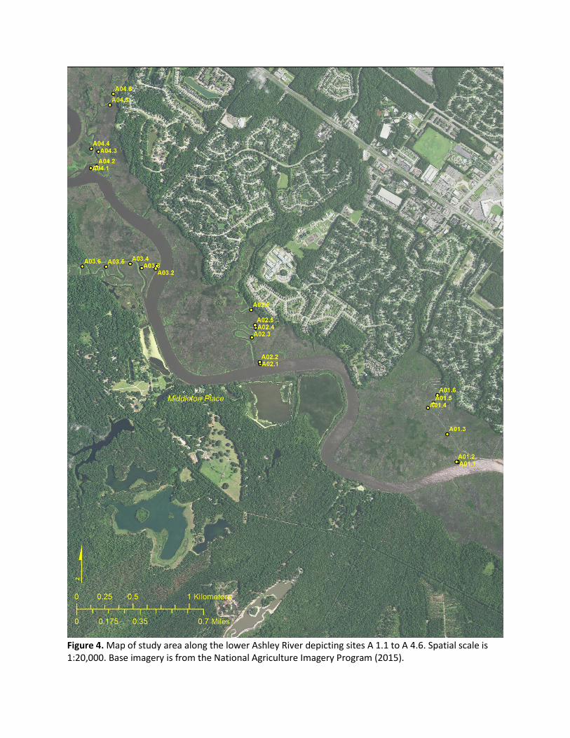
Figure 4. Map of study area along the lower Ashley River depicting sites A 1.1 to A 4.6. Spatial scale is 1:20,000. Base imagery is from the National Agriculture Imagery Program (2015).

Figure 5. Shade plot of relative percent cover for individual plant species by transect (midpoint of percent cover range, averaged across the 6 plots in each transect) along the Ashley River in Fall 2016. A black cell indicates high mean percent cover of a plant species in the plots within a transect, a lighter gray cell indicates lower mean percent cover, and a white cell indicates that a plant species was not observed in any plot in that transect. The dendrogram on the left shows groupings of plants with similar patterns of percent cover among transects; plant groups linked by horizontal black lines had significantly different distribution patterns relative to other groups. Porewater salinities (ppt) were pooled across seasons to represent within-year exposures.

Figure 6. Shade plot of relative percent cover for individual plant species by transect (midpoint of percent cover range, averaged across the 6 plots in each transect) along the Ashley River in Spring 2017. A black cell indicates high mean percent cover of a plant species in the plots within a transect, a lighter gray cell indicates lower mean percent cover, and a white cell indicates that a plant species was not observed in any plot in that transect. The dendrogram on the left shows groupings of plants with similar patterns of percent cover among transects; plant groups linked by horizontal black lines had significantly different distribution patterns relative to other groups. Porewater salinities (ppt) were pooled across seasons to represent within-year exposures.

Figure 7. Shade plot of relative percent cover for individual plant species by transect (midpoint of percent cover range, averaged across the 6 plots in each transect) along the Cooper River in Fall 2016. A black cell indicates high mean percent cover of a plant species in the plots within a transect, a lighter gray cell indicates lower mean percent cover, and a white cell indicates that a plant species was not observed in any plot in that transect. The dendrogram on the left shows groupings of plants with similar patterns of percent cover among transects; plant groups linked by horizontal black lines had significantly different distribution patterns relative to other groups. Porewater salinities (ppt) were pooled across seasons to represent within-year exposures.

Figure 8. Shade plot of relative percent cover for individual plant species by transect (midpoint of percent cover range, averaged across the 6 plots in each transect) along the Cooper River in Spring 2017. A black cell indicates high mean percent cover of a plant species in the plots within a transect, a lighter gray cell indicates lower mean percent cover, and a white cell indicates that a plant species was not observed in any plot in that transect. The dendrogram on the left shows groupings of plants with similar patterns of percent cover among transects; plant groups linked by horizontal black lines had significantly different distribution patterns relative to other groups. Porewater salinities (ppt) were pooled across seasons to represent within-year exposures.

Figure 9. Shade plot of relative percent cover for individual plant species by porewater salinity category, across both river systems and seasons. A black cell indicates high mean percent cover of a plant species in the plots, a lighter gray cell indicates lower mean percent cover, and a white cell indicates that a plant species was not observed in any plot in that porewater salinity category. The dendrogram on the left shows groupings of plants with similar patterns of percent cover among plots. Plant groups linked by horizontal black lines had significantly different distribution patterns relative to other groups. Each plot had two porewater salinity readings (fall and spring) and the higher value was used to categorize the porewater salinity category for each plot.

Figure 10. Species richness averaged by transect for Cooper River (dashed lines) and Ashley River (solid lines). Green lines indicate spring values and orange lines indicate fall values. Error bars depict standard error.

Figure 11. Porewater salinity averaged by transect for seasons (lines, Cooper: dashed, Ashley: solid). Bars depict seasonal variation, with the upper limits representing fall sampling and the lower limits representing spring sampling (except Cooper River transects 1 and 2 where spring salinities were higher).

0

2

4

6

8

10

12

14

16

18

20

1 2 3 4 5 6 7 8 9 10

Spec

ies

rich

nes

s

Transect

0.0

0.5

1.0

1.5

2.0

2.5

3.0

3.5

4.0

4.5

5.0

1 2 3 4 5 6 7 8 9 10

Po

rew

ater

sal

init

y (p

pt)

Transect

Figure 12. Soil organic matter percent, averaged by transect for the Ashley River (solid line) and Cooper River (dashed line). Error bars depict standard error.

Figure 13. Plot elevations averaged by transect for the Ashley River (solid line) and Cooper River (dashed line). Error bars depict standard error.

0

10

20

30

40

50

60

70

1 2 3 4 5 6 7 8 9 10

Soil

org

anic

mat

ter

(%)

Transect

0.0

0.1

0.2

0.3

0.4

0.5

0.6

0.7

0.8

0.9

1.0

1 2 3 4 5 6 7 8 9 10

Plo

t el

evat

ion

(m

eter

s)

Transect

Figure 14. Plot elevations relative to tidal frame, averaged by transect for the Ashley River (solid line) and Cooper River (dashed line). Error bars depict standard error. A value of zero indicates that plot elevation is equal to MLW at that site. A value of one indicates that plot elevation is equal to MHW at that site.

0.0

0.1

0.2

0.3

0.4

0.5

0.6

0.7

0.8

0.9

1.0

1 2 3 4 5 6 7 8 9 10

Tid

al p

osi

tio

n (

see

text

fo

r ex

pl.)

Transect

Figure 15. Non-metric multidimensional scaling (nMDS) plots showing the relative similarity and dissimilarity among transect-level plant communities along the Ashley River in Fall (A) and Spring (B). Groups of plant communities identified as being significantly different from other plant community groupings by the SIMPROF test are circled in black. Greater distances are associated with greater dissimilarity. On each plot, the blue vectors indicate the direction and magnitude of associations for selected normalized factors (porewater salinity, % organic matter in soil, tidal position, distance from creek edge, distance from upland, whether the creek was historically ditched, and species richness).

Figure 16. Non-metric multidimensional scaling (nMDS) plots showing the relative similarity (and dissimilarity) among transect-level plant communities along the Cooper River in Fall (A) and Spring (B). Groups of plant communities identified as being significantly different from other plant community groupings by the SIMPROF test are circled in black. Greater distances are associated with greater dissimilarity. On each plot, the blue vectors indicate the direction and magnitude of associations for selected normalized factors (porewater salinity, % organic matter in soil, tidal position, distance from creek edge, distance from upland, whether the creek was historically ditched, and species richness).

Table 1. Ashley River site locations, elevations (meters, converted from NAVD88) and elevations relative to site-specific tidal datums as calculated from VDATUM. Tidal position represents the elevation as a percentage of the tidal frame (MLW/(MLW-MHW)).

Plot_ID LatDD LongDD ElevRaw MLLW MLW MHW MHHW Tidal Position

A01.1 32.89376 -80.10746 0.86 1.57 1.51 -0.06 -0.15 0.96

A01.2 32.89378 -80.10757 0.89 1.60 1.55 -0.03 -0.12 0.98

A01.3 32.89600 -80.10840 0.73 1.44 1.39 -0.19 -0.29 0.88

A01.4 32.89812 -80.11023 0.68 1.38 1.33 -0.25 -0.35 0.84

A01.5 32.89850 -80.10970 0.66 1.36 1.31 -0.27 -0.36 0.83

A01.6 32.89914 -80.10931 0.72 1.42 1.37 -0.21 -0.30 0.87

A02.1 32.90177 -80.12615 0.65 1.24 1.19 -0.28 -0.37 0.81

A02.2 32.90192 -80.12618 0.64 1.23 1.18 -0.29 -0.38 0.80

A02.3 32.90390 -80.12690 0.83 1.42 1.37 -0.10 -0.19 0.93

A02.4 32.90467 -80.12653 0.78 1.36 1.31 -0.16 -0.25 0.89

A02.5 32.90488 -80.12659 0.68 1.26 1.21 -0.26 -0.35 0.83

A02.6 32.90610 -80.12696 0.70 1.28 1.24 -0.23 -0.32 0.84

A03.1 32.90969 -80.13588 0.68 1.19 1.15 -0.26 -0.35 0.81

A03.2 32.90947 -80.13600 0.48 1.00 0.96 -0.46 -0.55 0.68

A03.3 32.90953 -80.13733 0.59 1.11 1.07 -0.35 -0.44 0.75

A03.4 32.90988 -80.13841 0.61 1.12 1.08 -0.34 -0.43 0.76

A03.5 32.90965 -80.14072 0.69 1.20 1.16 -0.26 -0.35 0.81

A03.6 32.90970 -80.14297 0.52 1.03 0.98 -0.44 -0.53 0.69

A04.1 32.91758 -80.14210 0.90 1.37 1.33 -0.05 -0.14 0.96

A04.2 32.91772 -80.14153 0.68 1.14 1.10 -0.28 -0.36 0.80

A04.3 32.91890 -80.14136 0.80 1.25 1.21 -0.15 -0.24 0.89

A04.4 32.91914 -80.14203 0.60 1.05 1.01 -0.35 -0.44 0.74

A04.5 32.92263 -80.14021 0.64 1.08 1.03 -0.31 -0.40 0.77

A04.6 32.92352 -80.13989 0.77 1.21 1.17 -0.17 -0.26 0.87

A05.1 32.92537 -80.14958 0.83 1.22 1.18 -0.13 -0.22 0.90

A05.2 32.92550 -80.14873 0.78 1.17 1.13 -0.18 -0.27 0.86

A05.3 32.92722 -80.14754 0.78 1.17 1.13 -0.19 -0.27 0.86

A05.4 32.92770 -80.14744 0.78 1.17 1.13 -0.18 -0.27 0.86

A05.5 32.92804 -80.14702 0.81 1.20 1.16 -0.15 -0.24 0.89

A05.6 32.92874 -80.14668 0.86 1.25 1.21 -0.11 -0.19 0.92

A06.1 32.93347 -80.15471 0.68 1.00 0.97 -0.29 -0.37 0.77

A06.2 32.93388 -80.15490 0.72 1.04 1.00 -0.25 -0.34 0.80

A06.3 32.93396 -80.15500 0.77 1.09 1.06 -0.20 -0.28 0.84

A06.4 32.93420 -80.15509 0.75 1.07 1.03 -0.22 -0.31 0.82

A06.5 32.93446 -80.15513 0.71 1.03 0.99 -0.26 -0.34 0.79

A06.6 32.93439 -80.15540 0.75 1.06 1.02 -0.23 -0.31 0.82

A07.1 32.93843 -80.15629 0.48 0.77 0.73 -0.49 -0.58 0.60

A07.2 32.93851 -80.15634 0.79 1.07 1.04 -0.19 -0.27 0.85

A07.3 32.93859 -80.15656 0.87 1.15 1.11 -0.11 -0.19 0.91

A07.4 32.93890 -80.15629 0.88 1.17 1.13 -0.09 -0.17 0.93

A07.5 32.93900 -80.15645 0.82 1.10 1.06 -0.16 -0.24 0.87

A07.6 32.93929 -80.15640 1.02 1.30 1.26 0.04 -0.04 1.04

A08.1 32.94156 -80.15670 0.66 0.92 0.88 -0.31 -0.40 0.74

A08.2 32.94193 -80.15689 0.58 0.84 0.80 -0.39 -0.47 0.67

A08.3 32.94196 -80.15728 0.12 0.38 0.34 -0.85 -0.93 0.29

A08.4 32.94222 -80.15728 0.65 0.91 0.87 -0.32 -0.40 0.73

A08.5 32.94234 -80.15737 0.77 1.02 0.99 -0.20 -0.29 0.83

A08.6 32.94204 -80.15757 0.75 1.00 0.97 -0.22 -0.31 0.81

A09.1 32.94530 -80.16215 0.75 0.95 0.91 -0.23 -0.32 0.80

A09.2 32.94538 -80.16221 0.76 0.96 0.93 -0.22 -0.30 0.81

A09.3 32.94506 -80.16249 0.80 1.00 0.97 -0.18 -0.26 0.85

A09.4 32.94486 -80.16256 0.80 1.00 0.97 -0.18 -0.26 0.85

A09.5 32.94474 -80.16279 0.80 0.99 0.96 -0.18 -0.27 0.84

A09.6 32.94450 -80.16267 0.75 0.95 0.92 -0.23 -0.31 0.80

A10.1 32.94715 -80.17144 0.69 0.79 0.76 -0.29 -0.37 0.72

A10.2 32.94705 -80.17184 0.73 0.82 0.79 -0.24 -0.32 0.76

A10.3 32.94724 -80.17185 0.71 0.80 0.77 -0.27 -0.34 0.74

A10.4 32.94698 -80.17225 0.81 0.88 0.85 -0.16 -0.24 0.84

A10.5 32.94746 -80.17202 0.71 0.79 0.76 -0.27 -0.35 0.74

A10.6 32.94755 -80.17224 0.75 0.82 0.80 -0.22 -0.30 0.78

Table 2. Cooper River site locations, elevations (meters, converted from NAVD88) and elevations relative to site-specific tidal datums as calculated from VDATUM. Tidal position represents the elevation as a percentage of the tidal frame (MLW/(MLW-MHW)).

Plot_ID LatDD LongDD ElevRaw MLLW MLW MHW MHHW Tidal Position

C01.1 32.97923 -79.91283 0.73 1.49 1.43 -0.03 -0.12 0.98

C01.2 32.97925 -79.91320 0.67 1.43 1.37 -0.09 -0.19 0.94

C01.3 32.97983 -79.91691 0.48 1.23 1.17 -0.27 -0.36 0.81

C01.4 32.98018 -79.91771 0.55 1.30 1.24 -0.19 -0.29 0.87

C01.5 32.98047 -79.91982 0.32 1.07 1.01 -0.42 -0.52 0.70

C01.6 32.97916 -79.92252 0.55 1.33 1.27 -0.23 -0.32 0.85

C02.1 32.97827 -79.90889 0.37 1.13 1.07 -0.39 -0.49 0.73

C02.2 32.97825 -79.90879 0.61 1.37 1.31 -0.16 -0.25 0.89

C02.3 32.98107 -79.90387 0.64 1.39 1.33 -0.14 -0.23 0.91

C02.4 32.98160 -79.90353 0.60 1.34 1.28 -0.18 -0.28 0.88

C02.5 32.98376 -79.90087 0.60 1.34 1.28 -0.18 -0.28 0.88

C02.6 32.98428 -79.90058 0.65 1.39 1.33 -0.13 -0.22 0.91

C03.1 32.99625 -79.90679 0.63 1.29 1.23 -0.12 -0.21 0.91

C03.2 32.99608 -79.90629 0.58 1.24 1.18 -0.18 -0.26 0.87

C03.3 32.99481 -79.90293 0.57 1.23 1.17 -0.19 -0.28 0.86

C03.4 32.99523 -79.90242 0.51 1.17 1.11 -0.25 -0.33 0.82

C03.5 32.99444 -79.90084 0.67 1.33 1.26 -0.09 -0.18 0.93

C03.6 32.99372 -79.90004 0.66 1.32 1.26 -0.10 -0.19 0.93

C04.1 33.01129 -79.90231 0.63 1.24 1.17 -0.16 -0.25 0.88

C04.2 33.01191 -79.90209 0.68 1.29 1.23 -0.11 -0.19 0.92

C04.3 33.01231 -79.90161 0.70 1.31 1.25 -0.08 -0.17 0.94

C04.4 33.01474 -79.90094 0.66 1.24 1.18 -0.13 -0.21 0.90

C04.5 33.01507 -79.90034 0.65 1.23 1.16 -0.14 -0.22 0.90

C04.6 33.01597 -79.89948 0.54 1.12 1.05 -0.25 -0.33 0.81

C05.1 33.02136 -79.91852 0.69 1.20 1.14 -0.06 -0.15 0.95

C05.2 33.02145 -79.91885 0.71 1.22 1.16 -0.04 -0.13 0.96

C05.3 33.02159 -79.92108 0.34 0.85 0.79 -0.42 -0.50 0.65

C05.4 33.02177 -79.92109 0.56 1.07 1.01 -0.19 -0.28 0.84

C05.5 33.02239 -79.92493 0.52 1.04 0.97 -0.23 -0.31 0.81

C05.6 33.02251 -79.92523 0.57 1.09 1.02 -0.18 -0.26 0.85

C06.1 33.03844 -79.92342 0.72 1.11 1.04 -0.07 -0.15 0.94

C06.2 33.03551 -79.92423 0.44 0.84 0.77 -0.34 -0.42 0.70

C06.3 33.03413 -79.92639 0.68 1.07 1.01 -0.10 -0.18 0.91

C06.4 33.03086 -79.92588 0.69 1.08 1.02 -0.09 -0.17 0.92

C06.5 33.02993 -79.92565 0.69 1.09 1.02 -0.08 -0.16 0.93

C06.6 33.02894 -79.92580 0.59 0.99 0.92 -0.18 -0.26 0.83

C07.1 33.04048 -79.91731 0.76 1.15 1.09 -0.04 -0.12 0.96

C07.2 33.04282 -79.91595 0.61 1.00 0.94 -0.19 -0.27 0.83

C07.3 33.04468 -79.91582 0.71 1.09 1.02 -0.11 -0.19 0.91

C07.4 33.04656 -79.91597 0.67 1.04 0.98 -0.15 -0.23 0.87

C07.5 33.04753 -79.91528 0.67 1.04 0.97 -0.16 -0.24 0.86

C07.6 33.04809 -79.91531 0.51 0.88 0.82 -0.31 -0.39 0.72

C08.1 33.05890 -79.92615 0.43 0.65 0.59 -0.35 -0.43 0.62

C08.2 33.05918 -79.92749 0.38 0.59 0.53 -0.41 -0.48 0.56

C08.3 33.05958 -79.92835 0.34 0.54 0.47 -0.45 -0.52 0.51

C08.4 33.06041 -79.92880 0.27 0.46 0.39 -0.50 -0.58 0.44

C08.5 33.06136 -79.92982 0.37 0.54 0.48 -0.41 -0.48 0.54

C08.6 33.06156 -79.93115 0.43 0.59 0.53 -0.35 -0.42 0.60

C09.1 33.06488 -79.90091 0.54 0.74 0.67 -0.21 -0.28 0.77

C09.2 33.06370 -79.90326 0.54 0.74 0.67 -0.21 -0.28 0.76

C09.3 33.06362 -79.90318 0.63 0.83 0.77 -0.12 -0.19 0.87

C09.4 33.06333 -79.90404 0.59 0.80 0.73 -0.16 -0.23 0.82

C09.5 33.06169 -79.90796 0.61 0.82 0.75 -0.14 -0.21 0.85

C09.6 33.06134 -79.90799 0.57 0.78 0.71 -0.18 -0.25 0.80

C10.1 33.06756 -79.93842 0.44 0.55 0.49 -0.35 -0.43 0.58

C10.2 33.06805 -79.93999 0.05 0.15 0.09 -0.75 -0.83 0.10

C10.3 33.06878 -79.94146 0.40 0.50 0.44 -0.41 -0.48 0.52

C10.4 33.06943 -79.94222 0.55 0.64 0.58 -0.26 -0.33 0.69

C10.5 33.06948 -79.94347 0.45 0.54 0.48 -0.36 -0.44 0.57

C10.6 33.06934 -79.94356 0.57 0.66 0.60 -0.24 -0.31 0.72

Table 3. List of plant species identified in Ashley and Cooper River study plots.

Plant species Plant species, cont.

Acer rubrum Oxypolis filiformis

Alternanthera philoxeroides Panicum sp.

Amaranthus cannabinus Peltandra virginica

Ampelaster carolinianus Persicaria arifolia OR sagittattum

Apios americana Phyla lanceolata

Bacopa sp. Physostegia leptophylla

Bidens laevis Pluchea carolinensis

Bolboschoenus robustus Poaceae

Carex sp. Polygonum sp.

Cicuta maculata Pontederia cordata

Cladium jamaicense Ptilimnium capillaceum

Colocasia esculenta Ptilimnium sp.

Cuscuta sp. Ranunculus sceleratus var sceleratus

Cyperus odoratus Rosa palustris

Cyperus sp. Rumex sp.

Eleocharis sp. Rumex verticillatus

Eryngium aquaticum Sacciolepis striata

Galium obtusum Sagittaria graminea

Galium sp. Sagittaria lancifolia

Hymenocallis crassifolia Sagittaria latifolia

Hypericum mutilum Sagittaria subulata

Impatiens capensis Saururus cernuus

Ipomoea sagittata Schoenoplectus americanus

Juncus canadensis Schoenoplectus tabernaemontani

Juncus effusus Sesbania punicea

Juncus roemerianus Sium suave

Juncus sp. Spartina alterniflora

Kosteletzkya pentacarpos Spartina cynosuroides

Limnobium spongia Symphyotrichum puniceum

Lippia sp. Symphyotrichum tenuifolium

Lobelia elongata Thelypteris sp.

Ludwigia sp. Toxicodendron radicans

Lycopus sp. Triadenum walteri

Lythrum lineare Typha angustifolia

Mikania scandens Typha latifolia

Murdannia keisak Zizania aquatica

Nyssa biflora Zizaniopsis miliacea

Onoclea sensibilis

Table 4. Multiple regression results for model of species richness as explained by four independent variables. Porewater values were log-transformed to reduce skew of the residuals.

Table 5. Species-specific stepwise multiple regression models for species exhibiting changes in abundance near the oligohaline-tidal freshwater transition zone. Independent variable values are p values. Parenthetical notes indicate the relationship between species abundance and each variable.

Full Model: Species Richness

Dependent r F p n

Species richness 0.51 61.07 <0.0001 240

Independent estimate t ratio p Notes

Intercept 1.0001 0.69 0.4933

Season -0.4875 -2.41 0.0169 Spring > Fall

Mean pw salinity (log) -1.7811 -6.75 <0.0001 More species at lower salinity

River -1.9241 -7.95 <0.0001 Cooper > Ashley

Tidal position 8.6471 5.10 <0.0001 More species at higher position

Species Models r 2 p

Porewater

salinity

(log)

Tidal

position

Distance

to upland

Distance

to edge

Soil

organic

matter Season River Ditched

Cicuta maculata 0.25 <0.0001 <0.0001 (-) 0.0030 (+) <0.0001 (s>f)

Juncus roemerianus 0.31 <0.0001 <0.0001 (+) 0.0001 (+)

Ludwigia sp. 0.17 <0.0001 <0.0001 (C>A)

Lythrum lineare 0.21 <0.0001 <0.0001 (+) 0.0092 (-) 0.0050 (+) 0.0002 (f>s) <0.0001 (C>A)

Peltandra virginica 0.38 <0.0001 <0.0001 (C>A) <0.0001 (y>n)

Schoenoplectus americanus 0.11 <0.0001 0.0005 (+) <0.0001 (C>A)

Thelypteris sp. 0.24 <0.0001 <0.0001 (-) <0.0001 (+) 0.0186 (-)

Typha latifolia 0.04 0.0012 0.0012 (A>C)

Zizaniopsis miliacea 0.31 <0.0001 0.0332 (-) 0.0008 (-) 0.0002 (+) 0.0011 (+) 0.0018 (y>n)