charalampos e. tsourakakis richard peng maria a. …

39

Approximation Algorithms for Speeding up Dynamic Programmingand Denoising aCGH data

CHARALAMPOS E. TSOURAKAKIS, Carnegie Mellon UniversityRICHARD PENG, Carnegie Mellon UniversityMARIA A. TSIARLI, University of PittsburghGARY L. MILLER, Carnegie Mellon UniversityRUSSELL SCHWARTZ, Carnegie Mellon University

The development of cancer is largely driven by the gain or loss of subsets of the genome, promoting uncon-trolled growth or disabling defenses against it. Denoising array-based Comparative Genome Hybridization(aCGH) data is an important computational problem central to understanding cancer evolution. In thiswork we propose a new formulation of the denoising problem which we solve with a “vanilla” dynamic pro-gramming algorithm which runs in O(n2) units of time. Then, we propose two approximation techniques.Our first algorithm reduces the problem into a well-studied geometric problem, namely halfspace emptiness

queries, and provides an ε additive approximation to the optimal objective value in O(n43+δ log (U

ε)) time,

where δ is an arbitrarily small positive constant and U = max{√C, (|Pi|)i=1,...,n} (P = (P1, P2, . . . , Pn),

Pi ∈ R, is the vector of the noisy aCGH measurements, C a normalization constant). The second algorithmprovides a (1±ε) approximation (multiplicative error) and runs in O(n logn/ε) time. The algorithm decom-poses the initial problem into a small (logarithmic) number of Monge optimization subproblems which wecan solve in linear time using existing techniques.

Finally, we validate our model on synthetic and real cancer datasets. Our method consistently achievessuperior precision and recall to leading competitors on the data with ground truth. In addition, it findsseveral novel markers not recorded in the benchmarks but supported in the oncology literature.

Availability: Code, datasets and results available from the first author’s web page http://www.math.

cmu.edu/~ctsourak/DPaCGHsupp.html.

Categories and Subject Descriptors: F.2.1 [Analysis of Algorithms and Problem Complexity]: Numer-ical Algorithms and Problems; G.2.1 [Combinatorics]: Combinatorial Algorithms; J.3 [Life and MedicalSciences]: Biology and genetics

General Terms: Algorithms, Experimentation

Additional Key Words and Phrases: Approximation algorithms, dynamic programming, halfspace rangequeries, computational biology, denoising aCGH data, time series segmentation

C.E.T was supported in this work by NSF grant ccf1013110 and by U.S. National Institute of Health award1R01CA140214. R.P. was supported in this work by Natural Sciences and Engineering Research Council ofCanada (NSERC), under Grant PGS M-377343-2009. G.L.M. was supported in this work by the National Sci-ence Foundation under Grant No. CCF-0635257. R.S. was supported in this work by U.S. National Instituteof Health award 1R01CA140214. Any opinions, findings, and conclusions or recommendations expressed inthis material are those of the author(s) and do not necessarily reflect the views of the National Institute ofHealth and National Science Foundation, or other funding parties.Author’s addresses: C.E. Tsourakakis, Department of Mathematical Sciences, Carnegie Mellon University;R. Peng, School of Computer Science, Carnegie Mellon University; M. Tsiarli, Center for Neuroscience, Uni-versity of Pittsburgh; G.L. Miller, School of Computer Science, Carnegie Mellon University; R. Schwartz,Department of Biological Sciences and School of Computer Science, Carnegie Mellon University.Permission to make digital or hard copies of part or all of this work for personal or classroom use is grantedwithout fee provided that copies are not made or distributed for profit or commercial advantage and thatcopies show this notice on the first page or initial screen of a display along with the full citation. Copyrightsfor components of this work owned by others than ACM must be honored. Abstracting with credit is per-mitted. To copy otherwise, to republish, to post on servers, to redistribute to lists, or to use any componentof this work in other works requires prior specific permission and/or a fee. Permissions may be requestedfrom Publications Dept., ACM, Inc., 2 Penn Plaza, Suite 701, New York, NY 10121-0701 USA, fax +1 (212)869-0481, or [email protected]© 2011 ACM 1084-6654/2011/03-ART39 $10.00

DOI 10.1145/0000000.0000000 http://doi.acm.org/10.1145/0000000.0000000

ACM Journal of Experimental Algorithmics, Vol. 9, No. 4, Article 39, Publication date: March 2011.

39:2 C.E. Tsourakakis et. al.

ACM Reference Format:Tsourakakis C.E., Peng R., Tsiarli M.A., Miller G.L., Schwartz R. 2011. Approximation Algorithms for Speed-ing up Dynamic Programming and Denoising aCGH data. ACM J. Exp. Algor. 9, 4, Article 39 (March 2011),27 pages.DOI = 10.1145/0000000.0000000 http://doi.acm.org/10.1145/0000000.0000000

1. INTRODUCTIONTumorigenesis is a complex phenomenon often characterized by the successive acqui-sition of combinations of genetic aberrations that result in malfunction or disregula-tion of genes. There are many forms of chromosome aberration that can contribute tocancer development, including polyploidy, aneuploidy, interstitial deletion, reciprocaltranslocation, non-reciprocal translocation, as well as amplification, again with severaldifferent types of the latter (e.g., double minutes, HSR and distributed insertions [Al-bertson and Pinkel 2003]). Identifying the specific recurring aberrations, or sequencesof aberrations, that characterize particular cancers provides important clues aboutthe genetic basis of tumor development and possible targets for diagnostics or thera-peutics. Many other genetic diseases are also characterized by gain or loss of geneticregions, such as Down Syndrome (trisomy 21) [Lejeune et al. 1959], Cri du Chat (5pdeletion) [Lejeune et al. 1963], and Prader-Willi syndrome (deletion of 15q11-13) [But-ler et al. 1986] and recent evidence has begun to suggest that inherited copy numbervariations are far more common and more important to human health than had beensuspected just a few years ago [Zhang et al. 2009]. These facts have created a need formethods for assessing DNA copy number variations in individual organisms or tissues.

In this work, we focus specifically on array-based comparative genomic hybridization(aCGH) [Bignell et al. 2004; Pollack et al. 1999; Kallioniemi et al. 1992; Pinkel et al.1998], a method for copy number assessment using DNA microarrays that remains,for the moment, the leading approach for high-throughput typing of copy number ab-normalities. The technique of aCGH is schematically represented in Figure 1. A testand a reference DNA sample are differentially labeled and hybridized to a microarrayand the ratios of their fluorescence intensities is measured for each spot. A typical out-put of this process is shown in Figure 1 (3), where the genomic profile of the cell lineGM05296 [Snijders et al. 2001] is shown for each chromosome. The x-axis correspondsto the genomic position and the y-axis corresponds to a noisy measurement of the ra-tio log2

TR for each genomic position, typically referred to as “probe” by biologists. For

healthy diploid organisms, R=2 and T is the DNA copy number we want to infer fromthe noisy measurements. For more details on the use of aCGH to detect different typesof chromosomal aberrations, see [Albertson and Pinkel 2003].

Converting raw aCGH log fluorescence ratios into discrete DNA copy numbers isan important but non-trivial problem. Finding DNA regions that consistently exhibitchromosomal losses or gains in cancers provides a crucial means for locating the spe-cific genes involved in development of different cancer types. It is therefore importantto distinguish, when a probe shows unusually high or low fluorescence, whether thataberrant signal reflects experimental noise or a probe that is truly found in a segmentof DNA that is gained or lost. Furthermore, successful discretization of array CGHdata is crucial for understanding the process of cancer evolution, since discrete inputsare required for a large family of successful evolution algorithms, e.g., [Desper et al.1999; 2000]. It is worth noting that manual annotation of such regions, even if possible[Snijders et al. 2001], is tedious and prone to mistakes due to several sources of noise(impurity of test sample, noise from array CGH method, etc.).

Based on the well-established observation that near-by probes tend to have the sameDNA copy number, we formulate the problem of denoising aCGH data as the problem ofapproximating a signal P with another signal F consisting of a few piecewise constant


Approximation Algorithms for Speeding up Dynamic Programming and denoising aCGH data 39:3

Fig. 1. Schematic representation of array CGH. Genomic DNA from two cell populations (1) is differentiallylabeled and hybridized in a microarray (2). Typically the reference DNA comes from a normal subject. Forhumans this means that the reference DNA comes from a normal diploid genome. The ratios on each spotare measured and normalised so that the median log2 ratio is zero. The final result is an ordered tuplecontaining values of the fluorescent ratios in each genomic position per each chromosome. This is shownin (3) where we see the genomic profile of the cell line GM05296 [Snijders et al. 2001]. The problem ofdenoising array CGH data is to infer the true DNA copy number T per genomic position from a set of noisymeasurements of the quantity log2

TR

, where R=2 for normal diploid humans.

segments. Specifically, let P = (P1, P2, . . . , Pn) ∈ Rn be the input signal -in our settingthe sequence of the noisy aCGH measurements- and let C be a constant. Our goal is tofind a function F : [n]→ R which optimizes the following objective function:

minF

n∑i=1

(Pi − Fi)2 + C × (|{i : Fi 6= Fi+1}|+ 1). (1)

The best known exact algorithm for solving the optimization problem defined byEquation 1 runs in O(n2) time but as our results suggest this running time is likelynot to be tight. It is worth noting that existing techniques for speeding up dynamicprogramming [Yao 1982; Eppstein et al. 1988; Eppstein et al. 1992a] do not apply toour problem. In this work, we provide two approximation algorithms for solving thisrecurrence. The first algorithm approximates the objective within an additive error εwhich we can make as small as we wish and its key idea is the reduction of the problemto halfspace range queries, a well studied computational geometric problem [Agarwaland Erickson 1999]. The second algorithm carefully decomposes the problem into a“small” (logarithmic) number of subproblems which satisfy the quadrangle inequality(Monge property). The main contributions of this work can be summarized as follows.

— We propose a new formulation of the aCGH denoising problem which we solve usinga dynamic programming algorithm in O(n2) time.

— We provide a technique which approximates the optimal value of our objective func-tion within additive ε error and runs in O(n

43 +δ log (Uε )) time, where δ is an arbitrarily

small positive constant and U = max{√C, (|Pi|)i=1,...,n}.

— We provide a technique for approximate dynamic programming which solves the cor-responding recurrence within a multiplicative factor of (1+ε) and runs in O(n log n/ε).



— We validate our proposed model on both synthetic and real data. Specifically, our seg-mentations result in superior precision and recall compared to leading competitorson benchmarks of synthetic data and real data from the Coriell cell lines. In addi-tion, we are able to find several novel markers not recorded in the benchmarks butsupported in the oncology literature.

The remainder of this paper is organized as follows: Section 2 briefly presents therelated work. Section 3 presents the vanilla dynamic programming algorithm whichruns in O(n2). Section 4 analyzes properties of the recurrence which will be exploitedin Sections 5 and 6 where we describe the additive and multiplicative approximationalgorithms respectively. In Section 7 we validate our model by performing an exten-sive biological analysis of the findings of our segmentation. Finally, in Section 8 weconclude.

2. RELATED WORKIn Section 2.1, we provide a brief overview of the existing work on the problem ofdenoising aCGH data. In Section 2.2, we present existing techniques for speeding updynamic programming and in Section 2.3 we discuss the problem of reporting pointsin halfspaces.

2.1. Denoising aCGH dataMany algorithms and objective functions have been proposed for the problem of dis-cretizing and segmenting aCGH data. Many methods, starting with [Fridlyand et al.2004], treat aCGH segmentation as a hidden Markov model (HMM) inference prob-lem. The HMM approach has since been extended in various ways, e.g., through theuse of Bayesian HMMs [Guha et al. 2006], incorporation of prior knowledge of loca-tions of DNA copy number polymorphisms [Shah et al. 2006], and the use of Kalmanfilters [Shi et al. 2007]. Other approaches include wavelet decompositions [Hsu et al.2005], quantile regression [Eilers and de Menezes 2005], expectation-maximization incombination with edge-filtering [Myers et al. 2004], genetic algorithms [Jong et al.2004], clustering-based methods [Xing et al. 2007; Wang et al. 2005], variants onLasso regression [Tibshirani and Wang 2008; Huang et al. 2005], and various problem-specific Bayesian [Barry and Hartigan 1993], likelihood [Hupe et al. 2004], and otherstatisical models [Lipson et al. 2005]. A dynamic programming approach, in combina-tion with expectation maximimization, has been previously used by Picard et al. [Pi-card et al. 2007]. In [Lai et al. 2005] and [Willenbrock and Fridlyand 2005] an ex-tensive experimental analysis of available methods has been conducted. Two methodsstand out as the leading approaches in practice. One of these top methods is CGHSEG[Picard et al. 2005], which assumes that a given CGH profile is a Gaussian processwhose distribution parameters are affected by abrupt changes at unknown coordi-nates/breakpoints. The other method which stands out for its performance is CircularBinary Segmentation [Olshen et al. 2004] (CBS), a modification of binary segmenta-tion, originally proposed by Sen and Srivastava [Sen and Srivastava 1975], which usesa statistical comparison of mean expressions of adjacent windows of nearby probes toidentify possible breakpoints between segments combined with a greedy algorithm tolocally optimize breakpoint positions.

2.2. Speeding up Dynamic ProgrammingDynamic programming is a powerful problem solving technique introduced by Bell-man [Bellman 2003] with numerous applications in biology, e.g., [Picard et al. 2005;Hirschberg 1975; Waterman and Smith 1986], in control theory, e.g., [Bertsekas 2000],in operations research and many other fields. Due to its importance, a lot of re-



search has focused on speeding up basic dynamic programming implementations. Asuccessful example of speeding up a naive dynamic programming implementation isthe computation of optimal binary search trees. Gilbert and Moore solved the prob-lem efficiently using dynamic programming [Gilbert and Moore 1959]. Their algo-rithm runs in O(n3) time and for several years this running time was considered tobe tight. In 1971 Knuth [Knuth 1971] showed that the same computation can be car-ried out in O(n2) time. This remarkable result was generalized by Frances Yao in [Yao1982; 1980]. Specifically, Yao showed that this dynamic programming speedup tech-nique works for a large class of recurrences. She considered the recurrence c(i, i) = 0,c(i, j) = mini<k≤j (c(i, k − 1) + c(k, j))+w(i, j) for i < j where the weight function w sat-isfies the quadrangle inequality (see Section 2.4) and proved that the solution of thisrecurrence can be found in O(n2) time. Eppstein, Galil and Giancarlo have consideredsimilar recurrences where they showed that naive O(n2) implementations of dynamicprogramming can run in O(n log n) time [Eppstein et al. 1988]. Larmore and Schieber[Larmore and Schieber 1991] further improved the running time, giving a linear timealgorithm when the weight function is concave. Klawe and Kleitman give in [Klaweand Kleitman 1990] an algorithm which runs in O(nα(n)) time when the weight func-tion is convex, where α(·) is the inverse Ackermann function. Furthermore, Eppstein,Galil, Giancarlo and Italiano have also explored the effect of sparsity [Eppstein et al.1992a; 1992b], another key concept in speeding up dynamic programming. Aggarwal,Klawe, Moran, Shor, Wilber developed an algorithm, widely known as the SMAWKalgorithm, [Aggarwal et al. 1986] which can compute in O(n) time the row maximaof a totally monotone n × n matrix. The connection between the Knuth-Yao techniqueand the SMAWK algorithm was made clear in [Bein et al. 2009], by showing that theKnuth-Yao technique is a special case of the use of totally monotone matrices. The ba-sic properties which allow these speedups are the convexity or concavity of the weightfunction. Such properties date back to Monge [Monge 1781] and are well studied in theliterature, see for example [Burkard et al. 1996].

Close to our work lies the work on histogram construction, an important problemfor database applications. Jagadish et al. [Jagadish et al. 1998] originally provided asimple dynamic programming algorithm which runs in O(kn2) time, where k is thenumber of buckets and n the input size and outputs the best V-optimal histogram.Guha, Koudas and Shim [Guha et al. 2006] propose a (1 + ε) approximation algorithmwhich runs in linear time. Their algorithms exploits monotonicity properties of the keyquantities involved in the problem. Our (1 + ε) approximation algorithm in Section 2.4uses a decomposition technique similar to theirs.

2.3. Reporting Points in a HalfspaceLet S be a set of points in Rd and let k denote the size of the output, i.e., the num-ber of points to be reported. Consider the problem of preprocessing S such that forany halfspace query γ we can report efficiently whether the set S ∩ γ is empty or not.This problem is a well studied special case of the more general range searching prob-lem. For an extensive survey see the work by Agarwal and Erickson [Agarwal andErickson 1999]. For d = 2, the problem has been solved optimally by Chazelle, Guibasand Lee [Chazelle et al. 1985]. For d = 3, Chazelle and Preparata in [Chazelle andPreparata 1985] gave a solution with nearly linear space and O(log n+ k) query time,while Aggarwal, Hansen and Leighton [Aggarwal et al. 1990] gave a solution with amore expensive preprocessing but O(n log n) space. When the number of dimensionsis greater than 4, i.e., d ≥ 4, Clarkson and Shor [Clarkson and Shor. 1989] gave analgorithm that requires O(nbd/2c+ε) preprocessing time and space, where ε is an arbi-trarily small positive constant, but can subsequently answer queries in O(log n + k)time. Matousek in [Matousek 1991] provides improved results on the problem, which



are used by Agarwal, Eppstein, Matousek [Agarwal et al. 1992] in order to create dy-namic data structures that trade off insertion and query times. We refer to Theorem2.1(iii) of their paper [Agarwal et al. 1992]:

THEOREM 2.1 (AGARWAL, EPPSTEIN, MATOUSEK [AGARWAL ET AL. 1992]).Given a set S of n points in Rd where d ≥ 3 and a parameter m between n andnb

d2 c the halfspace range reporting problem can be solved with the following perfor-

mance: O( nm1/bd/2c log n) query time, O(m1+ε) space and preprocessing time, O(m1+ε/n)

amortized update time.

Substituting for d = 4, m = n43 we obtain the following corollary, which will be used

as a subroutine in our proposed method:

COROLLARY 2.2. Given a set S of n points in R4 the halfspace range reporting prob-lem can be solved with O(n

13 log n) query time, O(n

43 +δ) space and preprocessing time,

and O(n13 +δ) update time, where δ is an arbitrarily small positive constant.

2.4. Monge Functions and Dynamic ProgrammingHere, we refer to one of the results in [Larmore and Schieber 1991] which we use inSection 2.4 as a subroutine for our proposed method. A function w defined on pairsof integer indices is Monge (concave) if for any 4-tuple of indices i1 < i2 < i3 < i4,w(i1, i4) + w(i2, i3) ≥ w(i1, i3) + w(i2, i4). Furthermore, we assume that f is a functionsuch that the values f(aj) for all j are easily evaluated. The following results holds:

THEOREM 2.3 ([LARMORE AND SCHIEBER 1991]). Consider the one dimensionalrecurrence ai = minj<i{f(aj) + w(j, i)} for i = 1, . . . , n, where the basis a0 is given.There exists an algorithm which solves the recurrence online in O(n) time1.

3. O(N2) DYNAMIC PROGRAMMING ALGORITHMIn order to solve the optimization problem defined by Equation 1, we define the keyquantity OPTi given by the following recurrence:

OPT0 = 0OPTi = min

0≤j≤i−1[OPTj + w(i, j)] + C, for i > 0

where w(i, j) =i∑

k=j+1

(Pk −

∑im=j+1 Pm

i− j

)2

.

The above recurrence has a straightforward interpretation: OPTi is equal to theminimum cost of fitting a set of piecewise constant segments from point P1 to Pi giventhat index j is a breakpoint. The cost of fitting the segment from j + 1 to i is C. Theweight function w() is the minimum squared error for fitting a constant segment on

points {Pj+1, . . . , Pi}, which is obtained for the constant segment with valuePi

m=j+1 Pm

i−j ,i.e., the average of the points in the segment. This recursion directly implies a simpledynamic programming algorithm. We call this algorithm CGHTRIMMER and the pseu-docode is shown in Algorithm 1. The main computational bottleneck of CGHTRIMMERis the computation of the auxiliary matrix M , an upper diagonal matrix for which mij

1Thus, obtaining O(n) speedup compared to the straight-forward dynamic programming algorithm whichruns in O(n2) units of time.



is the minimum squared error of fitting a segment from points {Pi, . . . , Pj}. To avoid anaıve algorithm that would simply find the average of those points and then computethe squared error, resulting in O(n3) time, we use Claim 1.

ALGORITHM 1: CGHTRIMMER algorithmInput: Signal P = (P1, . . . , Pn), Regularization parameter COutput: Optimal Segmentation with respect to our objective (see Equation 1)

/* Compute an n× n matrix M, where Mji =Pik=j

„Pk −

Pim=j Pm

i−j+1

«2

. */

/* A is an auxiliary matrix of averages, i.e., Aji =Pi

k=j Pk

i−j+1. */

Initialize matrix A ∈ Rn×n, Aij = 0, i 6= j and Aii = Pi.for i = 1 to n do

for j = i+ 1 to n doAi,j ← j−i

j−i+1Ai,j−1 + 1

j−i+1Pj

endendfor i = 1 to n do

for j = i+ 1 to n doMi,j ←Mi,j−1 + j−i

j−i+1(Pj −Ai,j−1)

2

endend/* Solve the Recurrence. */for i = 1 to n do

OPTi ← min0≤j≤i−1OPTj +Mj+1,i + CBREAKi ← arg min1≤j≤iOPTj−1 +Mj,i + C

end

CLAIM 1. Let α(j) andm(j) be the average and the minimum squared error of fittinga constant segment to points {P1, . . . , Pj} respectively. Then,

α(j) =j − 1j

α(j−1) +1jPj , (2)

m(j) = m(j−1) +j − 1j

(Pj − α(j−1))2. (3)

The interested reader can find a proof of Claim 1 in [Knuth 1981]. Equations 2 and 3provide us a way to compute means and least squared errors online. Algorithm 1 firstcomputes matrices A and M using Equations 2, 3 and then iterates (last for loop) tosolve the recurrence by finding the optimal breakpoint for each index i. The total run-ning time is O(n2) (matrices A and M matrices have O(n2) entries and each requiresO(1) time to compute). Obviously, Algorithm 1 uses O(n2) units of space.

4. ANALYSIS OF THE TRANSITION FUNCTIONIn the following, let Si =

∑ij=1 Pj . The transition function for the dynamic program-

ming for i > 0 can be rewritten as:

OPTi = minj<i

OPTj +i∑

m=j+1

P 2m −

(Si − Sj)2

i− j+ C. (4)



The transition can be viewed as a weight function w(j, i) that takes the two indicesj and i as parameters such that:

w(j, i) =i∑

m=j+1

P 2m −

(Si − Sj)2

i− j+ C (5)

Note that the weight function does not have the Monge property, as demonstratedby the vector P = (P1, . . . , P2k+1) = (1, 2, 0, 2, 0, 2, 0, . . . 2, 0, 1). When C = 1, the optimalchoices of j for i = 1, . . . , 2k are j = i − 1, i.e., we fit one segment per point. However,once we add in P2k+1 = 1 the optimal solution changes to fitting all points on a singlesegment. Therefore, preferring a transition to j1 over one to j2 at some index i does notallow us to discard j2 from future considerations. This is one of the main difficultiesin applying techniques based on the increasing order of optimal choices of j, such asthe method of Eppstein, Galil and Giancarlo [Eppstein et al. 1988] or the method ofLarmore and Schieber [Larmore and Schieber 1991], to reduce the complexity of theO(n2) algorithm we described in Section 3.

We start by defining DPi for i = 0, 1, .., n, the solution to a simpler optimizationproblem.

Definition 4.1. Let DPi, i = 0, 1, .., n, satisfy the following recurrence

DPi =

{minj<iDPj − (Si−Sj)2

i−j + C if i > 00 if i = 0

(6)

The following observation stated as Lemma 4.2 plays a key role in Section 5.

LEMMA 4.2. For all i, OPTi can be written in terms of DPi as

OPTi = DPi +i∑

m=1

P 2m.

PROOF. We use strong induction on i. For i = 0 the result trivially holds. Let theresult hold for all j < i. Then,

DPi = minj<i

DPj −(Si − Sj)2

i− j+ C

= minj<i

OPTj −(Si − Sj)2

i− j+

i∑m=j+1

P 2m −

i∑m=1

P 2m + C

= OPTi −i∑

m=1

P 2m

Hence, OPTi = DPi +∑im=1 P

2m for all i.

Observe that the second order moments involved in the expression of OPTi are ab-sent from DPi. Let w(j, i) be the shifted weight function, i.e., w(j, i) = − (Si−Sj)2

i−j + C.Clearly, w(j, i) = w(j, i) +

∑jm=i P

2m.



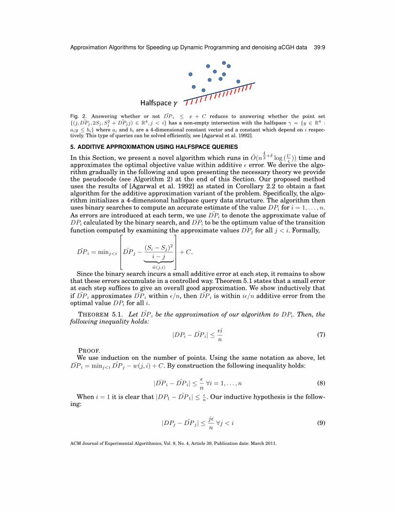
Fig. 2. Answering whether or not DP i ≤ x + C reduces to answering whether the point set{(j, ˜DPj , 2Sj , S

2j + ˜DPjj) ∈ R4, j < i} has a non-empty intersection with the halfspace γ = {y ∈ R4 :

aiy ≤ bi} where ai and bi are a 4-dimensional constant vector and a constant which depend on i respec-tively. This type of queries can be solved efficiently, see [Agarwal et al. 1992].

5. ADDITIVE APPROXIMATION USING HALFSPACE QUERIES

In this Section, we present a novel algorithm which runs in O(n43 +δ log (Uε )) time and

approximates the optimal objective value within additive ε error. We derive the algo-rithm gradually in the following and upon presenting the necessary theory we providethe pseudocode (see Algorithm 2) at the end of this Section. Our proposed methoduses the results of [Agarwal et al. 1992] as stated in Corollary 2.2 to obtain a fastalgorithm for the additive approximation variant of the problem. Specifically, the algo-rithm initializes a 4-dimensional halfspace query data structure. The algorithm thenuses binary searches to compute an accurate estimate of the value DPi for i = 1, . . . , n.As errors are introduced at each term, we use DPi to denote the approximate value ofDPi calculated by the binary search, and DPi to be the optimum value of the transitionfunction computed by examining the approximate values ˜DPj for all j < i. Formally,

DP i = minj<i

DP j − (Si − Sj)2

i− j︸︷︷︸w(j,i)

+ C.

Since the binary search incurs a small additive error at each step, it remains to showthat these errors accumulate in a controlled way. Theorem 5.1 states that a small errorat each step suffices to give an overall good approximation. We show inductively thatif DP i approximates DP i within ε/n, then DP i is within iε/n additive error from theoptimal value DPi for all i.

THEOREM 5.1. Let DP i be the approximation of our algorithm to DPi. Then, thefollowing inequality holds:

|DPi − DP i| ≤εi

n(7)

PROOF.We use induction on the number of points. Using the same notation as above, let

DP i = minj<i DP j − w(j, i) + C. By construction the following inequality holds:

|DP i − DP i| ≤ε

n∀i = 1, . . . , n (8)

When i = 1 it is clear that |DP1 − DP 1| ≤ εn . Our inductive hypothesis is the follow-

ing:

|DPj − DP j | ≤jε

n∀j < i (9)



It suffices to show that the following inequality holds:

|DPi − DP i| ≤(i− 1)ε

n(10)

since then by the triangular inequality we obtain:iε

n≥ |DPi − DP i|+ |DP i − DP i| ≥ |DPi − DP i|.

Let j∗, j be the optimum breakpoints for DPi and DP i respectively, j∗, j ≤ i− 1.

DPi = DPj∗ + w(j∗, i) + C

≤ DPj + w(j, i) + C

≤ DP j + w(j, i) + C +jε

n(by 9)

= DP i +jε

n

≤ DP i +(i− 1)ε

n

Similarly we obtain:

DP i = DP j + w(j, i) + C

≤ DP j∗ + w(j∗, i) + C

≤ DPj∗ + w(j∗, i) + C +j∗ε

n(by 9)

= DPi +j∗ε

n

≤ DPi +(i− 1)ε

n

Combining the above two inequalities, we obtain 10.

By substituting i = n in Theorem 5.1 we obtain the following corollary which provesthat DPn is within ε of DPn.

COROLLARY 5.2. Let DPn be the approximation of our algorithm to DPn. Then,

|DPn − DPn| ≤ ε. (11)

To use the analysis above in order to come up with an efficient algorithm we needto answer two questions: (a) How many binary search queries do we need in order toobtain the desired approximation? (b) How can we answer each such query efficiently?The answer to (a) is simple: as it can easily be seen, the value of the objective functionis upper bounded by U2n, where U = max {

√C, |P1|, . . . , |Pn|}. Therefore, O(log(U

2nε/n )) =

O(log (Uε )) iterations of binary search at each index i are sufficient to obtain the desiredapproximation. We reduce the answer to (b) to a well studied computational geometricproblem. Specifically, fix an index i, where 1 ≤ i ≤ n, and consider the general formof the binary search query DP i ≤ x + C, where x + C is the value on which we query.Note that we use the expression x+C for convenience, i.e., so that the constant C willbe simplified from both sides of the query. This query translates itself to the following



decision problem, see also Figure 2. Does there exist an index j, such that j < i andthe following inequality holds:

x ≥ ˜DPj −(Si − Sj)2

i− j⇒ xi+ S2

i ≥ (x, i, Si,−1)(j, ˜DPj , 2Sj , S2j + j ˜DPj)T ?

Hence, the binary search query has been reduced to answering a halfspace query.Specifically, the decision problem for any index i becomes whether the intersection ofthe point set POINTSi = {(j, ˜DPj , 2Sj , S2

j + ˜DPjj) ∈ R4, j < i} with a hyperplane isempty. By Corollary 2.2 [Agarwal et al. 1992], for a point set of size n, this can be donein O(n

13 +δ) per query and O(n

13 log n) amortized time per insertion of a point. Hence,

the optimal value of DPi can be found within an additive constant of ε/n using the

binary search in O(n13 log (Uε )) time.

Therefore, we can proceed from index 1 to n, find the approximately optimal valueof OPTi and insert a point corresponding to it into the query structure. We obtain analgorithm which runs in O(n

43 +δ log (Uε )) time, where δ is an arbitrarily small positive

constant. The pseudocode is given in Algorithm 2.

ALGORITHM 2: Approximation within additive ε using 4D halfspace queriesInitialize 4D halfspace query structure Qfor i = 1 to n do

low ← 0high← nU2

while high− low > ε/n dom← (low + high)/2/* This halfspace emptiness query is efficiently supported by Q */

flag ← (∃j such that xi+ S2i ≥ (x, i, Si,−1)(j, ˜DPj , 2Sj , S

2j + j ˜DPj)

T ) if flag thenhigh← m

elselow ← m

endendDP i ← (low + high)/2/* Point insertions are efficiently supported by Q */

Insert point (i, DP i, 2Si, S2i + DP ii) in Q

end

6. MULTISCALE MONGE DECOMPOSITIONIn this Section we present an algorithm which runs in O(n log n/ε) time to approxi-mate the optimal shifted objective value within a multiplicative factor of (1 + ε). Ouralgorithm is based on a new technique, which we consider of indepenent interest. Letw′(j, i) =

∑im=j+1(i − j)P 2

m − (Si − Sj)2. We can rewrite the weight function w as afunction of w′, namely as w(j, i) = w′(j, i)/(i− j) + C. The interested reader can easilycheck that we can express w′(j, i) as a sum of non-negative terms, i.e.,

w′(j, i) =∑

j+1≤m1<m2≤i

(Pm1 − Pm2)2.



Table I. Summary of proof of Lemma 6.1.

w′(i1, i4) + w′(i2, i3) w′(i1, i3) + w′(i2, i4)(S1, S1) 1 1(S2, S2) 2 2(S3, S3) 1 1(S1, S2) 1 1(S1, S3) 1 0(S2, S3) 1 1

Recall from Section 3 that the weight function w is not Monge. The next lemmashows that the weight function w′ is a Monge function.

LEMMA 6.1. The weight function w′(j, i) is Monge (concave), i.e., for any i1 < i2 <i3 < i4, the following holds:

w′(i1, i4) + w′(i2, i3) ≥ w′(i1, i3) + w′(i2, i4).

PROOF. Since each term in the summation is non-negative, it suffices to show thatany pair of indices, (m1,m2) is summed as many times on the left hand side as on theright hand side. If i2 + 1 ≤ m1 < m2 ≤ i3, each term is counted twice on each side.Otherwise, each term is counted once on the left hand side since i1 + 1 ≤ m1 < m2 ≤ i4and at most once on the right hand side since [i1 + 1, i3] ∩ [i2 + 1, i4] = [i2 + 1, i3].

The proof of Lemma 6.1 is summarized in Table I. Specifically, let Sj be the set ofindices {ij + 1, . . . , ij+1}, j = 1, 2, 3. Also, let (Sj , Sk) denote the set of indices (m1,m2)which appear in the summation such that m1 ∈ Sj ,m2 ∈ Sk. The two last columnsof Table I correspond to the left- and right-hand side of the Monge inequality (as inLemma 6.1) and contain the counts of appearances of each term.

Our approach is based on the following observations:

(1) Consider the weighted directed acyclic graph (DAG) on the vertex set V ={0, . . . , n} with edge set E = {(j, i) : j < i} and weight function w : E → R, i.e.,edge (j, i) has weight w(j, i). Solving the aCGH denoising problem reduces to find-ing a shortest path from vertex 0 to vertex n. If we perturb the edge weights withina factor of (1 + ε), as long as the weight of each edge is positive, then the optimalshortest path distance is also perturbed within a factor of at most (1 + ε).

(2) By Lemma 6.1 we obtain that the weight function is not Monge essentially becauseof the i− j term in the denominator.

(3) Our goal is to approximate w by a Monge function w′ such that c1w′ ≤ w ≤ c2w′

where c1, c2 should be known constants.

In the following we elaborate on the latter goal. Fix an index i and note that theoptimal breakpoint for that index is some index j ∈ {1, . . . , i − 1}. We will “bucketize”the range of index j into m = O(log1+ε (i)) = O(log n/ε) buckets such that the k-thbucket, k = 1, . . . ,m, is defined by the set of indices j which satisfy

lk = i− (1 + ε)k ≤ j ≤ i− (1 + ε)k−1 = rk.

This choice of bucketization is based on the first two observations which guide ourapproach. Specifically, it is easy to check that (1 + ε)k−1 ≤ i− j ≤ (1 + ε)k. This results,for any given i, to approximating i−j by a constant for each possible bucket, leading toO(log n/ε) different Monge functions (one per bucket) while incurring a multiplicativeerror of at most (1 + ε). However, there exists a subtle point, as also Figure 3 indicates.We need to make sure that each of the Monge functions is appropriatelly defined sothat when we consider the k-th Monge subproblem, the optimal breakpoint jk should



satisfy jk ∈ [lk, rk]. Having achieved that (see Lemma 6.2) we can solve efficiently therecurrence. Specifically, OPTi is computed as follows:

OPTi = minj<i

[OPTj +

w′(i, j)i− j

]+ C

= mink

[min

j∈[lk,rk]OPTj +

w′(i, j)i− j

]+ C

≈ mink

[min

j∈[lk,rk]OPTj +

w′(i, j)(1 + ε)k−1

]+ C

= mink

[min

j∈[lk,rk]OPTj +

w′(i, j)ck

]+ C.

The following is one of the possible ways to define the m Monge weight functions. Inwhat follows, λ is a sufficiently large positive constant.

wk(j, i) =

2n−i+jλ i− j < ck = (1 + ε)k−1

2i−jλ i− j > (1 + ε)ck = (1 + ε)kw′(j, i)/ck otherwise

(12)

LEMMA 6.2. Given any vector P , it is possible to pick λ such that wk is Monge forall k ≥ 1. That is, for any 4-tuple i1 < i2 < i3 < i4, wk(i1, i4) + wk(i2, i3) ≥ wk(i1, i3) +wk(i2, i4).

PROOF. Since w′(j, i) =∑j+1≤m1<m2≤i(Pm1 − Pm2)2 ≤ (2K)2n2 where K =

max1≤i≤n |Pi|, we can pick λ such that wk(j, i) ≥ w′(j, i). The rest of the proof is case-work based on the lengths of the intervals i3− i1, i4− i2, and how they compare with ckand (1 + ε)ck. There are 12 such cases in total. We may assume i3− i1 ≤ i4− i2 withoutloss of generality, leaving thus 6 cases to be considered.If ck ≤ i3 − i1, i4 − i2 ≤ (1 + ε)ck, then:

wk(i1, i3) + wk(i2, i4) = (1/ck)(w′(i1, i3) + w′(i2, i4))

≤ (1/ck)(w′(i1, i4) + w′(i2, i3)) (by Lemma 6.1)≤ wk(i1, i4) + wk(i2, i3).

If i3 − i1 < ck and i4 − i2 ≤ (1 + ε)ck. Then as i2 > i1, i3 − i2 ≤ i3 − i1 − 1 and we have:

wk(i2, i3) = 2n−i3+i2λ

≥ 2 · 2n−i3−i1λ≥ wk(i1, i3) + wk(i2, i4)

The cases of ck ≤ i3 − i1 and ck(1 + ε) < i4 − i2 can be done similarly. Note that thecases of i3 − i1, i4 − i2 < ck and (1 + ε)ck < i3 − i1, i4 − i2 are also covered by these.

The only case that remain is i3− i1 < ck and (1+ε)ck < i4− i2. Since i3− i2 < i3− i1 <ck, we have:

wk(i2, i3) = 2n−i3+i2λ

> 2n−i4+i2λ

= wk(i2, i4)



Fig. 3. Solving the k-th Monge problem, k = 1, . . . ,m = O(log1+ε (i)), for a fixed index i. The k-th intervalis the set of indices {j : lk ≤ j ≤ rk, lk = i− (1+ ε)k, rk = i− (1+ ε)k−1}. Ideally, we wish to define a Mongefunction w′k whose maximum inside the k-th interval (red color) is smaller than the minimum outside thatinterval (green color). This ensures that the optimal breakpoint for the k-th Monge subproblem lies insidethe red interval.

Similarly wk(i1, i4) = 2i4−i1λ > 2i3−i1λ = wk(i1, i3). Adding them gives the desiredresult.

The pseudocode is shown in Algorithm 3. The algorithm computes the OPT valuesonline time based on the above analysis. In order to solve each Monge sub-problem ourmethod calls the routine of Theorem 2.3. For each index i, we compute OPTi by takingthe best value over queries to all k of the Monge query structures, then we update allthe structures with this value. Note that storing values of the form 2kλ using only theirexponent k suffices for comparison, so introducing wk(j, i) doesn’t result in any changein runtime. By Theorem 2.3, for each Qk, finding minj<iQk.aj +wk(j, i) over all i takesO(n) time. Hence, the total runtime is O(n log n/ε).

ALGORITHM 3: Approximation within a factor of ε using Monge function search/* The weight function wk(j, i) is Monge. Specifically,

wk(j, i) = C +“Pi

m=j+1(i− j)P2m −

(Si−Sj)2

(1+ε)k

”for all j which satisfy

(1 + ε)k−1 ≤ i− j ≤ (1 + ε)k. */Maintain m = log n/ log (1 + ε) Monge function search data structures Q1, . . . , Qm where Qkcorresponds to the Monge function wk(j, i).OPT0 ← 0/* Recursion basis */for k = 1 to m do

Qk.a0 ← 0endfor i = 1 to n do

OPTi ←∞for k = 1 to m do

/* Let a(k)j denote Qk.aj, i.e., the value aj of the k-th data structure Qk

*/localmink ← minj<i a

(k)j + wk(j, i)

OPTi ← min{OPTi, localmink + C}end

endfor k = 1 to m do

Qk.ai ← OPTiend



Table II. Datasets, papers and the URLs where the datasets can be downloaded. �and � denote which datasets are synthetic and real respectively.

Dataset Availability� Lai et al. [Lai et al. 2005]

http://compbio.med.harvard.edu/� Willenbrock et al. [Willenbrock and Fridlyand 2005]

http://www.cbs.dtu.dk/~hanni/aCGH/� Coriell Cell lines [Snijders et al. 2001]

http://www.nature.com/ng/journal/v29/n3/� Berkeley Breast Cancer [Neve et al. 2006]

http://icbp.lbl.gov/breastcancer/

7. VALIDATION OF OUR MODELIn this Section we validate our model using the exact algorithm, see Section 3. InSection 7.1 we describe the datasets and the experimental setup. In Section 7.2 weshow the findings of our method together with a detailed biological analysis.

7.1. Experimental Setup and DatasetsOur code is implemented in MATLAB2. The experiments run in a 4GB RAM, 2.4GHzIntel(R) Core(TM)2 Duo CPU, Windows Vista machine. Our methods were comparedto existing MATLAB implementations of the CBS algorithm, available via the Bioin-formatics toolbox, and the CGHSEG algorithm [Picard et al. 2005], courteously pro-vided to us by Franc Picard. CGHSEG was run using heteroscedastic model un-der the Lavielle criterion [Lavielle 2005]. Additional tests using the homoscedasticmodel showed substantially worse performance and are omitted here. All methodswere compared using previously developed benchmark datasets, shown in Table II.Follow-up analysis of detected regions was conducted by manually searching for signif-icant genes in the Genes-to-Systems Breast Cancer Database http://www.itb.cnr.it/breastcancer [Viti et al. 2009] and validating their positions with the UCSC GenomeBrowser http://genome.ucsc.edu/. The Atlas of Genetics and Cytogenetics in Oncol-ogy and Haematology http://atlasgeneticsoncology.org/ was also used to validatethe significance of reported cancer-associated genes. It is worth pointing out that sinceaCGH data are typically given in the log scale, we first exponentiate the points, thenfit the constant segment by taking the average of the exponentiated values from thehypothesized segment, and then return to the log domain by taking the logarithm ofthat constant value. Observe that one can fit a constant segment by averaging thelog values using Jensen’s inequality, but we favor an approach more consistent withthe prior work, which typically models the data assuming i.i.d. Gaussian noise in thelinear domain.

How to pick C?. The performance of our algorithm depends on the value of the pa-rameter C, which determines how much each segment “costs.” Clearly, there is a trade-off between larger and smaller values: excessively large C will lead the algorithm tooutput a single segment while excessively small C will result in each point being fit asits own segment. We pick our parameter C using data published in [Willenbrock andFridlyand 2005]. The data was generated by modeling real aCGH data, thus capturingtheir nature better than other simplified synthetic data and also making them a goodtraining dataset for our model. We used this dataset to generate a Receiver OperatingCharacteristic (ROC) curve using values for C ranging from 0 to 4 with increment 0.01using one of the four datasets in [Willenbrock and Fridlyand 2005] (“above 20”). The

2Code available at URL http://www.math.cmu.edu/~ctsourak/CGHTRIMMER.zip. Faster C code is also avail-able, but since the competitors were implemented in MATLAB, all the results in this Section refer to ourMATLAB implementation.



Fig. 4. ROC curve of CGHTRIMMER as a function of C on data from [Willenbrock and Fridlyand 2005]. Thered arrow indicates the point (0.91 and 0.98 recall and precision respectively) corresponding to C=0.2, thevalue used in all subsequent results.

resulting curve is shown in Figure 4. Then, we selected C = 0.2, which achieves highprecision/specificity (0.98) and high recall/sensitivity (0.91). All subsequent results re-ported were obtained by setting C equal to 0.2.

7.2. Experimental Results and Biological AnalysisWe show the results on synthetic data in Section 7.2.1, on real data where the groundtruth is available to us in Section 7.2.2 and on breast cancer cell lines with no groundtruth in Section 7.2.3.

7.2.1. Synthetic Data. We use the synthetic data published in [Lai et al. 2005]. The dataconsist of five aberrations of increasing widths of 2, 5, 10, 20 and 40 probes, respec-tively, with Gaussian noise N(0,0.252). Figure 5 shows the performance of CGHTRIM-MER, CBS, and CGHSEG. Both CGHTRIMMER and CGHSEG correctly detect all aber-rations, while CBS misses the first, smallest region. The running time for CGHTRIM-MER is 0.007 sec, compared to 1.23 sec for CGHSEG and 60 sec for CBS.

7.2.2. Coriell Cell Lines. The first real dataset we use to evaluate our method is theCoriell cell line BAC array CGH data [Snijders et al. 2001], which is widely considereda “gold standard” dataset. The dataset is derived from 15 fibroblast cell lines using thenormalized average of log2 fluorescence relative to a diploid reference. To call gains orlosses of inferred segments, we assign to each segment the mean intensity of its probesand then apply a simple threshold test to determine if the mean is abnormal. We follow[Bejjani et al. 2005] in favoring ±0.3 out of the wide variety of thresholds that havebeen used [Ng et al. 2006].

Table III summarizes the performance of CGHTRIMMER, CBS and CGHSEG rela-tive to previously annotated gains and losses in the Corielle dataset. The table showsnotably better performance for CGHTRIMMER compared to either alternative method.CGHTRIMMER finds 22 of 23 expected segments with one false positive. CBS finds20 of 23 expected segments with one false positive. CGHSEG finds 22 of 23 expectedsegments with seven false positives. CGHTRIMMER thus achieves the same recall as



(a) CGHTRIMMER (b) CBS

(c) CGHSEG

Fig. 5. Performance of CGHTRIMMER, CBS, and CGHSEG on denoising synthetic aCGH data from [Laiet al. 2005]. CGHTRIMMER and CGHSEG exhibit excellent precision and recall whereas CBS misses twoconsecutive genomic positions with DNA copy number equal to 3.

CGHSEG while outperforming it in precision and the same precision as CBS while out-performing it in recall. In cell line GM03563, CBS fails to detect a region of two pointswhich have undergone a loss along chromosome 9, in accordance with the results ob-tained using the Lai et al. [Lai et al. 2005] synthetic data. In cell line GM03134, CGH-SEG makes a false positive along chromosome 1 which both CGHTRIMMER and CBSavoid. In cell line GM01535, CGHSEG makes a false positive along chromosome 8 andCBS misses the aberration along chromosome 12. CGHTRIMMER, however, performsideally on this cell line. In cell line GM02948, CGHTRIMMER makes a false positivealong chromosome 7, finding a one-point segment in 7q21.3d at genomic position 97000whose value is equal to 0.732726. All other methods also make false positive errors onthis cell line. In GM7081, all three methods fail to find an annotated aberration onchromosome 15. In addition, CGHSEG finds a false positive on chrosome 11.

CGHTRIMMER also substantially outperforms the comparative methods in run time,requiring 5.78 sec for the full data set versus 8.15 min for CGHSEG (an 84.6-foldspeedup) and 47.7 min for CBS (a 495-fold speedup).

7.2.3. Breast Cancer Cell Lines. To illustrate further the performance of CGHTRIMMERand compare it to CBS and CGHSEG, we applied it to the Berkeley Breast Cancercell line database [Neve et al. 2006]. The dataset consists of 53 breast cancer cell linesthat capture most of the recurrent genomic and transcriptional characteristics of 145primary breast cancer cases. We do not have an accepted “answer key” for this data



Table III. Results from applying CGHTRIMMER, CBS, and CGH-SEG to 15 cell lines. Rows with listed chromosome numbers (e.g.,GM03563/3) corresponded to known gains or losses and are anno-tated with a check mark if the expected gain or loss was detected ora “No” if it was not. Additional rows list chromosomes on which seg-ments not annotated in the benchmark were detected; we presumethese to be false positives.

Cell Line/Chromosome CGHTRIMMER CBS CGHSEGGM03563/3 X X XGM03563/9 X No X

GM03563/False - - -GM00143/18 X X X

GM00143/False - - -GM05296/10 X X XGM05296/11 X X X

GM05296/False - - 4,8GM07408/20 X X X

GM07408/False - - -GM01750/9 X X X

GM01750/14 X X XGM01750/False - - -

GM03134/8 X X XGM03134/False - - 1

GM13330/1 X X XGM13330/4 X X X

GM13330/False - - -GM03576/2 X X X

GM03576/21 X X XGM03576/False - - -

GM01535/5 X X XGM01535/12 X No X

GM01535/False - - 8GM07081/7 X X X

GM07081/15 No No NoGM07081/False - - 11

GM02948/13 X X XGM02948/False 7 1 2

GM04435/16 X X XGM04435/21 X X X

GM04435/False - - 8,17GM10315/22 X X X

GM10315/False - - -GM13031/17 X X X

GM13031/False - - -GM01524/6 X X X

GM01524/False - - -

set, but it provides a more extensive basis for detailed comparison of differences inperformance of the methods on common data sets, as well as an opportunity for noveldiscovery. While we have applied the methods to all chromosomes in all cell lines, spacelimitations prevent us from presenting the full results here. The interested reader canreproduce all the results including the ones not presented here3. We therefore arbi-trarily selected three of the 53 cell lines and selected three chromosomes per cell linethat we believed would best illustrate the comparative performance of the methods.The Genes-to-Systems Breast Cancer Database 4 [Viti et al. 2009] was used to identify

3http://www.math.cmu.edu/~ctsourak/DPaCGHsupp.html4http://www.itb.cnr.it/breastcancer



(a) (b) (c)

(d) (e) (f)

(g) (h) (i)

CGHTRIMMER CBS CGHSEG

Fig. 6. Visualization of the segmentation output of CGHTRIMMER, CBS, and CGHSEG for the cell lineBT474 on chromosomes 1 (a,b,c), 5 (d,e,f), and 17 (g,h,i). (a,d,g) CGHTRIMMER output. (b,e,h) CBS output.(c,f,i) CGHSEG output. Segments exceeding the ± 0.3 threshold [Bejjani et al. 2005] are highlighted.

known breast cancer markers in regions predicted to be gained or lost by at least oneof the methods. We used the UCSC Genome Browser 5 to verify the placement of genes.

We note that CGHTRIMMER again had a substantial advantage in run time. For thefull data set, CGHTRIMMER required 22.76 sec, compared to 23.3 min for CGHSEG (a61.5-fold increase), and 4.95 hrs for CBS (a 783-fold increase).

Cell Line BT474:. Figure 6 shows the performance of each method on the BT474cell line. The three methods report different results for chromosome 1, as shown in Fig-ures 6(a,b,c), with all three detecting amplification in the q-arm but differing in the de-tail of resolution. CGHTRIMMER is the only method that detects region 1q31.2-1q31.3as aberrant. This region hosts gene NEK7, a candidate oncogene [Kimura and Okano2001] and gene KIF14, a predictor of grade and outcome in breast cancer [Corson et al.2005]. CGHTRIMMER and CBS annotate the region 1q23.3-1q24.3 as amplified. Thisregion hosts several genes previously implicated in breast cancer [Viti et al. 2009],such as CREG1 (1q24), POU2F1 (1q22-23), RCSD1 (1q22-q24), and BLZF1 (1q24). Fi-nally, CGHTRIMMER alone reports independent amplification of the gene CHRM3, amarker of metastasis in breast cancer patients [Viti et al. 2009].

For chromosome 5 (Figures 6(d,e,f)), the behavior of the three methods is al-most identical. All methods report amplification of a region known to contain many

5http://genome.ucsc.edu/



(a) (b) (c)

(d) (e) (f)

(g) (h) (i)


Fig. 7. Visualization of the segmentation output of CGHTRIMMER, CBS, and CGHSEG for the cell lineHS578T on chromosomes 3 (a,b,c), 11 (d,e,f), and 17 (g,h,i). (a,d,g) CGHTRIMMER output. (b,e,h) CBS output.(c,f,i) CGHSEG output. Segments exceeding the ± 0.3 threshold [Bejjani et al. 2005] are highlighted.

breast cancer markers, including MRPL36 (5p33), ADAMTS16 (5p15.32), POLS(5p15.31), ADCY2 (5p15.31), CCT5 (5p15.2), TAS2R1 (5p15.31), ROPN1L (5p15.2),DAP (5p15.2), ANKH (5p15.2), FBXL7 (5p15.1), BASP1 (5p15.1), CDH18 (5p14.3),CDH12 (5p14.3), CDH10 (5p14.2 - 5p14.1), CDH9 (5p14.1) PDZD2 (5p13.3), GOLPH3(5p13.3), MTMR12 (5p13.3), ADAMTS12 (5p13.3 - 5p13.2), SLC45A2 (5p13.2), TARS(5p13.3), RAD1 (5p13.2), AGXT2 (5p13.2), SKP2 (5p13.2), NIPBL (5p13.2), NUP155(5p13.2), KRT18P31 (5p13.2), LIFR (5p13.1) and GDNF (5p13.2) [Viti et al. 2009]. Theonly difference in the assignments is that CBS fits one more probe to this amplifiedsegment.

Finally, for chromosome 17 (Figures 6(g,h,i)), like chromosome 1, all methods detectamplification but CGHTRIMMER predicts a finer breakdown of the amplified regioninto independently amplified segments. All three methods detect amplification of aregion which includes the major breast cancer biomarkers HER2 (17q21.1) and BRCA1(17q21) as also the additional markers MSI2 (17q23.2) and TRIM37 (17q23.2) [Vitiet al. 2009]. While the more discontiguous picture produced by CGHTRIMMER mayappear to be a less parsimonious explanation of the data, a complex combination offine-scale gains and losses in 17q is in fact well supported by the literature [Orsettiet al. 2004].

Cell Line HS578T:. Figure 7 compares the methods on cell line HS578T for chro-mosomes 3, 11 and 17. Chromosome 3 (Figures 7(a,b,c)) shows identical prediction



(a) (b) (c)

(d) (e) (f)

(g) (h) (i)


Fig. 8. Visualization of the segmentation output of CGHTRIMMER, CBS, and CGHSEG for the cell lineT47D on chromosomes 1 (a,b,c), 11 (d,e,f), and 20 (g,h,i). (a,d,g) CGHTRIMMER output. (b,e,h) CBS output.(c,f,i) CGHSEG output. Segments exceeding the ± 0.3 threshold [Bejjani et al. 2005] are highlighted.

of an amplification of 3q24-3qter for all three methods. This region includes the keybreast cancer markers PIK3CA (3q26.32) [Lee et al. 2005], and additional breast-cancer-associated genes TIG1 (3q25.32), MME (3q25.2), TNFSF10 (3q26), MUC4(3q29), TFRC (3q29), DLG1 (3q29) [Viti et al. 2009]. CGHTRIMMER and CGHSEG alsomake identical predictions of normal copy number in the p-arm, while CBS reports anadditional loss between 3p21 and 3p14.3. We are unaware of any known gain or lossin this region associated with breast cancer.

For chromosome 11 (Figures 7(d,e,f)), the methods again present an identical pictureof loss at the q-terminus (11q24.2-11qter) but detect amplifications of the p-arm at dif-ferent levels of resolution. CGHTRIMMER and CBS detect gain in the region 11p15.5,which is the site of the HRAS breast cancer metastasis marker [Viti et al. 2009]. Incontrast to CBS, CGHTRIMMER detects an adjacent loss region. While we have no di-rect evidence this loss is a true finding, the region of predicted loss does contain EIF3F(11p15.4), identified as a possible tumor suppressor whose expression is decreased inmost pancreatic cancers and melanomas [Viti et al. 2009]. Thus, we conjecture thatEIF3F is a tumor suppressor in breast cancer.

On chromosome 17 (Figures 7(g,h,i)), the three methods behave similarly, with allthree predicting amplification of the p-arm. CBS places one more marker in the am-plified region causing it to cross the centromere while CGHSEG breaks the amplifiedregion into three segments by predicting additional amplification at a single marker.



(a) (b) (c)

(d) (e) (f)

(g) (h) (i)


Fig. 9. Visualization of the segmentation output of CGHTRIMMER, CBS, and CGHSEGfor the cell lineMCF10A on chromosomes 1 (a,b,c), 8 (d,e,f), and 20 (g,h,i). (a,d,g) CGHTRIMMER output. (b,e,h) CBS output.(c,f,i) CGHSEG output. Segments exceeding the ± 0.3 threshold [Bejjani et al. 2005] are highlighted.

Cell Line T47D:. Figure 8 compares the methods on chromosomes 1, 8, and 20 ofthe cell line T47D. On chromosome 1 (Figure 8(a,b,c)), all three methods detect lossof the p-arm and a predominant amplification of the q-arm. CBS infers a presumablyspurious extension of the p-arm loss across the centromere into the q-arm, while theother methods do not. The main differences between the three methods appear onthe q-arm of chromosome 1. CGHTRIMMER and CGHSEG detect a small region ofgain proximal to the centromere at 1q21.1-1q21.2, followed by a short region of lossspanning 1q21.3-1q22. CBS merges these into a single longer region of normal copynumber. The existence of a small region of loss at this location in breast cancers issupported by prior literature [Chunder et al. 2003].

The three methods provide comparable segmentations of chromosome 11 (Fig-ure 8(d,e,f)). All predict loss near the p-terminus, a long segment of amplificationstretching across much of the p- and q-arms, and additional amplification near theq-terminus. CGHTRIMMER, however, breaks this q-terminal amplification into severalsub-segments at different levels of amplification while CBS and CGHSEG both fit asingle segment to that region. We have no empirical basis to determine which segmen-tation is correct here. CGHTRIMMER does appear to provide a spurious break in thelong amplified segment that is not predicted by the others.

Finally, along chromosome 20 (Figure 8(g,h,i)), the output of the methods is similar,with all three methods suggesting that the q-arm has an aberrant copy number, anobservation consistent with prior studies [Hodgson et al. 2003]. The only exception is



again that CBS fits one point more than the other two methods along the first segment,causing a likely spurious extension of the p-arm’s normal copy number into the q-arm.

Cell Line MCF10A. Figure 9 shows the output of each of the three methods on chro-mosomes 1, 8, and 20 of the cell line MCF10A. On this cell line, the methods all yieldsimilar predictions although from slightly different segmentations. All three shownearly identical behavior on chromosome 1 (Figure 9(a,b,c)), with normal copy num-ber on the p-arm and at least two regions of independent amplification of the q-arm.Specifically, the regions noted as gain regions host significant genes such as PDE4DIPa gene associated with breast metastatic to bone (1q22), ECM1 (1q21.2), ARNT (1q21),MLLT11 (1q21), S100A10 (1q21.3), S100A13 (1q21.3), TPM3 (1q25) which also plays arole in breast cancer metastasis, SHC1 (1q21.3) and CKS1B (1q21.3). CBS provides aslightly different segmentation of the q-arm near the centromere, suggesting that thenon-amplified region spans the centromere and that a region of lower amplificationexists near the centromere. On chromosome 8 (Figure 9(d,e,f)) the three algorithmslead to identical copy number predictions after thresholding, although CBS inserts anadditional breakpoint at 8q21.3 and a short additional segment at 8q22.2 that do notcorrespond to copy number changes. All three show significant amplification acrosschromosome 20 (Figure 9(g,h,i)), although in this case CGHSEG distinguishes an ad-ditional segment from 20q11.22-20q11.23 that is near the amplification threshold. Itis worth mentioning that chromosome 20 hosts significant breast cancer related genessuch as CYP24 and ZNF217.

8. CONCLUSIONSIn this paper, we present a new formulation for the problem of denoising aCGH data.Our formulation has already proved to be valuable in numerous settings [Ding andShah 2010]. We show a basic exact dynamic programming algorithm which runs inO(n2) time and performs excellently on both synthetic and real data. More interest-ingly from a theoretical perspective, we develop two techniques for performing approx-imate dynamic programming in both the additive and the multiplicative norm. Ourfirst algorithm reduces the optimization problem into a well studied geometric prob-lem, namely halfspace emptiness queries. The second technique carefully breaks theproblem into a small number of Monge subproblems, which are solved efficiently usingexisting techniques. Our results strongly indicate that the O(n2) algorithm, which is— to the best of our knowledge — the fastest exact algorithm, is not tight. There isinherent structure in the optimization problem. Lemma 8.1 is such an example.

(a) One fitted segment

(b) Five fitted segments

Fig. 10. Lemma 8.1: if |Pi1 − Pi2 | > 2√

2C then Segmentation (b) which consists of five segments (two ofwhich are single points) is superior to Segmentation (a) which consists of a single segment.



LEMMA 8.1. If |Pi1 − Pi2 | > 2√

2C, then in the optimal solution of the dynamic pro-gramming using L2 norm, i1 and i2 are in different segments.

PROOF. The proof is by contradiction, see also Figure 10. Suppose the optimal so-lution has a segment [i, j] where i ≤ i1 < i2 ≤ j, and its optimal x value is x∗. Thenconsider splitting it into 5 intervals [i, i1 − 1], [i1, i1], [i1 + 1, i2 − 1], [i2, i2], [i2 + 1, r].We let x = x∗ be the fitted value to the three intervals not containing i1 and i2. Also,as |Pi1 − Pi2 | > 2

√2C, (Pi1 − x)2 + (Pi2 − x)2 > 2

√2C

2= 4C. So by letting x = Pi1 in

[i1, i1] and x = Pi2 in [i2, i2], the total decreases by more than 4C. This is more than theadded penalty of having 4 more segments, a contradiction with the optimality of thesegmentation.

Uncovering and taking advantage of the inherent structure in a principled wayshould result in a faster exact algorithm. This is an interesting research directionwhich we leave as future work. Another research direction is to find more applications(e.g., histogram construction [Guha et al. 2006]) to which our methods are applicable.

ACKNOWLEDGMENTS

The authors would like to thank Frank Picard for making his MATLAB code available to us. We would liketo thank Pawel Gawrychowski for pointing us reference [Agarwal et al. 1992] and Dimitris Achlioptas andYuan Zhou for helpful discussions on optimization techniques. We would also like to thank the reviewers fortheir valuable comments.

REFERENCESAGARWAL, P. K., EPPSTEIN, D., AND MATOUSEK, J. 1992. Dynamic half-space reporting, geometric opti-

mization, and minimum spanning trees. In Proceedings of the 33rd Annual Symposium on Foundationsof Computer Science. IEEE Computer Society, Washington, DC, USA, 80–89.

AGARWAL, P. K. AND ERICKSON, J. 1999. Geometric Range Searching and Its Relatives.AGGARWAL, A., HANSEN, M., AND LEIGHTON, T. 1990. Solving query-retrieval problems by compacting

voronoi diagrams. In Proceedings of the twenty-second annual ACM symposium on Theory of computing.STOC ’90. ACM, New York, NY, USA, 331–340.

AGGARWAL, A., KLAWE, M., MORAN, S., SHOR, P., AND WILBER, R. 1986. Geometric applications of a ma-trix searching algorithm. In Proceedings of the second annual symposium on Computational geometry.SCG ’86. ACM, New York, NY, USA, 285–292.

ALBERTSON, D. AND PINKEL, D. 2003. Genomic microarrays in human genetic disease and cancer. HumanMolecular Genetics 12, 145–152.

BARRY, D. AND HARTIGAN, J. 1993. A bayesian analysis for change point problems. Journal of the AmericanStatistical Association 88, 421, 309–319.

BEIN, W., GOLIN, M., LARMORE, L., AND ZHANG, Y. 2009. The knuth-yao quadrangle-inequality speedupis a consequence of total monotonicity. ACM Trans. Algorithms 6, 1–22.

BEJJANI, B., SALEKI, R., BALLIF, B., ROREM, E., SUNDIN, K., THEISEN, A., KASHORK, C., AND SHAFFER,L. 2005. Use of targeted array-based cgh for the clinical diagnosis of chromosomal imbalance: is lessmore? American Journal of Medical Genetics A, 259–67.

BELLMAN, R. 2003. Dynamic Programming. Dover Publications.BERTSEKAS, D. 2000. Dynamic Programming and Optimal Control. Athena Scientific.BIGNELL, G., HUANG, J., GRESHOCK, J., WATT, S., BUTLER, A., WEST, S., GRIGOROVA, M., JONES, K.,

WEI, W., STRATTON, M., FUTREAL, A., WEBER, B., SHAPERO, M., AND WOOSTER, R. 2004. High-resolution analysis of dna copy number using oligonucleotide microarrays. Genome Research, 287–295.

BURKARD, R. E., KLINZ, B., AND RUDIGER, R. 1996. Perspectives of monge properties in optimization.Discrete Appl. Math. 70, 95–161.

BUTLER, M., MEANEY, F., AND PALMER, C. 1986. Clinical and cytogenetic survey of 39 individuals withprader-labhart-willi syndrome. American Journal of Medical Genetics 23, 793–809.

CHAZELLE, B., GUIBAS, L., AND LEE, D. T. 1985. The power of geometric duality. BIT 25, 76–90.



CHAZELLE, B. AND PREPARATA, F. 1985. Halfspace range search: an algorithmic application of k-sets. InProceedings of the first annual symposium on Computational geometry. SCG ’85. ACM, New York, NY,USA, 107–115.

CHUNDER, N., MANDAL, S., BASU, D., ROY, A., ROYCHOUDHURY, S., AND PANDA, C. K. 2003. Deletionmapping of chromosome 1 in early onset and late onset breast tumors–a comparative study in easternindia. Pathol Res Pract 199, 313–321.

CLARKSON, K. L. AND SHOR., P. W. 1989. Applications of random sampling in computational geometry, ii.Discrete Comput. Geom. 4, 387–421.

CORSON, T., HUANG, A., TSAO, M., AND GALLIE, B. 2005. Kif14 is a candidate oncogene in the 1q minimalregion of genomic gain in multiple cancers. Oncogene 24, 47414753.

DESPER, R., JIANG, F., KALLIONIEMI, O.-P., MOCH, H., PAPADIMITRIOU, C. H., AND SCHAFFER, A. A.1999. Inferring tree models for oncogenesis from comparative genome hybridization data. Journal ofComputational Biology 6, 1, 37–52.

DESPER, R., JIANG, F., KALLIONIEMI, O.-P., MOCH, H., PAPADIMITRIOU, C. H., AND SCHAFFER, A. A.2000. Distance-based reconstruction of tree models for oncogenesis. Journal of Computational Biol-ogy 7, 6, 789–803.

DING, J. AND SHAH, S. P. 2010. Robust hidden semi-markov modeling of array cgh data. In IEEE Interna-tional Conference on Bioinformatics & Biomedicine. 603–608.

EILERS, P. H. AND DE MENEZES, R. X. 2005. Quantile smoothing of array cgh data. Bioinformatics 21, 7,1146–1153.

EPPSTEIN, D., GALIL, Z., AND GIANCARLO, R. 1988. Speeding up dynamic programming. In Proceedings ofthe 29th Annual Symposium on Foundations of Computer Science. IEEE Computer Society, Washington,DC, USA, 488–496.

EPPSTEIN, D., GALIL, Z., GIANCARLO, R., AND ITALIANO, G. 1992a. Sparse dynamic programming i: linearcost functions. J. ACM 39, 519–545.

EPPSTEIN, D., GALIL, Z., GIANCARLO, R., AND ITALIANO, G. 1992b. Sparse dynamic programming ii:convex and concave cost functions. J. ACM 39, 546–567.

FRIDLYAND, J., SNIJDERS, A. M., PINKEL, D., ALBERTSON, D. G., AND JAIN, A. N. 2004. Hidden markovmodels approach to the analysis of array cgh data. J. Multivar. Anal. 90, 1, 132–153.

GILBERT, E. AND MOORE, E. 1959. Variable-length binary encodings. Bell System Tech. 38, 933–966.GUHA, S., KOUDAS, N., AND SHIM, K. 2006. Approximation and streaming algorithms for histogram con-

struction problems. ACM Trans. Database Syst. 31, 396–438.GUHA, S., LI, Y., AND NEUBERG, D. 2006. Bayesian hidden markov modeling of array cgh data. Harvard

University, Paper 24.HIRSCHBERG, D. 1975. A linear space algorithm for computing maximal common subsequences. Commun.

ACM 18, 341–343.HODGSON, J., CHIN, K., COLLINS, C., AND GRAY, J. 2003. Genome amplification of chromosome 20 in breast

cancer. Breast Cancer Res Treat..HSU, L., SELF, S., GROVE, D., WANG, K., DELROW, J., LOO, L., AND PORTER, P. 2005. Denoising array

based comparative genomic hybridization data using wavelets. Biostatistics 6, 211–226.HUANG, T., WU, B., LIZARDI, P., AND ZHAO, H. 2005. Detection of DNA copy number alterations using

penalized least squares regression. Bioinformatics 21, 20, 3811–3817.HUPE, P., STRANSKY, N., THIERY, J.-P., RADVANYI, F., AND BARILLOT, E. 2004. Analysis of array cgh data:

from signal ratio to gain and loss of dna regions. Bioinformatics 20, 18, 3413–3422.JAGADISH, H. V., KOUDAS, N., MUTHUKRISHNAN, S., POOSALA, V., SEVCIK, K. C., AND TORSTEN, S.

1998. Optimal histograms with quality guarantees. In Proceedings of the 24rd International Conferenceon Very Large Data Bases. VLDB ’98. Morgan Kaufmann Publishers Inc., San Francisco, CA, USA,275–286.

JONG, K., MARCHIORI, E., MEIJER, G., VAN DER VAART, A., AND YLSTRA, B. 2004. Breakpoint identifica-tion and smoothing of array comparative genomic hybridization data. Bioinformatics 20, 18, 3636–3637.

KALLIONIEMI, A., KALLIONIEMI, O., SUDAR, D., RUTOVITZ, D., GRAY, J., WALDMAN, F., AND PINKEL,D. 1992. Comparative genomic hybridization for molecular cytogenetic analysis of solid tumors. Sci-ence 258, 5083, 818–821.

KIMURA, M. AND OKANO, Y. 2001. Identification and assignment of the human nima-related protein kinase7 gene (nek7) to human chromosome 1q31.3. Cytogenet. Cell Genet..

KLAWE, M. AND KLEITMAN, D. 1990. An almost linear time algorithm for generalized matrix searching.SIAM J. Discret. Math. 3, 81–97.



KNUTH, D. E. 1971. Optimum binary search trees. Acta Inf. 1, 14–25.KNUTH, D. E. 1981. Seminumerical Algorithms. Addison-Wesley.LAI, W. R., JOHNSON, M. D., KUCHERLAPATI, R., AND PARK, P. J. 2005. Comparative analysis of algo-

rithms for identifying amplifications and deletions in array cgh data. Bioinformatics 21, 19, 3763–3770.LARMORE, L. L. AND SCHIEBER, B. 1991. On-line dynamic programming with applications to the prediction

of rna secondary structure. J. Algorithms 12, 3, 490–515.LAVIELLE, M. 2005. Using penalized contrasts for the change-point problem. Signal Processing 85, 8, 1501–

1510.LEE, J. W., SOUNG, Y. H., KIM, S. Y., LEE, H. W., PARK, W. S., NAM, S. W., KIM, S. H., LEE, J. Y., YOO,

N. J., , AND LEE, S. H. 2005. Pik3ca gene is frequently mutated in breast carcinomas and hepatocellularcarcinomas. Oncogene.

LEJEUNE, J., GAUTIER, M., AND TURPIN, R. 1959. Etude des chromosomes somatiques de neuf enfantsmongoliens. Comptes Rendus Hebdomadaires des Seances de l’Academie des Sciences (Paris) 248(11),17211722.

LEJEUNE, J., LAFOURCADE, J., BERGER, R., VIALATTA, J., BOESWILLWALD, M., SERINGE, P., ANDTURPIN, R. 1963. Trois ca de deletion partielle du bras court d’un chromosome 5. Compte Rendus del’Academie des Sciences (Paris) 257, 3098.

LIPSON, D., AUMANN, Y., BEN-DOR, A., LINIAL, N., AND YAKHINI, Z. 2005. Efficient calculation of intervalscores for dna copy number data analysis. In RECOMB. 83–100.

MATOUSEK, J. 1991. Reporting points in halfspaces. In FOCS. 207–215.MONGE, G. 1781. Memoire sue la theorie des deblais et de remblais. Histoire de lAcademie Royale des

Sciences de Paris, 666–704.MYERS, C. L., DUNHAM, M. J., KUNG, S. Y., AND TROYANSKAYA, O. G. 2004. Accurate detection of aneu-

ploidies in array cgh and gene expression microarray data. Bioinformatics 20, 18, 3533–3543.NEVE, R., CHIN, K., FRIDLYAND, J., YEH, J., BAEHNER, F., FEVR, T., CLARK, N., BAYANI, N., COPPE, J.,

AND TONG, F. 2006. A collection of breast cancer cell lines for the study of functionally distinct cancersubtypes. Cancer Cell 10, 515–527.

NG, G., HUANG, J., ROBERTS, I., AND COLEMAN, N. 2006. Defining ploidy-specific thresholds in arraycomparative genomic hybridization to improve the sensitivity of detection of single copy alterations incell lines. Journal of Molecular Diagnostics.

OLSHEN, A. B., VENKATRAMAN, E., LUCITO, R., AND M.WIGLER. 2004. Circular binary segmentation forthe analysis of array-based dna copy number data. Biostatistics 5, 4, 557–572.

ORSETTI, B., NUGOLI, M., CERVERA, N., LASORSA, L., CHUCHANA, P., URSULE, L., NGUYEN, C., REDON,R., DU MANOIR, S., RODRIGUEZ, C., AND THEILLET, C. 2004. Genomic and expression profiling ofchromosome 17 in breast cancer reveals complex patterns of alterations and novel candidate genes.Cancer Research.

PICARD, F., ROBIN, S., LAVIELLE, M., VAISSE, C., AND DAUDIN, J. J. 2005. A statistical approach for arraycgh data analysis. BMC Bioinformatics 6.

PICARD, F., ROBIN, S., LEBARBIER, E., AND DAUDIN, J. 2007. A segmentation/clustering model for theanalysis of array cgh data. Biometrics 63.

PINKEL, D., SEGRAVES, R., SUDAR, D., CLARK, S., POOLE, I., KOWBEL, D., COLLINS, C., KUO, W.-L.,CHEN, C., AND ZHA, Y. 1998. High resolution analysis of DNA copy number variation using comparativegenomic hybridization to microarrays. Nature Genetics 25, 207 – 211.

POLLACK, J. R., PEROU, C. M., ALIZADEH, A. A., EISEN, M. B., PERGAMENSCHIKOV, A., WILLIAMS, C. F.,JEFFREY, S. S., BOTSTEIN, D., AND BROWN, P. O. 1999. Genome-wide analysis of dna copy-numberchanges using cdna microarrays. Nature Genetics 23, 41–46.

SEN, A. AND SRIVASTAVA, M. 1975. On tests for detecting change in mean. Annals of Statistics 3, 98–108.SHAH, S. P., XUAN, X., DELEEUW, R. J., KHOJASTEH, M., LAM, W. L., NG, R., AND MURPHY, K. P. 2006.

Integrating copy number polymorphisms into array cgh analysis using a robust hmm. Bioinformat-ics 22, 14.

SHI, Y., GUO, F., WU, W., AND XING, E. P. 2007. Gimscan: A new statistical method for analyzing whole-genome array cgh data. In RECOMB. 151–165.

SNIJDERS, A., NOWAK, N., SEGRAVES, R., BLACKWOOD, S., BROWN, N., CONROY, J., HAMILTON, G., HIN-DLE, A., HUEY, B., KIMURA, K., LAW, S., MYAMBO, K., PALMER, J., YLSTRA, B., YUE, J., GRAY, J.,JAIN, A., PINKEL, D., AND ALBERTSON, D. 2001. Assembly of microarrays for genome-wide measure-ment of DNA copy number. Nature Genetics 29, 263–264.

TIBSHIRANI, R. AND WANG, P. 2008. Spatial smoothing and hot spot detection for cgh data using the fusedlasso. Biostatistics (Oxford, England) 9, 1, 18–29.



VITI, F., MOSCA, E., MERELLI, I., CALABRIA, A., ALFIERI, R., AND MILANESI, L. 2009. Ontological enrich-ment of the Genes-to-Systems Breast Cancer Database. Communications in Computer and InformationScience 46, 178–182.

WANG, P., KIM, Y., POLLACK, J., NARASIMHAN, B., AND TIBSHIRANI, R. 2005. A method for calling gainsand losses in array cgh data. Biostatistics 6, 1, 45–58.

WATERMAN, M. S. AND SMITH, T. 1986. Rapid dynamic programming algorithms for rna secondary struc-ture. Adv. Appl. Math. 7, 455–464.

WILLENBROCK, H. AND FRIDLYAND, J. 2005. A comparison study: applying segmentation to array cgh datafor downstream analyses. Bioinformatics 21, 22, 4084–4091.

XING, B., GREENWOOD, C., AND BULL, S. 2007. A hierarchical clustering method for estimating copy num-ber variation. Biostatistics 8, 632–653.

YAO, F. F. 1980. Efficient dynamic programming using quadrangle inequalities. In Proceedings of the twelfthannual ACM symposium on Theory of computing. STOC ’80. ACM, New York, NY, USA, 429–435.

YAO, F. F. 1982. Speed-up in dynamic programming. SIAM Journal on Algebraic and Discrete Methods 3, 4,532–540.

ZHANG, F., GU, W., HURLES, M. E., AND LUPSKI, J. R. 2009. Copy number variation in human health,disease, and evolution. Annual Review of Genomics and Human Genetics 10, 451–481.

Received February 2011; revised March 2011; accepted June 2011


charalampos e. tsourakakis richard peng maria a. …

Documents