WP-2012-022

Characterizing Food Prices in India

Andaleeb Rahman

Indira Gandhi Institute of Development Research, MumbaiSeptember 2012

http://www.igidr.ac.in/pdf/publication/WP-2012-022.pdf

Characterizing Food Prices in India

Andaleeb RahmanIndira Gandhi Institute of Development Research (IGIDR)

General Arun Kumar Vaidya Marg Goregaon (E), Mumbai- 400065, INDIA

Email (corresponding author): andaleeb@igidr.ac.in

Abstract

This paper seeks to improve our understanding of the behaviour of wholesale price index (WPI) of 24

selected food products in India over a long period of time. The hypothesis of declining trend in prices is

not found for all commodities although we do find that price of food grains exhibit a negative trend as a

result of positive productivity shock. Two main finding of this paper in the context of cyclical behaviour

of prices are: asymmetry in the duration spent in boom and slump and the fact that the price cycle does

not have a consistent shape. This has implications for formulating counter cyclical policies.

Keywords: Price level, Cycles

JEL Code: E31, E32

Acknowledgements:

I am grateful to S. Chandrasekhar, Shubhro Sarkar, Mousumi Das and M. Srinivasan for useful comments and discussions. I thank

Martin Everts for sharing the MATLAB codes for the Bry-Boschan algorithm. I also thank seminar participants at the Indira

Gandhi Institute of Development Research, Mumbai for their valuable feedback.

Characterizing Food Prices in India

Andaleeb Rahman

1. Introduction

An adequate understanding of the time-series properties of commodity prices is essential

from the viewpoint of risk management and price forecasting. A variety of modelling

techniques are available to explain the price behaviour for a time series. One approach is to

estimate the structural demand-supply system of equation where price and quantity are linked

recursively with a number of other factors which explain the price behaviour (Tomek and

Myers, 1993). However, the structural approach requires a lot of data and the model

predictions are often sensitive to restrictive assumptions (Tomek and Robinson, 2003). The

other approach is to model commodity prices in a reduced form manner by using univariate

or multivariate time series methods. Since this paper is concerned with the behaviour of

individual time series properties of different commodity prices, we use the reduced form

univariate time series methods. According to Enders and Holt (2012), this approach allows to

model a large number of price series in consistent manner.

The extant literature on the univariate time series properties of the commodity prices has been

mainly concerned with the trend and cyclical behaviour of the commodity prices (Cuddington

and Urzua, 1989; Cashin et al., 2002; Deaton and Laroque, 2003, Kellard and Wohar, 2006;

Balagtas and Holt, 2009). Trends and cycles are the two most dominant feature of a

commodity price series. While the trends represent permanent component of the price series,

cycles are temporary deviations around it. Trends are a structural component of the price

series and reflect the changing patterns of demand and supply in the country. They also

represent the effects of changing technologies and productivity in agriculture (Miljkovic et

al., 2008). It is expected that a rise in productivity would lead to a decline in relative prices,

which is extremely crucial from a policy perspective. On the other hand, cycles arise often as

a result of temporary shocks to the economy. They are characterized in terms of their duration

and amplitude. For a policymaker, characterizing price cycles is essential to design

countercyclical price policy and evaluating the efficacy of price stabilization schemes

(Cuddington and Urzua, 1989). Certain stylized facts to come out of the existing literature on

the trend and cyclical behaviour of commodity price series are: (i) trend is dominated by the

cyclical variations; (ii) declining trend is not a general phenomenon across all commodities;

(iii) there is no consistent shape to the price cycles; (iv) the duration spent in boom and slump

is asymmetric; and (v) duration spent either in the boom or slump is independent of the price

change during their duration of stay.

In light of the recent increase in food prices there is renewed interest in understanding their

long term behaviour. This article examines the price behaviour of 24 selected food products

in India using monthly data on wholesale price index since 1950. We group the commodities

into 4 groups based on their characteristics: those with effective minimum support price

(MSP); those where MSP exists but not effective, perishable products such as fruits and

vegetables and internationally traded crops (Table 1). Each of these products vary not only in

their nature of production and climatic condition but also their demand and supply

characteristics, price elasticity, input intensity and market structure. Hence, we expect the

price behaviour of the commodities to vary across the groups. Of course, there may be

variations within each of these four groups.

The outline of the paper is as follows. In section 2, we discuss the literature on trends and

cycles in commodity prices. In section 3, we describe the data and present summary statistics.

Price trends and cycles are modelled in section 4 and the analysis is concluded in section 5.

2. Trends and Cycles

In the literature, the discussion on price trends has been mainly in the context of Prebisch

(1950)-Singer (1950) hypothesis which states that the long-run primary commodity prices fall

with respect to the price of manufactured products. The arguments by Prebisch (1950) and

Singer (1950) challenged the earlier view put forth by classical economists David Ricardo

and John Stuart Mill who believed relative price trends should be positive since the supply of

primary commodities is constrained by the amount of land which is fixed while the supply of

manufactured goods could be augmented with technical progress and advancement. The

Prebisch-Singer hypothesis is based upon the argument that food products have low income

elasticities, technological change happens faster in the case of manufacturing which have less

competitive market structure. Therefore, the hypothesis states that those countries which are

primarily exporters of primary commodities see a secular decline in their relative terms of

trade.

Deaton (1999) points out that the Prebisch-Singer hypothesis does not have a well worked out

theoretical framework. He suggests the seminal paper of Arthur Lewis (1954) on unlimited

labour supplies which provides a much better argument for a secular decline in relative

commodity prices. According to Lewis, wages cannot grow when there is unlimited supply of

labour at the subsistence wage. This implies that any productivity growth in agriculture

would lead to a reduction in the market prices. He cites the example of sugar industries in

West Indies where productivity gain did not lead to any decline in the real wages of the

workers. The benefits of the decreased price as a result of decreased cost went to the

consumers in the richer countries who were the bulk purchasers of sugar. Lewis (1954)

contrasts the West Indies experience with the Canadian wheat farms. In Canada, where

labour supplies are limited and majority of the workers are in the industrial sector, any

productivity enhancement leads to an increase in the wages as well. Hence, in the poor

countries, relative prices in the long-run cannot rise since the long-run marginal cost of

production is constant. Deaton (1999) further points out that the declining relative price is not

only a developing country phenomenon, but the same holds for developed world as well. His

argument was opposed to what Lewis (1954) suggested. Deaton (1999) says that relative

prices of primary products in the richer countries also exhibit a declining trend since the rise

in farm productivity there has been greater than in the developing countries. Larger increase

in agricultural productivity takes care of the increasing marginal cost of higher wages. The

broad agreement is that agricultural commodity prices whether relative to manufactured

products (Prebisch-Singer hypothesis) or the overall price level show a decline in the long-

run. Empirical testing of the above conjecture though has thrown up mixed results with no

consensus over trend being rising or declining. Deaton and Laroque (2003) build a theoretical

model based upon the Lewis (1954) paper. Following this they empirically test for the model

prediction of relative primary commodities and test for the presence of trend. They find that

there exists no long run trend in relative commodity prices. In the Indian context, Bhalla

(2007) finds that the relative price of agricultural prices from 1950-51 to 2004-05 have varied

with the changes in policy stance and technological shifts.

When it comes to studying trends, the definition of “relative” prices is also not consistent

across all studies. Those testing for the Prebisch-Singer hypothesis, consider the ratio of

primary commodity indices and the manufacturing unit value index as the relative price.

Others such as Deaton and Laroque (2003) who are more concerned with the prices of

primary goods with respect to the overall inflation in the economy consider an overall

economy wise price indicator as the deflator. In the analysis, they use the index numbers of

average prices for cocoa, coffee, rubber, rice, sugar and tin deflated by the U.S. Consumer

price index (CPI) from the World Bank Commodities Division. Jayne et al. (1996) divide the

retail prices of important cereals by the CPI. Sumner (2009) uses CPI for urban consumers as

the deflator while Alston et al. (2009) uses the price received by the producer as the deflator.

Amongst these studies, Jayne et al. (1996) observe declining relative food prices in the six

African countries. Deaton and Laroque (2003) do not find evidence of trend in relative

commodity prices. Sumner (2009) finds that the relative price of rice and wheat fell from

1866 to 2008 in USA. Using data from 1924 to 2008 for U.S., Alston et al. (2009) find that

there is a trend decline in the price of food and feed products. They attribute the reason for

this decline in prices to increases in agricultural productivity. The results are often mixed

with no consensus on whether we should expect a positive or negative trend.

Next, we discuss the short-run cyclical characteristics of food prices. Long-run trends are

often overwhelmed by a high degree of price variability. Deaton (1999) points out that the

lack of trend in the commodity price is compensated by the presence of a higher variance.

Several peaks and troughs appear frequently in the price series only to revert to a long-run

average or temporary variation around mean is understood as a cycle. Cashin et al. (2002)

define a cycle as an episode of absolute rise in prices followed by an absolute decline. Cycles

in commodity prices exist owing to differences in the demand and supply elasticities and the

time required for adjustment to equilibrium (Labys and Kouassi, 1996). Uncertain

information flow and persistence of shocks are the other factors which also lead to cycles in

the price series. Commodity price cycles are characterized in terms of their amplitude and

phase. Phase is the amount of time spent either in boom or slump. Amplitude is the

percentage change in the prices during each of the phase. To measure the amount of variation

in commodity prices, we need to identify the phases and measure the amplitude of the cycles

(Cuddington and Urzua, 1989). Cashin et al. (2002) mention that cycles being a prominent

feature of commodity prices, empirical literature on the same is limited. Accurate estimates

of the amplitude and duration of the cycles are important for policymakers to stabilize prices

and adopt countercyclical policies to tackle booms and slumps. Studying the long-run price

behaviour of 36 commodities, Cashin et al. (2002) document the existence of such cycles in

commodity prices and also identify the duration and amplitude of each phase. They find that

the average duration of a cycle is 68 months. They also find asymmetry in the amplitude with

price falls during slumps (46%) being larger than the price rise during a boom (42%). There

are other papers which dissect a commodity price series into trend and cyclical component.

Labys et al. (2000) find that the cycles are stochastic in nature and of much shorter durations

that what Cashin et al. (2002) suggested. Others such as Arango et al. (2008) and Wang et al.

(2010) also document the existence of cycles in commodity prices.

3. Data

We use the monthly wholesale price index (WPI) series for different commodities as

provided by the Ministry of Commerce and Industry, Government of India. The ministry also

provides disaggregated WPI for individual commodities which is used here in our analysis.

These indices are revised periodically to account for undergoing structural changes in the

economy. For the study, we have selected 22 individual commodity prices indices and 2

composite indices: oilseeds and edible oils. These commodities differ widely in their nature

of production, demand structure and marketing channels. For rice, wheat, jowar, bajra, gram,

black pepper, chillies, turmeric, tea, coffee, edible oil and sugar, the data is available for the

period April 1947 to August 2011. For maize, moong, masur, urad, potato, onion, banana,

milk, eggs, cardamom and edible oil, price series starts from April 1953 onwards, while the

data for arhar is available from August 1947. The data series has undergone three base year

revisions in 1981-82, 1993-94 and 1999-00. All the series have been converted at 1981-82

base year with the help of splicing method. Splicing technique involves linking series with

two different base years by using the information for the month when the change came into

effect. The month when the base year is changed has the price index from the older series and

the revised series. We divide older index by the revised index and we divide all the values of

the older series by this factor to get the whole series at the latest base year.

As discussed above, long-run behaviour of the individual prices have been studied relative to

the overall prices, which we call as the relative prices. Price movement in relative rather than

the nominal terms is important since the performance of one sector cannot be studied in

isolation from other sectors (Jin and Miljkovic, 2010). Also, the relative prices move together

with the aggregate inflation (Mishra and Roy, 2011). Here we have divided the individual

price series by the overall WPI to get the relative price for individual commodities. The 24

relative price series are depicted in Figure 1 while Table 2 reports their summary statistics. A

visual inspection of the 24 series shows that the price of cereals exhibits a declining trend,

while that of pulses are rising upwards. For other commodities the results are somewhat

mixed. Though a casual glance might suggest a declining trend, we need a formal analysis to

confirm it statistically. Cashin and McDermott (2002) are of the view that even though a

visual inspection suggests the existence of trend, statistical tests are essential to accept or

reject such a hypothesis.

4. Empirical Estimation

4.1 Trends

The estimation technique follows from the empirical literature on the Prebisch-Singer

hypothesis. Cuddington (1992) used the trend stationary (TS) and difference stationary (DS)

models to test for the existence of trends. For the trend stationary series, we use the TS model

as given by equation (1). The coefficient , is a measure of the growth rate. A positive

represents increase in the relative prices or a positive trend. Similarly, a negative implies a

negative trend. The error term, e t in equation (1) represents a white noise process.

tt etimey *log (1)

For the price series which contain a unit root and hence are non-stationary, we use the DS

specification as given by equation (2). Here as well, e t is the error term and represents a

white noise process. A negative would imply, a negative trend while a positive sign

represents a positive trend.

tt ey log (2)

Chu and Morrison (1984), Leon and Soto (1997), Kellard and Wohar (2006) have pointed out

that the commodity price series often contain structural breaks. In the presence of structural

breaks, the stationary tests are often biased (Perron, 1989). In that case, the above

specifications in equations (1) and (2) are not valid. Leon and Soto (1997) propose the use of

Zivot and Andrews (1992) test which allows for an endogenously determined break point in

both trend as well as intercept while checking for the existence of a unit root. The Zivot-

Andrews (1992) determines the break point endogenously and gives the appropriate break

date. After identifying the date of break, we can create a dummy variable take the value of 0

before and 1 after the break and regress the series on the time trend and the break dummy, as

represented by equation (3).

tt edummytimey *log (3)

We adopt similar approach in our analsysis. First, we de-seasonalised it take a log transform

of it. Then, we check for the unit root properties of the individual series use the standard

Augmented-Dickey Fuller (ADF) and Phillip-Perron (PP) unit root tests to check for both the

stationarity in levels as well as trend-stationarity. The results are presented in Table 3.

Without taking trend into account, the ADF test shows that the price series for potato, banana,

onion, milk, chilli, tea, coffee and oilseeds are stationary at 5 percent levels of significance.

The PP test also gives similar results. When we take trends into account, the PP test shows

that barring black pepper, and coffee, all the price series are stationary at the 10 percent level

of significance. It means that most of the series are trend stationary implying that along a

trend most of the shocks are temporary in nature. But, the results here need a careful scrutiny.

As pointed by Perron (1989), if structural breaks are present in the price series, the unit root

tests may be spurious. Hence, we apply the Zivot-Andrews unit root test and the results are

presented in Table 4. All the price series except for milk, egg and coffee are stationary taking

into account breaks in them. After finding out that which of the series is stationary taking into

account the endogenously determined break, we regress the series on the time trend and the

dummy variables for the identified break points in the slope and intercept. The regression

results are reported in Table 5.

Except for rice, the other cereal prices show a simultaneous break in the level and slope

during the seventies, though rice prices do have an intercept shift in 1975. After we regress

the rice price series on time and the break dummy, we find that it exhibits a significant

negative trend. Similarly, wheat also exhibits a declining long term trend but the slope change

is not significant during the 1970s. In the case of coarse cereals, though jowar prices show a

negative trend, it is not statistically significant. But, we do see a significant decline in the

intercept after 06:1975. Similarly, the trend is not significant for bajra, but there is significant

level shift downwards after 05:1975. The negative trend for maize is significant with a

downward level shift after 09:1975. The general feature which we could discern from the

price behaviour of cereals is that they show a level shift downwards during the 1970s. In the

case of pulses, gram shows a break in both the slope and intercept in 11:1963 with the other

pulses exhibit a stationary behaviour taking into account either a break in trend or intercept.

While, the cereal prices exhibit a negative trend with a significant level shift downwards after

the 70’s, the price of pulses show a secular increasing trend. These contrasting results could

be explained by the positive productivity shock owing to better irrigation facilities, intensive

use of fertilizers and better seed varieties, popularly known as the Green Revolution. Green

revolution which started during the 1960s, had completely set in with full effect by 1975.

Chopra (1981) considers 1975 as the Annus mirabilis, or the year of miracle for Indian

agriculture, as the food production reached an all time high that year. During the same time,

we have the shift in the price level to a lower one for all cereals. One may contest this by

arguing that the productivity gains from the green revolution were mainly restricted to rice

and wheat only, then what explains the decline in the real prices of coarse cereals. While it is

true that the green revolution affected the productivity of rice and wheat largely, the decline

in the price of coarse cereals is not due to completely unrelated reasons. With huge

productivity gains and assured irrigation in many parts of the country, the cultivation of rice

and wheat became extremely lucrative. This led to shifting of land away from the production

of coarse cereals towards rice and wheat. At the same time, consumption habits were

changing and people started shifting from the consumption of coarse cereals towards more

starchy rice and wheat. Thus, the lack of demand and a decline in the area under the

cultivation brought about a decline in the price of coarse cereals. There has been no positive

productivity increase in the case of pulses as the green revolution bypassed any increase in

the pulses productivity leaving the supply of pulses stagnant. The rise in the price of pulses is

a structural problem arising out demand and supply mismatch. With increasing income and

greater affluence, there has been a shift in the dietary pattern with higher consumption of

pulses in the country, but the supplies have not kept pace with the rising demand (Gokarn,

2011). These results are consistent with the Lewis (1954) thesis as discussed above that

productivity shifts would lower the relative price of primary products.

Perishable products like potato, onion and banana are found to be trend stationary with a

small but positive trend coefficient. It implies that all the shocks are temporary and get

absorbed soon. This is understandable since these products are highly seasonal in nature and

their price reach a very low level immediately after harvest to recover back after some month

and the same cycle is repeated each year. Amongst the internationally traded commodities, all

of them show a positive trend with tea being the only exception. Tea prices saw a sharp

decline for two decades till 1969 when the major producing countries decided to impose

voluntary trade quotas to arrest this decline1. Milk and eggs exhibit a non-stationary

behaviour when taking into account endogenously determined structural breaks. For chilli,

there is a level shift downwards from 07:1969, with an overall significantly positive trend.

Similarly, the turmeric and cardamom prices have a positive slope. The real price of sugar

shows a marked decline till 1991, after which they have increased by a small amount, though

the overall trend remains negative and significant. Edible oils also exhibit a negative trend

with a downward level shift in 1981 and a negative slope after 1970. From our analysis, we

find that out of the 24 price series selected, 7 trend downwards, 13 have an upward trend, 1

series is non-stationary and for 3 price series, we find no statistical evidence for the existence

of trend. Hence, we can say that theory of declining food prices holds true in the case of

cereals and pulses, but it cannot be ascribed a general phenomemon.

4.2 Cycles

Cycles are a permanent feature of most of the macroeconomic time series. Cuddington and

Urzua (1989) and Rienhart and Wickham (1994) use the Beveridge-Neslon (BN)

decomposition to decompose the price series into trends and cycles. Rienhart and Wickham

(1994) further use the Structural Time Series technique to separate cycles and trend for

1 Refer to www.maketradefair.com/assets/english/TeaMarket.pdf

robustness check. Labys et al. (2000) use the Structural Time Series techniques to identify

short-term cycles for 21 monthly commodity price series. Cashin et al. (2000) use a slightly

modified version of the business cycles turning point algorithm as developed by Bry and

Boschan (1971) to date the periods of rising and falling prices for 36 real commodity price

series for the period Jan-1957 to Aug-19992.

Since, our objective here is to identify cycles and turning points in the classical sense, we use

the Bry and Boschan (1991) technique. The advantage of this over other techniques is that it

does away with the subjective choice of de-trending (Cashin and McDermott, 2002). The

NBER Bry and Boschan (1991) technique has been largely used to date cycles in the real

economic activity. Pagan (1999) applied a variant of it to date bull and bear phases in the

equity market prices, before their adaptation to the commodity markets by Cashin et al.

(2002), Arango et al. (2008) and Wang et al. (2010).

The Bry-Boschan algorithm identifies turning points in the series and then gives us the dates

when the series hit a peak or a trough. Trough and peak are always alternating and together

they complete one cycle. The amount of time which a series takes to go from peak to trough

or vice-versa is called as a phase. Two such phases constitute a cycle. In order to identify a

turning point (peak or a trough), not every change is taken as a turning point rather a local

maxima or minima is selected based upon a criteria that a certain number of points after the

selected point follow the same pattern. From the identified dates, we can calculate the

duration spent in each state and the percentage change in the phase which is known as the

amplitude. A detailed description of the Bry-Boschan algorithm is provided in the Appendix

2 Cashin et al. (2002) use a modified version of the algorithm, where they limited the minimum length of a

phase and cycle to 12 and 24 months respectively from the standard 5 and 12 months sine the nature of

production of agricultural products is annual.

I. We run the algorithm to the relative prices of the selected 24 products. We do not make any

change in the algorithm since the visual inspection of the turning points appears satisfactory.

Results from the Bry-Boschan algorithm are summarised in Table 5.

We can see that the number of cycles vary with the products which is obvious given their

different production and other characteristics. Using a scatter plot, we find no relationship

between the amplitude and duration of the price cycles (Figures 2 and 3). It means that the

duration of stay in boom or slump is independent of the extent of price changes in that

particular period. Hence, we observe no consistent shape to the price cycles. Lack of

consistent shape to the price cycle implies that there is no specific periodicity to the

occurrence of boom and slump which makes it difficult to design an appropriate

countercyclical policy. The results are consistent with what Cashin et al. (2002) found for

world commodity prices. In contrast to Cashin et al. (2002), who find that the commodity

prices spend greater time in slump than in boom, we find that the duration spent in boom and

slump, are almost equal. But, when we look at the individual commodity level, the results are

mixed and we cannot discern a pattern (Fig. 4). Similarly, if we look at amplitude during

booms and slump, asymmetry is evident with prices increase (75 percent) during boom being

larger than price fall (33 percent) in slump (Fig. 5). This is so since to return back to the same

point after a hitting the peak, prices need to come down by a fewer percentage point than they

did while going up to the peak from a trough.

Mean duration of the cycle for rice and wheat are 50.4 months and 40.3 months respectively.

The average amplitude for rice and wheat are 16.9 and 28 percent in boom respectively,

while it is 15.3 and 23.2 percent in slump. When we compare the same numbers for the

coarse cereals, we find that the duration of the cycles for them is smaller while the amplitude

is larger. In case of pulses, both the duration of the cycle as well as the amplitude is larger

than rice and wheat. Large amplitude together with a smaller duration of the cycle implies

that the prices undergo large fluctuations with frequent peaks and troughs. Hence, we see that

the price variations in commodities with a MSP, i.e. rice and wheat are low as compared to

the other products. Asymmetry in the duration spent in the boom and slump is most

pronounced in the case of pulses as they spend a greater duration in boom as compared to

slump. The mean amplitude of price cycle during boom is quite high for pulses, in the range

of 50-75 percent while it is 25-40 percent in the cast of a slump, in fact highest amongst all

cereals. These results confirm the frequent episodes of high pulses price we have faced over

the years.

Price of fruits and vegetables are interspersed with frequent booms and slumps. The mean

duration of cycles for onion, potato and banana are 31.2, 35.6 and 37.2 months respectively.

Similarly, the average amplitude during a boom for potato and onion are 182 and 217 percent

respectively. It implies that the prices almost treble up in the expansionary part of a cycle and

that too within a short duration. High amplitude for potato and onion prices is mainly due to

the harvest effect. This is reflected in the larger number of cycles they exhibit. Fruits and

vegetables, which are seasonal and highly perishable in nature, the storage facilities are

inadequate. Immediately after the harvest, there is a glut in the market causing prices to

plummet to extremely low levels. Subsequently, when the supplies dry up during the post

harvest season, the prices recover and rise until the next harvest arrives. Also, since there is

no government interference in their marketing channel, there is no price stabilization program

and hence high price variability.

Commodities which are actively traded in the international market, we do not observe a

consistent result in terms of the number of cycles or amplitude. While black pepper and

turmeric exhibit only 11 cycles, chilli and tea exhibit 17 and 18 cycles respectively.

Similarly, the amplitude during a boom is as low as 32 percent for edible oils, whereas

cardamom and chilli, it rises to close to 200 percent. Spices and condiments, on an average

stay in the state of boom and slump for a relatively longer duration. Also, the percentage

change during that period is quite large. This is mainly because of fewer producers in the

international market. Almost 90 percent of the total spice production and exports comes from

tropical Asian countries, changes in the supply or demand conditions has a cascading effect

on the price and output in all the major trading countries. This is quickly reflected in the

domestic price. That could be one of the reasons why the price of spices has higher phase.

Another plausible reason for the higher amplitude could be global market uncertainties. The

same explanation should lead to higher amplitude for tea and coffee prices, which we do not

observe since they are also produced majorly for exports. These prices show similar

characteristics, with the mean duration of the cycle being three and a half year. The

asymmetry in the phases are also not much pronounced for these commodities. Amplitude is

much less than that of the spices, but still greater than that of cereals.

Mean amplitude for milk during boom and slump is close to 15.2 and 12.5 percent

respectively, the lowest amongst all the commodities under study here. Since the milk prices

do not change frequently, we observe low fluctuations. Similarly, eggs also show less

fluctuation since the demand is highly seasonal in nature. Oilseeds, sugar and edible oil have

a mean duration of the cycle of about 4 years, and the mean amplitude is again less than that

of onion or the spices but greater than the cereals.

5. Conclusion

This article focuses on the empirical characteristics of WPI of food products in India. Using

univariate time series techniques, we examine the trend and cyclical properties of the selected

price series. Rice and wheat, commodities with an effective MSP are characterized by smaller

amplitude and phase suggesting that the government intervention in the cereals market lowers

price variability. Relative price of rice and wheat shows a significant decline owing to

positive productivity shift. Amongst other food products where MSP exists but procurement

does not take place, the coarse cereals have shorter cycles since they are short duration crops.

Pulses exhibit periods of boom more regularly than slumps. Also, they display a secular

upward trend. Highly perishable products such as fruits and vegetables exhibit greater price

variability, mainly attributed to greater amount of seasonality and lack of adequate storage

facilities. Internationally traded food products such as spices and condiments are highly

volatile owing to larger amplitude and cycle duration. A common feature which we find

across all commodities is there is asymmetry in the duration spent in boom and slump. More

importantly, it is found that the price cycles do not have a consistent shape i.e. the extent of

price change during boom and slump is independent of the duration spent in that state.

Forecasting prices in that case becomes almost impossible since it the direction and

magnitude of any future shock is unpredictable. Hence, it becomes difficult to prescribe

appropriate countercyclical policy prescriptions and timing of government intervention.

References

Alston J.M., Beddow J.M. and P.G. Pardey (2009). “Agriculture. Agricultural Research,

Productivity, and Food Prices in the Long Run”. Science, Vol. 325, pp. 1209–1210.

Balagtas, J.V. and M.T. Holt. (2009). “The Commodity Terms of Trade, Unit Roots, and

Nonlinear Alternatives: A Smooth Transition Approach.” American Journal of Agricultural

Economics, Vol. 91, pp.87–105.

Bhalla, G. S. (2007). Indian Agriculture Since Independence, National Book Trust, India.

Bry G., and C. Boschan (1971). Cyclic Analysis of Time Series: Selected Procedures and

Computer Programs. National Bureau of Economic Research, New York .

Burns, A.F. and W.C. Mitchell (1946). Measuring Business Cycles. In NBER Studies in

Business Cycles, Vol.2,. New York: Natinal Bureau of Economic Research.

Cashin P., C.J. McDermott and A. Scott (2002). “Booms and Slumps in World Commodity

Prices”, Journal of Development Economics, Volume 69 (1), pp. 277-296.

Cashin, P. and C.J. McDermott (2002). "The Long-Run Behavior of Commodity Prices:

Small Trends and Big Variability," IMF Staff Papers, Palgrave Macmillan, Vol. 49(2), pages

175-199.

Chopra, R.N. (1981), Evolution of Food Policy in India, Macmillan India Limited, New

Delhi.

Chu, Ke-Young, and T.K. Morrison (1986). “World Non-Oil Primary Commodity Markets:

A Medium-Term Framework of Analysis”, IMF Staff Papers, Vol. 33 (1), pp. 139-184.

Cuddington, J.T., and C.M. Urzua (1989). "Trend and Cycles in the Net Barter Terms of

Trade: A New Approach," Economic Journal, Vol. 99, pp. 426-42.

Deaton, A. (1999). "Commodity Prices and Growth in Africa", Journal of Economic

Perspectives, Vol. 13(3), pp. 23-40

Deaton, A. and G. Laroque (1992), “On the Behaviour of Commodity Prices”, The Review of

Economic Studies, Vol. 59(1), pp. 1-23.

Deaton, A. and G. Laroque (2003). “A Model of Commodity Prices after Sir Arthur Lewis",

Journal of Development Economics, Vol. 71(2), pp. 289-310

Enders, W. and M.T. Holt (2012). “Sharp Breaks or Smooth Shifts? an Investigation of the

Evolution of Primary Commodity Prices”, American Journal of Agricultural Economics, Vol.

94(3),

Everts, Martin, (2006). “Duration of Business Cycles”, MPRA Paper, University Library of

Munich, Germany, http://EconPapers.repec.org/RePEc:pra:mprapa:1219.

Gokarn, Subir (2011). "The Price of Protein", Macroeconomics and Finance in Emerging

Market Economies, Vol. 4 (2), pp.327-335.

Ghoshray, A. (2010). “A Re-examination of Trends in Primary Commodity Prices”, Journal

of Development Economics, available on doi:10.1016/j. jdeveco.2010.04.001.

Jayne, T. S., M. Mukumbu, J. Duncan, J. M. Staatz, J. Howard, M. Lundberg, K. Aldridge, B.

Nakaponda, J. Ferris, F. Keita and A. K. Sanankoua. (1996). “Trends in Real Food Prices in

Six Sub-Saharan African Countries”, mimeo: United States Agency for International

Development, Washington, DC.

Jin, H.J. and D. Miljikovic (2010). "An analysis of multiple structural breaks in US relative

farm prices", Applied Economics, pp. 3252-3265.

Kellard, N. and M.E. Wohar (2006). “On the prevalence of trends in primary commodity

prices”, Journal of Development Economics, Vol. 79(1), pp. 146-167.

Labys, W.C. and E. Kouassi (1996). “Structural Time Series Modelling of Commodity Price

Cycles”, Research Paper 9602. Regional Research Institute, West Virginia University.

Labys, W.C., Kouassi E. and M. Terraza (2000). “Short-term Cycles in Primary Commodity

Prices”, The Developing Economies, Vol. 38(3), pp. 330-42.

Lee, J. and M. Strazicich (2003). “Minimum LM Unit Root Test with Two Structural

Breaks”, Review of Economics and Statistics, Vol. 85, pp. 1082–1089.

Leon, J. and R. Soto (1997). “Structural Breaks and Long-run Trends in Commodity Prices”,

Journal of International Development, Vol. 9, pp. 347-366.

Lewis, W.A.(1954). “Economic Development with Unlimited Supplies of Labor”,

Manchester School of Economic and Social Studies, Vol. 22, pp. 139-91.

Lumsdaine, R.L. and D.H. Papell (1997). “Multiple Trend Breaks and the Unit-Root

Hypothesis”, The Review of Economics and Statistics, Vol. 79, pp. 212-217

Mellor, J. W (1968). "The Functions of Agricultural Prices in Economic Development,"

Indian Journal of Agricultural Economics, pp. 23-37.

Miljkovic, D., H.J. Jin and R. Paul (2008). "The role of productivity growth and farmers’

income protection policies in the decline of relative farm prices in the United States", Journal

of Policy Modeling, Volume 30(5), pp. 873-885.

Mills, T.C.(2009), "Modelling trends and cycles in economic time series: historical

perspective and future developments", Cliometrica, Vol. 3, pp. 221–244.

Mishra, P. and D. Roy (2011). “Explaining Inflation in India: The Role of Food Prices”,

mimeo: IMF and IFPRI, Washington, D. C.

Pagan, A. (1999). " Bulls and bears: A tale of two states. The Walbow-Bowley lecture. North

American Meeting of Econometrics Society. Montreal, June 1998.

Prebisch, R. (1950). The Economic Development of Latin America and Its Principal

Problems (New York: United Nations).

Reinhart, C. M. and P. Wickham (1994). “Commodity Prices: Cyclical Weakness or Secular

Decline?”, IMF Staff Papers, Vol. 41 (2), pp. 175-213.

Singer, H.W. (1950). "The Distribution of Gains Between Investing and Borrowing

Countries”, American Economic Review, Papers and Proceedings, Vol. 40, pp. 473-85

Sumner, D.A. (2009). "Recent Commodity Price Movements in Historical Perspective."

American Journal of Agricultural Economics, Vol. 91(5), pp. 1250-1256.

Tomek, W.G. and R.J. Myers (1993). “Empirical Analysis of Agricultural Commodity Prices:

A Viewpoint”, Review of Agricultural Economics, Vol. 15(1), pp. 181-202.

Tomek, W. G. and K. L. Robinson (2003). Agricultural Product Prices. Ithaca, NY: Cornell

University Press.

Wang, J.Y.C. (2010). Cycle Phase Identification and Factors Influencing the Agricultural

Commodity Price Cycles in China: Evidences from Cereal Prices. International Conference

on Agricultural Risk and Food Security 2010, Agriculture and Agricultural Procedia 1, pp.

439-448.

Zivot, E. and D.W.K. Andrews (1992). “Further Evidence on the Great Crash, the Oil-price

Shock, and the Unit Root Hypothesis”, Journal of Business and Economic Statistics, Vol. 10,

pp. 251-270.

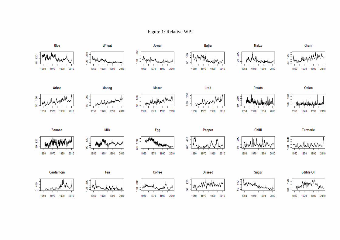
Figure 1: Relative WPI

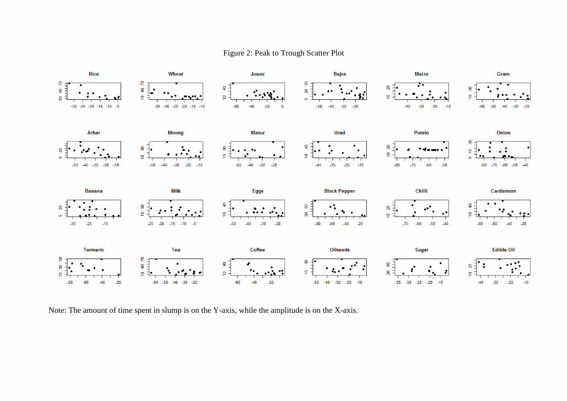
Figure 2: Peak to Trough Scatter Plot

Note: The amount of time spent in slump is on the Y-axis, while the amplitude is on the X-axis.

Figure 3: Trough to Peak Scatter Plot

Note: The amount of time spent in slump is on the Y-axis, while the amplitude is on the X-axis.

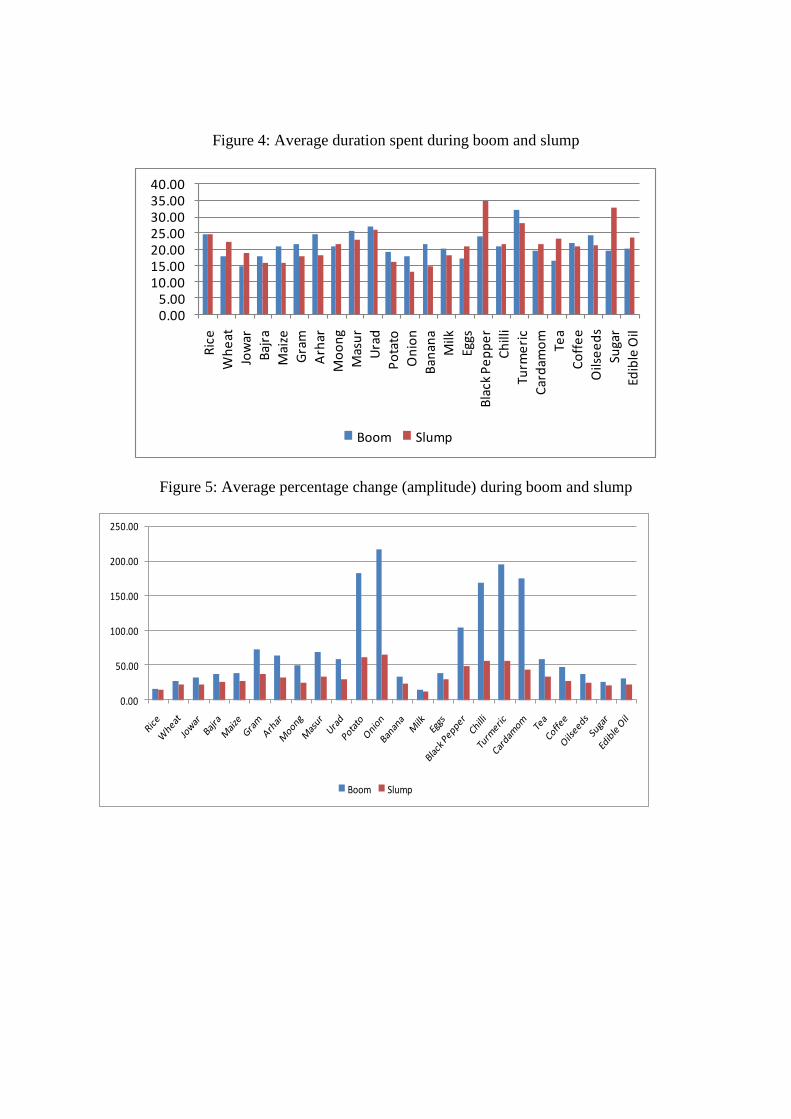
Figure 4: Average duration spent during boom and slump

0.005.00

10.0015.0020.0025.0030.0035.0040.00

Ric

e

Wh

eat

Jow

ar

Baj

ra

Mai

ze

Gra

m

Arh

ar

Mo

on

g

Mas

ur

Ura

d

Po

tato

On

ion

Ban

ana

Milk

Eggs

Bla

ck P

ep

pe

r

Ch

illi

Turm

eri

c

Car

dam

om

Tea

Co

ffe

e

Oils

ee

ds

Suga

r

Edib

le O

il

Boom Slump

Figure 5: Average percentage change (amplitude) during boom and slump

0.00

50.00

100.00

150.00

200.00

250.00

Boom Slump

Table 1: Commodity Classifications

Effective MSP Rice, Wheat

MSP exists

Jowar, Bajra, Maize, Gram, Arhar, Moong, Masur, Urad, Sugar, Oilseeds,

Edible Oil

Internationally

Traded

Black Pepper, Chillies, Turmeric, Cardamom, Tea, Coffee

Fruits and Vegetables Potato, Onion, Banana

Others Milk, Eggs

Table 2: Summary Statistics of the relative WPI series

N Mean Std. Dev. Skewness Kurtosis

Rice 773 110.48 11.43 0.34 2.47

Wheat 773 116.18 22.13 0.71 2.49

Jowar 773 101.85 18.52 0.37 2.50

Bajra 773 109.03 27.78 0.74 2.68

Maize 701 107.76 23.63 1.24 5.03

Gram 773 91.25 25.56 0.08 2.38

Arhar 769 109.29 30.01 0.39 2.95

Moong 701 108.75 32.80 0.80 4.32

Masur 701 101.80 26.96 0.55 3.11

Urad 701 135.68 39.02 0.78 3.23

Potato 701 144.72 51.06 0.79 3.67

Onion 701 107.15 46.77 2.78 16.94

Banana 701 104.89 13.94 0.14 2.42

Milk 701 110.79 8.65 0.38 3.74

Black Pepper 773 154.96 75.95 1.53 4.94

Chillies 773 102.45 31.12 1.24 5.21

Turmeric 773 230.91 108.32 1.77 7.83

Cardamom 701 212.35 153.50 1.26 4.12

Tea 773 133.40 39.16 1.79 8.79

Coffee 773 155.66 44.27 1.15 6.28

Oilseeds 773 96.11 13.25 0.04 3.36

Sugar 773 96.25 24.24 0.20 1.91

Edible Oil 701 92.29 15.94 0.20 2.36

Note: N is for the no. of observation or months. Std. Dev. Refers to the standard

Deviation.

Table 3: Unit Root Tests Statistics

Without Trend With Trend

ADF PP ADF PP

Rice -2.005 -2.459

-3.321* -3.883**

Wheat -2.039 -2.397

-3.344* -4.033***

Jowar -2.947** -3.559***

-3.035 -3.919**

Bajra -2.556 -3.136**

-3.279* -4.257***

Maize -2.797* -3.425**

-3.543** -4.455***

Gram -2.135 -3.134**

-3.394* -4.695***

Arhar -2.152 -2.848*

-3.703** -4.681***

Moong -1.463 -2.092

-3.601** -4.677***

Masur -2.343 -2.830*

-3.617** -4.477***

Urad -1.414 -2.129

-2.754 -3.846**

Potato -4.235*** -5.147***

-4.834*** -5.873***

Onion -6.362*** -6.860***

-6.688*** -7.202***

Banana -6.133*** -5.717***

-7.167*** -6.906***

Milk -4.811*** -4.059***

-4.812*** -4.060***

Eggs -1.655 -1.126

-4.773*** -3.868**

Black Pepper -1.662 -2.270

-1.683 -2.288

Chillies -3.328** -5.076

-3.342* -5.098***

Turmeric -2.02 -3.179**

-2.315 -3.425**

Cardamom -2.155 -2.364

-3.046 -3.402*

Tea -3.503*** -3.500***

-4.190*** -4.266***

Coffee -2.168 -2.649*

-2.180 -2.656

Oilseeds -3.595*** -4.794

-3.603** -4.807***

Sugar -2.356 -2.285

-3.319* -3.261*

Edible Oil -2.011 -2.883** -2.978 -3.877**

Note: ***, ** and * represent significance at1, 5 and 10 percent respectively.

Table 4: Zivot-Andrews unit root test results

Both trend and

Intercept Trend

Intercept

BP t-statistic

BP t-statistic

BP t-statistic Lags

Rice 07:1975 -4.903

12:1998 -4.085

07:1975 -4.891** 4

Wheat 03:1979 -5.884***

02:1987 -5.419***

03:1996 -5.623*** 5

Jowar 08:1976 -5.928***

11:1987 -5.499***

06:1975 -5.753*** 5

Bajra 05:1975 -7.564***

12:2001 -5.611***

05:1975 -7.468*** 5

Maize 02:1975 -6.442***

08:1965 -5.275***

09:1975 -5.952*** 5

Gram 11:1963 -6.656***

05:2001 -6.113***

11:1963 -6.394*** 4

Arhar 11:1999 -5.915***

06:1995 -5.469***

11:1999 -5.879*** 5

Moong 07:1973 -6.055***

01:1965 -5.69***

09:1963 -5.758*** 4

Masur 03:1968 -5.943***

11:1964 -4.879**

05:1962 -4.966** 3

Urad 12:1972 -5.504**

12:1965 -4.813**

10:1956 -5.037** 5

Potato 04:1974 -7.22***

06:1984 -

6.924*** 12:1970 -7.201*** 4

Onion 02:1980 -10.046***

11:2002 -9.881***

02:1980 -9.948*** 1

Banana 07:1974 -6.125***

08:1967 -5.379***

05:1977 -5.921*** 5

Milk 03:1976 -3.869

11:1967 -3.065

03:1976 -3.616 3

Eggs 11:1973 -4.099

11:2002 -3.118

11:1973 -4.038 4

Black Pepper 08:1959 -4.283

05:1957 -4.436**

11:1983 -3.458 5

Chillies 12:1978 -7.4***

07:1969 -

7.231*** 12:1978 -7.409*** 5

Turmeric 02:1959 -5.139**

02:1957 -

5.057*** 06:1982 -5.058** 5

Cardamom 06:1983 -5.263**

06:1990 -3.435

05:1983 -5.054** 5

Tea 01:1983 -5.04

01:1969 -4.483**

01:1983 -5.061** 4

Coffee 01:2000 -3.293

01:1957 -2.688

11:1998 -2.876 1

Oilseeds 12:1995 -6.037***

12:2001 -

5.937*** 09:1975 -5.929*** 5

Sugar 12:1991 -5.223**

09:1985 -4.419

12:1991 -5.222 4

Edible Oil 01:1982 -5.731***

03:1970 -

5.071*** 11:1981 -5.684*** 5

Note: The critical values are -5.57 and -5.08 at 1 and 5 percent respectively. * and **

represent significance at 5 and 1 percent respectively. BP implies the break point dates.

Table 5: Regression Results

Constant Trend Level dummy Slope dummy R2

Rice 2.08999*** -0.00004*** -0.05132***

0.57

(927.7) (-4.34) (-12.27)

Wheat 2.23463*** -0.00046*** 0.09182*** -0.00206 0.73

(513.9) (-30.06) (14.55) (-0.3)

Jowar 2.08962*** -0.00003 -0.12500*** 0.02532*** 0.47

(353.45) (-1.31) (-13.39) (2.83)

Bajra 2.13127*** 0.00001 -0.17497*** -0.02418*** 0.68

(402.42) (0.5) (-18.75) (-2.87)

Maize 2.09616*** -0.00014*** -0.12531*** 0.08196*** 0.61

(392.74) (-7.06) (-15.88) (11.45)

Gram 1.77042*** 0.00025*** 0.08646*** 0.01375 0.53

(259.89) (8.61) (7.11) (1.12)

Arhar 1.83114*** 0.00049*** -0.15286*** 0.06440*** 0.65

(300.77) (27.43) (-12.93) (5.43)

Moong 1.76987*** 0.00049*** 0.06051*** -0.01337 0.75

(282.88) (28.93) (3.48) (-0.77)

Masur 1.78892*** 0.00037*** 0.04775*** 0.00829 0.62

(252.52) (20.34) (3.29) (0.58)

Urad 1.88990*** 0.00041*** 0.02325* 0.03764*** 0.65

(171.26) (21.46) (1.8) (3.85)

Potato 2.22530*** 0.00010** -0.16870*** -0.04285*** 0.33

(187.22) (2.08) (-11.4) (-2.61)

Onion 1.89802*** 0.00036*** -0.10636*** 0.03049* 0.12

(124.31) (6.29) (-5.28) (1.69)

Banana 1.93952*** 0.00021*** -0.07110*** 0.03763*** 0.38

(468.59) (12.89) (-11.45) (6.76)

Milk 2.04188*** 0.00000

0.00

(727.48) (-0.48)

Eggs 2.34660*** -0.00066***

0.87

(517.58) (-69.26)

Black Pepper 2.31621*** 0.00045***

-0.37677*** 0.05

(141.89) (-12.32)

(-16.59)

Chillies 1.94333*** 0.00014*** -0.09749*** 0.05482*** 0.06

(196.31) (3.08) (-5.46) (3.31)

Turmeric 2.33471*** 0.00026*** 0.054407** -0.16013*** 0.15

(148.69) (3.86) (2.11) (-6.96)

Cardamom 1.94464*** 0.00013** 0.45480***

0.66

(100.57) (1.96) (16.85)

Tea 2.28666*** -0.00053*** 0.16666*** -0.05061*** 0.52

(337.77) (-15.32) (14.22) (-4.63)

Coffee

Oilseeds 1.99847*** 0.00003** -0.03543*** 0.01727*** 0.07

(521.16) (1.98) (-5.27) (2.85)

Sugar 2.09907 -0.00058*** 0.12888***

0.80

(560.44) (-48.83) (-22.28)

Edible Oil 1.99920*** -0.00003* -0.11746*** 0.04610*** 0.52

(472.53) (-1.79) (-16.11) (6.72)

Note: ***, ** and * represent the significance at 5, 10 and 1 percent respectively. Figures in

the parentheses are the respective t-value of the coefficients.

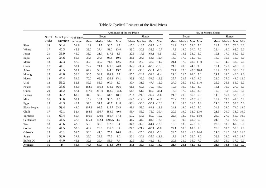
Table 6: Cyclical Features of the Real Prices

Mean Median Max Min Mean Median Max Min Mean Median Max Min Mean Median Max Min Rice 14 50.4 51.9 16.9 17.7 33.5 1.7 -15.3 -13.7 -32.7 -4.2 24.9 22.0 53.0 7.0 24.7 17.0 70.0 8.0 Wheat 17 40.3 45.8 28.0 27.4 51.2 13.0 -23.2 -20.8 -38.5 -10.7 17.9 18.0 30.0 7.0 22.4 16.0 68.0 6.0 Jowar 21 33.9 45.0 33.0 21.7 117.2 3.6 -22.5 -17.5 -64.1 0.2 15.0 14.5 33.0 5.0 19.1 17.0 54.0 6.0 Bajra 21 34.6 50.5 37.8 27.8 93.8 10.6 -26.6 -24.3 -53.6 -12.4 18.0 17.0 32.0 6.0 16.9 15.5 35.0 6.0 Maize 18 37.3 57.0 39.5 38.7 71.8 12.5 -28.0 -28.9 -47.9 -11.2 21.1 17.0 40.0 11.0 15.9 14.5 32.0 7.0 Gram 17 41.1 53.1 72.2 74.1 121.8 24.8 -37.7 -38.4 -63.0 -18.3 21.6 20.0 44.0 9.0 19.1 15.0 43.0 5.0 Arhar 17 43.5 57.4 64.4 56.3 144.6 13.7 -33.3 -36.8 -56.1 -7.3 24.7 27.0 42.0 10.0 18.4 19.0 38.0 5.0 Moong 15 43.0 50.8 50.5 54.1 109.2 5.7 -25.5 -24.1 -51.3 -9.4 21.0 21.5 68.0 7.0 21.7 18.0 46.0 9.0 Masur 13 47.4 54.6 70.0 68.5 136.3 13.1 -33.9 -36.2 -54.6 -12.8 25.7 21.5 48.0 9.0 23.0 25.0 43.0 12.0 Urad 12 53.2 52.8 59.9 58.9 97.0 8.0 -30.4 -31.9 -47.7 -12.2 27.0 26.0 54.0 11.0 26.2 26.5 55.0 6.0 Potato 19 35.6 54.5 182.5 156.8 478.2 86.6 -61.6 -60.5 -79.9 -48.9 19.3 19.0 42.0 8.0 16.1 16.0 27.0 6.0 Onion 20 31.2 57.1 217.0 211.0 482.0 104.6 -64.9 -61.6 -85.0 -37.1 18.0 17.0 43.0 8.0 12.9 8.0 30.0 5.0 Banana 18 37.2 60.9 34.0 38.5 61.9 10.1 -23.8 -24.8 -37.2 -6.6 21.8 21.0 56.0 6.0 14.8 16.0 32.0 5.0 Milk 16 38.6 52.4 15.2 13.1 30.5 1.5 -12.5 -12.8 -24.6 -2.2 20.2 17.0 42.0 6.0 18.4 19.0 47.0 5.0 Eggs 15 48.3 46.7 39.0 37.7 63.7 11.8 -30.4 -30.8 -50.1 -16.8 17.4 18.0 31.0 7.0 21.0 17.0 53.0 5.0 Black Pepper 11 59.4 43.0 105.2 99.5 315.7 23.3 -48.6 -53.0 -84.1 -13.9 24.1 19.0 66.0 5.0 34.8 28.0 74.0 13.0 Chilli 17 42.1 51.4 168.6 136.7 384.9 49.0 -56.4 -55.2 -76.0 -39.4 20.9 19.0 32.0 13.0 21.5 20.0 38.0 10.0 Turmeric 11 60.4 55.7 196.0 170.9 380.7 37.3 -57.2 -57.6 -80.9 -19.2 32.3 33.0 50.0 14.0 28.0 27.0 50.0 10.0 Cardamom 16 41.5 47.3 175.1 102.4 1215.5 4.7 -44.2 -44.0 -81.3 -13.6 19.5 19.5 40.0 6.0 21.8 17.0 57.0 5.0 Tea 18 40.6 42.5 59.3 38.3 272.0 6.4 -34.1 -32.0 -64.4 -13.6 16.5 13.0 45.0 7.0 23.6 18.5 69.0 9.0 Coffee 16 41.5 52.9 48.4 28.6 235.5 6.4 -27.5 -21.4 -65.1 -6.0 22.1 18.0 63.0 5.0 20.9 18.0 55.0 7.0 Oilseeds 15 46.1 51.5 38.3 41.0 75.1 16.0 -24.4 -25.0 -51.2 -5.1 24.5 26.0 41.0 14.0 21.6 21.0 34.0 11.0 Sugar 13 53.0 39.3 26.0 23.3 77.3 8.0 -22.1 -20.1 -35.6 -11.9 19.8 18.0 36.0 8.0 32.8 28.0 69.0 14.0 Edible Oil 14 44.0 46.1 32.1 29.4 58.9 7.4 -22.3 -18.9 -41.2 -8.1 20.3 21.0 36.0 7.0 23.7 25.0 37.0 9.0 Average 16 44 50.8 75.4 65.5 212.8 20.0 -33.6 -32.9 -56.9 -14.2 21.4 20.1 44.5 8.2 21.6 19.3 48.2 7.7

Amplitude of the the Phase Slump % of Time

in Boom

Boom No. of Cycles

Slump Boom Mean Cycle Duration

No. of Months Spent

Appendix I

The Bry-Boschan procedure used here is the one used by Martin Everts in his paper

“Duration of Business Cycles”. We are grateful to Martin Everts for sharing with us the

MATLAB codes for this procedure. Description of the codes is as follows (as presented in

Everts (2006)):

1. Identifying and replacing extreme values using the Spencer Curve

2. Determination of cycles in a 12 months moving average

a. Find points higher or lower 5 months on each side

b. Enforce the conditions that peaks and troughs alternate

3. Identifying the corresponding turning points using the spencer curve after the extreme

values are replaced

a. Identifying the turning points as in step 2 within the new series over 5 months on

either side

b. Enforce the conditions that minimum cycle duration is 5 months by eliminating

shorter cycles

4. Determination of the corresponding turns in short-term moving average of 3 to 6

months depending upon the periods of cyclical dominance (PCD)

a. Identifying the turning points as in step 2 within the new series over 5 months on

either side in the spencer curve

5. Indentifying the turning points in the original data series

a. Identification of the highest (or lowest) value within the PCD term of the selected

turning points over 5 months on either side in the original data series

b. Enforce the conditions that peaks and troughs alternate

c. Ensure that troughs are less than the peaks

d. Eliminating cycles with phases less than 5 months

e. Eliminating cycles with duration less than 15 months

6. Statement of the final turning points