characterizing ambiguity attitudes using model uncertainty
TRANSCRIPT

HAL Id: hal-03031502https://hal.archives-ouvertes.fr/hal-03031502
Submitted on 26 Mar 2021
HAL is a multi-disciplinary open accessarchive for the deposit and dissemination of sci-entific research documents, whether they are pub-lished or not. The documents may come fromteaching and research institutions in France orabroad, or from public or private research centers.
L’archive ouverte pluridisciplinaire HAL, estdestinée au dépôt et à la diffusion de documentsscientifiques de niveau recherche, publiés ou non,émanant des établissements d’enseignement et derecherche français ou étrangers, des laboratoirespublics ou privés.
Characterizing ambiguity attitudes using modeluncertainty
Loïc Berger, Valentina Bosetti
To cite this version:Loïc Berger, Valentina Bosetti. Characterizing ambiguity attitudes using model uncertainty. Journalof Economic Behavior and Organization, Elsevier, 2020, 180, pp.621-637. �10.1016/j.jebo.2020.02.014�.�hal-03031502�

CHARACTERIZING AMBIGUITY ATTITUDES
USING MODEL UNCERTAINTY∗
Loıc Berger† Valentina Bosetti‡
Abstract
We report the results of an experiment eliciting individuals’ attitudes toward
risk and model uncertainty. Using a joint elicitation procedure, we then precisely
quantify the strength of individuals’ attitude toward ambiguity in the context of the
smooth model and characterize its main properties. Our results provide empirical
evidence of decreasing absolute ambiguity aversion (DAAA) and constant relative
ambiguity aversion (CRAA). These results shed new light on the way ambiguity
attitudes may affect important decisions, such as the choice of health insurance
policies or the optimal investment strategy in the face of climate change.
Keywords: Ambiguity aversion, Laboratory experiment, Non-expected utility, Sub-
jective probabilities, Decreasing absolute ambiguity aversion
JEL Classification: D81
∗We thank Mohammed Abdellaoui, Aurelien Baillon, Han Bleichrodt, Itzhak Gilboa, Glenn Harrison,Francois Pannequin, Massimo Tavoni, Peter Wakker and especially Massimo Marinacci for helpful com-ments and discussions. We acknowledge audiences at CEAR/MRIC Behavioral Insurance Workshop, theannual seminar of the European Group of Risk & Insurance Economists (EGRIE), the workshops “Un-certainty and public decision” (EconomiX) and seminar participants at Bocconi University, RotterdamUniversity, HEC Paris, Fondazione Eni Enrico Mattei, IESEG and EM-Lyon for their helpful comments.We thank Jacopo Crimi, Johannes Emmerling, Michele Peruzzi, Caterina Verrone and Stefano Zenobifor their help with the experiment. This work was supported by the European Union Seventh FrameworkProgramme FP7 [grant agreement no 308329 ADVANCE, ERC-2013-StG 336703-RISICO]; the AgenceNationale de la Recherche [grant ANR-17-CE03-0008-01 INDUCED]; the CASBS. Logistic support fromthe Bocconi Experimental Laboratory in the Social Sciences (BELSS) for hosting our experimental ses-sions is appreciated. Some results of this research have previously circulated in a working paper titled“Ellsberg Re-revisited: An Experiment Disentangling Model Uncertainty and Risk Aversion.”†CNRS, IESEG School of Management, Univ. Lille, UMR 9221 - LEM, F-59000 Lille, France; and
RFF-CMCC European Institute on Economics and the Environment (EIEE), Centro Euro-Mediterraneosui Cambiamenti Climatici, Italy. E-mail address: [email protected].‡Department of Economics and IGIER, Bocconi University; and and RFF-CMCC European Institute
on Economics and the Environment (EIEE), Centro Euro-Mediterraneo sui Cambiamenti Climatici, Italy.
1
Ambiguity may be high [...] when there are questions of reliability and
relevance of information, and particularly where there is conflicting
opinion and evidence. (Ellsberg, 1961, p. 659)
1 Introduction
Almost sixty years ago, Ellsberg (1961) proposed a series of experiments whose
results suggest that people generally prefer situations in which they know the prob-
ability of an event occurrence to situations in which this probability is unknown.
This behavior, which violates a key axiom of the classic model of choice under
uncertainty, is known as ambiguity aversion. It has been the focus of a large body
of research that has explored both the theoretical and experimental sides of the
topic. According to Ellsberg, this preference is due not to the relative desirabil-
ity of the possible payoffs, or the relative likelihood of the events affecting them,
but to the nature of the information about the relative likelihood of events. In
particular, Ellsberg (1961, p. 657) wrote:
What is at issue might be called the ambiguity of this information, a
quality depending on the amount, type, reliability and “unanimity”
of information, and giving rise to one’s degree of “confidence” in an
estimation of relative likelihoods.
Ambiguity aversion thus results from a preference for situations in which all events
relevant to decision-making are associated with obvious probability assignments,
in which everyone agrees (i.e. what is generally called “risk” in economics) to
situations in which some events do not have an obvious, unanimously agreeable
probability assignment (Ghirardato, 2004).
Ambiguity occurs in virtually all real-life situations. It plays a major role in
many problems policymakers and public authorities may face and thus directly
affects their decision-making processes. Ambiguity may, for example, result from
different opinions of experts about the probability of a particular event (Caban-
tous, 2007; Cabantous et al., 2011). It may also arise from multiple plausible
models predicting the probabilistic effects of alternative policies.
One area in which ambiguity frequently occurs is in health insurance (Gilboa
and Marinacci, 2013; Marinacci, 2015). Consider, for example, the problem of
a decision maker (DM) who must choose whether to buy insurance against the
risk of a heart disease. By browsing the Internet and providing some personal
information (e.g., age, cholesterol level, blood pressure, smoking habits), the DM
is confronted with different probability assessments of heart disease provided by
2

the risk calculators of different hospitals. Thus, different “experts”1 provide dif-
ferent probability models for the same event (i.e. suffering a heart attack in the
next years). As Gilboa and Marinacci (2013) illustrate, the estimates may vary
substantially from one expert to the other. The reason is that simple relative fre-
quencies cannot be used as a definition of the probability of a heart disease because
no two human bodies are perfectly identical. Instead, the calculators assess the
probabilities for different individuals depending on their characteristics using more
complex methods. As a consequence, the assessed probabilities are not perfectly
objective: the team in charge of the calculator in each hospital must choose the
individual characteristics to be used, the database, and the estimation technique.
Together, this results in a set of possible probability models rather than a unique
probability distribution.
Another example of ambiguity is environmental disasters for which policy-
makers may need to design an investment strategy, entailing both mitigation and
adaptation efforts in response to climate change.2 In this context, different proba-
bility distributions may exist to characterize the same event, such as temperature
response to cumulated emissions (Heal and Millner, 2014). This happens because
there is not enough information available; because different climate predictions
exist based on different data sets, different estimation techniques, or numerical
models exist; or because different experts provide different probabilities assess-
ments for the same occurrence. As a consequence, little is known about how,
for example, global warming will affect the probability of a climate catastrophe
(Lenton et al., 2008). As these events have not been encountered by humankind
before, their likelihood of occurrence is extremely difficult to quantify precisely.
Decisions are therefore generally made based on the advice of scientific experts
(e.g., Intergovernmental Panel on Climate Change) whose probability assessments
may vary significantly (Kriegler et al., 2009; Berger et al., 2017). In this case as
well, different probability models characterizing the same event exist.
Whether regarding health-related issues or environmental questions, what is
common to these examples is the idea that ambiguity and elements of insurance of
different types are tightly intertwined. Specifically, while the first example entails
the provision of market insurance in the presence of ambiguity, the second example
1Throughout the paper, we refer to experts as individuals or entities who presumably havemore information and/or expertise than the DM and who are acting as advisers by providinginformation (Budescu et al., 2003).
2Adaptation is the process of “adjustment to actual or expected climate and its effects. Inhuman systems, adaptation seeks to moderate harm or exploit beneficial opportunities” (IPCC,2014a), while mitigation is “a human intervention to reduce the sources or enhance the sinks ofgreenhouse gases” (IPCC, 2014b).
3

deals with ambiguity and self-insurance (SI)/self-protection (SP) in the sense of
Ehrlich and Becker (1972). These risk management tools are generally used to
deal with the risk of a monetary loss when market insurance is not available. In
both situations, the DM has the opportunity to undertake an effort to modify the
distribution of a potential negative outcome (loss). In the case of SI, the effort
is intended to reduce the size of the loss, while in the case of SP, the effort aims
to reduce the probability of suffering from the loss. In this sense, investments in
adaptation efforts in the face of climate change represent an example of SI, while
mitigation efforts correspond to SP (Berger, 2016).
To what extent do ambiguity preferences affect the decisions to purchase health
insurance policies or to undertake SI/SP efforts in the presence of climate change?
The answer to this question fundamentally depends on the strength of ambiguity
aversion, as well as on some behavioral properties of the function characterizing
ambiguity preferences. In theoretical works, using single-period models, Snow
(2011) and Alary et al. (2013) show that ambiguity aversion increases the insur-
ance coverage rate and the optimal level of SI, while it may increase or decrease
the optimal level of SP. In a two-period setting, Berger (2016) and Berger et al.
(2017) demonstrate that ambiguity aversion alone is not sufficient to sign the ef-
fect ambiguity has on the decision to (self-)insure or self-protect. An additional
condition of non-increasing absolute ambiguity aversion is also required in most
situations in which the degree of model disagreement among experts decreases
with the effort. Yet, at an empirical level, the question has not been tackled in
much detail.
The aim of this paper is to provide a methodological contribution to this lit-
erature. Specifically, what we propose herein is an experimental method capable
of quantifying more precisely the extent to which ambiguity aversion exists and
characterizing its main properties.3 To do so, we decompose ambiguity into two
distinct layers of analysis, following the approach of Hansen (2014), Marinacci
(2015) and Hansen and Marinacci (2016). The first layer, commonly referred to
as risk (or aleatory uncertainty), features the probability measure associated with
the randomness of an event. It refers to the physical quantification of uncertainty
by means of a probability model that fully specifies the outcome probabilities.
This layer of risk within a model is the one typically studied by economists in
problems involving decision-making under uncertainty (in the context of SI-SP,
see for example Dionne and Eeckhoudt, 1985; Jullien et al., 1999; Eeckhoudt and
3Few studies have actually attempted to quantify the strength of the ambiguity aversioneffect. Notable exceptions, using various models, are those of Abdellaoui et al. (2011); Ahn et al.(2014); Dimmock et al. (2016).
4

Gollier, 2005). The second layer, referred to as model uncertainty (or epistemic
uncertainty), represents uncertainty about which alternative probability model
should be used to assign probabilities.4 This layer of analysis occurs when the
correct risk is itself unknown. This is the case, for example, when multiple expert
assessments seem plausible in describing the randomness of a phenomenon.
In a controlled experimental environment that extends Holt and Laury’s (2002)
and Andersen et al.’s (2008) setups, we expose our subjects to various types of risk
and model uncertainty. Using the distinction between the two, our design enables
us to quantify precisely the degree of ambiguity aversion and to assess its main
properties by means of both non-parametric statistics and structural econometric
analyses of choice patterns.
Two main findings emerge from our analysis. First, subjects tend to be both
risk and model uncertainty averse but exhibit stronger aversion to model un-
certainty than to risk. This behavioral characteristic is evidence of ambiguity
aversion, which is then elicited through a joint estimation procedure. Second,
and analogously to what has been previously reported for risk aversion (Holt and
Laury, 2002, 2005), we find that model uncertainty aversion is decreasing when
considered in absolute terms and increasing when considered in relative terms. In
terms of ambiguity attitude, we find evidence of decreasing absolute ambiguity
aversion (DAAA) and constant relative ambiguity aversion (CRAA).
2 Experimental procedures
This section presents the procedures followed in the experiment. We analyze
two types of uncertain situations, represented by urns filled with balls that are ei-
ther red or black. The first situation is a simple risk situation in which the number
of red and black balls –and therefore the probability model– is objectively known.
The second situation is a model uncertainty situation in which ignorance is first
achieved by allowing both the number and the color of the balls in the urn to be
unknown before two experts provide their assessment –or probability models– of
the urn composition. In our experiment, the experts’ models always take the form
of precise probabilities that are distinct from each other.5 This situation presents
uncertainty in two layers: two possible models (the two experts’ assessments) rep-
4The term “ epistemic” derives from the Ancient Greek word ἐπισvτήμη, which means “knowl-edge”, while the term “aleatory”, which originates from the Latin alea, refers to any game ofchance involving dice.
5As Gajdos and Vergnaud (2013) note, it is not irrational to face two experts who providedistinct sets of predictions. In particular, this does not imply the presence of any asymmetry ofinformation.
5

resenting two distinct risks are provided to the subjects. The experiment consists
of a sequence of eight tasks. In each task, subjects are confronted with a series of
binary choices, presented in the form of ordered tables (see Holt and Laury, 2002).
2.1 The design
Each urn describes a particular type of uncertainty that we distinguish as
follows:
• Risk : the proportion of red and black balls in the urn is known;
• Model uncertainty : the proportion of red, black, and the total number of
balls in the urn are unknown. However, information is provided by two
“experts”, both giving their own assessment of the composition of the urn.
The probability of drawing a red (resp. black) ball P (r) (resp. P (b)) is thus
objectively known in the case of risk but not in the case of model uncertainty, in
which only information about the possible compositions of the urn is given.
CE tasks The first set of tasks takes the form of certainty equivalent (CE) tasks.
In these tasks, subjects make a series of choices between an uncertain prospect
and a sure amount of money. The uncertain prospect is represented by a risky
lottery in the first CE task and by a situation of model uncertainty in the second
CE task. Specifically, by letting X denote the set of monetary outcomes, and xpx
the binary lottery yielding x ≥ x ∈ X with probability p and x ∈ X otherwise,
subjects are tasked with making a series of 10 choices between xpx and different
values of x ∈ X ordered from x to x.6 In the case of model uncertainty, the lottery
xpx is replaced by the uncertain situation denoted xp1p2x, in which the subject
is only given the two experts’ assessed probabilities of winning p1 and p2. The
design of the CE tasks is standard and in accordance with the literature (see e.g.,
Abdellaoui et al., 2011). To our knowledge, these tasks have never been used in the
context of model uncertainty with experts. The CE tasks enable us to characterize
the payoff that would make the subject indifferent between the prospect and the
sure amount of money in both situations of risk and model uncertainty. These
CE tasks, which are extremely easy to understand from the subjects’ perspective,
help capture treatment effects and differences in individual preferences. They
provide a direct measure of the strength of model uncertainty aversion relative
to risk aversion without the need to rely on any specific model of choice. To
6We used the following values in our CE tasks: x = 25, x = 4, p = 0.5, and x ∈{25, 18, 15, 14, 13, 12, 10, 8, 6, 4}.
6

ease comparisons, we only consider the case of dogmatic experts in the CE tasks:
each expert’s assessment is degenerate in the sense that a probability of 100% is
associated with one of the two outcomes. This enables us to isolate the effect
of model uncertainty alone and to compare directly risk and model uncertainty
preferences.
Other PL tasks In the other tasks of the experiment, we use a double price list
(PL) procedure to jointly elicit risk and model uncertainty attitudes. We design
two risk tasks following Holt and Laury’s (2002) PL standard procedure,7 while in
the four remaining uncertain tasks, subjects make a series of choices between risk
situations xpx and situations of model uncertainty xp1p2x. Given the assumptions
of a particular model choice that we describe in Section 3, these tasks help us to
estimate, using econometric methods, the values of the curvature parameters of
two utility functions.
The randomness device As one of our main goals in the experiment is to
characterize the way individuals behave in the presence of model uncertainty,
we need to ensure that in the absence of experts’ information, subjects are in
a situation of ignorance. To mimic the situation of ignorance, we construct the
model uncertainty urn in such a way that the total number of balls in the urn
is itself unknown and number between 1 and 100. We call this modification of
Ellsberg’s (1961) canonical example, which reduces the information bias due to the
peculiarity of the urn representation, the randomness device. In such a situation,
the total number of potential objective models is 3045, which is the cardinality of
the Farey sequence of order 100 (see Berger, 2019).8
2.2 Discussion of the design
We aimed to develop a design that is simple but also emphasizes the difference
between risk and model uncertainty. The design presents a few caveats, which we
discuss here.
Elicitation procedure The PL procedure is one of the most commonly em-
ployed elicitation methods to represent choices between gambles (Andersen et al.,
7In each task, subjects are asked to make a series of 10 choices between two options (OptionA and Option B), each presenting a different lottery (for the full set of tasks, see the onlinesupplemental Appendix).
8A Farey sequence of order N , denoted FN , is the ascending series of irreducible fractionsbetween 0 and 1 whose denominators do not exceed N (Hardy et al., 1979).
7
2006). It is widely considered as an easy-to-explain and transparent procedure
that rarely confuses subjects about the incentives to respond truthfully (Harrison
and Rutstrom, 2008). However, it also has possible disadvantages. One of its
main drawbacks is that by being able to switch freely between the two options as
they progress down the decision tables, subjects may end up making inconsistent
choices either by switching more than once or by making reverse choices (Char-
ness et al., 2013). While we recognize that these inconsistent behaviors may be
problematic, given that they are difficult to rationalize under standard assump-
tions on preferences and the estimation technique and inference of risk and model
uncertainty attitudes require a unique switching point, we decided not to enforce
consistent choices in this experiment.9 Rather, we view the presence of such be-
havior as indicative of subjects failing to understand the instructions correctly or,
more generally, of confusion on their part. As a result, we discarded this incon-
sistent data from the analysis of our results. Another potential disadvantage is
that the PL procedure only elicits intervals from the subjects rather than point
estimates. In addition, it could induce subjects to pick a response in the middle of
the table, independent of their true values (framing effect), or it could be more ac-
curate in eliciting probability weighting than the curvature of the utility function
(for an in-depth discussion, see Andersen et al., 2006).
Model misspecification While two experts’ assessments were provided in the
model uncertainty tasks, these experts were not physically present in the lab during
the experiment. Although this situation is close to many real-life situations in
which experts’ opinions are presented without their physical presence, this feature
may have led subjects to downplay the experts’ opinions or to partially ignore
them. Given our design, we cannot guarantee that subjects were not considering
alternative models from the ones given by the experts when making their decisions
(i.e. misspecification issues). To minimize this potential bias, we proceeded in
two steps. First, we created an initial situation of ignorance using the randomness
device discussed in the previous section. This device ensures that the DM has a
priori no information whatsoever about the possible probability models. Second,
we added the desired structural information by means of expert probability models.
To induce the subject to use this information, we gave particular attention to the
way we presented the experts and their assessments.10 We are confident that
9Several techniques that enforce consistency in subjects’ choices are available in the literature(see e.g., Andersen et al., 2006), but with the major drawback that they may significantly biasthe results (Charness et al., 2013).
10For that purpose, we specifically mentioned the following in the instructions: “These expertsare the best we could find for this situation. They are both experienced and have excellent track
8
most of our subjects incorporated the information provided when making their
choices. We are indeed able to show that subjects’ choices monotonically follow the
stochastic dominance criteria induced by the changes in assessments provided by
the two experts (see Section 4.2.2). Relatedly, it could be argued that the absence
of physical experts in the room deceived our subjects, who were then tempted to
suspect or mistrust the whole experiment.11 Again, we are able to show that this
suspicion argument is inconsistent with the data we collected. However, to be on
the safe side, we explicitly indicated the following in the instructions read aloud
at the beginning of the experiment: “This experiment is about decision-making.
There will be no deception in the experiment.”
2.3 Recruitment and administration
The laboratory experiment took place at Bocconi University (Italy). We re-
cruited 189 subjects through an internal experimental economics recruitment sys-
tem. Each subject was authorized to participate only once and had to sign up
in advance for a particular time slot. The experiment was organized into 12 ses-
sions taking place over four days. Each session lasted approximately 75 minutes
and comprised between 13 and 19 subjects. Subjects were provided with paper,
pen, and a calculator. A session typically started with silent reading of general
instructions, which were printed and provided to each subject in the cubicle to
which he or she was assigned. The experimenter then read once more the in-
structions aloud and made sure everything was clear before the subjects began a
computerized training session that introduced them to the concepts of risk, model
uncertainty and decision tables. The experiment was then performed on comput-
ers, with the order of tasks randomized. Overall, the different tasks constituting
our experiment were associated with a random incentive system to determine the
records”.11While most experimental economists agree that deception should be avoided, nobody knows
exactly and with certainty what deception is and is not (Krawczyk et al., 2013). Yet a consen-sus has emerged across disciplines that deception involves intentional and explicit provision ofmisinformation (Hertwig and Ortmann, 2008). For example, Adair et al. (1985) define decep-tion as “the provision of information that actively misled subjects regarding some aspect of thestudy”, while Menges (1973) talks about instances in which “the subject is given misleading orerroneous information”. The main argument against the use of deception is that it jeopardizesfuture experiments if the subjects ever find out that they were deceived and report this informa-tion to their friends. Banning deception therefore ensures that negative reputational spillovereffects are avoided and maintains a “reputation among the student population for honesty inorder to ensure that subject actions are motivated by the induced monetary rewards rather thanby psychological reactions to suspected manipulation” (Davis and Holt, 1993). In this sense,our design was not subject to deception. In practice indeed, the way we constructed the modeluncertainty urn is by randomly selecting one of the two models introduced by the experts in thedesign, and implementing her assessment.
9

final payoff. After all subjects had answered all the questions, they filled out a
short socio-economic questionnaire before being told their payoffs (i.e. which of
their decisions had been randomly selected, what was the color of the ball drawn
from the urn they chose (if any), and what was the corresponding amount they
won). Subjects were then paid in cash a e5 participation fee and the additional
amount (up to e35) won depending on the choices they made. The average gain
was approximately e18.50 per subject. We conducted the lab experiment using
the experiment software z-Tree (Fischbacher, 2007). Details of the experimental
procedure and instructions are available in the online Supplemental Material.
3 Theoretical predictions
In this section, we present our theoretical predictions. We use a specific model
of choice proposed by Marinacci (2015) building on the work of Klibanoff et al.
(2005). This model, known as the smooth ambiguity model, is fairly general. It
enriches many of the recent theories of choice under uncertainty in cases in which
information is incorporated in the decision problem, while distinguishing between
the notions of aleatory and epistemic uncertainty.
3.1 The smooth ambiguity model
The DM evaluates acts f whose outcome depends on the realization of an
observable state. For each decision, the state may be associated with the color
c ∈ {r, b} of the ball (red r or black b) drawn from the urn under consideration.
In other words, each draw represents the realization of a random variable that
is characterized by an objective probability distribution, or model, corresponding
to a specific composition of the urn. For a given model, the uncertainty about
the outcome is of the aleatory type and is generally called risk in economics.12
Conditional on the model, the probability of drawing a red (black) ball is therefore
objective and refers to a physical concept (in this case, the composition of the urn).
As in many real-life decision problems, however, multiple possible compositions
of the urn may exist, and the DM is uncertain about which is the correct one. In
this case, the probability model generating the observations is itself uncertain.
Following the ex ante information, the DM is able to posit a set of potential
models describing the likelihoods of the different states. We assume that this set
M of possible compositions of the urn is consistent with the available information
12Other denominations such as physical, objective, inside, or measurable uncertainty are alsopresent in the literature. All refer to situations in which the probability distribution is known.
10

provided by the experts. In accordance with Wald (1950), we take this as a datum
of the decision problem.13 In other words, the DM behaves as if she knows that
states are generated by a probability model that belongs to the collection M . This
therefore means that a second layer of uncertainty may add to the first layer of
risk. This additional layer is however not of the aleatory type. Instead, it is of an
epistemic nature: the DM does not know which is the most accurate model, and
the probability that may be attached to each of them is therefore nothing but a
representation of the DM’s degrees of belief. Together, this makes the situation
uncertain (or ambiguous) rather than risky. We refer to this situation as model
uncertainty. The smooth representation of preferences under model uncertainty
assumes that epistemic uncertainty is quantified through a single prior probability
measure over the setM of models (Marinacci, 2015). The different possible models,
which can be fully characterized by their probability of drawing a red ball, are
indexed by a parameter θ and noted by Pθ(r). The DM attaches a probability
µ(θ) to each, reflecting the personal information she has on their likelihood.14
The DM then chooses the act that maximizes her utility given by the two-stage
criterion:
U(f) = Eθ(v ◦ u−1)
∑c∈{r,b}
Pθ(c)u (f(c))
. (1)
In this expression, Eθ is the expectation operator taken over the prior distribution
(i.e. EθXθ =´MX(θ)dµ(θ)), u is the von Neumann and Morgenstern (1944) util-
ity function capturing the DM’s risk attitude (i.e. toward aleatory uncertainty),
and v captures the attitude toward model uncertainty (i.e. toward epistemic un-
certainty). These functions are assumed to be strictly increasing, continuous, and
cardinally unique. Criterion (1) may be interpreted as follows: in the first stage,
the DM evaluates the expected payoff per each possible model Pθ(r) and expresses
it in monetary terms through a CE cθ ≡ u−1(∑
c∈{r,b} Pθ(c)u (f(c)))
. These CEs
cθ represent the amount of money that would make the DM indifferent between
receiving such amount for sure and facing the risk associated with the model. One
CE cθ may be computed for each model. It only depends on risk attitude through
the function u: the more risk averse the DM is, the lower is cθ. In the second
stage, the DM addresses model uncertainty and summarizes the utility of the act
by evaluating a global expected payoff Eθv (cθ) across the CEs in line with her
13This set of models is analogous to what Ellsberg (1961) calls “reasonable” distributions inhis subjective setting. In general, the set M is non-singleton, and the true model is assumed tobelong to M (no misspecification issues).
14In this sense, the prior probability measure µ taken over the set of possible models is subjec-tive: it reflects “personal information on models that the DM may have, in addition to objectiveinformation M” (Cerreia-Vioglio et al., 2013, p. 6754).
11

attitude toward model uncertainty v and prior belief µ. Note that in the case in
which both attitudes toward the different types of uncertainty are identical (i.e.
whenever v is equal –up to an affine transformation– to u), we recover the classical
subjective expected utility model of Cerreia-Vioglio et al. (2013), which encom-
passes Savage’s (1954) model. Representation (1) therefore encompasses both the
Savagean subjective expected utility and the classical von Neumann-Morgernstern
(when M is a singleton) representations. When attitudes toward risk and model
uncertainty are different, representation (1) consists of a version of smooth ambi-
guity aversion (Klibanoff et al., 2005) in which the ambiguity aversion function is
recovered by letting φ ≡ v ◦ u−1. In this sense, the DM is ambiguity averse if she
is more averse to model uncertainty than to risk (i.e. v more concave than u).
3.2 Predictions
We now present the theoretical predictions for individual choices under risk
and model uncertainty. We are particularly interested in characterizing the prop-
erties of the two functions u and v representing attitudes toward different types of
uncertainty and in relating the smooth ambiguity model uncertainty framework
to previous results obtained in the literature.
Hypothesis 1. We expect subjects to be both risk and model uncertainty
averse, in the sense that they will generally prefer the degenerate lottery, giving∑c∈{r,b} P (c) f(c) with certainty, to any uncertain situation in which an act f
yields f(c) with (expected) probability P (c) ∀c ∈ {r, b}. By letting CR and CMU
denote the CEs under risk and model uncertainty, respectively defined as
CR ≡ u−1
∑c∈{r,b}
P (c) f(c)
, and (2)
CMU ≡ v−1
Eθ(v ◦ u−1)
∑c∈{r,b}
Pθ(c)u (f(c))
, (3)
and by letting C be the sure amount corresponding to the expected gain of the
prospect, we expect to observe:
C ≥ CR (4)
C ≥ CMU . (5)
12

Expressed in terms of functional properties, these equations simply become u′′ ≤ 0
and v′′ ≤ 0. While Hypothesis 1 is trivial and has been extensively documented
in the literature (Holt and Laury, 2002, 2005; Andersen et al., 2008), it is useful
for our test of whether ambiguity aversion may result from a stronger aversion to
model uncertainty than to risk.
Hypothesis 2. Considering the decomposition of ambiguity into risk and
model uncertainty, we expect subjects to prefer risk to model uncertainty, in ac-
cordance with the results of Ellsberg (1961). Furthermore, we predict that the
degree of model uncertainty aversion (and of ambiguity aversion) will be finite. In
other words, subjects will not behave according to a maxmin decision criterion in
the sense of Wald (1950). In terms of CEs, we can write these predictions (under
the assumption of equal expected values) as:
CR ≥ CMU > C, (6)
where C refers to the CE obtained under the worst possible model. In terms of
functions u and v, the first part of (6) simply means that v is more concave than
u, in the sense of Arrow-Pratt (i.e. −v′′
v′≥ −u′′
u′), while the second part translates
to −v′′
v′<∞.15
Hypothesis 3. In line with what is widely accepted in the risk theory litera-
ture, and given the similarity of our procedure to that used in Holt and Laury
(2002, 2005), we expect to observe decreasing absolute risk aversion (DARA) and
increasing relative risk aversion (IRRA) for both functions u and v.16 Specifi-
cally, by changing the values of the gains proposed and the probabilities that are
associated with these gains, we expect to observe:
∂
∂w0
[−u
′′(w0)
u′(w0)
]≤ 0 and
∂
∂w0
[−u
′′(w0)
u′(w0)w0
]≥ 0, (7)
where w0 denotes the individual’s wealth level, which is composed of the indi-
vidual’s background wealth ω and the expected gain in each lottery xpx: w0 =
15Or, equivalently, v−1(
Eθ(v ◦ u−1)(∑
c∈{ri,bi} Pθ(c)u (fi(c))))
>
u−1(
minθ∑c∈{ri,bi} Pθ(c)u (fi(c))
).
16To be completely precise, we should discuss “decreasing absolute model uncertainty aversion”and “increasing relative model uncertainty aversion” in the case of function v, but for the sakeof simplicity we refer to the widely used acronyms DARA and IRRA for the v function as well.While the DARA property is well accepted in the literature, the IRRA property is subject todebate when investigated outside the lab environment (Harrison et al., 2007; Brunnermeier andNagel, 2008; Chiappori and Paiella, 2011).
13

ω + px + (1 − p)x. Similarly, we translate the DARA and IRRA properties of
function v to :
∂
∂w1
[−v′′(w1)
v′(w1)
]≤ 0 and
∂
∂w1
[−v′′(w1)
v′(w1)w1
]≥ 0, (8)
where the individual’s wealth level w1, in situations of model uncertainty, is an
average of CE wealth levels under the two experts’ models.17
Hypothesis 4. Because ambiguity aversion in this setup results from the com-
bination of attitudes toward risk and model uncertainty, we can indirectly charac-
terize the properties of the ambiguity function φ. In particular, we are interested
in knowing whether the absolute ambiguity aversion is constant or whether it is
increasing or decreasing, in the sense that agents are willing to pay more or less to
remove all source of uncertainty as their level of expected utility increases. Con-
stant absolute ambiguity aversion (CAAA), as argued by Grant and Polak (2013),
is an implicit characteristic of many of the ambiguity models proposed in the theo-
retical literature. It is for example implicitly assumed in the models of Gilboa and
Schmeidler (1989); Hansen and Sargent (2001) and Maccheroni et al. (2006). By
contrast, DAAA is a condition that plays an important role in the determination
of the precautionary saving motive under ambiguity (Gierlinger and Gollier, 2008;
Berger, 2014), in the chances of survival of ambiguity-averse investors (Guerd-
jikova and Sciubba, 2015) or in the choice of optimal abatement policies under
scientific uncertainty (Berger et al., 2017). We therefore expect to observe
∂
∂U
[−φ
′′(U)
φ′(U)
]≤ 0, (9)
where U is the individual’s expected utility level when the probabilities given by
experts are averaged.18 (Note that the ambiguity function φ ≡ v ◦ u−1 is defined
over expected utilities, while u and v are defined over monetary outcomes.)
17More precisely, in the uncertain situation characterized by xp1p2x, w1 is computed as w1 =µ(1)u−1 (p1u(ω + x) + (1− p1)u(ω + x)) + µ(2)u−1 (p2u(ω + x) + (1− p2)u(ω + x)). It is thenincreasing in the background wealth ω, in the payoff outcomes o and o, and in the expert’sprobabilities p1 and p2.
18Baillon and Placido (2019) also tested the CAAA and DAAA hypotheses using probabilityequivalent tasks (which consist of finding the objective probability at which, for a given prize,a subject is indifferent between betting on the ambiguous event and betting on the objectiveprobability; see Dimmock et al., 2016). At the aggregate level, they found evidence supportingour hypothesis: CAAA was systematically rejected in favor of DAAA.
14

4 Results
In this section, we report the results of our experiment. Section 4.1 uses the
results of the CE tasks to present a model-free evaluation of attitudes toward
model uncertainty in comparison with risk attitudes. Section 4.2 then proposes
a parametric estimation of the smooth ambiguity model by proceeding in two
steps. Attitudes toward risk and model uncertainty are first elicited using a joint
estimation procedure and then combined to obtain an evaluation of ambiguity
attitudes. To facilitate the derivation of our results, we use the following two
assumptions.
Assumption 1: No model misspecification. The DM only considers the
models given by the experts.
We assume that the exogenously given set of possible models M is well-defined and
is not misspecified. As such, and in accordance with Marinacci (2015), we take
it as a datum of the decision problem.19 As already discussed in the presentation
of our design (see Section 2.2), we imposed this assumption, even though nothing
theoretically prevents our subjects from considering alternative models distinct
from those given by the experts when making their decisions. (Yet, as argued
previously, we did our best to avoid such a situation.) While this assumption is not
strictly necessary when experts are dogmatic, as in the CE tasks (see subsequently
and also Berger and Bosetti, 2019), it is required when a specific model of choice
under uncertainty is considered. (For experimental evidence on the role of model
misspecification, see Aydogan et al., 2018.)
Assumption 2: Symmetry. The DM considers the two experts symmetri-
cally.
Assumption 2 is akin the one generally imposed in Ellsberg’s (1961) type of ex-
periments. In our case, it states that DM is indifferent between betting on red
and betting on black when confronted with a model uncertainty situation in which
the probabilities given by the experts are symmetric (i.e. P1(c) = 1−P2(c) for all
c ∈ {r, b}). The symmetry assumption has been widely used in the literature and
empirically validated by Abdellaoui et al. (2011), Chew et al. (2017) and Epstein
19Marinacci (2015, p. 1013), takes the physical information M as a primitive of the decision-making problem and notes that “the DM knows that the true model m generating the statesbelongs to the posited collection M .”
15

and Halevy (2018). The assumption relies on the symmetry of information argu-
ment. Given that the information over the two experts is perfectly symmetric (the
experts only differentiate themselves by their names of “Expert 1” and “Expert
2” and their assessments of the urn composition), there is no reason a priori to
attach more weight to one than the other. The prior distribution over the models
we use reflects this symmetry, such that we have µ (1) = µ (2) = 1/2.
4.1 General results
The results from the CE tasks are general in that they characterize attitudes
toward risk and model uncertainty directly from the choices made by the subjects
in a model-free way. These results therefore do not necessarily rely on the smooth
representation of preferences that we discussed previously. The CE tasks enable
us to obtain a direct measure of the strength of model uncertainty aversion rela-
tive to risk aversion. By considering dogmatic experts (i.e. experts who assess a
probability 100% or 0% of winning), we can isolate the effect of model uncertainty
alone from risk aversion and capture directly model uncertainty preferences.20
Moreover, as noted previously, our Assumption 1 is not strictly necessary with
dogmatic experts, as their presence ensures that the results we obtain for model
uncertainty aversion are, at worst, underestimated.21
Table 1 reports the descriptive statistics of the CEs associated with the risk
and model uncertainty prospects (i.e. 25 124 and 251 04, respectively). We use the
decision item at which the subject switches from the sure outcome to the uncertain
prospect to approximate her CEs. Formally, for a subject who switches from the
sure outcome after line i ∈ {0, 1, ..., 10} in the decision table, the CE, CJ , for
J ∈ {R,MU}, is given by
CJ =
x1 + 1
2(x1 − x2) if i = 0
12(xi+1 + xi) if i ∈ {1, ..., 9}x10 − 1
2(x9 − x10) if i = 10
(10)
where i = 0 means that the subject chooses the uncertain situation already in the
20In the case of model uncertainty with dogmatic experts, the CE collapses to
CMU = v−1(∑
c∈{r,b}12v(f(c)
)), while the CE of the 50-50 risk situation is CR =
u−1(∑
c∈{r,b}12u(f(c)
)).
21Indeed, if subjects were to consider any alternative model other than those belonging to theexogenously given set M = {0, 1}, the preferences associated with the observed choices wouldneed to reflect a higher aversion to model uncertainty than what we present in what follows (asany other symmetric distribution consistent with Assumption 2 in the space of expected utilitieswould consist of a mean-preserving contraction of the dogmatic experts’ distribution).
16

first choice option, and i = 10 means that she always chooses the sure outcome.
The reported CEs therefore correspond to the midpoint between the highest out-
come for which the uncertain prospect is preferred and the lowest outcome that is
preferred to the uncertain prospect. The consistent sub-sample contains 169 sub-
jects. As Table 1 shows, the results confirm our first two hypotheses: in general,
Table 1: Descriptive Statistics of the CEs
Mean Std. Error Median Min Max Obs.
CR 12.57 0.17 13.5 7 16.5 169
CMU 11.04 0.24 11 3 28.5 169
subjects are ready to pay a higher premium, measured as the difference between
the expected gain and the CE (C − CJ), to avoid a situation characterized by
epistemic uncertainty than to avoid a situation characterized by aleatory uncer-
tainty. In particular, for an expected outcome C = 14.5, the mean amount that
the subjects deem equivalent to the risk situation is CR = 12.6, while under model
uncertainty, it is CMU = 11. The difference between the CEs (CR − CMU) is sig-
nificantly positive (p-value=8.9e-11), and both are higher than the CE obtained
under the worst possible model C = 4.
The distribution of CR second order stochastically dominates that of CMU .
While CR does not first order stochastically dominate (FOSD) CMU , this is only
because one subject systematically preferred the model uncertainty situation to
the sure outcome (even when the choice was made between e25 for sure and a
situation in which one expert expressed a 100% probability that the gain is e25,
when the other expert expressed a 100% probability that the gain is e4). We
can only speculate what the preferences of this subject are. He or she could be
optimistic and always trust the expert predicting the highest outcome. In this
sense, the first choice would express indifference between two situations yielding
e25. After we remove this subject from the sample, we recover the result that
CR FOSD CMU . We illustrate this result in Figure 1 and Table 3, which display
the proportions of safe choices, expressed by preference for the sure amount, for
each of the 10 decisions in the risk and model uncertainty situations, respectively.
The dashed line represents the prediction under the assumption of neutrality (to
either risk or model uncertainty). In this case, the CEs of both situations are the
same, and the probability that the sure outcome is chosen is 1 for the first three
decisions and 0 for the remaining ones. The blue line presents the observed choice
frequency of the sure outcome option in the risk situation. As the figure shows, this
17

Figure 1: Proportion of safe choices in the CE tasks
1 2 3 4 5 6 7 8 9 100
10
20
30
40
50
60
70
80
90
100
Decision
Pro
port
ion o
f sa
fe c
ho
ices (
%)
risk
model uncertainty
prediction neutrality
outcome is at the right of the risk-neutral prediction, indicating a tendency for risk
aversion among subjects (CR ≤ C). The red line represents the observed frequency
in the case of model uncertainty and suggests that the subjects manifest a stronger
aversion to model uncertainty than to risk (CMU ≤ CR ≤ C). Finally, the subjects
did not express extreme model uncertainty aversion (which would have consisted
of a proportion safe choice of 100% for each decision). Only two subjects (i.e.
1.2% of the sample) expressed an extreme form of pessimism by systematically
selecting the certain outcome when confronted with model uncertainty.22 We
can therefore confidently reject the maxmin expected utility hypothesis in which
subjects only consider the worst possible model (Wald, 1950). A Wilcoxon signed-
rank test statistically confirms (p-value=3.2e-12) that the risk alternative is valued
differently than the corresponding model uncertainty prospect.23
At the individual level, we show, in Table 2, that 52% (resp. 37%, 11%) of the
sample expressed a stronger (resp. equal, weaker) aversion to model uncertainty
than to risk. These proportions’ difference is statistically significant. In line with
the theoretical model presented previously, these subjects are exhibiting ambiguity
aversion, neutrality, and loving, respectively.
22A looser definition of extreme pessimism, which treats subjects who expressed nine safechoices before switching to the model uncertainty situation as indifferent between the two options,leads to 5.3% of of individuals with extreme model uncertainty aversion.
23The significance of the one-sided test, in which the alternative hypothesis is that the medianof the switching point in the model uncertainty task is greater than in the risk aversion task, is4.2e-12.
18

Table 2: Comparison between attitudes toward risk and model uncertainty
CR < CMU CR = CMU CR > CMU Total
Count 19 62 88 169(Relative frequency) (11.2%) (36.7%) (52.1%) (100%)
Anticipating the parametric analysis developed in the next section, Table 3
provides the implied interval for the parameters of risk or model uncertainty aver-
sion in the context of the smooth model. For this exercise, we consider the special
case of power (CRRA)24 functions. Using an estimation procedure (described
Table 3: Classification of choices (CE tasks)
Numberof safechoices
Range of relative risk or modeluncertainty aversion:
u(x) or v(x) = x1−r/1− r
Proportion of choices
Risk ModelUncertainty
0-1 r < −1.04 0.00 % 0.59 %2 −1.04 < r < −0.12 0.56 % 0.59 %3 −0.12 < r < 0.12 34.91 % 17.75 %4 0.12 < r < 0.34 17.16 % 8.28 %5 0.34 < r < 0.55 18.34 % 15.38 %6 0.55 < r < 1 14.20 % 20.71 %7 1 < r < 1.55 10.06 % 21.89 %8 1.55 < r < 2.58 4.73 % 9.47 %
9-10 2.58 < r 0.00 % 5.33 %
next), we also find the best estimates for the coefficients of relative risk and model
uncertainty aversion when both u and v are of a CRRA type to be respectively
ru = 0.42 and rv = 0.83 in the CE tasks.
4.2 Characterizing smooth preferences
In this section, we use the choices made in the CE and PL tasks to further
characterize preferences under uncertainty in the context of the smooth ambiguity
model. In particular, we use the 80 binary choices each subject typically provided
to infer attitudes toward risk and model uncertainty, and then we use this infor-
mation to quantify the degree of ambiguity aversion. In total, 14% of the choices
made in the eight PL tasks were deemed inconsistent (reverse choices or multiple
24A utility function has the CRRA property if it takes the form u(x) = x1−r
1−r , where r is thecoefficient of relative risk aversion (when r = 1, this collapses to u(x) = lnx).
19

switching points) and were discarded from the analysis. This is in line with what
has previously been reported in other experiments (Holt and Laury, 2002).
4.2.1 Preliminary comment
As the smooth ambiguity model we test involves two distinct behavioral char-
acteristics (i.e. risk and model uncertainty attitudes), the experimental procedure
must be designed such that it generates data that are rich enough to disentangle
the different components and ultimately allow for estimating the subjects’ atti-
tude toward ambiguity. The double PL procedure, which presents choices in the
presence of both aleatory and epistemic uncertainty, is designed for this purpose.
It enables us to jointly elicit risk and model uncertainty attitudes. To under-
stand the importance of using a joint procedure, consider the identification of risk
and model uncertainty under the smooth model. Assuming that expression (1)
correctly describes preferences over uncertain alternatives, a subject is indifferent
between two options xpx and xp1p2x if and only if:
(v ◦ u−1)(pu(ω + x) + (1− p)u(ω + x)
)=
1
2
(v ◦ u−1
) (p1u(ω + x) + (1− p1)u(ω + x)
)+
1
2
(v ◦ u−1
) (p2u(ω + x) + (1− p2)u(ω + x)
),
(11)
where ω represents background wealth. When considered in terms of attitude
toward ambiguity, the identity φ ≡ v ◦ u−1 enables us to rewrite (11) as
φ(pu(ω + x) + (1− p)u(ω + x)
)=
1
2φ(p1u(ω + x) + (1− p1)u(ω + x)
)+
1
2φ(p2u(ω + x) + (1− p2)u(ω + x)
).
(12)
From (11) and (12), it is clear that estimating model uncertainty aversion (v)
or ambiguity aversion (φ) under the assumption of risk neutrality (u linear) will
yield the same result. Ambiguity aversion is therefore significantly overestimated
when risk neutrality is assumed.25 If we relax the assumption of risk neutrality
and let risk aversion −u′′/u′ be different than zero, it becomes clear from the
relationship −φ′′/φ′ = (−v′′/v′ + u′′/u′)/u′ that the implied degree of absolute
ambiguity aversion is lower. Therefore, we cannot capture the distinction between
model uncertainty and ambiguity aversion without estimating the level of risk
aversion, for which separated risk tasks also need to be performed.
25We discuss the estimation results of this particular case in the Appendix.
20
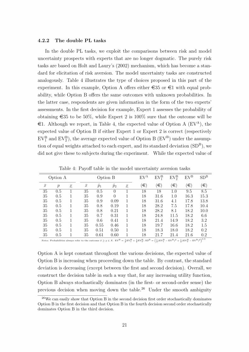
4.2.2 The double PL tasks
In the double PL tasks, we exploit the comparisons between risk and model
uncertainty prospects with experts that are no longer dogmatic. The purely risk
tasks are based on Holt and Laury’s (2002) mechanism, which has become a stan-
dard for elicitation of risk aversion. The model uncertainty tasks are constructed
analogously. Table 4 illustrates the type of choices proposed in this part of the
experiment. In this example, Option A offers either e35 or e1 with equal prob-
ability, while Option B offers the same outcomes with unknown probabilities. In
the latter case, respondents are given information in the form of the two experts’
assessments. In the first decision for example, Expert 1 assesses the probability of
obtaining e35 to be 50%, while Expert 2 is 100% sure that the outcome will be
e1. Although we report, in Table 4, the expected value of Option A (EVA), the
expected value of Option B if either Expert 1 or Expert 2 is correct (respectively
EVB1 and EVB
2 ), the average expected value of Option B (EVB) under the assump-
tion of equal weights attached to each expert, and its standard deviation (SDB), we
did not give these to subjects during the experiment. While the expected value of
Table 4: Payoff table in the model uncertainty aversion tasks
Option A Option B EVA EVB1 EVB
2 EVB SDB
x p x x p1 p2 x (e) (e) (e) (e) (e)
35 0.5 1 35 0.5 0 1 18 18 1.0 9.5 8.535 0.5 1 35 0.9 0 1 18 31.6 1.0 16.3 15.335 0.5 1 35 0.9 0.09 1 18 31.6 4.1 17.8 13.835 0.5 1 35 0.8 0.19 1 18 28.2 7.5 17.8 10.435 0.5 1 35 0.8 0.21 1 18 28.2 8.1 18.2 10.035 0.5 1 35 0.7 0.31 1 18 24.8 11.5 18.2 6.635 0.5 1 35 0.6 0.41 1 18 21.4 14.9 18.2 3.235 0.5 1 35 0.55 0.46 1 18 19.7 16.6 18.2 1.535 0.5 1 35 0.51 0.50 1 18 18.3 18.0 18.2 0.235 0.5 1 35 0.61 0.60 1 18 21.7 21.4 21.6 0.2
Notes: Probabilities always refer to the outcome x ≥ x ∈ X. EVB = 12
EVB1 + 1
2EVB
2 ; SDB =(
12
(EVB1 − EVB)2 + 1
2(EVB
2 − EVB)2)0.5
Option A is kept constant throughout the various decisions, the expected value of
Option B is increasing when proceeding down the table. By contrast, the standard
deviation is decreasing (except between the first and second decision). Overall, we
construct the decision table in such a way that, for any increasing utility function,
Option B always stochastically dominates (in the first- or second-order sense) the
previous decision when moving down the table.26 Under the smooth ambiguity
26We can easily show that Option B in the second decision first order stochastically dominatesOption B in the first decision and that Option B in the fourth decision second order stochasticallydominates Option B in the third decision.
21
model, this feature should induce subjects to switch only once, from Option A to
Option B, while progressing down the table. The subjects engaged in four tasks,
similar to that illustrated in Table 4, that varied in the proposed payoffs and prob-
abilities. For the set of payoffs and probabilities, the final payoffs span the range
of income over which we are estimating model uncertainty aversion, which is the
same as that over which risk aversion is estimated.27
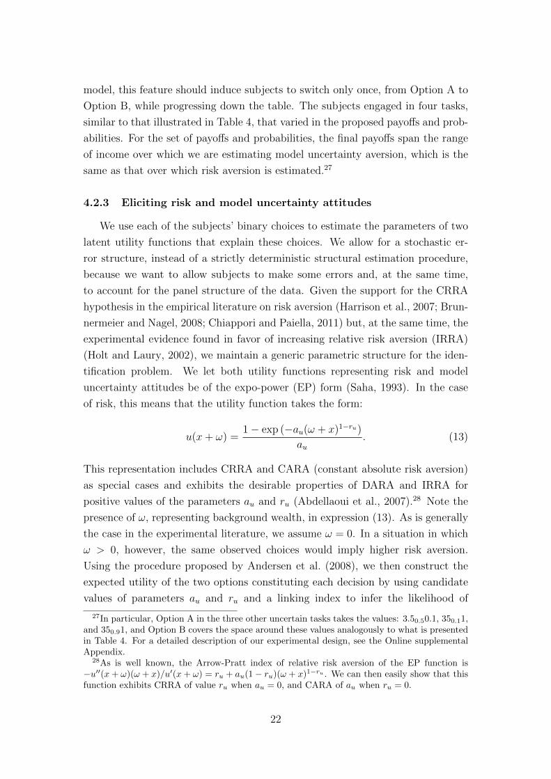
4.2.3 Eliciting risk and model uncertainty attitudes
We use each of the subjects’ binary choices to estimate the parameters of two
latent utility functions that explain these choices. We allow for a stochastic er-
ror structure, instead of a strictly deterministic structural estimation procedure,
because we want to allow subjects to make some errors and, at the same time,
to account for the panel structure of the data. Given the support for the CRRA
hypothesis in the empirical literature on risk aversion (Harrison et al., 2007; Brun-
nermeier and Nagel, 2008; Chiappori and Paiella, 2011) but, at the same time, the
experimental evidence found in favor of increasing relative risk aversion (IRRA)
(Holt and Laury, 2002), we maintain a generic parametric structure for the iden-
tification problem. We let both utility functions representing risk and model
uncertainty attitudes be of the expo-power (EP) form (Saha, 1993). In the case
of risk, this means that the utility function takes the form:
u(x+ ω) =1− exp (−au(ω + x)1−ru)
au. (13)
This representation includes CRRA and CARA (constant absolute risk aversion)
as special cases and exhibits the desirable properties of DARA and IRRA for
positive values of the parameters au and ru (Abdellaoui et al., 2007).28 Note the
presence of ω, representing background wealth, in expression (13). As is generally
the case in the experimental literature, we assume ω = 0. In a situation in which
ω > 0, however, the same observed choices would imply higher risk aversion.
Using the procedure proposed by Andersen et al. (2008), we then construct the
expected utility of the two options constituting each decision by using candidate
values of parameters au and ru and a linking index to infer the likelihood of
27In particular, Option A in the three other uncertain tasks takes the values: 3.50.50.1, 350.11,and 350.91, and Option B covers the space around these values analogously to what is presentedin Table 4. For a detailed description of our experimental design, see the Online supplementalAppendix.
28As is well known, the Arrow-Pratt index of relative risk aversion of the EP function is−u′′(x+ ω)(ω + x)/u′(x+ ω) = ru + au(1− ru)(ω + x)1−ru . We can then easily show that thisfunction exhibits CRRA of value ru when au = 0, and CARA of au when ru = 0.
22

the observed choice. The parameters of the latent utility function (13) are then
chosen to maximize the likelihood of obtaining the observed ranking of the different
options, taking into account a Luce (1959) error specification with a structural
noise parameter.29
The first part of Table 5 presents the estimates obtained from the risk tasks.
Given the prominent position CRRA has achieved in the theoretical and empirical
literature, we provide both the estimates for the cases in which u is of the CRRA
and EP type. The estimate of the CRRA parameter we obtain is 0.28, which is
Table 5: Estimates of risk, model uncertainty, and ambiguity preferences
u v φ
CRRA EP CRRA EP CRAA EP
a0.0294∗∗∗ 0.152∗∗∗ -1.802(0.00215) (0.0542) (0.9655)
r0.279∗∗∗ 0.135∗∗∗ 0.738∗∗∗ 0.467∗∗∗ 0.534∗∗∗ 0.86∗∗∗
(0.0119) (0.0193) (0.0210) (0.0542) (0.0261) (0.0452)
Noise parameter0.103∗∗∗ 0.105∗∗∗ 0.0358∗∗∗ 0.0534∗∗∗ 0.0476∗∗∗ 0.0363∗∗∗
(0.00327) (0.00330) (0.00237) (0.00343) (0.00213) (0.00184)
Observations 5320 5320 7570 7570 7570 7570
Log-likelihood -1550.3 -1516.8 -3682.5 -3682.1 -3680.6 -3675.1Notes: Luce error specification is used in the estimation. Standard errors are in parentheses. The EP risk specification is
used to estimate v and φ. ∗ p− value < 0.05, ∗∗ p− value < 0.01, ∗∗∗ p− value < 0.001
lower than the one we obtain using the CE task only. When the EP specification
is considered, we estimate ru = 0.135 and au = 0.029, which implies IRRA. While
the focus of our analysis is on comparing these estimates with those obtained
for the model uncertainty function v, we note that their absolute magnitudes are
consistent with the results obtained by Holt and Laury (2002) and Andersen et al.
(2008). We however recognize that the estimates we obtain only hold locally over
the domain of stakes offered in our experiment.30 The last two rows of Table
5 present information about the data used (30 risk choices for each of the 189
subjects, minus the inconsistent choices that are discarded) and the resulting log-
likelihood values. As the table shows, the log-likelihood of the EP specification
29The statistical specification we use allows us to take into account the correlation betweenresponses given by the same subject. Robust estimates considering clustering corrections areavailable in Appendix B. There is essentially no difference in the significance of our estimatesin this case.
30The relatively low value of relative risk aversion we obtain in comparison with empiricalstudies using real data (Attanasio et al., 2002; Chetty, 2006) may be due to the zero or lowvalue of background consumption. When we instead consider background wealth (in the senseof Arrow-Pratt or lifetime wealth), the value of relative risk aversion may become much larger,in line with the Rabin’s critique.
23
is slightly better than the CRRA specification, but this is not surprising given
that the estimates are all significant; therefore, the hypothesis au = 0 is rejected.
Given the superiority of the EP specification in explaining the observed choices
in the risk tasks, this is the specification we consider in the remaining part of the
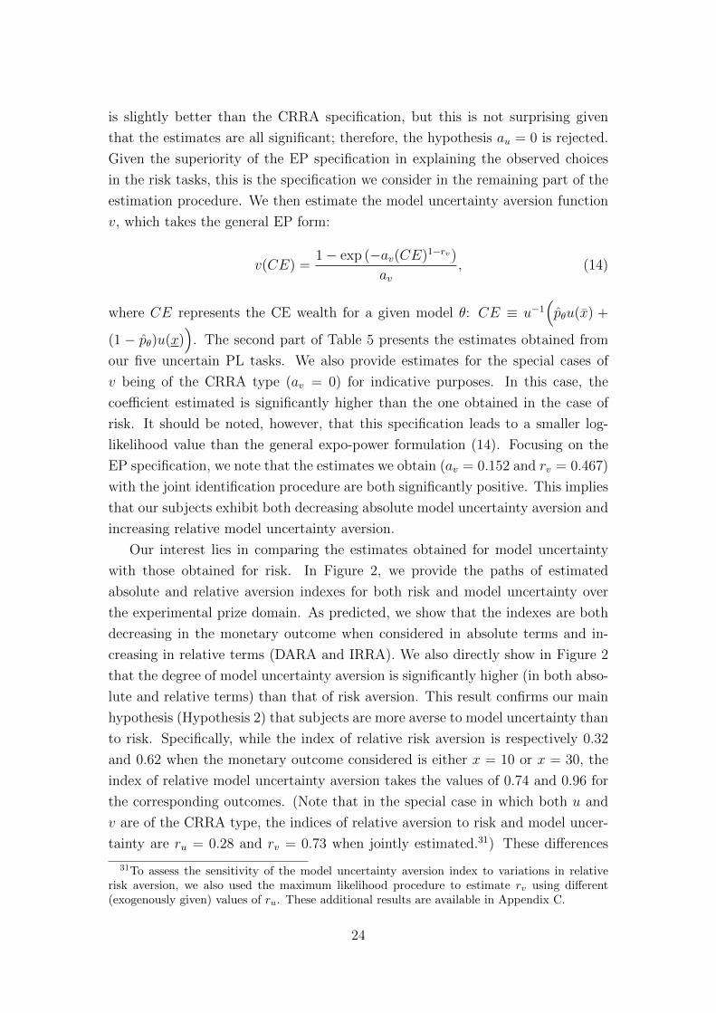
estimation procedure. We then estimate the model uncertainty aversion function
v, which takes the general EP form:
v(CE) =1− exp (−av(CE)1−rv)
av, (14)
where CE represents the CE wealth for a given model θ: CE ≡ u−1(pθu(x) +
(1 − pθ)u(x))
. The second part of Table 5 presents the estimates obtained from
our five uncertain PL tasks. We also provide estimates for the special cases of
v being of the CRRA type (av = 0) for indicative purposes. In this case, the
coefficient estimated is significantly higher than the one obtained in the case of
risk. It should be noted, however, that this specification leads to a smaller log-
likelihood value than the general expo-power formulation (14). Focusing on the
EP specification, we note that the estimates we obtain (av = 0.152 and rv = 0.467)
with the joint identification procedure are both significantly positive. This implies
that our subjects exhibit both decreasing absolute model uncertainty aversion and
increasing relative model uncertainty aversion.
Our interest lies in comparing the estimates obtained for model uncertainty
with those obtained for risk. In Figure 2, we provide the paths of estimated
absolute and relative aversion indexes for both risk and model uncertainty over
the experimental prize domain. As predicted, we show that the indexes are both
decreasing in the monetary outcome when considered in absolute terms and in-
creasing in relative terms (DARA and IRRA). We also directly show in Figure 2
that the degree of model uncertainty aversion is significantly higher (in both abso-
lute and relative terms) than that of risk aversion. This result confirms our main
hypothesis (Hypothesis 2) that subjects are more averse to model uncertainty than
to risk. Specifically, while the index of relative risk aversion is respectively 0.32
and 0.62 when the monetary outcome considered is either x = 10 or x = 30, the
index of relative model uncertainty aversion takes the values of 0.74 and 0.96 for
the corresponding outcomes. (Note that in the special case in which both u and
v are of the CRRA type, the indices of relative aversion to risk and model uncer-
tainty are ru = 0.28 and rv = 0.73 when jointly estimated.31) These differences
31To assess the sensitivity of the model uncertainty aversion index to variations in relativerisk aversion, we also used the maximum likelihood procedure to estimate rv using different(exogenously given) values of ru. These additional results are available in Appendix C.
24

Figure 2: Absolute (left) and relative (right) risk and model uncertainty aversionusing EP estimates (95% confidence in gray).
0
.2
.4
.6
.8
1
Absolu
te a
vers
ion
0 5 10 15 20 25 30 35Monetary outcome (euros)
model uncertainty
risk
0
.5
1
1.5
Rela
tive a
vers
ion
0 5 10 15 20 25 30 35Monetary outcome (euros)
model uncertainty
risk
between the attitudes toward objective and subjective probabilities now enable us
to quantify the attitude subjects manifest toward ambiguity.
4.2.4 The implications for ambiguity attitude
The joint characterization of functions u and v representing the subjects’ atti-
tudes toward the different types of uncertainty has an important direct implication
for ambiguity aversion. Using the identity φ ≡ v ◦ u−1 and the results obtained in
the previous section, we now characterize directly the attitude subjects manifest
toward ambiguity and compute the parameters of absolute and relative ambigu-
ity aversion (see Appendix A for the detailed analytical computations under the
double EP specification). Figure 3 illustrates these parameters. While we observe
Figure 3: Absolute (left) and relative (right) ambiguity aversion obtained with EPfunction estimates
0
.2
.4
.6
.8
1
Absolu
te A
mbig
uity A
vers
ion
0 2 4 6 8 10 12 14 16Expected Utility levels
0
.5
1
1.5
Rela
tive A
mbig
uity A
vers
ion
0 2 4 6 8 10 12 14 16Expected Utility levels
a clearly decreasing trend in the degree of absolute ambiguity aversion, the degree
25

of relative ambiguity aversion is fairly constant over the domain considered. As
previously mentioned, however, the domain of the ambiguity function φ is not the
same monetary outcome domain as that of u and v. Instead, φ is defined over
expected utility levels U . In this sense, the vertical dashed lines in Figure 3 rep-
resent the levels of utility obtained for the corresponding monetary outcomes in
Figure 2, when the utility function u is of the EP type and coefficients are those
reported in Table 5.
To assess the robustness of the CRAA result featured in Figure 3, we apply
the joint estimation procedure directly to u and φ (both of which are of the EP
type). In other words, we let the ambiguity aversion function be:
φ(U) =1− exp (−aφ(U)1−rφ)
aφ, (15)
where U represents the expected utility obtained under a given model θ (i.e. U ≡pθu(o) + (1− pθ)u(o)) and u is defined as in equation (13). The estimated results
are in the last two columns of Table 5. In this case, the coefficient aφ of the EP
formulation is not significant at the 5% level (p − value = 0.062). The function
describing preferences for ambiguity is therefore instead better represented by
a CRAA function. Under this particular specification, we estimate the CRAA
parameter to be 0.53. It does not perfectly match the value shown in Figure 3,
but this should not be surprising given that the ambiguity functions do not share
the same specifications in the two cases. If we instead consider the case of u being
CRRA, we also obtain a non-significant coefficient aφ (p − value = 0.093) under
the EP specification and estimate the coefficient rφ = 0.62 under CRAA.32
5 Conclusion
Uncertainty is pervasive in both collective and individual decision-making pro-
cesses. The past few years have witnessed a wealth of studies encompassing mul-
tiple academic fields aiming to better formalize the decision process in the face
of uncertainty. This body of research investigates, through the development of
theoretical frameworks tested through experimental analyses, how individuals in-
tegrate available information in the process of decision-making. In particular,
scholars have developed multiple decision models to account for attitudes toward
ambiguity. They have also adopted these models to explain individuals’ behavior
32In this case, we could have obtained the result directly from the twofold CRRA estimationresults provided in Appendix A, given that φ is of the CRAA type with rφ = rv−ru
1−ru , when bothu and v are CRRA (Berger et al., 2017).
26

in multiple contexts and increasingly applied them to prescribe optimal strategies
in the face of uncertainty.
The growing application of ambiguity aversion models calls for the develop-
ment of experimental efforts enabling a better understanding of the underlying
mechanisms at play and a more precise quantification of ambiguity preferences,
similar to what has been done in the study of risk. In this paper, we provide new
experimental evidence on ambiguity attitudes by means of attitudes toward model
uncertainty and risk. In particular, our design enables us to disentangle the role
of aleatory and epistemic uncertainty in determining individuals’ ambiguity atti-
tudes. We can then quantify, through a joint elicitation procedure, the extent to
which ambiguity aversion exists as well as the properties of the ambiguity aversion
function in the context of the smooth model.
Two main findings emerge from our analysis. First, we show that subjects
tend to be both risk and model uncertainty averse, though they exhibit stronger
aversion to model uncertainty than to risk. Following the smooth ambiguity model
of choice under uncertainty, we interpret this behavioral characteristic as evidence
of ambiguity aversion. Using a joint estimation procedure, we elicit the degree
of ambiguity aversion, which we estimate to be twice as large as the degree of
risk aversion when considered in relative terms. Second, investigating in more
detail attitude toward model uncertainty, we find that model uncertainty aversion
is decreasing in wealth when considered in absolute terms and increasing when
considered in relative terms. Regarding ambiguity attitude, we find evidence of
DAAA and CRAA. These results have several implications for decisions involving
aspects of insurance, self-insurance and self-protection in multi-period contexts.
Indeed, recent theoretical developments suggest that exhibiting DAAA in the pres-
ence of ambiguity will lead to (1) an increase in the insurance coverage rate, (2)
raise the optimal level of SI, and (3) favor a higher optimal level of SP (if the
degree of disagreement among models is not increasing in the level of effort).
It should, however, be noted that the estimated preferences and parameters
we obtained in the context of our experiment may not have predictive power for
behavior outside a controlled laboratory environment. Our experimental results
should thus be primarily understood as identifying differences between risk and
model uncertainty, as well as testing behavioral hypotheses whose relevance may
only be fully appreciated within a particular economic framework. Further inves-
tigation of individual behaviors in the face of model uncertainty and ambiguity in
real-world decisions is therefore warranted.
27

Appendix
A Absolute and relative ambiguity aversion
When the functions characterizing risk and model uncertainty preferences are
both of the expo-power type and are respectively defined as u(x) = 1−exp(−aux1−ru )au
and v(x) = 1−exp(−avx1−rv )av
, we can write the ambiguity function φ ≡ v ◦ u−1:
φ(U) =1− exp
(− av
(− ln(1−auU)
au
) 1−rv1−ru
)av
,
where U belongs to the space of expected utilities. In this case, we can show that
the Arrow-Pratt absolute ambiguity aversion index is:
−φ′′(U)
φ′(U)=av(1−rv1−ru
)(− ln(1−auU)au
) ru−rv1−ru
+(
auln(1−auU)
)ru−rv1−ru − au
1− auU. (A.1)
We can then easily show that in the special case in which u and v are both of the
CARA type (i.e. when ru = rv = 0), this index collapses to:
−φ′′(U)
φ′(U)=
av − au1− auU
. (A.2)
This index is positive whenever av > au, so that absolute ambiguity aversion re-
sults from higher absolute model uncertainty aversion than absolute risk aversion.
Similarly, in the special case in which u and v are both of the CRRA type (i.e.
when au = av = 0), the absolute ambiguity aversion becomes:
−φ′′(U)
φ′(U)=
rv − ru(1− ru)U
, (A.3)
and is positive whenever rv > ru.
B Robust estimates of risk and model uncer-
tainty preferences
As each of our subjects provided multiple choices in the experiment, we may
want to correct for the possible correlation of errors associated with a given sub-
ject (which may for example be due to unobserved individual effects). In this
28
case, we treat the residuals from the same subject as potentially correlated and
make the correction when calculating standard errors of estimates. As Andersen
et al. (2008) argued, this procedure allows heteroskedasticity between and within
clusters, as well as autocorrelation within clusters, and generalizes the “robust
standard errors” approach popular in econometrics. The estimates of risk and
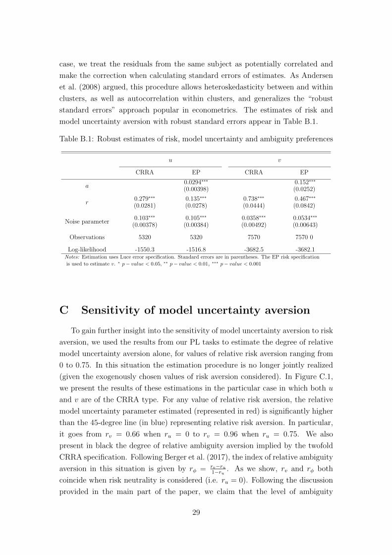
model uncertainty aversion with robust standard errors appear in Table B.1.
Table B.1: Robust estimates of risk, model uncertainty and ambiguity preferences
u v
CRRA EP CRRA EP
a0.0294∗∗∗ 0.152∗∗∗
(0.00398) (0.0252)
r0.279∗∗∗ 0.135∗∗∗ 0.738∗∗∗ 0.467∗∗∗
(0.0281) (0.0278) (0.0444) (0.0842)
Noise parameter0.103∗∗∗ 0.105∗∗∗ 0.0358∗∗∗ 0.0534∗∗∗
(0.00378) (0.00384) (0.00492) (0.00643)
Observations 5320 5320 7570 7570 0
Log-likelihood -1550.3 -1516.8 -3682.5 -3682.1Notes: Estimation uses Luce error specification. Standard errors are in parentheses. The EP risk specification
is used to estimate v. ∗ p− value < 0.05, ∗∗ p− value < 0.01, ∗∗∗ p− value < 0.001
C Sensitivity of model uncertainty aversion
To gain further insight into the sensitivity of model uncertainty aversion to risk
aversion, we used the results from our PL tasks to estimate the degree of relative
model uncertainty aversion alone, for values of relative risk aversion ranging from
0 to 0.75. In this situation the estimation procedure is no longer jointly realized
(given the exogenously chosen values of risk aversion considered). In Figure C.1,
we present the results of these estimations in the particular case in which both u
and v are of the CRRA type. For any value of relative risk aversion, the relative
model uncertainty parameter estimated (represented in red) is significantly higher
than the 45-degree line (in blue) representing relative risk aversion. In particular,
it goes from rv = 0.66 when ru = 0 to rv = 0.96 when ru = 0.75. We also
present in black the degree of relative ambiguity aversion implied by the twofold
CRRA specification. Following Berger et al. (2017), the index of relative ambiguity
aversion in this situation is given by rφ = rv−ru1−ru . As we show, rv and rφ both
coincide when risk neutrality is considered (i.e. ru = 0). Following the discussion
provided in the main part of the paper, we claim that the level of ambiguity
29
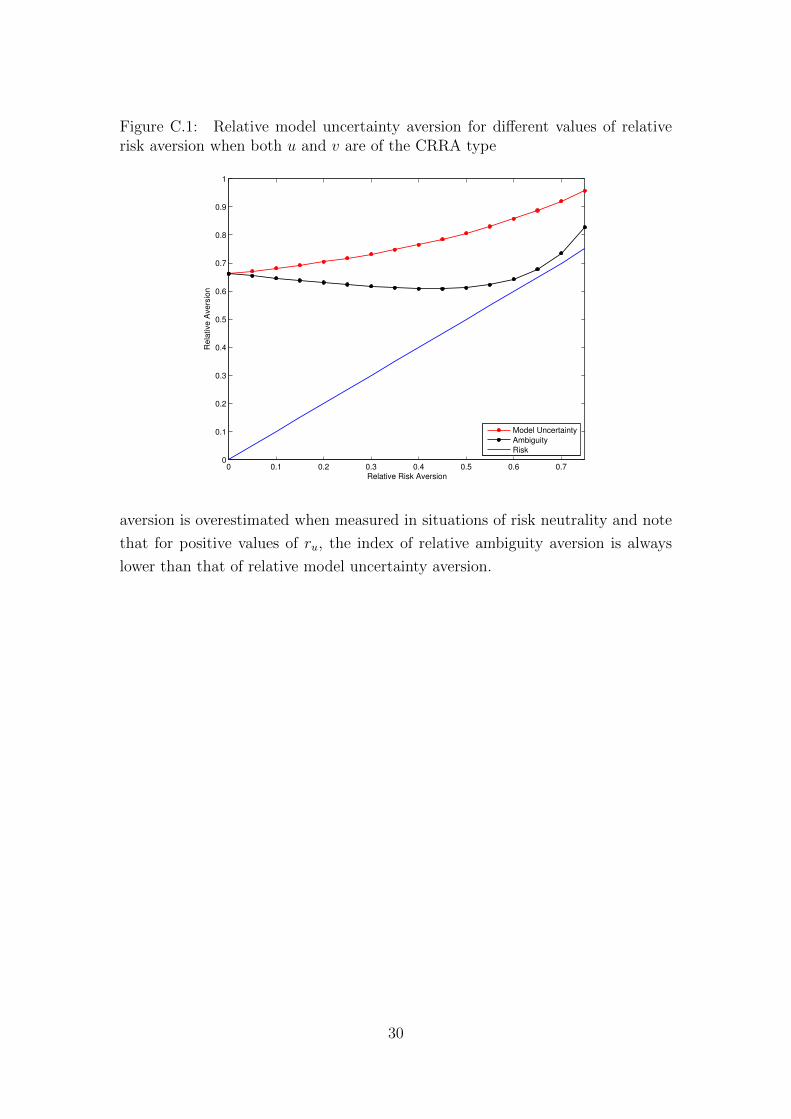
Figure C.1: Relative model uncertainty aversion for different values of relativerisk aversion when both u and v are of the CRRA type
0 0.1 0.2 0.3 0.4 0.5 0.6 0.70
0.1
0.2
0.3
0.4
0.5
0.6
0.7
0.8
0.9
1
Relative Risk Aversion
Re
lative A
vers
ion
Model Uncertainty
Ambiguity
Risk
aversion is overestimated when measured in situations of risk neutrality and note
that for positive values of ru, the index of relative ambiguity aversion is always
lower than that of relative model uncertainty aversion.
30

References
Abdellaoui, M., A. Baillon, L. Placido, and P. P. Wakker (2011). The rich domainof uncertainty: Source functions and their experimental implementation. TheAmerican Economic Review 101 (2), 695–723.
Abdellaoui, M., C. Barrios, and P. P. Wakker (2007). Reconciling introspectiveutility with revealed preference: Experimental arguments based on prospecttheory. Journal of Econometrics 138 (1), 356–378.
Adair, J. G., T. W. Dushenko, and R. Lindsay (1985). Ethical regulations andtheir impact on research practice. American Psychologist 40 (1), 59.
Ahn, D., S. Choi, D. Gale, and S. Kariv (2014). Estimating ambiguity aversion ina portfolio choice experiment. Quantitative Economics 5 (2), 195–223.
Alary, D., C. Gollier, and N. Treich (2013). The effect of ambiguity aversion oninsurance and self-protection. The Economic Journal 123 (573), 1188–1202.
Andersen, S., G. W. Harrison, M. I. Lau, and E. E. Rutstrom (2006). Elicitationusing multiple price list formats. Experimental Economics 9 (4), 383–405.
Andersen, S., G. W. Harrison, M. I. Lau, and E. E. Rutstrom (2008). Elicitingrisk and time preferences. Econometrica 76 (3), 583–618.
Attanasio, O., J. Banks, and S. Tanner (2002, Aug). Asset holding and consump-tion volatility. Journal of Political Economy 110, 771–792.
Aydogan, I., L. Berger, V. Bosetti, and N. Liu (2018). Three layers of uncertaintyand the role of model misspecification: an experiment. IGIER Working Paper623, Bocconi University.
Baillon, A. and L. Placido (2019). Testing constant absolute and relative ambiguityaversion. Journal of Economic Theory .
Berger, L. (2014). Precautionary saving and the notion of ambiguity prudence.Economics Letters 123 (2), 248 – 251.
Berger, L. (2016). The impact of ambiguity and prudence on prevention decisions.Theory and Decision 80 (3), 389–409.
Berger, L. (2019). A randomness device to create the conditions of ignorance inthe lab. mimeo.
Berger, L. and V. Bosetti (2019). Are policymakers ambiguity averse? TheEconomic Journal .
Berger, L., J. Emmerling, and M. Tavoni (2017). Managing catastrophic climaterisks under model uncertainty aversion. Management Science 63 (3), 749–765.
Brunnermeier, M. K. and S. Nagel (2008). Do wealth fluctuations generate time-varying risk aversion? micro-evidence on individuals? asset allocation (digestsummary). American Economic Review 98 (3), 713–736.
Budescu, D. V., A. K. Rantilla, H.-T. Yu, and T. M. Karelitz (2003). The effects ofasymmetry among advisors on the aggregation of their opinions. OrganizationalBehavior and Human Decision Processes 90 (1), 178–194.
Cabantous, L. (2007). Ambiguity aversion in the field of insurance: Insurers?attitude to imprecise and conflicting probability estimates. Theory and Deci-sion 62 (3), 219–240.
Cabantous, L., D. Hilton, H. Kunreuther, and E. Michel-Kerjan (2011). Is im-
31
precise knowledge better than conflicting expertise? evidence from insurers?decisions in the united states. Journal of Risk and Uncertainty 42 (3), 211–232.
Cerreia-Vioglio, S., F. Maccheroni, M. Marinacci, and L. Montrucchio (2013).Classical subjective expected utility. Proceedings of the National Academy ofSciences 110 (17), 6754–6759.
Charness, G., U. Gneezy, and A. Imas (2013). Experimental methods: Elicitingrisk preferences. Journal of Economic Behavior & Organization 87, 43–51.
Chetty, R. (2006). A New Method of Estimating Risk Aversion. American Eco-nomic Review 96 (5), 1821–1834.
Chew, S. H., B. Miao, and S. Zhong (2017). Partial ambiguity. Economet-rica 85 (4), 1239–1260.
Chiappori, P.-A. and M. Paiella (2011). Relative risk aversion is constant: Ev-idence from panel data. Journal of the European Economic Association 9 (6),1021–1052.
Davis, D. D. and C. A. Holt (1993). Experimental economics. Princeton universitypress.
Dimmock, S. G., R. Kouwenberg, and P. P. Wakker (2016). Ambiguity attitudesin a large representative sample. Management Science 62 (5), 1363–1380.
Dionne, G. and L. Eeckhoudt (1985). Self-insurance, self-protection and increasedrisk aversion. Economics Letters 17 (1-2), 39–42.
Eeckhoudt, L. and C. Gollier (2005). The impact of prudence on optimal preven-tion. Economic Theory 26 (4), 989–994.
Ehrlich, I. and G. Becker (1972). Market insurance, self-insurance, and self-protection. The Journal of Political Economy 80 (4), 623–648.
Ellsberg, D. (1961). Risk, ambiguity, and the Savage axioms. The QuarterlyJournal of Economics 75, 643–669.
Epstein, L. G. and Y. Halevy (2018). Ambiguous correlation. The Review ofEconomic Studies .
Fischbacher, U. (2007). z-tree: Zurich toolbox for ready-made economic experi-ments. Experimental economics 10 (2), 171–178.
Gajdos, T. and J.-C. Vergnaud (2013). Decisions with conflicting and impreciseinformation. Social Choice and Welfare 41 (2), 427–452.
Ghirardato, P. (2004). Defining ambiguity and ambiguity attitude. Uncertaintyin economic theory: A collection of essays in honor of David Schmeidler’s 65thbirthday , 36–45.
Gierlinger, J. and C. Gollier (2008, November). Socially efficient discounting underambiguity aversion. Technical Report 561, IDEI, Toulouse, Toulouse.
Gilboa, I. and M. Marinacci (2013). Ambiguity and the bayesian paradigm. InAdvances in Economics and Econometrics: Theory and Applications, TenthWorld Congress of the Econometric Society. D. Acemoglu, M. Arellano, and E.Dekel (Eds.). New York: Cambridge University Press.
Gilboa, I. and D. Schmeidler (1989). Maxmin expected utility with a non-uniqueprior. Journal of Mathematical Economics 18 (2), 141–154.
Grant, S. and B. Polak (2013). Mean-dispersion preferences and constant absolute
32

uncertainty aversion. Journal of Economic Theory 148 (4), 1361–1398.
Guerdjikova, A. and E. Sciubba (2015). Survival with ambiguity. Journal ofEconomic Theory 155, 50–94.
Hansen, L. P. (2014). Nobel lecture: Uncertainty outside and inside economicmodels. Journal of Political Economy 122 (5), 945–987.
Hansen, L. P. and M. Marinacci (2016). Ambiguity aversion and model misspeci-fication: An economic perspective. Statistical Science 31, 511–515.
Hansen, L. P. and T. J. Sargent (2001). Robust control and model uncertainty.American Economic Review 91 (2), 60–66.
Hardy, G. H., E. M. Wright, D. R. Heath-Brown, and J. H. Silverman (1979). Anintroduction to the theory of numbers, Volume 4. Clarendon press Oxford.
Harrison, G. W., M. I. Lau, and E. E. Rutstrom (2007). Estimating risk at-titudes in Denmark: A field experiment. The Scandinavian Journal of Eco-nomics 109 (2), 341–368.
Harrison, G. W. and E. E. Rutstrom (2008). Risk aversion in the laboratory. InJ. C. Cox and G. W. Harrison (Eds.), Risk Aversion in Experiments (Research inExperimental Economics, Volume 12), Chapter 6, pp. 41–196. Emerald GroupPublishing Limited.
Heal, G. and A. Millner (2014). Reflections: Uncertainty and decision makingin climate change economics. Review of Environmental Economics and Pol-icy 8 (1), 120–137.
Hertwig, R. and A. Ortmann (2008). Deception in experiments: Revisiting thearguments in its defense. Ethics & Behavior 18 (1), 59–92.
Holt, C. A. and S. K. Laury (2002). Risk aversion and incentive effects. Americaneconomic review 92 (5), 1644–1655.
Holt, C. A. and S. K. Laury (2005). Risk aversion and incentive effects: New datawithout order effects. American Economic Review , 902–904.
IPCC (2014a). Climate Change 2014: Impacts, Adaptation, and Vulnerability.Part A: Global and Sectoral Aspects. Contribution of Working Group II to theFifth Assessment Report of the Intergovernmental Panel on Climate Change.[Field, CB and Barros, VR and Dokken, DJ and Mach, KJ and Mastrandrea,MD and Bilir, TE and Chatterjee, M and Ebi, KL and Estrada, YO and Genova,RC and others]. Cambridge, UK/New York, NY: Cambridge University Press.
IPCC (2014b). Climate Change 2014, Mitigation of Climate Change. Contributionof Working Group III to the Fifth Assessment Report of the IntergovernmentalPanel on Climate Change. Summary for Policymakers. Working Group IIIto the Fifth Assessment Report of the Intergovernmental Panel on ClimateChange [Edenhofer, O., R. Pichs-Madruga, Y. Sokona, E. Farahani, S. Kadner,K. Seyboth, A. Adler, I. Baum, S. Brunner, P. Eickemeier, B. Kriemann, J.Savolainen, S. Schlomer, C. von Stechow, T. Zwickel and J.C. Minx (eds.)].Cambridge University Press, Cambridge, United Kingdom and New York, NY,USA.
Jullien, B., B. Salanie, and F. Salanie (1999, June). Should more risk-averse agentsexert more effort? The Geneva Risk and Insurance Review 24 (1), 19–28.
Klibanoff, P., M. Marinacci, and S. Mukerji (2005). A smooth model of decision
33

making under ambiguity. Econometrica 73, 1849–1892.
Krawczyk, M. et al. (2013). Delineating deception in experimental economics:Researchers? and subjects? views. Faculty of Economic Sciences WorkingPaper, University of Warsaw .
Kriegler, E., J. W. Hall, H. Held, R. Dawson, and H. J. Schellnhuber (2009).Imprecise probability assessment of tipping points in the climate system. Pro-ceedings of the National Academy of Sciences 106 (13), 5041–5046.
Lenton, T. M., H. Held, E. Kriegler, J. W. Hall, W. Lucht, S. Rahmstorf, andH. J. Schellnhuber (2008). Tipping elements in the earth’s climate system.Proceedings of the National Academy of Sciences 105 (6), 1786–1793.
Luce, R. D. (1959). Individual choice behavior. New York: Wiley.
Maccheroni, F., M. Marinacci, and A. Rustichini (2006). Ambiguity aversion, ro-bustness, and the variational representation of preferences. Econometrica 74 (6),1447–1498.
Marinacci, M. (2015). Model uncertainty. Journal of the European EconomicAssociation 13 (6), 1022–1100.
Menges, R. J. (1973). Openness and honesty versus coercion and deception inpsychological research. American Psychologist 28 (12), 1030.
Saha, A. (1993). Expo-power utility: A ”flexible” form for absolute and relativerisk aversion. American Journal of Agricultural Economics 75 (4), 905–913.
Savage, L. (1954). The Foundations of Statistics. New York: J. Wiley. secondrevised edition, 1972.
Snow, A. (2011). Ambiguity aversion and the propensities for self-insurance andself-protection. Journal of Risk and Uncertainty 42, 27–43.
von Neumann, J. and O. Morgenstern (1944). Theory of Games and EconomicBehavior. Princeton University Press.
Wald, A. (1950). Statistical decision functions. New York: John Wiley & Sons.
34