characterization of the modal characteristics of

1 This material is declared a work of the U.S. Government and is not subject to copyright protection in the United States. Approved for

public release; distribution is unlimited.

Proceedings of the ASME Turbo Expo 2017

GT2017

June 26-30, 2017, Charlotte, NC, USA

GT2017-63633

CHARACTERIZATION OF THE MODAL CHARACTERISTICS OF STRUCTURES

OPERATING IN DENSE LIQUID TURBOPUMPS

Joseph Chiu City College of New York

New York, New York

Andrew M. Brown NASA/Marshall Space Flight Center

Huntsville, Al 35812

ABSTRACT It is well-known that the natural frequencies of structures

immersed in heavy liquids will decrease due to the fluid

“added-mass” effect. This reduction has not been precisely

determined, though, with indications that it is in the 20-40%

range for water. In contrast, the mode shapes of these

structures have always been assumed to be invariant in liquids.

Recent modal testing at NASA/Marshall Space Flight Center of

turbomachinery inducer blades in liquid oxygen, which has a

density slightly greater than water, indicates that the mode

shapes change appreciably, though. This paper presents a

study that examines and quantifies the change in mode shapes

as well as more accurately defines the natural frequency

reduction. A literature survey was initially conducted and test-

verified analytical solutions for the natural frequency

reductions were found for simple geometries, including a

rectangular plate and an annular disk. The ANSYS©

fluid/structure coupling methodology was then applied to

obtain numerical solutions, which compared favorably with the

published results. This initial study indicated that mode shape

changes only occur for non-symmetric boundary conditions.

Techniques learned from this analysis were then applied to the

more complex inducer model. ANSYS numerical results for

both natural frequency and mode shape compared well with

modal test in air and water. A number of parametric studies

were also performed to examine the effect of fluid density on

the structural modes, reflecting the differing propellants used in

rocket engine turbomachinery. Some important findings were

that the numerical order of mode shapes changes with density

initially, and then with higher densities the mode shapes

themselves warp as well. Valuable results from this study

include observations on the causes and types of mode shape

alteration and an improved prediction for natural frequency

reduction in the range of 30-41% for preliminary design.

Increased understanding and accurate prediction of these

modal characteristics is critical for assessing resonant

response, correlating finite element models to modal test, and

performing forced response in turbomachinery.

NOMENCLATURE

IP In Phase

OP Out of Phase

MAC Modal Assurance Criterion

MN Mode Number

MS Mode Shape

LH2 Liquid Hydrogen

LOX Liquid Oxygen

INTRODUCTION During the design of the J2-X rocket engine in 2012,

preliminary analysis of the two inducer blades in the Liquid

Oxygen (LOX) turbopump (Figure 1) predicted high stresses

from a possibly resonant dynamic forcing function. It is well-

known that the natural frequencies of a structure decrease when

it is immersed in a fluid due to the effective added-mass, so a

“knockdown factor”, which is the percentage that the natural

frequencies decrease, was applied to the frequencies in the

Campbell Diagram, but previously-used factors based on

anecdotal experience was tremendously inconsistent, with a

range of between 20 and 40%. A modal test was therefore

performed to find the natural frequencies of the J2-X inducer

blades immersed in water, which has a density slightly greater

than LOX, to enable accurate prediction of resonance and for

the model verification critical for forced response analysis.

The blades were tested in both air and water, and in several

different housing configurations to examine the effects of tip

clearance and grooves in the housing. The results indicated that

in addition to the natural frequency change in water, which was

expected, the modes shapes changed as well. There was no

indication in initial literature surveys or previous experiments

that this would occur, so the result was surprising. These

changes made both correlation with the finite element model

and use of the model for forced response analysis problematic.

An attempt at implementation of a new acoustic/structure finite



element formulation was made, but there were some limitations

in the software at that time preventing complete reliance on that

technique.

Figure 1. J2-X LOX Turbopump Inducer (not to scale)

There has been some research in this field, but the only

research found provides analytical and numerical data on the

“knockdown factor”, without any mention of mode shape

alteration. One of the first studies was by Lindholm [1] in 1965,

which presented experimental results for the natural frequencies

of a cantilever plate in fluid. No mention is made of a change

in the mode shapes, though. Kwak [2] presents an excellent

study with both theoretical and experimental results of an

annual disk, and Askari [3] develops a more extensive theoretical

basis for the frequency reduction for the same geometry.

Kerboua [4] develops exact analytical expressions for the fluid

added-mass for a flat plate in order to develop the frequency

knockdown using some advanced thin-shell theories, but again

does not identify the loss of mode shape consistency. Hosseini-

Hashimi [5] state that the “simplifying hypothesis that the wet

and dry mode shapes are the same, is not assumed in this paper”

in their study of Mindlin plates in a fluid, but do not present any

investigation into or results for the mode shape change.

This change in the mode shapes has motivated the current

study discussed in this paper. The focus is on quantifying the

change in mode shapes, developing a methodology to

accurately predict the changes, and to attempt to learn why the

changes take place. In addition, a more refined quantification

of the natural frequency change is sought. In particular, the

effect of density on the structural modes of the inducer blades is

evaluated for its effect on the modal characteristics.

METHODOLOGY

The general purpose multi-physics/finite element code

ANSYS WorkBench 17.0 with the ACT fluid/structure coupling

extension is the primary numerical tool used in this study to

obtain the modal characteristics of structures immersed in

fluids. To gain an understanding of the fluid/structure coupling

methodology, simpler geometries are first used to verify that the

ANSYS settings accurately represent the physics and that the

modal characteristics match results obtained from analytical

solutions found in the literature. These geometries include a flat

rectangular plate and an annular disk, and are discussed in more

detail in the next section. Afterwards, a parametric study is

performed for the annular disk to identify the effect of fluid

density on its modal characteristics.

After these analyses are completed, the same numerical

techniques and settings can be applied to analyze the inducer

blades. However, since there is no analytical solution, modal

test results are used as a comparison to see if the natural

frequencies from the numerical model are in good agreement

with these test frequencies. If there is a good match on the

modal characteristics, the same parametric study done for the

annular disk can now be performed for the inducer blades.

Observations and conclusions can then be drawn about how

fluid density affects the natural frequencies and mode shapes of

the inducer blades. It is important to note that the analyses were

performed at room temperature, so the temperature effects on

the modal characteristics of the structures are not taken into

account. These effects are ignored to isolate the effect of the

fluid-added mass on the mode shapes.

FLAT PLATE The first of the simple geometries examined is a flat

rectangular plate with one fixed end. The analytical solutions

for the natural frequencies of this configuration in vacuum are

shown in equation (1) below, from Blevins [6]

(1)

where a and h are the length and thickness of the plate,

respectively, i and j are the numbers of half-waves in the mode

shape along its longitudinal and transverse axes, respectively, E

is the modulus of elasticity, v is Poisson’s ratio, is the mass

per unit area, and as a function of a, b, i, and j is a constant

found in Table 11-4 of the Blevin’s text. If the structure is

immersed in fluid, the frequencies are adjusted using equation

(2), also from Blevins

(2)

where is the mass of the plate, and is the “added mass”,

which is a quantification of the fluid that moves with the blade

during its modal deformation. The added mass is a function of

the fluid and mode shape and is tabulated in Table 14-4 of the

Blevins text.



The next step in the process is a numerical analysis. A

solid geometry model is initially created with a geometric

modeling software such as ANSYS DesignModeler© or

SpaceClaim©. A fluid domain is also created using the

“enclosure” feature in SpaceClaim©. A transparent view of the

model is shown in Figure 2.

Figure 2. Transparent View of Cantilever Plate Inside Fluid

Domain

The model is then imported into ANSYS Mechanical and a

modal analysis is performed. The properties of the plate and the

fluid domain are listed in Table 1.

Table 1. Properties for Rectangular Plate Analysis

Plate Fluid Domain

Length=46.736 cm (18 in) Length =68.58cm (27 in)

Width=30.48 cm (12 in) Width =53.34 cm (21 in)

Thickness = 0.127 cm (0.05

in)

Height =23.0 cm (9.05in)

Density: 8193 kg/m3 (7.67e-

4 slinch/in3)

Density =1.06e-5 kg/m3

(9.36 x 10-5 slinch/in3)

E (Young’s Modulus) =

206.84 GPa (3e7 psi)

c (Speed of sound)=148e3

cm/s (58346.46 in/s)

(Poisson’s Ratio) = 0.27

ANSYS [7] advises using a fluid domain that is at least half the

size wavelength of the fluid as determined in equation (3)

(3)

where is the wavelength of the fluid, c is the speed of sound,

and f is the highest natural frequency of interest. Setting this

size is important, as the modes of the coupled

acoustic/structural system are highly dependent upon it, and the

goal is to avoid acoustic modes if structure-only modes are

being sought. However, too large of a domain will make the

solution computationally intensive, so some iteration is required

to establish convergence without too much expense.

Convergence in this case was reached with the dimensions as

shown, which are only about half of the recommended size for

water.

If it is known a-priori that coupled acoustic-structure

modes are not of interest, then the speed of sound can be set to

a very high value, or equivalently, an “incompressible” flag in

the software can be set to move the acoustic modes well out of

the range of the structural modes while maintaining the mass-

added effect of the fluid. Of course, this uncoupled assumption

must be carefully made, as studies have shown significant and

unanticipated effects of structural-acoustic coupling in

turbomachinery, particularly in LH2 [8].

The next step is to perform the pre-processing for the finite

element model of the fluid and structure. A high-density

tetrahedral mesh option is used for the fluid elements, and

three-element thick hexagonal elements are used for the plate.

For the fluid and the structural domains to be coupled

successfully, the nodes of the plate must be coincident with

nodes of the fluid, as shown in Figure 3. The acoustic body

condition is then specified for the fluid domain, enabling the

application of fluid elements, and the fluid/structure interface is

identified at all the faces of the plate.

Figure 3. Coincident Nodes at Fluid/Structure Interface

At this point the modal characteristics of the cantilever

plate can be obtained. Two analyses are performed to compare

the natural frequencies and mode shapes in vacuum and then in

water. We use Blevin’s categorization scheme in which each

mode shape is identified by the number of half waves along the

length followed by the number of half waves along the width,

e.g., mode 1,3 has one length-wise half wave and three width-

wise half waves. To enable a consistent relationship between the

modal characteristics and fluid density independent of the use

of the acoustic fluid/structure formulation, the vacuum case was

always performed using fluid elements with a negligible density.

The natural frequencies found using the analytical solution are

in good agreement with the natural frequencies found using the

numerical model for this vacuum case; five of the first six

natural frequencies have relative error percentages less than 1%

and the sixth is under 1.5%. On the other hand, most of the

natural frequency values for water had relative errors between

the numerical and analytical results of well over 10%, as shown

in Table 2.

Table 2. Nat. Frequency Comparison, Water

Mode Shape 1,1 1,2 2,1 2,2 1,3 3,1

analytical nat.

freq’s (hz)

1.03 5.48 6.43 18.54 27.09 18.4

3

FEA nat. freq’s

(hz)

1.24 5.85 8.82 20.86 31.74 28.2

8

relative error

(%)

20.5 6.7 37.3 12.6 17.1 53.4

Upon close examination, it appears that the mode shapes

themselves change when submerged in water, as shown by



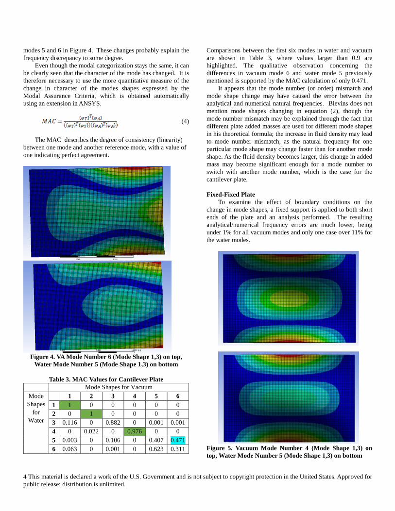
modes 5 and 6 in Figure 4. These changes probably explain the

frequency discrepancy to some degree.

Even though the modal categorization stays the same, it can

be clearly seen that the character of the mode has changed. It is

therefore necessary to use the more quantitative measure of the

change in character of the modes shapes expressed by the

Modal Assurance Criteria, which is obtained automatically

using an extension in ANSYS.

(4)

The MAC describes the degree of consistency (linearity)

between one mode and another reference mode, with a value of

one indicating perfect agreement.

Figure 4. VA Mode Number 6 (Mode Shape 1,3) on top,

Water Mode Number 5 (Mode Shape 1,3) on bottom

Table 3. MAC Values for Cantilever Plate

Mode Shapes for Vacuum

Mode

Shapes

for

Water

1 2 3 4 5 6

1 1 0 0 0 0 0

2 0 1 0 0 0 0

3 0.116 0 0.882 0 0.001 0.001

4 0 0.022 0 0.976 0 0

5 0.003 0 0.106 0 0.407 0.471

6 0.063 0 0.001 0 0.623 0.311

Comparisons between the first six modes in water and vacuum

are shown in Table 3, where values larger than 0.9 are

highlighted. The qualitative observation concerning the

differences in vacuum mode 6 and water mode 5 previously

mentioned is supported by the MAC calculation of only 0.471.

It appears that the mode number (or order) mismatch and

mode shape change may have caused the error between the

analytical and numerical natural frequencies. Blevins does not

mention mode shapes changing in equation (2), though the

mode number mismatch may be explained through the fact that

different plate added masses are used for different mode shapes

in his theoretical formula; the increase in fluid density may lead

to mode number mismatch, as the natural frequency for one

particular mode shape may change faster than for another mode

shape. As the fluid density becomes larger, this change in added

mass may become significant enough for a mode number to

switch with another mode number, which is the case for the

cantilever plate.

Fixed-Fixed Plate

To examine the effect of boundary conditions on the

change in mode shapes, a fixed support is applied to both short

ends of the plate and an analysis performed. The resulting

analytical/numerical frequency errors are much lower, being

under 1% for all vacuum modes and only one case over 11% for

the water modes.

Figure 5. Vacuum Mode Number 4 (Mode Shape 1,3) on

top, Water Mode Number 5 (Mode Shape 1,3) on bottom



The modal results show mainly mode number mismatches, with

no changes in the essential modes shapes, although there is a

small change in the relative magnitudes of the mode shapes, as

shown in Figure 5. This can be attributed to the different rates

that the added mass increases by depending on the mode shape,

which is the same case for the cantilever plate.

MAC results also clearly show this result, with qualitatively

well-matching mode pairs yielding values very close to one, but

these numbers not always being on the diagonal, indicating the

modal number mismatch. Comparing these results with those

from the cantilever plate, it appears that symmetry plays a role

in whether the mode shapes change or not, as the mode shapes

change for a non-symmetric cantilever plate but do not for the

symmetric fixed-fixed plate.

ANNULAR DISK An examination is now performed based upon the work by

Kwak described previously. He develops the following

equation for this geometry submerged in a liquid:

, 1

a ww

p

f af

h

(5)

where is the natural frequency in water, is the natural

frequency in air, is the Nondimensionalized Added Virtual

Mass Incremental (NAVMI) factor, is the thickness correction

factor, is the density of water, is the mass density of the

disk, is the outer radius of the disk, and is the thickness of

the disk. An experiment is also presented in the paper for a

steel disk of 200 mm outer diameter, 60 mm inner diameter, and

1.5 mm thick, immersed in a cylindrical tank of water with a

diameter of 500 mm by 180 mm high, with the annular disk 80

mm below the free surface of the water. The disk is placed on a

compliant suspension such that the first disk mode is enough

above the suspension mode to simulate a free-free boundary

condition. The test is used to generate the NAVMI factors;

Figure 6 (from Kwak) plots these for the plate resting on the

surface of the liquid, where (ratio of inner radius to outer

Figure 6. NAVMI factors versus ; (s, n) = (0,1), (0,2)

radius), s is the number of nodal diameters, and n is number of

nodal circles. These values are multiplied by 2.0 for full

immersion in the liquid. Similar charts are presented for (s, n)=

(1,1), (2,1), and (s,n)=(2,0), (3,0).

A numerical analysis is now performed for the annular disk

using the same process as that followed for the rectangular

plate. The properties used for the disk are the same as used by

Kwak. The results agree well with the theoretical values using

Kwak’s equation, as the relative error is less than 3% for both a

semi-infinite theoretical boundary case and the experimental

cases for all mode shapes. This agreement helps to validate the

numerical analytical procedure.

A parametric study is then undertaken to see the effect of

density on the modal characteristics of the annular disk. In

addition to air and water, typical rocket engine fluid media such

as LH2, kerosene, and LOX are used to get a wide range of

fluid densities. The results of this study are shown in Figure 7,

where the mode shapes are identified by their number of nodal

diameters (ND) and nodal circles (NC), and the marks on the

curves correspond to the density of the previously mentioned

propellants, respectively.

The results show that the modal order is generally not

mismatched (i.e., the curves do not intersect), although there are

two exceptions, the 3 ND, 1 NC mode shape and the 0 ND, 2

NC mode shape. These results support the hypothesis that

mode number switching is dependent on the symmetry of the

structure and its boundary conditions, since this case is

completely symmetric.

LOX PUMP INDUCER As the inducer is a complicated geometry, no analytical

solution for the modal characteristics in fluid exists. However,

the numerical modeling procedures developed and verified

using the simpler geometries can be applied, and the results

compared with modal testing in both air and water. The basic

material properties of the blade are a density of 8193 kg/m3,

Young’s Modulus of 202.71 Gpa, and Poisson’s Ratio of 0.29.

The fluid domain is defined to match the cylindrical enclosure

used for the immersed modal test (Figure 8), which has a 19.53

cm diameter and 24.769 cm height. The structural mesh was

generated using a CAD model with a number of detailed

features inside the hub (not in contact with the fluid) removed

to reduce the model size, a high mesh density used for the

inducer blades, and the base of the inducer hub fixed (see

Figure 9). The fluid/structure interface surfaces were specified

at all inducer/hub locations except for the fixed hub surface.

As a first step, a modal analysis in vacuum is now

performed and the results compared with the modal test in air.

For the first 18 modes up to 2900 Hz, the error is less than 2%

and only two of the frequencies have an error of more than 5%,

suggesting that the model is accurate. Next, a modal analysis in

water is performed and compared with the analogous modal

test. Numerous problems had to be overcome to achieve

reproducible results in this submerged modal test, including air



Figure 7. Annular Disk Natural Frequency vs. Immersed Fluid Density

Figure 8. Setup of immersed modal test

Figure 9. Cross-section of inducer solid mesh and

surrounding fluid domain

bubbles and accessibility of the laser measurement system to the

blades. These will tend to increase the error. Because of the

limited access issue, only the frequencies from the test were

obtained, and these are compared with the analytical

frequencies in in Table 4. These results show excellent

agreement, with the first 7 modes having an error of less than



2% and no errors above 10%. Mode 11 is omitted as it was not

able to be identified in the modal test.

A parametric study is then performed to see the effect of

density on the inducer blades, and the procedure is the same as

the parametric study for the annular disk, except an additional

fluid, methane, is added, which has a density of 421 kg/m3 and

sound speed of 1420 m/s. The runtime on a standard desktop

Windows workstation was 20-30 minutes for each fluid.

Table 4. Comparison of FEA and Modal Test Natural

Frequencies in Water

Natural Frequency

(Hz)

Mode Water (FEA) Modal

Test

Relative

Error (%)

1 1020.4 1005.032 1.529106

2 1040 1036.007 0.385422

3 1075.2 1057.811 1.643866

4 1095.2 1090.148 0.463423

5 1152.4 1144.761 0.667301

6 1168.7 1189.042 1.710789

7 1187.6 1206.456 1.562925

8 1237.6 1287.035 3.840999

9 1253.2 1375.243 8.874286

10 1294.6 1414.22 8.458373

12 1431.9 1542.136 7.148267

13 1564.9 1593.773 1.811613

As with the studies using the simpler geometries, a method

for qualitatively characterizing the modes is critical to enable

successful tracing of the modes through different analyses for

different densities. However, characterizing the mode shapes

for the inducer is more difficult, as the mode shapes do not have

clear, distinct shapes like the annular disk. Three elements of a

mode shape are used for this characterization; a numerical value

representing the amount of wavelengths along one blade,

assessment of whether the shape is either sinusoidal, parabolic,

or a combination of both, and whether the shape is in-phase (IP)

or out-of-phase (OP), which refers to one blade with respect to

the other. Examples of these different descriptive parameters are

shown in Figures 10 through 13. Figure 11 can be used to

explain the difference between sinusoidal and parabolic motion.

It can be seen that in both shapes, the middle of the blade has

either zero or very little displacement. However, in sinusoidal

motion, the sides of the blades move 180 degrees out-of-phase

with each other, as seen in the top picture, while in parabolic

motion, both sides of the blade move up or down in-phase,

which is seen in the bottom picture.

In addition, there are some mode shapes that could not be

described using the same method detailed above, as there is

some hub movement in the mode shape and the number of

wavelengths associated with the hub movement is not consistent

throughout the fluids. The hub may move from one direction to

another or it may twist as well. All of the descriptions are used

to create a plot (Figure 14) that traces the natural frequency

variation with respect to density; mode shapes with hub

movement or parabolic motion are not seen in all the density

cases and so are omitted from the graph.

Figure 10. Example of 1.5 Wavelength Mode Shape (top), 4

wavelength shape (bottom)

Figure 11. Sinusoidal motion (top), parabolic (bottom)



Figure 12. Example of Blades Moving In-Phase

By comparing Figure 14 to Figure 7, it is clear that there

are more frequency crossings between mode shapes for the

inducer blades compared to the annular disk. The crossings

appear to occur only when an IP mode switches with an OP

mode, which have very close frequencies. The modal number

mismatching also appears to occur generally at the lower values

of density. Table 5 shows a qualitative comparison of the first

20 modes. These show that the shapes themselves do not vary

significantly, but that the relative numerical order of their

associated natural frequencies do change with density. These

changes in order and/or shape are highlighted. A notable

Figure 13. Example of Blades Moving Out of Phase

950

1450

1950

2450

2950

3450

3950

4450

4950

0 200 400 600 800 1000 1200

Nat

ura

l Fre

qu

en

cy (H

z)

Density (kg/m^3)

Natural Frequency vs. Density 1.5 Sin, In Phase

1.5 Sin, Out of Phase

2 Sin, In Phase

2 Sin, Out of Phase

2.5 Sin, In Phase


3 Sin, In Phase

3 Sin, Out of Phase

3.5 Sin, In Phase


4 Sin, In Phase

4 Sin, Out of Phase

4.5 Sin, In Phase


5 Sin, In Phase

5 Sin, Out of Phase

5.5 Sin, In Phase


6 Sin, In Phase

6 Sin, Out of Phase

6.5 Sin, In Phase


7 Sin, In Phase

Figure 14. Natural Frequency vs. Density for Different Mode Shapes



observation is that for most of the mode shape pairs, the out-of-

phase mode shape is usually the one with lower frequency when

the blades are immersed in a fluid as compared with vacuum,

where the in-phase mode usually has the lower frequency (an

exceptions is the 4.5 and 5.5 wavelength pairs).

MAC analysis was also performed on the LH2-Vacuum

combination and the LOX-Vacuum combination, and verify the

qualitative assessments. The values for the first comparison are

all close to 1.0 along the diagonal with the exception of mode-

swapping between modes 4 and 6 and modes 7 and 8, which are

on the corresponding off-diagonal location. In contrast, the

LOX-Vacuum MAC has only a single high value, showing the

significant change in the mode shapes (see Table 6), although

there are some other values above 0.7 within the first 30 modes,

indicating a partial shape change.

As much of the change in mode number mismatching

occurs in the lower density range, several supplemental cases in

the mid-density region that are not for realistic propellants are

added to the analysis. These cases are at = 150, 275, and 300

kg/m3. Examination of the mode shapes, which shows total

deformation, (Figure 15) shows that the one-wavelength sine

occurs between 150 and 200 kg/m3, with the half-wave in the

1.5 sine at lower densities gradually disappearing. In the top

picture, it can be seen that the blue area on the blade shifts

upward when comparing to the bottom picture. The blue area

signifies no movement on the blade, so as it reaches the top of

the blade, the mode shape of the blade is 1 sine wave and not

1.5 sine waves anymore. This mode also eventually becomes

mode number 1. Another observed trend is that as the density

increases, the number of parabolic and sine wave modes

decrease, from four for vacuum, three for =150, and to two for

=275 and higher. Finally, hub bending and twisting start,

which do not move much fluid, becoming noticeable for higher

modes, thereby playing a role in the mode number switching

and lessening the frequency reduction for these modes.

Another valuable result from this study is obtaining a more

thorough quantification of the “knockdown” factor mentioned

in the introduction. This factor as a function of density is

plotted is plotted in Figure 16. In general, these factors decrease

going from the lower frequency mode shapes to the higher

frequency mode shapes, e.g., the lowest knockdown rate for

almost all of the fluids is the 7 sine, IP mode shape, which

occurs at the highest frequency out of all of the mode shapes

calculated. On the other hand, the 2 sine, OP mode shape has

the highest knockdown factor for the higher density fluids.

Table 7 shows the range of factors and the average values per

propellant case; it is also apparent from this table that the range

of factors increases with the density. These ranges are all less

than the 20% range (20-40% knockdown) estimate used before

this study.

Figure 15. MN 2, top LH2, bottom =200 kg/m3

CONCLUSIONS AND FUTURE WORK

A number of valuable conclusions can be drawn from this

study. First, knockdown factors for a specific fluid are not

constant but instead are dependent on the mode shape, although

the largest this variability gets is about 10% for LOX, the

densest fluid. The factors decrease the most for lower

frequency shapes and less for higher ones. It follows, therefore,

that mode number mismatch between air and fluid operation

becomes not only possible, but common, as a knockdown factor

for a particular mode shape may be higher than for another

mode shape. Since this is a function of added mass, the

mismatch is more prevalent for higher density fluids, but it

initiates even for very low density ones.

Another important conclusion reached is that it appears that

the basic mode shapes of a structure do not change if it is fully

symmetric, which includes its geometry and boundary

conditions. There is some indication of small changes in the

relative magnitudes within the mode shape. This conclusion is

evident in the results from the cantilever rectangular plate and

the inducer, which are not symmetric, and the fixed-fixed plate

and the annular disk, which are. For non-symmetric structures,

though, the mode shapes almost universally change for dense

fluids, as shown by the very low MAC calculations. For the

inducer in particular, the changes follow a trend of reduced

parabolic and sine wavelengths with increasing density.

10 This material is declared a work of the U.S. Government and is not subject to copyright protection in the United States. Approved

for public release; distribution is unlimited.

Table 5. Modal Trace with Density Variation

# Vacuum LH2 Methane Kerosene LOX

1

1.5 sin

w/lengths,

OP

1.5 sin,

OP 1 sin, OP 1 sin, OP 1 sin, OP

2

1.5 sin

w/lengths,

IP

1.5 sin,

IP

1.5 sin,

OP

1.5 sin,

OP

1.5 sin,

OP

3

1

Parabolic,

1 Sin, IP

1

Parabolic,

1 Sin, IP

1.5 sin,

OP

1.5 sin,

OP

1.5 sin,

OP

4 2 sin, IP

1

Parabolic,

1 Sin, OP

2 sin, OP 2 sin, OP 2 sin, OP

5 2 sin, OP 2 sin, OP 1.5 sin,

IP

1.5 sin,

IP

1.5 sin,

IP

6

1

Parabolic,

1 Sin, OP

2 sin, IP 2 sin, IP 2 sin, IP 2 sin, IP

7 2.5 sin, IP 2.5 sin,

OP

Parabolic,

Sin, OP

Parabolic

, Sin, OP

Parabolic,

Sin, OP

8 2.5 sin,

OP

2.5 sin,

IP

2.5 sin,

OP

2.5 sin,

OP

2.5 sin,

OP

9

1.5

Parabolic,

1 Sin, OP

1.5

Parabolic,

1 Sin, OP

Parabolic,

Sin, IP

Parabolic,

Sin, IP

Parabolic,

Sin, IP

10

1.5

Parabolic,

1 Sin, IP

1.5

Parabolic,

1 Sin, IP

2.5 sin,

IP

2.5 sin,

IP

2.5 sin,

IP

11 3 sin, IP 3 sin, IP 3 sin, OP 3 sin, OP 3 sin, OP

12 3 sin, OP 3 sin, OP 3 sin, IP 3 sin, IP 3 sin, IP

13 3.5 sin,

OP

3.5 sin,

OP

3.5 sin,

OP

3.5 sin,

OP

3.5 sin,

OP

14 3.5 sin, IP 3.5 sin,

IP

3.5 sin,

IP

3.5 sin,

IP

3.5 sin,

IP

15 4 sin, OP 4 sin, OP 4 sin, OP 4 sin, OP 4 sin, OP

16 4 sin, IP 4 sin, IP 4 sin, IP 4 sin, IP 4 sin, IP

17

4.5 sin,

OP, hub

bend

4.5 sin,

OP, Hub

Bend

4.5 sin,

IP

4.5 sin,

IP

4.5 sin,

IP

18

4.5 sin,

IP, Hub

Bend

4.5 sin,

IP, Hub

Bend

4.5 sin,

OP

4.5 sin,

OP

4.5 sin,

OP

19 4.5 sin,

OP

4.5 sin,

OP

5 sin, IP,

W to E 5 sin, OP 5 sin, OP

20 4.5 sin, IP 4.5 sin,IP 5 sin, OP 5 sin, IP 5 sin, IP

Table 6. MAC between LOX and Vacuum

LOX Vac/1 2 3 4 5 6 7 8 9

1 0.00 0.14 0.00 0.01 0.00 0.71 0.00 0.13 0.00

2 0.66 0.00 0.19 0.00 0.02 0.00 0.00 0.00 0.07

3 0.00 0.47 0.00 0.30 0.00 0.00 0.00 0.10 0.00

4 0.00 0.00 0.05 0.00 0.90 0.00 0.01 0.00 0.00

5 0.26 0.00 0.68 0.00 0.05 0.00 0.01 0.00 0.00

6 0.00 0.45 0.00 0.38 0.00 0.13 0.00 0.00 0.00

7 0.14 0.00 0.10 0.00 0.01 0.00 0.12 0.00 0.34

8 0.00 0.03 0.00 0.28 0.00 0.16 0.00 0.43 0.00

9 0.00 0.00 0.00 0.09 0.00 0.04 0.00 0.16 0.00

Table 7. Knockdown Factor Ranges and Averages

Fluid Factor Range Average

Factor

LH2 2.8 – 5.3% 3.9%

Methane 14.8 – 22.6% 18.1%

Kerosene 24.0 – 33.5% 28.0%

Water 27.6 – 38.0% 32.0%

LOX 29.9% – 40.5% 34.4%

It is critical to recognize the change in mode shape for

several reasons. First, model updating with modal test becomes

problematic if the shapes change. Second, design to avoid

resonance is highly critical on the mode shape for modes other

than the primary ones, as resonance is only a factor when the

excitation shape matches the mode shape. Finally, application

of the modal superposition method of forced response analysis

is dependent on the use of accurate mode shapes.

A more-refined assessment of the “knockdown” factor

values and ranges than any previously reported in the literature

for a realistic engineering structure is also presented in this

paper. This data is of tremendous benefit for preliminary

analysis and design, where a quick estimate is necessary. These

results are important not just for rocket engine turbomachinery,

but for water pumps and turbines, propellers, and any other

structure operating in a heavy fluid with dynamic excitation. The clear avenue for future work for this endeavor is to

expand the analytical techniques discussed in the literature to

develop analytical expressions and justification for the mode

shape changes and associated frequency knockdowns. These

expressions must be able to accurately predict the functional

relationship to the shapes, which will enable accurate tracing of

the mode number from vacuum analysis (or testing in air) to

analysis and operation in the intended fluid environment.

11 This material is declared a work of the U.S. Government and is not subject to copyright protection in the United States. Approved

for public release; distribution is unlimited.

Figure 16. Knockdown Factor vs. Density

ACKNOWLEDGMENTS The first author would like to thank Dr. Andrew Brown for

serving as his mentor and for help in understanding essential

concepts in structural dynamics during the 2016 NASA student

summer internship program, when the bulk of this research was

performed. He also would like to thank Jennifer DeLessio of

MSFC/Jacobs for substantial assistance in the use of the

structural and acoustic modeling capabilities in the ANSYS

software code.

REFERENCES

[1] Lindholm, U, et. al., “Elastic Vibration Characteristics of

Cantilever Plates in Water,” Journal of Ship Research, June

1965, pp. 11-36.

[2] Kwak, M. K, “Hydroelastic Vibration of Free-Edge Annular

Plates” J. Vib. Acoust. Journal of Vibration and Acoustics

121.1 (1999)

[3] Askari, E., Jeong, K-H., Amabili, M., “Hydroelastic

vibration of circular plates immersed in a liquid-filled container

with free surface,” Journal of Sound and Vibration 332 (2013)

3064-3085.

[4] Kerboua, Y., Lakis, A.A., Thomas, M., Marcouiller, L.,

Vibration analysis of rectangular paltes coupled with fluid,”

Applied Mathematical Modelling 32 (2008) pp. 2570-2586.

[5] Hosseini-Hashemi, S., Karimi, M. , Rokni, H., Natural

frequencies of rectangular Mindlin plates coupled with

stationary fluid,” Applied Mathematical Modelling 36 (2012)

pp. 764-778.

[6] Blevins, Robert D., Formulas for Natural Frequency and

Mode Shape, Krieger Publishing Company, Florida, 1979, pp.

236-290.

[7] ANSYS, Inc. Lecture Notes, “AACTx_R170_L-02_Modal

Analyses.pdf,” 2016.

[8] Davis, R.B, Virgin, L.M., Brown, A.M., “Cylindrical Shell

Submerged in Bounded Acoustic Media: A Modal Approach,”

AIAA Journal, Vol. 46, No. 3, (752-763)

characterization of the modal characteristics of

Documents