characterization of high temperature polymer electrolyte
TRANSCRIPT
Energie & Umwelt / Energy & EnvironmentBand / Volume 437ISBN 978-3-95806-359-4
Energie & Umwelt / Energy & EnvironmentBand / Volume 437ISBN 978-3-95806-359-4
Characterization of High Temperature Polymer Electrolyte Fuel CellsYasser Rahim
437
Ener
gie
& Um
wel
tEn
ergy
& E
nvir
onm
ent
Cha
ract
eriz
atio
n of
Hig
h Te
mpe
ratu
re
Poly
mer
Ele
ctro
lyte
Fue
l Cel
lsYa
sser
Rah
im
“Characterization of High Temperature Polymer
Electrolyte Fuel Cells”
“Charakterisierung von Hochtemperatur-
Polymerelektrolyt-Brennstoffzellen”
Von der Fakultät für Maschinenwesen der Rheinisch-Westfälischen
Technischen Hochschule Aachen zur Erlangung des akademischen
Grades eines Doktors der Ingenieurwissenschaften genehmigte
Dissertation
vorgelegt von
Yasser Rahim
Berichter: Univ.-Prof. Dr. rer. nat. Werner Lehnert
Univ.-Prof. Dr.-Ing. Lorenz Singheiser
Tag der mündlichen Prüfung: 26.09.2018.
„Diese Dissertation ist auf den Internetseiten der Universitätsbibliothek online verfügbar“

Forschungszentrum Jülich GmbHInstitut für Energie- und KlimaforschungElektrochemische Verfahrenstechnik (IEK-3)
Characterization of High Temperature Polymer Electrolyte Fuel Cells
Yasser Rahim
Schriften des Forschungszentrums JülichReihe Energie & Umwelt / Energy & Environment Band / Volume 437
ISSN 1866-1793 ISBN 978-3-95806-359-4

Bibliografische Information der Deutschen Nationalbibliothek. Die Deutsche Nationalbibliothek verzeichnet diese Publikation in der Deutschen Nationalbibliografie; detaillierte Bibliografische Daten sind im Internet über http://dnb.d-nb.de abrufbar.
Herausgeber Forschungszentrum Jülich GmbHund Vertrieb: Zentralbibliothek, Verlag 52425 Jülich Tel.: +49 2461 61-5368 Fax: +49 2461 61-6103 [email protected] www.fz-juelich.de/zb Umschlaggestaltung: Grafische Medien, Forschungszentrum Jülich GmbH
Druck: Grafische Medien, Forschungszentrum Jülich GmbH
Copyright: Forschungszentrum Jülich 2018
Schriften des Forschungszentrums JülichReihe Energie & Umwelt / Energy & Environment, Band / Volume 437
D 82 (Diss., RWTH Aachen University, 2018)
ISSN 1866-1793 ISBN 978-3-95806-359-4
Vollständig frei verfügbar über das Publikationsportal des Forschungszentrums Jülich (JuSER)unter www.fz-juelich.de/zb/openaccess.
This is an Open Access publication distributed under the terms of the Creative Commons Attribution License 4.0, which permits unrestricted use, distribution, and reproduction in any medium, provided the original work is properly cited.
Characterization of High Temperature Polymer Electrolyte Fuel Cells
by Yasser Rahim
Abstract
A Fuel cell is a clean and efficient energy converting device. High temperature polymer
electrolyte fuel cell (HT-PEFC) is a particular type of fuel cell which offers fuel flexibility and
system level simplicity. It is considered to be a viable solution for the transition period from a
fossil fuel based economy to a sustainable, renewable energy based economy due to its potential
to be efficiently utilized in combined heating and power, transport and backup power applications
where fossil fuels continue to play a significant role.
This thesis concentrates on development of methods and strategies to quantify performance
related electrochemical parameters in HT-PEFC membrane electrode assemblies (MEA) at the
single cell level. Both commercial and in-house assembled MEAs are utilized for this purpose.
The in-house assembled MEAs are used for characterizing the most important material
parameters for the HT-PEFC MEAs such as the platinum (Pt) loading, cathode catalyst layer
(CCL) thickness and the phosphoric acid doping level (PADL) of the MEA. The parameter
settings for maximum cell performance are systematically determined. An MEA with these
parameters is used for investigating the effect of hydrogen and oxygen content in the anode and
cathode streams respectively on cell impedance.
The commercial MEAs are used to study the effect of various operating conditions on fuel cell
performance. The design of experiments (DoE) is utilized to analyze the effect of various
operating conditions on four different MEAs and regression models for each of the MEAs are
developed for a comparison of the effect of sample size on the accuracy of the regression models.
It is determined that a small sample size is accurate enough for an initial screening design, which
can reduce the experimental effort by one-sixth, thus saving valuable time and resources.
An accelerated degradation study is conducted on two different commercial MEAs to study the
dominant degradation mechanisms for the HT-PEFC MEA. Various stressors are used for both
MEA types for 100 hours. Polarization curves, EIS data and cyclic voltammetry data before and
after stressor operation are compared and analyzed. Thermal cycling, high temperature operation
and high cathode stoichiometry are determined to be the most effective stressors related to loss of
phosphoric acid, loss of platinum surface area and carbon corrosion as the degradation
mechanisms.

Charakterisierung von Hochtemperatur-Polymerelektrolyt-Brennstoffzellen
von Yasser Rahim
Kurzfassung
Eine Brennstoffzelle ist ein sauberer und effizienter Energiewandler. Die Hochtemperatur-
Polymerelektrolyt-Brennstoffzelle (HT-PEFC) ist ein spezieller Typ Brennstoffzelle, der
Brennstoffflexibilität und einen einfachen Systemaufbau bietet. Sie wird als eine praktikable
Lösung für den Übergang von einer auf fossilen Brennstoffen basierenden Wirtschaft zu einer
nachhaltigen, auf erneuerbaren Energien basierenden Wirtschaft angesehen, da sie in Kraft-
Wärme-Kopplung, Transport- und Notstromanwendungen, in denen fossile Brennstoffe weiterhin
eine bedeutende Rolle spielen, effizient genutzt werden kann.
Diese Arbeit konzentriert sich auf die Entwicklung von Methoden und Strategien zur
Quantifizierung leistungsbezogener elektrochemische Parameter in HT-PEFC Membran-
Elektroden-Einheiten (MEA) auf Einzelzellebene. Zu diesem Zweck werden sowohl
kommerzielle als auch intern hergestellte MEAs verwendet. Die selbst assemblierten MEAs
werden zur Charakterisierung der wichtigsten Materialparameter für die HT-PEFC MEAs wie die
Platin- (Pt) Beladung, die Kathodenkatalysatorschichtdicke und der Phosphorsäure-
Dotierungsgrad der MEA verwendet. In einer Studie werden die Parameter systematisch variiert
und die Kombination ermittelt, die insgesamt zu einem Leistungsmaximum im untersuchten
Bereich führt. Eine MEA mit diesen optimalen Parametereinstellungen wird verwendet, um die
Wirkung des Wasserstoff- und Sauerstoffgehalts in den Anoden- und Kathodenströmen auf die
Zellimpedanz zu untersuchen.
Die kommerziellen MEAs werden verwendet, um die Auswirkung verschiedener
Betriebsbedingungen auf die Brennstoffzellenleistung zu untersuchen. Die Statistische
Versuchsplanung wird verwendet und Regressionsmodelle für jede der MEAs werden für einen
Vergleich der Auswirkung der Stichprobengröße auf die Genauigkeit der Regressionsmodelle
entwickelt. Es wird festgestellt, dass eine kleine Stichprobengröße für ein anfängliches
Screening-Design ausreichend genau ist, was den experimentellen Aufwand auf ein Sechstel
reduzieren kann und somit wertvolle Ressourcen spart.
Eine Studie zur beschleunigten Alterung wird an zwei verschiedenen kommerziellen MEAs
durchgeführt, um die dominanten Alterungsmechanismen für die HT-PEFC MEA zu
untersuchen. Beide MEAs werden verschiedenen Stressfaktoren über 100 Stunden ausgesetzt.
Polarisationskurven, Impedanzdaten und Daten aus der Zyklischen Voltammetrie vor und nach
der Stressphase werden miteinander verglichen und analysiert. Thermische Zyklisierung,
Hochtemperaturbetrieb und hohe Kathodenstöchiometrie werden als die effektivsten
Stressfaktoren im Zusammenhang mit Phosphorsäureverlust, Verlust der Platinoberfläche und
Kohlenstoffkorrosion als Alterungsmechanismen bestimmt.
i
Contents
1 Introduction and Literature Review ......................................................................................... 1
1.1 Polymer electrolyte membrane fuel cells (PEFC) .................................................................. 2
1.1.1 Comparison of LT-PEFC and HT-PEFC ........................................................................ 8
1.1.2 Challenges faced by the HT-PEFC and current research ................................................ 9
1.2 Motivation and experimental goals ...................................................................................... 11
2 Experimental Methods ........................................................................................................... 13
2.1 Design of Experiments (DoE) .............................................................................................. 13
2.1.1 One factor at a time (OFAT) method and DoE comparison ......................................... 13
2.1.2 DoE approaches and methodology ................................................................................ 15
2.2 Electrochemical impedance spectroscopy (EIS) .................................................................. 20
2.2.1 EIS basics ...................................................................................................................... 20
2.2.2 Equivalent circuit models (ECM) for EIS data analysis ............................................... 23
2.2.3 Analytical modeling for EIS data analysis .................................................................... 25
3 Experimental Setup and Procedures ....................................................................................... 29
3.1 Test cells ............................................................................................................................... 29
3.1.1 Break-in Procedure and BOL and EOL data acquisition .............................................. 32
3.1.2 UI curve ......................................................................................................................... 33
3.2 Test station ........................................................................................................................... 34
3.3 EIS and CV measurement equipment and settings .............................................................. 37
3.3.1 EIS measurements ......................................................................................................... 38
3.3.2 CV measurements ......................................................................................................... 38
4 Commercial MEA Characterization ....................................................................................... 41
4.1 HT-PEFC MEA characterization with DoE ......................................................................... 41
4.1.1 Detailed calculation procedure for MEA D .................................................................. 43
4.1.2 Comparison of regression coefficients and discussion ................................................. 49
4.2 MEA degradation ................................................................................................................. 52
4.3 Summary .............................................................................................................................. 55
5 In-house Assembled MEA Study ........................................................................................... 57
5.1 Material parameters and MEA preparation .......................................................................... 57
5.1.1 Material parameters ....................................................................................................... 57
ii
5.1.2 MEA preparation ........................................................................................................... 59
5.2 DoE study ............................................................................................................................. 61
5.2.1 Experimental ................................................................................................................. 61
5.2.2 Results ........................................................................................................................... 62
5.3 EIS study .............................................................................................................................. 81
5.3.1 Experimental ................................................................................................................. 81
5.3.2 Results ........................................................................................................................... 82
5.4 Summary .............................................................................................................................. 88
6 Effects of Anode and Cathode Gas Concentration on Cell Impedance ................................. 89
6.1 Experimental ........................................................................................................................ 89
6.2 UI curves and Nyquist plots ................................................................................................. 90
6.3 Comparison of fitting results ................................................................................................ 97
6.3.1 Hydrogen concentration change with air on the cathode side ....................................... 97
6.3.2 Hydrogen concentration change with oxygen on the cathode side ............................. 100
6.3.3 Oxygen concentration change with hydrogen on the anode side ................................ 103
6.4 Summary ............................................................................................................................ 106
7 Accelerated Degradation Study ............................................................................................ 109
7.1 Experimental ...................................................................................................................... 109
7.1.1 Stressors and their implementation ............................................................................. 110
7.1.2 Benchmarking with BOL UI and Ut curves for constant current density operation ... 111
7.2 Results ................................................................................................................................ 114
7.2.1 UI curves and degradation rate comparison (AAM MEA) ......................................... 115
7.2.2 UI curves and degradation rate comparison (APM MEA) .......................................... 116
7.2.3 EIS and CV analysis .................................................................................................... 119
7.3 Summary ............................................................................................................................ 124
8 Discussion and Conclusions ................................................................................................. 127
8.1 Discussion .......................................................................................................................... 127
8.2 Conclusions ........................................................................................................................ 132
Nomenclature ............................................................................................................................... 133
Bibliography ................................................................................................................................. 138
List of Figures .............................................................................................................................. 155

iii
List of Tables ................................................................................................................................ 160
Acknowledgments ........................................................................................................................ 161

1
1 Introduction and Literature Review
The fossil fuel based economy is not sustainable. Besides that, the depleting resources of fossil
based fuels, the dependence on politically unstable foreign nations for its supply and the global
warming caused by its consumption make the fossil fuel economy unattractive as a long term
choice [1]. Although there is disagreement about the way forward, the foreseeable implications
of climate change on the society [2–4] more or less necessitate immediate action.
Fuel cell technology offers realistic hope of decarbonizing the energy sector in our quest to
mitigate the environmental impact of the industrial age [5]. Renewable energy resources like
wind and solar energy, coupled with fuel cells and electrolyzers form the basis of the envisaged
environment friendly and sustainable hydrogen based economy [6]. The road ahead however, is
not without its fair share of obstacles. On one hand, the intermittent nature of the renewable
energy sources is challenging for grid compatibility and storage, while on the other hand,
electrolyzers and fuel cells are far from being commonplace at the moment, with cost,
performance and lifetime being the main hurdles to commercialization and subsequent
widespread utilization [7].
Fuel cells are clean energy converting devices. They present many advantages in comparison to
conventional energy converting devices like internal combustion engines (ICE). They convert
the chemical energy of the fuel directly to electrical energy by means of an electrochemical
reaction and thus have the potential for high efficiency, especially in the low power range. They
don’t have moving parts so they are quiet and do not need frequent maintenance. If hydrogen is
used as a fuel, there is no emission of greenhouse gases (GHG) and if a fossil based fuel is used,
the emission is still lower than comparable conventional energy sources [8]. Fuel cells find many
applications in the energy sector such as portable, transport and stationary power.
In its simplest form, a fuel cell consists of two electrodes (anode and cathode) separated by an
electrolyte material. An electrochemical reaction is separated into two parts by using a catalyst
and the electrolyte. One of these reactions takes place at the anode side and the other at the
cathode side of the fuel cell. Since the electrolyte material conducts only ions but not electrons,
the electrons are forced to travel to the other side of the fuel cell through a load. This flow of
electrons is then harnessed as electrical energy. The electrons, ions and an oxidant react on the
other side of the fuel cell to complete the electrochemical reaction and form the products. Table
1.1 lists the major types of fuel cells with their electrolyte materials, operating temperatures,
commonly used fuels and application areas.
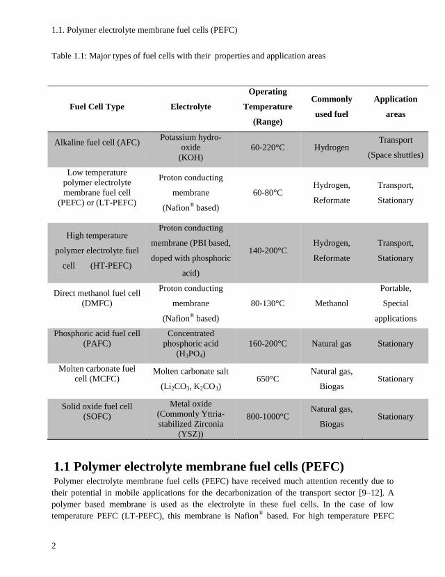
1.1. Polymer electrolyte membrane fuel cells (PEFC)
2
Table 1.1: Major types of fuel cells with their properties and application areas
1.1 Polymer electrolyte membrane fuel cells (PEFC) Polymer electrolyte membrane fuel cells (PEFC) have received much attention recently due to
their potential in mobile applications for the decarbonization of the transport sector [9–12]. A
polymer based membrane is used as the electrolyte in these fuel cells. In the case of low
temperature PEFC (LT-PEFC), this membrane is Nafion®
based. For high temperature PEFC
Fuel Cell Type Electrolyte
Operating
Temperature
(Range)
Commonly
used fuel
Application
areas
Alkaline fuel cell (AFC)
Potassium hydro-
oxide
(KOH)
60-220°C Hydrogen Transport
(Space shuttles)
Low temperature
polymer electrolyte
membrane fuel cell
(PEFC) or (LT-PEFC)
Proton conducting
membrane
(Nafion®
based)
60-80°C Hydrogen,
Reformate
Transport,
Stationary
High temperature
polymer electrolyte fuel
cell (HT-PEFC)
Proton conducting
membrane (PBI based,
doped with phosphoric
acid)
140-200°C Hydrogen,
Reformate
Transport,
Stationary
Direct methanol fuel cell
(DMFC)
Proton conducting
membrane
(Nafion®
based)
80-130°C Methanol
Portable,
Special
applications
Phosphoric acid fuel cell
(PAFC)
Concentrated
phosphoric acid
(H3PO4)
160-200°C Natural gas Stationary
Molten carbonate fuel
cell (MCFC)
Molten carbonate salt
(Li2CO3, K2CO3) 650°C
Natural gas,
Biogas Stationary
Solid oxide fuel cell
(SOFC)
Metal oxide
(Commonly Yttria-
stabilized Zirconia
(YSZ))
800-1000°C Natural gas,
Biogas Stationary
1. Introduction and Literature Review
3
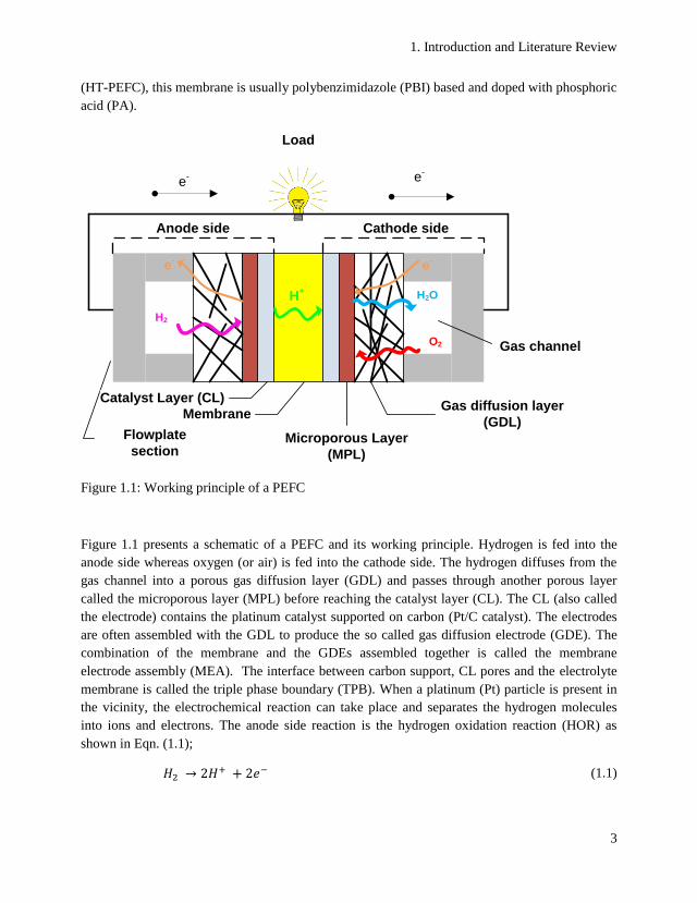
(HT-PEFC), this membrane is usually polybenzimidazole (PBI) based and doped with phosphoric
acid (PA).
Membrane
Anode side Cathode side
e-
e-
H2
H2O
O2
H+
Gas channel
Gas diffusion layer
(GDL)Flowplate
section
e- e
-
Load
Catalyst Layer (CL)
Microporous Layer
(MPL)
Figure 1.1: Working principle of a PEFC
Figure 1.1 presents a schematic of a PEFC and its working principle. Hydrogen is fed into the
anode side whereas oxygen (or air) is fed into the cathode side. The hydrogen diffuses from the
gas channel into a porous gas diffusion layer (GDL) and passes through another porous layer
called the microporous layer (MPL) before reaching the catalyst layer (CL). The CL (also called
the electrode) contains the platinum catalyst supported on carbon (Pt/C catalyst). The electrodes
are often assembled with the GDL to produce the so called gas diffusion electrode (GDE). The
combination of the membrane and the GDEs assembled together is called the membrane
electrode assembly (MEA). The interface between carbon support, CL pores and the electrolyte
membrane is called the triple phase boundary (TPB). When a platinum (Pt) particle is present in
the vicinity, the electrochemical reaction can take place and separates the hydrogen molecules
into ions and electrons. The anode side reaction is the hydrogen oxidation reaction (HOR) as
shown in Eqn. (1.1);
𝐻2 → 2𝐻+ + 2𝑒− (1.1)
1.1. Polymer electrolyte membrane fuel cells (PEFC)
4
The oxygen on the cathode side also reaches the TPBs after passing through the GDE on the
cathode side. The hydrogen ions produced on the anode side pass through the proton conducting
membrane to the cathode side, whereas the electrons pass through an outer route through a load
to the cathode side, thereby producing an electric current which can be utilized. The hydrogen
ions, electrons and oxygen combine on the cathode side for the oxygen reduction reaction (ORR)
and formation of water as follows;
1
2𝑂2 + 2𝐻+ + 2𝑒− → 𝐻2𝑂 (1.2)
The overall reaction of the PEFC is also called a Redox reaction and is given by Eqn. (1.3)
below;
𝐻2 + 1
2𝑂2 → 𝐻2𝑂 + 𝐻𝑒𝑎𝑡 (1.3)
Thermodynamically, the heat or enthalpy change (ΔH) of the chemical reaction in the PEFC can
be given as;
∆𝐻 = ∆𝐺 + 𝑇∆𝑆 (1.4)
Where,
ΔG = change in Gibbs free energy of the reaction (kJ mol-1
)
T = reaction temperature (K)
ΔS = change in entropy of the reaction (kJ mol-1
K-1
)
The Gibbs free energy represents the maximum energy available for utilization as electrical
energy in the fuel cell and therefore, the maximum theoretical efficiency (ηmax) of the fuel cell
can be calculated as;
𝜂𝑚𝑎𝑥 = ∆𝐺
∆𝐻 (1.5)
The values of ∆𝐺 and ∆𝐻 for standard temperature and pressure (STP) conditions (1atm and
298K) for production of water in liquid or vapor state are different. The value of ∆𝐻 related to
liquid water production is called the higher heating value (HHV) of hydrogen (286.02kJ mol-1
)
and the value related to water vapor production is called the lower heating value (LHV) of
hydrogen (241.98kJ mol-1
) [13]. The maximum theoretical efficiency of the PEFC when
calculated with the HHV of hydrogen is about 83% and 94.5% when calculated using the LHV of
hydrogen.
The theoretical fuel cell potential is given by;
1. Introduction and Literature Review
5
𝐸0 = −∆𝐺
𝑛 ∙ 𝐹 (1.6)
Where,
E0 = Theoretical fuel cell potential (Volts)
n = number of electrons per molecule of H2 = 2
F (Faraday’s constant) = 96485C mol-1
So the theoretical fuel cell potential for hydrogen/oxygen fuel cell comes out to be 1.23V at STP.
However, real fuel cell operation is seldom under STP conditions and the dependence of the
Gibbs free energy on temperature and pressure is stipulated on the cell potential through the
following form of the Nernst equation;
𝐸 = 𝐸0 + 𝑅𝑇
𝑛𝐹∙ 𝑙𝑛 (
𝑃𝐻2𝑃𝑂2
0.5
𝑃𝐻2𝑂) (1.7)
Where,
E = Nernst fuel cell potential (Volts)
R (Universal gas constant) = 8.314J mol-1
K-1
T = Operating temperature of the fuel cell (K)
PH2, PO2, PH2O = normalized partial pressures (𝑝𝑖
𝑝0) of hydrogen, oxygen and water vapor, where
p0 is atmospheric pressure
Eqn. (1.7) is valid for reactants and product water in gaseous state. For water produced in liquid
state, PH2O =1. The actual fuel cell potential is different from the Nernst potential due to
characteristic losses encountered during fuel cell operation. These losses can be divided into three
categories and the regions dominated by them can be readily identified in a polarization curve,
which is a plot of the fuel cell voltage against the current density.
1.1. Polymer electrolyte membrane fuel cells (PEFC)
6
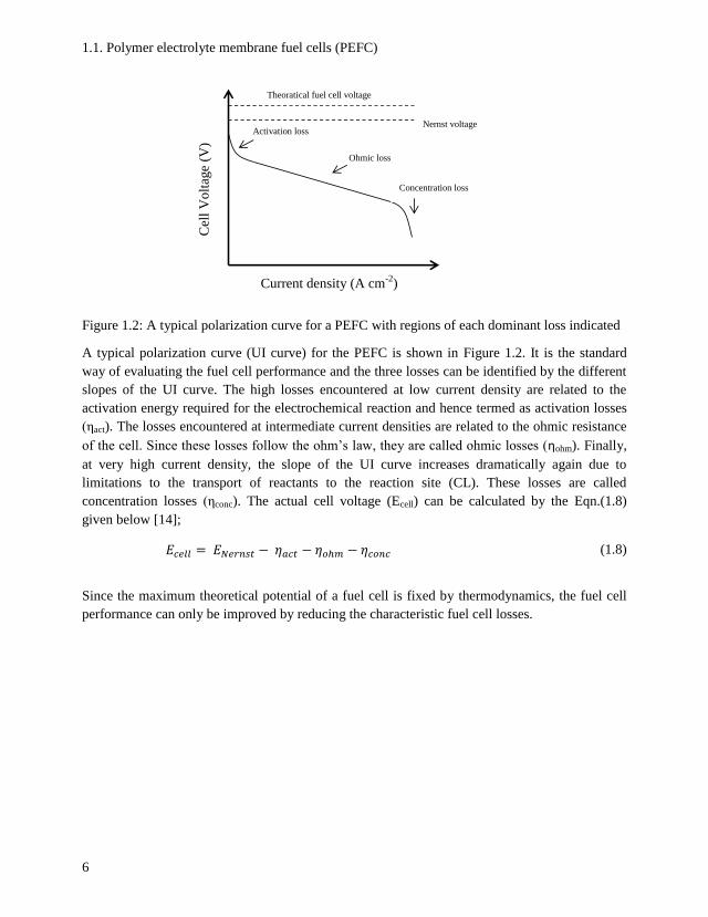
Figure 1.2: A typical polarization curve for a PEFC with regions of each dominant loss indicated
A typical polarization curve (UI curve) for the PEFC is shown in Figure 1.2. It is the standard
way of evaluating the fuel cell performance and the three losses can be identified by the different
slopes of the UI curve. The high losses encountered at low current density are related to the
activation energy required for the electrochemical reaction and hence termed as activation losses
(ηact). The losses encountered at intermediate current densities are related to the ohmic resistance
of the cell. Since these losses follow the ohm’s law, they are called ohmic losses (ηohm). Finally,
at very high current density, the slope of the UI curve increases dramatically again due to
limitations to the transport of reactants to the reaction site (CL). These losses are called
concentration losses (ηconc). The actual cell voltage (Ecell) can be calculated by the Eqn.(1.8)
given below [14];
𝐸𝑐𝑒𝑙𝑙 = 𝐸𝑁𝑒𝑟𝑛𝑠𝑡 − 𝜂𝑎𝑐𝑡 − 𝜂𝑜ℎ𝑚 − 𝜂𝑐𝑜𝑛𝑐 (1.8)
Since the maximum theoretical potential of a fuel cell is fixed by thermodynamics, the fuel cell
performance can only be improved by reducing the characteristic fuel cell losses.
Nernst voltage Activation loss
Ohmic loss
Concentration loss
Current density (A cm-2
)
Cel
l V
olt
age
(V)
Theoratical fuel cell voltage
1. Introduction and Literature Review
7
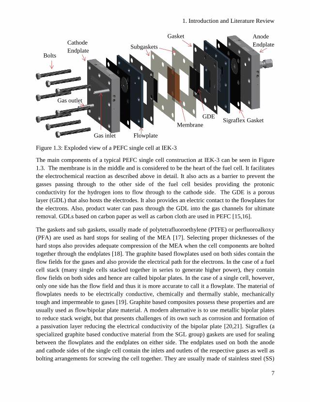
Figure 1.3: Exploded view of a PEFC single cell at IEK-3
The main components of a typical PEFC single cell construction at IEK-3 can be seen in Figure
1.3. The membrane is in the middle and is considered to be the heart of the fuel cell. It facilitates
the electrochemical reaction as described above in detail. It also acts as a barrier to prevent the
gasses passing through to the other side of the fuel cell besides providing the protonic
conductivity for the hydrogen ions to flow through to the cathode side. The GDE is a porous
layer (GDL) that also hosts the electrodes. It also provides an electric contact to the flowplates for
the electrons. Also, product water can pass through the GDL into the gas channels for ultimate
removal. GDLs based on carbon paper as well as carbon cloth are used in PEFC [15,16].
The gaskets and sub gaskets, usually made of polytetrafluoroethylene (PTFE) or perfluoroalkoxy
(PFA) are used as hard stops for sealing of the MEA [17]. Selecting proper thicknesses of the
hard stops also provides adequate compression of the MEA when the cell components are bolted
together through the endplates [18]. The graphite based flowplates used on both sides contain the
flow fields for the gases and also provide the electrical path for the electrons. In the case of a fuel
cell stack (many single cells stacked together in series to generate higher power), they contain
flow fields on both sides and hence are called bipolar plates. In the case of a single cell, however,
only one side has the flow field and thus it is more accurate to call it a flowplate. The material of
flowplates needs to be electrically conductive, chemically and thermally stable, mechanically
tough and impermeable to gases [19]. Graphite based composites possess these properties and are
usually used as flow/bipolar plate material. A modern alternative is to use metallic bipolar plates
to reduce stack weight, but that presents challenges of its own such as corrosion and formation of
a passivation layer reducing the electrical conductivity of the bipolar plate [20,21]. Sigraflex (a
specialized graphite based conductive material from the SGL group) gaskets are used for sealing
between the flowplates and the endplates on either side. The endplates used on both the anode
and cathode sides of the single cell contain the inlets and outlets of the respective gases as well as
bolting arrangements for screwing the cell together. They are usually made of stainless steel (SS)
Membrane
Subgaskets
GDE
Gasket
Sigraflex Gasket
Flowplate
Anode
Endplate Cathode
Endplate Bolts
Gas inlet
Gas outlet
1.1. Polymer electrolyte membrane fuel cells (PEFC)
8
and hold the fuel cell components together and provide mechanical stability to them. They are
also used to accommodate heating elements for heating the cell as well as thermocouples for
measuring the cell temperature during operation.
1.1.1 Comparison of LT-PEFC and HT-PEFC The PEFC can be further classified into LT-PEFC and HT-PEFC with the main differences being
the electrolyte membrane (Nafion®
based for LT-PEFC while PBI based doped with PA for HT-
PEFC) and the operating temperatures at atmospheric pressure as listed in Table 1.1. The proton
conductivity of the Nafion®
based membrane is highly dependent on the liquid water content of
the membrane [22]. The fuel cell must be operated below the boiling point of water within a
narrow window of operating temperature (about 60-80oC at 1 atm) due to a dramatic increase in
voltage loss above 90oC [23]. These limitations necessitate LT-PEFC operation below this
temperature and also the inlet gases must be humidified and complex water and heat management
systems must be employed for constant water and heat removal for the proper functioning of the
fuel cell [24–27]. The sluggish reaction kinetics of the ORR is also considered to be a major
challenge for better PEFC operation and commercialization [28–31].
High temperature operation presents many advantages such as improved reaction kinetics, much
higher tolerance to fuel impurities like carbon monoxide (CO), little need for humidification of
inlet gases and much simpler heat and water management [32–35]. The HT-PEFC is designed
for high temperature operation to harness some of these advantages by employing a PBI based
membrane doped with phosphoric acid (PA) as the electrolyte. The protonic conductivity of this
membrane does not depend on liquid water and is mainly provided by the PA, which can
maintain good protonic conductivity upto 200oC [36]. The HT-PEFC can therefore be operated at
temperatures from 140oC upto 200
oC at atmospheric pressure and with dry gases [37]. Also, CO
tolerance in the fuel stream of the HT-PEFC is 1 to 3% [38–44], which is much higher than
the LT-PEFC, whose performance can be significantly affected by as little as 5-10 ppm of CO in
the fuel stream [45]. This allows the use of a hydrogen rich gas (reformate) containing CO within
the range tolerable by HT-PEFC, produced by reforming onboard fuels in heavy transport
applications, as the fuel in HT-PEFC stacks for auxiliary power generation [46].
There are not many direct comparisons published in the literature between the performance of
LT-PEFC and HT-PEFC at the single cell level. However, Zhu et al. [47] compared the
performance of an LT-PEFC and HT-PEFC stack by electrochemical impedance spectroscopy
(EIS) and determined that the ORR reaction kinetics of the HT-PEFC stack was much better.
Authayanun et al. [48] compared HT-PEFC and LT-PEFC systems integrated with a glycerol
steam reformer. They determined that the LT-PEFC system performed better under pure
hydrogen operation and atmospheric pressure, but the HT-PEFC system performed better under
high current density operation as well as pressurized and reformate operation. The HT-PEFC
system with a water gas shift reactor also showed the highest system efficiency (60%) for the
systems tested. Further comparative studies and investigation is required for a broader
understanding of the effect of temperature on the rate of ORR at the single cell, stack and system
1. Introduction and Literature Review
9
level. Also, a common testing and comparison protocol among various research groups and the
industry would help standardize such investigations.
1.1.2 Challenges faced by the HT-PEFC and current research A lot of research has been conducted recently in the field of HT-PEFCs due to their potential
advantages as discussed in the previous section. The higher operating temperature also causes
some serious challenges for the HT-PEFC. This includes much longer start-up times in
comparison with LT-PEFC [49,50], which is critical for transport applications. The degradation
rates of cell components are also much higher [32,35], with severe degradation expected for
operation above 180oC [33] . Loss of PA due to PA leaching [51] , uptake of the PA by the
bipolar plates [18], dehydration and unfavorable redistribution of PA [52–54] in the MEA is also
a main cause for lower performance and MEA degradation. Pt particle size growth due to
agglomeration at elevated temperatures has also been reported as a major cause of performance
degradation [55,56]. Pt dissolution also causes loss of electrochemical surface area (ECSA) at
high temperature operation [57,58]. Severe corrosion of the carbon support of the Pt catalyst
takes place at the cathode at high potential and high oxygen partial pressure [59,60]. This can
cause a significant loss in ECSA and thus cause significant irreversible losses in the fuel cell
performance [61,62]. Carbon corrosion can also effect the GDL material and cause loss of
hydrophobicity [63] resulting in pore blockage and possible flooding of the GDL at higher
current densities, thus reducing the operational window of the fuel cell. Thinning of the PBI
membrane [64] and creep failure has also been reported in the literature as a major cause of
membrane degradation [55,65–67]. The adsorption of phosphate anions onto the Pt surface is also
an area of serious concern for HT-PEFC operation [68,69].
Most of the current research in the field of HT-PEFC is focused on resolving the issues faced by
the HT-PEFC as described in the previous paragraph. At the component level, there has been a
lot of research on membranes with higher protonic conductivity and more thermal, chemical and
mechanical stability for increased longevity. Ozdemir et al. [70] achieved a protonic conductivity
of 0.2S cm-1
and improved thermal stability by dispersion of 5 wt. % ZrP nanoparticles in the PBI
polymer before doping with phosphoric acid to obtain a high phosphoric acid doping level
(PADL). The GDE is also a vital component of the MEA with several important functions as
described previously. Mazur et al. [71] optimized the preparation procedure and chemical
composition of the GDE for HT-PEFC and found spraying and brushing to be the most effective
methods for CL deposition. They also tested PTFE and PBI as binder materials and found similar
performance of the GDEs prepared by the spraying method with each binder. Lowering the Pt
loading of the CL of the HT-PEFC is of utmost importance from a cost viewpoint. Martin et al.
[72] achieved a stable performance of a HT-PEFC for over 1700 hours with a Pt loading of
0.1mg cm-2
by using no binder material to prepare the CL. Zamora et al. [73] demonstrated
improved electrochemical stability of the MPL by using carbon nanostructures (CNS) based
MPLs and comparing it to carbon black (CB) based MPLs.
1.1. Polymer electrolyte membrane fuel cells (PEFC)
10
Studying the effects of various operating conditions on fuel cell performance is vital for
determining the best operational window. Yan et al. [74] compared the steady state and dynamic
performance of a LT-PEFC single cell under widely varying operating conditions. They tested
the cell performance with different feed gas humidity and stoichiometry, operating temperature,
operating pressure and fuel cell size. They used polarization curves and EIS to analyze and
compare the cell performance at different operating conditions and determined the optimum level
for each operating condition. Zhang et al. [75] compared the steady state and dynamic behavior
of a HT-PEFC by comparing cell performance in flow-through mode and dead end mode. Rastedt
et al. [76] investigated the effect of contact pressure cycling between 0.2 and 1.5MPa on single
cell performance with a non-woven GDL. They determined a correlation between the loss of
internal resistance and hydrogen crossover current and the emergence of small cracks and fiber
intrusions in the GDL. Andreasen et al. [77] analyzed the performance of a single cell with
varying CO, CO2 and H2 content in the anode gas by utilizing EIS. They measured impedance at
different operating temperatures and currents in addition to the anode gas composition and found
undesirable transient effects for measurements conducted at low temperatures and high CO
content in the anode gas. Taccani et al. [78] investigated the effects of different flow field
geometries on single cell performance and found that using a serpentine flow field results in
better performance than a parallel flow field but also causes higher pressure drop. Finally,
Korsgaard et al [79] developed a semi empirical model for fuel cell voltage versus current
density, cathode stoichiometry and operating temperature by using linear regression and found
excellent agreement with the experimental values.
Determination of the electrochemical parameters representing the electrode performance is a very
useful way of understanding the causes of lower fuel cell performance. Mitigation strategies can
then be developed for the isolated causes. EIS has been used successfully by many researchers
around the world not only for this purpose, but also to identify and isolate different
electrochemical processes within the cell, although the models used for fitting EIS data and the
interpretation of the results differ considerably. Numerical, analytical and equivalent circuit
models (ECM) have been used in the literature for fitting EIS data. Springer et al. [80] applied
EIS to differentiate between the three different types of PEFC losses in the low and high
frequency loops present in typical impedance spectra. Makharia et al. [81] applied the
transmission line model to extract the ohmic resistance, catalytic layer electrolyte resistance and
the double layer capacitance by fitting EIS data of a PEFC. Yi et al. [82] presented a numerical
model based analysis of EIS data of PEFC to determine the charge transfer resistance, protonic
resistance and the double layer capacitance along the thickness of the CL. Kulikovsky [83]
presented an exact solution based analytical model for PEFC cathode impedance at low current
densities and high cathode stoichiometry. EIS continues to be an intense area of research due to
its powerful in situ characterization potential for PEFC, but interpretation of EIS data with simple
and reliable fitting models for extraction of physically relevant fuel cell electrochemical
parameters remains disputed.
1. Introduction and Literature Review
11
Degradation of HT-PEFC is a very important issue since the higher operating temperature causes
faster degradation of cell components. Modestov et al. [55] determined Pt particle growth as the
main cause of degradation in a 780 hour life test of a HT-PEFC with more than double increase
in the average Pt particle size. Galbiati et al. [84] determined that increased gas crossover and
short circuit currents were the main causes of performance loss for the HT-PEFC in a 600 hour
parametric test. Sondergaard et al. [85] found a correlation between the operating temperature
and the accumulated gas-flow volume through the HT-PEFC and loss of PA by evaporation.
They determined the loss of PA as the major degradation mechanism. Ossiander et al. [86]
examined the effect of molecular weight and different reinforcement strategies for PBI based
membranes and achieved significant reduction in degradation by enhancing the interactions
between PBI polymer chains by cross-linking. Tang et al. [87] used a single and dual cell
configuration to measure cathode potentials as high as twice the open circuit voltage in PEFC
during startup and shutdown due to the air/fuel boundary developed at the anode. They
determined the carbon corrosion at the cathode as the main degradation mechanism at high
potentials. Eberhardt et al. [88] found the loss of PA to be only a function of gas flowrates and
operating temperature. They suggested a PA management strategy to be employed for operating
temperatures higher than 160oC at high current densities in HT-PEFC to achieve the 50,000 hour
lifetime goal of the US department of energy for HT-PEFC. Accelerated degradation testing
helps determine the main causes of degradation in a relatively small amount of time so that
relevant mitigation strategies can be formulated to achieve lifetime goals for HT-PEFC set by the
department of energy of United States. Reimer et al. [61] used load cycling to investigate four
different HT-PEFC single cells. They used a simple polarization curve model to explore different
possible degradation mechanisms. They concluded that loss of PA due to overall heat flux was a
more likely interpretation under the operating conditions used than corrosion of the carbon based
catalyst support due to high potential. De Beer et al. [63] used an accelerated acid leaching
procedure to investigate degradation in HT-PEFC. Zhou et al. [89] used hydrogen starvation as
the stressor to investigate HT-PEFC degradation. Park et al. [90] tested the mechanical stability
of PBI based membranes under thermal cycling conditions and found that PBI composite
membranes with pretreated PTFE had lower degradation rates than membranes with untreated
PTFE. High temperature operation, start/stop cycling and potential cycling have also been
applied as stressors to HT-PEFC for accelerated degradation testing.
1.2 Motivation and experimental goals As discussed in the previous section, there are many areas of improvement for HT-PEFC
operation. This thesis is mainly concerned with addressing some of the challenges faced by
HT-PEFC as described above. The focus is at the MEA level and the experiments concentrate on
identifying the effects of important operational and material parameters on the MEA performance
in single cell operation. The underlying physical phenomena are identified and ideas for
improvement are developed and tested. The overall goal of this study is to suggest ways to
improve the long term single cell performance of the HT-PEFC by;

1.2. Motivation and experimental goals
12
Identifying the effects of important operational parameters on the performance of the fuel
cell and selecting the most suitable operating conditions for long term operation.
Investigating the material parameters of the MEA and their interactions to compare the
effect of different combinations of these parameters and suggest the best combinations.
Minimizing the cell resistance by studying the effects of different operating conditions on
characteristic electrochemical parameters related to the cathode catalyst layer (CCL)
using EIS.
Examining the effect of different stressors on fuel cell performance degradation and
identifying the underlying degradation mechanisms for the development of mitigation
strategies.
These four goals lead to the experimental studies presented in chapters 4, 5, 6 and 7. Chapter 4
addresses the issue of determination of the best operating conditions for fuel cell operation as
well as development of statistical models to predict the cell performance with a small amount of
experimental data available by utilizing the design of experiments (DoE). Chapter 5 is devoted to
investigation of the effects of the most important material parameters on MEA performance and
evaluation of their interactions and effects on cell impedance by the DoE and EIS methods.
Chapter 6 covers the effects of gas composition on cell impedance and compares the different
electrochemical parameters determined by the ECM and analytical models for analyzing EIS
data. Finally, in chapter 7, a short accelerated degradation study is conducted to determine the
effects of various stressors on cell performance and postulate some of the related degradation
mechanisms and mitigation strategies.
13
2 Experimental Methods
This chapter presents the two most extensively used experimental methods in this thesis, the
design of experiments (DoE) and electrochemical impedance spectroscopy (EIS) in detail.
2.1 Design of experiments (DoE)
2.1.1 One factor at a time (OFAT) method and DoE comparison Fuel cell technology is a relatively complex field with electrochemistry, heat transfer, fluid
mechanics and structural mechanics playing an important part among others in the overall cell
performance. Also, as the search for cheaper and more efficient materials goes on, there are a
large number of material and operating parameters which can affect the fuel cell performance.
The traditional method used for investigating the effect of different variables on an output
variable of interest has been the one factor at a time (OFAT) method. The procedure is to hold all
variables constant except one, and then study the effect of varying this variable on the output
variable. This method works well for a small number of variables. However, an increase in the
number of variables to be analyzed requires a greater experimental effort, which is sometimes
unrealistic. Another drawback of the OFAT method is the inability to determine interactions
among the studied variables (different effect of varying a variable on the output variable, when
another variable has a different value), which may be very important in some cases. Disregarding
interactions may lead to incorrect interpretation of the obtained results. The DoE is a statistical
approach to planning and analyzing scientific experiments, with many advantages. As most of the
experimental characterization in fuel cell materials and operation usually involves a large number
of variables, it is suggested as an alternative approach to the OFAT method. DoE has been
around for quite a while now, especially in industrial quality control, where it is routinely a part
of product and process improvement campaigns with a large number of variables. The DoE has
the twofold advantage of not only reducing the experimental effort required for a large number of
variables, but also yielding more reliable results in the cases where interactions are significant.
The DoE method has enormous potential for application in the field of fuel cells and electrolyzers
due to its versatility and suitability to the wide range of variables usually involved in typical
characterization campaigns.
In DoE terminology, the independent variables, whose effect on the output is desired to be
analyzed, are called factors. The dependent variable or the output, whose change with respect to
the factors is to be analyzed, is called the response. Multiple responses can also be analyzed
simultaneously. The effect of each factor on the response in isolation is called its main effect. The
effect on two or more factors combined is called a factor interaction. Although, higher order
factor interactions (involving 3 or more factors) exist for a DoE with k factors, usually the most
important ones are the two factor interactions. Interactions involving more than two factors are
2.1. Design of experiments (DoE)
14
usually assigned to random noise and used as degrees of freedom for calculating the experimental
error [91–93].
The so called 2k design of the DoE refers to the case with k factors, each with 2 levels. These
levels are usually carefully selected minimum and maximum values of interest of the factor, but
they can also be qualitative attributes. The DoE can be either a full factorial or a fractional
factorial depending on the number of experiments conducted. A full factorial design has the
maximum number of experiments and also the maximum detail possible in the results, whereas a
fractional factorial can be conducted with lesser number of experiments but the level of detail and
accuracy is also reduced.
It is easy to verify that as the number of factors increases, the experimental effort required for the
OFAT method increases many-fold. This renders planning and executing an effective
experimental plan very tedious if not impossible when a large number of factors are involved.
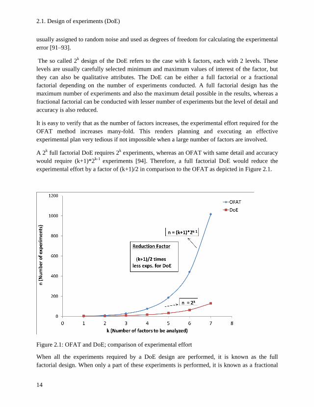
A 2k full factorial DoE requires 2
k experiments, whereas an OFAT with same detail and accuracy
would require (k+1)*2k-1
experiments [94]. Therefore, a full factorial DoE would reduce the
experimental effort by a factor of (k+1)/2 in comparison to the OFAT as depicted in Figure 2.1.
Figure 2.1: OFAT and DoE; comparison of experimental effort
When all the experiments required by a DoE design are performed, it is known as the full
factorial design. When only a part of these experiments is performed, it is known as a fractional

2. Experimental Methods
15
factorial design. A fractional factorial design is preferred in the case of a large number of factors
or expected linearity of the process under investigation [95].
It is evident from the above discussion that DoE should be the preferred method for dealing with
a large number of variables. Nevertheless, it is still far from being the universally accepted
methodology and there remains plenty of untapped potential for application of DoE in all areas of
fuel cell research, mainly due to lack of knowledge and resistance to change, given its clear
superiority over OFAT for experimental campaigns with a large number of factors. This is so,
because, the DoE not only optimizes the experimental process itself by reducing the required
number of experiments to a manageable minimum, but also improves the reliability and
repeatability of the results by including the effects of factor interactions in the results alongside
the main effects of the investigated factors.
2.1.2 DoE approaches and methodology There are three main approaches to applying the DoE method to experimentation. These are the
classical approach, the Taguchi approach and the Shainin system TM
. The classical approach was
first developed and used by R.A. Fischer in 1920 [96] to an agricultural problem to produce the
best crop of potatoes by analyzing many factors affecting the crop. The Taguchi approach was
first published in Japan and gained popularity in the west after the 1980s. The Shainin system TM
is a legally protected system with little literature available. The Taguchi and Shainin approaches
may be considered quality improvement strategies rather than just experimental designs [97] and
their use in the industry for various purposes, especially quality control is increasing. The
classical approach is especially suitable, valid and robust in the case of cheap experimentation or
a small (less than five) number of factors or both [98]. Through the contributions of many
scientists and authors, this remains to be true till this day with classical textbooks from Hunter et
al. [91] and Montgomery [92] available for reference. All the three approaches to applying the
DoE are superior to the OFAT methodology [98]. The response surface methodology (RSM) as
developed by Box & Wilson [99], enhanced the classical approach by providing the ability to
obtain results quickly and plan the experiments sequentially to improve new experimental
designs on the basis of the results from the previous experiments [92]. The classical approach is
followed in this thesis since the number of factors is small and experimental costs are also not
prohibiting. Also, most of the literature and software available about DoE presume the classical
approach.
2.1. Design of experiments (DoE)
16
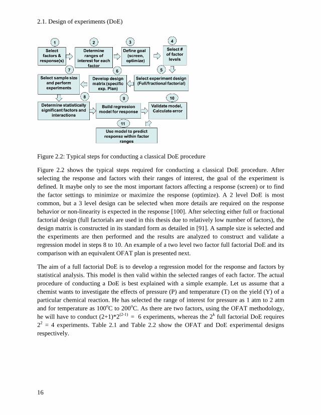
Figure 2.2: Typical steps for conducting a classical DoE procedure
Figure 2.2 shows the typical steps required for conducting a classical DoE procedure. After
selecting the response and factors with their ranges of interest, the goal of the experiment is
defined. It maybe only to see the most important factors affecting a response (screen) or to find
the factor settings to minimize or maximize the response (optimize). A 2 level DoE is most
common, but a 3 level design can be selected when more details are required on the response
behavior or non-linearity is expected in the response [100]. After selecting either full or fractional
factorial design (full factorials are used in this thesis due to relatively low number of factors), the
design matrix is constructed in its standard form as detailed in [91]. A sample size is selected and
the experiments are then performed and the results are analyzed to construct and validate a
regression model in steps 8 to 10. An example of a two level two factor full factorial DoE and its
comparison with an equivalent OFAT plan is presented next.
The aim of a full factorial DoE is to develop a regression model for the response and factors by
statistical analysis. This model is then valid within the selected ranges of each factor. The actual
procedure of conducting a DoE is best explained with a simple example. Let us assume that a
chemist wants to investigate the effects of pressure (P) and temperature (T) on the yield (Y) of a
particular chemical reaction. He has selected the range of interest for pressure as 1 atm to 2 atm
and for temperature as 100oC to 200
oC. As there are two factors, using the OFAT methodology,
he will have to conduct (2+1)*2(2-1)
= 6 experiments, whereas the 2k full factorial DoE requires
22 = 4 experiments. Table 2.1 and Table 2.2 show the OFAT and DoE experimental designs
respectively.
2. Experimental Methods
17
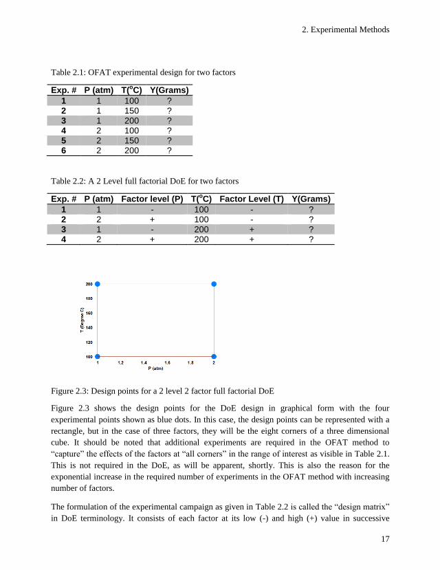
Table 2.1: OFAT experimental design for two factors
Exp. # P (atm) T(oC) Y(Grams)
1 1 100 ? 2 1 150 ? 3 1 200 ? 4 2 100 ? 5 2 150 ? 6 2 200 ?
Table 2.2: A 2 Level full factorial DoE for two factors
Exp. # P (atm) Factor level (P) T(oC) Factor Level (T) Y(Grams)
1 1 - 100 - ? 2 2 + 100 - ? 3 1 - 200 + ? 4 2 + 200 + ?
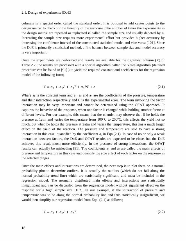
Figure 2.3: Design points for a 2 level 2 factor full factorial DoE
Figure 2.3 shows the design points for the DoE design in graphical form with the four
experimental points shown as blue dots. In this case, the design points can be represented with a
rectangle, but in the case of three factors, they will be the eight corners of a three dimensional
cube. It should be noted that additional experiments are required in the OFAT method to
“capture” the effects of the factors at “all corners” in the range of interest as visible in Table 2.1.
This is not required in the DoE, as will be apparent, shortly. This is also the reason for the
exponential increase in the required number of experiments in the OFAT method with increasing
number of factors.
The formulation of the experimental campaign as given in Table 2.2 is called the “design matrix”
in DoE terminology. It consists of each factor at its low (-) and high (+) value in successive
2.1. Design of experiments (DoE)
18
columns in a special order called the standard order. It is optional to add center points to the
design matrix to check for the linearity of the response. The number of times the experiments in
the design matrix are repeated or replicated is called the sample size and usually denoted by n.
Increasing the sample size requires more experimental effort but provides higher accuracy by
increasing the confidence interval of the constructed statistical model and vice versa [101]. Since
the DoE is primarily a statistical method, a fine balance between sample size and model accuracy
is very important.
Once the experiments are performed and results are available for the rightmost column (Y) of
Table 2.2, the results are processed with a special algorithm called the Yates algorithm (detailed
procedure can be found in [91] ) to yield the required constant and coefficients for the regression
model of the following form;
𝑌 = 𝑎0 + 𝑎1𝑃 + 𝑎2𝑇 + 𝑎3𝑃𝑇 + 𝜀 (2.1)
Where a0 is the constant term and a1, a2 and a3 are the coefficients of the pressure, temperature
and their interaction respectively and Ɛ is the experimental error. The term involving the factor
interaction may be very important and cannot be determined using the OFAT approach. It
captures the behavior of the response, when one factor is changed while holding another factor at
different levels. For our example, this means that the chemist may observe that if he holds the
pressure at 1atm and varies the temperature from 100oC to 200
oC, this affects the yield not so
much, but when he holds the pressure at 2atm and varies the temperature, this has a much larger
effect on the yield of the reaction. The pressure and temperature are said to have a strong
interaction in this case, quantified by the coefficient a3 in Eqn.(2.1). In case of no or only a weak
interaction between factors, the DoE and OFAT results are expected to be close, but the DoE
achieves this result much more efficiently. In the presence of strong interactions, the OFAT
results can actually be misleading [91]. The coefficients a1 and a2 are called the main effects of
pressure and temperature in this case and quantify the sole effect of each factor on the response in
the selected ranges.
Once the main effects and interactions are determined, the next step is to plot them on a normal
probability plot to determine outliers. It is actually the outliers (which do not fall along the
normal probability trend line) which are statistically significant, and must be included in the
regression model. The normally distributed main effects and interactions are statistically
insignificant and can be discarded from the regression model without significant effect on the
response for a high sample size [102]. In our example, if the interaction of pressure and
temperature was to be along the normal probability line and thus statistically insignificant, we
would then simplify our regression model from Eqn. (2.1) as follows;
𝑌 = 𝑎0 + 𝑎1𝑃 + 𝑎2𝑇 (2.2)
2. Experimental Methods
19
Eqn. (2.2) is the required regression model for the evaluation of the yield within the selected
ranges of temperature and pressure. However, if the interaction is not normally distributed and
thus statistically significant, then the regression model would contain the additional term of the
interaction with its coefficient a3 as given below in Eqn. (2.3);
𝑌 = 𝑎0 + 𝑎1𝑃 + 𝑎2𝑇 + 𝑎3𝑃𝑇 + 𝜀 (2.3)
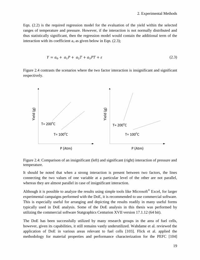
Figure 2.4 contrasts the scenarios where the two factor interaction is insignificant and significant
respectively.
Yiel
d (
g)
P (Atm)
T= 200oC
T= 100oC
Yiel
d (
g)
P (Atm)
T= 200oC
T= 100oC
Figure 2.4: Comparison of an insignificant (left) and significant (right) interaction of pressure and
temperature.
It should be noted that when a strong interaction is present between two factors, the lines
connecting the two values of one variable at a particular level of the other are not parallel,
whereas they are almost parallel in case of insignificant interaction.
Although it is possible to analyze the results using simple tools like Microsoft®
Excel, for larger
experimental campaigns performed with the DoE, it is recommended to use commercial software.
This is especially useful for arranging and depicting the results readily in many useful forms
typically used in DoE analysis. Some of the DoE analysis in this thesis was performed by
utilizing the commercial software Statgraphics Centurion XVII version 17.1.12 (64 bit).
The DoE has been successfully utilized by many research groups in the area of fuel cells,
however, given its capabilities, it still remains vastly underutilized. Wahdame et al. reviewed the
application of DoE in various areas relevant to fuel cells [103]. Flick et al. applied the
methodology for material properties and performance characterization for the PEFC [104]
2.2. Electrochemical impedance spectroscopy (EIS)
20
whereas Kahveci et al. applied response surface methodology to water and heat management
investigations in PEFC [105]. Lohoff et al. applied the DoE methodology for the characterization
of a DMFC stack [106] and finally, Barari et al. applied DoE to improve the temperature
measurement accuracy in a SOFC [107].The list is long, but this should suffice as evidence of the
growing popularity of application of DoE in fuel cell research worldwide.
2.2 Electrochemical impedance spectroscopy (EIS) Electrochemical impedance spectroscopy (EIS) is a powerful in-situ technique for the
characterization of interfacial processes involving redox reactions at electrodes. EIS is a special
electrochemical method as it presents the signal as a function of frequency at a constant voltage
(or current) in contrast to classical electrochemical methods, which present current, voltage or
charges as a function of time. This provides a potentially large amount of information about the
behavior of the process under study at different frequencies, but special techniques and
knowledge is required for the correct interpretation of this data and there exists significant
difference of opinion in this regard. This is one of the reasons that EIS data is not always
analyzed or interpreted in a similar fashion in the literature.
In the case of fuel cells it can be used to isolate and quantify the three main sources of voltage
loss in fuel cells; the activation loss Ract, the ohmic loss RΩ and the mass transport loss Rm, as
well as the charge storing capacity of the electrode/electrolyte interface (termed as the double
layer capacitance (Cdl) in most fuel cell literature). The physiochemical processes causing the
losses have unique characteristic time constants due to the nature of the process and thus occur at
different AC frequencies. Therefore, they can be easily identified in the impedance data and the
information gained can then be used to minimize the losses and improve fuel cell performance.
2.2.1 EIS basics Electrochemical systems are inherently non-linear systems. However, if a small enough voltage
or current perturbation is applied, the response of the system is almost linear. This is called
pseudo linearity. EIS measurements of electrochemical systems utilize the pseudo linearity of
their response for very small AC voltage or current perturbations [108]. EIS measurements in fuel
cells utilize a frequency response analyzer (FRA) to impose an AC signal (current or voltage) of
very small amplitude on the fuel cell through a load. If a small current signal is applied, it is
called a galvanostatic measurement and if the signal applied is voltage, it is termed as a
potentiostatic measurement.
2. Experimental Methods
21
Fuel Cell
Load
Frequency Response Analyzer
Small AC
signal(V or I)
VACIAC
Current measurement
(IDC + IAC)
Voltage measurement
(VDC + VAC)
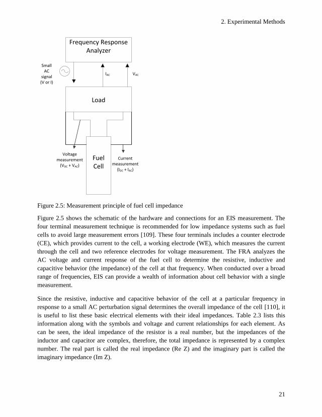
Figure 2.5: Measurement principle of fuel cell impedance
Figure 2.5 shows the schematic of the hardware and connections for an EIS measurement. The
four terminal measurement technique is recommended for low impedance systems such as fuel
cells to avoid large measurement errors [109]. These four terminals includes a counter electrode
(CE), which provides current to the cell, a working electrode (WE), which measures the current
through the cell and two reference electrodes for voltage measurement. The FRA analyzes the
AC voltage and current response of the fuel cell to determine the resistive, inductive and
capacitive behavior (the impedance) of the cell at that frequency. When conducted over a broad
range of frequencies, EIS can provide a wealth of information about cell behavior with a single
measurement.
Since the resistive, inductive and capacitive behavior of the cell at a particular frequency in
response to a small AC perturbation signal determines the overall impedance of the cell [110], it
is useful to list these basic electrical elements with their ideal impedances. Table 2.3 lists this
information along with the symbols and voltage and current relationships for each element. As
can be seen, the ideal impedance of the resistor is a real number, but the impedances of the
inductor and capacitor are complex, therefore, the total impedance is represented by a complex
number. The real part is called the real impedance (Re Z) and the imaginary part is called the
imaginary impedance (Im Z).
2.2. Electrochemical impedance spectroscopy (EIS)
22
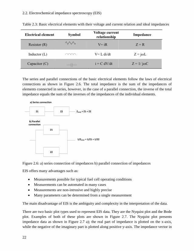
Table 2.3: Basic electrical elements with their voltage and current relation and ideal impedances
Electrical element Symbol Voltage current
relationship Impedance
Resistor (R)
V= iR Z = R
Inductor (L)
V= L di/dt Z = jωL
Capacitor (C)
i = C dV/dt Z = 1/ jωC
The series and parallel connections of the basic electrical elements follow the laws of electrical
connections as shown in Figure 2.6. The total impedance is the sum of the impedances of
elements connected in series, however, in the case of a parallel connection, the inverse of the total
impedance equals the sum of the inverses of the impedances of the individual elements.
Z1 Z2
Z1
Z2
a) Series connection
b) Parallel connection
Ztotal = Z1 + Z2
1/Ztotal = 1/Z1 + 1/Z2
Figure 2.6: a) series connection of impedances b) parallel connection of impedances
EIS offers many advantages such as:
Measurements possible for typical fuel cell operating conditions
Measurements can be automated in many cases
Measurements are non-intrusive and highly precise
Many parameters can be determined from a single measurement
The main disadvantage of EIS is the ambiguity and complexity in the interpretation of the data.
There are two basic plot types used to represent EIS data. They are the Nyquist plot and the Bode
plot. Examples of both of these plots are shown in Figure 2.7. The Nyquist plot presents
impedance data as shown in Figure 2.7 a); the real part of impedance is plotted on the x-axis,
while the negative of the imaginary part is plotted along positive y-axis. The impedance vector in
2. Experimental Methods
23
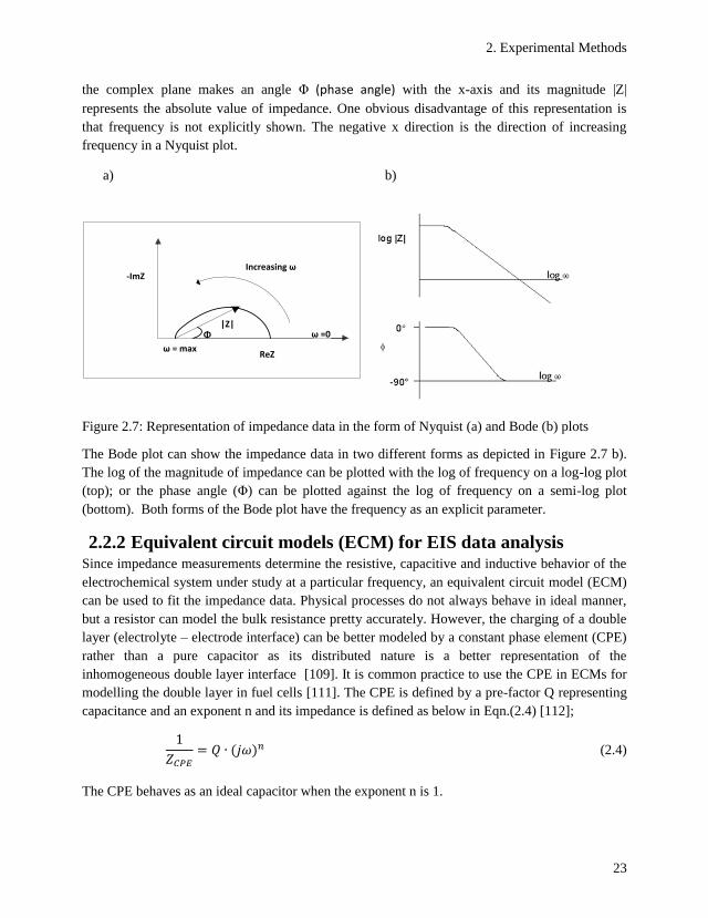
the complex plane makes an angle Φ (phase angle) with the x-axis and its magnitude |Z|
represents the absolute value of impedance. One obvious disadvantage of this representation is
that frequency is not explicitly shown. The negative x direction is the direction of increasing
frequency in a Nyquist plot.
a) b)
-ImZ
ReZ
ω =0
ω = max
|Z|Φ
Increasing ω
Figure 2.7: Representation of impedance data in the form of Nyquist (a) and Bode (b) plots
The Bode plot can show the impedance data in two different forms as depicted in Figure 2.7 b).
The log of the magnitude of impedance can be plotted with the log of frequency on a log-log plot
(top); or the phase angle (Φ) can be plotted against the log of frequency on a semi-log plot
(bottom). Both forms of the Bode plot have the frequency as an explicit parameter.
2.2.2 Equivalent circuit models (ECM) for EIS data analysis Since impedance measurements determine the resistive, capacitive and inductive behavior of the
electrochemical system under study at a particular frequency, an equivalent circuit model (ECM)
can be used to fit the impedance data. Physical processes do not always behave in ideal manner,
but a resistor can model the bulk resistance pretty accurately. However, the charging of a double
layer (electrolyte – electrode interface) can be better modeled by a constant phase element (CPE)
rather than a pure capacitor as its distributed nature is a better representation of the
inhomogeneous double layer interface [109]. It is common practice to use the CPE in ECMs for
modelling the double layer in fuel cells [111]. The CPE is defined by a pre-factor Q representing
capacitance and an exponent n and its impedance is defined as below in Eqn.(2.4) [112];
1
𝑍𝐶𝑃𝐸= 𝑄 ∙ (𝑗𝜔)𝑛 (2.4)
The CPE behaves as an ideal capacitor when the exponent n is 1.
2.2. Electrochemical impedance spectroscopy (EIS)
24
The capacitance of a CPE can be calculated by using the relation from Abouzari et al. [113] or M.
Boudalia et al. [114]. The relation from Abouzari et al. is used in this thesis as shown below in
Eqn.(2.5);
𝐶 = 𝑅1−𝑛
𝑛 ∙ 𝑄1𝑛
(2.5)
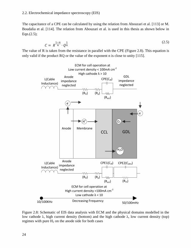
The value of R is taken from the resistance in parallel with the CPE (Figure 2.8). This equation is
only valid if the product RQ or the value of the exponent n is close to unity [115].
Figure 2.8: Schematic of EIS data analysis with ECM and the physical domains modelled in the
low cathode λ, high current density (bottom) and the high cathode λ, low current density (top)
regimes with pure H2 on the anode side for both cases
MembraneCCL GDL
H+
e-
O2
H2O
Anode
e-
Anode impedance neglected
L(Cable Inductance)
(RΩ)
CPE2(Cdlm)
(Rm)(Rp)
(Ract)
CPE1(Cdl)
L(Cable Inductance)
(RΩ) (Rp)(Ract)
CPE(Cdl)Anode
impedance neglected
GDL impedance neglected
ECM for cell operation atLow current density < 100mA cm-2
High cathode λ > 10
ECM for cell operation atHigh current density >100mA cm-2
Low cathode λ < 10
Decreasing Frequency50/100mHz10/100KHz
2. Experimental Methods
25
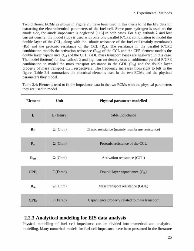
Two different ECMs as shown in Figure 2.8 have been used in this thesis to fit the EIS data for
extracting the electrochemical parameters of the fuel cell. Since pure hydrogen is used on the
anode side, the anode impedance is neglected [116] in both cases. For high cathode λ and low
current density, the model (top) is used with only one parallel R/CPE combination to model the
double layer of the CCL, along with the ohmic resistance of the fuel cell (mainly membrane)
(RΩ) and the protonic resistance of the CCL (Rp). The resistance in the parallel R/CPE
combination models the activation resistance (Ract) of the CCL and the CPE element models the
double layer capacitance (Cdl) of the CCL. GDL mass transport losses are neglected in this case.
The model (bottom) for low cathode λ and high current density uses an additional parallel R/CPE
combination to model the mass transport resistance in the GDL (Rm) and the double layer
property of mass transport Cdl,m respectively. The frequency increases from right to left in the
figure. Table 2.4 summarizes the electrical elements used in the two ECMs and the physical
parameters they model.
Table 2.4: Elements used to fit the impedance data in the two ECMs with the physical parameters
they are used to model
Element Unit Physical parameter modelled
L H (Henry) cable inductance
RΩ Ω (Ohm) Ohmic resistance (mainly membrane resistance)
Rp Ω (Ohm) Protonic resistance of the CCL
Ract Ω (Ohm) Activation resistance (CCL)
CPE1 F (Farad) Double layer capacitance (Cdl)
Rm Ω (Ohm) Mass transport resistance (GDL)
CPE2 F (Farad) Capacitance property related to mass transport
2.2.3 Analytical modeling for EIS data analysis Physical modelling of fuel cell impedance can be divided into numerical and analytical
modelling. Many numerical models for fuel cell impedance have been presented in the literature
2.2. Electrochemical impedance spectroscopy (EIS)
26
[82,117–120] . Using numerical models in least square fitting algorithms for fitting impedance
data is theoretically possible, but it is a very time consuming process due to the need to solve
complex differential equations multiple times numerically. Analytical equations for the CCL
impedance have been derived for the case of fast oxygen transport in [81,121,122]. A simplified
1D analytical model of the CCL impedance has been suggested as a fast and reasonably accurate
alternative to numerical models for sufficiently low current densities by Kulikovsky [83,123].
This model also allows calculating the oxygen diffusivity in the CCL which is a key CCL
transport parameter not readily measureable. This model is described in more detail below and is
used for fitting the low current density impedance of the in-house assembled MEA in this thesis
for a comparison with the fitted electrochemical parameters by ECM modelling.
Mem
bra
ne
CCL
GD
L
ηact
Protonic current
O2
concentration
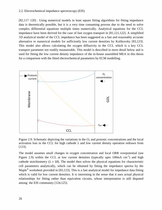
Figure 2.9: Schematic depicting the variations in the O2 and protonic concentrations and the local
activation loss in the CCL for high cathode λ and low current density operation redrawn from
[123].
The model assumes small changes in oxygen concentration and local ORR overpotential (see
Figure 2.9) within the CCL at low current densities (typically upto 100mA cm-2
) and high
cathode stoichiometry (λ > 10). The model then solves the physical equations for characteristic
cell parameters analytically, which can be obtained by fitting the impedance spectra by the
Maple®
worksheet provided in [83,123]. This is a fast analytical model for impedance data fitting
which is valid for low current densities. It is interesting in the sense that it uses actual physical
relationships for fitting rather than equivalent circuits, whose interpretation is still disputed
among the EIS community [124,125].
2. Experimental Methods
27
The basic nomenclature followed by this 1D analytical model (called AM from here on for
brevity) is as follows;
b = Tafel slope (V)
lt = CCL thickness (cm)
σp = Protonic conductivity of the CCL (Ω-1 cm
-1)
j0 = Current density (A cm-2
)
F = Faraday’s constant (C mol-1
)
Doxp = Diffusion constant of oxygen in the CCL (cm2 s
-1)
Cref = Reference oxygen concentration (mol cm-3
)
Rp = Protonic resistance of CCL (Ω cm2)
Ract = Activation resistance of the CCL (Ω cm2)
Roxp = Oxygen transport resistance of the CCL (Ω cm2)
Cdl = Volumetric double layer capacitance (F cm-3
)
The values of j0, F, Cref and lt are known in our case (lt is 0.012 cm for the in-house assembled
MEA). The Maple®
worksheet implementing the analytical model calculates the values of b, σp,
Cdl and Doxp analytically by fitting the impedance data. The characteristic fuel cell resistances are
then calculated by using the Eqns. (2.6) to (2.8) below;
𝑅𝑝 =𝑙𝑡
3σ𝑝 (2.6)
𝑅𝑎𝑐𝑡 = 𝑏
𝑗0 (2.7)
𝑅𝑜𝑥𝑝 = 𝑏 𝑙𝑡
3(4𝐹𝐷𝐶𝑟𝑒𝑓) (2.8)
The double layer capacitance is calculated according to Eqn. (2.9);
𝐶𝑑𝑙 = 1
𝜔∗𝑅𝑎𝑐𝑡 (2.9)
2.2. Electrochemical impedance spectroscopy (EIS)
28
Where 𝜔∗ is the angular frequency at the peak value of negative imaginary impedance (top of the
semi arc in the Nyquist plot) in radians per second with the conversion from the regular
frequency (f) in Hertz (Hz) is as in Eqn. (2.10);
𝜔 = 2𝜋𝑓 (2.10)
The impedance data needs to be entered into the Maple worksheet along with initial guesses for
each of the parameters to be calculated. It is essential to use reasonable initial guesses otherwise
the solution may not converge.
The AM does not explicitly calculate the ohmic resistance RΩ, but it can be obtained from the left
intercept of the Nyquist plot. The AM instead calculates the mass transport resistance of the CCL
Roxp (indirectly) based on the value of the diffusion coefficient of oxygen inside the CCL (Doxp).
This is a parameter not provided by the ECM. In fact, another parameter Db, the diffusion
coefficient of oxygen in the GDL can also be calculated by the AM for sufficiently thin CCLs
(around 40µm which is typical for LT-PEFC) but the actual used CCL in this thesis is much too
thick (120µm) therefore the value of Db is not realistic and thus not used. These two parameters
are of very high practical importance and methods for their accurate determination are scarce in
the literature.
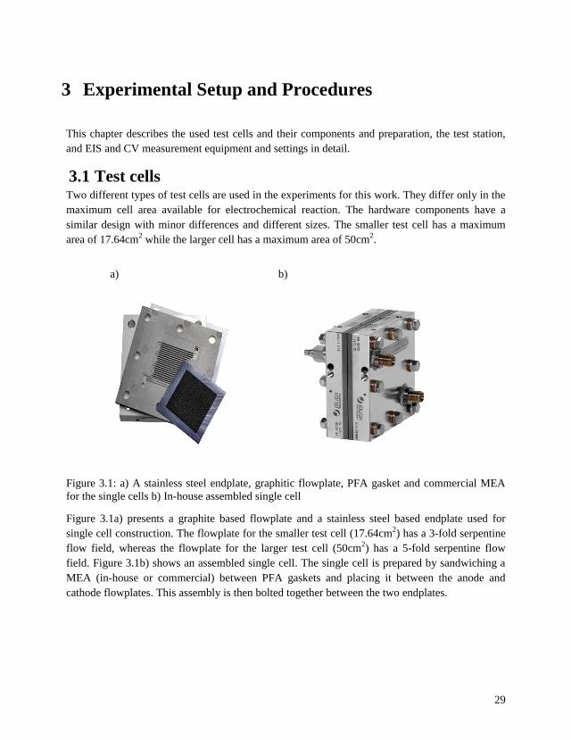
29
3 Experimental Setup and Procedures
This chapter describes the used test cells and their components and preparation, the test station,
and EIS and CV measurement equipment and settings in detail.
3.1 Test cells Two different types of test cells are used in the experiments for this work. They differ only in the
maximum cell area available for electrochemical reaction. The hardware components have a
similar design with minor differences and different sizes. The smaller test cell has a maximum
area of 17.64cm2 while the larger cell has a maximum area of 50cm
2.
Figure 3.1: a) A stainless steel endplate, graphitic flowplate, PFA gasket and commercial MEA
for the single cells b) In-house assembled single cell
Figure 3.1a) presents a graphite based flowplate and a stainless steel based endplate used for
single cell construction. The flowplate for the smaller test cell (17.64cm2) has a 3-fold serpentine
flow field, whereas the flowplate for the larger test cell (50cm2) has a 5-fold serpentine flow
field. Figure 3.1b) shows an assembled single cell. The single cell is prepared by sandwiching a
MEA (in-house or commercial) between PFA gaskets and placing it between the anode and
cathode flowplates. This assembly is then bolted together between the two endplates.
a) b)
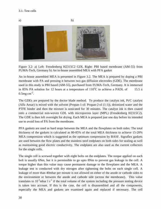
3.1. Test cells
30
a) b)
Figure 3.2: a) Left: Freudenberg H2315C2 GDL Right: PBI based membrane (AM-55) from
FUMA-Tech, Germany b) An in-house assembled MEA with PFA gasket
An in-house assembled MEA is presented in Figure 3.2. The MEA is prepared by doping a PBI
membrane with PA and pressing it between two gas diffusion electrodes (GDE). The membrane
used in this study is PBI based (AM-55), purchased from FUMA-Tech, Germany. It is immersed
in 85% PA solution for 12 hours at a temperature of 110oC to achieve a PADL of 15.5 ±
0.5mg cm-2
.
The GDEs are prepared by the doctor blade method. To produce the catalyst ink, Pt/C catalyst
(Alfa Aesar) is mixed with the solvent (Propan-1-ol: Propan-2-ol (1:1)), deionized water and the
PTFE binder and then the mixture is sonicated for 30 minutes. The catalyst ink is then coated
onto a commercial non-woven GDL with microporous layer (MPL) (Freudenberg H2315C2).
The GDE is then left overnight for drying. Each MEA is prepared just one day before its intended
use to avoid loss of PA from the membrane.
PFA gaskets are used as hard stops between the MEA and the flowplates on both sides. The total
thickness of the gaskets is calculated as 80-85% of the total MEA thickness to achieve 15-20%
MEA compression which is suggested as the optimum compression by BASF. Sigraflex gaskets
are used between the flow plates and the stainless steel endplates on both sides for sealing as well
as maintaining good electric conductivity. The endplates are also used as the current collectors
for the single cells.
The single cell is screwed together with eight bolts on the endplates. The torque applied on each
bolt is usually 6Nm, but it is permissible to go upto 8Nm to prevent gas leakage in the cell. A
torque higher than this value may cause permanent damage to the flowplates and the MEA. A
leakage test is conducted with dry nitrogen after tightening the bolts on each single cell. A
leakage of more than 40mbar per minute is not allowed on either of the anode or cathode sides to
the environment or between the anode and cathode side (across the membrane). This value
translates to 10-3
mbar l s-1
if the total volume of the system including the pressure testing device
is taken into account. If this is the case, the cell is disassembled and all the components,
especially the MEA and gaskets are examined again and replaced if necessary. The cell
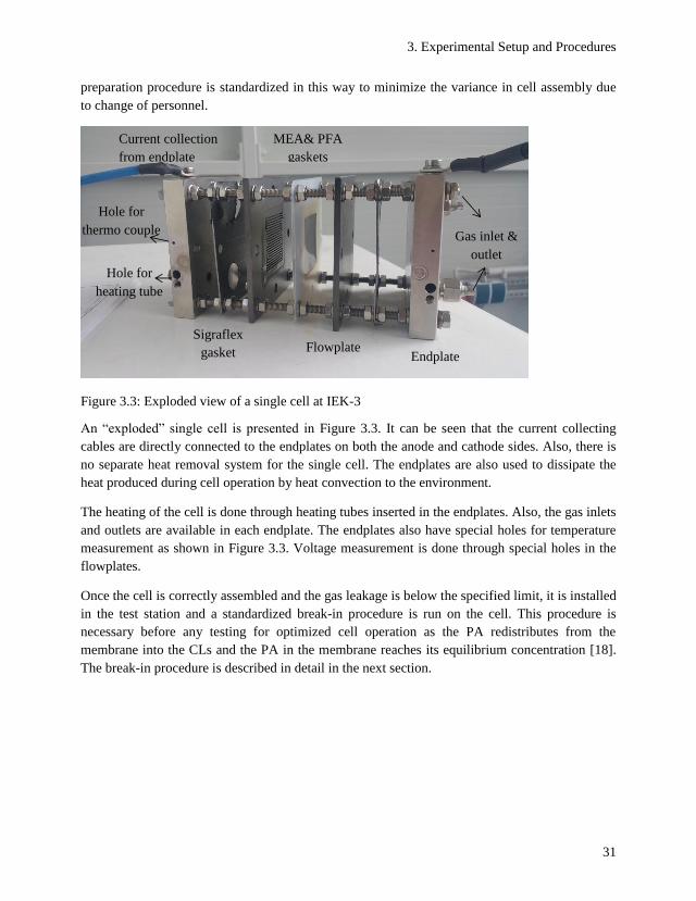
3. Experimental Setup and Procedures
31
preparation procedure is standardized in this way to minimize the variance in cell assembly due
to change of personnel.
Figure 3.3: Exploded view of a single cell at IEK-3
An “exploded” single cell is presented in Figure 3.3. It can be seen that the current collecting
cables are directly connected to the endplates on both the anode and cathode sides. Also, there is
no separate heat removal system for the single cell. The endplates are also used to dissipate the
heat produced during cell operation by heat convection to the environment.
The heating of the cell is done through heating tubes inserted in the endplates. Also, the gas inlets
and outlets are available in each endplate. The endplates also have special holes for temperature
measurement as shown in Figure 3.3. Voltage measurement is done through special holes in the
flowplates.
Once the cell is correctly assembled and the gas leakage is below the specified limit, it is installed
in the test station and a standardized break-in procedure is run on the cell. This procedure is
necessary before any testing for optimized cell operation as the PA redistributes from the
membrane into the CLs and the PA in the membrane reaches its equilibrium concentration [18].
The break-in procedure is described in detail in the next section.
MEA& PFA
gaskets
Sigraflex
gasket Flowplate Endplate
Current collection
from endplate
Hole for
heating tube
Hole for
thermo couple Gas inlet &
outlet
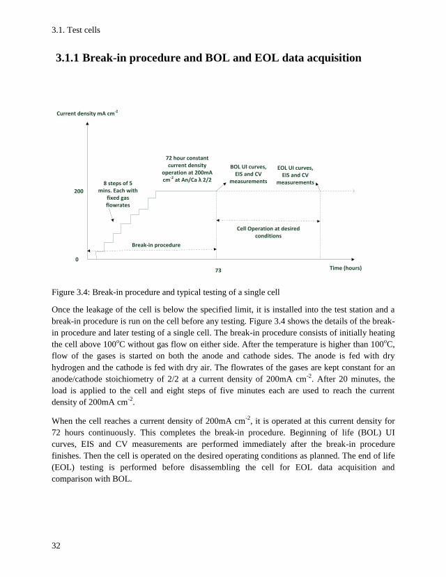
3.1. Test cells
32
3.1.1 Break-in procedure and BOL and EOL data acquisition
Current density mA cm-2
72 hour constant current density
operation at 200mA cm-2 at An/Ca λ 2/2
EOL UI curves, EIS and CV
measurements
Break-in procedure
Cell Operation at desired conditions
Time (hours)73
200
0
8 steps of 5 mins. Each with
fixed gas flowrates
BOL UI curves, EIS and CV
measurements
Figure 3.4: Break-in procedure and typical testing of a single cell
Once the leakage of the cell is below the specified limit, it is installed into the test station and a
break-in procedure is run on the cell before any testing. Figure 3.4 shows the details of the break-
in procedure and later testing of a single cell. The break-in procedure consists of initially heating
the cell above 100oC without gas flow on either side. After the temperature is higher than 100
oC,
flow of the gases is started on both the anode and cathode sides. The anode is fed with dry
hydrogen and the cathode is fed with dry air. The flowrates of the gases are kept constant for an
anode/cathode stoichiometry of 2/2 at a current density of 200mA cm-2
. After 20 minutes, the
load is applied to the cell and eight steps of five minutes each are used to reach the current
density of 200mA cm-2
.
When the cell reaches a current density of 200mA cm-2
, it is operated at this current density for
72 hours continuously. This completes the break-in procedure. Beginning of life (BOL) UI
curves, EIS and CV measurements are performed immediately after the break-in procedure
finishes. Then the cell is operated on the desired operating conditions as planned. The end of life
(EOL) testing is performed before disassembling the cell for EOL data acquisition and
comparison with BOL.
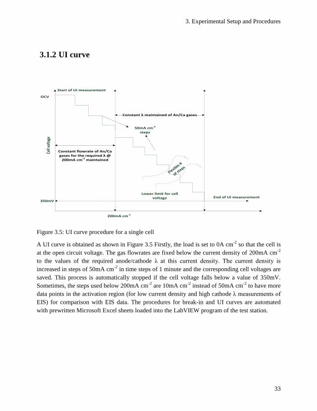
3. Experimental Setup and Procedures
33
3.1.2 UI curve
200mA cm-2
Cell
volta
ge
OCV
350mV
Constant λ maintained of An/Ca gases
50mA cm-2 steps
End of UI measurementLower limit for cell
voltage
Constant flowrate of An/Ca gases for the required λ @
200mA cm-2 maintained
Start of UI measurement
Flexible #
of ste
ps
Figure 3.5: UI curve procedure for a single cell
A UI curve is obtained as shown in Figure 3.5 Firstly, the load is set to 0A cm-2
so that the cell is
at the open circuit voltage. The gas flowrates are fixed below the current density of 200mA cm-2
to the values of the required anode/cathode λ at this current density. The current density is
increased in steps of 50mA cm-2
in time steps of 1 minute and the corresponding cell voltages are
saved. This process is automatically stopped if the cell voltage falls below a value of 350mV.
Sometimes, the steps used below 200mA cm-2
are 10mA cm-2
instead of 50mA cm-2
to have more
data points in the activation region (for low current density and high cathode λ measurements of
EIS) for comparison with EIS data. The procedures for break-in and UI curves are automated
with prewritten Microsoft Excel sheets loaded into the LabVIEW program of the test station.
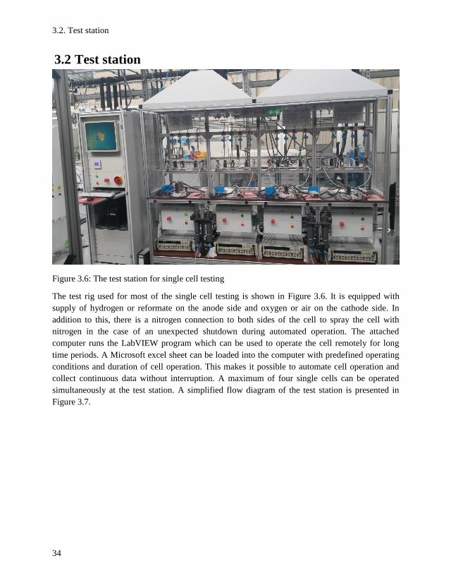
3.2. Test station
34
3.2 Test station
Figure 3.6: The test station for single cell testing
The test rig used for most of the single cell testing is shown in Figure 3.6. It is equipped with
supply of hydrogen or reformate on the anode side and oxygen or air on the cathode side. In
addition to this, there is a nitrogen connection to both sides of the cell to spray the cell with
nitrogen in the case of an unexpected shutdown during automated operation. The attached
computer runs the LabVIEW program which can be used to operate the cell remotely for long
time periods. A Microsoft excel sheet can be loaded into the computer with predefined operating
conditions and duration of cell operation. This makes it possible to automate cell operation and
collect continuous data without interruption. A maximum of four single cells can be operated
simultaneously at the test station. A simplified flow diagram of the test station is presented in
Figure 3.7.
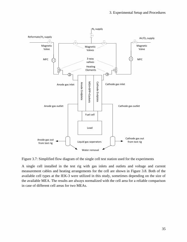
3. Experimental Setup and Procedures
35
An
od
e End
plate
Cath
od
e End
plate
M
EA+B
PP
+Gaskets
Load
Fuel cell
Anode gas inlet
Anode gas outlet Cathode gas outlet
Cathode gas inlet
Liquid gas seperatorsAnode gas outfrom test rig
Cathode gas out from test rig
Water removal
Air/O2 supplyReformate/H2 supply
N2 supply
Heating Elements
3-way vallves
MFCMFC
Magnetic Valves
Magnetic Valve
Magnetic Valve
Figure 3.7: Simplified flow diagram of the single cell test station used for the experiments
A single cell installed in the test rig with gas inlets and outlets and voltage and current
measurement cables and heating arrangements for the cell are shown in Figure 3.8. Both of the
available cell types at the IEK-3 were utilized in this study, sometimes depending on the size of
the available MEA. The results are always normalized with the cell area for a reliable comparison
in case of different cell areas for two MEAs.
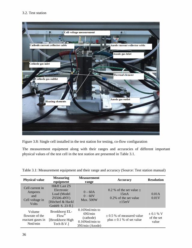
3.2. Test station
36
Figure 3.8: Single cell installed in the test station for testing, co-flow configuration
The measurement equipment along with their ranges and accuracies of different important
physical values of the test cell in the test station are presented in Table 3.1.
Table 3.1: Measurement equipment and their range and accuracy (Source: Test station manual)
Physical value Measuring
equipment
Measurement
range Accuracy Resolution
Cell current in
Amperes
and
Cell voltage in
Volts
H&H Last ZS
Electronic
Load (Model
ZS506-4NV)
[Höcherl & Hackl
GmbH: S. 23 ff.]
0 – 60A
0 – 60V
Max. 500W
0.2 % of the set value ±
15mA
0.2% of the set value
±15mV
0.01A
0.01V
Volume
flowrate of the
reactant gases in
Nml/min
Bronkhorst EL-
Flow®
[Bronkhorst High
Tech B.V.]
0.16Nml/min to
6Nl/min
(cathode)
0.16Nml/min to
3Nl/min (Anode)
± 0.5 % of measured value
plus ± 0.1 % of set value
± 0.1 % V
of the set
value
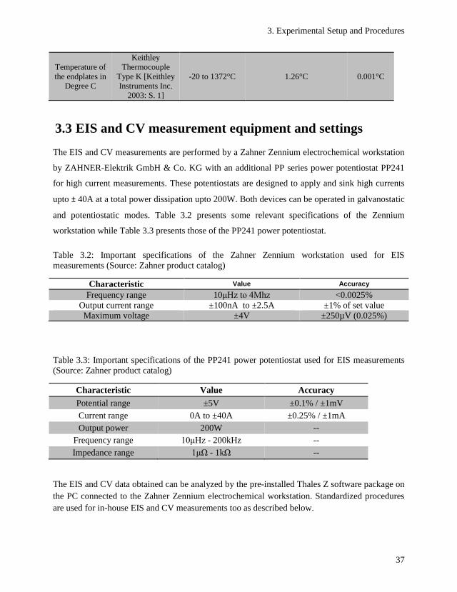
3. Experimental Setup and Procedures
37
Temperature of
the endplates in
Degree C
Keithley
Thermocouple
Type K [Keithley
Instruments Inc.
2003: S. 1]
-20 to 1372°C 1.26°C 0.001°C
3.3 EIS and CV measurement equipment and settings
The EIS and CV measurements are performed by a Zahner Zennium electrochemical workstation
by ZAHNER-Elektrik GmbH & Co. KG with an additional PP series power potentiostat PP241
for high current measurements. These potentiostats are designed to apply and sink high currents
upto ± 40A at a total power dissipation upto 200W. Both devices can be operated in galvanostatic
and potentiostatic modes. Table 3.2 presents some relevant specifications of the Zennium
workstation while Table 3.3 presents those of the PP241 power potentiostat.
Table 3.2: Important specifications of the Zahner Zennium workstation used for EIS
measurements (Source: Zahner product catalog)
Characteristic Value Accuracy
Frequency range 10μHz to 4Mhz <0.0025%
Output current range ±100nA to ±2.5A ±1% of set value
Maximum voltage ±4V ±250µV (0.025%)
Table 3.3: Important specifications of the PP241 power potentiostat used for EIS measurements
(Source: Zahner product catalog)
Characteristic Value Accuracy
Potential range ±5V ±0.1% / ±1mV
Current range 0A to ±40A ±0.25% / ±1mA
Output power 200W --
Frequency range 10μHz - 200kHz --
Impedance range 1μΩ - 1kΩ --
The EIS and CV data obtained can be analyzed by the pre-installed Thales Z software package on
the PC connected to the Zahner Zennium electrochemical workstation. Standardized procedures
are used for in-house EIS and CV measurements too as described below.
3.3. EIS and CV measurement equipment and settings
38
3.3.1 EIS measurements
EIS is used to obtain impedance measurements for different cells at different operating
conditions. The setup for the EIS measurements consists of a conventional two-electrode setup
with the anode serving as a quasi-reference and counter electrode and the cathode serving as the
working electrode. A frequency range of 10-1
– 105Hz and AC signal voltage amplitude of
± 10mV is usually chosen in this study; however a minimum frequency of 50mHz is also chosen
at times when higher resolution is required at the low frequency end of the impedance spectrum.
Other important parameters which must be selected include measurement points to be recorded
per decade of frequency (steps per decade) and measure periods for each EIS measurement. For
each of these parameters, two values must be given, one below 66Hz and the other above this
frequency. This enables optimization of resolution over measuring time and accuracy over
measuring time since measuring time is dominant below the frequency of 66Hz. In this thesis,
four measure points per decade are used below 66Hz for both of these parameters and ten
measure points per decade are used above 66Hz. Also, four measure periods are selected below
66Hz and ten measure periods above 66Hz. These settings are used for all the measurements
unless otherwise stated. This helps achieve better reproducibility and comparable results as well
as optimization of the measuring time for each EIS measurement while maintaining reasonable
accuracy. Care is taken to measure impedance at stationary conditions for reliable measurements.
The fuel cell is first run on the required conditions for at least five minutes and then the
impedance measurement is started. The cables connecting the Zennium workstation to the cell are
twisted together properly to minimize cable inductance and noise. Each measurement is repeated
at least once for comparison of the reproducibility and backup of the impedance spectra.
3.3.2 CV measurements The Zahner Zennium electrochemical workstation is also used for the CV measurements. The CV
measurements are done in potentiostatic mode. In order to perform the measurement, the fuel cell
is fed with dry hydrogen (70Nml min-1
) and dry nitrogen (100Nml min-1
) at the anode and
cathode sides respectively. The anode works as pseudo-reference and counter electrode, while the
cathode is the working electrode. The potential of the working electrode is scanned between
0.05Vand 1.2V with a scan rate of 50mV s-1
and four cycles are performed. The CV data is
analyzed using the Thales Z CV software. The cathode catalyst active area is estimated
considering the positive current density peak related to hydrogen desorption for the last cycle.
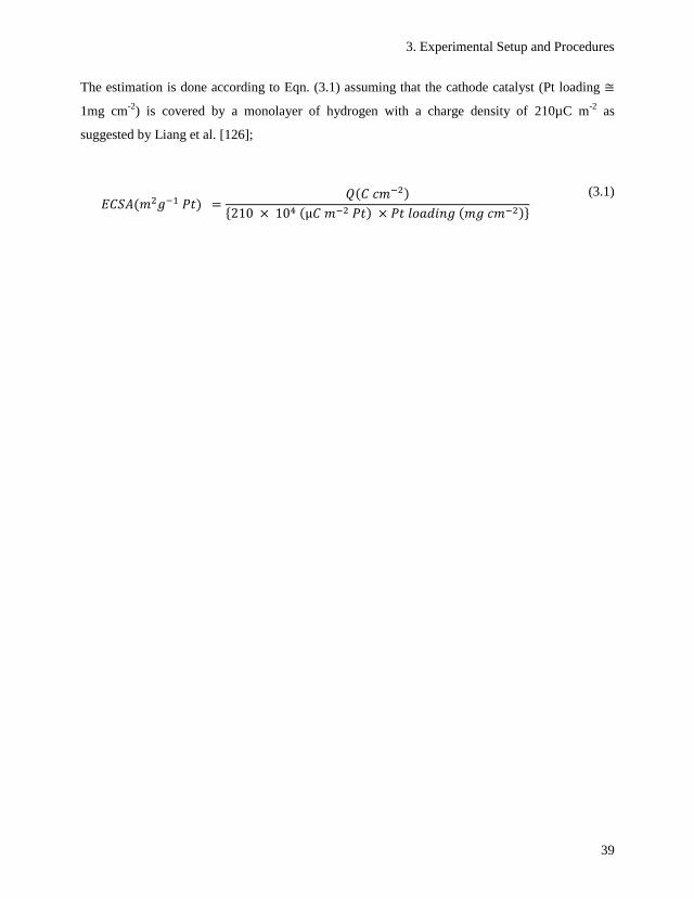
3. Experimental Setup and Procedures
39
The estimation is done according to Eqn. (3.1) assuming that the cathode catalyst (Pt loading ≅
1mg cm-2
) is covered by a monolayer of hydrogen with a charge density of 210µC m-2
as
suggested by Liang et al. [126];
𝐸𝐶𝑆𝐴(𝑚2𝑔−1 𝑃𝑡) =𝑄(𝐶 𝑐𝑚−2)
210 × 104 (µ𝐶 𝑚−2 𝑃𝑡) × 𝑃𝑡 𝑙𝑜𝑎𝑑𝑖𝑛𝑔 (𝑚𝑔 𝑐𝑚−2)
(3.1)

3.3. EIS and CV measurement equipment and settings
40
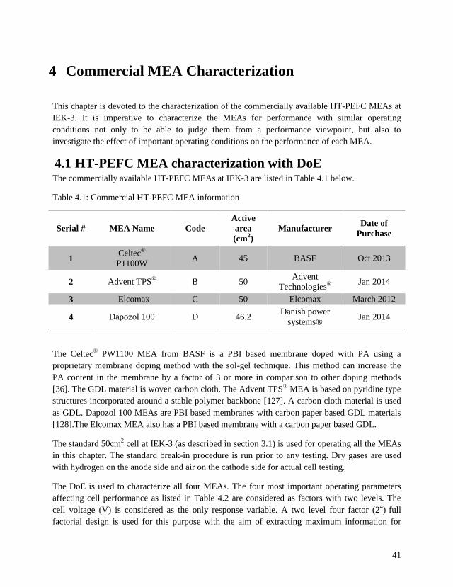
41
4 Commercial MEA Characterization
This chapter is devoted to the characterization of the commercially available HT-PEFC MEAs at
IEK-3. It is imperative to characterize the MEAs for performance with similar operating
conditions not only to be able to judge them from a performance viewpoint, but also to
investigate the effect of important operating conditions on the performance of each MEA.
4.1 HT-PEFC MEA characterization with DoE The commercially available HT-PEFC MEAs at IEK-3 are listed in Table 4.1 below.
Table 4.1: Commercial HT-PEFC MEA information
Serial # MEA Name Code
Active
area
(cm2)
Manufacturer Date of
Purchase
1 Celtec
®
P1100W A 45 BASF Oct 2013
2 Advent TPS®
B 50 Advent
Technologies®
Jan 2014
3 Elcomax C 50 Elcomax March 2012
4 Dapozol 100 D 46.2 Danish power
systems® Jan 2014
The Celtec®
PW1100 MEA from BASF is a PBI based membrane doped with PA using a
proprietary membrane doping method with the sol-gel technique. This method can increase the
PA content in the membrane by a factor of 3 or more in comparison to other doping methods
[36]. The GDL material is woven carbon cloth. The Advent TPS®
MEA is based on pyridine type
structures incorporated around a stable polymer backbone [127]. A carbon cloth material is used
as GDL. Dapozol 100 MEAs are PBI based membranes with carbon paper based GDL materials
[128].The Elcomax MEA also has a PBI based membrane with a carbon paper based GDL.
The standard 50cm2 cell at IEK-3 (as described in section 3.1) is used for operating all the MEAs
in this chapter. The standard break-in procedure is run prior to any testing. Dry gases are used
with hydrogen on the anode side and air on the cathode side for actual cell testing.
The DoE is used to characterize all four MEAs. The four most important operating parameters
affecting cell performance as listed in Table 4.2 are considered as factors with two levels. The
cell voltage (V) is considered as the only response variable. A two level four factor (24) full
factorial design is used for this purpose with the aim of extracting maximum information for
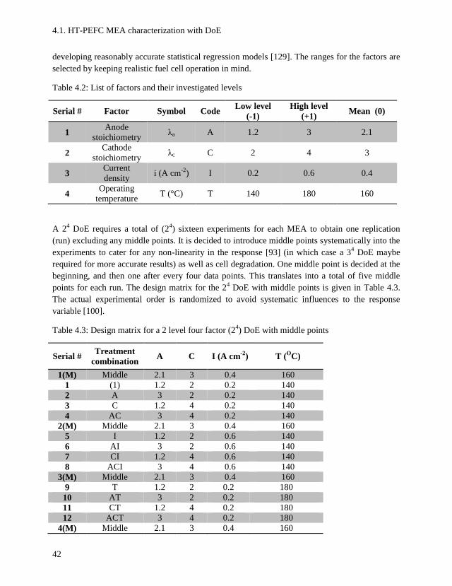
4.1. HT-PEFC MEA characterization with DoE
42
developing reasonably accurate statistical regression models [129]. The ranges for the factors are
selected by keeping realistic fuel cell operation in mind.
Table 4.2: List of factors and their investigated levels
Serial # Factor Symbol Code Low level
(-1)
High level
(+1) Mean (0)
1 Anode
stoichiometry λa A 1.2 3 2.1
2 Cathode
stoichiometry λc C 2 4 3
3 Current
density i (A cm
-2) I 0.2 0.6 0.4
4 Operating
temperature T (°C) T 140 180 160
A 24 DoE requires a total of (2
4) sixteen experiments for each MEA to obtain one replication
(run) excluding any middle points. It is decided to introduce middle points systematically into the
experiments to cater for any non-linearity in the response [93] (in which case a 34 DoE maybe
required for more accurate results) as well as cell degradation. One middle point is decided at the
beginning, and then one after every four data points. This translates into a total of five middle
points for each run. The design matrix for the 24 DoE with middle points is given in Table 4.3.
The actual experimental order is randomized to avoid systematic influences to the response
variable [100].
Table 4.3: Design matrix for a 2 level four factor (24) DoE with middle points
Serial # Treatment
combination A C I (A cm
-2) T (
OC)
1(M) Middle 2.1 3 0.4 160
1 (1) 1.2 2 0.2 140
2 A 3 2 0.2 140
3 C 1.2 4 0.2 140
4 AC 3 4 0.2 140
2(M) Middle 2.1 3 0.4 160
5 I 1.2 2 0.6 140
6 AI 3 2 0.6 140
7 CI 1.2 4 0.6 140
8 ACI 3 4 0.6 140
3(M) Middle 2.1 3 0.4 160
9 T 1.2 2 0.2 180
10 AT 3 2 0.2 180
11 CT 1.2 4 0.2 180
12 ACT 3 4 0.2 180
4(M) Middle 2.1 3 0.4 160
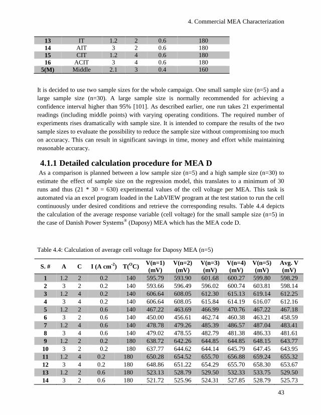
4. Commercial MEA Characterization
43
13 IT 1.2 2 0.6 180
14 AIT 3 2 0.6 180
15 CIT 1.2 4 0.6 180
16 ACIT 3 4 0.6 180
5(M) Middle 2.1 3 0.4 160
It is decided to use two sample sizes for the whole campaign. One small sample size (n=5) and a
large sample size (n=30). A large sample size is normally recommended for achieving a
confidence interval higher than 95% [101]. As described earlier, one run takes 21 experimental
readings (including middle points) with varying operating conditions. The required number of
experiments rises dramatically with sample size. It is intended to compare the results of the two
sample sizes to evaluate the possibility to reduce the sample size without compromising too much
on accuracy. This can result in significant savings in time, money and effort while maintaining
reasonable accuracy.
4.1.1 Detailed calculation procedure for MEA D As a comparison is planned between a low sample size (n=5) and a high sample size (n=30) to
estimate the effect of sample size on the regression model, this translates to a minimum of 30
runs and thus (21 * 30 = 630) experimental values of the cell voltage per MEA. This task is
automated via an excel program loaded in the LabVIEW program at the test station to run the cell
continuously under desired conditions and retrieve the corresponding results. Table 4.4 depicts
the calculation of the average response variable (cell voltage) for the small sample size (n=5) in
the case of Danish Power Systems®
(Daposy) MEA which has the MEA code D.
Table 4.4: Calculation of average cell voltage for Daposy MEA (n=5)
S. # A C I (A cm-2
) T(O
C) V(n=1)
(mV)
V(n=2)
(mV)
V(n=3)
(mV)
V(n=4)
(mV)
V(n=5)
(mV)
Avg. V
(mV)
1 1.2 2 0.2 140 595.79 593.90 601.68 600.27 599.80 598.29
2 3 2 0.2 140 593.66 596.49 596.02 600.74 603.81 598.14
3 1.2 4 0.2 140 606.64 608.05 612.30 615.13 619.14 612.25
4 3 4 0.2 140 606.64 608.05 615.84 614.19 616.07 612.16
5 1.2 2 0.6 140 467.22 463.69 466.99 470.76 467.22 467.18
6 3 2 0.6 140 450.00 456.61 462.74 460.38 463.21 458.59
7 1.2 4 0.6 140 478.78 479.26 485.39 486.57 487.04 483.41
8 3 4 0.6 140 479.02 478.55 482.79 481.38 486.33 481.61
9 1.2 2 0.2 180 638.72 642.26 644.85 644.85 648.15 643.77
10 3 2 0.2 180 637.77 644.62 644.14 645.79 647.45 643.95
11 1.2 4 0.2 180 650.28 654.52 655.70 656.88 659.24 655.32
12 3 4 0.2 180 648.86 651.22 654.29 655.70 658.30 653.67
13 1.2 2 0.6 180 523.13 528.79 529.50 532.33 533.75 529.50
14 3 2 0.6 180 521.72 525.96 524.31 527.85 528.79 525.73
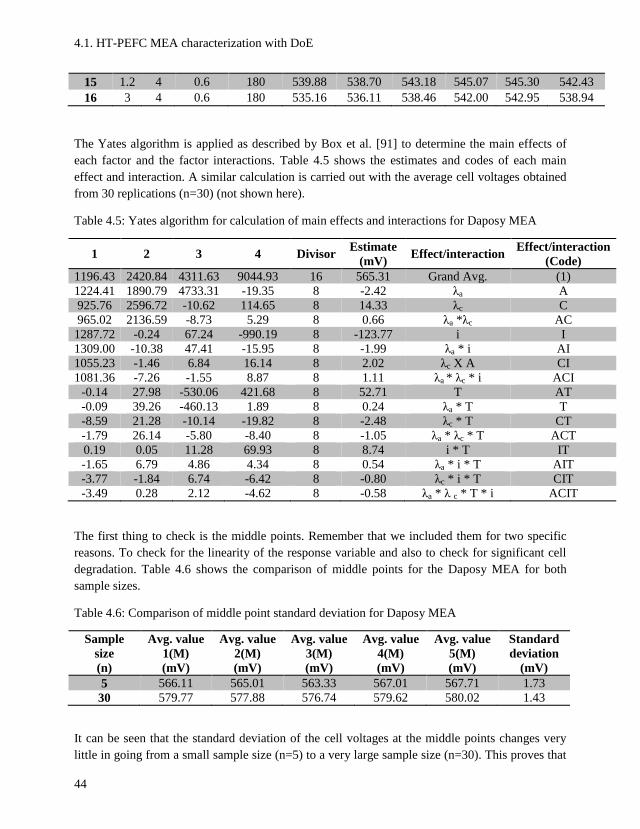
4.1. HT-PEFC MEA characterization with DoE
44
15 1.2 4 0.6 180 539.88 538.70 543.18 545.07 545.30 542.43
16 3 4 0.6 180 535.16 536.11 538.46 542.00 542.95 538.94
The Yates algorithm is applied as described by Box et al. [91] to determine the main effects of
each factor and the factor interactions. Table 4.5 shows the estimates and codes of each main
effect and interaction. A similar calculation is carried out with the average cell voltages obtained
from 30 replications (n=30) (not shown here).
Table 4.5: Yates algorithm for calculation of main effects and interactions for Daposy MEA
1 2 3 4 Divisor Estimate
(mV) Effect/interaction
Effect/interaction
(Code)
1196.43 2420.84 4311.63 9044.93 16 565.31 Grand Avg. (1)
1224.41 1890.79 4733.31 -19.35 8 -2.42 λa A
925.76 2596.72 -10.62 114.65 8 14.33 λc C
965.02 2136.59 -8.73 5.29 8 0.66 λa *λc AC
1287.72 -0.24 67.24 -990.19 8 -123.77 i I
1309.00 -10.38 47.41 -15.95 8 -1.99 λa * i AI
1055.23 -1.46 6.84 16.14 8 2.02 λc X A CI
1081.36 -7.26 -1.55 8.87 8 1.11 λa * λc * i ACI
-0.14 27.98 -530.06 421.68 8 52.71 T AT
-0.09 39.26 -460.13 1.89 8 0.24 λa * T T
-8.59 21.28 -10.14 -19.82 8 -2.48 λc * T CT
-1.79 26.14 -5.80 -8.40 8 -1.05 λa * λc * T ACT
0.19 0.05 11.28 69.93 8 8.74 i * T IT
-1.65 6.79 4.86 4.34 8 0.54 λa * i * T AIT
-3.77 -1.84 6.74 -6.42 8 -0.80 λc * i * T CIT
-3.49 0.28 2.12 -4.62 8 -0.58 λa * λ c * T * i ACIT
The first thing to check is the middle points. Remember that we included them for two specific
reasons. To check for the linearity of the response variable and also to check for significant cell
degradation. Table 4.6 shows the comparison of middle points for the Daposy MEA for both
sample sizes.
Table 4.6: Comparison of middle point standard deviation for Daposy MEA
Sample
size
(n)
Avg. value
1(M)
(mV)
Avg. value
2(M)
(mV)
Avg. value
3(M)
(mV)
Avg. value
4(M)
(mV)
Avg. value
5(M)
(mV)
Standard
deviation
(mV)
5 566.11 565.01 563.33 567.01 567.71 1.73
30 579.77 577.88 576.74 579.62 580.02 1.43
It can be seen that the standard deviation of the cell voltages at the middle points changes very
little in going from a small sample size (n=5) to a very large sample size (n=30). This proves that
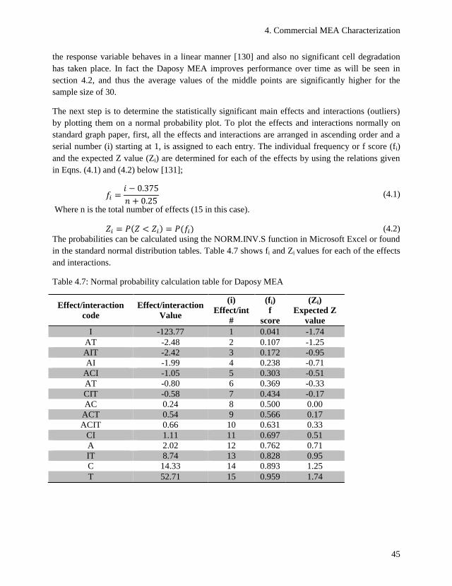
4. Commercial MEA Characterization
45
the response variable behaves in a linear manner [130] and also no significant cell degradation
has taken place. In fact the Daposy MEA improves performance over time as will be seen in
section 4.2, and thus the average values of the middle points are significantly higher for the
sample size of 30.
The next step is to determine the statistically significant main effects and interactions (outliers)
by plotting them on a normal probability plot. To plot the effects and interactions normally on
standard graph paper, first, all the effects and interactions are arranged in ascending order and a
serial number (i) starting at 1, is assigned to each entry. The individual frequency or f score (fi)
and the expected Z value (Zi) are determined for each of the effects by using the relations given
in Eqns. (4.1) and (4.2) below [131];
𝑓𝑖 =𝑖 − 0.375
𝑛 + 0.25 (4.1)
Where n is the total number of effects (15 in this case).
𝑍𝑖 = 𝑃(𝑍 < 𝑍𝑖) = 𝑃(𝑓𝑖) (4.2)
The probabilities can be calculated using the NORM.INV.S function in Microsoft Excel or found
in the standard normal distribution tables. Table 4.7 shows fi and Zi values for each of the effects
and interactions.
Table 4.7: Normal probability calculation table for Daposy MEA
Effect/interaction
code
Effect/interaction
Value
(i)
Effect/int
#
(fi)
f
score
(Zi)
Expected Z
value
I -123.77 1 0.041 -1.74
AT -2.48 2 0.107 -1.25
AIT -2.42 3 0.172 -0.95
AI -1.99 4 0.238 -0.71
ACI -1.05 5 0.303 -0.51
AT -0.80 6 0.369 -0.33
CIT -0.58 7 0.434 -0.17
AC 0.24 8 0.500 0.00
ACT 0.54 9 0.566 0.17
ACIT 0.66 10 0.631 0.33
CI 1.11 11 0.697 0.51
A 2.02 12 0.762 0.71
IT 8.74 13 0.828 0.95
C 14.33 14 0.893 1.25
T 52.71 15 0.959 1.74
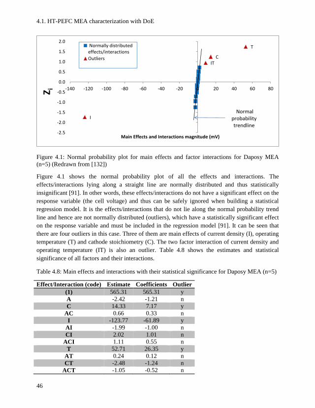
4.1. HT-PEFC MEA characterization with DoE
46
Figure 4.1: Normal probability plot for main effects and factor interactions for Daposy MEA
(n=5) (Redrawn from [132])
Figure 4.1 shows the normal probability plot of all the effects and interactions. The
effects/interactions lying along a straight line are normally distributed and thus statistically
insignificant [91]. In other words, these effects/interactions do not have a significant effect on the
response variable (the cell voltage) and thus can be safely ignored when building a statistical
regression model. It is the effects/interactions that do not lie along the normal probability trend
line and hence are not normally distributed (outliers), which have a statistically significant effect
on the response variable and must be included in the regression model [91]. It can be seen that
there are four outliers in this case. Three of them are main effects of current density (I), operating
temperature (T) and cathode stoichiometry (C). The two factor interaction of current density and
operating temperature (IT) is also an outlier. Table 4.8 shows the estimates and statistical
significance of all factors and their interactions.
Table 4.8: Main effects and interactions with their statistical significance for Daposy MEA (n=5)
Effect/Interaction (code) Estimate Coefficients Outlier
(1) 565.31 565.31 y
A -2.42 -1.21 n
C 14.33 7.17 y
AC 0.66 0.33 n
I -123.77 -61.89 y
AI -1.99 -1.00 n
CI 2.02 1.01 n
ACI 1.11 0.55 n
T 52.71 26.35 y
AT 0.24 0.12 n
CT -2.48 -1.24 n
ACT -1.05 -0.52 n
I
IT C
T
-2.5
-2.0
-1.5
-1.0
-0.5
0.0
0.5
1.0
1.5
2.0
-140 -120 -100 -80 -60 -40 -20 0 20 40 60 80Z i
Main Effects and Interactions magnitude (mV)
Normally distributedeffects/interactions
Outliers
Normal probability trendline

4. Commercial MEA Characterization
47
IT 8.74 4.37 y
AIT 0.54 0.27 n
CIT -0.80 -0.40 n
ACIT -0.58 -0.29 n
The final task is to develop the statistical regression models based upon the outliers. A
transformation of each factor range to a scale of -1 to 1 is used for this purpose, which is given in
Table 4.9. The transformed values between -1 and 1 will be used in the regression model for
calculation of the predicted cell voltages. It is also possible to build a regression model that does
not require this transformation [101].
Table 4.9: Transformation of factors to a range of -1 to 1
Transformation -1 -0.5 0 0.5 1
A 1.2 1.65 2.1 2.55 3
C 2 2.5 3 3.5 4
I(A cm-2
) 0.2 0.3 0.4 0.5 0.6
T (°C) 140 150 160 170 180
The regression model for the Daposy MEA with the smaller sample size (n=5), is formed by only
considering the intercept along with the outliers. The coefficients of the outliers are simply half
of the calculated estimates in Table 4.5 [133]. Eqn. (4.3) shows the regression model for
calculating the cell voltage of this MEA. Note the two subscripts of V (cell voltage). The first
one, D in this case, is the MEA code and the second one, 5 in this case, denotes the sample size.
This nomenclature is maintained for all the subsequent regression models of different MEAs.
𝑉 𝐷,5 = 565.31 − 61.89𝐼 + 7.17𝐶 + 26.35𝑇 + 4.37𝐼𝑇 (4.3)
Model validation
Table 4.10 shows the comparison of actually measured cell voltages at selected points and the
predicted values using the regression model given in Eqn. (4.3). It is clear that the model is very
accurate for such a small sample size, the largest percentage error being 0.57%.
Table 4.10: Comparison of predicted and measured cell voltages at selected points for MEA D
C
(Cathode
stoichiometry)
level
I
(Current
density)
level
T
(Temperature)
level
Predicted
value
(mV)
Avg.
measured
value
(mV)
Residual
(mV)
%age
error
-1 -1 -1 598.05 598.22 0.17 0.03
-1 -1 1 642.01 643.86 1.85 0.29
-1 1 -1 465.53 462.88 -2.65 0.57
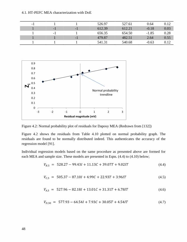
4.1. HT-PEFC MEA characterization with DoE
48
-1 1 1 526.97 527.61 0.64 0.12
1 -1 -1 612.39 612.21 -0.18 0.03
1 -1 1 656.35 654.50 -1.85 0.28
1 1 -1 479.87 482.51 2.64 0.55
1 1 1 541.31 540.68 -0.63 0.12
Figure 4.2: Normal probability plot of residuals for Daposy MEA (Redrawn from [132])
Figure 4.2 shows the residuals from Table 4.10 plotted on normal probability graph. The
residuals are found to be normally distributed indeed. This authenticates the accuracy of the
regression model [91].
Individual regression models based on the same procedure as presented above are formed for
each MEA and sample size. These models are presented in Eqns. (4.4) to (4.10) below;
𝑉𝐵,5 = 528.27 − 99.43𝐼 + 11.13𝐶 + 39.07𝑇 + 9.02𝐼𝑇 (4.4)
𝑉𝐶,5 = 505.37 − 87.10𝐼 + 4.99𝐶 + 22.93𝑇 + 3.96𝐼𝑇 (4.5)
𝑉𝐴,5 = 527.96 − 82.18𝐼 + 13.01𝐶 + 31.31𝑇 + 6.78𝐼𝑇 (4.6)
𝑉𝐷,30 = 577.93 − 64.54𝐼 + 7.93𝐶 + 30.05𝑇 + 4.54𝐼𝑇 (4.7)
0
0.1
0.2
0.3
0.4
0.5
0.6
0.7
0.8
0.9
-3 -2 -1 0 1 2 3
Z i
Residual magnitude (mV)
Normal probability trendline
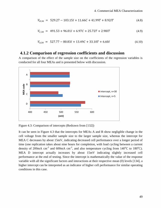
4. Commercial MEA Characterization
49
𝑉𝐵,30 = 529.27 − 103.15𝐼 + 11.66𝐶 + 41.99𝑇 + 8.92𝐼𝑇 (4.8)
𝑉𝐶,30 = 491.53 + 96.01𝐼 + 6.97𝐶 + 25.72𝑇 + 2.98𝐼𝑇 (4.9)
𝑉𝐴,30 = 527.77 − 80.83𝐼 + 13.49𝐶 + 33.10𝑇 + 6.60𝐼 (4.10)
4.1.2 Comparison of regression coefficients and discussion A comparison of the effect of the sample size on the coefficients of the regression variables is
conducted for all four MEAs and is presented below with discussion.
Figure 4.3: Comparison of intercepts (Redrawn from [132])
It can be seen in Figure 4.3 that the intercepts for MEAs A and B show negligible change in the
cell voltage from the smaller sample size to the larger sample size, whereas the intercept for
MEA C decreases by about 15mV, indicating decreased cell performance over a longer period of
time (one replication takes about nine hours for completion, with load cycling between a current
density of 200mA cm-2
and 600mA cm-2
, and also temperature cycling from 140oC to 180
oC).
MEA D intercept actually increases by about 15mV indicating slightly increased cell
performance at the end of testing. Since the intercept is mathematically the value of the response
variable with all the significant factors and interactions at their respective mean (0) levels [134], a
higher intercept can be interpreted as an indicator of higher cell performance for similar operating
conditions in this case.
400 450 500 550 600
D
C
B
A
(mV)
MEA
co
de
intercept, n=30
Intercept, n=5
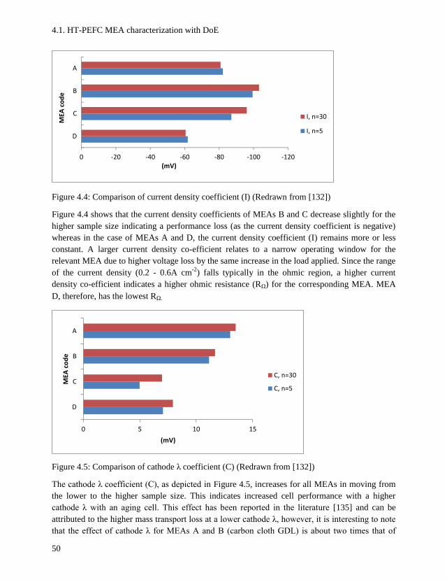
4.1. HT-PEFC MEA characterization with DoE
50
Figure 4.4: Comparison of current density coefficient (I) (Redrawn from [132])
Figure 4.4 shows that the current density coefficients of MEAs B and C decrease slightly for the
higher sample size indicating a performance loss (as the current density coefficient is negative)
whereas in the case of MEAs A and D, the current density coefficient (I) remains more or less
constant. A larger current density co-efficient relates to a narrow operating window for the
relevant MEA due to higher voltage loss by the same increase in the load applied. Since the range
of the current density (0.2 - 0.6A cm-2
) falls typically in the ohmic region, a higher current
density co-efficient indicates a higher ohmic resistance (RΩ) for the corresponding MEA. MEA
D, therefore, has the lowest RΩ.
Figure 4.5: Comparison of cathode λ coefficient (C) (Redrawn from [132])
The cathode λ coefficient (C), as depicted in Figure 4.5, increases for all MEAs in moving from
the lower to the higher sample size. This indicates increased cell performance with a higher
cathode λ with an aging cell. This effect has been reported in the literature [135] and can be
attributed to the higher mass transport loss at a lower cathode λ, however, it is interesting to note
that the effect of cathode λ for MEAs A and B (carbon cloth GDL) is about two times that of
-120-100-80-60-40-200
D
C
B
A
(mV)
MEA
co
de
I, n=30
I, n=5
0 5 10 15
D
C
B
A
(mV)
MEA
co
de
C, n=30
C, n=5
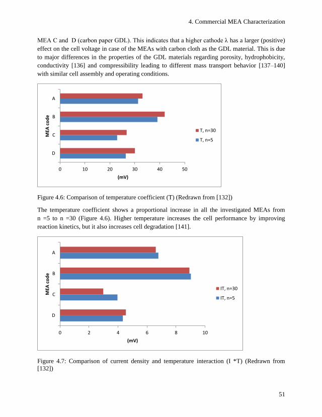
4. Commercial MEA Characterization
51
MEA C and D (carbon paper GDL). This indicates that a higher cathode λ has a larger (positive)
effect on the cell voltage in case of the MEAs with carbon cloth as the GDL material. This is due
to major differences in the properties of the GDL materials regarding porosity, hydrophobicity,
conductivity [136] and compressibility leading to different mass transport behavior [137–140]
with similar cell assembly and operating conditions.
Figure 4.6: Comparison of temperature coefficient (T) (Redrawn from [132])
The temperature coefficient shows a proportional increase in all the investigated MEAs from
n =5 to n =30 (Figure 4.6). Higher temperature increases the cell performance by improving
reaction kinetics, but it also increases cell degradation [141].
Figure 4.7: Comparison of current density and temperature interaction (I *T) (Redrawn from
[132])
0 10 20 30 40 50
D
C
B
A
(mV)
MEA
co
de
T, n=30
T, n=5
0 2 4 6 8 10
D
C
B
A
(mV)
MEA
co
de
IT, n=30
IT, n=5
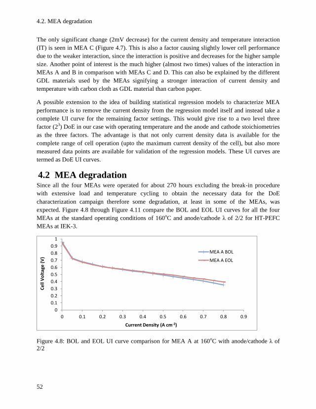
4.2. MEA degradation
52
The only significant change (2mV decrease) for the current density and temperature interaction
(IT) is seen in MEA C (Figure 4.7). This is also a factor causing slightly lower cell performance
due to the weaker interaction, since the interaction is positive and decreases for the higher sample
size. Another point of interest is the much higher (almost two times) values of the interaction in
MEAs A and B in comparison with MEAs C and D. This can also be explained by the different
GDL materials used by the MEAs signifying a stronger interaction of current density and
temperature with carbon cloth as GDL material than carbon paper.
A possible extension to the idea of building statistical regression models to characterize MEA
performance is to remove the current density from the regression model itself and instead take a
complete UI curve for the remaining factor settings. This would give rise to a two level three
factor (23) DoE in our case with operating temperature and the anode and cathode stoichiometries
as the three factors. The advantage is that not only current density data is available for the
complete range of cell operation (upto the maximum current density of the cell), but also more
measured data points are available for validation of the regression models. These UI curves are
termed as DoE UI curves.
4.2 MEA degradation Since all the four MEAs were operated for about 270 hours excluding the break-in procedure
with extensive load and temperature cycling to obtain the necessary data for the DoE
characterization campaign therefore some degradation, at least in some of the MEAs, was
expected. Figure 4.8 through Figure 4.11 compare the BOL and EOL UI curves for all the four
MEAs at the standard operating conditions of 160oC and anode/cathode λ of 2/2 for HT-PEFC
MEAs at IEK-3.
Figure 4.8: BOL and EOL UI curve comparison for MEA A at 160oC with anode/cathode λ of
2/2
0
0.1
0.2
0.3
0.4
0.5
0.6
0.7
0.8
0.9
1
0 0.1 0.2 0.3 0.4 0.5 0.6 0.7 0.8 0.9
Ce
ll V
olt
age
(V
)
Current Density (A cm-2)
MEA A BOL
MEA A EOL
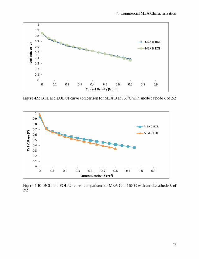
4. Commercial MEA Characterization
53
Figure 4.9: BOL and EOL UI curve comparison for MEA B at 160oC with anode/cathode λ of 2/2
Figure 4.10: BOL and EOL UI curve comparison for MEA C at 160oC with anode/cathode λ of
2/2
0
0.1
0.2
0.3
0.4
0.5
0.6
0.7
0.8
0.9
1
0 0.1 0.2 0.3 0.4 0.5 0.6 0.7 0.8 0.9
Ce
ll V
olt
age
(V
)
Current Density (A cm-2)
MEA B BOL
MEA B EOL
0
0.1
0.2
0.3
0.4
0.5
0.6
0.7
0.8
0.9
1
0 0.1 0.2 0.3 0.4 0.5 0.6 0.7 0.8 0.9
Ce
ll V
olt
age
(V
)
Current Density (A cm-2)
MEA C BOL
MEA C EOL
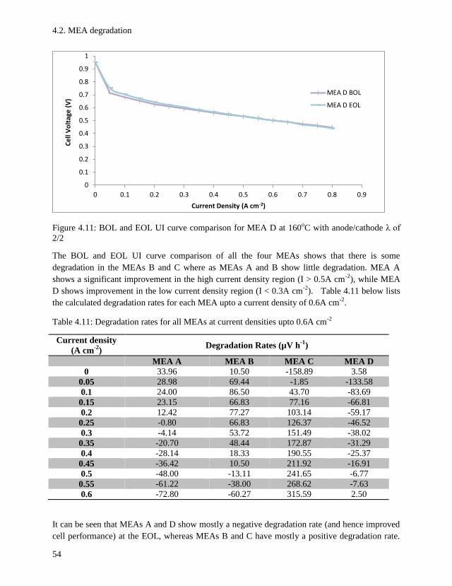
4.2. MEA degradation
54
Figure 4.11: BOL and EOL UI curve comparison for MEA D at 160oC with anode/cathode λ of
2/2
The BOL and EOL UI curve comparison of all the four MEAs shows that there is some
degradation in the MEAs B and C where as MEAs A and B show little degradation. MEA A
shows a significant improvement in the high current density region (I > 0.5A cm-2
), while MEA
D shows improvement in the low current density region (I < 0.3A cm-2
). Table 4.11 below lists
the calculated degradation rates for each MEA upto a current density of 0.6A cm-2
.
Table 4.11: Degradation rates for all MEAs at current densities upto 0.6A cm-2
Current density
(A cm-2
) Degradation Rates (µV h
-1)
MEA A MEA B MEA C MEA D
0 33.96 10.50 -158.89 3.58
0.05 28.98 69.44 -1.85 -133.58
0.1 24.00 86.50 43.70 -83.69
0.15 23.15 66.83 77.16 -66.81
0.2 12.42 77.27 103.14 -59.17
0.25 -0.80 66.83 126.37 -46.52
0.3 -4.14 53.72 151.49 -38.02
0.35 -20.70 48.44 172.87 -31.29
0.4 -28.14 18.33 190.55 -25.37
0.45 -36.42 10.50 211.92 -16.91
0.5 -48.00 -13.11 241.65 -6.77
0.55 -61.22 -38.00 268.62 -7.63
0.6 -72.80 -60.27 315.59 2.50
It can be seen that MEAs A and D show mostly a negative degradation rate (and hence improved
cell performance) at the EOL, whereas MEAs B and C have mostly a positive degradation rate.
0
0.1
0.2
0.3
0.4
0.5
0.6
0.7
0.8
0.9
1
0 0.1 0.2 0.3 0.4 0.5 0.6 0.7 0.8 0.9
Ce
ll V
olt
age
(V
)
Current Density (A cm-2)
MEA D BOL
MEA D EOL
4. Commercial MEA Characterization
55
MEA C shows the highest degradation at almost all current densities. It is deduced that MEAs A
and D are more robust for operation in fluctuating operating conditions.
4.3 Summary This chapter deals with the characterization of four commercially available HT-PEFC MEAs by
using the DoE method. The main results are listed as follows;
1. It is demonstrated that the DoE can be successfully employed to characterize MEA
performance, hence considerably reducing the experimental effort while maintaining or
improving the accuracy of results.
2. Statistical regression models are developed to predict MEA performance within a
preselected range of operating parameters. These models are based on a low sample size
(n=5) and a high sample size (n=30). A comparison of the model coefficients stipulates
that the smaller sample size (n=5) is adequate for a first evaluation of the MEA.
3. The DoE application can be further extended by utilizing the DoE UI curves for MEA
characterization.
4. Two of the MEAs (A and D) improve in performance while the other two (B and C) show
some degradation.

4.3. Summary
56

57
5 In-house Assembled MEA Study
This chapter is dedicated to finding the best material parameters for the construction of the
HT-PEFC MEA assembled at the IEK-3. The previous chapter focused on the characterization of
commercial HT-PEFC MEAs on the basis of most important operating conditions such as current
density, anode and cathode stoichiometries and the operating temperature. Besides developing
some valuable statistical models for reasonably accurate performance prediction of the MEAs,
this also helped in estimating the effects of each operating condition on the cell voltage in the
form of main effects and factor interactions of the considered operating conditions. The next step
is to evaluate the effect of material parameters on the HT-PEFC performance, which is
unfortunately not possible with the commercial MEAs. On one hand, the material parameters are
fixed and quite often confidential, for the commercial MEAs and on the other hand, no post
mortem analysis of the used MEAs is allowed due to non-disclosure agreements (NDA) with the
manufacturers.
The influence of many important material parameters on the MEA performance is nevertheless,
very significant and hence, must be investigated in a detailed manner to come up with a better
performing MEA. It is therefore decided, to use in-house assembled HT-PEFC MEAs to
investigate the most important material parameters influencing cell performance in a systematic
manner utilizing both the DoE and EIS methods.
5.1 Material parameters and MEA preparation
5.1.1 Material parameters Three of the most important material parameters (factors) for HT-PEFC operation are the Pt
loading, CCL thickness and the PADL. A brief literature review of these parameters is already
presented in section 1.1.2 and a short discussion of each factor is given in the next paragraphs.
The Pt loading is of course vital for the respective anode and cathode electrochemical reactions,
but also it is very important from a cost point of view as Pt costs can account for upto 50% of the
total cost of a fuel cell stack [72]. Different manufacturing techniques for the electrodes and the
whole MEA have been tried to improve cell performance while reducing Pt loading in HT-PEFCs
[126,142]. This will continue to be a very intense area of research until a reliable non-noble metal
catalyst can replace platinum for PEFC operation.
The CCL thickness is also of utmost importance, since the ORR taking place on the cathode side
is known to be the rate determining step with hydrogen operation [13] . The CCL thickness also
affects vitally important electrochemical parameter such as the exchange current density and the
Tafel slope [143].The CCL thickness faces contradicting requirements from a design viewpoint.
On the one hand, enough catalyst loading is needed for the required catalytic activity
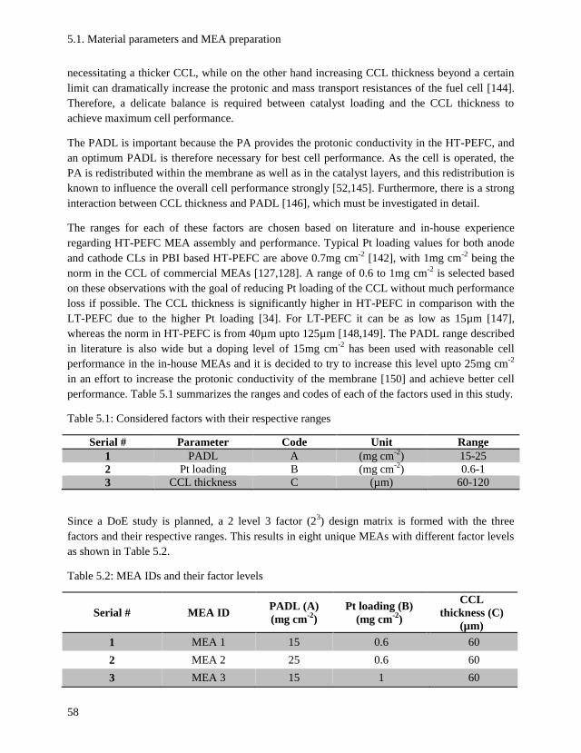
5.1. Material parameters and MEA preparation
58
necessitating a thicker CCL, while on the other hand increasing CCL thickness beyond a certain
limit can dramatically increase the protonic and mass transport resistances of the fuel cell [144].
Therefore, a delicate balance is required between catalyst loading and the CCL thickness to
achieve maximum cell performance.
The PADL is important because the PA provides the protonic conductivity in the HT-PEFC, and
an optimum PADL is therefore necessary for best cell performance. As the cell is operated, the
PA is redistributed within the membrane as well as in the catalyst layers, and this redistribution is
known to influence the overall cell performance strongly [52,145]. Furthermore, there is a strong
interaction between CCL thickness and PADL [146], which must be investigated in detail.
The ranges for each of these factors are chosen based on literature and in-house experience
regarding HT-PEFC MEA assembly and performance. Typical Pt loading values for both anode
and cathode CLs in PBI based HT-PEFC are above 0.7mg cm-2
[142], with 1mg cm-2
being the
norm in the CCL of commercial MEAs [127,128]. A range of 0.6 to 1mg cm-2
is selected based
on these observations with the goal of reducing Pt loading of the CCL without much performance
loss if possible. The CCL thickness is significantly higher in HT-PEFC in comparison with the
LT-PEFC due to the higher Pt loading [34]. For LT-PEFC it can be as low as 15µm [147],
whereas the norm in HT-PEFC is from 40µm upto 125µm [148,149]. The PADL range described
in literature is also wide but a doping level of 15mg cm-2
has been used with reasonable cell
performance in the in-house MEAs and it is decided to try to increase this level upto 25mg cm-2
in an effort to increase the protonic conductivity of the membrane [150] and achieve better cell
performance. Table 5.1 summarizes the ranges and codes of each of the factors used in this study.
Table 5.1: Considered factors with their respective ranges
Serial # Parameter Code Unit Range
1 PADL A (mg cm-2
) 15-25
2 Pt loading B (mg cm-2
) 0.6-1
3 CCL thickness C (µm) 60-120
Since a DoE study is planned, a 2 level 3 factor (23) design matrix is formed with the three
factors and their respective ranges. This results in eight unique MEAs with different factor levels
as shown in Table 5.2.
Table 5.2: MEA IDs and their factor levels
Serial # MEA ID PADL (A)
(mg cm-2
)
Pt loading (B)
(mg cm-2
)
CCL
thickness (C)
(µm)
1 MEA 1 15 0.6 60
2 MEA 2 25 0.6 60
3 MEA 3 15 1 60

5. In-house Assembled MEA Study
59
4 MEA 4 25 1 60
5 MEA 5 15 0.6 120
6 MEA 6 25 0.6 120
7 MEA 7 15 1 120
8 MEA 8 25 1 120
Each of these MEAs is also given a unique ID for easier subsequent referencing. The next step is
to prepare these MEAs.
5.1.2 MEA preparation The membranes and GDEs are prepared as described in section 3.1. The MEAs with a PADL of
25mg cm-2
use the normally doped membrane and additional 5mg cm-2
PA is added on both the
anode and cathode GDEs. Two different types of catalysts, 20 wt % and 40 wt % Pt/C, are used
for preparing the catalyst ink. To achieve different catalyst loadings and CCL thicknesses, inks
with different proportion of ingredients are used. The anode GDEs are always prepared with a Pt
loading of 0.6mg cm-2
. The absolute deviation of the Pt loading is 0.05mg cm-2
. Table 5.3
summarizes the prepared MEAs and their respective recipes for the CCL. The anode catalyst
layer recipe is always the same with 1000mg 20 wt% Pt, 3mL water, 19.5mL isopropanol and
744µL PTFE. This leads to a Pt loading of 0.6mg cm-2
and a CL thickness of 60µm for all the
anodes.
Table 5.3: Cathode catalyst layer recipes and spacer thicknesses used for GDE preparation
(Reprinted with permission from [151], Copyright [2017], The Electrochemical Society.)
MEA ID Recipe for the CCL Thickness of spacer
(mm)
MEA 1
1000mg 20 wt.% Pt/C, 3.0mL
water, 19.5mL isopropanol,
744µL PTFE
0.5
MEA 2
1000mg 20 wt.% Pt/C, 3.0mL
water, 19.5mL isopropanol,
744µL PTFE
0.5
MEA 3
500mg 40 wt.% Pt/C, 1.178mL
water, 7.66mL isopropanol,
225µL PTFE
0.4
MEA 4
500mg 40 wt.% Pt/C, 1.178mL
water, 7.66mL isopropanol,
225µL PTFE
0.4
MEA 5 16 wt.% Pt/C (800mg 20 wt.% 0.8
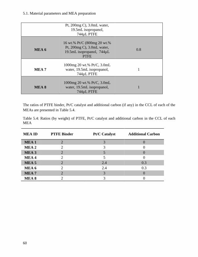
5.1. Material parameters and MEA preparation
60
Pt, 200mg C), 3.0mL water,
19.5mL isopropanol,
744µL PTFE
MEA 6
16 wt.% Pt/C (800mg 20 wt.%
Pt, 200mg C), 3.0mL water,
19.5mL isopropanol, 744µL
PTFE
0.8
MEA 7
1000mg 20 wt.% Pt/C, 3.0mL
water, 19.5mL isopropanol,
744µL PTFE
1
MEA 8
1000mg 20 wt.% Pt/C, 3.0mL
water, 19.5mL isopropanol,
744µL PTFE
1
The ratios of PTFE binder, Pt/C catalyst and additional carbon (if any) in the CCL of each of the
MEAs are presented in Table 5.4.
Table 5.4: Ratios (by weight) of PTFE, Pt/C catalyst and additional carbon in the CCL of each
MEA
MEA ID PTFE Binder Pt/C Catalyst Additional Carbon
MEA 1 2 3 0
MEA 2 2 3 0
MEA 3 2 5 0
MEA 4 2 5 0
MEA 5 2 2.4 0.3
MEA 6 2 2.4 0.3
MEA 7 2 3 0
MEA 8 2 3 0
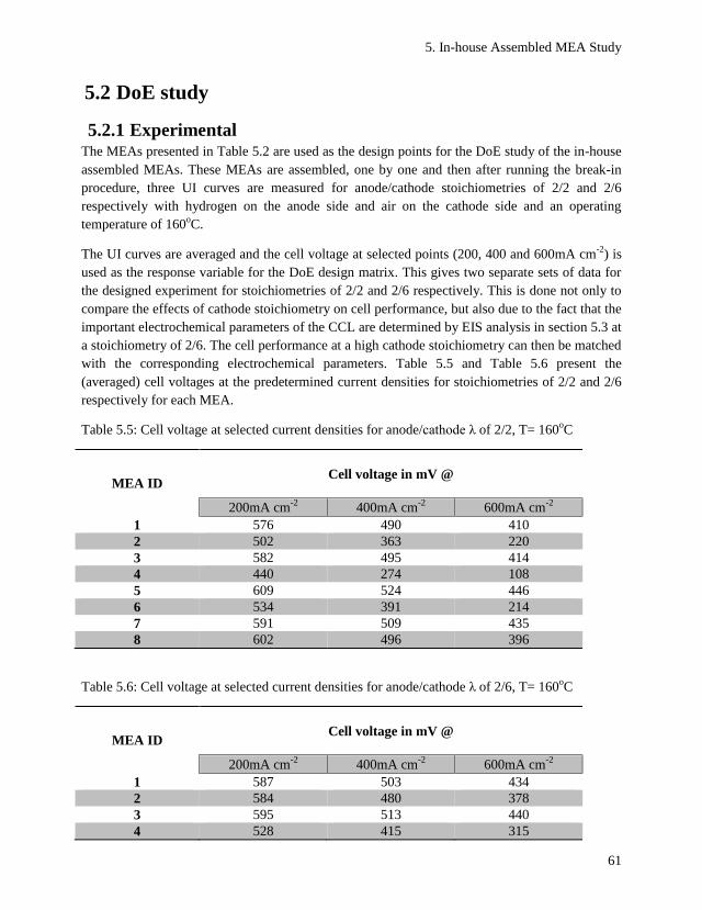
5. In-house Assembled MEA Study
61
5.2 DoE study
5.2.1 Experimental The MEAs presented in Table 5.2 are used as the design points for the DoE study of the in-house
assembled MEAs. These MEAs are assembled, one by one and then after running the break-in
procedure, three UI curves are measured for anode/cathode stoichiometries of 2/2 and 2/6
respectively with hydrogen on the anode side and air on the cathode side and an operating
temperature of 160oC.
The UI curves are averaged and the cell voltage at selected points (200, 400 and 600mA cm-2
) is
used as the response variable for the DoE design matrix. This gives two separate sets of data for
the designed experiment for stoichiometries of 2/2 and 2/6 respectively. This is done not only to
compare the effects of cathode stoichiometry on cell performance, but also due to the fact that the
important electrochemical parameters of the CCL are determined by EIS analysis in section 5.3 at
a stoichiometry of 2/6. The cell performance at a high cathode stoichiometry can then be matched
with the corresponding electrochemical parameters. Table 5.5 and Table 5.6 present the
(averaged) cell voltages at the predetermined current densities for stoichiometries of 2/2 and 2/6
respectively for each MEA.
Table 5.5: Cell voltage at selected current densities for anode/cathode λ of 2/2, T= 160oC
MEA ID
Cell voltage in mV @
200mA cm-2
400mA cm-2
600mA cm-2
1 576 490 410
2 502 363 220
3 582 495 414
4 440 274 108
5 609 524 446
6 534 391 214
7 591 509 435
8 602 496 396
Table 5.6: Cell voltage at selected current densities for anode/cathode λ of 2/6, T= 160oC
MEA ID
Cell voltage in mV @
200mA cm-2
400mA cm-2
600mA cm-2
1 587 503 434
2 584 480 378
3 595 513 440
4 528 415 315
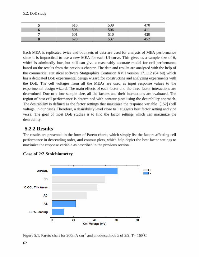
5.2. DoE study
62
5 616 539 470
6 598 506 411
7 601 510 430
8 628 537 452
Each MEA is replicated twice and both sets of data are used for analysis of MEA performance
since it is impractical to use a new MEA for each UI curve. This gives us a sample size of 6,
which is admittedly low, but still can give a reasonably accurate model for cell performance
based on the results from the previous chapter. The data and results are analyzed with the help of
the commercial statistical software Statgraphics Centurion XVII version 17.1.12 (64 bit) which
has a dedicated DoE experimental design wizard for constructing and analyzing experiments with
the DoE. The cell voltages from all the MEAs are used as input response values to the
experimental design wizard. The main effects of each factor and the three factor interactions are
determined. Due to a low sample size, all the factors and their interactions are evaluated. The
region of best cell performance is determined with contour plots using the desirability approach.
The desirability is defined as the factor settings that maximize the response variable [152] (cell
voltage, in our case). Therefore, a desirability level close to 1 suggests best factor setting and vice
versa. The goal of most DoE studies is to find the factor settings which can maximize the
desirability.
5.2.2 Results The results are presented in the form of Pareto charts, which simply list the factors affecting cell
performance in descending order, and contour plots, which help depict the best factor settings to
maximize the response variable as described in the previous section.
Case of 2/2 Stoichiometry
Figure 5.1: Pareto chart for 200mA cm-2
and anode/cathode λ of 2/2, T= 160oC
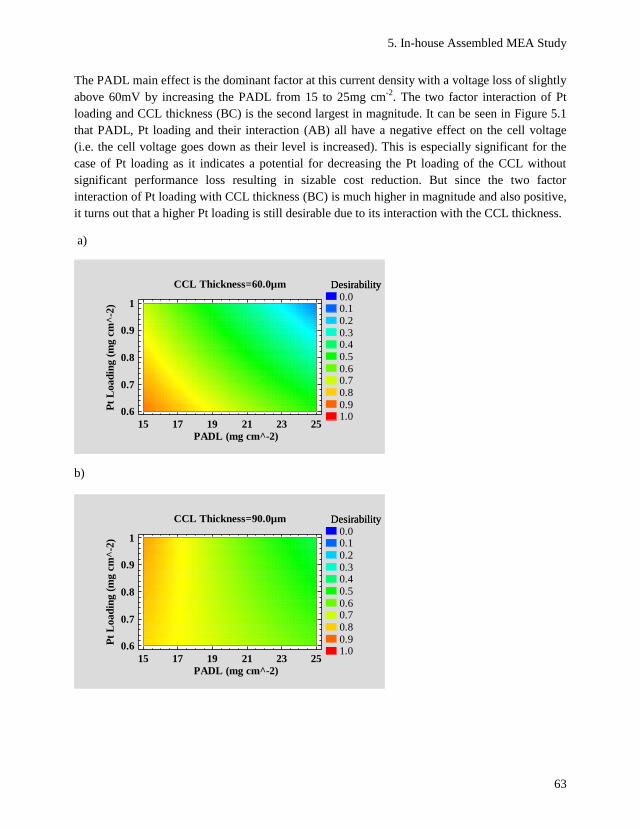
5. In-house Assembled MEA Study
63
The PADL main effect is the dominant factor at this current density with a voltage loss of slightly
above 60mV by increasing the PADL from 15 to 25mg cm-2
. The two factor interaction of Pt
loading and CCL thickness (BC) is the second largest in magnitude. It can be seen in Figure 5.1
that PADL, Pt loading and their interaction (AB) all have a negative effect on the cell voltage
(i.e. the cell voltage goes down as their level is increased). This is especially significant for the
case of Pt loading as it indicates a potential for decreasing the Pt loading of the CCL without
significant performance loss resulting in sizable cost reduction. But since the two factor
interaction of Pt loading with CCL thickness (BC) is much higher in magnitude and also positive,
it turns out that a higher Pt loading is still desirable due to its interaction with the CCL thickness.
a)
b)
CCL Thickness=60.0µm
PADL (mg cm^-2)
Pt
Load
ing (
mg c
m^
-2)
15 17 19 21 23 25
0.6
0.7
0.8
0.9
1
Desirability0.00.10.20.30.40.50.60.70.80.91.0
Desirability
CCL Thickness=90.0µm
PADL (mg cm^-2)
Pt
Load
ing (
mg c
m^
-2)
15 17 19 21 23 25
0.6
0.7
0.8
0.9
1
Desirability0.00.10.20.30.40.50.60.70.80.91.0
Desirability
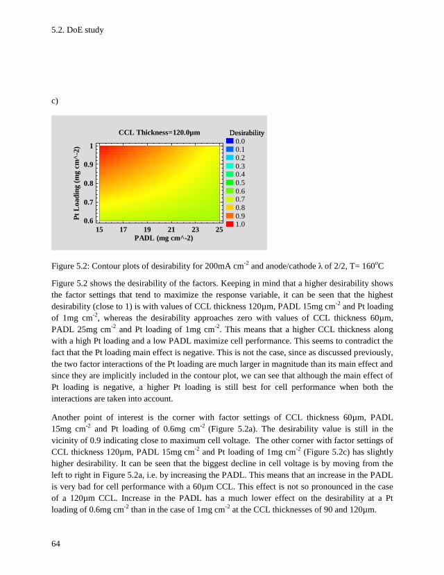
5.2. DoE study
64
c)
Figure 5.2: Contour plots of desirability for 200mA cm-2
and anode/cathode λ of 2/2, T= 160oC
Figure 5.2 shows the desirability of the factors. Keeping in mind that a higher desirability shows
the factor settings that tend to maximize the response variable, it can be seen that the highest
desirability (close to 1) is with values of CCL thickness 120µm, PADL 15mg cm-2
and Pt loading
of 1mg cm-2
, whereas the desirability approaches zero with values of CCL thickness 60µm,
PADL 25mg cm-2
and Pt loading of 1mg cm-2
. This means that a higher CCL thickness along
with a high Pt loading and a low PADL maximize cell performance. This seems to contradict the
fact that the Pt loading main effect is negative. This is not the case, since as discussed previously,
the two factor interactions of the Pt loading are much larger in magnitude than its main effect and
since they are implicitly included in the contour plot, we can see that although the main effect of
Pt loading is negative, a higher Pt loading is still best for cell performance when both the
interactions are taken into account.
Another point of interest is the corner with factor settings of CCL thickness 60µm, PADL
15mg cm-2
and Pt loading of 0.6mg cm-2
(Figure 5.2a). The desirability value is still in the
vicinity of 0.9 indicating close to maximum cell voltage. The other corner with factor settings of
CCL thickness 120µm, PADL 15mg cm-2
and Pt loading of 1mg cm-2
(Figure 5.2c) has slightly
higher desirability. It can be seen that the biggest decline in cell voltage is by moving from the
left to right in Figure 5.2a, i.e. by increasing the PADL. This means that an increase in the PADL
is very bad for cell performance with a 60µm CCL. This effect is not so pronounced in the case
of a 120µm CCL. Increase in the PADL has a much lower effect on the desirability at a Pt
loading of 0.6mg cm-2
than in the case of 1mg cm-2
at the CCL thicknesses of 90 and 120µm.
CCL Thickness=120.0µm
PADL (mg cm^-2)
Pt
Load
ing (
mg c
m^
-2)
15 17 19 21 23 25
0.6
0.7
0.8
0.9
1
Desirability0.00.10.20.30.40.50.60.70.80.91.0
Desirability
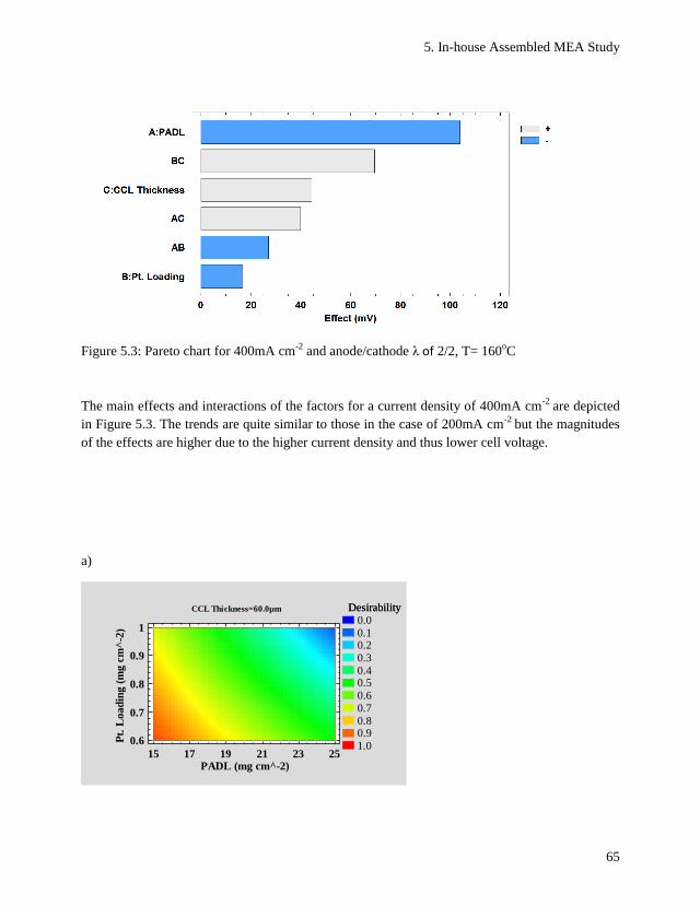
5. In-house Assembled MEA Study
65
Figure 5.3: Pareto chart for 400mA cm-2
and anode/cathode λ of 2/2, T= 160oC
The main effects and interactions of the factors for a current density of 400mA cm-2
are depicted
in Figure 5.3. The trends are quite similar to those in the case of 200mA cm-2
but the magnitudes
of the effects are higher due to the higher current density and thus lower cell voltage.
a)
CCL Thickness=60.0µm
PADL (mg cm^-2)
Pt.
Lo
ad
ing
(m
g c
m^
-2)
0.40.50.60.70.8
15 17 19 21 23 25
0.6
0.7
0.8
0.9
1
Desirability0.00.10.20.30.40.50.60.70.80.91.0
Desirability
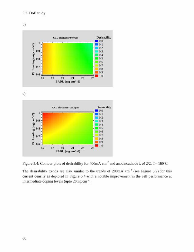
5.2. DoE study
66
b)
c)
Figure 5.4: Contour plots of desirability for 400mA cm-2
and anode/cathode λ of 2/2, T= 160oC
The desirability trends are also similar to the trends of 200mA cm-2
(see Figure 5.2) for this
current density as depicted in Figure 5.4 with a notable improvement in the cell performance at
intermediate doping levels (upto 20mg cm-2
).
CCL Thickness=90.0µm
PADL (mg cm^-2)
Pt.
Lo
ad
ing
(m
g c
m^
-2)
0.40.50.60.70.8
15 17 19 21 23 25
0.6
0.7
0.8
0.9
1
Desirability0.00.10.20.30.40.50.60.70.80.91.0
Desirability
CCL Thickness=120.0µm
PADL (mg cm^-2)
Pt.
Lo
ad
ing
(m
g c
m^
-2)
0.40.50.60.70.8
15 17 19 21 23 25
0.6
0.7
0.8
0.9
1
Desirability0.00.10.20.30.40.50.60.70.80.91.0
Desirability
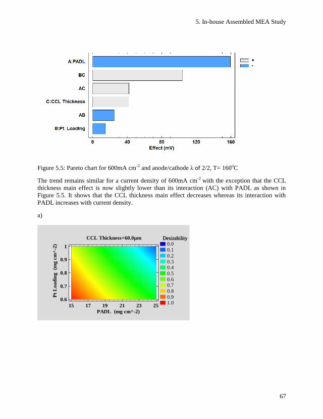
5. In-house Assembled MEA Study
67
Figure 5.5: Pareto chart for 600mA cm-2
and anode/cathode λ of 2/2, T= 160oC
The trend remains similar for a current density of 600mA cm-2
with the exception that the CCL
thickness main effect is now slightly lower than its interaction (AC) with PADL as shown in
Figure 5.5. It shows that the CCL thickness main effect decreases whereas its interaction with
PADL increases with current density.
a)
PADL (mg cm^-2)
Pt
Lo
ad
ing
(m
g c
m^
-2)
CCL Thickness=60.0µm
15 17 19 21 23 25
0.6
0.7
0.8
0.9
1
Desirability0.00.10.20.30.40.50.60.70.80.91.0
Desirability
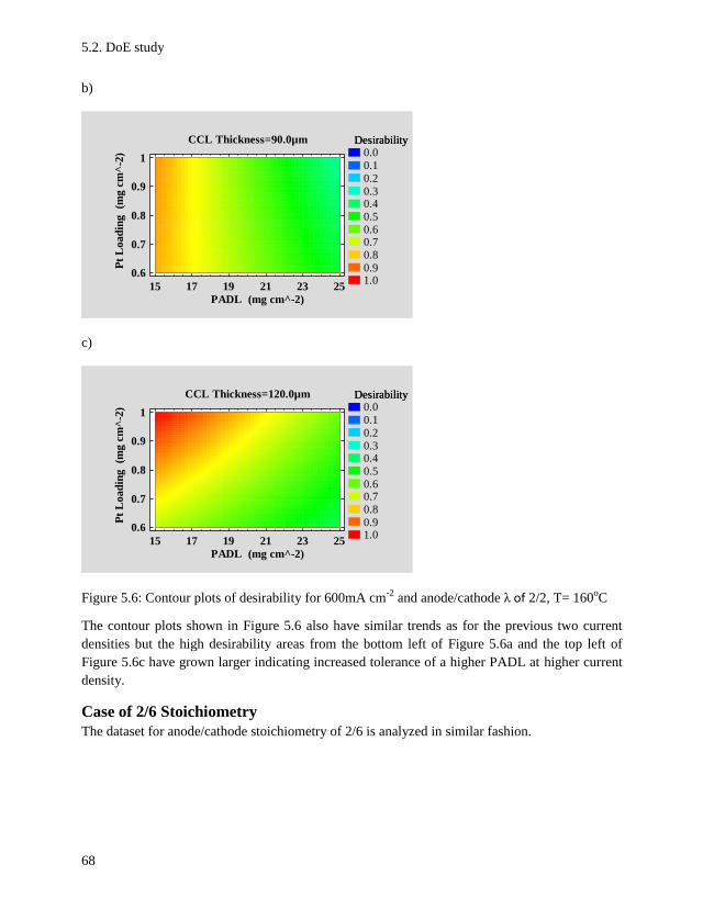
5.2. DoE study
68
b)
c)
Figure 5.6: Contour plots of desirability for 600mA cm-2
and anode/cathode λ of 2/2, T= 160oC
The contour plots shown in Figure 5.6 also have similar trends as for the previous two current
densities but the high desirability areas from the bottom left of Figure 5.6a and the top left of
Figure 5.6c have grown larger indicating increased tolerance of a higher PADL at higher current
density.
Case of 2/6 Stoichiometry
The dataset for anode/cathode stoichiometry of 2/6 is analyzed in similar fashion.
PADL (mg cm^-2)
Pt
Lo
ad
ing
(m
g c
m^
-2)
CCL Thickness=90.0µm
15 17 19 21 23 25
0.6
0.7
0.8
0.9
1
Desirability0.00.10.20.30.40.50.60.70.80.91.0
Desirability
PADL (mg cm^-2)
Pt
Lo
ad
ing
(m
g c
m^
-2)
CCL Thickness=120.0µm
15 17 19 21 23 25
0.6
0.7
0.8
0.9
1
Desirability0.00.10.20.30.40.50.60.70.80.91.0
Desirability
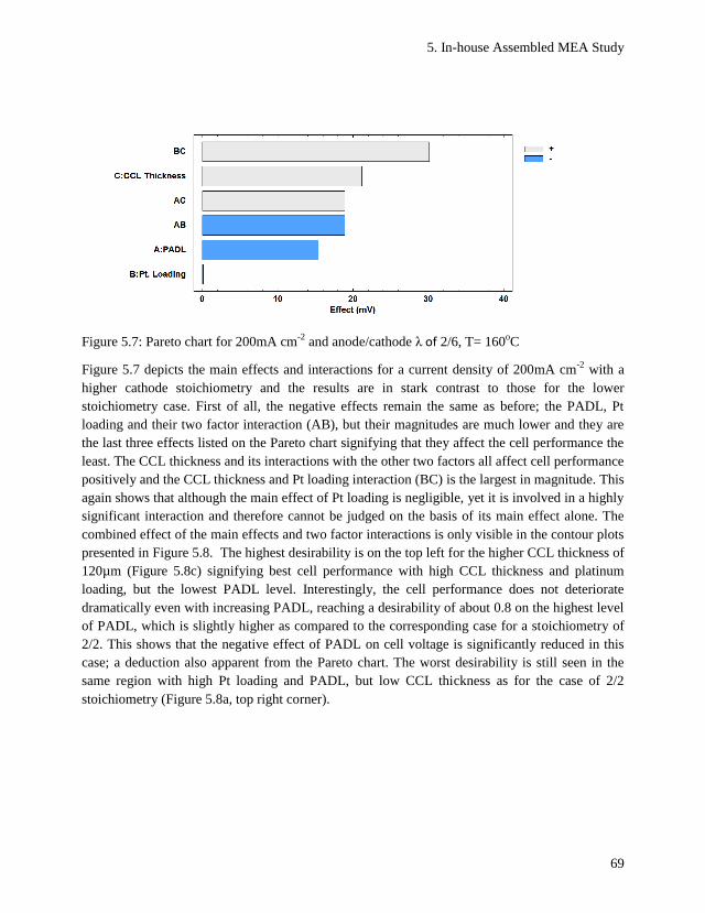
5. In-house Assembled MEA Study
69
Figure 5.7: Pareto chart for 200mA cm-2
and anode/cathode λ of 2/6, T= 160oC
Figure 5.7 depicts the main effects and interactions for a current density of 200mA cm-2
with a
higher cathode stoichiometry and the results are in stark contrast to those for the lower
stoichiometry case. First of all, the negative effects remain the same as before; the PADL, Pt
loading and their two factor interaction (AB), but their magnitudes are much lower and they are
the last three effects listed on the Pareto chart signifying that they affect the cell performance the
least. The CCL thickness and its interactions with the other two factors all affect cell performance
positively and the CCL thickness and Pt loading interaction (BC) is the largest in magnitude. This
again shows that although the main effect of Pt loading is negligible, yet it is involved in a highly
significant interaction and therefore cannot be judged on the basis of its main effect alone. The
combined effect of the main effects and two factor interactions is only visible in the contour plots
presented in Figure 5.8. The highest desirability is on the top left for the higher CCL thickness of
120µm (Figure 5.8c) signifying best cell performance with high CCL thickness and platinum
loading, but the lowest PADL level. Interestingly, the cell performance does not deteriorate
dramatically even with increasing PADL, reaching a desirability of about 0.8 on the highest level
of PADL, which is slightly higher as compared to the corresponding case for a stoichiometry of
2/2. This shows that the negative effect of PADL on cell voltage is significantly reduced in this
case; a deduction also apparent from the Pareto chart. The worst desirability is still seen in the
same region with high Pt loading and PADL, but low CCL thickness as for the case of 2/2
stoichiometry (Figure 5.8a, top right corner).
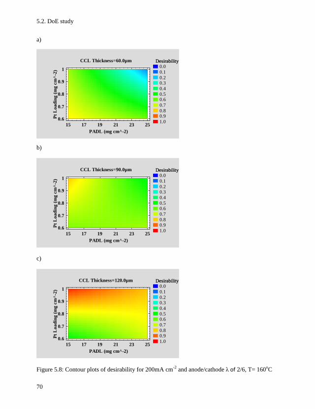
5.2. DoE study
70
a)
b)
c)
Figure 5.8: Contour plots of desirability for 200mA cm-2
and anode/cathode λ of 2/6, T= 160oC
CCL Thickness=60.0µm
PADL (mg cm^-2)
Pt
Lo
ad
ing
(m
g c
m^
-2)
15 17 19 21 23 25
0.6
0.7
0.8
0.9
1
Desirability0.00.10.20.30.40.50.60.70.80.91.0
Desirability
CCL Thickness=90.0µm
PADL (mg cm^-2)
Pt
Lo
ad
ing
(m
g c
m^
-2)
15 17 19 21 23 25
0.6
0.7
0.8
0.9
1
Desirability0.00.10.20.30.40.50.60.70.80.91.0
Desirability
CCL Thickness=120.0µm
PADL (mg cm^-2)
Pt
Lo
ad
ing
(m
g c
m^
-2)
15 17 19 21 23 25
0.6
0.7
0.8
0.9
1
Desirability0.00.10.20.30.40.50.60.70.80.91.0
Desirability
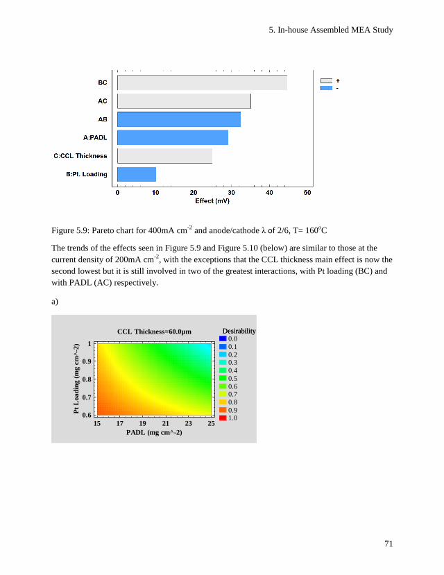
5. In-house Assembled MEA Study
71
Figure 5.9: Pareto chart for 400mA cm-2
and anode/cathode λ of 2/6, T= 160oC
The trends of the effects seen in Figure 5.9 and Figure 5.10 (below) are similar to those at the
current density of 200mA cm-2
, with the exceptions that the CCL thickness main effect is now the
second lowest but it is still involved in two of the greatest interactions, with Pt loading (BC) and
with PADL (AC) respectively.
a)
CCL Thickness=60.0µm
PADL (mg cm^-2)
Pt
Load
ing (
mg c
m^
-2)
15 17 19 21 23 25
0.6
0.7
0.8
0.9
1
Desirability0.00.10.20.30.40.50.60.70.80.91.0
Desirability
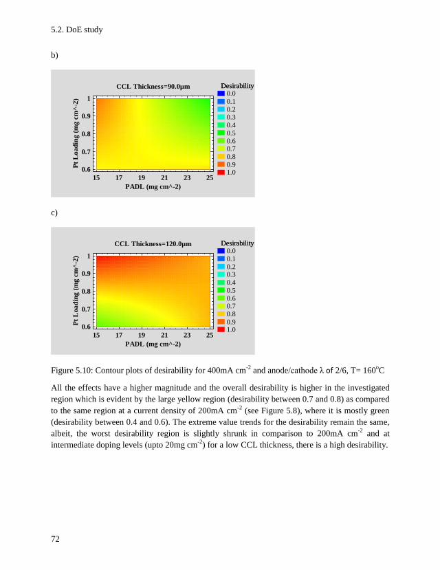
5.2. DoE study
72
b)
c)
Figure 5.10: Contour plots of desirability for 400mA cm-2
and anode/cathode λ of 2/6, T= 160oC
All the effects have a higher magnitude and the overall desirability is higher in the investigated
region which is evident by the large yellow region (desirability between 0.7 and 0.8) as compared
to the same region at a current density of 200mA cm-2
(see Figure 5.8), where it is mostly green
(desirability between 0.4 and 0.6). The extreme value trends for the desirability remain the same,
albeit, the worst desirability region is slightly shrunk in comparison to 200mA cm-2
and at
intermediate doping levels (upto 20mg cm-2
) for a low CCL thickness, there is a high desirability.
CCL Thickness=90.0µm
PADL (mg cm^-2)
Pt
Lo
ad
ing
(m
g c
m^
-2)
15 17 19 21 23 25
0.6
0.7
0.8
0.9
1
Desirability0.00.10.20.30.40.50.60.70.80.91.0
Desirability
CCL Thickness=120.0µm
PADL (mg cm^-2)
Pt
Lo
ad
ing
(m
g c
m^
-2)
15 17 19 21 23 25
0.6
0.7
0.8
0.9
1
Desirability0.00.10.20.30.40.50.60.70.80.91.0
Desirability
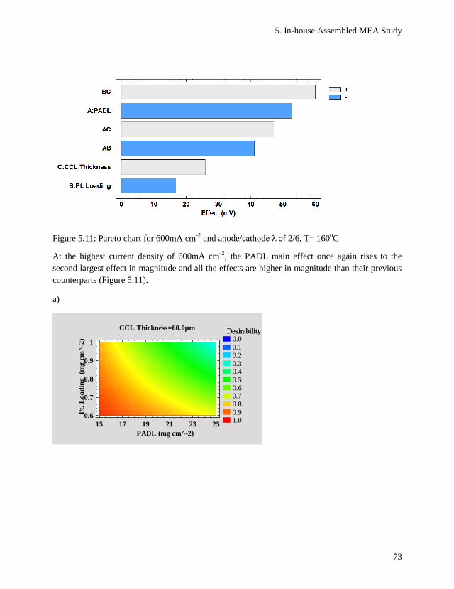
5. In-house Assembled MEA Study
73
Figure 5.11: Pareto chart for 600mA cm-2
and anode/cathode λ of 2/6, T= 160oC
At the highest current density of 600mA cm-2
, the PADL main effect once again rises to the
second largest effect in magnitude and all the effects are higher in magnitude than their previous
counterparts (Figure 5.11).
a)
CCL Thickness=60.0µm
PADL (mg cm^-2)
Pt.
Load
ing
(mg c
m^
-2)
15 17 19 21 23 25
0.6
0.7
0.8
0.9
1
Desirability0.00.10.20.30.40.50.60.70.80.91.0
Desirability
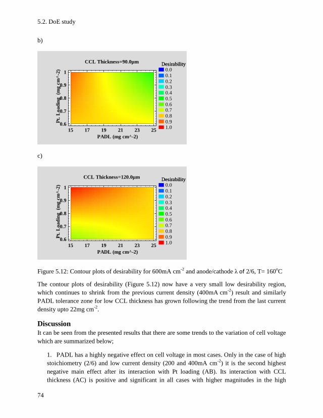
5.2. DoE study
74
b)
c)
Figure 5.12: Contour plots of desirability for 600mA cm-2
and anode/cathode λ of 2/6, T= 160oC
The contour plots of desirability (Figure 5.12) now have a very small low desirability region,
which continues to shrink from the previous current density (400mA cm-2
) result and similarly
PADL tolerance zone for low CCL thickness has grown following the trend from the last current
density upto 22mg cm-2
.
Discussion
It can be seen from the presented results that there are some trends to the variation of cell voltage
which are summarized below;
1. PADL has a highly negative effect on cell voltage in most cases. Only in the case of high
stoichiometry (2/6) and low current density (200 and 400mA cm-2
) it is the second highest
negative main effect after its interaction with Pt loading (AB). Its interaction with CCL
thickness (AC) is positive and significant in all cases with higher magnitudes in the high
CCL Thickness=90.0µm
PADL (mg cm^-2)
Pt.
Load
ing
(mg c
m^
-2)
15 17 19 21 23 25
0.6
0.7
0.8
0.9
1
Desirability0.00.10.20.30.40.50.60.70.80.91.0
Desirability
CCL Thickness=120.0µm
PADL (mg cm^-2)
Pt.
Load
ing
(mg c
m^
-2)
15 17 19 21 23 25
0.6
0.7
0.8
0.9
1
Desirability0.00.10.20.30.40.50.60.70.80.91.0
Desirability
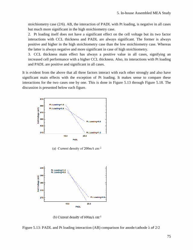
5. In-house Assembled MEA Study
75
stoichiometry case (2/6). AB, the interaction of PADL with Pt loading, is negative in all cases
but much more significant in the high stoichiometry case.
2. Pt loading itself does not have a significant effect on the cell voltage but its two factor
interactions with CCL thickness and PADL are always significant. The former is always
positive and higher in the high stoichiometry case than the low stoichiometry case. Whereas
the latter is always negative and more significant in case of high stoichiometry.
3. CCL thickness main effect has always a positive value in all cases, signifying an
increased cell performance with a higher CCL thickness. Also, its interactions with Pt loading
and PADL are positive and significant in all cases.
It is evident from the above that all three factors interact with each other strongly and also have
significant main effects with the exception of Pt loading. It makes sense to compare these
interactions for the two cases one by one. This is done in Figure 5.13 through Figure 5.18. The
discussion is presented below each figure.
Figure 5.13: PADL and Pt loading interaction (AB) comparison for anode/cathode λ of 2/2
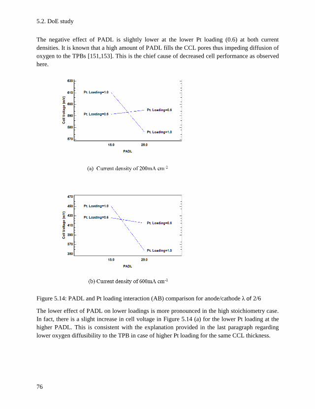
5.2. DoE study
76
The negative effect of PADL is slightly lower at the lower Pt loading (0.6) at both current
densities. It is known that a high amount of PADL fills the CCL pores thus impeding diffusion of
oxygen to the TPBs [151,153]. This is the chief cause of decreased cell performance as observed
here.
Figure 5.14: PADL and Pt loading interaction (AB) comparison for anode/cathode λ of 2/6
The lower effect of PADL on lower loadings is more pronounced in the high stoichiometry case.
In fact, there is a slight increase in cell voltage in Figure 5.14 (a) for the lower Pt loading at the
higher PADL. This is consistent with the explanation provided in the last paragraph regarding
lower oxygen diffusibility to the TPB in case of higher Pt loading for the same CCL thickness.
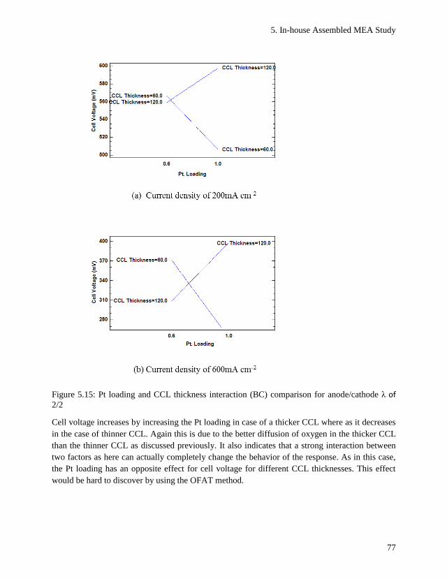
5. In-house Assembled MEA Study
77
Figure 5.15: Pt loading and CCL thickness interaction (BC) comparison for anode/cathode λ of 2/2
Cell voltage increases by increasing the Pt loading in case of a thicker CCL where as it decreases
in the case of thinner CCL. Again this is due to the better diffusion of oxygen in the thicker CCL
than the thinner CCL as discussed previously. It also indicates that a strong interaction between
two factors as here can actually completely change the behavior of the response. As in this case,
the Pt loading has an opposite effect for cell voltage for different CCL thicknesses. This effect
would be hard to discover by using the OFAT method.
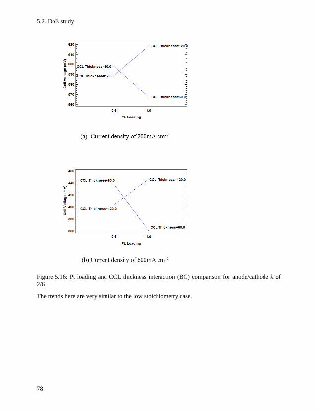
5.2. DoE study
78
Figure 5.16: Pt loading and CCL thickness interaction (BC) comparison for anode/cathode λ of 2/6
The trends here are very similar to the low stoichiometry case.
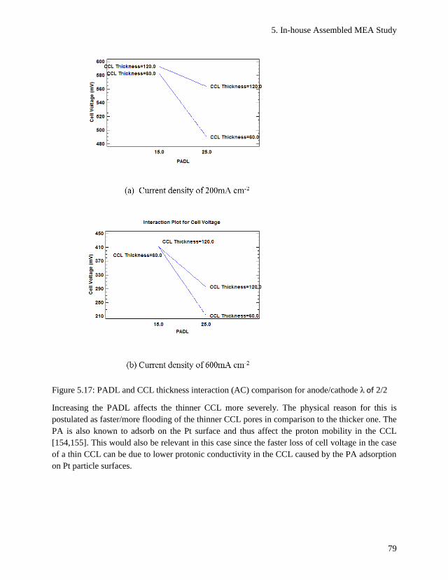
5. In-house Assembled MEA Study
79
Figure 5.17: PADL and CCL thickness interaction (AC) comparison for anode/cathode λ of 2/2
Increasing the PADL affects the thinner CCL more severely. The physical reason for this is
postulated as faster/more flooding of the thinner CCL pores in comparison to the thicker one. The
PA is also known to adsorb on the Pt surface and thus affect the proton mobility in the CCL
[154,155]. This would also be relevant in this case since the faster loss of cell voltage in the case
of a thin CCL can be due to lower protonic conductivity in the CCL caused by the PA adsorption
on Pt particle surfaces.
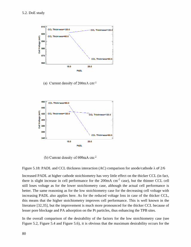
5.2. DoE study
80
Figure 5.18: PADL and CCL thickness interaction (AC) comparison for anode/cathode λ of 2/6
Increased PADL at higher cathode stoichiometry has very little effect on the thicker CCL (in fact,
there is slight increase in cell performance for the 200mA cm-2
case), but the thinner CCL cell
still loses voltage as for the lower stoichiometry case, although the actual cell performance is
better. The same reasoning as for the low stoichiometry case for the decreasing cell voltage with
increasing PADL also applies here. As for the reduced voltage loss in case of the thicker CCL,
this means that the higher stoichiometry improves cell performance. This is well known in the
literature [32,35], but the improvement is much more pronounced for the thicker CCL because of
lesser pore blockage and PA adsorption on the Pt particles, thus enhancing the TPB sites.
In the overall comparison of the desirability of the factors for the low stoichiometry case (see
Figure 5.2, Figure 5.4 and Figure 5.6), it is obvious that the maximum desirability occurs for the
5. In-house Assembled MEA Study
81
thicker CCL (120µm) with a PADL of 15mg cm-2
and a Pt loading of 1mg cm-2
for both current
densities. Also, the PADL tolerance of the thicker CCL is much higher than its thinner
counterpart. There is decrease in desirability by increasing the Pt loading for the thinner CCL and
vice versa.
The desirability follows a similar pattern for the higher stoichiometry case (see Figure 5.8, Figure
5.10 and Figure 5.12) as for the lower stoichiometry case. There is still strong negative PADL
effect for the thinner CCL, whereas the thicker CCL is more or less stable in this regard. The loss
in desirability by increasing the Pt loading for the thinner CCL is much less pronounced but the
increase in the thicker CCL is much more pronounced for a lower PADL while stable at the
higher PADL. Since a higher PADL improves the protonic conductivity of the membrane and the
CCL [156], the method of doping the membrane and the doping time can be improved to get
better performing MEAs [52] as many high performing HT-PEFC MEAs have a high phosphoric
acid content with specialized doping methods such as the sol-gel method of the Celtec®
PW1100
BASF MEA.
The highest desirability is achieved for the factor settings of low PADL (15mg cm-2
), high CCL
thickness (120µm) and high Pt loading (1mg cm-2
) for most cases. The corresponding MEA with
these settings is MEA 7, which is therefore selected as the MEA with the most desirable factor
settings, but still with further room for improvement, especially with regard to PA doping due to
its high influence on cell performance.
5.3 EIS study The EIS study is done as a supplement to the DoE study to verify the findings and also
investigate the important electrochemical parameters of the cell to have a clearer picture of the
dominant parameters affecting cell performance. This will help to pinpoint improvement areas
and determine the methodology to implement those improvements to have better performing PBI
based HT-PEFC MEAs in future.
5.3.1 Experimental All the MEAs are subjected to EIS measurements immediately after the break-in procedure is
finished and the UI curves have been taken. The aim is to characterize the CCL and determine its
most important electrochemical parameters. This can be achieved by measuring the cell
impedance at very low current densities (typically upto 100mA cm-2
) and a high cathode
stoichiometry (minimum 10) to ensure very high and constant oxygen concentration throughout
the catalyst layer. This ensures almost no contribution to the mass transport losses from the lack
of oxygen diffusion to the TPB at the membrane/CCL interface and instead all the resistance
shown by the cell in the low frequency region of the Nyquist plot can be attributed exclusively to
the CCL itself [123,151,157] . The relevant electrochemical parameters of the CCL can therefore
be extracted by fitting a simple ECM to the impedance data [158,159].
Four current densities are selected for impedance measurements, 10, 20, 50 and 100mA cm-2
respectively. The aim is to observe the variation in the electrochemical parameters of the cell
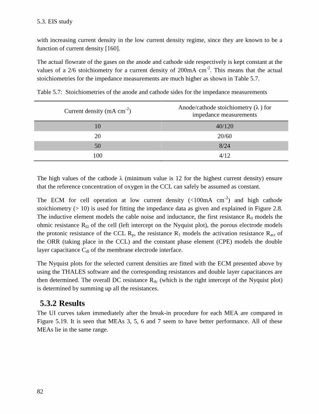
5.3. EIS study
82
with increasing current density in the low current density regime, since they are known to be a
function of current density [160].
The actual flowrate of the gases on the anode and cathode side respectively is kept constant at the
values of a 2/6 stoichiometry for a current density of 200mA cm-2
. This means that the actual
stoichiometries for the impedance measurements are much higher as shown in Table 5.7.
Table 5.7: Stoichiometries of the anode and cathode sides for the impedance measurements
Current density (mA cm-2
) Anode/cathode stoichiometry (λ ) for
impedance measurements
10 40/120
20 20/60
50 8/24
100 4/12
The high values of the cathode λ (minimum value is 12 for the highest current density) ensure
that the reference concentration of oxygen in the CCL can safely be assumed as constant.
The ECM for cell operation at low current density (<100mA cm-2
) and high cathode
stoichiometry (> 10) is used for fitting the impedance data as given and explained in Figure 2.8.
The inductive element models the cable noise and inductance, the first resistance R0 models the
ohmic resistance RΩ of the cell (left intercept on the Nyquist plot), the porous electrode models
the protonic resistance of the CCL Rp, the resistance R1 models the activation resistance Ract of
the ORR (taking place in the CCL) and the constant phase element (CPE) models the double
layer capacitance Cdl of the membrane electrode interface.
The Nyquist plots for the selected current densities are fitted with the ECM presented above by
using the THALES software and the corresponding resistances and double layer capacitances are
then determined. The overall DC resistance Rdc (which is the right intercept of the Nyquist plot)
is determined by summing up all the resistances.
5.3.2 Results The UI curves taken immediately after the break-in procedure for each MEA are compared in
Figure 5.19. It is seen that MEAs 3, 5, 6 and 7 seem to have better performance. All of these
MEAs lie in the same range.
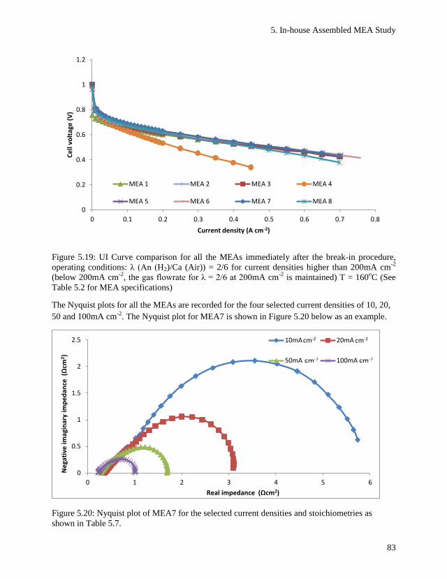
5. In-house Assembled MEA Study
83
Figure 5.19: UI Curve comparison for all the MEAs immediately after the break-in procedure,
operating conditions: λ (An (H2)/Ca (Air)) = 2/6 for current densities higher than 200mA cm-2
(below 200mA cm-2
, the gas flowrate for λ = 2/6 at 200mA cm-2
is maintained) T = 160oC (See
Table 5.2 for MEA specifications)
The Nyquist plots for all the MEAs are recorded for the four selected current densities of 10, 20,
50 and 100mA cm-2
. The Nyquist plot for MEA7 is shown in Figure 5.20 below as an example.
Figure 5.20: Nyquist plot of MEA7 for the selected current densities and stoichiometries as
shown in Table 5.7.
0
0.2
0.4
0.6
0.8
1
1.2
0 0.1 0.2 0.3 0.4 0.5 0.6 0.7 0.8
Ce
ll vo
ltag
e (
V)
Current density (A cm-2)
MEA 1 MEA 2 MEA 3 MEA 4
MEA 5 MEA 6 MEA 7 MEA 8
0
0.5
1
1.5
2
2.5
0 1 2 3 4 5 6
Ne
gati
ve im
agin
ary
imp
ed
ance
(Ω
cm2 )
Real impedance (Ωcm2)
10mA 20mA
50mA 100mA
cm-2 cm-2
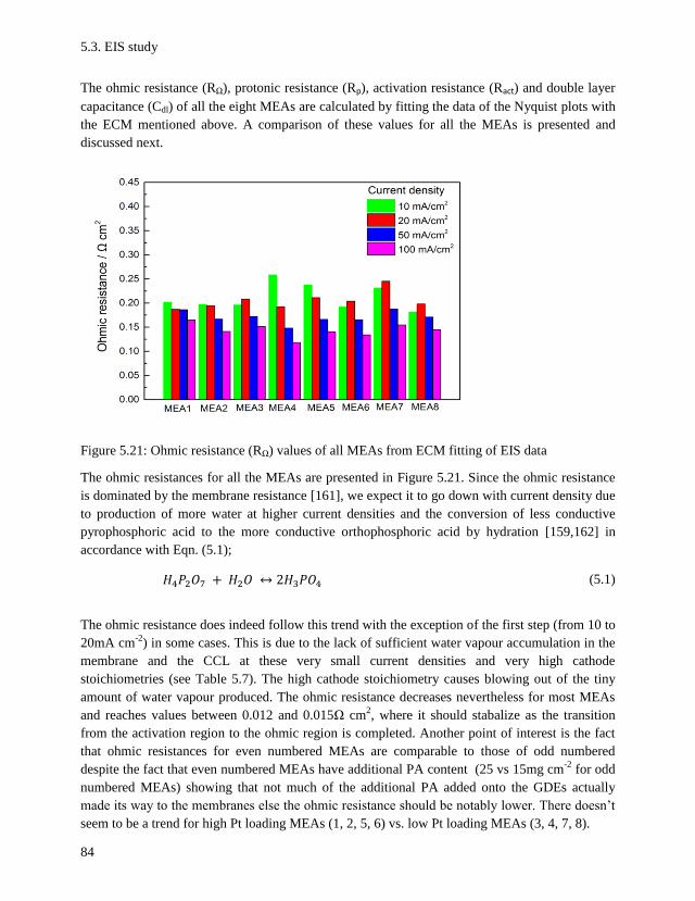
5.3. EIS study
84
The ohmic resistance (RΩ), protonic resistance (Rp), activation resistance (Ract) and double layer
capacitance (Cdl) of all the eight MEAs are calculated by fitting the data of the Nyquist plots with
the ECM mentioned above. A comparison of these values for all the MEAs is presented and
discussed next.
Figure 5.21: Ohmic resistance (RΩ) values of all MEAs from ECM fitting of EIS data
The ohmic resistances for all the MEAs are presented in Figure 5.21. Since the ohmic resistance
is dominated by the membrane resistance [161], we expect it to go down with current density due
to production of more water at higher current densities and the conversion of less conductive
pyrophosphoric acid to the more conductive orthophosphoric acid by hydration [159,162] in
accordance with Eqn. (5.1);
𝐻4𝑃2𝑂7 + 𝐻2𝑂 ↔ 2𝐻3𝑃𝑂4 (5.1)
The ohmic resistance does indeed follow this trend with the exception of the first step (from 10 to
20mA cm-2
) in some cases. This is due to the lack of sufficient water vapour accumulation in the
membrane and the CCL at these very small current densities and very high cathode
stoichiometries (see Table 5.7). The high cathode stoichiometry causes blowing out of the tiny
amount of water vapour produced. The ohmic resistance decreases nevertheless for most MEAs
and reaches values between 0.012 and 0.015Ω cm2, where it should stabalize as the transition
from the activation region to the ohmic region is completed. Another point of interest is the fact
that ohmic resistances for even numbered MEAs are comparable to those of odd numbered
despite the fact that even numbered MEAs have additional PA content (25 vs 15mg cm-2
for odd
numbered MEAs) showing that not much of the additional PA added onto the GDEs actually
made its way to the membranes else the ohmic resistance should be notably lower. There doesn’t
seem to be a trend for high Pt loading MEAs (1, 2, 5, 6) vs. low Pt loading MEAs (3, 4, 7, 8).
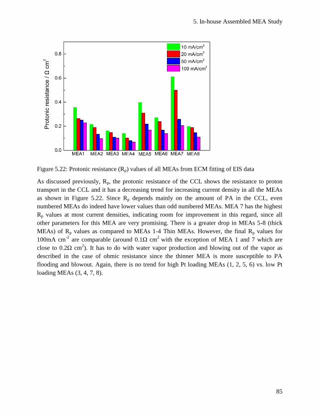
5. In-house Assembled MEA Study
85
Figure 5.22: Protonic resistance (Rp) values of all MEAs from ECM fitting of EIS data
As discussed previously, Rp, the protonic resistance of the CCL shows the resistance to proton
transport in the CCL and it has a decreasing trend for increasing current density in all the MEAs
as shown in Figure 5.22. Since Rp depends mainly on the amount of PA in the CCL, even
numbered MEAs do indeed have lower values than odd numbered MEAs. MEA 7 has the highest
Rp values at most current densities, indicating room for improvement in this regard, since all
other parameters for this MEA are very promising. There is a greater drop in MEAs 5-8 (thick
MEAs) of Rp values as compared to MEAs 1-4 Thin MEAs. However, the final Rp values for
100mA cm-2
are comparable (around 0.1Ω cm2
with the exception of MEA 1 and 7 which are
close to 0.2Ω cm2). It has to do with water vapor production and blowing out of the vapor as
described in the case of ohmic resistance since the thinner MEA is more susceptible to PA
flooding and blowout. Again, there is no trend for high Pt loading MEAs (1, 2, 5, 6) vs. low Pt
loading MEAs (3, 4, 7, 8).
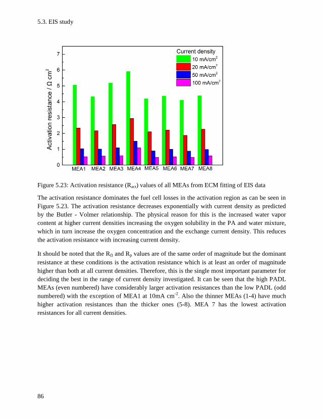
5.3. EIS study
86
Figure 5.23: Activation resistance (Ract) values of all MEAs from ECM fitting of EIS data
The activation resistance dominates the fuel cell losses in the activation region as can be seen in
Figure 5.23. The activation resistance decreases exponentially with current density as predicted
by the Butler - Volmer relationship. The physical reason for this is the increased water vapor
content at higher current densities increasing the oxygen solubility in the PA and water mixture,
which in turn increase the oxygen concentration and the exchange current density. This reduces
the activation resistance with increasing current density.
It should be noted that the RΩ and Rp values are of the same order of magnitude but the dominant
resistance at these conditions is the activation resistance which is at least an order of magnitude
higher than both at all current densities. Therefore, this is the single most important parameter for
deciding the best in the range of current density investigated. It can be seen that the high PADL
MEAs (even numbered) have considerably larger activation resistances than the low PADL (odd
numbered) with the exception of MEA1 at 10mA cm-2
. Also the thinner MEAs (1-4) have much
higher activation resistances than the thicker ones (5-8). MEA 7 has the lowest activation
resistances for all current densities.
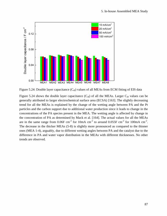
5. In-house Assembled MEA Study
87
Figure 5.24: Double layer capacitance (Cdl) values of all MEAs from ECM fitting of EIS data
Figure 5.24 shows the double layer capacitance (Cdl) of all the MEAs. Larger Cdl values can be
generally attributed to larger electrochemical surface area (ECSA) [163]. The slightly decreasing
trend for all the MEAs is explained by the change of the wetting angle between PA and the Pt
particles and the carbon support due to additional water production since it leads to change in the
concentrations of the PA species present in the MEA. The wetting angle is affected by change in
the concentration of PA as determined by Mack et al. [164]. The actual values for all the MEAs
are in the same range from 0.06F cm-2
for 10mA cm-2
to around 0.055F cm-2
for 100mA cm-2
.
The decrease in the thicker MEAs (5-8) is slightly more pronounced as compared to the thinner
ones (MEA 1-4), arguably, due to different wetting angles between PA and the catalyst due to the
difference in PA and water vapor distribution in the MEAs with different thicknesses. No other
trends are observed.
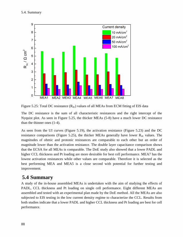
5.4. Summary
88
Figure 5.25: Total DC resistance (Rdc) values of all MEAs from ECM fitting of EIS data
The DC resistance is the sum of all characteristic resistances and the right intercept of the
Nyquist plot. As seen in Figure 5.25, the thicker MEAs (5-8) have a much lower DC resistance
than the thinner ones (1-4).
As seen from the UI curves (Figure 5.19), the activation resistance (Figure 5.23) and the DC
resistance comparisons (Figure 5.25), the thicker MEAs generally have lower Rdc values. The
magnitudes of ohmic and protonic resistances are comparable to each other but an order of
magnitude lower than the activation resistance. The double layer capacitance comparison shows
that the ECSA for all MEAs is comparable. The DoE study also showed that a lower PADL and
higher CCL thickness and Pt loading are more desirable for best cell performance. MEA7 has the
lowest activation resistances while other values are comparable. Therefore it is selected as the
best performing MEA and MEA5 is a close second with potential for further testing and
improvement.
5.4 Summary A study of the in-house assembled MEAs is undertaken with the aim of studying the effects of
PADL, CCL thickness and Pt loading on single cell performance. Eight different MEAs are
assembled and tested with an experimental plan made by the DoE method. All the MEAs are also
subjected to EIS testing in the low current density regime to characterize the CCL. Results from
both studies indicate that a lower PADL and higher CCL thickness and Pt loading are best for cell
performance.
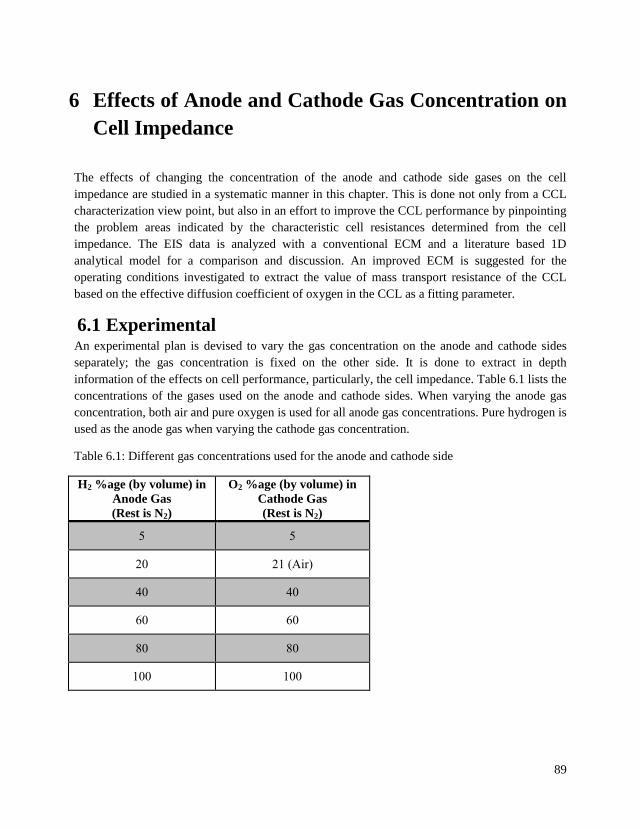
89
6 Effects of Anode and Cathode Gas Concentration on
Cell Impedance
The effects of changing the concentration of the anode and cathode side gases on the cell
impedance are studied in a systematic manner in this chapter. This is done not only from a CCL
characterization view point, but also in an effort to improve the CCL performance by pinpointing
the problem areas indicated by the characteristic cell resistances determined from the cell
impedance. The EIS data is analyzed with a conventional ECM and a literature based 1D
analytical model for a comparison and discussion. An improved ECM is suggested for the
operating conditions investigated to extract the value of mass transport resistance of the CCL
based on the effective diffusion coefficient of oxygen in the CCL as a fitting parameter.
6.1 Experimental An experimental plan is devised to vary the gas concentration on the anode and cathode sides
separately; the gas concentration is fixed on the other side. It is done to extract in depth
information of the effects on cell performance, particularly, the cell impedance. Table 6.1 lists the
concentrations of the gases used on the anode and cathode sides. When varying the anode gas
concentration, both air and pure oxygen is used for all anode gas concentrations. Pure hydrogen is
used as the anode gas when varying the cathode gas concentration.
Table 6.1: Different gas concentrations used for the anode and cathode side
H2 %age (by volume) in
Anode Gas
(Rest is N2)
O2 %age (by volume) in
Cathode Gas
(Rest is N2)
5 5
20 21 (Air)
40 40
60 60
80 80
100 100
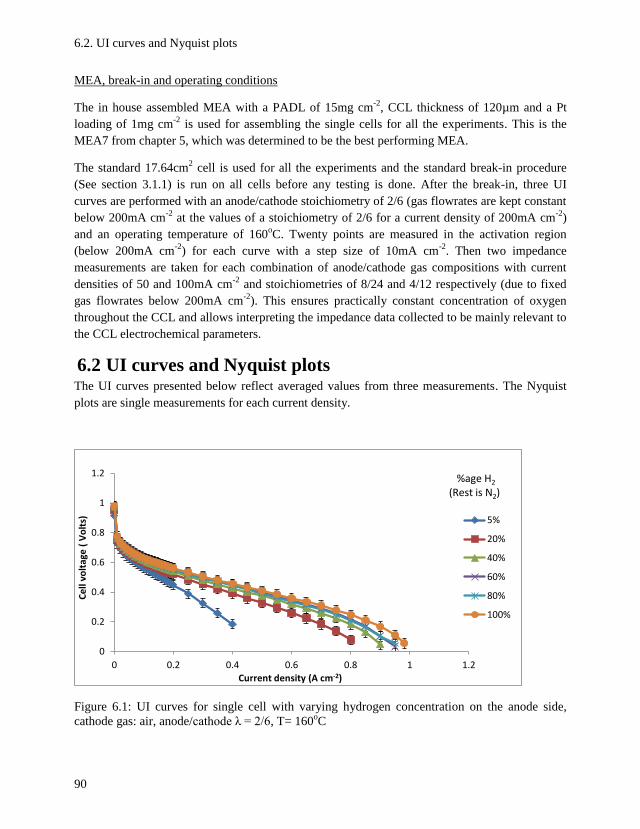
6.2. UI curves and Nyquist plots
90
MEA, break-in and operating conditions
The in house assembled MEA with a PADL of 15mg cm-2
, CCL thickness of 120µm and a Pt
loading of 1mg cm-2
is used for assembling the single cells for all the experiments. This is the
MEA7 from chapter 5, which was determined to be the best performing MEA.
The standard 17.64cm2 cell is used for all the experiments and the standard break-in procedure
(See section 3.1.1) is run on all cells before any testing is done. After the break-in, three UI
curves are performed with an anode/cathode stoichiometry of 2/6 (gas flowrates are kept constant
below 200mA cm-2
at the values of a stoichiometry of 2/6 for a current density of 200mA cm-2
)
and an operating temperature of 160oC. Twenty points are measured in the activation region
(below 200mA cm-2
) for each curve with a step size of 10mA cm-2
. Then two impedance
measurements are taken for each combination of anode/cathode gas compositions with current
densities of 50 and 100mA cm-2
and stoichiometries of 8/24 and 4/12 respectively (due to fixed
gas flowrates below 200mA cm-2
). This ensures practically constant concentration of oxygen
throughout the CCL and allows interpreting the impedance data collected to be mainly relevant to
the CCL electrochemical parameters.
6.2 UI curves and Nyquist plots The UI curves presented below reflect averaged values from three measurements. The Nyquist
plots are single measurements for each current density.
Figure 6.1: UI curves for single cell with varying hydrogen concentration on the anode side,
cathode gas: air, anode/cathode λ = 2/6, T= 160oC
0
0.2
0.4
0.6
0.8
1
1.2
0 0.2 0.4 0.6 0.8 1 1.2
Ce
ll vo
ltag
e (
Vo
lts)
Current density (A cm-2)
5%
20%
40%
60%
80%
100%
%age H2 (Rest is N2)
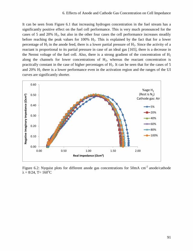
6. Effects of Anode and Cathode Gas Concentration on Cell Impedance
91
It can be seen from Figure 6.1 that increasing hydrogen concentration in the fuel stream has a
significantly positive effect on the fuel cell performance. This is very much pronounced for the
cases of 5 and 20% H2, but also in the other four cases the cell performance increases steadily
before reaching the peak values for 100% H2. This is explained by the fact that for a lower
percentage of H2 in the anode feed, there is a lower partial pressure of H2. Since the activity of a
reactant is proportional to its partial pressure in case of an ideal gas [165], there is a decrease in
the Nernst voltage of the fuel cell. Also, there is a strong gradient of the concentration of H2
along the channels for lower concentrations of H2, whereas the reactant concentration is
practically constant in the case of higher percentages of H2. It can be seen that for the cases of 5
and 20% H2 there is a lower performance even in the activation region and the ranges of the UI
curves are significantly shorter.
Figure 6.2: Nyquist plots for different anode gas concentrations for 50mA cm-2
anode/cathode
λ = 8/24, T= 160oC
0.00
0.10
0.20
0.30
0.40
0.50
0.60
0.00 0.50 1.00 1.50 2.00
Ne
gati
ve im
agin
ary
imp
ed
ance
(Ω
cm2 )
Real impedance (Ωcm2)
5%
20%
40%
60%
80%
100%
%age H2
(Rest is N2) Cathode gas: Air
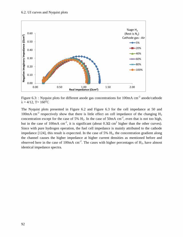
6.2. UI curves and Nyquist plots
92
Figure 6.3: : Nyquist plots for different anode gas concentrations for 100mA cm-2
anode/cathode
λ = 4/12, T= 160oC
The Nyquist plots presented in Figure 6.2 and Figure 6.3 for the cell impedance at 50 and
100mA cm-2
respectively show that there is little effect on cell impedance of the changing H2
concentration except for the case of 5% H2. In the case of 50mA cm-2
, even that is not too high,
but in the case of 100mA cm-2
, it is significant (about 0.3Ω cm2 higher than the other curves).
Since with pure hydrogen operation, the fuel cell impedance is mainly attributed to the cathode
impedance [124], this result is expeccted. In the case of 5% H2, the concentration gradient along
the channel causes the higher impedance at higher current densities as mentioned before and
observed here in the case of 100mA cm-2
. The cases with higher percentages of H2, have almost
identical impedance spectra.
0.00
0.10
0.20
0.30
0.40
0.50
0.60
0.00 0.50 1.00 1.50 2.00
Ne
gati
ve im
agin
ary
imp
ed
ance
(Ω
cm2 )
Real impedance (Ωcm2)
5%
20%
40%
60%
80%
100%
%age H2
(Rest is N2) Cathode gas : Air
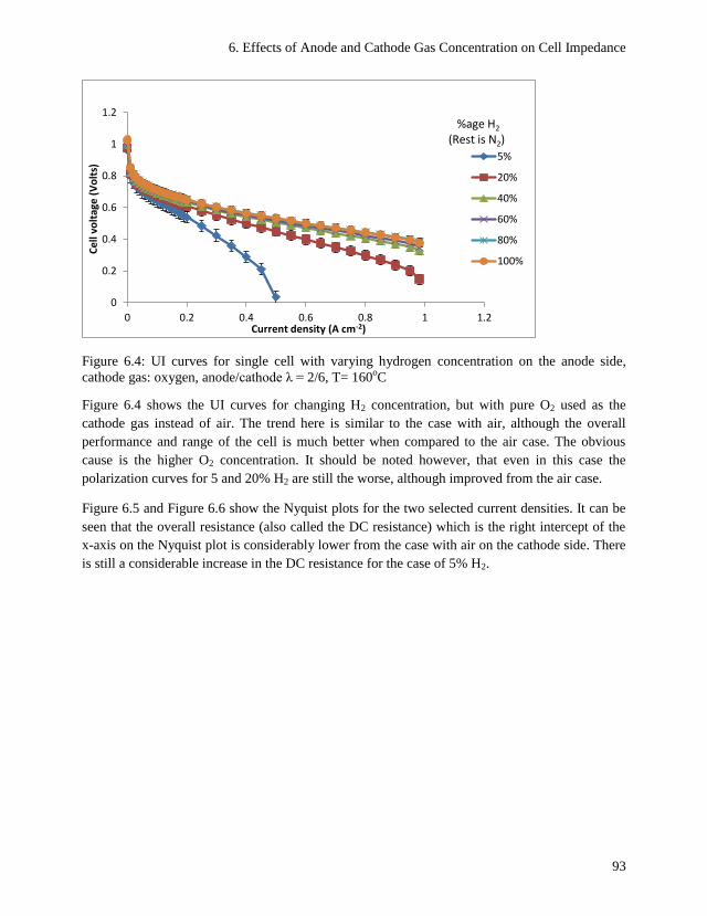
6. Effects of Anode and Cathode Gas Concentration on Cell Impedance
93
Figure 6.4: UI curves for single cell with varying hydrogen concentration on the anode side,
cathode gas: oxygen, anode/cathode λ = 2/6, T= 160oC
Figure 6.4 shows the UI curves for changing H2 concentration, but with pure O2 used as the
cathode gas instead of air. The trend here is similar to the case with air, although the overall
performance and range of the cell is much better when compared to the air case. The obvious
cause is the higher O2 concentration. It should be noted however, that even in this case the
polarization curves for 5 and 20% H2 are still the worse, although improved from the air case.
Figure 6.5 and Figure 6.6 show the Nyquist plots for the two selected current densities. It can be
seen that the overall resistance (also called the DC resistance) which is the right intercept of the
x-axis on the Nyquist plot is considerably lower from the case with air on the cathode side. There
is still a considerable increase in the DC resistance for the case of 5% H2.
0
0.2
0.4
0.6
0.8
1
1.2
0 0.2 0.4 0.6 0.8 1 1.2
Ce
ll vo
ltag
e (
Vo
lts)
Current density (A cm-2)
5%
20%
40%
60%
80%
100%
%age H2 (Rest is N2)
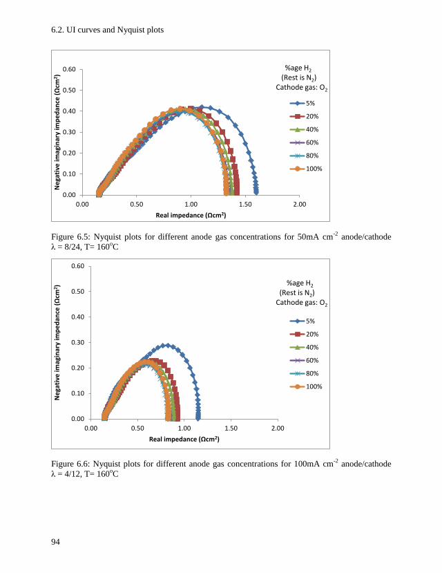
6.2. UI curves and Nyquist plots
94
Figure 6.5: Nyquist plots for different anode gas concentrations for 50mA cm-2
anode/cathode
λ = 8/24, T= 160oC
Figure 6.6: Nyquist plots for different anode gas concentrations for 100mA cm-2
anode/cathode
λ = 4/12, T= 160oC
0.00
0.10
0.20
0.30
0.40
0.50
0.60
0.00 0.50 1.00 1.50 2.00
Ne
gati
ve im
agin
ary
imp
ed
ance
(Ω
cm2 )
Real impedance (Ωcm2)
5%
20%
40%
60%
80%
100%
%age H2
(Rest is N2) Cathode gas: O2
0.00
0.10
0.20
0.30
0.40
0.50
0.60
0.00 0.50 1.00 1.50 2.00
Ne
gati
ve im
agin
ary
imp
ed
ance
(Ω
cm2)
Real impedance (Ωcm2)
5%
20%
40%
60%
80%
100%
%age H2 (Rest is N2) Cathode gas: O2
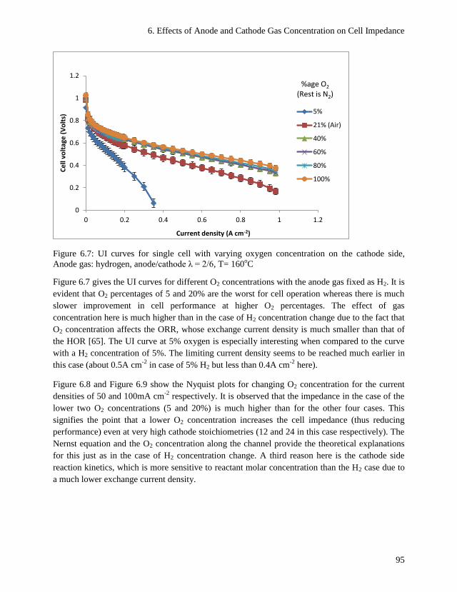
6. Effects of Anode and Cathode Gas Concentration on Cell Impedance
95
Figure 6.7: UI curves for single cell with varying oxygen concentration on the cathode side,
Anode gas: hydrogen, anode/cathode λ = 2/6, T= 160oC
Figure 6.7 gives the UI curves for different O2 concentrations with the anode gas fixed as H2. It is
evident that O2 percentages of 5 and 20% are the worst for cell operation whereas there is much
slower improvement in cell performance at higher O2 percentages. The effect of gas
concentration here is much higher than in the case of H2 concentration change due to the fact that
O2 concentration affects the ORR, whose exchange current density is much smaller than that of
the HOR [65]. The UI curve at 5% oxygen is especially interesting when compared to the curve
with a H2 concentration of 5%. The limiting current density seems to be reached much earlier in
this case (about 0.5A cm-2
in case of 5% H2 but less than 0.4A cm-2
here).
Figure 6.8 and Figure 6.9 show the Nyquist plots for changing O2 concentration for the current
densities of 50 and 100mA cm-2
respectively. It is observed that the impedance in the case of the
lower two O2 concentrations (5 and 20%) is much higher than for the other four cases. This
signifies the point that a lower O2 concentration increases the cell impedance (thus reducing
performance) even at very high cathode stoichiometries (12 and 24 in this case respectively). The
Nernst equation and the O2 concentration along the channel provide the theoretical explanations
for this just as in the case of H2 concentration change. A third reason here is the cathode side
reaction kinetics, which is more sensitive to reactant molar concentration than the H2 case due to
a much lower exchange current density.
0
0.2
0.4
0.6
0.8
1
1.2
0 0.2 0.4 0.6 0.8 1 1.2
Ce
ll vo
ltag
e (
Vo
lts)
Current density (A cm-2)
5%
21% (Air)
40%
60%
80%
100%
%age O2
(Rest is N2)
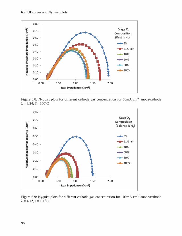
6.2. UI curves and Nyquist plots
96
Figure 6.8: Nyquist plots for different cathode gas concentration for 50mA cm-2
anode/cathode
λ = 8/24, T= 160oC
Figure 6.9: Nyquist plots for different cathode gas concentration for 100mA cm-2
anode/cathode
λ = 4/12, T= 160oC
0.00
0.10
0.20
0.30
0.40
0.50
0.60
0.70
0.80
0.00 0.50 1.00 1.50 2.00
Ne
gati
ve im
agin
ary
imp
ed
ance
(Ω
cm2)
Real impedance (Ωcm2)
5%
21% (air)
40%
60%
80%
100%
%age O2
Composition (Rest is N2)
0.00
0.10
0.20
0.30
0.40
0.50
0.60
0.70
0.80
0.00 0.50 1.00 1.50 2.00
Ne
gati
ve im
agin
ary
imp
ed
ance
(Ω
cm2 )
Real impedance (Ωcm2)
5%
21% (air)
40%
60%
80%
100%
%age O2
Composition (Balance is N2)
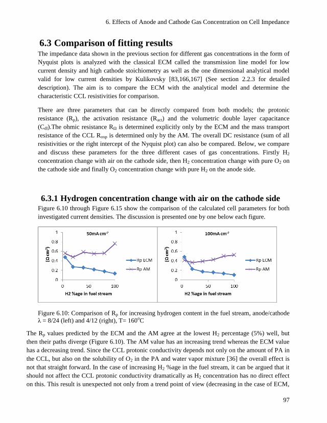
6. Effects of Anode and Cathode Gas Concentration on Cell Impedance
97
6.3 Comparison of fitting results The impedance data shown in the previous section for different gas concentrations in the form of
Nyquist plots is analyzed with the classical ECM called the transmission line model for low
current density and high cathode stoichiometry as well as the one dimensional analytical model
valid for low current densities by Kulikovsky [83,166,167] (See section 2.2.3 for detailed
description). The aim is to compare the ECM with the analytical model and determine the
characteristic CCL resistivities for comparison.
There are three parameters that can be directly compared from both models; the protonic
resistance (Rp), the activation resistance (Ract) and the volumetric double layer capacitance
(Cdl).The ohmic resistance RΩ is determined explicitly only by the ECM and the mass transport
resistance of the CCL Roxp is determined only by the AM. The overall DC resistance (sum of all
resistivities or the right intercept of the Nyquist plot) can also be compared. Below, we compare
and discuss these parameters for the three different cases of gas concentrations. Firstly H2
concentration change with air on the cathode side, then H2 concentration change with pure O2 on
the cathode side and finally O2 concentration change with pure H2 on the anode side.
6.3.1 Hydrogen concentration change with air on the cathode side Figure 6.10 through Figure 6.15 show the comparison of the calculated cell parameters for both
investigated current densities. The discussion is presented one by one below each figure.
Figure 6.10: Comparison of Rp for increasing hydrogen content in the fuel stream, anode/cathode
λ = 8/24 (left) and 4/12 (right), T= 160oC
The Rp values predicted by the ECM and the AM agree at the lowest H2 percentage (5%) well, but
then their paths diverge (Figure 6.10). The AM value has an increasing trend whereas the ECM value
has a decreasing trend. Since the CCL protonic conductivity depends not only on the amount of PA in
the CCL, but also on the solubility of O2 in the PA and water vapor mixture [36] the overall effect is
not that straight forward. In the case of increasing H2 %age in the fuel stream, it can be argued that it
should not affect the CCL protonic conductivity dramatically as H2 concentration has no direct effect
on this. This result is unexpected not only from a trend point of view (decreasing in the case of ECM,
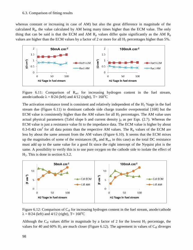
6.3. Comparison of fitting results
98
whereas constant or increasing in case of AM) but also the great difference in magnitude of the
calculated Rp, the value calculated by AM being many times higher than the ECM value. The only
thing that can be said is that the ECM and AM Rp values differ quite significantly as the AM Rp
values are higher than the ECM values by a factor of 2 or more for all H2 percentages higher than 5%.
Figure 6.11: Comparison of Ract for increasing hydrogen content in the fuel stream,
anode/cathode λ = 8/24 (left) and 4/12 (right), T= 160oC
The activation resistance trend is consistent and relatively independent of the H2 %age in the fuel
stream due (Figure 6.11) to dominant cathode side charge transfer overpotential [168] but the
ECM value is consistently higher than the AM values for all H2 percentages. The AM value uses
actual physical parameters (Tafel slope b and current density j0 as per Eqn. (2.7). Whereas the
ECM value is just a resistance value fit to the impedance data. The ECM value is higher by about
0.3-0.4Ω cm2 for all data points than the respective AM values. The Rp values of the ECM are
less by about the same amount from the AM values (Figure 6.10). It seems that the ECM mixes
up the magnitudes of some of the resistances (Rp and Ract in this case) as the total DC resistance
must add up to the same value for a good fit since the right intercept of the Nyquist plot is the
same. A possibility to verify this is to use pure oxygen on the cathode side to isolate the effect of
H2. This is done in section 6.3.2.
Figure 6.12: Comparison of Cdl for increasing hydrogen content in the fuel stream, anode/cathode
λ = 8/24 (left) and 4/12 (right), T= 160oC
Although the Cdl values differ in magnitude by a factor of 2 for the lowest H2 percentage, the
values for 40 and 60% H2 are much closer (Figure 6.12). The agreement in values of Cdl diverges
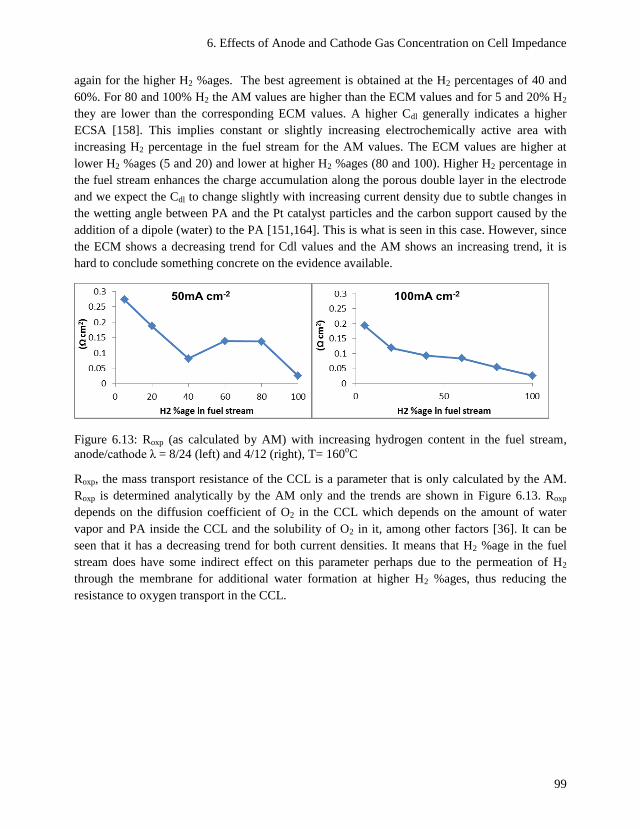
6. Effects of Anode and Cathode Gas Concentration on Cell Impedance
99
again for the higher H2 %ages. The best agreement is obtained at the H2 percentages of 40 and
60%. For 80 and 100% H2 the AM values are higher than the ECM values and for 5 and 20% H2
they are lower than the corresponding ECM values. A higher Cdl generally indicates a higher
ECSA [158]. This implies constant or slightly increasing electrochemically active area with
increasing H2 percentage in the fuel stream for the AM values. The ECM values are higher at
lower H2 %ages (5 and 20) and lower at higher H2 %ages (80 and 100). Higher H2 percentage in
the fuel stream enhances the charge accumulation along the porous double layer in the electrode
and we expect the Cdl to change slightly with increasing current density due to subtle changes in
the wetting angle between PA and the Pt catalyst particles and the carbon support caused by the
addition of a dipole (water) to the PA [151,164]. This is what is seen in this case. However, since
the ECM shows a decreasing trend for Cdl values and the AM shows an increasing trend, it is
hard to conclude something concrete on the evidence available.
Figure 6.13: Roxp (as calculated by AM) with increasing hydrogen content in the fuel stream,
anode/cathode λ = 8/24 (left) and 4/12 (right), T= 160oC
Roxp, the mass transport resistance of the CCL is a parameter that is only calculated by the AM.
Roxp is determined analytically by the AM only and the trends are shown in Figure 6.13. Roxp
depends on the diffusion coefficient of O2 in the CCL which depends on the amount of water
vapor and PA inside the CCL and the solubility of O2 in it, among other factors [36]. It can be
seen that it has a decreasing trend for both current densities. It means that H2 %age in the fuel
stream does have some indirect effect on this parameter perhaps due to the permeation of H2
through the membrane for additional water formation at higher H2 %ages, thus reducing the
resistance to oxygen transport in the CCL.
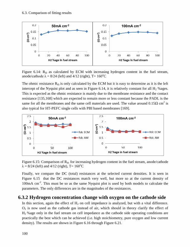
6.3. Comparison of fitting results
100
Figure 6.14: RΩ as calculated by ECM with increasing hydrogen content in the fuel stream,
anode/cathode λ = 8/24 (left) and 4/12 (right), T= 160oC
The ohmic resistance RΩ is only calculated by the ECM but it is easy to determine as it is the left
intercept of the Nyquist plot and as seen in Figure 6.14, it is relatively constant for all H2 %ages.
This is expected as the ohmic resistance is mainly due to the membrane resistance and the contact
resistance [135,168] which are expected to remain more or less constant because the PADL is the
same for all the membranes and the same cell materials are used. The value around 0.15Ω cm2 is
also typical for HT-PEFC single cells with PBI based membranes [169].
Figure 6.15: Comparison of Rdc for increasing hydrogen content in the fuel stream, anode/cathode
λ = 8/24 (left) and 4/12 (right), T= 160oC
Finally, we compare the DC (total) resistances at the selected current densities. It is seen in
Figure 6.15 that the DC resistances match very well, but more so at the current density of
100mA cm-2
. This must be so as the same Nyquist plot is used by both models to calculate the
parameters. The only differences are in the magnitudes of the resistances.
6.3.2 Hydrogen concentration change with oxygen on the cathode side In this section, again the effect of H2 on cell impedance is analyzed, but with a vital difference.
O2 is now used as the cathode gas instead of air, which should in theory clarify the effect of
H2 %age only in the fuel stream on cell impedance as the cathode side operating conditions are
practically the best which can be achieved (i.e. high stoichiometry, pure oxygen and low current
density). The results are shown in Figure 6.16 through Figure 6.21.
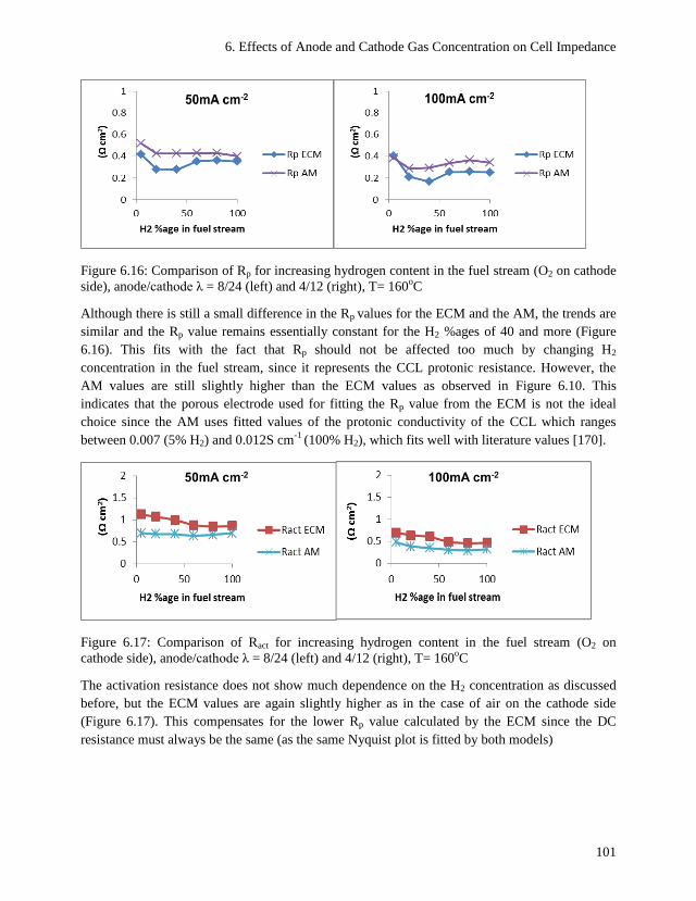
6. Effects of Anode and Cathode Gas Concentration on Cell Impedance
101
Figure 6.16: Comparison of Rp for increasing hydrogen content in the fuel stream (O2 on cathode
side), anode/cathode λ = 8/24 (left) and 4/12 (right), T= 160oC
Although there is still a small difference in the Rp values for the ECM and the AM, the trends are
similar and the Rp value remains essentially constant for the H2 %ages of 40 and more (Figure
6.16). This fits with the fact that Rp should not be affected too much by changing H2
concentration in the fuel stream, since it represents the CCL protonic resistance. However, the
AM values are still slightly higher than the ECM values as observed in Figure 6.10. This
indicates that the porous electrode used for fitting the Rp value from the ECM is not the ideal
choice since the AM uses fitted values of the protonic conductivity of the CCL which ranges
between 0.007 (5% H2) and 0.012S cm-1
(100% H2), which fits well with literature values [170].
Figure 6.17: Comparison of Ract for increasing hydrogen content in the fuel stream (O2 on
cathode side), anode/cathode λ = 8/24 (left) and 4/12 (right), T= 160oC
The activation resistance does not show much dependence on the H2 concentration as discussed
before, but the ECM values are again slightly higher as in the case of air on the cathode side
(Figure 6.17). This compensates for the lower Rp value calculated by the ECM since the DC
resistance must always be the same (as the same Nyquist plot is fitted by both models)
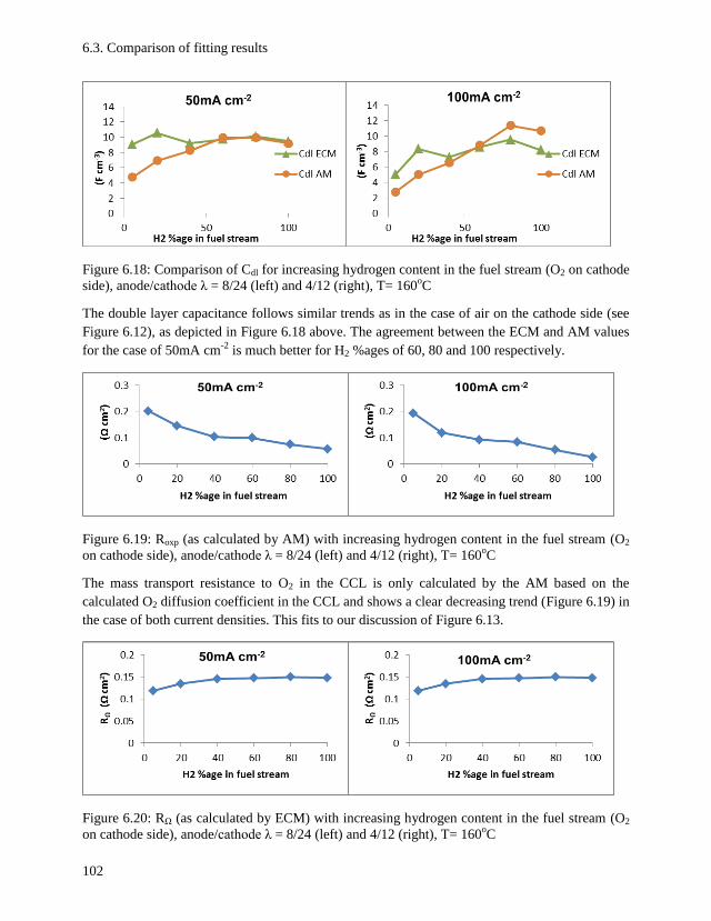
6.3. Comparison of fitting results
102
Figure 6.18: Comparison of Cdl for increasing hydrogen content in the fuel stream (O2 on cathode
side), anode/cathode λ = 8/24 (left) and 4/12 (right), T= 160oC
The double layer capacitance follows similar trends as in the case of air on the cathode side (see
Figure 6.12), as depicted in Figure 6.18 above. The agreement between the ECM and AM values
for the case of 50mA cm-2
is much better for H2 %ages of 60, 80 and 100 respectively.
Figure 6.19: Roxp (as calculated by AM) with increasing hydrogen content in the fuel stream (O2
on cathode side), anode/cathode λ = 8/24 (left) and 4/12 (right), T= 160oC
The mass transport resistance to O2 in the CCL is only calculated by the AM based on the
calculated O2 diffusion coefficient in the CCL and shows a clear decreasing trend (Figure 6.19) in
the case of both current densities. This fits to our discussion of Figure 6.13.
Figure 6.20: RΩ (as calculated by ECM) with increasing hydrogen content in the fuel stream (O2
on cathode side), anode/cathode λ = 8/24 (left) and 4/12 (right), T= 160oC
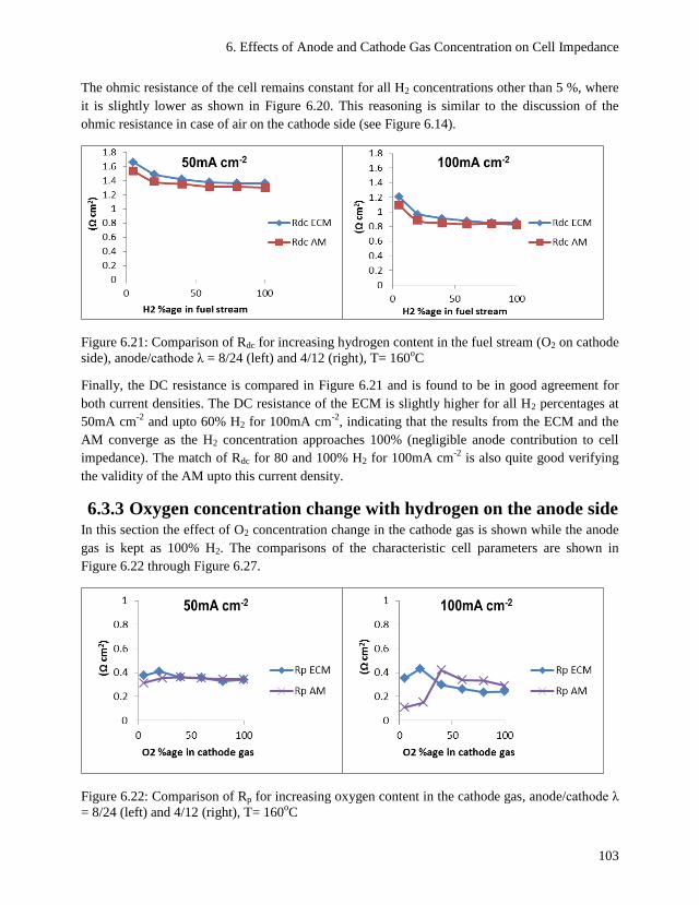
6. Effects of Anode and Cathode Gas Concentration on Cell Impedance
103
The ohmic resistance of the cell remains constant for all H2 concentrations other than 5 %, where
it is slightly lower as shown in Figure 6.20. This reasoning is similar to the discussion of the
ohmic resistance in case of air on the cathode side (see Figure 6.14).
Figure 6.21: Comparison of Rdc for increasing hydrogen content in the fuel stream (O2 on cathode
side), anode/cathode λ = 8/24 (left) and 4/12 (right), T= 160oC
Finally, the DC resistance is compared in Figure 6.21 and is found to be in good agreement for
both current densities. The DC resistance of the ECM is slightly higher for all H2 percentages at
50mA cm-2
and upto 60% H2 for 100mA cm-2
, indicating that the results from the ECM and the
AM converge as the H2 concentration approaches 100% (negligible anode contribution to cell
impedance). The match of Rdc for 80 and 100% H2 for 100mA cm-2
is also quite good verifying
the validity of the AM upto this current density.
6.3.3 Oxygen concentration change with hydrogen on the anode side In this section the effect of O2 concentration change in the cathode gas is shown while the anode
gas is kept as 100% H2. The comparisons of the characteristic cell parameters are shown in
Figure 6.22 through Figure 6.27.
Figure 6.22: Comparison of Rp for increasing oxygen content in the cathode gas, anode/cathode λ
= 8/24 (left) and 4/12 (right), T= 160oC
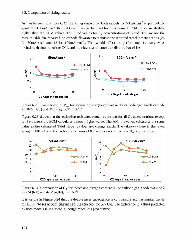
6.3. Comparison of fitting results
104
As can be seen in Figure 6.22, the Rp agreement for both models for 50mA cm-2
is particularly
good. For 100mA cm-2
, the first two points are far apart but then again the AM values are slightly
higher than the ECM values. The fitted values for O2 concentrations of 5 and 20% are not the
most reliable due to very high cathode flowrates to maintain the required stoichiometric ratios (24
for 50mA cm-2
and 12 for 100mA cm-2
). This would affect the performance in many ways
including drying out of the CCL and membrane and removal/redistribution of PA.
Figure 6.23: Comparison of Ract for increasing oxygen content in the cathode gas, anode/cathode
λ = 8/24 (left) and 4/12 (right), T= 160oC
Figure 6.23 shows that the activation resistance remains constant for all O2 concentrations except
for 5%, where the ECM calculates a much higher value. The AM , however, calculates the same
value as the calculated Tafel slope (b) does not change much. The takeaway here is that even
going to 100% O2 on the cathode side from 21% (air) does not reduce the Ract appreciably.
Figure 6.24: Comparison of Cdl for increasing oxygen content in the cathode gas, anode/cathode λ
= 8/24 (left) and 4/12 (right), T= 160oC
It is visible in Figure 6.24 that the double layer capacitance is comparable and has similar trends
for all O2 %ages at both current densities (except for 5% O2). The difference in values predicted
by both models is still there, although much less pronounced.
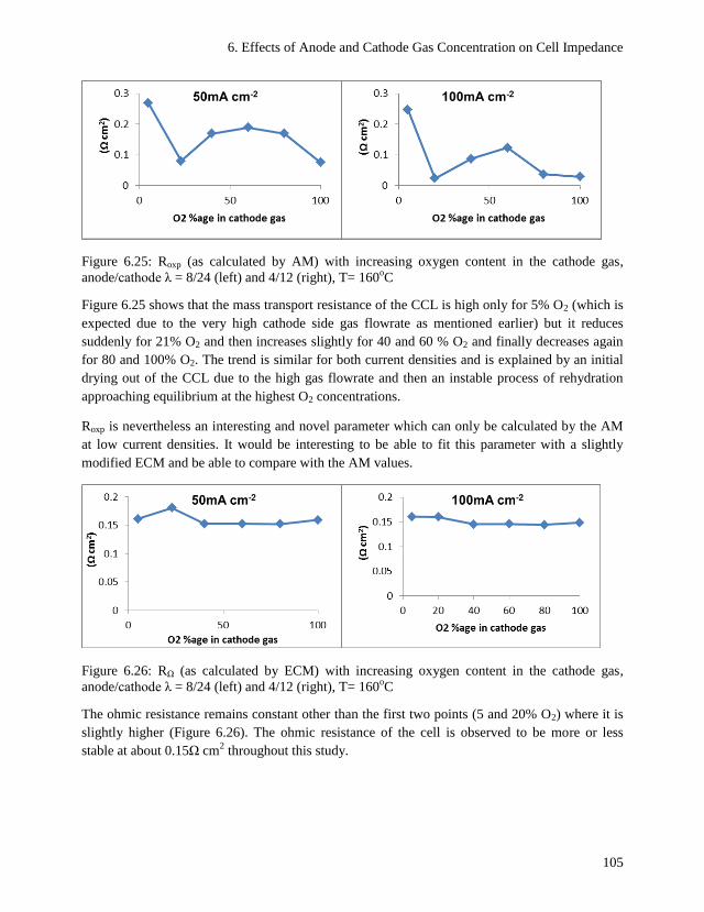
6. Effects of Anode and Cathode Gas Concentration on Cell Impedance
105
Figure 6.25: Roxp (as calculated by AM) with increasing oxygen content in the cathode gas,
anode/cathode λ = 8/24 (left) and 4/12 (right), T= 160oC
Figure 6.25 shows that the mass transport resistance of the CCL is high only for 5% O2 (which is
expected due to the very high cathode side gas flowrate as mentioned earlier) but it reduces
suddenly for 21% O2 and then increases slightly for 40 and 60 % O2 and finally decreases again
for 80 and 100% O2. The trend is similar for both current densities and is explained by an initial
drying out of the CCL due to the high gas flowrate and then an instable process of rehydration
approaching equilibrium at the highest O2 concentrations.
Roxp is nevertheless an interesting and novel parameter which can only be calculated by the AM
at low current densities. It would be interesting to be able to fit this parameter with a slightly
modified ECM and be able to compare with the AM values.
Figure 6.26: RΩ (as calculated by ECM) with increasing oxygen content in the cathode gas,
anode/cathode λ = 8/24 (left) and 4/12 (right), T= 160oC
The ohmic resistance remains constant other than the first two points (5 and 20% O2) where it is
slightly higher (Figure 6.26). The ohmic resistance of the cell is observed to be more or less
stable at about 0.15Ω cm2 throughout this study.
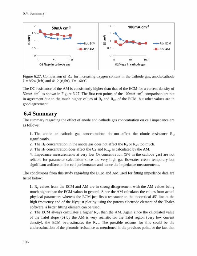
6.4. Summary
106
Figure 6.27: Comparison of Rdc for increasing oxygen content in the cathode gas, anode/cathode
λ = 8/24 (left) and 4/12 (right), T= 160oC
The DC resistance of the AM is consistently higher than that of the ECM for a current density of
50mA cm-2
as shown in Figure 6.27. The first two points of the 100mA cm-2
comparison are not
in agreement due to the much higher values of Rp and Ract of the ECM, but other values are in
good agreement.
6.4 Summary The summary regarding the effect of anode and cathode gas concentration on cell impedance are
as follows:
1. The anode or cathode gas concentrations do not affect the ohmic resistance RΩ
significantly.
2. The H2 concentration in the anode gas does not affect the Rp or Ract too much.
3. The H2 concentration does affect the Cdl and Roxp as calculated by the AM.
4. Impedance measurements at very low O2 concentration (5% in the cathode gas) are not
reliable for parameter calculation since the very high gas flowrates create temporary but
significant artifacts in the cell performance and hence the impedance measurements.
The conclusions from this study regarding the ECM and AM used for fitting impedance data are
listed below:
1. Rp values from the ECM and AM are in strong disagreement with the AM values being
much higher than the ECM values in general. Since the AM calculates the values from actual
physical parameters whereas the ECM just fits a resistance to the theoretical 45o line at the
high frequency end of the Nyquist plot by using the porous electrode element of the Thales
software, a better fitting element can be used.
2. The ECM always calculates a higher Ract than the AM. Again since the calculated value
of the Tafel slope (b) by the AM is very realistic for the Tafel region (very low current
density), the ECM overestimates the Ract. The possible reasons for this could be the
underestimation of the protonic resistance as mentioned in the previous point, or the fact that
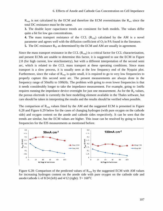
6. Effects of Anode and Cathode Gas Concentration on Cell Impedance
107
Roxp is not calculated by the ECM and therefore the ECM overestimates the Ract since the
total DC resistance must be the same.
3. The double layer capacitance trends are consistent for both models. The values differ
quite a bit for low gas concentrations.
4. The mass transport resistance of the CCL (Roxp) calculated by the AM is a novel
parameter and agrees well with the diffusion coefficient of O2 in PA found in the literature.
5. The DC resistance Rdc as determined by the ECM and AM are usually in agreement.
Since the mass transport resistance in the CCL (Roxp) is a critical factor for CCL characterization,
and present ECMs are unable to determine this factor, it is suggested to use the ECM in Figure
2.8 (for high current, low stoichiometry), but with a different interpretation of the second semi
arc, which is related to the CCL mass transport at these operating conditions. Since mass
transport is a slow process, it is usually seen at the low frequency end of the Nyquist plot.
Furthermore, since the value of Roxp is quite small, it is required to go to very low frequencies to
properly capture this second semi arc. The present measurements are always done in the
frequency range of 50mHz to 100kHz. The problem with going to even lower frequencies is that
it needs considerably longer to take the impedance measurement. For example, going to 1mHz
requires running the impedance device overnight for just one measurement. As for the Rp values,
the porous electrode is currently the best modelling element available in the Thales software, but
care should be taken in interpreting the results and the results should be verified when possible.
The comparison of Roxp values fitted by the AM and the suggested ECM is presented in Figure
6.28 and Figure 6.29 below for the cases of changing hydrogen (with pure oxygen on the cathode
side) and oxygen content on the anode and cathode sides respectively. It can be seen that the
trends are similar, but the ECM values are higher. This issue can be resolved by going to lower
frequencies for the EIS measurements as mentioned before.
Figure 6.28: Comparison of the predicted values of Roxp by the suggested ECM with AM values
for increasing hydrogen content on the anode side with pure oxygen on the cathode side and
anode/cathode λ of 8/24 (left) and 4/12 (right). T= 160oC

6.4. Summary
108
Figure 6.29: Comparison of the predicted values of Roxp by the suggested ECM with AM values
for increasing oxygen content on the cathode side with hydrogen on the anode side and
anode/cathode λ of 8/24 (left) and 4/12 (right). T= 160oC
109
7 Accelerated Degradation Study
Degradation of materials and components is a very important issue in PEFCs. It is especially so
for the HT-PEFC as the higher operating temperature causes much faster degradation of cell
components. Not many comprehensive publications on the degradation of the HT-PEFCs are
found in the literature; for example, one such detailed work was published by Schmidt et al [171].
Standardization of accelerated stress tests (AST) and degradation protocols for HT-PEFCs is also
an important task for better comparisons between different groups. It is hoped that this chapter
will be a small but significant step in this direction.
7.1 Experimental A degradation testing plan is devised for five stressors for accelerated degradation of the
HT-PEFC MEAs. The standard 17.64cm2 cell is used for testing all MEAs and the standard
break-in procedure is run on the cells before any testing (see section 3.1). The BOL UI curves are
taken immediately after the break-in procedure. Then BOL impedance and CV measurements are
performed to obtain the BOL characteristic parameters and ECSA of the fuel cell. Then each cell
is run for 100 hours of uninterrupted operation on a particular stressor. At the end of testing, the
EOL UI curves are taken and also EOL Impedance and CV measurements are performed. When
taking UI curves, always three curves are taken one after the other and averaged. Impedance and
CV measurements are always performed with similar settings to maintain comparability. The
impedance measurements are always taken with an anode/cathode stoichiometry of 2/2 at 200mA
cm-2
. Stable conditions are ensured before taking the impedance measurements. The impedance
data is analyzed with a standard ECM for fitting high current density impedance which has two
parallel R/CPE combinations to model the two semi arcs expected in the data. The first semi arc
represents the activation losses, whereas the second one represents the mass transfer losses of the
fuel cell. Since with pure H2 operation, the anode losses can be neglected, these losses are mainly
affiliated with the cathode side.
Three commercially available HT-PEFC MEAs from Advent technologies®
are used for this
campaign. Advent technologies®
recently acquired the patented materials and manufacturing
processes of the Celtec®
PW1100 HT-PEFC MEA from BASF. This MEA is now available
under the product series APM of Advent. The MEAs used for this campaign along with relevant
information are shown in Table 7.1.

7.1. Experimental
110
Table 7.1: List of commercial MEAs from Advent technologies®
used for degradation testing
Serial #
Product
MEA series
name
Membrane type GDE type
1 AAM TPS Advent GDE
2 ABM TPS BASF GDE
3 APM PBI BASF GDE
The TPS type membrane is a specialized membrane by Advent which consists of pyridine type
structures around a stable polymer. The PBI type membrane is the one previously available under
the name of Celtec®
by BASF and now by Advent under the MEA series APM. This PBI
membrane is doped with PA using the sol-gel technique previously patented by BASF and now
by Advent. The PBI membrane has a high PA content (34mg cm-2
± 4) [172] and thus higher
protonic conductivity than the TPS membrane (0.1Ω-1
cm-1
vs. 0.08Ω-1
cm-1
) [127], which is more
robust for harsh operating conditions. The BASF carbon cloth GDE is also now used by Advent
in the product series ABM and APM respectively. In effect, the AAM series is the same as the
previously known Advent TPS MEA; the APM series is the same as the Celtec®
PW1100 MEA
from BASF previously, while the ABM series is a new mixture of both MEAs with the
membrane of the former and the GDE of the latter [127].
7.1.1 Stressors and their implementation Five different stressors are used to test the MEAs. The stressors and their respective ranges or
values along with implementation mode and dominant degradation modes are given in Table 7.2.
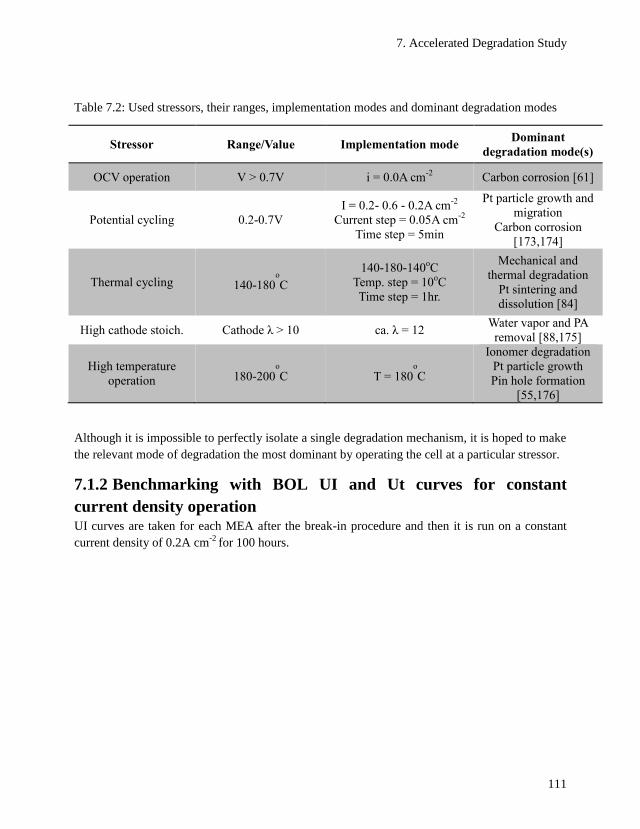
7. Accelerated Degradation Study
111
Table 7.2: Used stressors, their ranges, implementation modes and dominant degradation modes
Stressor Range/Value Implementation mode Dominant
degradation mode(s)
OCV operation V > 0.7V i = 0.0A cm-2
Carbon corrosion [61]
Potential cycling 0.2-0.7V
I = 0.2- 0.6 - 0.2A cm-2
Current step = 0.05A cm-2
Time step = 5min
Pt particle growth and
migration
Carbon corrosion
[173,174]
Thermal cycling 140-180o
C
140-180-140oC
Temp. step = 10oC
Time step = 1hr.
Mechanical and
thermal degradation
Pt sintering and
dissolution [84]
High cathode stoich. Cathode λ > 10 ca. λ = 12 Water vapor and PA
removal [88,175]
High temperature
operation 180-200o
C T = 180o
C
Ionomer degradation
Pt particle growth
Pin hole formation
[55,176]
Although it is impossible to perfectly isolate a single degradation mechanism, it is hoped to make
the relevant mode of degradation the most dominant by operating the cell at a particular stressor.
7.1.2 Benchmarking with BOL UI and Ut curves for constant
current density operation UI curves are taken for each MEA after the break-in procedure and then it is run on a constant
current density of 0.2A cm-2
for 100 hours.
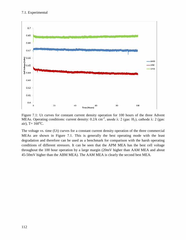
7.1. Experimental
112
Figure 7.1: Ut curves for constant current density operation for 100 hours of the three Advent
MEAs. Operating conditions: current density: 0.2A cm-2
, anode λ: 2 (gas: H2), cathode λ: 2 (gas:
air), T= 160oC.
The voltage vs. time (Ut) curves for a constant current density operation of the three commercial
MEAs are shown in Figure 7.1. This is generally the best operating mode with the least
degradation and therefore can be used as a benchmark for comparison with the harsh operating
conditions of different stressors. It can be seen that the APM MEA has the best cell voltage
throughout the 100 hour operation by a large margin (20mV higher than AAM MEA and about
45-50mV higher than the ABM MEA). The AAM MEA is clearly the second best MEA.
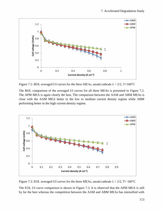
7. Accelerated Degradation Study
113
Figure 7.2: BOL averaged UI curves for the three MEAs, anode/cathode λ = 2/2, T=160°C
The BOL comparison of the averaged UI curves for all three MEAs is presented in Figure 7.2.
The APM MEA is again clearly the best. The comparison between the AAM and ABM MEAs is
close with the AAM MEA better in the low to medium current density regime while ABM
performing better in the high current density regime.
Figure 7.3: EOL averaged UI curves for the three MEAs, anode/cathode λ = 2/2, T= 160°C
The EOL UI curve comparison is shown in Figure 7.3. It is observed that the APM MEA is still
by far the best whereas the competition between the AAM and ABM MEAs has intensified with
0
0.2
0.4
0.6
0.8
1
1.2
0 0.2 0.4 0.6 0.8 1
Ce
ll vo
ltag
e (
Vo
lts)
Current density (A cm-2)
AAM
ABM
APM
0
0.2
0.4
0.6
0.8
1
1.2
0 0.1 0.2 0.3 0.4 0.5 0.6 0.7 0.8 0.9
Ce
ll vo
ltag
e (
volt
s)
Current density (A cm-2)
AAM
ABM
APM
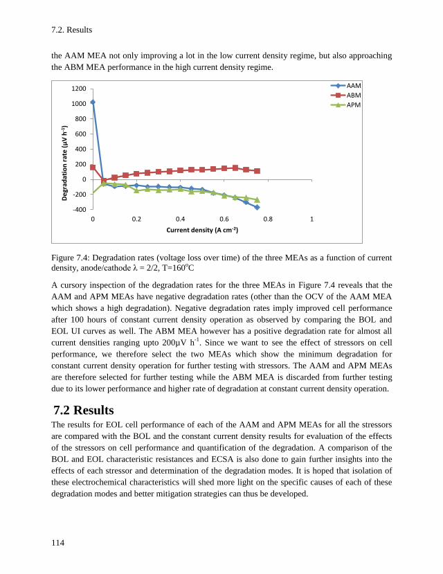
7.2. Results
114
the AAM MEA not only improving a lot in the low current density regime, but also approaching
the ABM MEA performance in the high current density regime.
Figure 7.4: Degradation rates (voltage loss over time) of the three MEAs as a function of current
density, anode/cathode λ = 2/2, T=160oC
A cursory inspection of the degradation rates for the three MEAs in Figure 7.4 reveals that the
AAM and APM MEAs have negative degradation rates (other than the OCV of the AAM MEA
which shows a high degradation). Negative degradation rates imply improved cell performance
after 100 hours of constant current density operation as observed by comparing the BOL and
EOL UI curves as well. The ABM MEA however has a positive degradation rate for almost all
current densities ranging upto 200µV h-1
. Since we want to see the effect of stressors on cell
performance, we therefore select the two MEAs which show the minimum degradation for
constant current density operation for further testing with stressors. The AAM and APM MEAs
are therefore selected for further testing while the ABM MEA is discarded from further testing
due to its lower performance and higher rate of degradation at constant current density operation.
7.2 Results The results for EOL cell performance of each of the AAM and APM MEAs for all the stressors
are compared with the BOL and the constant current density results for evaluation of the effects
of the stressors on cell performance and quantification of the degradation. A comparison of the
BOL and EOL characteristic resistances and ECSA is also done to gain further insights into the
effects of each stressor and determination of the degradation modes. It is hoped that isolation of
these electrochemical characteristics will shed more light on the specific causes of each of these
degradation modes and better mitigation strategies can thus be developed.
-400
-200
0
200
400
600
800
1000
1200
0 0.2 0.4 0.6 0.8 1
De
grad
atio
n r
ate
(μ
V h
-1)
Current density (A cm-2)
AAM
ABM
APM
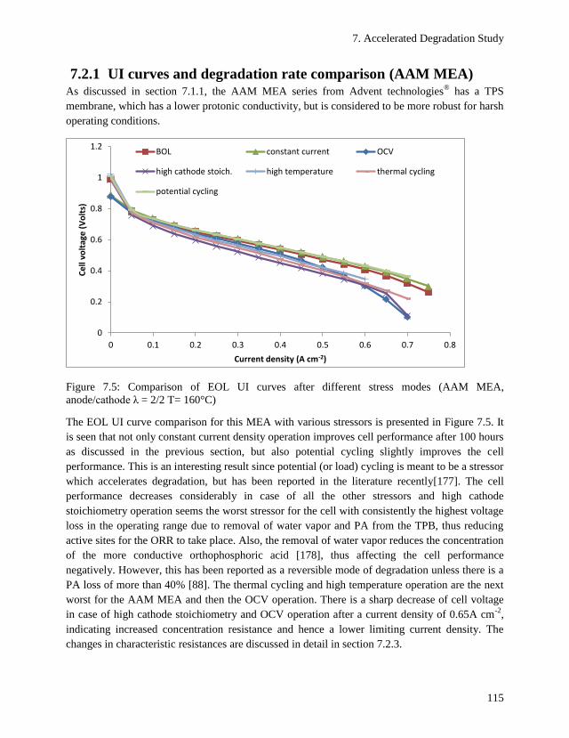
7. Accelerated Degradation Study
115
7.2.1 UI curves and degradation rate comparison (AAM MEA) As discussed in section 7.1.1, the AAM MEA series from Advent technologies
® has a TPS
membrane, which has a lower protonic conductivity, but is considered to be more robust for harsh
operating conditions.
Figure 7.5: Comparison of EOL UI curves after different stress modes (AAM MEA,
anode/cathode λ = 2/2 T= 160°C)
The EOL UI curve comparison for this MEA with various stressors is presented in Figure 7.5. It
is seen that not only constant current density operation improves cell performance after 100 hours
as discussed in the previous section, but also potential cycling slightly improves the cell
performance. This is an interesting result since potential (or load) cycling is meant to be a stressor
which accelerates degradation, but has been reported in the literature recently[177]. The cell
performance decreases considerably in case of all the other stressors and high cathode
stoichiometry operation seems the worst stressor for the cell with consistently the highest voltage
loss in the operating range due to removal of water vapor and PA from the TPB, thus reducing
active sites for the ORR to take place. Also, the removal of water vapor reduces the concentration
of the more conductive orthophosphoric acid [178], thus affecting the cell performance
negatively. However, this has been reported as a reversible mode of degradation unless there is a
PA loss of more than 40% [88]. The thermal cycling and high temperature operation are the next
worst for the AAM MEA and then the OCV operation. There is a sharp decrease of cell voltage
in case of high cathode stoichiometry and OCV operation after a current density of 0.65A cm-2
,
indicating increased concentration resistance and hence a lower limiting current density. The
changes in characteristic resistances are discussed in detail in section 7.2.3.
0
0.2
0.4
0.6
0.8
1
1.2
0 0.1 0.2 0.3 0.4 0.5 0.6 0.7 0.8
Ce
ll vo
ltag
e (
Vo
lts)
Current density (A cm-2)
BOL constant current OCV
high cathode stoich. high temperature thermal cycling
potential cycling
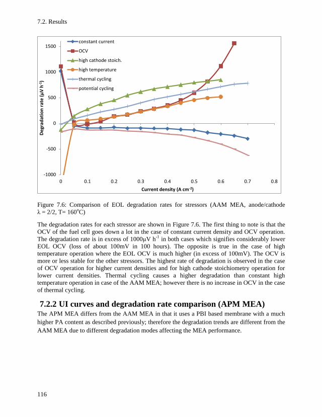
7.2. Results
116
Figure 7.6: Comparison of EOL degradation rates for stressors (AAM MEA, anode/cathode
λ = 2/2, T= 160oC)
The degradation rates for each stressor are shown in Figure 7.6. The first thing to note is that the
OCV of the fuel cell goes down a lot in the case of constant current density and OCV operation.
The degradation rate is in excess of 1000μV h-1
in both cases which signifies considerably lower
EOL OCV (loss of about 100mV in 100 hours). The opposite is true in the case of high
temperature operation where the EOL OCV is much higher (in excess of 100mV). The OCV is
more or less stable for the other stressors. The highest rate of degradation is observed in the case
of OCV operation for higher current densities and for high cathode stoichiometry operation for
lower current densities. Thermal cycling causes a higher degradation than constant high
temperature operation in case of the AAM MEA; however there is no increase in OCV in the case
of thermal cycling.
7.2.2 UI curves and degradation rate comparison (APM MEA) The APM MEA differs from the AAM MEA in that it uses a PBI based membrane with a much
higher PA content as described previously; therefore the degradation trends are different from the
AAM MEA due to different degradation modes affecting the MEA performance.
-1000
-500
0
500
1000
1500
0 0.1 0.2 0.3 0.4 0.5 0.6 0.7 0.8
De
grad
atio
n r
ate
(μ
V h
-1)
Current density (A cm-2)
constant current
OCV
high cathode stoich.
high temperature
thermal cycling
potential cycling
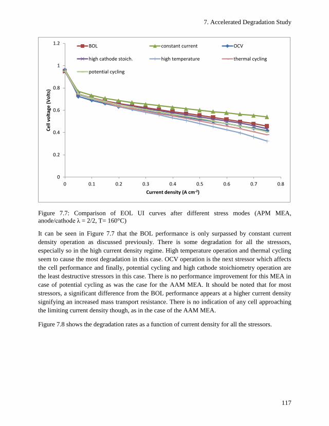
7. Accelerated Degradation Study
117
Figure 7.7: Comparison of EOL UI curves after different stress modes (APM MEA,
anode/cathode λ = 2/2, T= 160°C)
It can be seen in Figure 7.7 that the BOL performance is only surpassed by constant current
density operation as discussed previously. There is some degradation for all the stressors,
especially so in the high current density regime. High temperature operation and thermal cycling
seem to cause the most degradation in this case. OCV operation is the next stressor which affects
the cell performance and finally, potential cycling and high cathode stoichiometry operation are
the least destructive stressors in this case. There is no performance improvement for this MEA in
case of potential cycling as was the case for the AAM MEA. It should be noted that for most
stressors, a significant difference from the BOL performance appears at a higher current density
signifying an increased mass transport resistance. There is no indication of any cell approaching
the limiting current density though, as in the case of the AAM MEA.
Figure 7.8 shows the degradation rates as a function of current density for all the stressors.
0
0.2
0.4
0.6
0.8
1
1.2
0 0.1 0.2 0.3 0.4 0.5 0.6 0.7 0.8
Ce
ll vo
ltag
e (
Vo
lts)
Current density (A cm-2)
BOL constant current OCV
high cathode stoich. high temperature thermal cycling
potential cycling
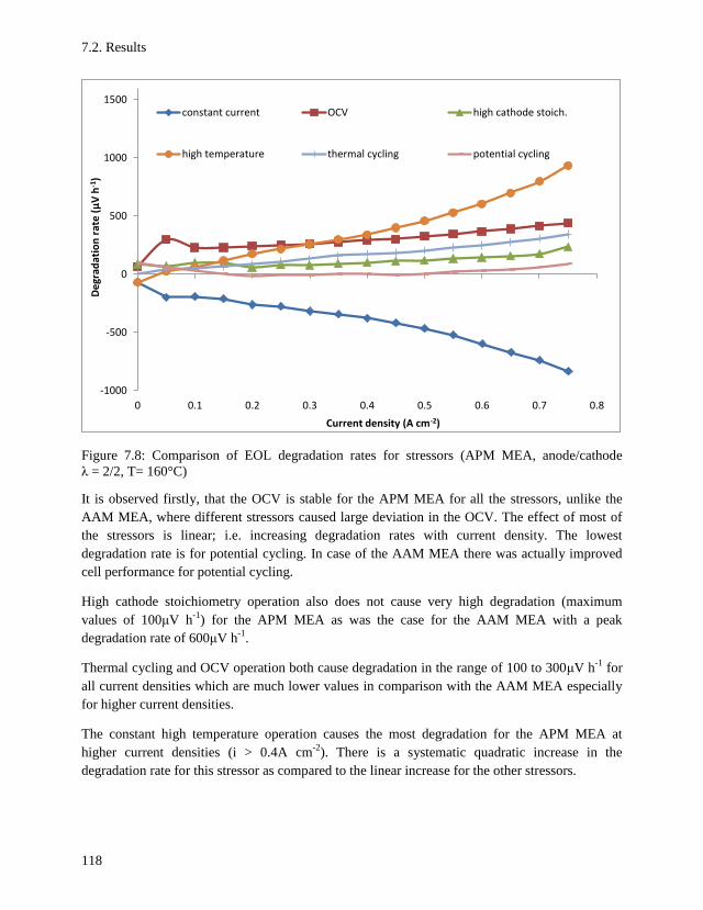
7.2. Results
118
Figure 7.8: Comparison of EOL degradation rates for stressors (APM MEA, anode/cathode
λ = 2/2, T= 160°C)
It is observed firstly, that the OCV is stable for the APM MEA for all the stressors, unlike the
AAM MEA, where different stressors caused large deviation in the OCV. The effect of most of
the stressors is linear; i.e. increasing degradation rates with current density. The lowest
degradation rate is for potential cycling. In case of the AAM MEA there was actually improved
cell performance for potential cycling.
High cathode stoichiometry operation also does not cause very high degradation (maximum
values of 100μV h-1
) for the APM MEA as was the case for the AAM MEA with a peak
degradation rate of 600μV h-1
.
Thermal cycling and OCV operation both cause degradation in the range of 100 to 300μV h-1
for
all current densities which are much lower values in comparison with the AAM MEA especially
for higher current densities.
The constant high temperature operation causes the most degradation for the APM MEA at
higher current densities (i > 0.4A cm-2
). There is a systematic quadratic increase in the
degradation rate for this stressor as compared to the linear increase for the other stressors.
-1000
-500
0
500
1000
1500
0 0.1 0.2 0.3 0.4 0.5 0.6 0.7 0.8
De
grad
atio
n r
ate
(μ
V h
-1)
Current density (A cm-2)
constant current OCV high cathode stoich.
high temperature thermal cycling potential cycling
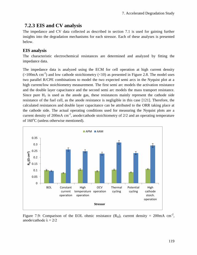
7. Accelerated Degradation Study
119
7.2.3 EIS and CV analysis The impedance and CV data collected as described in section 7.1 is used for gaining further
insights into the degradation mechanisms for each stressor. Each of these analyses is presented
below.
EIS analysis
The characteristic electrochemical resistances are determined and analyzed by fitting the
impedance data.
The impedance data is analyzed using the ECM for cell operation at high current density
(>100mA cm-2
) and low cathode stoichiometry (<10) as presented in Figure 2.8. The model uses
two parallel R/CPE combinations to model the two expected semi arcs in the Nyquist plot at a
high current/low stoichiometry measurement. The first semi arc models the activation resistance
and the double layer capacitance and the second semi arc models the mass transport resistance.
Since pure H2 is used as the anode gas, these resistances mainly represent the cathode side
resistance of the fuel cell, as the anode resistance is negligible in this case [121]. Therefore, the
calculated resistances and double layer capacitance can be attributed to the ORR taking place at
the cathode side. The actual operating conditions used for measuring the Nyquist plots are a
current density of 200mA cm-2
, anode/cathode stoichiometry of 2/2 and an operating temperature
of 160oC (unless otherwise mentioned).
Figure 7.9: Comparison of the EOL ohmic resistance (RΩ), current density = 200mA cm-2
,
anode/cathode λ = 2/2
0
0.05
0.1
0.15
0.2
0.25
0.3
0.35
BOL Constantcurrent
operation
Hightemperature
operation
OCVoperation
Thermalcycling
Potentialcycling
Highcathodestoich.
operation
RΩ
(Ω c
m2)
Stressor
APM AAM
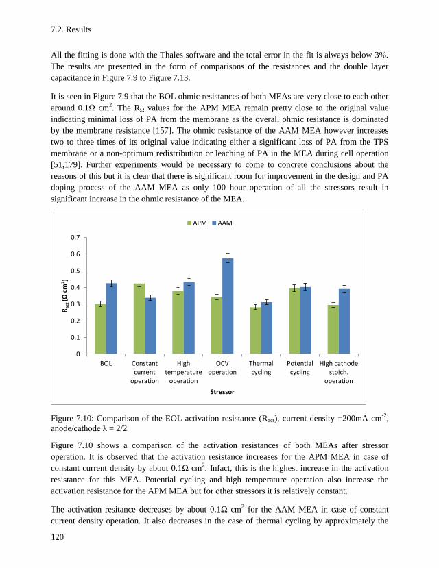
7.2. Results
120
All the fitting is done with the Thales software and the total error in the fit is always below 3%.
The results are presented in the form of comparisons of the resistances and the double layer
capacitance in Figure 7.9 to Figure 7.13.
It is seen in Figure 7.9 that the BOL ohmic resistances of both MEAs are very close to each other
around 0.1Ω cm2. The RΩ values for the APM MEA remain pretty close to the original value
indicating minimal loss of PA from the membrane as the overall ohmic resistance is dominated
by the membrane resistance [157]. The ohmic resistance of the AAM MEA however increases
two to three times of its original value indicating either a significant loss of PA from the TPS
membrane or a non-optimum redistribution or leaching of PA in the MEA during cell operation
[51,179]. Further experiments would be necessary to come to concrete conclusions about the
reasons of this but it is clear that there is significant room for improvement in the design and PA
doping process of the AAM MEA as only 100 hour operation of all the stressors result in
significant increase in the ohmic resistance of the MEA.
Figure 7.10: Comparison of the EOL activation resistance (Ract), current density =200mA cm-2
,
anode/cathode λ = 2/2
Figure 7.10 shows a comparison of the activation resistances of both MEAs after stressor
operation. It is observed that the activation resistance increases for the APM MEA in case of
constant current density by about 0.1Ω cm2. Infact, this is the highest increase in the activation
resistance for this MEA. Potential cycling and high temperature operation also increase the
activation resistance for the APM MEA but for other stressors it is relatively constant.
The activation resitance decreases by about 0.1Ω cm2 for the AAM MEA in case of constant
current density operation. It also decreases in the case of thermal cycling by approximately the
0
0.1
0.2
0.3
0.4
0.5
0.6
0.7
BOL Constantcurrent
operation
Hightemperature
operation
OCVoperation
Thermalcycling
Potentialcycling
High cathodestoich.
operation
Rac
t (Ω
cm
2 )
Stressor
APM AAM
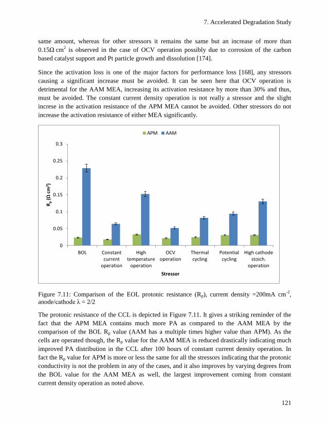
7. Accelerated Degradation Study
121
same amount, whereas for other stressors it remains the same but an increase of more than
0.15Ω cm2 is observed in the case of OCV operation possibly due to corrosion of the carbon
based catalyst support and Pt particle growth and dissolution [174].
Since the activation loss is one of the major factors for performance loss [168], any stressors
causing a significant increase must be avoided. It can be seen here that OCV operation is
detrimental for the AAM MEA, increasing its activation resistance by more than 30% and thus,
must be avoided. The constant current density operation is not really a stressor and the slight
increse in the activation resistance of the APM MEA cannot be avoided. Other stressors do not
increase the activation resistance of either MEA significantly.
Figure 7.11: Comparison of the EOL protonic resistance (Rp), current density =200mA cm-2
,
anode/cathode λ = 2/2
The protonic resistance of the CCL is depicted in Figure 7.11. It gives a striking reminder of the
fact that the APM MEA contains much more PA as compared to the AAM MEA by the
comparison of the BOL Rp value (AAM has a multiple times higher value than APM). As the
cells are operated though, the Rp value for the AAM MEA is reduced drastically indicating much
improved PA distribution in the CCL after 100 hours of constant current density operation. In
fact the Rp value for APM is more or less the same for all the stressors indicating that the protonic
conductivity is not the problem in any of the cases, and it also improves by varying degrees from
the BOL value for the AAM MEA as well, the largest improvement coming from constant
current density operation as noted above.
0
0.05
0.1
0.15
0.2
0.25
0.3
BOL Constantcurrent
operation
Hightemperature
operation
OCVoperation
Thermalcycling
Potentialcycling
High cathodestoich.
operation
Rp (
Ω c
m2 )
Stressor
APM AAM
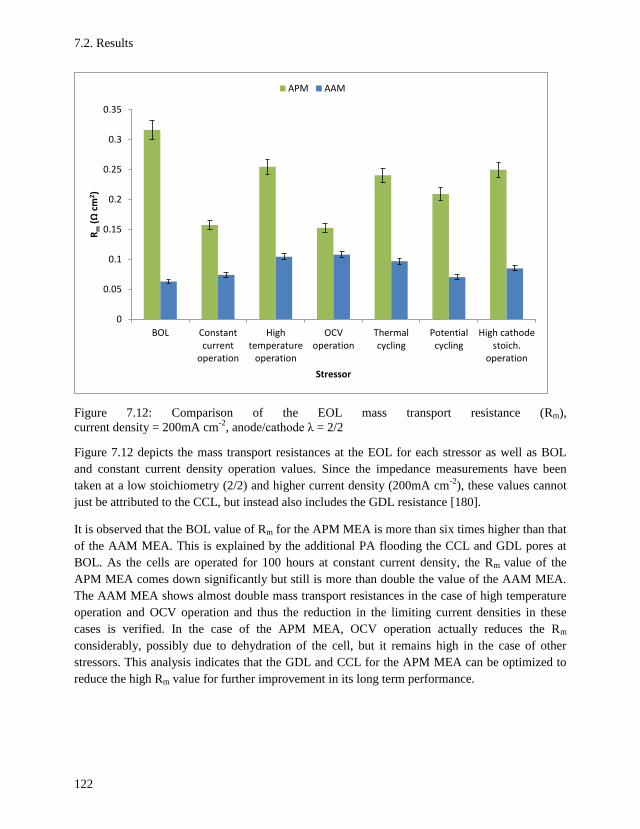
7.2. Results
122
Figure 7.12: Comparison of the EOL mass transport resistance (Rm),
current density = 200mA cm-2
, anode/cathode λ = 2/2
Figure 7.12 depicts the mass transport resistances at the EOL for each stressor as well as BOL
and constant current density operation values. Since the impedance measurements have been
taken at a low stoichiometry (2/2) and higher current density (200mA cm-2
), these values cannot
just be attributed to the CCL, but instead also includes the GDL resistance [180].
It is observed that the BOL value of Rm for the APM MEA is more than six times higher than that
of the AAM MEA. This is explained by the additional PA flooding the CCL and GDL pores at
BOL. As the cells are operated for 100 hours at constant current density, the Rm value of the
APM MEA comes down significantly but still is more than double the value of the AAM MEA.
The AAM MEA shows almost double mass transport resistances in the case of high temperature
operation and OCV operation and thus the reduction in the limiting current densities in these
cases is verified. In the case of the APM MEA, OCV operation actually reduces the Rm
considerably, possibly due to dehydration of the cell, but it remains high in the case of other
stressors. This analysis indicates that the GDL and CCL for the APM MEA can be optimized to
reduce the high Rm value for further improvement in its long term performance.
0
0.05
0.1
0.15
0.2
0.25
0.3
0.35
BOL Constantcurrent
operation
Hightemperature
operation
OCVoperation
Thermalcycling
Potentialcycling
High cathodestoich.
operation
Rm
(Ω
cm
2 )
Stressor
APM AAM
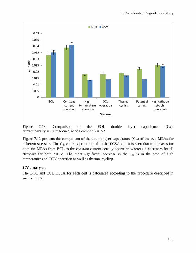
7. Accelerated Degradation Study
123
Figure 7.13: Comparison of the EOL double layer capacitance (Cdl),
current density = 200mA cm-2
, anode/cathode λ = 2/2
Figure 7.13 presents the comparison of the double layer capacitance (Cdl) of the two MEAs for
different stressors. The Cdl value is proportional to the ECSA and it is seen that it increases for
both the MEAs from BOL to the constant current density operation whereas it decreases for all
stressors for both MEAs. The most significant decrease in the Cdl is in the case of high
temperature and OCV operation as well as thermal cycling.
CV analysis
The BOL and EOL ECSA for each cell is calculated according to the procedure described in
section 3.3.2.
0
0.005
0.01
0.015
0.02
0.025
0.03
0.035
0.04
0.045
0.05
BOL Constantcurrent
operation
Hightemperature
operation
OCVoperation
Thermalcycling
Potentialcycling
High cathodestoich.
operation
Cd
l (F
cm-2
)
Stressor
APM AAM
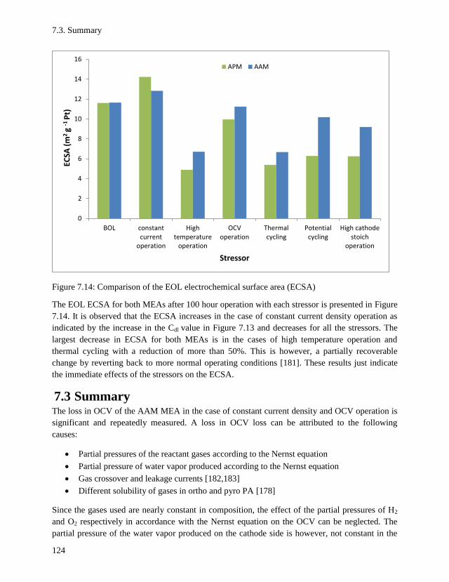
7.3. Summary
124
Figure 7.14: Comparison of the EOL electrochemical surface area (ECSA)
The EOL ECSA for both MEAs after 100 hour operation with each stressor is presented in Figure
7.14. It is observed that the ECSA increases in the case of constant current density operation as
indicated by the increase in the Cdl value in Figure 7.13 and decreases for all the stressors. The
largest decrease in ECSA for both MEAs is in the cases of high temperature operation and
thermal cycling with a reduction of more than 50%. This is however, a partially recoverable
change by reverting back to more normal operating conditions [181]. These results just indicate
the immediate effects of the stressors on the ECSA.
7.3 Summary The loss in OCV of the AAM MEA in the case of constant current density and OCV operation is
significant and repeatedly measured. A loss in OCV loss can be attributed to the following
causes:
Partial pressures of the reactant gases according to the Nernst equation
Partial pressure of water vapor produced according to the Nernst equation
Gas crossover and leakage currents [182,183]
Different solubility of gases in ortho and pyro PA [178]
Since the gases used are nearly constant in composition, the effect of the partial pressures of H2
and O2 respectively in accordance with the Nernst equation on the OCV can be neglected. The
partial pressure of the water vapor produced on the cathode side is however, not constant in the
0
2
4
6
8
10
12
14
16
BOL constantcurrent
operation
Hightemperature
operation
OCVoperation
Thermalcycling
Potentialcycling
High cathodestoich
operation
EC
SA (
m2
g -1
Pt)
Stressor
APM AAM
7. Accelerated Degradation Study
125
case of most stressors. This will not only have an influence in accordance to the Nernst equation,
but also it affects the PA hydration/dehydration processes which lead to variation of the PA
species concentration and PA distribution in the MEA and hence affects the fuel cell performance
as mentioned above due to the different protonic conductivity and solubility of gases in the two
PA species. Gas crossover and leakage currents can also affect the OCV and cell performance
according to the literature [84,184]. The APM MEA shows a very stable OCV behavior for all
the stressors with little change in the OCV.
Qi et al. [185] reported a mostly unrecoverable performance loss due to OCV operation of a HT-
PEFC. They associated this loss of performance to loss of catalytic activity, increased mass
transport resistance and increased Pt particle size by EIS and XRD measurements. In case of both
AAM and APM MEAs, significant loss of performance for just 100 hours of cell operation is
observed. The loss of ECSA in this case is not too large for either MEA, but the EOL mass
transport resistance is large for both MEAs possibly due to increased Pt particle size and a
resulting loss in catalytic activity as seen in the double layer capacitance comparison for OCV
operation.
Yu et al. [186] reported significant loss of PA as a major cause for degradation of HT-PEFCs at
higher temperatures (180oC or more). In the case of each MEA, high temperature operation and
thermal cycling are indeed very effective stressors and cause significant degradation at higher
current densities. This can be attributed to the loss of PA content. Since the AAM MEA has a
lower PA content, the observed degradation rates for high temperature operation and thermal
cycling for this MEA are much higher than for the APM MEA.
The effect of potential cycling on MEA performance is the least destructive in the case of both
MEAs. An increased EOL performance is observed in the case of the AAM MEA, whereas very
small degradation rates are observed for the APM MEA. There are contradicting reports in the
literature regarding the effect of potential cycling and reports of performance loss [58] and also
performance increase [177]. Further investigation is required to reach concrete conclusion about
the effects of potential cycling on HT-PEFC MEAs.
The effect of high cathode stoichiometry is radically different for the investigated MEAs. It is the
stressor with the most pronounced effect upto a current density of 550mA cm-2
(degradation rate
of 820µV h-1
) for the AAM MEA, whereas its effect is more than six times less for the APM
MEA at the same current density (degradation rate 132µV h-1
). This can be attributed to the loss
of PA (APM has much higher PA) as discussed previously and is a major degradation mechanism
for HT-PEFC operation [63].
This chapter has just scratched the surface of the degradation related issues for HT-PEFC. It is
hoped that it will inspire in depth and detailed analysis of the effects of different stressors on the
performance of the HT-PEFC and the associated degradation mechanisms which will ultimately
lead to a standardized AST for the HT-PEFC.

7.3. Summary
126
127
8 Discussion and Conclusions
The experimental work of this thesis can be broadly divided into two parts. The first part
concentrated on the determination of the best operating conditions and the degradation
mechanisms and rates for different stressors of the HT-PEFC MEAs in single cell operation.
Since material parameters and their effects on cell performance were not being directly
investigated in this part, commercially available HT-PEFC MEAs were used for these campaigns.
Chapters 4 and 7 covered this part. The second part concerned analyzing the material parameters
of the in-house assembled HT-PEFC MEA and determining the underlying physical phenomena
causing different cell performance. Possible improvements were also suggested by utilizing both
the DoE and the EIS methods. Chapters 5 and 6 addressed this issue. The overall discussion of
the results is presented in the next section.
8.1 Discussion The DoE has been used in various research areas related to fuel cell technology and is gaining
popularity due to its obvious advantages regarding resources, experimental planning and
incorporation of factor interactions. Al-Hadeethi et al. [187] used the response surface
methodology to determine the effect of temperature, gas flowrate and different flow
configurations (co and counter-flow) on the performance of a LT- PEFC. This is interesting in the
fact that a qualitative variable (flow configuration) is included in the analysis. Usually, inclusion
of such a variable sways the planners towards OFAT, but the authors used the DoE successfully
and determined a strong interaction between the temperature and flowrate of gases for the
investigated range. They used the regression models to predict the cell performance very
accurately. Other examples of successful DoE application in fuel cell research can be seen in
[104–107,188–190].
The impact of four important operating conditions (current density, operating temperature, and
anode and cathode stoichiometries) on the performance of four commercial MEAs was
investigated using a full factorial DoE in chapter 4. The main effects and interactions of the
factors were determined to build statistical models for predicting cell voltages in the range of
investigation of each factor. A comparison of the two sample sizes used (5 and 30) revealed the
reliability of the statistical models based on a smaller sample size for a screening design. This
indicates potential for significant savings in resources (costs, time and human resources) without
compromising on the accuracy of results. It was determined that current density, operating
temperature and their interaction were statistically significant for all the tested MEAs and hence
featured in the corresponding statistical models. Taking UI curves at different factor setting
allowed construction of reliable statistical models for different current densities while eliminating
the current density explicitly from the models. These UI curves were named “DoE UI curves”
and add a new dimension to MEA testing in single cells. It was also observed that the MEAs
Celtec®
PW1100 and DPS showed performance improvement and little or no degradation at the
8.1. Discussion
128
EOL whereas the other two MEAs tested showed some degradation. Although, the impact of the
four investigated factors on HT-PEFC has been previously published in the literature [75,191–
193], these are mostly stack based studies with different goals and therefore no direct
comparisons of screening designs of HT-PEFC MEAs are available in the literature. However, it
is hoped that the methodology presented in this thesis will become the norm for screening designs
in the future.
The Celtec®
PW1100 MEA (previously manufactured by BASF) materials and manufacturing
processes have been recently acquired by Advent Technologies®
and the same MEA is now
available under the product series APM from Advent Technologies®
. This MEA, along with
another HT-PEFC MEA (AAM) with a TPS membrane and a carbon cloth based GDL material,
also from Advent technologies®
were selected for the degradation testing campaign (Chapter 7).
The degradation testing showed a significant amount of degradation in both the MEAs with only
100 hour operation under the selected stressors. However, both MEAs showed performance
improvement (in excess of 200µV h-1
at 600mA cm-2
) for 100 hours of constant current density
(200mA cm-2
) operation. The trend for performance improvement is even higher for higher
current densities implying reduced mass transport losses due to increased diffusion of the reactant
gases to the TPB sites and improved PA distribution in the MEA. This would suggest considering
increasing the currently standard break-in procedure time from 72 hours to 100 hours to
maximize the constant current density operation at BOL of the cell, since it seems to optimize the
PA redistribution in the MEA and improve the cell performance. Rabjerg [194] concluded the
opposite for both sol-gel and post doped (doped after casting) HT-PEFC MEAs and suggested
reducing the break-in duration for both types. This, however, contradicts our observations as
discussed above.
The trends of the actual stressors on the MEA performance were much different for the AAM and
APM MEAs. This has to do with the different membranes (PBI based for APM and TPS for
AAM) as well as the different PA content (much higher in APM) and the doping procedures (sol-
gel for APM and post doping for AAM MEA) of the MEAs. Also, both MEAs use carbon cloth
as the porous material for the GDE, albeit, different carbon cloth materials [127] and the catalyst
layers have similar Pt loadings. High cathode stoichiometry and thermal cycling caused the
greatest degradation rates for the AAM MEA with a linear increase in the degradation rates with
current density. The degradation rate caused by constant high temperature operation and OCV
operation was also linear upto a current density of 450mA cm-2
, but the AAM MEA showed an
exponential increase in the degradation rates at higher current densities signifying a much
reduced limiting current density for the AAM MEA after 100 hour OCV operation, presumably
due to loss of catalytic activity, increased concentration resistance and increased size of Pt
particles. Since the measured ECSA shows less than 10% decrease from BOL, the exponential
increase in the degradation rates at higher current densities can be attributed mainly to the
increased concentration resistance and Pt particle sizes. The Pt particle sizes could not be
examined in this case, since it is not allowed to do post mortem analysis of the commercial HT-
PEFC MEAs due to non-disclosure agreements (NDA) with the MEA suppliers; however the
8. Discussion and Conclusions
129
EOL concentration resistance as calculated by the EIS data indicated almost 100% increase from
the BOL value, thus supporting the above argument. The increase in Pt particle size is also well
documented in the literature with Qi et al. [185] reporting a Pt particle size increase of as much as
430% with OCV operation of 244.5 hours of a PBI based HT-PEFC MEA. De beer et al. [63]
operated a HT-PEFC for 24 hours at OCV conditions without any flow of gases on either side
and measured a substantially worse polarization curve and higher low frequency resistance in the
Nyquist plot. They attributed these changes mainly to carbon corrosion of the catalyst support as
well as in the GDL. The OCV operation in this study however, is different in that the flow of the
gases was not completely shut off, but held constant for the values of anode/cathode
stoichiometry of 2/2 at a current density of 200mA cm-2
. This resulted in a smaller decrease in the
ECSA. Oono et al. [195] operated HT-PEFC single cells for about 18,000 hours at constant
current density (200mA cm-2
) and attributed the steady decrease in cell performance during the
first 14,000 hours to Pt agglomeration and the later more pronounced degradation to the
membrane thinning and migration into the CL with the PA.
Load cycling for 100 hours actually improved cell performance for the AAM MEA and caused
insignificant degradation in the case of the APM MEA. Due to the scarce and contradicting
reports in the literature with regard to effect of load cycling on HT-PEFC performance, with
some reporting a performance loss and some reporting an improvement, it was concluded that
100 hour operation is not enough to come to any concrete conclusions about the effects and
causes of load cycling on the tested MEAs. The actual structure of the cycle used also has a
profound effect. The cycle used in this study uses current density steps of 0.05A cm-2
with time
steps of 5 minutes in the range of 0.2 to 0.6A cm-2
. This implementation mode seems to be
favorable for both MEAs. Other cycles used in the literature usually have smaller time steps
combined with larger current density steps resulting in different degradation rates. Thomas et al.
[177] cycled four HT-PEFC single cells under load cycling between current densities of 200 and
800mA cm-2
and compared the degradation rates with a cell that was operated at a constant
current density of 200mA cm-2
to find that load cycles which spent higher time at the lower
current density actually had 1.5 times less degradation than the cell operated continuously at
constant current density. They used rest times (operation time at the lower current density, the
cells were operated at the higher current density for the rest of the time) from 15 seconds to 2
minutes and that the cell with the highest rest time showed the least degradation in a total
operation time of about 2000 hours. Jeon et al. [196] found much more degradation of the cycled
cells in comparison to the reference cell which was operated at a constant voltage of 0.6V. The
cycles also used very small time steps (500 cycles in 35 hours) and different voltage ranges upto
1V. Rastedt et al. [197] used 6 minutes at 0.6A cm-2
and 14 minutes at 1A cm-2
as their load
cycling protocol. They tested four different HT-PEFC MEAs with varied degradation. This
discussion can be concluded by reasserting the need of a harmonized protocol for load cycling
among the fuel cell industry to have more comparable results.
The degradation of the APM MEA had a different pattern altogether, with high temperature
operation, OCV operation and thermal cycling causing the highest degradation rates. The
8.1. Discussion
130
degradation rates for constant high temperature operation for current densities higher than
500mA cm-2
were quadratic indicating an increased concentration resistance. This can be
attributed to the considerable loss of PA, since the APM MEA has a high PA content and at high
temperature operation (T > 180oC), significant PA loss has been reported to be a dominant
degradation mode for HT-PEFC MEAs [186]. The degradation rates for the AAM MEA were
also very high for high temperature operation and thermal cycling, reinforcing this fact. High
cathode stoichiometry, which causes drying out of the cell and a change in the PA species
concentration in the MEA, did not cause a very high degradation for the APM MEA as for the
AAM MEA, signifying the presence of additional PA for the APM MEA leading to a lesser
dehydration effect. Søndergaard et al. [85] attributed the total amount of gas volume passed
through a HT-PEFC during its lifetime, as well as other operating conditions such as current
density and operating temperature to the rate of acid loss. They operated their cells in the range of
2 to 25 gas stoichiometries, 200 to 800mA cm-2
current density and 160 to 180oC operating
temperatures. This study also used comparable conditions, although the high cathode
stoichiometry used was 12. PA loss contributed significantly in most cases as discussed in section
7.3 to the observed degradation of the MEAs. Oono et al. [198] determined Pt agglomeration to
be temperature dependent in early degradation, but found no effect of temperature on the
depletion of PA rate, which caused a much higher degradation in the terminal stages of a long
term test conducted on three HT-PEFC MEAs at cell temperatures of 150, 170 and 190oC
respectively. They also found the least degradation in the cell operating at the lowest temperature.
The impedance analysis of both MEAs after 100 hour of stressor operation showed that RΩ and
Rp significantly increased for the AAM MEA while remaining more or less constant for the APM
MEA. The Rm value was the limiting factor for the APM MEA, increasing significantly from the
constant current density value for each stressor. The CV analysis showed a loss of ECSA for
most of the stressors for both MEAs, but its recoverability was not quantified by reverting back to
normal operating conditions for a substantial amount of time in this study. The main differences
in the degradation behavior of the two investigated MEAs can also be attributed to the different
materials (GDEs) and doping procedures (sol-gel vs. post doping after casting) to a certain extent
[199], however, the separation and quantification of these effects was not a part of this study.
The second part of this experimental study concentrated on the improvement of the in-house
assembled HT-PEFC MEA (Chapters 5 and 6). The idea was to characterize the performance of
the CCL as it is the performance limiting part of the MEA (for pure hydrogen operation). Chapter
5 considered three major material parameters for the MEA and evaluated their combined effect
on the single cell performance by using the DoE method for three different current densities (200,
400 and 600mA cm-2
). The considered factors were CCL thickness, PADL of the MEA and Pt
loading of the CCL. Analysis of the results indicated significant interactions between the factors
and the response surface indicated maximum cell performance with a CCL thickness of 120µm, a
PADL of 15mg cm-2
and a CCL Pt loading of 1mg cm-2
. A Pt loading of 0.6mg cm-2
also showed
promising results, but the factor interactions favor the higher Pt loading value. An impedance
analysis of the CCL electrochemical parameters indicated that the MEA with the suggested
8. Discussion and Conclusions
131
material parameters of 120µm CCL thickness, 15mg cm-2
PADL and 1mg cm-2
Pt loading had a
much lower Ract in the low current and high stoichiometry regime than the other MEAs. Since
Ract dominates the Tafel region, this MEA was determined to be the better one in comparison
with the MEA with same CCL thickness and PADL, but a lower Pt loading of 0.6mg cm-2
also
showing promising performance. The improvement area for the selected MEA was the Rp, which
was almost double than the other MEAs (0.175Ω cm2 compared to values close to 0.1Ω cm
2 for
the other MEAs) and must be improved for better cell performance at higher current densities.
The PADL is a very important material parameter for HT-PEFC MEA performance. Oono et al.
[200] investigated different doping levels for HT-PEFC single cells and concluded that a doping
level of 10mg cm-2
is optimum for a CL thickness of 20µm and a Pt loading of 0.7mg cm-2
. The
present study would seem to contradict this result as the CCL thickness is 3 to 6 times higher (60
and 120µm) and yet an increase in the doping level above 15mg cm-2
causes a decrease in cell
performance with the main effect of Pt loading being insignificant but a strong interaction
between Pt loading and the CCL thickness. The PA doping process is also similar to the one used
by Oono et al. (post doping after casting the membrane). They immersed the PBI membranes (no
details provided) in 85% PA solution for a calculated amount of time (determined by an ex-situ
survey) at 20, 40 and 60oC. The AM-55 membrane by FUMA-Tech was also doped by
immersing it in 85% PA solution, but the temperature used was 110oC and the immersion time
was 2 hours. The GDL material used was also different (TGP-H-090 Toray paper). Also, the
catalyst ink recipe was different. Although, the two studies are not directly comparable, lessons
can be learnt from this study, as a thinner CCL is highly desirable (reduced losses across the
CCL) if it can withstand a higher PADL. The Pt loading of a HT-PEFC is generally in the range
of 1mg cm-2
or even higher for commercial MEAs [127,128,201,202]. This is much higher than
the Pt loading of the LT-PEFC electrodes which are currently in the range of 0.1 to 0.4mg cm-2
[203] with intense ongoing research for further reduction. The research in this regard in the field
of HT-PEFC also needs to be increased. Liang et al. [126] achieved cathode loadings as low as
0.3mg cm-2
by using the CCM method for manufacturing the HT-PEFC MEA and Su et al. [142]
reported achieving a peak power density of 0.339W cm-2
and peak cathode mass power of
0.967W mg-1
Pt with a cathode loading of 0.350mg cm-2
. Martin et al. [72] achieved a peak
power density of 0.482W cm-2
with oxygen and 0.321W cm-2
with air on the cathode side with
PBI based membranes using no binder material in the CCL and Pt loading of 0.1mg cm-2
. They
attributed this to the extended TPB in the CCL due to avoidance of the PA flooding of the CCL.
These results are encouraging, but still laboratory based and a higher Pt loading remains the norm
for HT-PEFC for now until long term stability and acceptable degradation rates can be achieved
in addition to high performance. Unfortunately, not much experimental work has been done on
optimizing the CCL thickness in HT-PEFC MEAs, and further research needs to be done in this
area to determine the optimum balance between these three critical CCL material parameters.
Chapter 6 investigated the effect of varying anode and cathode gas composition on cell
impedance in the high stoichiometry and low current density regime. The impedance data was
analyzed with an ECM and also an analytical model by Kulikovsky valid for the low current
density regime and the results were compared. An improved ECM was suggested on the basis of
8.2. Conclusions
132
the comparison, which would use two parallel RC combinations in the low current density
regime, where the second RC combination can be used to calculate the oxygen transport
limitation in the CCL. Although there are many reports of ECM based, numerical and analytical
modelling of PEFC impedance in the literature [80–83,116,121–
123,147,157,160,166,167,180,204–218], the novelty of the present work lies in the comparison
with an ECM and extraction of means to determine relevant physical parameters to the CCL in
the HT-PEFC MEA by improving the ECM.
The issues regarding HT-PEFC operation, performance and degradation investigated in this thesis
represent some of the main obstacles to its commercialization. If addressed, the HT-PEFC has the
potential to serve the energy sector, especially in transport and CHP applications, in the transition
period to a completely hydrogen based sustainable economy.
8.2 Conclusions This thesis concentrated on analyzing and quantifying the effects of different operating
conditions and material parameters on the performance of the HT-PEFC MEA at the single cell
level. The DoE methodology was used extensively to determine statistical models and response
surfaces for the factors being considered. EIS was used for the quantification and comparison of
the characteristic electrochemical parameters of the fuel cell and compare them to determine the
most desirable conditions/parameters for MEA performance improvement. The main conclusions
of this work are presented below.
A small sample size (n=5) can be used for a full factorial DoE for screening MEA
designs.
PA loss, loss of Pt surface area by particle size growth, migration, agglomeration and
dissolution, and carbon corrosion are three of the main degradation mechanisms
responsible for performance loss in HT-PEFC operation with pure hydrogen.
An in-house assembled MEA with a CCL thickness of 120µm, PADL of 15mg cm-2
and
cathode Pt loading of 1mg cm-2
is recommended as the most suitable from a performance
viewpoint with further suggestions for improvement.
A novel interpretation of a classical ECM is suggested in the low current density and high
stoichiometry regime, for the approximation of mass transport resistance of the CCL from
EIS data.
133
Nomenclature
Abbreviations
AFC alkaline fuel cell
AM analytical model
AST accelerated stress test
BOL beginning of life
CCL cathode catalyst layer
CE counter electrode
CL catalyst layer
CPE constant phase element
CV cyclic voltammetry
DMFC direct methanol fuel cell
DoE design of experiments (method)
ECM equivalent circuit model
ECSA electro chemical surface area
EIS electrochemical impedance spectroscopy
EOL end of life
FRA frequency response analyzer
GDE gas diffusion electrode
GDL gas diffusion layer
GHG greenhouse gases
HHV higher heating value
HOR hydrogen oxidation reaction
HT-PEFC high temperature polymer electrolyte fuel cell
ICE internal combustion engine
Nomenclature
134
LHV lower heating value
LT-PEFC low temperature polymer electrolyte fuel cell
MCFC molten carbonate fuel cell
MEA membrane electrode assembly
MPL micro porous layer
OCV open circuit voltage
OFAT one factor at a time (method)
ORR oxygen reduction reaction
PA phosphoric acid
PADL phosphoric acid doping level
PAFC phosphoric acid fuel cell
PBI polybenzimidazole
PFA perfluoroalkoxy
PEFC polymer electrolyte fuel cell
PTFE polytetrafluoroethylene
SOFC solid oxide fuel cell
SS stainless steel
STP standard temperature pressure
TPB triple phase boundary
WE working electrode

Nomenclature
135
Latin Symbols
b mV per decade Tafel slope
C Farad capacitance
Cdl Farad cm-2
double layer capacitance
Cdl Farad cm-3
volumetric double layer capacitance
Cref mol cm-3
reference oxygen concentration
Db cm2 s
-1 diffusion constant of oxygen in the GDL
Doxp cm2 s
-1 diffusion constant of oxygen in the CCL
E V Nernst fuel cell potential
Ecell V fuel cell voltage
ECSA m² g-1
electrochemically active Pt surface area
Eo V theoretical fuel cell potential
f Hz frequency
fi individual frequency (of effects)
F 96485C mol-1
Faraday’s constant
i A current
j imaginary number prefix
jo A cm-2
current density
k number of factor to be analyzed
L Henry Inductance
lt cm CCL thickness
P atm pressure
P probability of the occurrence of an event
PH2 normalized partial pressure of hydrogen
Po atm atmospheric pressure

Nomenclature
136
PO2 normalized partial pressure of oxygen
PH2O normalized partial pressure of water vapor
Q C cm-2
charge per unit area/ pre-factor of a CPE
n exponent of a CPE
n number of samples
n number of experiments required
n total number of effects
n number of electrons per molecule of hydrogen
R Ω resistance
Ract Ω cm2
activation resistance
Rdc Ω cm2
DC resistance
RΩ Ω cm2
ohmic resistance
Rp Ω cm2
protonic resistance
Rm Ω cm2
mass transport resistance
Roxp Ω cm2
mass transport resistance of the CCL
T K absolute temperature
V V voltage
Z Ω cm2 impedance
Zi Ω cm2
Z score of the ith effect
ZCPE Ω cm2 impedance of the CPE
Greek Symbols
ΔG kJ mol-1 change in Gibbs free energy of the reaction
ΔH kJ mol-1 enthalpy change of the reaction
ΔS kJ mol-1
K-1 entropy change of the reaction
ηact V activation overpotential
Nomenclature
137
ηconc V concentration overpotential
ηmax maximum efficiency
ηohm V ohmic overpotential
λ stoichiometric ratio
Φ degrees phase angle
σp S cm-1
protonic conductivity
Ɛ experimental error
ω rad s-1
angular frequency
138
Bibliography [1] Marbán G, Valdés-Solís T. Towards the hydrogen economy? International Journal of
Hydrogen Energy 2007;32:1625–37. doi:10.1016/j.ijhydene.2006.12.017.
[2] Graves PE. Implications of global warming: Two eras. World Development Perspectives
2017;7–8:9–14. doi:10.1016/j.wdp.2017.10.002.
[3] Shukla JB, Verma M, Misra AK. Effect of global warming on sea level rise: A modeling
study. Ecological Complexity 2017;32:99–110. doi:10.1016/j.ecocom.2017.10.007.
[4] Bong CPC, Lim LY, Ho WS, Lim JS, Klemeš JJ, Towprayoon S, et al. A review on the
global warming potential of cleaner composting and mitigation strategies. Journal of
Cleaner Production 2017;146:149–57. doi:10.1016/j.jclepro.2016.07.066.
[5] Jain IP. Hydrogen the fuel for 21st century. International Journal of Hydrogen Energy
2009;34:7368–78. doi:10.1016/j.ijhydene.2009.05.093.
[6] Barreto L, Makihira A, Riahi K. The hydrogen economy in the 21st century: A sustainable
development scenario. International Journal of Hydrogen Energy 2003;28:267–84.
doi:10.1016/S0360-3199(02)00074-5.
[7] Crabtree GW, Dresselhaus MS, Buchanan M V. The Hydrogen Economy. Physics Today
2004:39–45. doi:10.1063/1.1878333.
[8] Barbir F. Introduction. PEM Fuel Cells, Elsevier; 2013, p. 1–16. doi:10.1016/B978-0-12-
387710-9.00001-1.
[9] Wang Y, Chen KS, Mishler J, Cho SC, Adroher XC. A review of polymer electrolyte
membrane fuel cells: Technology, applications, and needs on fundamental research.
Applied Energy 2011;88:981–1007. doi:10.1016/j.apenergy.2010.09.030.
[10] Donitz W. Fuel cells for mobile applications, status, requirements and future application
potential. International Journal of Hydrogen Energy 1998;23:611–5. doi:10.1016/S0360-
3199(97)00075-X.
[11] P.Corbo, Migliardini.F, Veneri.O. Hydrogen Fuel Cells for Road Vehicles. Springer; 2011.
doi:10.1007/978-0-85729-136-3.
[12] Chalk SG, Miller JF, Wagner FW. Challenges for fuel cells in transport applications.
Journal of Power Sources 2000;86:40–51. doi:10.1016/S0378-7753(99)00481-4.
[13] Barbir F. Fuel Cell Electrochemistry. PEM Fuel Cells, Elsevier; 2013, p. 33–72.
doi:10.1016/B978-0-12-387710-9.00003-5.
[14] O’hayre R, Cha S-W, Colella WG, Prinz FB. Fuel Cell Technology. Fuel Cell
Fundamentals. 3rd ed., Wiley; 2016.
[15] Park S, Lee J-W, Popov BN. A review of gas diffusion layer in PEM fuel cells: Materials
and designs. International Journal of Hydrogen Energy 2012;37:5850–65.
doi:10.1016/j.ijhydene.2011.12.148.
Bibliography
139
[16] Park J, Oh H, Ha T, Lee Y Il, Min K. A review of the gas diffusion layer in proton
exchange membrane fuel cells: Durability and degradation. Applied Energy
2015;155:866–80. doi:10.1016/j.apenergy.2015.06.068.
[17] Ye DH, Zhan ZG. A review on the sealing structures of membrane electrode assembly of
proton exchange membrane fuel cells. Journal of Power Sources 2013;231:285–92.
doi:10.1016/j.jpowsour.2013.01.009.
[18] Song J, De castro S, Yu S. BASF Stack Handbook. 2011.
[19] Middelman E, Kout W, Vogelaar B, Lenssen J, de Waal E. Bipolar plates for PEM fuel
cells. Journal of Power Sources 2003;118:44–6. doi:10.1016/S0378-7753(03)00070-3.
[20] Jung S-P, Lee C-I, Chen C-C, Chang W-S, Yang C-C. Development of novel proton
exchange membrane fuel cells using stamped metallic bipolar plates. Journal of Power
Sources 2015;283:429–42. doi:10.1016/j.jpowsour.2015.02.145.
[21] Wang Y, Northwood DO. An investigation into polypyrrole-coated 316L stainless steel as
a bipolar plate material for PEM fuel cells. Journal of Power Sources 2006;163:500–8.
doi:10.1016/j.jpowsour.2006.09.048.
[22] Zaidi SMJ, Matsuura T. Polymer Membranes for Fuel Cells. springer; 2009.
doi:10.1007/978-0-387-73532-0.
[23] Kulikovsky A, Eikerling M. Basic Concepts. Polymer Electrolyte Fuel Cells :Physical
principles of materials and operation, CRC Press Taylor & Francis Group; 2015, p. 1–28.
[24] Kandlikar SG, Lu Z. Thermal management issues in a PEMFC stack – A brief review of
current status. Applied Thermal Engineering 2009;29:1276–80.
doi:10.1016/j.applthermaleng.2008.05.009.
[25] Li H, Tang Y, Wang Z, Shi Z, Wu S, Song D, et al. A review of water flooding issues in
the proton exchange membrane fuel cell. Journal of Power Sources 2008;178:103–17.
doi:10.1016/j.jpowsour.2007.12.068.
[26] Dai W, Wang H, Yuan X-Z, Martin JJ, Yang D, Qiao J, et al. A review on water balance in
the membrane electrode assembly of proton exchange membrane fuel cells. International
Journal of Hydrogen Energy 2009;34:9461–78. doi:10.1016/j.ijhydene.2009.09.017.
[27] Ji M, Wei Z. A review of water management in polymer electrolyte membrane fuel cells.
Energies 2009;2:1057–106.
[28] Sui S, Wang X, Zhou X, Su Y, Riffat S, Liu C. A comprehensive review of Pt
electrocatalysts for the oxygen reduction reaction: Nanostructure, activity, mechanism and
carbon support in PEM fuel cells. J Mater Chem A 2017;5:1808–25.
doi:10.1039/C6TA08580F.
[29] Shao M, Chang Q, Dodelet J-P, Chenitz R. Recent Advances in Electrocatalysts for
Oxygen Reduction Reaction. Chemical Reviews 2016;116:3594–657.
doi:10.1021/acs.chemrev.5b00462.
[30] Stacy J, Regmi YN, Leonard B, Fan M. The recent progress and future of oxygen
Bibliography
140
reduction reaction catalysis: A review. Renewable and Sustainable Energy Reviews
2017;69:401–14. doi:10.1016/j.rser.2016.09.135.
[31] Changlin Zhang, Yanbo Pan, Zhenmeng Peng XS. A review of Pt-based electrocatalysts
for oxygen reduction reaction. Frontiers in Energy n.d.;11:268–85.
[32] Araya SS, Zhou F, Liso V, Sahlin SL, Vang JR, Thomas S, et al. A comprehensive review
of PBI-based high temperature PEM fuel cells. International Journal of Hydrogen Energy
2016;41:21310–44. doi:10.1016/j.ijhydene.2016.09.024.
[33] Rosli RE, Sulong AB, Daud WR, Zulkifley MA, Husaini T, Rosli MI, et al. A review of
high-temperature proton exchange membrane fuel cell (HT-PEMFC) system. International
Journal of Hydrogen Energy 2017;42:9293–314. doi:10.1016/j.ijhydene.2016.06.211.
[34] Authayanun S, Im-orb K, Arpornwichanop A. A review of the development of high
temperature proton exchange membrane fuel cells. Chinese Journal of Catalysis
2015;36:473–83. doi:10.1016/S1872-2067(14)60272-2.
[35] Chandan A, Hattenberger M, El-kharouf A, Du S, Dhir A, Self V, et al. High temperature
(HT) polymer electrolyte membrane fuel cells (PEMFC) – A review. Journal of Power
Sources 2013;231:264–78. doi:10.1016/j.jpowsour.2012.11.126.
[36] Li Q, Jensen JO, Savinell RF, Bjerrum NJ. High temperature proton exchange membranes
based on polybenzimidazoles for fuel cells. Progress in Polymer Science 2009;34:449–77.
doi:10.1016/j.progpolymsci.2008.12.003.
[37] Haque MA, Sulong ABB, Loh KSS, Majlan EH, Husaini T, Rosli RE. Acid doped
polybenzimidazoles based membrane electrode assembly for high temperature proton
exchange membrane fuel cell: A review. International Journal of Hydrogen Energy
2016;42:9156–79. doi:10.1016/j.ijhydene.2016.03.086.
[38] Cheng X, Shi Z, Glass N, Zhang L, Zhang J, Song D, et al. A review of PEM hydrogen
fuel cell contamination: Impacts, mechanisms, and mitigation. Journal of Power Sources
2007;165:739–56. doi:10.1016/j.jpowsour.2006.12.012.
[39] G. Qian and B. C. Benicewicz. Fuel Impurity Effects on High Temperature PBI Based
Fuel Cell Membranes. Transactions, E C S Society, The Electrochemical 2011;41:1441–8.
[40] Das SK, Reis A, Berry KJ. Experimental evaluation of CO poisoning on the performance
of a high temperature proton exchange membrane fuel cell. Journal of Power Sources
2009;193:691–8. doi:10.1016/j.jpowsour.2009.04.021.
[41] Zhang C, Zhou W, Ehteshami MM, Wang Y, Chan SH. Determination of the optimal
operating temperature range for high temperature PEM fuel cell considering its
performance, CO tolerance and degradation. Energy Conversion and Management
2015;105:433–41. doi:10.1016/j.enconman.2015.08.011.
[42] Krishnan P, Park J-S, Kim C-S. Performance of a poly(2,5-benzimidazole) membrane
based high temperature PEM fuel cell in the presence of carbon monoxide. Journal of
Power Sources 2006;159:817–23. doi:10.1016/j.jpowsour.2005.11.071.
Bibliography
141
[43] Samsun RC, Pasel J, Janßen H, Lehnert W, Peters R, Stolten D. Design and test of a 5kWe
high-temperature polymer electrolyte fuel cell system operated with diesel and kerosene.
Applied Energy 2014;114:238–49. doi:10.1016/j.apenergy.2013.09.054.
[44] Pan C, He R, Li Q, Jensen JO, Bjerrum NJ, Hjulmand HA, et al. Integration of high
temperature PEM fuel cells with a methanol reformer. Journal of Power Sources
2005;145:392–8. doi:10.1016/j.jpowsour.2005.02.056.
[45] Farrell CG, Gardner CL, Ternan M. Experimental and modelling studies of CO poisoning
in PEM fuel cells. Journal of Power Sources 2007;171:282–93.
doi:10.1016/j.jpowsour.2007.07.006.
[46] Liu Y, Lehnert W, Janßen H, Samsun RC, Stolten D. A review of high-temperature
polymer electrolyte membrane fuel-cell (HT-PEMFC)-based auxiliary power units for
diesel-powered road vehicles. Journal of Power Sources 2016;311:91–102.
doi:10.1016/j.jpowsour.2016.02.033.
[47] Zhu Y, Zhu WH, Tatarchuk BJ. Performance comparison between high temperature and
traditional proton exchange membrane fuel cell stacks using electrochemical impedance
spectroscopy. Journal of Power Sources 2014;256:250–7.
doi:10.1016/j.jpowsour.2014.01.049.
[48] Authayanun S, Mamlouk M, Scott K, Arpornwichanop A. Comparison of high-
temperature and low-temperature polymer electrolyte membrane fuel cell systems with
glycerol reforming process for stationary applications. Applied Energy 2013;109:192–201.
doi:10.1016/j.apenergy.2013.04.009.
[49] Maximini M, Engelhardt P, Brenner M, Beckmann F, Moritz O. Fast start-up of a diesel
fuel processor for PEM fuel cells. International Journal of Hydrogen Energy
2014;39:18154–63. doi:10.1016/j.ijhydene.2014.02.168.
[50] Wang Y, Sauer DU, Koehne S, Ersoez A. Dynamic modeling of high temperature PEM
fuel cell start-up process. International Journal of Hydrogen Energy 2014;39:19067–78.
doi:10.1016/j.ijhydene.2014.09.095.
[51] Jeong YH, Oh K, Ahn S, Kim NY, Byeon A, Park HY, et al. Investigation of electrolyte
leaching in the performance degradation of phosphoric acid-doped polybenzimidazole
membrane-based high temperature fuel cells. Journal of Power Sources 2017;363:365–74.
doi:10.1016/j.jpowsour.2017.07.109.
[52] Mack F, Heissler S, Laukenmann R, Zeis R. Phosphoric acid distribution and its impact on
the performance of polybenzimidazole membranes. Journal of Power Sources
2014;270:627–33. doi:10.1016/j.jpowsour.2014.06.171.
[53] Reimer U, Ehlert J, Janßen H, Lehnert W. Water distribution in high temperature polymer
electrolyte fuel cells. International Journal of Hydrogen Energy 2016;41:1837–45.
doi:10.1016/j.ijhydene.2015.11.106.
[54] Bevilacqua N, George MG, Galbiati S, Bazylak A, Zeis R. Phosphoric Acid Invasion in
High Temperature PEM Fuel Cell Gas Diffusion Layers. Electrochimica Acta
2017;257:89–98. doi:10.1016/j.electacta.2017.10.054.
Bibliography
142
[55] Modestov AD, Tarasevich MR, Filimonov VY, Zagudaeva NM. Degradation of high
temperature MEA with PBI-H3PO4membrane in a life test. Electrochimica Acta
2009;54:7121–7. doi:10.1016/j.electacta.2009.07.031.
[56] Mamlouk M, Scott K. Analysis of high temperature polymer electrolyte membrane fuel
cell electrodes using electrochemical impedance spectroscopy. Electrochimica Acta
2011;56:5493–512. doi:10.1016/j.electacta.2011.03.056.
[57] Dhanushkodi SR, Kundu S, Fowler MW, Pritzker MD. Study of the effect of temperature
on Pt dissolution in polymer electrolyte membrane fuel cells via accelerated stress tests.
Journal of Power Sources 2014;245:1035–45. doi:10.1016/j.jpowsour.2013.07.016.
[58] Yasuda K, Taniguchi A, Akita T, Ioroi T, Siroma Z. Platinum dissolution and deposition in
the polymer electrolyte membrane of a PEM fuel cell as studied by potential cycling. Phys
Chem Chem Phys 2006;8:746–52. doi:10.1039/B514342J.
[59] Mitsuda K, Murahashi T, Matsumoto M, Usami K. Estimation of corrosion conditions of a
phosphoric acid fuel cell. Journal of Applied Electrochemistry 1993;23:19–25.
doi:10.1007/BF00241570.
[60] Mitsuda K, Murahashi T. Air and fuel starvation of phosphoric acid fuel cells: A study
using a single cell with multi-reference electrodes. Journal of Applied Electrochemistry
1991;21:524–30. doi:10.1007/BF01018605.
[61] Reimer U, Schumacher B, Lehnert W. Accelerated Degradation of High-Temperature
Polymer Electrolyte Fuel Cells: Discussion and Empirical Modeling. Journal of the
Electrochemical Society 2014;162:F153–64. doi:10.1149/2.0961501jes.
[62] Schmittinger W, Vahidi A. A review of the main parameters influencing long-term
performance and durability of PEM fuel cells. Journal of Power Sources 2008;180:1–14.
doi:10.1016/j.jpowsour.2008.01.070.
[63] de Beer C, Barendse P, Pillay P, Bullecks B, Rengaswamy R. Classification of High
Temperature PEM Fuel Cell Degradation Mechanisms Using Equivalent Circuits. IEEE
Transactions on Industrial Electronics 2015;62. doi:10.1109/TIE.2015.2393292.
[64] Liu G, Zhang H, Hu J, Zhai Y, Xu D, Shao Z gang. Studies of performance degradation of
a high temperature PEMFC based on H3PO4-doped PBI. Journal of Power Sources
2006;162:547–52. doi:10.1016/j.jpowsour.2006.07.008.
[65] Zhang J, Xie Z, Zhang J, Tang Y, Song C, Navessin T, et al. High temperature PEM fuel
cells. Journal of Power Sources 2006;160:872–91. doi:10.1016/j.jpowsour.2006.05.034.
[66] Luan Y, Zhang Y. Membrane Degradation. In: Wang H, editor. PEM Fuel Cell Failure
Mode Analysis, CRC Press Taylor & Francis Group; 2012, p. 73–102.
[67] Lehnert W, Wannek C, Zeis R. High Temperature Polymer Electrolyte Fuel Cells. In:
Steinberger-Wilckens R, Lehnert W, editors. Innovations in Fuel Cell Technologies,
Cambridge: Royal Society of Chemistry; 2010. doi:10.1039/9781849732109.
[68] He Q, Yang X, Chen W, Mukerjee S, Koel B, Chen S. Influence of phosphate anion
Bibliography
143
adsorption on the kinetics of oxygen electroreduction on low index Pt(hkl) single crystals.
Physical Chemistry Chemical Physics 2010;12:12544. doi:10.1039/c0cp00433b.
[69] He Q, Shyam B, Nishijima M, Ramaker D, Mukerjee S. Mitigating phosphate anion
poisoning of cathodic Pt/C catalysts in phosphoric acid fuel cells. Journal of Physical
Chemistry C 2013;117:4877–87. doi:10.1021/jp309282n.
[70] Özdemir Y, Üregen N, Devrim Y. Polybenzimidazole based nanocomposite membranes
with enhanced proton conductivity for high temperature PEM fuel cells. International
Journal of Hydrogen Energy 2016. doi:10.1016/j.ijhydene.2016.04.132.
[71] Mazúr P, Soukup J, Paidar M, Bouzek K. Gas diffusion electrodes for high temperature
PEM-type fuel cells: role of a polymer binder and method of the catalyst layer deposition.
Journal of Applied Electrochemistry 2011;41:1013–9. doi:10.1007/s10800-011-0325-9.
[72] Martin S, Li Q, Jensen JO. Lowering the platinum loading of high temperature polymer
electrolyte membrane fuel cells with acid doped polybenzimidazole membranes. Journal of
Power Sources 2015;293:51–6. doi:10.1016/j.jpowsour.2015.05.031.
[73] Zamora H, Plaza J, Cañizares P, Lobato J, Rodrigo MA. Improved Electrodes for High
Temperature Proton Exchange Membrane Fuel Cells using Carbon Nanospheres.
ChemSusChem 2016;9:1187–93. doi:10.1002/cssc.201600050.
[74] Yan Q, Toghiani H, Causey H. Steady state and dynamic performance of proton exchange
membrane fuel cells (PEMFCs) under various operating conditions and load changes.
Journal of Power Sources 2006;161:492–502. doi:10.1016/j.jpowsour.2006.03.077.
[75] Zhang C, Liu Z, Zhou W, Chan SH, Wang Y. Dynamic performance of a high-temperature
PEM fuel cell - An experimental study. Energy 2015;90:1949–55.
doi:10.1016/j.energy.2015.07.026.
[76] Rastedt M, Pinar FJ, Wagner P. Impact of Contact Pressure Cycling on Non-Woven GDLs
of HT-PEM Fuel Cells. ECS Transactions 2014;64:509–18. doi:10.1149/06403.0509ecst.
[77] Andreasen SJ, Vang JR, Kaer SK. High temperature PEM fuel cell performance
characterisation with CO and CO2 using electrochemical impedance spectroscopy.
International Journal of Hydrogen Energy 2011;36:9815–30.
doi:10.1016/j.ijhydene.2011.04.076.
[78] Taccani R, Zuliani N. Effect of flow field design on performances of high temperature
PEM fuel cells: Experimental analysis. International Journal of Hydrogen Energy
2011;36:10282–7. doi:10.1016/j.ijhydene.2010.10.026.
[79] Korsgaard AR, Refshauge R, Nielsen MP, Bang M, K?? SK, Kær SK. Experimental
characterization and modeling of commercial polybenzimidazole-based MEA
performance. Journal of Power Sources 2006;162:239–45.
doi:10.1016/j.jpowsour.2006.06.099.
[80] Springer E, Zawodzinski A, Wilson MS, Golfesfeld S. Characterization of Polymer
Electrolyte Fuel Cells Using AC Impedance Spectroscopy. Journal of the Electrochemical
Society 1996;143:587–99. doi:10.1149/1.1836485.
Bibliography
144
[81] Makharia R, Mathias MF, Baker DR. Measurement of Catalyst Layer Electrolyte
Resistance in PEFCs Using Electrochemical Impedance Spectroscopy. Journal of The
Electrochemical Society 2005;152:A970–7. doi:10.1149/1.1888367.
[82] Yi JS, Song T -w. Performance Characterization of PEM Fuel Cells Using AC Impedance
Spectroscopy: I. Model-Based Analysis. Journal of the Electrochemical Society
2012;160:F141–52. doi:10.1149/2.053302jes.
[83] Kulikovsky AA. One-Dimensional Impedance of the Cathode Side of a PEM Fuel Cell:
Exact Analytical Solution. Journal of the Electrochemical Society 2014;162:F217–22.
doi:10.1149/2.0151503jes.
[84] Galbiati S, Baricci A, Casalegno A, Marchesi R. Degradation in phosphoric acid doped
polymer fuel cells: A 6000 h parametric investigation. International Journal of Hydrogen
Energy 2013;38:6469–80. doi:10.1016/j.ijhydene.2013.03.012.
[85] Søndergaard T, Cleemann LN, Becker H, Steenberg T, Hjuler HA, Seerup L, et al. Long-
Term Durability of PBI-Based HT-PEM Fuel Cells - Effect of Operating Parameters.
Submitted to Journal of The Electrochemical Society 2017;165. doi:10.1149/2.0081806jes.
[86] Ossiander T, Perchthaler M, Heinzl C, Schönberger F, Völk P, Welsch M, et al. Influence
of membrane type and molecular weight distribution on the degradation of PBI-based
HTPEM fuel cells. Journal of Membrane Science 2016;509:27–35.
doi:10.1016/j.memsci.2016.02.037.
[87] Tang H, Qi Z, Ramani M, Elter JF. PEM fuel cell cathode carbon corrosion due to the
formation of air/fuel boundary at the anode. Journal of Power Sources 2006;158:1306–12.
doi:10.1016/j.jpowsour.2005.10.059.
[88] Eberhardt SH, Lochner T, Büchi FN, Schmidt TJ. Correlating Electrolyte Inventory and
Lifetime of HT-PEFC by Accelerated Stress Testing. Journal of The Electrochemical
Society 2015;162:F1367–72. doi:10.1149/2.0591512jes.
[89] Zhou F, Andreasen SJ, Kær SK, Yu D, Juhl S, Knudsen S. Analysis of accelerated
degradation of a HT-PEM fuel cell caused by cell reversal in fuel starvation condition.
International Journal of Hydrogen Energy 2015;0:3–9.
doi:10.1016/j.ijhydene.2014.12.082.
[90] Park J, Wang L, Advani SG, Prasad AK. Mechanical Stability of H3PO4-Doped
PBI/Hydrophilic-Pretreated PTFE Membranes for High Temperature PEMFCs.
Electrochimica Acta 2014;120:30–8. doi:10.1016/j.electacta.2013.12.030.
[91] Box EPG, Hunter JS, Hunter JW. Statistics for Experimenters. 2nd ed. Wiley Series in
Probability and Statistics; 2005. doi:10.1080/00401706.1979.10489788.
[92] Montgomery, C D. Design and Analysis of Experiments. 5th ed. John Wiley and Sons;
2001. doi:10.1002/qre.458.
[93] Montgomery DC, Runger GC, Hubele NF, Runger C. George, Hubele NF. Engineering
Statistics. 5th ed. Wiley; 2011. doi:10.1007/s13398-014-0173-7.2.

Bibliography
145
[94] Czitrom V. One-Factor-at-a-Time Versus Designed Experiments. American Statistical
Association 1999;53:6. doi:10.2307/2685731.
[95] Rüttimann BG, Wegener K. The power of DOE : How to increase experimental design
success and avoid pitfalls. Journal of Service Science and Management 2015;8:250–8.
[96] Lye LM. Tools and Toys for Teaching Design of Experiments. General Conference of the
Canadian Society for Civil Engineering, 2005, p. 1–9.
[97] de Mast J. A methodological comparison of three strategies for quality improvement.
International Journal of Quality & Reliability Management 2004;21:198–213.
doi:10.1108/02656710410516989.
[98] Tanco M, Viles E, Pozueta L. Comparing Different Approaches for Design of Experiments
(DoE). Advances in Electrical Engineering and Computational Science SE - 52, vol. 39,
2009, p. 611–21. doi:10.1007/978-90-481-2311-7_52.
[99] Box GEP, Wilson KB. On the Experimental Attainment of Optimum Conditions. Journal
of the Royal Statistical Society 1951;B.
[100] Klaus H, Oscar K. Design and Analysis of Experiments. 2nd ed. Wiley-Interscience; 2008.
[101] Ronald WE, Raymond MH, Sharon ML, Keying Y. Probability and Statistics for
Engineers & Scientists. 9th ed. Prentice Hall (Pearson); 2012.
[102] Jiju A. Design of Experiments for Engineers and Scientists. Elsevier; 2003.
doi:10.1007/s13398-014-0173-7.2.
[103] Wahdame B, Candusso D, Francois X, Harel F, Kauffmann J, Coquery G. Design of
experiment techniques for fuel cell characterisation and development. International Journal
of Hydrogen Energy 2009;34:967–80. doi:10.1016/j.ijhydene.2008.10.066.
[104] Flick S, Schwager M, McCarthy E, Mérida W. Designed experiments to characterize
PEMFC material properties and performance. Applied Energy 2014;129:135–46.
doi:10.1016/j.apenergy.2014.05.009.
[105] Kahveci EE, Taymaz I. Experimental investigation on water and heat management in a
PEM fuel cell using response surface methodology. International Journal of Hydrogen
Energy 2014;39:10655–63. doi:10.1016/j.ijhydene.2014.04.195.
[106] Schulze Lohoff A, Kimiaie N, Blum L. The application of design of experiments and
response surface methodology to the characterization of a direct methanol fuel cell stack.
International Journal of Hydrogen Energy 2016. doi:10.1016/j.ijhydene.2016.05.248.
[107] Barari F, Morgan R, Barnard P, Tsikonis L V herle J and FD, G VL and P, N Y, et al. A
Design of Experiments (DOE) approach to optimise temperature measurement accuracy in
Solid Oxide Fuel Cell (SOFC). Journal of Physics: Conference Series 2014;547:012004.
doi:10.1088/1742-6596/547/1/012004.
[108] Yuan X-Z ·, Song C, Wang H, Zhang J. Electrochemical Impedance Spectroscopy in PEM
Fuel Cells. Springer; 2010. doi:10.1007/978-1-84882-846-9.

Bibliography
146
[109] Macdonald JK, Barsoukov E. Impedance Spectroscopy Theory, Experiments and
Application. Wiley-Interscience; 2005. doi:10.1002/0471716243.
[110] Lasia Andrzej. Electrochemical Impedance Spectroscopy and its Applications. Springer;
2014.
[111] Rezaei Niya SM, Hoorfar M. On a possible physical origin of the constant phase element.
Electrochimica Acta 2016;188:98–102. doi:10.1016/j.electacta.2015.11.142.
[112] Jorcin JB, Orazem ME, Pébère N, Tribollet B. CPE analysis by local electrochemical
impedance spectroscopy. Electrochimica Acta 2006;51:1473–9.
doi:10.1016/j.electacta.2005.02.128.
[113] Shoar Abouzari MR, Berkemeier F, Schmitz G, Wilmer D. On the physical interpretation
of constant phase elements. Solid State Ionics 2009;180:922–7.
doi:10.1016/j.ssi.2009.04.002.
[114] Boudalia M, Guenbour A, Bellaouchou A, Fernandez-Domene RM, Garcia-Anton J.
Corrosion behaviour of a highly alloyed austenitic alloy UB6 in contaminated phosphoric
acid. International Journal of Corrosion 2013;2013. doi:10.1155/2013/363826.
[115] Shoar Abouzari MR. Ion-Conductivity of Thin-Film Li-Borate Glasses. Universität
Münster, 2007.
[116] Gabriella C. Identification of electrochemical processes by frequency response analysis
(Solartron analytical technical report number 004/83). 1998.
[117] Cimenti M, Bessarabov D, Tam M, Stumper J. Investigation of Proton Transport in the
Catalyst Layer of PEM Fuel Cells by Electrochemical Impedance Spectroscopy. Economic
Modelling 2010;28.
[118] Cruz-Manzo S, Chen R. A generic electrical circuit for performance analysis of the fuel
cell cathode catalyst layer through electrochemical impedance spectroscopy. Journal of
Electroanalytical Chemistry 2013;694:45–55. doi:10.1016/j.jelechem.2013.01.037.
[119] Baricci A, Zago M, Casalegno A. Modelling analysis of heterogeneity of ageing in high
temperature polymer electrolyte fuel cells: insight into the evolution of electrochemical
impedance spectra. Electrochimica Acta 2016;222:596–607.
doi:10.1016/j.electacta.2016.11.014.
[120] Schneider IA, Bayer MH, von Dahlen S. Locally Resolved Electrochemical Impedance
Spectroscopy in Channel and Land Areas of a Differential Polymer Electrolyte Fuel Cell.
Journal of The Electrochemical Society 2011;158:B343. doi:10.1149/1.3536498.
[121] Eikerling M, Kornyshev A. Electrochemical impedance of the cathode catalyst layer in
polymer electrolyte fuel cells. Journal of Electroanalytical Chemistry 1999;475:107–23.
doi:10.1016/S0022-0728(99)00335-6.
[122] Kulikovsky AA, Eikerling M. Analytical solutions for impedance of the cathode catalyst
layer in PEM fuel cell: Layer parameters from impedance spectrum without fitting. Journal
of Electroanalytical Chemistry 2013;691:13–7. doi:10.1016/j.jelechem.2012.12.002.
Bibliography
147
[123] Kulikovsky AA. Exact low-current analytical solution for impedance of the cathode
catalyst layer in a PEM fuel cell. Electrochimica Acta 2014;147:773–7.
doi:10.1016/j.electacta.2014.09.145.
[124] Yuan X, Wang H, Colinsun J, Zhang J. AC impedance technique in PEM fuel cell
diagnosis—A review. International Journal of Hydrogen Energy 2007;32:4365–80.
doi:10.1016/j.ijhydene.2007.05.036.
[125] Ciucci F, Chen C. Analysis of Electrochemical Impedance Spectroscopy Data Using the
Distribution of Relaxation Times: A Bayesian and Hierarchical Bayesian Approach.
Electrochimica Acta 2015;167:439–54. doi:10.1016/j.electacta.2015.03.123.
[126] Liang H, Su H, Pollet BG, Linkov V, Pasupathi S. Membrane electrode assembly with
enhanced platinum utilization for high temperature proton exchange membrane fuel cell
prepared by catalyst coating membrane method. Journal of Power Sources 2014;266:107–
13. doi:10.1016/j.jpowsour.2014.05.014.
[127] Advent technologies n.d. www.advent-energy.com (accessed March 25, 2018).
[128] Danish power systems n.d. http://www.daposy.com (accessed March 25, 2018).
[129] Robert M, Richard GF, James HL. Statistical Design and Analysis of Experiments. 2nd ed.
Wiley Series in Probability and Statistics; 2003. doi:10.1007/s13398-014-0173-7.2.
[130] Theodore AT. Introduction to Engineering Statistics and Six Sigma. Springer; 2006.
doi:10.1198/tech.2007.s489.
[131] Statistics How To 2018. http://www.statisticshowto.com/normal-probability-plot/.
[132] Rahim Y, Janßen H, Lehnert W. Characterizing membrane electrode assemblies for high
temperature polymer electrolyte membrane fuel cells using design of experiments.
International Journal of Hydrogen Energy 2017;42:1189–202.
doi:10.1016/j.ijhydene.2016.10.040.
[133] Moore BM, Anderson R, Kay P. Optimizing Processes with Design of Experiments. 2013.
[134] Mäkelä M. Experimental design and response surface methodology in energy applications:
A tutorial review. Energy Conversion and Management 2017;151:630–40.
doi:10.1016/j.enconman.2017.09.021.
[135] Jespersen JL, Schaltz E, Kær SK. Electrochemical characterization of a
polybenzimidazole-based high temperature proton exchange membrane unit cell. Journal
of Power Sources 2009;191:289–96. doi:10.1016/j.jpowsour.2009.02.025.
[136] fuelcellsetc 2018. http://fuelcellsetc.com/2013/03/comparing-gas-diffusion-layers-gdl/
(accessed April 25, 2018).
[137] Park S, Popov BN. Effect of cathode GDL characteristics on mass transport in PEM fuel
cells. Fuel 2009;88:2068–73. doi:10.1016/j.fuel.2009.06.020.
[138] Jiao K, Li X. Water transport in polymer electrolyte membrane fuel cells. Progress in
Energy and Combustion Science 2011;37:221–91. doi:10.1016/j.pecs.2010.06.002.
Bibliography
148
[139] Liu X, Peng F, Lou G, Wen Z. Liquid water transport characteristics of porous diffusion
media in polymer electrolyte membrane fuel cells: A review. Journal of Power Sources
2015;299:85–96. doi:10.1016/j.jpowsour.2015.08.092.
[140] Zamel N, Li X. Effective transport properties for polymer electrolyte membrane fuel cells -
With a focus on the gas diffusion layer. Progress in Energy and Combustion Science
2013;39:111–46. doi:10.1016/j.pecs.2012.07.002.
[141] Kim J, Kim M, Kang T, Sohn Y-JJ, Song T, Choi KH. Degradation modeling and
operational optimization for improving thelifetime of high-temperature PEM (proton
exchange membrane) fuel cells. Energy 2014;66:41–9. doi:10.1016/j.energy.2013.08.053.
[142] Su H, Jao T-C, Barron O, Pollet BG, Pasupathi S. Low platinum loading for high
temperature proton exchange membrane fuel cell developed by ultrasonic spray coating
technique. Journal of Power Sources 2014;267:155–9.
doi:10.1016/j.jpowsour.2014.05.086.
[143] Darab M, Barnett AO, Lindbergh G, Thomassen MS, Sunde S. The Influence of Catalyst
Layer Thickness on the Performance and Degradation of PEM Fuel Cell Cathodes with
Constant Catalyst Loading. Electrochimica Acta 2017;232:505–16.
doi:10.1016/j.electacta.2017.02.101.
[144] Malko D, Lopes T, Ticianelli EA, Kucernak A. A catalyst layer optimisation approach
using electrochemical impedance spectroscopy for PEM fuel cells operated with pyrolysed
transition metal-N-C catalysts. Journal of Power Sources 2016;323:189–200.
doi:10.1016/j.jpowsour.2016.05.035.
[145] Maier W, Arlt T, Wannek C, Manke I, Riesemeier H, Krüger P, et al. In-situ synchrotron
X-ray radiography on high temperature polymer electrolyte fuel cells. Electrochemistry
Communications 2010;12:1436–8. doi:10.1016/j.elecom.2010.08.002.
[146] Liu F, Mohajeri S, Di Y, Wippermann K, Lehnert W. Influence of the Interaction between
Phosphoric Acid and Catalyst Layers on the Properties of HT-PEFCs. Fuel Cells
2014;14:750–7. doi:10.1002/fuce.201300272.
[147] Kulikovsky AA. How important is oxygen transport in agglomerates in a PEM fuel cell
catalyst layer? Electrochimica Acta 2014;130:826–9. doi:10.1016/j.electacta.2014.03.131.
[148] Seland F, Berning T, Børresen B, Tunold R. Improving the performance of high-
temperature PEM fuel cells based on PBI electrolyte. Journal of Power Sources
2006;160:27–36. doi:10.1016/j.jpowsour.2006.01.047.
[149] Sousa T, Mamlouk M, Scott K, Rangel CM. Three Dimensional Model of a High
Temperature PEMFC. Study of the Flow Field Effect on Performance. Fuel Cells
2012;12:566–76. doi:10.1002/fuce.201100197.
[150] Xu C, Scott K, Li Q, Yang J, Wu X. A Quaternary Polybenzimidazole Membrane for
Intermediate Temperature Polymer Electrolyte Membrane Fuel Cells. Fuel Cells
2013;13:118–25. doi:10.1002/fuce.201200149.
[151] Liu S, Rahim Y, Janßen H, Lehnert W. Study of Cathode Catalyst Layer Parameters for
Bibliography
149
HT-PEMFC using Electrochemical Impedance Spectroscopy. ECS Transactions, vol. 80,
2017, p. 27–36.
[152] Thomas RP, Acworth G. Modern Experimental Design. Wiley; 2007.
doi:10.1198/tech.2007.s695.
[153] Lobato J, Cañizares P, Rodrigo MA, Linares JJ, Pinar FJ. Study of the influence of the
amount of PBI–H3PO4 in the catalytic layer of a high temperature PEMFC. International
Journal of Hydrogen Energy 2010;35:1347–55. doi:10.1016/j.ijhydene.2009.11.091.
[154] Khaneft M, Holderer O, Ivanova O, Lüke W, Kentzinger E, Appavou MS, et al. Structure
and Proton Dynamics in Catalytic Layer of HT-PEFC. Fuel Cells 2016.
doi:10.1002/fuce.201500167.
[155] Sebastian Kaserer, Keegan M. Caldwell, David E. Ramaker CR. Analyzing the influence
of H3PO4 as Catalyst Poison in High Temperature PEM Fuel Cells Using in-operando X-
ray Absorbtion Spectroscopy. J Phys Chem 2013:117, 6210−6217.
http://pubs.acs.org/doi/pdf/10.1021/jp311924q (accessed May 16, 2016).
[156] Vilčiauskas L, Tuckerman ME, Bester G, Paddison SJ, Kreuer K-D. The mechanism of
proton conduction in phosphoric acid. Nature Chemistry 2012;4:461–6.
doi:10.1038/nchem.1329.
[157] Kulikovsky AA. The effect of stoichiometric ratio λ on the performance of a polymer
electrolyte fuel cell. Electrochimica Acta 2004;49:617–25.
doi:10.1016/j.electacta.2003.09.016.
[158] Kim JR, Yi JS, Song TW. Investigation of degradation mechanisms of a high-temperature
polymer-electrolyte-membrane fuel cell stack by electrochemical impedance spectroscopy.
Journal of Power Sources 2012;220:54–64. doi:10.1016/j.jpowsour.2012.07.129.
[159] Maier W, Arlt T, Wippermann K, Wannek C, Manke I, Lehnert W, et al. Correlation of
Synchrotron X-ray Radiography and Electrochemical Impedance Spectroscopy for the
Investigation of HT-PEFCs. Journal of the Electrochemical Society 2012;159:F398–404.
doi:10.1149/2.024208jes.
[160] Kulikovsky AA. A physical model for catalyst layer impedance. Journal of
Electroanalytical Chemistry 2012;669:28–34. doi:10.1016/j.jelechem.2012.01.018.
[161] Zhang J, Zhang H, Wu J, Zhang J. Techniques for PEM Fuel Cell Testing and Diagnosis.
Pem Fuel Cell Testing and Diagnosis, Elsevier; 2013, p. 81–119. doi:10.1016/B978-0-444-
53688-4.00003-6.
[162] Schonvogel D, Rastedt M, Wagner P, Wark M, Dyck A. Impact of Accelerated Stress
Tests on High Temperature PEMFC Degradation. Fuel Cells 2016;16:480–9.
doi:10.1002/fuce.201500160.
[163] Wippermann K, Wannek C, Oetjen HF, Mergel J, Lehnert W. Cell resistances of poly(2,5-
benzimidazole)-based high temperature polymer membrane fuel cell membrane electrode
assemblies: Time dependence and influence of operating parameters. Journal of Power
Sources 2010;195:2806–9. doi:10.1016/j.jpowsour.2009.10.100.

Bibliography
150
[164] Mack F, Galbiati S, Gogel V, Jörissen L, Zeis R. Evaluation of Electrolyte Additives for
High-Temperature Polymer Electrolyte Fuel Cells. ChemElectroChem 2016;3:770–3.
doi:10.1002/celc.201500561.
[165] Larminie. James. Fuel Cell Systems Explained. Wiley; 2003.
[166] Kulikovsky AA. Analytical Solutions for Polarization Curve and Impedance of the
Cathode Catalyst Layer with Fast Oxygen Transport in a PEM Fuel Cell. Journal of the
Electrochemical Society 2014;161:E3171–9. doi:10.1149/2.020408jes.
[167] Kulikovsky AA. A simple equation for in situ measurement of the catalyst layer oxygen
diffusivity in PEM fuel cell. Journal of Electroanalytical Chemistry 2014;720–721:47–51.
doi:10.1016/j.jelechem.2014.03.005.
[168] Zhou F, Simon Araya S, Florentina Grigoras I, Juhl Andreasen S, Knudsen Kær S.
Performance Degradation Tests of Phosphoric Acid Doped Polybenzimidazole Membrane
Based High Temperature Polymer Electrolyte Membrane Fuel Cells. Journal of Fuel Cell
Science and Technology 2015;12:21002. doi:10.1115/1.4029081.
[169] Kondratenko MS, Gallyamov MO, Khokhlov AR. Performance of high temperature fuel
cells with different types of PBI membranes as analysed by impedance spectroscopy.
International Journal of Hydrogen Energy 2012;37:2596–602.
doi:10.1016/j.ijhydene.2011.10.087.
[170] Asensio JA, Sánchez EM, Gómez-Romero P. Proton-conducting membranes based on
benzimidazole polymers for high-temperature PEM fuel cells. A chemical quest. Chemical
Society Reviews 2010;39:3210. doi:10.1039/b922650h.
[171] Schmidt TJ. High-Temperature Polymer Electrolyte Fuel Cells: Durability Insights. In:
Büchi FN, Inaba M, Schmidt TJ, editors. Polymer Electrolyte Fuel Cell Durability, New
York, NY: Springer New York; 2009, p. 199–221. doi:10.1007/978-0-387-85536-3_9.
[172] Celtec MEAs: Membrane Electrode Assemblies for High Temperature PEM Fuel Cells.
2010.
[173] Kannan A, Kaczerowski J, Kabza A, Scholta J. Operation Strategies Based on Carbon
Corrosion and Lifetime Investigations for High Temperature Polymer Electrolyte
Membrane Fuel Cell Stacks. Fuel Cells 2018:1–12. doi:10.1002/fuce.201700096.
[174] Engl T, Gubler L, Schmidt TJ. Think different! Carbon corrosion mitigation strategy in
high temperature PEFC: A rapid aging study. Journal of the Electrochemical Society
2015;162:F291–7. doi:10.1149/2.0681503jes.
[175] de Beer C, Barendse P, Pillay P, Bullecks B, Rengaswamy R. Degradation of high
temperature PEM fuel cells and the impact on electrical performance. 2013 IEEE
International Conference on Industrial Technology (ICIT) 2013:690–4.
doi:10.1109/ICIT.2013.6505755.
[176] Úbeda D, Cañizares P, Rodrigo MA, Pinar FJ, Lobato J. Durability study of HTPEMFC
through current distribution measurements and the application of a model. International
Journal of Hydrogen Energy 2014;39:21678–87. doi:10.1016/j.ijhydene.2014.06.045.
Bibliography
151
[177] Thomas S, Jeppesen C, Steenberg T, Araya SS, Vang JR, Kær SK. New load cycling
strategy for enhanced durability of high temperature proton exchange membrane fuel cell.
International Journal of Hydrogen Energy 2017;42:27230–40.
doi:10.1016/j.ijhydene.2017.09.018.
[178] Maier W, Arlt T, Wippermann K, Wannek C, Manke I, Lehnert W, et al. Correlation of
Synchrotron X-ray Radiography and Electrochemical Impedance Spectroscopy for the
Investigation of HT-PEFCs. Journal of the Electrochemical Society 2012;159:F398–404.
doi:10.1149/2.024208jes.
[179] Conti F, Majerus A, Di Noto V, Korte C, Lehnert W, Stolten D. Raman study of the
polybenzimidazole–phosphoric acid interactions in membranes for fuel cells. Physical
Chemistry Chemical Physics 2012;14:10022. doi:10.1039/c2cp40553a.
[180] Paasch G, Micka K, Gersdore P. Theory of the Electrochemical Impedance of anomalous
diffusion. Journal of Electroanalytical Chemistry 2001;499:112–20.
[181] Zhang Y, Chen S, Wang Y, Ding W, Wu R, Li L, et al. Study of the degradation
mechanisms of carbon-supported platinum fuel cells catalyst via different accelerated
stress test. Journal of Power Sources 2015;273:62–9. doi:10.1016/j.jpowsour.2014.09.012.
[182] Gasteiger H, Mathias M. Fundamental research and development challenges in polymer
electrolyte fuel cell technology. General Motors Corporation – Fuel Cell Activities, 2002.
[183] Weber AZ. Gas-Crossover and Membrane-Pinhole Effects in Polymer-Electrolyte Fuel
Cells. Journal of The Electrochemical Society 2008;155:B521. doi:10.1149/1.2898130.
[184] Lin HL, Yu TL, Chang WK, Cheng CP, Hu CR, Jung G Bin. Preparation of a low proton
resistance PBI/PTFE composite membrane. Journal of Power Sources 2007;164:481–7.
doi:10.1016/j.jpowsour.2006.11.036.
[185] Qi Z, Buelte S. Effect of open circuit voltage on performance and degradation of high
temperature PBI-H3PO4 fuel cells. Journal of Power Sources 2006;161:1126–32.
doi:10.1016/j.jpowsour.2006.06.020.
[186] Yu S, Xiao L, Benicewicz BC. Durability Studies of PBI‐based High Temperature
PEMFCs. Fuel Cells 2008;8:165–74. doi:10.1002/fuce.200800024.
[187] Al-Hadeethi F, Al-Nimr M, Al-Safadi M. Using the multiple regression analysis with
respect to ANOVA and 3D mapping to model the actual performance of PEM (proton
exchange membrane) fuel cell at various operating conditions. Energy 2015.
doi:10.1016/j.energy.2015.07.074.
[188] Guvelioglu GH, Stenger HG. Main and interaction effects of PEM fuel cell design
parameters. Journal of Power Sources 2006;156:424–33.
doi:10.1016/j.jpowsour.2005.06.009.
[189] DANTE R, ESCAMILLA J, MADRIGAL V, THEUSS T, DEDIOSCALDERON J,
SOLORZA O, et al. Fractional factorial design of experiments for PEM fuel cell
performances improvement. International Journal of Hydrogen Energy 2003;28:343–8.
doi:10.1016/S0360-3199(02)00069-1.
Bibliography
152
[190] Carton JG, Olabi AG. Design of experiment study of the parameters that affect
performance of three flow plate configurations of a proton exchange membrane fuel cell.
Energy 2010;35:2796–806. doi:10.1016/j.energy.2010.02.044.
[191] Lüke L, Janßen H, Kvesić M, Lehnert W, Stolten D. Performance analysis of HT-PEFC
stacks. International Journal of Hydrogen Energy 2012;37:9171–81.
doi:10.1016/j.ijhydene.2012.02.190.
[192] Janßen H, Supra J, Lüke L, Lehnert W, Stolten D. Development of HT-PEFC stacks in the
kW range. International Journal of Hydrogen Energy 2013;38:4705–13.
doi:10.1016/j.ijhydene.2013.01.127.
[193] Lebæk J, Ali ST, Møller P, Mathiasen C, Nielsen LP, Kær SK. Quantification of in situ
temperature measurements on a PBI-based high temperature PEMFC unit cell.
International Journal of Hydrogen Energy 2010;35:9943–53.
doi:10.1016/j.ijhydene.2009.10.002.
[194] Rabjerg J. HTPEM fuel cell impedance. Aalborg University, 2014.
[195] Oono Y, Sounai A, Hori M. Long-term cell degradation mechanism in high-temperature
proton exchange membrane fuel cells. Journal of Power Sources 2012;210:366–73.
doi:10.1016/j.jpowsour.2012.02.098.
[196] Jeon Y, Juon S me, Hwang H, Park J, Shul Y. Accelerated Life-time Tests including
Different Load Cycling Protocols for High Temperature Polymer Electrolyte Membrane
Fuel Cells. Electrochimica Acta 2014;148:15–25. doi:10.1016/j.electacta.2014.10.025.
[197] Rastedt M, Tullius V, Büsselmann J, Schonvogel D, Wagner P, Dy. Evaluation of HT-
PEM Fuel Cells via Load Cycling at High Current Densities. ECS Transactions
2017;80:3–17.
[198] Oono Y, Fukuda T, Sounai A, Hori M. Influence of operating temperature on cell
performance and endurance of high temperature proton exchange membrane fuel cells.
Journal of Power Sources 2010;195:1007–14. doi:10.1016/j.jpowsour.2009.08.097.
[199] Zeis R. Materials and characterization techniques for high-temperature polymer electrolyte
membrane fuel cells. Beilstein Journal of Nanotechnology 2015;6:68–83.
doi:10.3762/bjnano.6.8.
[200] Oono Y, Sounai A, Hori M. Influence of the phosphoric acid-doping level in a
polybenzimidazole membrane on the cell performance of high-temperature proton
exchange membrane fuel cells. Journal of Power Sources 2009;189:943–9.
doi:10.1016/j.jpowsour.2008.12.115.
[201] BASF 2018. https://www.basf.com/documents/de/about-us/Companies/new-business-
gmbh/publications/e-power-management/Celtec_Membrane.pdf.
[202] Elcore n.d. www.elcore.de (accessed May 31, 2016).
[203] Breitwieser M, Klingele M, Britton B, Holdcroft S, Zengerle R, Thiele S. Improved Pt-
utilization efficiency of low Pt-loading PEM fuel cell electrodes using direct membrane
Bibliography
153
deposition. Electrochemistry Communications 2015;60:168–71.
doi:10.1016/j.elecom.2015.09.006.
[204] Kulikovsky A. Why impedance of the gas diffusion layer in a PEM fuel cell differs from
the Warburg finite-length impedance? Electrochemistry Communications 2017;84:28–31.
doi:10.1016/j.elecom.2017.09.014.
[205] Kulikovsky A. Impedance of a PEM fuel cell cathode with nonuniform ionomer loading:
Analytical and numerical study. Journal of Electroanalytical Chemistry 2017;789:174–80.
doi:10.1016/j.jelechem.2017.02.029.
[206] Kulikovsky AA. Analytical physics–based impedance of the cathode catalyst layer in a
PEM fuel cell at typical working currents. Electrochimica Acta 2017;225:559–65.
doi:10.1016/j.electacta.2016.11.129.
[207] Reshetenko T, Kulikovsky A. Impedance Spectroscopy Characterization of Oxygen
Transport in Low– and High–Pt Loaded PEM Fuel Cells. Journal of The Electrochemical
Society 2017;164:F1633–40. doi:10.1149/2.1131714jes.
[208] Fouquet N, Doulet C, Nouillant C, Dauphin-Tanguy G, Ould-Bouamama B. Model based
PEM fuel cell state-of-health monitoring via ac impedance measurements. Journal of
Power Sources 2006;159:905–13. doi:10.1016/j.jpowsour.2005.11.035.
[209] Giner-Sanz JJ, Ortega EM, Perez Herranz V. Optimization of the electrochemical
impedance spectroscopy measurement parameters for PEM fuel cell spectrum
determination. Electrochimica Acta 2015;174:1290–8.
doi:10.1016/j.electacta.2015.06.106.
[210] Chandesris M, Robin C, Gerard M, Bultel Y. Investigation of the difference between the
low frequency limit of the impedance spectrum and the slope of the polarization curve.
Electrochimica Acta 2015;180:581–90. doi:10.1016/j.electacta.2015.08.089.
[211] Siegel C, Buder I, Heinzel A. Sectional electrochemical impedance analysis of a high
temperature polymer electrolyte membrane fuel cell with three types of flow-fields.
Electrochimica Acta 2013;112:342–55. doi:10.1016/j.electacta.2013.08.142.
[212] Kulikovsky AA. PEM Fuel Cell Impedance at Open Circuit. Journal of The
Electrochemical Society 2016;163:F319–26. doi:10.1149/2.0111605jes.
[213] Shamardina O, Kulikovsky AA, Chertovich A V., Khokhlov AR. A Model for High-
Temperature PEM Fuel Cell: The Role of Transport in the Cathode Catalyst Layer. Fuel
Cells 2012;12:577–82. doi:10.1002/fuce.201100144.
[214] Kulikovsky AA. Polarization curve of a PEM fuel cell with the account of a finite rate of
oxygen adsorption on Pt surface. International Journal of Hydrogen Energy
2014;39:19018–23. doi:10.1016/j.ijhydene.2014.08.108.
[215] Kulikovsky AA. A simple physics–based equation for low–current impedance of a PEM
fuel cell cathode. Electrochimica Acta 2016. doi:10.1016/j.electacta.2016.02.150.
[216] Kulikovsky AA. A simple and accurate fitting equation for half of the faradaic impedance

Bibliography
154
arc of a PEM fuel cell. Journal of Electroanalytical Chemistry 2015;738:108–12.
doi:10.1016/j.jelechem.2014.11.010.
[217] Kulikovsky AA. The regimes of catalyst layer operation in a fuel cell. Electrochimica Acta
2010;55:6391–401. doi:10.1016/j.electacta.2010.06.053.
[218] Reshetenko T, Kulikovsky A. PEM Fuel Cell Characterization by Means of the Physical
Model for Impedance Spectra. Journal of the Electrochemical Society 2015;162:F627–33.
doi:10.1149/2.1141506jes.
155
List of Figures Figure 1.1: Working principle of a PEFC ........................................................................................ 3
Figure 1.2: A typical polarization curve for a PEFC with regions of each dominant loss indicated
.......................................................................................................................................................... 6
Figure 1.3: Exploded view of a PEFC single cell at IEK-3 ............................................................. 7
Figure 2.1: OFAT and DoE; comparison of experimental effort ................................................... 14
Figure 2.2: Typical steps for conducting a classical DoE procedure ............................................. 16
Figure 2.3: Design points for a 2 level 2 factor full factorial DoE................................................. 17
Figure 2.4: Comparison of an insignificant (left) and significant (right) interaction of pressure and
temperature. .................................................................................................................................... 19
Figure 2.5: Measurement principle of fuel cell impedance ............................................................ 21
Figure 2.6: a) series connection of impedances b) parallel connection of impedances ................. 22
Figure 2.7: Representation of impedance data in the form of Nyquist (a) and Bode (b) plots ...... 23
Figure 2.8: Schematic of EIS data analysis with ECM and the physical domains modelled in the
low cathode λ, high current density (bottom) and the high cathode λ, low current density (top)
regimes with pure H2 on the anode side for both cases .................................................................. 24
Figure 2.9: Schematic depicting the variations in the O2 and protonic concentrations and the local
activation loss in the CCL for high cathode λ and low current density operation redrawn from
[123]. .............................................................................................................................................. 26
Figure 3.1: a) A stainless steel endplate, graphitic flowplate, PFA gasket and commercial MEA
for the single cells b) In-house assembled single cell .................................................................... 29
Figure 3.2: a) Left: Freudenberg H2315C2 GDL Right: PBI based membrane (AM-55) from
FUMA-Tech, Germany b) An in-house assembled MEA with PFA gasket .................................. 30
Figure 3.3: Exploded view of a single cell at IEK-3 ...................................................................... 31
Figure 3.4: Break-in procedure and typical testing of a single cell ................................................ 32
Figure 3.5: UI curve procedure for a single cell............................................................................. 33
Figure 3.6: The test station for single cell testing .......................................................................... 34
Figure 3.7: Simplified flow diagram of the single cell test station used for the experiments ........ 35
Figure 3.8: Single cell installed in the test station for testing, co-flow configuration ................... 36
Figure 4.1: Normal probability plot for main effects and factor interactions for Daposy MEA
(n=5) (Redrawn from [132]) .......................................................................................................... 46
Figure 4.2: Normal probability plot of residuals for Daposy MEA (Redrawn from [132])........... 48
Figure 4.3: Comparison of intercepts (Redrawn from [132]) ........................................................ 49
Figure 4.4: Comparison of current density coefficient (I) (Redrawn from [132]) ......................... 50
Figure 4.5: Comparison of cathode λ coefficient (C) (Redrawn from [132]) ................................ 50
Figure 4.6: Comparison of temperature coefficient (T) (Redrawn from [132]) ............................. 51
Figure 4.7: Comparison of current density and temperature interaction (I *T) (Redrawn from
[132]) .............................................................................................................................................. 51
Figure 4.8: BOL and EOL UI curve comparison for MEA A at 160oC with anode/cathode λ of
2/2 ................................................................................................................................................... 52
List of Figures
156
Figure 4.9: BOL and EOL UI curve comparison for MEA B at 160oC with anode/cathode λ of 2/2
........................................................................................................................................................ 53
Figure 4.10: BOL and EOL UI curve comparison for MEA C at 160oC with anode/cathode λ of
2/2 ................................................................................................................................................... 53
Figure 4.11: BOL and EOL UI curve comparison for MEA D at 160oC with anode/cathode λ of
2/2 ................................................................................................................................................... 54
Figure 5.1: Pareto chart for 200mA cm-2
and anode/cathode λ of 2/2, T= 160oC ......................... 62
Figure 5.2: Contour plots of desirability for 200mA cm-2
and anode/cathode λ of 2/2, T= 160oC 64
Figure 5.3: Pareto chart for 400mA cm-2
and anode/cathode λ of 2/2, T= 160oC ......................... 65
Figure 5.4: Contour plots of desirability for 400mA cm-2
and anode/cathode λ of 2/2, T= 160oC 66
Figure 5.5: Pareto chart for 600mA cm-2
and anode/cathode λ of 2/2, T= 160oC ......................... 67
Figure 5.6: Contour plots of desirability for 600mA cm-2
and anode/cathode λ of 2/2, T= 160oC 68
Figure 5.7: Pareto chart for 200mA cm-2
and anode/cathode λ of 2/6, T= 160oC ......................... 69
Figure 5.8: Contour plots of desirability for 200mA cm-2
and anode/cathode λ of 2/6, T= 160oC 70
Figure 5.9: Pareto chart for 400mA cm-2
and anode/cathode λ of 2/6, T= 160oC ......................... 71
Figure 5.10: Contour plots of desirability for 400mA cm-2
and anode/cathode λ of 2/6, T= 160oC
........................................................................................................................................................ 72
Figure 5.11: Pareto chart for 600mA cm-2
and anode/cathode λ of 2/6, T= 160oC........................ 73
Figure 5.12: Contour plots of desirability for 600mA cm-2
and anode/cathode λ of 2/6, T= 160oC
........................................................................................................................................................ 74
Figure 5.13: PADL and Pt loading interaction (AB) comparison for anode/cathode λ of 2/2 ....... 75
Figure 5.14: PADL and Pt loading interaction (AB) comparison for anode/cathode λ of 2/6 ....... 76
Figure 5.15: Pt loading and CCL thickness interaction (BC) comparison for anode/cathode λ of
2/2 ................................................................................................................................................... 77
Figure 5.16: Pt loading and CCL thickness interaction (BC) comparison for anode/cathode λ of
2/6 ................................................................................................................................................... 78
Figure 5.17: PADL and CCL thickness interaction (AC) comparison for anode/cathode λ of 2/2 79
Figure 5.18: PADL and CCL thickness interaction (AC) comparison for anode/cathode λ of 2/6 80
Figure 5.19: UI Curve comparison for all the MEAs immediately after the break-in procedure,
operating conditions: λ (An (H2)/Ca (Air)) = 2/6 for current densities higher than 200mA cm-2
(below 200mA cm-2
, the gas flowrate for λ = 2/6 at 200mA cm-2
is maintained) T = 160oC (See
Table 5.2 for MEA specifications) ................................................................................................. 83
Figure 5.20: Nyquist plot of MEA7 for the selected current densities and stoichiometries as
shown in Table 5.7. ........................................................................................................................ 83
Figure 5.21: Ohmic resistance (RΩ) values of all MEAs from ECM fitting of EIS data ............... 84
Figure 5.22: Protonic resistance (Rp) values of all MEAs from ECM fitting of EIS data ............. 85
Figure 5.23: Activation resistance (Ract) values of all MEAs from ECM fitting of EIS data ........ 86
Figure 5.24: Double layer capacitance (Cdl) values of all MEAs from ECM fitting of EIS data .. 87
Figure 5.25: Total DC resistance (Rdc) values of all MEAs from ECM fitting of EIS data........... 88
Figure 6.1: UI curves for single cell with varying hydrogen concentration on the anode side,
cathode gas: air, anode/cathode λ = 2/6, T= 160oC ........................................................................ 90
List of Figures
157
Figure 6.2: Nyquist plots for different anode gas concentrations for 50mA cm-2
anode/cathode
λ = 8/24, T= 160oC ......................................................................................................................... 91
Figure 6.3: : Nyquist plots for different anode gas concentrations for 100mA cm-2
anode/cathode
λ = 4/12, T= 160oC ......................................................................................................................... 92
Figure 6.4: UI curves for single cell with varying hydrogen concentration on the anode side,
cathode gas: oxygen, anode/cathode λ = 2/6, T= 160oC ................................................................ 93
Figure 6.5: Nyquist plots for different anode gas concentrations for 50mA cm-2
anode/cathode
λ = 8/24, T= 160oC ......................................................................................................................... 94
Figure 6.6: Nyquist plots for different anode gas concentrations for 100mA cm-2
anode/cathode
λ = 4/12, T= 160oC ......................................................................................................................... 94
Figure 6.7: UI curves for single cell with varying oxygen concentration on the cathode side,
Anode gas: hydrogen, anode/cathode λ = 2/6, T= 160oC ............................................................... 95
Figure 6.8: Nyquist plots for different cathode gas concentration for 50mA cm-2
anode/cathode
λ = 8/24, T= 160oC ......................................................................................................................... 96
Figure 6.9: Nyquist plots for different cathode gas concentration for 100mA cm-2
anode/cathode
λ = 4/12, T= 160oC ......................................................................................................................... 96
Figure 6.10: Comparison of Rp for increasing hydrogen content in the fuel stream, anode/cathode
λ = 8/24 (left) and 4/12 (right), T= 160oC ...................................................................................... 97
Figure 6.11: Comparison of Ract for increasing hydrogen content in the fuel stream,
anode/cathode λ = 8/24 (left) and 4/12 (right), T= 160oC .............................................................. 98
Figure 6.12: Comparison of Cdl for increasing hydrogen content in the fuel stream, anode/cathode
λ = 8/24 (left) and 4/12 (right), T= 160oC ...................................................................................... 98
Figure 6.13: Roxp (as calculated by AM) with increasing hydrogen content in the fuel stream,
anode/cathode λ = 8/24 (left) and 4/12 (right), T= 160oC .............................................................. 99
Figure 6.14: RΩ as calculated by ECM with increasing hydrogen content in the fuel stream,
anode/cathode λ = 8/24 (left) and 4/12 (right), T= 160oC ............................................................ 100
Figure 6.15: Comparison of Rdc for increasing hydrogen content in the fuel stream, anode/cathode
λ = 8/24 (left) and 4/12 (right), T= 160oC .................................................................................... 100
Figure 6.16: Comparison of Rp for increasing hydrogen content in the fuel stream (O2 on cathode
side), anode/cathode λ = 8/24 (left) and 4/12 (right), T= 160oC .................................................. 101
Figure 6.17: Comparison of Ract for increasing hydrogen content in the fuel stream (O2 on
cathode side), anode/cathode λ = 8/24 (left) and 4/12 (right), T= 160oC .................................... 101
Figure 6.18: Comparison of Cdl for increasing hydrogen content in the fuel stream (O2 on cathode
side), anode/cathode λ = 8/24 (left) and 4/12 (right), T= 160oC .................................................. 102
Figure 6.19: Roxp (as calculated by AM) with increasing hydrogen content in the fuel stream (O2
on cathode side), anode/cathode λ = 8/24 (left) and 4/12 (right), T= 160oC ............................... 102
Figure 6.20: RΩ (as calculated by ECM) with increasing hydrogen content in the fuel stream (O2
on cathode side), anode/cathode λ = 8/24 (left) and 4/12 (right), T= 160oC ............................... 102
Figure 6.21: Comparison of Rdc for increasing hydrogen content in the fuel stream (O2 on cathode
side), anode/cathode λ = 8/24 (left) and 4/12 (right), T= 160oC .................................................. 103
Figure 6.22: Comparison of Rp for increasing oxygen content in the cathode gas, anode/cathode λ
= 8/24 (left) and 4/12 (right), T= 160oC ....................................................................................... 103
List of Figures
158
Figure 6.23: Comparison of Ract for increasing oxygen content in the cathode gas, anode/cathode
λ = 8/24 (left) and 4/12 (right), T= 160oC .................................................................................... 104
Figure 6.24: Comparison of Cdl for increasing oxygen content in the cathode gas, anode/cathode λ
= 8/24 (left) and 4/12 (right), T= 160oC ....................................................................................... 104
Figure 6.25: Roxp (as calculated by AM) with increasing oxygen content in the cathode gas,
anode/cathode λ = 8/24 (left) and 4/12 (right), T= 160oC ............................................................ 105
Figure 6.26: RΩ (as calculated by ECM) with increasing oxygen content in the cathode gas,
anode/cathode λ = 8/24 (left) and 4/12 (right), T= 160oC ............................................................ 105
Figure 6.27: Comparison of Rdc for increasing oxygen content in the cathode gas, anode/cathode
λ = 8/24 (left) and 4/12 (right), T= 160oC .................................................................................... 106
Figure 6.28: Comparison of the predicted values of Roxp by the suggested ECM with AM values
for increasing hydrogen content on the anode side with pure oxygen on the cathode side and
anode/cathode λ of 8/24 (left) and 4/12 (right). T= 160oC ........................................................... 107
Figure 6.29: Comparison of the predicted values of Roxp by the suggested ECM with AM values
for increasing oxygen content on the cathode side with hydrogen on the anode side and
anode/cathode λ of 8/24 (left) and 4/12 (right). T= 160oC ........................................................... 108
Figure 7.1: Ut curves for constant current density operation for 100 hours of the three Advent
MEAs. Operating conditions: current density: 0.2A cm-2
, anode λ: 2 (gas: H2), cathode λ: 2 (gas:
air), T= 160oC. .............................................................................................................................. 112
Figure 7.2: BOL averaged UI curves for the three MEAs, anode/cathode λ = 2/2, T=160°C ..... 113
Figure 7.3: EOL averaged UI curves for the three MEAs, anode/cathode λ = 2/2, T= 160°C .... 113
Figure 7.4: Degradation rates (voltage loss over time) of the three MEAs as a function of current
density, anode/cathode λ = 2/2, T=160oC .................................................................................... 114
Figure 7.5: Comparison of EOL UI curves after different stress modes (AAM MEA,
anode/cathode λ = 2/2 T= 160°C) ................................................................................................ 115
Figure 7.6: Comparison of EOL degradation rates for stressors (AAM MEA, anode/cathode
λ = 2/2, T= 160oC) ........................................................................................................................ 116
Figure 7.7: Comparison of EOL UI curves after different stress modes (APM MEA,
anode/cathode λ = 2/2, T= 160°C) ............................................................................................... 117
Figure 7.8: Comparison of EOL degradation rates for stressors (APM MEA, anode/cathode
λ = 2/2, T= 160°C) ....................................................................................................................... 118
Figure 7.9: Comparison of the EOL ohmic resistance (RΩ), current density = 200mA cm-2
,
anode/cathode λ = 2/2................................................................................................................... 119
Figure 7.10: Comparison of the EOL activation resistance (Ract), current density =200mA cm-2
,
anode/cathode λ = 2/2................................................................................................................... 120
Figure 7.11: Comparison of the EOL protonic resistance (Rp), current density =200mA cm-2
,
anode/cathode λ = 2/2................................................................................................................... 121
Figure 7.12: Comparison of the EOL mass transport resistance (Rm),
current density = 200mA cm-2
, anode/cathode λ = 2/2 ................................................................ 122
Figure 7.13: Comparison of the EOL double layer capacitance (Cdl),
current density = 200mA cm-2
, anode/cathode λ = 2/2 ................................................................ 123
Figure 7.14: Comparison of the EOL electrochemical surface area (ECSA) .............................. 124

List of Figures
159
160
List of Tables Table 1.1: Major types of fuel cells with their properties and application areas ............................ 2
Table 2.1: OFAT experimental design for two factors .................................................................. 17
Table 2.2: A 2 Level full factorial DoE for two factors ................................................................. 17
Table 2.3: Basic electrical elements with their voltage and current relation and ideal impedances
........................................................................................................................................................ 22
Table 2.4: Elements used to fit the impedance data in the two ECMs with the physical parameters
they are used to model .................................................................................................................... 25
Table 3.1: Measurement equipment and their range and accuracy (Source: Test station manual) 36
Table 3.2: Important specifications of the Zahner Zennium workstation used for EIS
measurements (Source: Zahner product catalog) ........................................................................... 37
Table 3.3: Important specifications of the PP241 power potentiostat used for EIS measurements
(Source: Zahner product catalog) ................................................................................................... 37
Table 4.1: Commercial HT-PEFC MEA information .................................................................... 41
Table 4.2: List of factors and their investigated levels ................................................................... 42
Table 4.3: Design matrix for a 2 level four factor (24) DoE with middle points ........................... 42
Table 4.4: Calculation of average cell voltage for Daposy MEA (n=5) ........................................ 43
Table 4.5: Yates algorithm for calculation of main effects and interactions for Daposy MEA ..... 44
Table 4.6: Comparison of middle point standard deviation for Daposy MEA .............................. 44
Table 4.7: Normal probability calculation table for Daposy MEA ................................................ 45
Table 4.8: Main effects and interactions with their statistical significance for Daposy MEA (n=5)
........................................................................................................................................................ 46
Table 4.9: Transformation of factors to a range of -1 to 1 ............................................................. 47
Table 4.10: Comparison of predicted and measured cell voltages at selected points for MEA D . 47
Table 4.11: Degradation rates for all MEAs at current densities upto 0.6A cm-2
.......................... 54
Table 5.1: Considered factors with their respective ranges ............................................................ 58
Table 5.2: MEA IDs and their factor levels ................................................................................... 58
Table 5.3: Cathode catalyst layer recipes and spacer thicknesses used for GDE preparation
(Reprinted with permission from [151], Copyright [2017], The Electrochemical Society.) ......... 59
Table 5.4: Ratios (by weight) of PTFE, Pt/C catalyst and additional carbon in the CCL of each
MEA ............................................................................................................................................... 60
Table 5.5: Cell voltage at selected current densities for anode/cathode λ of 2/2, T= 160oC ......... 61
Table 5.6: Cell voltage at selected current densities for anode/cathode λ of 2/6, T= 160oC ......... 61
Table 5.7: Stoichiometries of the anode and cathode sides for the impedance measurements ..... 82
Table 6.1: Different gas concentrations used for the anode and cathode side ............................... 89
Table 7.1: List of commercial MEAs from Advent technologies®
used for degradation testing. 110
Table 7.2: Used stressors, their ranges, implementation modes and dominant degradation modes
...................................................................................................................................................... 111

161
Acknowledgments
First of all, I would like to thank Allah, the almighty, for giving me the strength and ability to
perform this monumental task.
There are many people I would like to thank at the end of my stay at IEK-3 as a PhD student.
First and foremost, my heartfelt thanks go to my PhD supervisor Prof. Dr. Werner Lehnert. It
would never have been possible to achieve this without his constant support and encouragement.
He has been a beacon of light and a source of inspiration throughout my PhD studies. He was
always full of innovative ideas, patient and to the point in the many fruitful discussions we had.
I would also like to thank my group leader Dr. Holger Janßen. I still remember my early days at
the institute when I had little knowledge about fuel cells and Holger would listen to my basic
questions very patiently and then discuss in great detail until the matter was clear. I have learned
a lot from him and found him to be very knowledgeable, practical, and flexible as the group
leader. He also very kindly agreed to read my thesis on a chapter by chapter basis, which helped
me a great deal in improving my writing style for future chapters from the immediate feedback I
received from him.
I would also like to say a special thanks to Dr. Klaus Wippermann and Prof. Andrei Kulikovsky
for most valuable discussions about EIS measurements and modelling. I always valued and
appreciated their input and comments and found them very helpful. My thanks also go to Dr.
Remzi Can Samsun and Dr. Uwe Reimer for very helpful discussions. I also want to thank all the
people in my group, especially Birgit Schumacher for all the help she gave me during my
experimental work; it really would not have been possible to complete my experimental work
without her extensive help.
I also want to thank all my colleagues at IEK-3, especially the PhD students. My sincere thanks
go to Bhunesh Kumar, Vitali Weißbecker, Maximillian Schalenbach, Manuel Langemann,
Alexander Otto, Geert Tjarks, Daniel Krekel, Maximilian Engelbracht, Michael Höh, Qing Cao,
Huijie Zhang, Mathias Frank, Yu Lin, Junliang Yu, Shuai Liu, Shidong Zhang, Philipp Irmscher,
Eugen Hoppe, Stefan Schemme, Severin Ryberg, Yan Yulin, Michael Hehemann, Jannik Ehlert,
Walter Zwaygardt, Rabah Lekehal, Mathias Prawitz, Bernd Pelzer, Thomas Pütz, Nadja, Manuel
and many others who helped me at various points during my studies. I really appreciate your
help, feedback, suggestions and cooperation.
Last but not the least; I would like to thank my parents, my wife and my kids for being very
supportive and patient during my four years away from home. I will never be able to pay you
back for this.
Finally, I would like to thank the higher education commission (HEC) of Pakistan for the
financial support which made this research possible. My thanks also go to the German

Acknowledgments
162
educational exchange service (DAAD), which organized everything to perfection during my stay
in Germany.
Schriften des Forschungszentrums Jülich Reihe Energie & Umwelt / Energy & Environment
Band / Volume 424 Synthesis and Stability Assessment of Uranium Microparticles: Providing Reference Materials for Nuclear Verification Purposes R. Middendorp (2018), X, 145 ppISBN: 978-3-95806-330-3
Band / Volume 425 Herstellung und Charakterisierung von Lithiumlanthanzirkonat-Funktionsschichten für Lithium-Festkörperbatterien T. Reppert (2018), vii, 187 ppISBN: 978-3-95806-331-0
Band / Volume 426 Proton Conduction and Gas Permeation through Polymer Electrolyte Membranes during Water Electrolysis M. Schalenbach (2018), VI, 212 ppISBN: 978-3-95806-333-4
Band / Volume 427 Improved characterization of root zone soil moisture by assimilating groundwater level and surface soil moisture data in an integrated terrestrial system model H. Zhang (2018), x, 125 ppISBN: 978-3-95806-335-8
Band / Volume 428 Manipulation of magnetism in iron oxide nanoparticle / BaTiO3 composites and low-dimensional iron oxide nanoparticle arrays L. Wang (2018), VI, 151 ppISBN: 978-3-95806-338-9Band wurde nicht veröffentlicht. Erscheint als Schlüsseltechnologieband 180
Band / Volume 429 Characterization of spatial-temporal varying riverbed hydraulic conductivity and its role on the estimation of river-aquifer exchange fluxes with data assimilation Q. Tang (2018), xv, 117 ppISBN: 978-3-95806-339-6
Band / Volume 430 Der Einfluss von Wasserdampf auf den Sauerstofftransport in keramischen Hochtemperaturmembranen F. Thaler (2018), ii, 93, XXXI ppISBN: 978-3-95806-340-2
Schriften des Forschungszentrums Jülich Reihe Energie & Umwelt / Energy & Environment
Band / Volume 431 Analysis & modeling of metastable photovoltaic technologies: towards dynamic photovoltaic performance models M. Görig (2018), 246 pp ISBN: 978-3-95806-342-6 Band / Volume 432 Laser Treatment of Silicon Thin-Films for Photovoltaic Applications C. Maurer (2018), vii, 165 pp ISBN: 978-3-95806-347-1 Band / Volume 433 Mentalitäten und Verhaltensmuster im Kontext der Energiewende in NRW K. Schürmann & D. Schumann (Hrsg.) (2018), 236 pp ISBN: 978-3-95806-349-5 Band / Volume 434 Adhäsionsverhalten von wässrigen Nafion-Lösungen an dispersen Phasengrenzen A. Schulz (2018), xii, 129 pp ISBN: 978-3-95806-354-9 Band / Volume 435 Alterungs- und fehlertolerante optimale Betriebsführung eines Direktmethanol-Brennstoffzellensystems R. Keller (2018), XX, 175 pp ISBN: 978-3-95806-355-6 Band / Volume 436 Chamber study of biogenic volatile organic compounds: plant emission, oxidation products and their OH reactivity Y. Zhujun (2018), ix, 139 pp ISBN: 978-3-95806-356-3 Band / Volume 437 Characterization of High Temperature Polymer Electrolyte Fuel Cells Y. Rahim (2018), iii, 162 pp ISBN: 978-3-95806-359-4 Weitere Schriften des Verlags im Forschungszentrum Jülich unter http://wwwzb1.fz-juelich.de/verlagextern1/index.asp


Energie & Umwelt / Energy & EnvironmentBand / Volume 437ISBN 978-3-95806-359-4
Energie & Umwelt / Energy & EnvironmentBand / Volume 437ISBN 978-3-95806-359-4
Characterization of High Temperature Polymer Electrolyte Fuel CellsYasser Rahim
437
Ener
gie
& Um
wel
tEn
ergy
& E
nvir
onm
ent
Cha
ract
eriz
atio
n of
Hig
h Te
mpe
ratu
re
Poly
mer
Ele
ctro
lyte
Fue
l Cel
lsYa
sser
Rah
im