1

Characterization of fuel properties and fire spread rates for little bluestem grass

K.J. Overholt, J. Cabrera, A. Kurzawski, M. Koopersmith, O.A. Ezekoye

Department of Mechanical Engineering, University of Texas, Austin, TX 78712, USA Phone: (512) 471-3085

Fax: (512) 471-1045

dezekoye@mail.utexas.edu Abstract Rapid urban sprawl and population decentralization in recent decades have increased the size of the wildland-urban interface (WUI) and result in higher community risk and vulnerability to wildfire. This paper primarily focuses on understanding grass-fueled fires common to Texas and improving the understanding of the physics and fire dynamics that are inherent in the grassland and prairie flame spread problem. Little bluestem (Schizachyrium scoparium) grass was chosen as the grassland fuel due to its prevalent coverage in the Texas area and its relevance to grassland fires in Texas. The methodology in this study relies on a framework to characterize fuel properties of little bluestem grass using small- and intermediate-scale experiments to better predict full-scale fire behavior. An intermediate-scale numerical flame spread model was developed for grass fuels that accounts for fuel moisture content (FMC) to calculate the mass vs. time of a burning little bluestem plant. The results of the small- and intermediate-scale experiments were used to develop input parameters for a field-scale numerical simulation of a grass field using a physics-based computational fire model, Wildland-Urban Interface Fire Dynamics Simulator (WFDS). A sensitivity analysis was performed to determine the effect of varying WFDS input parameters on the fire spread rate. The results indicate that the FMC had the most significant impact on the fire spread rate. Keywords: wildland fires; WUI fires; grassland fires; grass fuel properties; wildland fire modeling; WFDS

1. Introduction The plains regions of the US have experienced increased wildland fire incursion on communities [1]. Rapid urban sprawl and population decentralization in recent decades have increased the size of the wildland-urban interface (WUI) and result in higher community risk and vulnerability to wildfire [2]. In Texas, winter cold fronts originating in the northwest are affecting communities north and west of the Dallas Fort Worth metropolitan area. Figure 1 shows the fire losses in Texas and the disproportionate impacts on plains communities. An example of a community hard hit by wildland fire is Cross Plains, Texas. Cross Plains is a community that was devastated by grassland wildfire in December of 2005. The December 27, 2005 grass fire in Cross Plains killed two residents and destroyed 85 homes, 25 mobile homes, and several other structures [3]. Following the fire, Texas Forest Service (TFS) undertook a research effort to understand the contributing factors to the large loss fire with the goal to minimize the occurrences of tragedies like the Cross Plains fire. A detailed report can be found in Gray et al. [3]. The TFS case study notes that the fire spread was dominated by a grassland fire and that many of the structural losses were a result of grass embers attacking either attic spaces

2

or unenclosed portions of pier and beam structures. The grasses in the area around Cross Plains include little bluestem (Schizachyrium scoparium), purpletop (Tridens flavus cupreus), Indiangrass (Sorhastrum nutans), and others [3]. The type of WUI fire problem most discussed in the U.S. has been a forest fire that encroaches on urban areas. As such, much of the development of assessment tools for wildland fire spread has focused on canopy fire spread. There is a need to characterize the fuel properties of grass and evaluate predictive tools used for the grassland fires affecting the prairie regions of the U.S. This paper primarily focuses on understanding grass-fueled fires common to Texas. The frequency of wildland fires in Texas has been increasing at an unprecedented rate, burning an area of about 6,400 km2 (1.58 million acres) from December 2005 to April 2006, and an area of over 14,000 km2 (3.46 million acres) from November 2010 to August 2011; 85% of these fires occurred within two miles of the WUI [3]. During the course of this study, the Bastrop County Complex fire ignited in Bastrop, TX on September 4, 2011 with more than 138 km2 (32,400 acres) burned, 1,645 homes destroyed, and about $250 million of property damage [4]. This fire is now recorded as the most destructive single wildland fire in Texas history. While the Bastrop fires were not fueled by the grasses in question, they reinforce the need for comprehensive fire management plan at the WUI, which likely includes the use of prescribed burns. Key aspects in wildland fire management, whether accidental or prescribed, include observation and forecast of fire spread, management of firefighting resources, and the evaluation of fire threat to specific communities. Assessing how a particular wildfire will impact the built environment has proved to be extraordinarily difficult [5,6]. It is very difficult to predict how a wildfire will spread given the complex coupling between meteorological factors, topography, and fuel properties and whether the fire will penetrate particular types of structures. Wildfire is an inherently multi-scale physics problem. Combustion processes and flame thicknesses are on the order of 100 micrometers; fuel elements, in the way of trees and leaves scale from centimeters to tens of meters, and the coverage of a wildfire burning zone reaches tens of kilometers. Characterizing the wildfire dynamics and its impact on structures requires observation and modeling ranging from fine scales to scales of importance in the problem by rational means of aggregation [7]. From the perspective of the goal of life safety, property protection, firefighter safety, and resource/personnel management, it is important to be able to predict the spread of wildland fires using physics-based fire simulation tools [8]. Various computational models can be utilized in the preplanning stage to assess the impact of wildland fires on the community scale and during fire conditions. The models can aid in the effective mitigation of wildland fires by means of safe evacuation of residents near the danger zone and the proper allocation of firefighting resources. For these fire simulation tools to be used effectively and accurately, there is a need to characterize the fundamental fuel and fire properties of vegetative fuels that are present in wildland fires. A widespread and native fuel in many of the Texas grassland fires is little bluestem grass. In this study, little bluestem grass was chosen as the grassland fuel due to its prevalent coverage in the Texas area and most of the US (Fig. 2) and its relevance to grassland fires in Texas.

3

In addition to knowing the thermophysical and combustion properties of wildland fuels, a fundamental understanding of the fuel interaction with environmental and weather conditions is also necessary to effectively model the physics of wildland fires and fire spread. An extended drought period in Texas has resulted in dry, dead vegetation, which increases the ignition propensity and flammability of wildland and grassland fuels. While long-term droughts reduce all fuel moisture levels, immediate weather conditions more readily affect the amount of moisture in thinner fuels such as little bluestem and other grassland fuels, which are referred to as 1-hour fuels because of their fast transient response to ambient relative humidity (RH) conditions [9-11]. Increased fire danger rating levels are associated with fire weather conditions such as low RH values and high wind conditions. The goal of this study is to improve the understanding of the physics and fire dynamics that are inherent in the grassland and prairie flame spread problem. The methodology relies on a framework to characterize fuel modeling parameters for a native Texas grass using small- and intermediate-scale experiments to better predict full-scale fire behavior. From the results of the experiments, we discuss the relationships between environmental effects (e.g., RH), condensed phase fuel properties (e.g., fuel moisture content (FMC)), and the fire spread rate. Simple analytical models and detailed computational fluid dynamics models are used to discuss and organize the research findings. A useful theoretical construct in fire science is the flame spread model. In this model, one describes the spread of a diffusion flame over a condensed phase fuel using simple submodels for the front propagation distance and other characteristic lengths and times. We incorporate aspects of flame spread modeling to describe drying and ignition of grass specimen. We view Wildland-Urban Interface Fire Dynamics Simulator (WFDS) as a representative modeling framework that encapsulates environmental, fuel, and fire data. By exercising this model, we better understand the overall sensitivity of the model predictions to the variables that we are measuring. This sensitivity analysis provides guidance into the variables/parameters that most impact predictions for given scenarios and insight into how uncertainties in the measured data will propagate into the predicted values. The following section provides a literature review of previous work performed in the areas of wildland fuel characterization and modeling. Then, the setup, results, and analysis of small- and intermediate-scale experiments are presented. This is followed by the development of an intermediate-scale flame spread model to describe the physics of a burning grassland fuel at a reduced scale. The results of the experiments are then used to inform fuel parameters that are used in wildland fire modeling. Once the model parameters are developed, these parameters are used to inform the inputs of a field-scale grassland fire and predict fire spread rates. Finally, conclusions of the present work are discussed.

2. Intermediate-scale Grass Experiments 2.1 Experimental Setup

The intermediate-scale experiments were conducted within the burn structure at the J.J. Pickle Research Campus at The University of Texas at Austin (UT Austin). The burn structure is a compartment with measurements of 6.1 m (length)

4

x 4.9 m (width) x 2.4 m (height). Bay doors were open for all of the tests, except for the heat release rate (HRR) tests. The walls and ceiling are lined with one layer of 1.6 cm (0.63 in) thick gypsum wallboard. The burn structure was instrumented with 32 thermocouples (eight thermocouple trees with four thermocouples per tree located at four heights) and three differential flame thermometers (DFTs) to measure the heat flux at various locations. Measurements were recorded using an Agilent 34980A Multifunction Switch/Measure Unit data acquisition system (DAQ) with a sample resolution of 1 Hz. A digital video system was used to record time sequences of the experiments.

2.2 Fuel Morphology Characterization

A picture of a little bluestem grass plant is shown in Fig. 3a with labels indicating the different sections of the plant. Grass plants are typically divided into three sections: bunch, stalk, and inflorescence. The bunch region is the bottommost section of the plant and forms a leafy clump. The stalk consists of the rod-like extensions of the plant from the base (i.e., the bunch). The inflorescence represents all of the branched structures projecting from the stalk. For this study, entire little bluestem grass plants were harvested from local plots in Austin, TX (30.20N, 97.90W) with an average plant height of 1.5 m (standard deviation of 0.14 m). The procedure for determining the FMC of the grass samples for each test is described in Section 2.4. For wildland fuels, the surface-area-to-volume (SAV) ratio of the fuel is an important parameter that describes the fuel surface area available for heat and mass transfer and production of combustible vapors [9,12,13]. To calculate the SAV ratio for the little bluestem plants that were collected, it was useful to subdivide the plant into bunch, stalk, and inflorescence regions because parts of the plant in these regions exhibit similar morphology. Calipers were used to measure critical geometric features of the three regions. The stalk and inflorescence sections of the plant were classified using an ordering system [14]. The stalk is considered to be the trunk and is called the first order branch. The first inflorescence branch is named the second order branch, the branch from the second order inflorescence branch is called the third order branch, and so on, as shown in Fig. 3b. The stalks were modeled as elliptical solids. For a given plant with several stalks, three measurements were recorded on each stalk: the length and the minor and major diameters. The average value for the stalk SAV ratio was calculated as 1,810 m-1. The average SAV ratio for 127 inflorescence sections was calculated as 7,528 m-1. The bunch region of the little bluestem plant exhibited flat, leaf-like geometry. The base width, tip width, length, and thickness of five ‘leaflets’ were measured and approximated as trapezoidal solids. An average value for the SAV ratio for the bunch region was calculated as 11,836 m-1. The average SAV ratio of the entire plant was determined by weighting the SAV ratios of the different sections of the plant by the average length of the ‘leaflets’ and the first-, second- and third-order segments. This results in an average SAV ratio of little bluestem of 9,270 m-1. Using a similar measuring technique, Cheney [15] reported the SAV ratios of two grass species, Eriachne burkittii (kerosene grass) and Themeda Australis (kangaroo grass), as 9,770 m-1 and 12,240 m-1, respectively.

5

2.3 Radiant Flux Piloted Ignition Tests

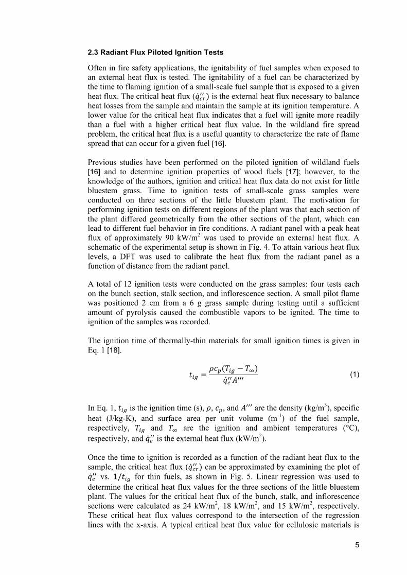
Often in fire safety applications, the ignitability of fuel samples when exposed to an external heat flux is tested. The ignitability of a fuel can be characterized by the time to flaming ignition of a small-scale fuel sample that is exposed to a given heat flux. The critical heat flux (𝑞!"!! ) is the external heat flux necessary to balance heat losses from the sample and maintain the sample at its ignition temperature. A lower value for the critical heat flux indicates that a fuel will ignite more readily than a fuel with a higher critical heat flux value. In the wildland fire spread problem, the critical heat flux is a useful quantity to characterize the rate of flame spread that can occur for a given fuel [16]. Previous studies have been performed on the piloted ignition of wildland fuels [16] and to determine ignition properties of wood fuels [17]; however, to the knowledge of the authors, ignition and critical heat flux data do not exist for little bluestem grass. Time to ignition tests of small-scale grass samples were conducted on three sections of the little bluestem plant. The motivation for performing ignition tests on different regions of the plant was that each section of the plant differed geometrically from the other sections of the plant, which can lead to different fuel behavior in fire conditions. A radiant panel with a peak heat flux of approximately 90 kW/m2 was used to provide an external heat flux. A schematic of the experimental setup is shown in Fig. 4. To attain various heat flux levels, a DFT was used to calibrate the heat flux from the radiant panel as a function of distance from the radiant panel.

A total of 12 ignition tests were conducted on the grass samples: four tests each on the bunch section, stalk section, and inflorescence section. A small pilot flame was positioned 2 cm from a 6 g grass sample during testing until a sufficient amount of pyrolysis caused the combustible vapors to be ignited. The time to ignition of the samples was recorded. The ignition time of thermally-thin materials for small ignition times is given in Eq. 1 [18].

𝑡!" =𝜌𝑐!(𝑇!" − 𝑇!)

𝑞!!!𝐴!!! (1)

In Eq. 1, 𝑡!" is the ignition time (s), 𝜌, 𝑐!, and 𝐴!!! are the density (kg/m3), specific heat (J/kg-K), and surface area per unit volume (m-1) of the fuel sample, respectively, 𝑇!" and 𝑇! are the ignition and ambient temperatures (°C), respectively, and 𝑞!!! is the external heat flux (kW/m2). Once the time to ignition is recorded as a function of the radiant heat flux to the sample, the critical heat flux (𝑞!"!! ) can be approximated by examining the plot of 𝑞!!! vs. 1/𝑡!" for thin fuels, as shown in Fig. 5. Linear regression was used to determine the critical heat flux values for the three sections of the little bluestem plant. The values for the critical heat flux of the bunch, stalk, and inflorescence sections were calculated as 24 kW/m2, 18 kW/m2, and 15 kW/m2, respectively. These critical heat flux values correspond to the intersection of the regression lines with the x-axis. A typical critical heat flux value for cellulosic materials is

6

15 kW/m2 [19]. To check the validity of the thin fuel assumption, the plot of 𝑞!!! vs. 1/ 𝑡!" for thick fuels was also examined. However, the fit of the bunch section was in better agreement when the thin fuel approximation was used, and the stalk and inflorescence sections exhibited negative values for the critical heat flux when the fuel was assumed to behave as a thermally thick material. A summary of the critical heat flux values that were calculated for the three sections of little bluestem grass is shown in Table 1. Table 1 Experimentally-determined critical heat flux values for three little bluestem grass sections Plant section Critical heat flux (kW/m2) Bunch 24 Stalk 18 Inflorescence 15 There are clear differences between the ignition times for the bunch, stalk, and inflorescence section. The bunch and inflorescence have much lower effective densities than the stalk; these lower effective densities are related to the differences in the SAV ratio (𝐴!!!) between these regions. Based upon Eq. 1, one would expect the less dense inflorescence and bunch regions to have much shorter ignition times. We see that the bunch region consistently has smaller ignition time than the stalk region, but that the inflorescence ignition time variation is less consistent. We believe that the inflorescence data is less reliable than the stalk and bunch results, because there is more judgment required in selecting the inflorescence parts of the plant. Further, much of the inflorescence is morphologically similar to the stalk regions. The differences in these values suggests that at least two different fuel models can be used to describe the physical phenomena in the wildland flame spread problem. The results also indicate that the inflorescence regions might reasonably be approximated in its behavior as the stalk regions. Therefore, in the following sections, the inflorescence and stalk regions will be considered as a combined upper region of the plant with respect to its fire behavior.

2.4 Relative Humidity and Fuel Moisture Content Measurements

In the wildland fire spread problem, an important variable in the fire spread rate is the FMC, or the amount of water present in a given fuel sample. Weather conditions can impact the rate of flame spread in a wildland fire, and elevated fire danger conditions are typically associated with low RH values along with high wind speeds. A lower RH value results in a reduced amount of moisture in vegetative fuels, and dry vegetation can result in increased fire spread rates [13,15,20-22]. The coupling of the weather conditions to the fuel can be described as a mass transfer problem from the water vapor in the gas phase (RH) to the moisture content of the condensed fuel phase (FMC). For these tests, ambient RH values were obtained from a nearby weather station located at Camp Mabry, TX at the start of each test. The moisture content of each plant was determined by removing a small sample from the plant before each test, measuring its mass, and then oven drying the sample at 101 °C. For the oven-drying process, after a two-hour period of drying at 101 °C, the grass samples were weighed at 30-minute intervals. When the mass of the samples did not

7

change significantly between weighing intervals, the dry mass of the sample was recorded, and the FMC was determined by using Eq. 2.

%  𝒎𝒐𝒊𝒔𝒕𝒖𝒓𝒆  𝒄𝒐𝒏𝒕𝒆𝒏𝒕 =

(𝒎𝒘𝒆𝒕 −𝒎𝒅𝒓𝒚)𝒎𝒅𝒓𝒚

 ×  𝟏𝟎𝟎 (2)

The resulting FMC and corresponding RH values are shown in Fig. 6. In this figure, the FMC of the samples from this study (circles) are compared to equilibrium FMC correlations (solid lines) and experimental data (triangle and square markers) for various vegetation types. The results are in good agreement with existing correlations from literature [11,23] as well as experimental data on various vegetation types [24]. As the RH decreases, the FMC of the samples also decreases. The results of these measurements indicate that, at equilibrium conditions, the FMC of little bluestem grass as a function of RH behaves similar to existing equilibrium correlations for wood and other vegetation types.

2.5 Mass Loss Experiments

In the wildland fire spread problem, the mass loss rate and burning rate of the fuel are important variables because these processes are the driving forces for combustion and flame heights, which in turn controls the rate of preheating and the pyrolysis of the unburned fuel ahead of the flame [17,25]. To characterize the mass loss rate and burning rate of the little bluestem grass samples, free-burn tests with full plants were conducted on top of an Omega Model LSC7000-20 (accuracy ±1 g) load cell with a sample resolution of 1 Hz. For these tests, excess dirt was removed from the roots before the plant was placed into a 10 cm tall PVC pipe (10 cm diameter) with the end capped. The PVC base contained approximately 500 g of sand for stability and to anchor the grass samples. For these tests, the grass samples had a mass between 39 g and 94 g. Small samples were removed from each plant to determine the FMC. For these tests, the plant and PVC base were placed on the load cell, a pilot flame was held at the base of the plant for two seconds to ignite the plant, and transient mass loss data was obtained via the DAQ as the plant sample burned. To account for the effect of various FMCs on the mass loss rate of the fuel samples, these tests were conducted on different days with RH values ranging from 29% RH to 59% RH. Figure 3a shows a photograph of the experimental setup for these tests, and a schematic of the experimental setup is shown in Fig. 7. Pictures of the burn tests were taken using a digital camera, and video of the tests was recorded at 30 frames per second using a digital video recording system. A time sequence of pictures from a burn test with an entire little bluestem grass plant is shown in Fig. 8. The resulting mass vs. time for all of the tests is shown in Fig. 9. In this figure, the mass vs. time curve of each test was normalized by its initial mass. In this figure, the plant tests are grouped by experimentally measured FMCs of 5-9% FMC, 10-14% FMC, and 15-19% FMC. The tests that used plant samples with a higher FMC exhibit a time delay before steady burning is reached, i.e., they are shifted to

8

the right in Fig. 9. Once a steady burning condition is reached (i.e., the entire plant is burning), then the mass loss rates appear to be similar. In Section 3, the results of the mass loss tests will be compared to a simple numerical flame spread model at three different FMC values (5%, 10%, and 15%).

2.6 Closed Testing for Heat Release Rate Calculation

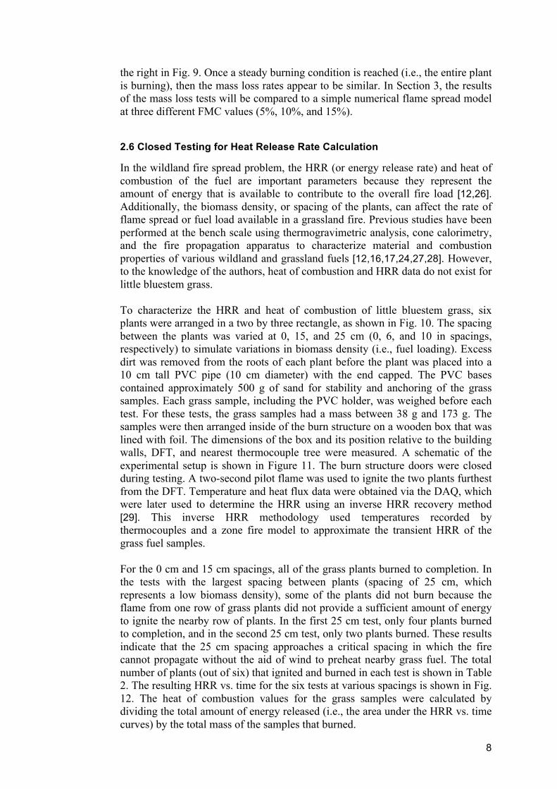
In the wildland fire spread problem, the HRR (or energy release rate) and heat of combustion of the fuel are important parameters because they represent the amount of energy that is available to contribute to the overall fire load [12,26]. Additionally, the biomass density, or spacing of the plants, can affect the rate of flame spread or fuel load available in a grassland fire. Previous studies have been performed at the bench scale using thermogravimetric analysis, cone calorimetry, and the fire propagation apparatus to characterize material and combustion properties of various wildland and grassland fuels [12,16,17,24,27,28]. However, to the knowledge of the authors, heat of combustion and HRR data do not exist for little bluestem grass. To characterize the HRR and heat of combustion of little bluestem grass, six plants were arranged in a two by three rectangle, as shown in Fig. 10. The spacing between the plants was varied at 0, 15, and 25 cm (0, 6, and 10 in spacings, respectively) to simulate variations in biomass density (i.e., fuel loading). Excess dirt was removed from the roots of each plant before the plant was placed into a 10 cm tall PVC pipe (10 cm diameter) with the end capped. The PVC bases contained approximately 500 g of sand for stability and anchoring of the grass samples. Each grass sample, including the PVC holder, was weighed before each test. For these tests, the grass samples had a mass between 38 g and 173 g. The samples were then arranged inside of the burn structure on a wooden box that was lined with foil. The dimensions of the box and its position relative to the building walls, DFT, and nearest thermocouple tree were measured. A schematic of the experimental setup is shown in Figure 11. The burn structure doors were closed during testing. A two-second pilot flame was used to ignite the two plants furthest from the DFT. Temperature and heat flux data were obtained via the DAQ, which were later used to determine the HRR using an inverse HRR recovery method [29]. This inverse HRR methodology used temperatures recorded by thermocouples and a zone fire model to approximate the transient HRR of the grass fuel samples. For the 0 cm and 15 cm spacings, all of the grass plants burned to completion. In the tests with the largest spacing between plants (spacing of 25 cm, which represents a low biomass density), some of the plants did not burn because the flame from one row of grass plants did not provide a sufficient amount of energy to ignite the nearby row of plants. In the first 25 cm test, only four plants burned to completion, and in the second 25 cm test, only two plants burned. These results indicate that the 25 cm spacing approaches a critical spacing in which the fire cannot propagate without the aid of wind to preheat nearby grass fuel. The total number of plants (out of six) that ignited and burned in each test is shown in Table 2. The resulting HRR vs. time for the six tests at various spacings is shown in Fig. 12. The heat of combustion values for the grass samples were calculated by dividing the total amount of energy released (i.e., the area under the HRR vs. time curves) by the total mass of the samples that burned.

9

The average heat of combustion from the six tests was calculated as 16.4 kJ/g (standard deviation of 3.8 kJ/g). This heat of combustion value is within the range reported in previous studies that were conducted with similar grass fuels, which is between 16.3 kJ/g and 18.5 kJ/g [30-32]. In addition to the heat of combustion, the char fraction (χ char), which is the amount of fuel that converts to char and contributes to smoldering, from each test was calculated. After each test was completed, the mass of the residual was recorded to obtain the char fraction, which was defined as the percentage of mass that remained after the sample self-extinguished. From the six closed tests, the average char fraction was calculated as 12% (standard deviation of 3%). This value compares reasonably with the char fraction values in a previous study that used Australian grassland fuels [8], which reported a char fraction of 20%. The discrepancy in the values indicates that more of the little bluestem grass is converted into combustible vapor. The resulting heat of combustion values and char fraction values are shown in Table 3. Table 2 Experimentally-determined heat of combustion and char fraction data for six grass tests Test Spacing (cm) Total number

of plants burned (out of six)

Heat of combustion (kJ/g)

Char fraction (%)

1 0 6 14.2 13 2 15 6 18.8 7 3 25 4 17.5 15 4 25 2 9.7 9 5 15 6 19.7 14 6 0 6 18.5 11

3. Intermediate-scale Flame Spread Model

3.1 Overview of Flame Spread Model

From the results of the small- and intermediate-scale experiments, we can analyze the relationship between the condensed phase fuel properties (e.g., fuel moisture content) and the fire spread rate. In the simplified flame spread problem, the pyrolysis region is the region of the fuel that produces combustible vapors at a burning rate (𝑚!

!!) that sustains the flame. Some of these fuel vapors burn above or ahead of the pyrolysis region due to buoyancy or wind effects, respectively, and the combustion that occurs above or in front of the pyrolysis region preheats unburned fuel to its ignition temperature. The virgin fuel then begins to release combustible vapors, which results in an increasing flame length. The FMC of grassland fuels and other vegetation is known to impact the flame spread rate at the full-scale (i.e., a grass field or forest). For relatively low FMCs, the rate of flame spread decreases along with an increase in the FMC. For higher FMCs, there are implications of extinction in the flame spread problem due to the effects of burnout and an insufficient amount of energy to evaporate moisture ahead of the flame front.

10

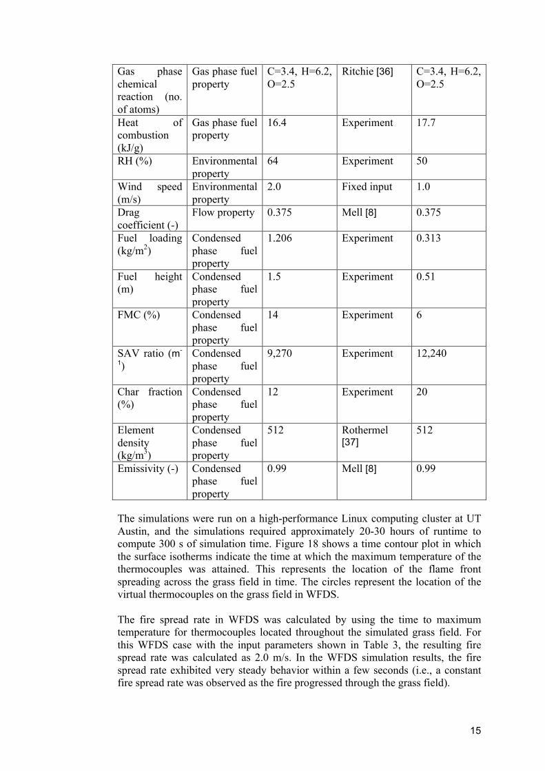
At the scale of a single fuel item (intermediate scale), Mell et al. [25] conducted experiments to measured the mass loss rate and HRR of burning Douglas fir trees with various FMCs. In those experiments, Douglas fir trees with various FMCs were ignited at the base, and the mass loss of the tree samples was recorded. The upward flame spread rate was slower for the trees with higher FMCs. In this section, the flame spread process is characterized for fuels that contain moisture, and different stages of burning are identified to understand the physical processes that occur at the intermediate scale. The full-scale flame spread problem exhibits similar physics; as a fire spreads across a grass field, the flame that extends from the pyrolysis region preheats, evaporates, and gasifies the grass fuel ahead of the flame front. For a single burning little bluestem plant, the mass vs. time from a representative intermediate-scale experiment is shown in Fig. 13. In this figure, three stages of burning are identified at their respective times: Stage 1) upward flame spread and evaporation of fuel moisture in the plant, Stage 2) steady burning of the entire plant, Stage 3) burning of only the bunch section of the plant due to burnout of the stalk section.

3.2 Model Setup

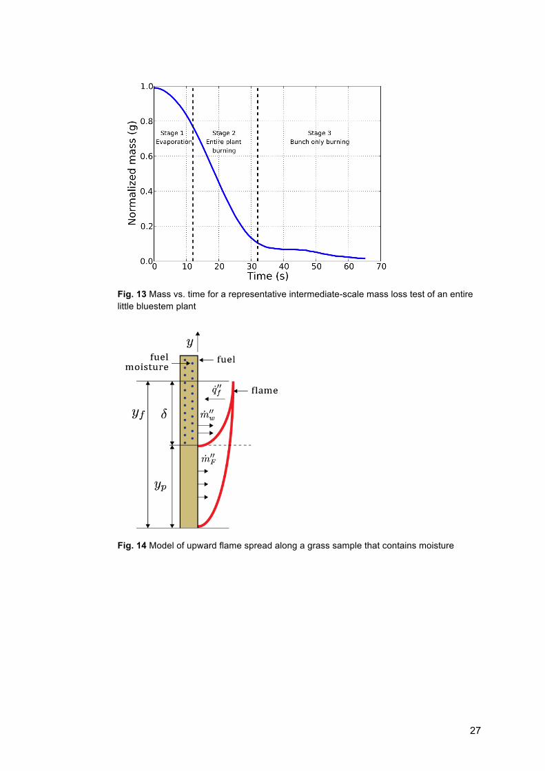
To understand the flame spread process that occurs on a single grass plant, a simple one-dimensional flame spread model was developed to predict the total mass vs. time as a function of the evaporation rate of fuel moisture and the burning rate of the fuel. A schematic of the fuel sample and the upward flame spread process on a grass plant is shown in Fig. 14. This concurrent flame spread process can be considered both at the intermediate scale for single grass plants (as discussed in this section) and at the full scale for a wildland fire. For a burning plant that contains moisture, the energy from the flame must vaporize this moisture at a rate 𝑚!! from the fuel before it ignites, which effectively increases its ignition time and decreases the rate of flame spread. In the upward flame spread problem, the pyrolysis region is characterized by the pyrolysis height (𝑦!), and the flame region is characterized by the flame height (𝑦!). The rate of spread of the pyrolysis region (𝑑𝑦!/𝑑𝑡) is defined as shown in Eq. 3.

𝑑𝑦!

𝑑𝑡 =𝑦! − 𝑦!𝑡!"!

(3)

In the flame spread model, the time step (Δt) was set to 0.1 s .In Eq. 3, the 𝑡!"! term is the total time to ignition and includes the preheating of the fuel, preheating of the moisture in the fuel, evaporation of moisture from the fuel, and preheating of the fuel to its ignition temperature, as shown in Eq. 4.

𝑡!"! = (𝜌!𝑐!∆𝑇!" + 𝜌!𝑐!∆𝑇!" + 𝜌!ℎ!" + 𝜌!𝑐!∆𝑇!"#)1

𝑞!!𝐴!!!

(4)

11

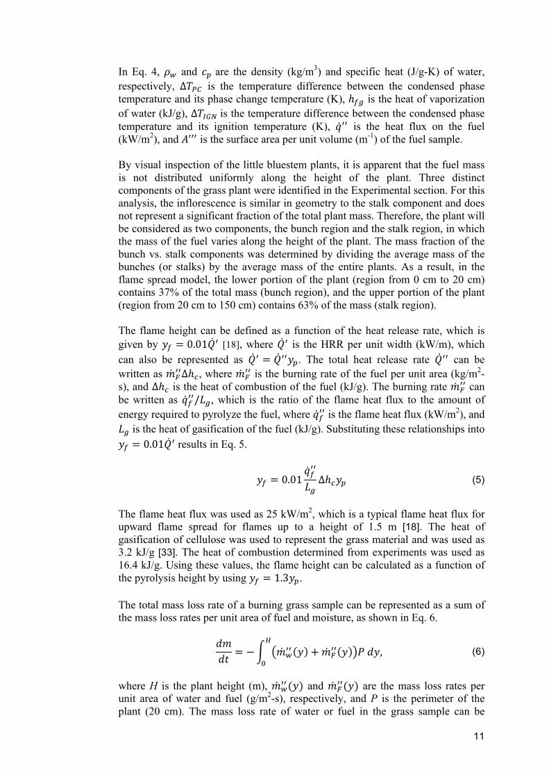
In Eq. 4, 𝜌! and 𝑐! are the density (kg/m3) and specific heat (J/g-K) of water, respectively, ∆𝑇!" is the temperature difference between the condensed phase temperature and its phase change temperature (K), ℎ!" is the heat of vaporization of water (kJ/g), ∆𝑇!"# is the temperature difference between the condensed phase temperature and its ignition temperature (K), 𝑞!! is the heat flux on the fuel (kW/m2), and 𝐴!!! is the surface area per unit volume (m-1) of the fuel sample. By visual inspection of the little bluestem plants, it is apparent that the fuel mass is not distributed uniformly along the height of the plant. Three distinct components of the grass plant were identified in the Experimental section. For this analysis, the inflorescence is similar in geometry to the stalk component and does not represent a significant fraction of the total plant mass. Therefore, the plant will be considered as two components, the bunch region and the stalk region, in which the mass of the fuel varies along the height of the plant. The mass fraction of the bunch vs. stalk components was determined by dividing the average mass of the bunches (or stalks) by the average mass of the entire plants. As a result, in the flame spread model, the lower portion of the plant (region from 0 cm to 20 cm) contains 37% of the total mass (bunch region), and the upper portion of the plant (region from 20 cm to 150 cm) contains 63% of the mass (stalk region). The flame height can be defined as a function of the heat release rate, which is given by 𝑦! = 0.01𝑄! [18], where 𝑄! is the HRR per unit width (kW/m), which can also be represented as 𝑄! = 𝑄!!𝑦!. The total heat release rate 𝑄!! can be written as 𝑚!

!!∆ℎ!, where 𝑚!!! is the burning rate of the fuel per unit area (kg/m2-

s), and ∆ℎ! is the heat of combustion of the fuel (kJ/g). The burning rate 𝑚!!! can

be written as 𝑞!!!/𝐿!, which is the ratio of the flame heat flux to the amount of energy required to pyrolyze the fuel, where 𝑞!!! is the flame heat flux (kW/m2), and 𝐿! is the heat of gasification of the fuel (kJ/g). Substituting these relationships into 𝑦! = 0.01𝑄! results in Eq. 5.

𝑦! = 0.01𝑞!!!

𝐿!∆ℎ!𝑦! (5)

The flame heat flux was used as 25 kW/m2, which is a typical flame heat flux for upward flame spread for flames up to a height of 1.5 m [18]. The heat of gasification of cellulose was used to represent the grass material and was used as 3.2 kJ/g [33]. The heat of combustion determined from experiments was used as 16.4 kJ/g. Using these values, the flame height can be calculated as a function of the pyrolysis height by using 𝑦! = 1.3𝑦!. The total mass loss rate of a burning grass sample can be represented as a sum of the mass loss rates per unit area of fuel and moisture, as shown in Eq. 6.

𝑑𝑚𝑑𝑡 = − 𝑚!

!! 𝑦 +𝑚!!! 𝑦 𝑃  𝑑𝑦

!

!, (6)

where H is the plant height (m), 𝑚!

!!(𝑦) and 𝑚!!!(𝑦) are the mass loss rates per

unit area of water and fuel (g/m2-s), respectively, and P is the perimeter of the plant (20 cm). The mass loss rate of water or fuel in the grass sample can be

12

calculated as a function of the flame heat flux, perimeter, and the heat of vaporization, as shown in Eq. 7.

𝑚!! = 𝑚!

!!𝑃 =𝑞!!!

𝐿!𝑃, (7)

where 𝑚!

! is the mass loss rate (i.e., evaporation or pyrolysis rate) of species i per unit length of perimeter around the plant (g/m-s), 𝑞!!! is the flame heat flux (kW/m2), and 𝐿! is the heat of vaporization of species i (kJ/g). As in Eq. 5, the flame heat flux was used as 25 kW/m2 [18]. For fuel moisture, the heat of vaporization of water is 2.3 kJ/g [34]. This results in a moisture evaporation rate per unit length of perimeter of 2.2 g/m-s.

Using a similar approach, the mass loss rate of the fuel was calculated using Eq. 7. The only different parameter is the heat of gasification of the fuel instead of the heat of vaporization of water. The flame heat flux and nominal plant perimeter were the same as in Eq. 7. The heat of gasification (𝐿!) of cellulose was used as 3.2 kJ/g [33]. This results in a fuel burning rate per unit length of perimeter of 1.6 g/m-s. Using this flame spread model, the presence of moisture allows for a delayed ignition time along the height of the grass samples as: (1) water is evaporated from the fuel sample elements due to heat flux from the flame, and (2) the fuel pyrolyzes and provides additional fuel mass to support the growing flame.

3.3 Flame Spread Model Results

The evolution of the pyrolysis height vs. time was calculated by integrating Eq. 3 in time. Equation 5 is then used to determine the flame height based on the pyrolysis height. The resulting pyrolysis and flame heights are shown in Fig. 15. This figure also shows a comparison of the model predictions to pyrolysis and flame heights that were recorded from the test videos Using the predicted pyrolysis and flame heights, the evolution of the total, fuel, and water mass of the plant were then calculated by time integrating Eq. 6. The results for a single plant (in which FMC = 10%) are shown in Fig. 16. In this figure, the model effectively captures the three stages of burning that were described in Section 3.1. To compare the predicted mass vs. time predicted by the flame spread model to the results of the mass loss experiments, the model was then run using three values of FMC as 5%, 10%, and 15%. The resulting mass vs. time predictions from the flame spread model were then compared to the mass vs. time data from the mass loss experiments, and the results are shown in Fig. 17. The results of the flame spread model are in good agreement with the experimental mass loss data for the range of FMCs that was considered. The flame spread model accounts for the moisture that is present in the fuel, and the model effectively captures three distinct stages of mass loss that were identified in the experiments. Additionally, the variation in the fuel mass as a function of

13

height effectively captures the two-stage burning behavior that was observed in the intermediate-scale tests with little bluestem grass plants. In the experiments, initially, the bunch region was ignited and became fully involved. The flame then quickly spread up the vertical stalk section. After the mass of the stalk sections burned away, the bunch section continued to burn, which is in agreement with observations of the two-stage burning that occurs in full-scale grassland fires. The ignition time and steady burning of the grass samples were accounted for by incorporating the moisture content of the fuel in this flame spread model. As we move towards field-scale computational fire modeling in the following section, the fire spread rate over a large grass field will be determined by using a similar concept of evaporating moisture from grass fuel followed by the pyrolysis of the fuel.

4. Numerical Modeling of a Field-Scale Burn

4.1 Description of WFDS

In this section, the results from the small- and intermediate-scale experiments will be used to develop a set of input parameters for little bluestem and predict fire spread rates at the field scale using a physics-based computational fire model. To predict fire behavior using a combination of fuel properties (as determined in this study), atmospheric conditions, and terrain properties, the computational fluid dynamics model, Fire Dynamics Simulator, was used. Fire Dynamics Simulator is a computational fluid dynamics (CFD) model of fire-driven fluid flow. FDS solves numerically a form of the Navier-Stokes equations appropriate for low-speed, thermally-driven flow with an emphasis on smoke and heat transport from fires [35]. The WFDS model refers to various submodels within the FDS framework that represent wildland fuels. Application of the WFDS model to full-scale wildfires is still in its early stages. Vegetative fuels are incorporated in WFDS by using a fuel pyrolysis submodel [25], and WFDS computes the mass loss and burning behavior of vegetative fuels in a manner similar to the intermediate-scale flame spread model that was discussed in the previous section. The vegetation submodel in WFDS accounts for moisture in the fuel, and additional fuel properties are input to specify the conditions for the heat and mass transfer processes. In a WFDS wildland fire simulation, energy from the flame preheats the unburned fuel and evaporates fuel moisture ahead of the flame front. After all of the moisture has been evaporated from the fuel in a given computational cell, that cell then releases combustible vapors at a rate dependent on the incident heat flux from the flame. The flame grows as the combustible vapors burn, which then creates a feedback mechanism for fire spread as the flame preheats additional unburned fuel ahead of the flame. As this process continues, the flame front progresses towards the unburned fuel, and the fire spread rate is modeled using a physics-based approach.

4.2 WFDS Model Setup

Texas Forest Service has conducted a series of prescribed burns at the Texas National Guard Camp Swift site. These burns were instrumented with a goal of

14

developing a site-specific fuel model. Camp Swift is an 11,470 acre site in North Bastrop County in Central Texas. Similar to the Cross Plains regions, little bluestem is the dominant grass species at Camp Swift. The WFDS model requires inputs for the terrain, weather conditions, and condensed-phase and gas-phase fuel properties. The dimensions of the field that were used as an input in the FDS model are the same as those used by TFS in their experiments. Direct comparison of the results of the experimental burns are not yet possible because the data are not yet available for public disclosure. For the terrain parameters, the dimensions of the grass field (280 m by 180 m) were input into WFDS. The height of the simulation domain was 25 m. The grid cell size used in the WFDS simulations was uniform and equal to 1.0 m on all sides. In the field-scale test burn, the flame heights were on the order of tens of meters compared to the average grass fuel height of 1.5 m. Because of the order of magnitude difference in these length scales, the grass fuel was represented in WFDS by using the boundary fuel model, which places the grass fuel along the ground plane (𝑧 = 0  𝑚). For the weather conditions, the RH, ambient temperature, and wind speed were input into WFDS as reported by a local remote automated weather station. The weather conditions at the time of the burn were input into WFDS as follows: RH of 64%, ambient temperature of 20 °C (68 °F). A fixed wind speed of 2.0 m/s (4.5 mph) was used in the simulations. This was implemented in WFDS by prescribing the boundary face along the south edge of the field with a uniform inflow velocity of 2.0 m/s. Domain boundaries other than the inflow and bottom face were prescribed as an open condition at which the density and mixture fraction have zero gradient conditions. The fuel parameters required by WFDS are as follows: gas phase reaction parameters, the heat of combustion of the fuel, drag coefficient, fuel loading, fuel height, FMC, SAV ratio, char fraction, fuel element density, and emissivity of the fuel. The fuel parameters used to represent little bluestem grass were as follows: heat of combustion, char fraction, and FMC. The heat of combustion, char fraction, and SAV ratio were determined from intermediate-scale testing, as discussed in the Experimental section. The fuel loading, grass height, and FMC were measured from grass samples taken from plots in the test field. In the WFDS simulation, the fuel type, FMC, and terrain are uniform across the grass field. In addition to the fuel properties of the grass, the ignition source was also input into the model. This was done by placing burners along the south edge of the field. Virtual thermocouples were located in the computational field and the time to maximum temperature was tracked. The parameters used in the base WFDS model are summarized in Table 3. There is very little information in the literature on WFDS and grassland fuels. For comparison, the WFDS input values from a grassland fire modeling study by Mell [8] that used Australian grass fuel are also shown in Table 3. Table 3 Fuel input properties for WFDS fire model Parameter (units)

Type Value Source Input value from Mell (2009)

15

Gas phase chemical reaction (no. of atoms)

Gas phase fuel property

C=3.4, H=6.2, O=2.5

Ritchie [36] C=3.4, H=6.2, O=2.5

Heat of combustion (kJ/g)

Gas phase fuel property

16.4 Experiment 17.7

RH (%) Environmental property

64 Experiment 50

Wind speed (m/s)

Environmental property

2.0 Fixed input 1.0

Drag coefficient (-)

Flow property 0.375 Mell [8] 0.375

Fuel loading (kg/m2)

Condensed phase fuel property

1.206 Experiment 0.313

Fuel height (m)

Condensed phase fuel property

1.5 Experiment 0.51

FMC (%) Condensed phase fuel property

14 Experiment 6

SAV ratio (m-

1) Condensed phase fuel property

9,270 Experiment 12,240

Char fraction (%)

Condensed phase fuel property

12 Experiment 20

Element density (kg/m3)

Condensed phase fuel property

512 Rothermel [37]

512

Emissivity (-) Condensed phase fuel property

0.99 Mell [8] 0.99

The simulations were run on a high-performance Linux computing cluster at UT Austin, and the simulations required approximately 20-30 hours of runtime to compute 300 s of simulation time. Figure 18 shows a time contour plot in which the surface isotherms indicate the time at which the maximum temperature of the thermocouples was attained. This represents the location of the flame front spreading across the grass field in time. The circles represent the location of the virtual thermocouples on the grass field in WFDS. The fire spread rate in WFDS was calculated by using the time to maximum temperature for thermocouples located throughout the simulated grass field. For this WFDS case with the input parameters shown in Table 3, the resulting fire spread rate was calculated as 2.0 m/s. In the WFDS simulation results, the fire spread rate exhibited very steady behavior within a few seconds (i.e., a constant fire spread rate was observed as the fire progressed through the grass field).

16

4.3 Sensitivity Analysis of the Flame Spread Rate in WFDS

From the results of the field-scale WFDS simulation, we seek to determine the effect of varying the input parameters on the calculated fire spread rate. The input parameters in Table 3 can be grouped into four categories: gas phase fuel properties, environmental properties, flow properties, and condensed phase fuel properties. Many of these input parameters can be considered to be fixed material properties or properties in which a large variation would not be expected, such as the heat of combustion of the fuel, char fraction, element density, and emissivity. For other properties that vary based on the environmental conditions or specific plot of land, or input parameters that are associated with a larger amount of measurement uncertainty, we seek to determine the sensitivity of these parameters on the resulting fire spread rate. For this purpose, we selected three input parameters to vary for this sensitivity analysis: the FMC, fuel loading, and fuel SAV ratio. Because we are interested in quantifying the impact of varying these parameters on the calculated fire spread rate, we used the fire spread rate as the output quantity to examine in the sensitivity analysis. For the sensitivity analysis, a base (reference) case was computed using the values shown in Table 3. The fire spread rate was calculated using the time evolution of the surface isotherms. Virtual thermocouples were located in the computational field, and the time to maximum temperature was tracked. The fire spread rate reached a steady value quickly. In the base case, the nominal fire spread rate was approximately 2.0 m/s. For the FMC parameter, the base case used a FMC value of 14%. To represent a range of FMCs that might be encountered in various RH conditions, two values below and two values above the FMC used in the base case were selected as 6%, 10%, 18%, and 22%. The resulting flame spread rates were between 1.4 m/s and 2.8 m/s compared to the base case flame spread rate of 2.0 m/s. The associated change in the fire spread rate as a function of the input FMC can be approximated using linear regression and is given as 𝑉 = 𝑉! + 𝑎!𝑋, where 𝑉 is the fire spread rate (m/s), 𝑉! is the fire spread rate at 0% FMC (m/s), 𝑎! is the sensitivity parameter and is equal to -0.085 m/s/FMC, and 𝑋 is the FMC (%). Using these parameters, the rate of fire spread can be calculated as a function of the FMC (ranging from 6% to 22%) for a wind speed of 2.0 m/s, as shown in Eq. 8.

𝑉 = 3.3− 0.085  ×  𝐹𝑀𝐶 (8)

This fire spread rate can be compared to a simple correlation from literature, as follows. Morvan [38] presents a simple correlation for the effect of FMC on the rate of fire spread, as shown in Eq. 9,

𝑅𝑂𝑆

𝑅𝑂𝑆(0) =𝐻!"#

𝐻!"# + 𝐻!"#  ×  𝐹𝑀𝐶100

, (9)

where 𝑅𝑂𝑆 is the rate of spread (m/s), 𝑅𝑂𝑆(0) is the rate of spread when FMC = 0% (m/s), 𝐻!"# is the amount of energy required to pyrolyze the fuel (kJ/kg), 𝐻!"# is the amount of energy required to vaporize water from the fuel (kJ/kg), and 𝐹𝑀𝐶 is the fuel moisture content (%). Using the parameters specified in

17

Morvan (𝐻!"# = 418  𝑘𝐽/𝑘𝑔; 𝐻!"# = 2,250  𝑘𝐽/𝑘𝑔), a 𝑅𝑂𝑆(0) value of 3.3 m/s, and a FMC of 14%, the rate of spread was calculated as 1.88 m/s (compared to the base WFDS case of 2.0 m/s). The resulting fire spread rate vs. FMC is shown in Fig. 19, where the circles represent the WFDS cases, and the solid line represents a linear fit to the WFDS cases. For comparison, the dashed line in Fig. 19 shows the rate of spread as a function of FMC by using Eq. 8 and the same values of HPYR and HVAP that were used in the previous section. An 𝑅𝑂𝑆(0) value of 3.3 m/s was used, which is calculated by using Eq. 9 and setting the FMC to zero. There is reasonable qualitative agreement for the fire spread rates from WFDS compared to the model by Morvan. For the fuel loading parameter, the base case used a value of 1.2 kg/m2. To represent a variation in the biomass fuel loading (fuel density) that might occur naturally in a grassland setting, one value below and one value above the base case were selected as 0.73 kg/m2 and 1.4 kg/m2, which were the minimum and maximum fuel loads that were measured at the experimental burn field. The fuel loading inputs had a range of 39% below and 17% above the base case. The resulting flame spread rates were between 1.9 m/s and 2.0 m/s for all cases, as shown in Fig. 20, compared to the base case flame spread rate of 2.0 m/s. For this range of fuel loading values, the fire spread rate did not vary significantly. For the SAV ratio parameter, the base case used a value of 9,270 m-1, which is the average SAV ratio of the entire plant. To select additional SAV ratios, we considered the minimum measured SAV ratio (stalk region) of 1,810 m-1 and the maximum measured SAV ratio (bunch region) of 11,836 m-1, as described in Section 2.2. Using increments of 1,000 m-1, three cases above the minimum (2,810 m-1, 3,810 m-1, 4,810 m-1) and two cases below the maximum (9,836 m-1, and 10,836 m-1) were selected for this sensitivity analysis. The SAV ratio inputs had a range of 70% below and 17% above the base case. For this range of SAV ratio inputs, the resulting flame spread rates were between 1.3 m/s and 2.0 m/s, as shown in Fig. 21, compared to the base case flame spread rate of 2.0 m/s. The resulting fire spread rates exhibit an exponential behavior as the SAV ratio increases rather than a linear behavior, as shown (cf. Fig. 21). However, the value used in the base case was 9,270 m-1 from measured data, which is in agreement with SAV ratio values for grass plants from literature [15]. For the range of SAV ratios from 9,000 m-1 to 11,000 m-1 for grass fuels, the fire spread rate that was calculated by WFDS did not change significantly. A summary of these WFDS sensitivity cases with different input values and the resulting fire spread rate is shown in Table 4. The results indicate that, out of the three parameters that were varied, the FMC had the most significant impact on the fire spread rate. The fuel loading and SAV ratio did not have a significant impact on the fire spread rate for the range of input values that was used. Table 4 Summary of WFDS sensitivity cases and resulting fire spread rates Case Fire spread rate (m/s) Base case (14% FMC, 1.2 kg/m2 fuel loading, 9,270 m-1 SAV ratio)

2.0

18

6% FMC 2.8 10% FMC 2.3 18% FMC 1.7 22% FMC 1.4 0.73 kg/m2 fuel loading 1.9 1.4 kg/m2 fuel loading 1.9 2,810 m-1 SAV ratio 1.3 3,810 m-1 SAV ratio 1.5 4,810 m-1 SAV ratio 1.7 9,836 m-1 SAV ratio 2.0 10,836 m-1 SAV ratio 2.0

5. Conclusions This paper discussed measurements of physical and burning characteristics of the prairie grass commonly named little bluestem. The paper noted that significant WUI fire events in Texas have largely been driven by little bluestem fueled fires. Physical properties of little bluestem were compared to properties of other grass species and wildland fuels and showed similarities. This work used small- and intermediate-scale experiments to directly parameterize a wildland fire modeling (WFDS) tool. The fire modeling tool was then used to explore the overall sensitivities of fire spread rate to fuel properties. The study conclusions are noted below. For grassland fires in low RH conditions, the fire spread rate can increase due to a reduced characteristic time for ignition of unburned grass fuel. To explore this relationship, analysis of coupled heat and mass transfer processes during grass burning was used to understand fire spread rates at both the intermediate and field scales. An intermediate-scale numerical flame spread model was developed for grass fuels that accounts for FMC to calculate the mass vs. time of a burning little bluestem plant. The intermediate-flame spread model and field-scale WFDS model effectively captured the transient flame spread problem by accounting for moisture present in the grassland fuel. In addition to the FMC characterization performed in this study, further fire tests were performed on little bluestem grass plants to understand the fuel behavior and determine combustion properties of little bluestem grass fuel in a manner consistent with existing fire safety and material flammability conventions. The radiant flux piloted ignition tests conducted with the grass samples provided a means of characterizing the fuel behavior in response to an external heat flux. The critical heat flux values for three sections of the little bluestem grass samples were determined. It was shown that little bluestem might be effectively modeled using two distinct regions. Additional parameters that describe the fuel behavior of little bluestem grass were also calculated from small- and intermediate-scale experiments, including the heat of combustion, char fraction, and SAV ratio. The heat of combustion and SAV were found to be comparable to values found in the literature for other grass species. The char fraction was approximately 40% smaller than values reported for Australian grasses.

19

The results of the experiments were used to develop input parameters for numerical simulation of a grass field using a physics-based computational fire model, WFDS. A sensitivity analysis of various WFDS input parameters was performed, and the results indicate that the FMC had the most significant impact on the fire spread rate, whereas the fuel loading and SAV ratio did not have a significant impact on the fire spread rate for the range of input values that was used. The overarching goal of this work and related work in the literature is to develop deeper understanding of the mechanisms and factors that influence wildfire evolution. With improvements to submodels and better parameterization of fuel data, physics-based fire models can more reliably be used in community preplanning and wildland fire incident management and response at the WUI.

Acknowledgements The authors acknowledge contributions from and collaboration with Karen Ridenour and Richard Gray of Texas Forest Service, Kate Crosthwaite of Texas National Guard, and Craig Weinschenk of National Institute of Standards and Technology. The authors also thank Ruddy Mell for his useful comments on the details of WFDS.

References 1. Clements C (2007) Observing the Dynamics of Wildland Grass Fires: FireFlux - A Field Validation Experiment. Americal Meteorlogical Society:1-14 2. Massada A, Radeloff V, Stewart S, Hawbaker T (2009) Wildfire risk in the wildland-urban interface: A simulation study in northwestern Wisconsin. Forest Ecology and Management 258 (9):1990-1999 3. Gray R, Dunivan M, Jones J, Ridenour K, Leathers M, Stafford K (2007) Cross Plains, Texas Wildland Fire Case Study. Texas Forest Service, 4. Inciweb (2011) Bastrop Fire Incident Overview. http://www.inciweb.org/incident/2589/. Accessed Dec. 1, 2011 5. Finney MA (2004) FARSITE: Fire Area Simulator - Model Development and Evaluation. USDA Forest Service Research Paper, RMRS-RP-4 Revised. 6. Mutlu M, Popescu S, Zhao K (2008) Sensitivity analysis of fire behavior modeling with LIDAR-derived surface fuel maps. Forest Ecology and Management 256 (3):289-294 7. Hardy C, Heilman W, Weise D, Goodrick S, Ottmar R (2008) Fire Behavior Science Advancement Plan. 8. Mell W, Jenkins M, Gould J, Cheney P (2007) A physics-based approach to modelling grassland fires. International Journal of Wildland Fire 16 (1):1-22 9. Albini F (1976) Estimating wildfire behavior and effects. USDA Forest Service, Intermountain Forest and Range Experiment Station, General Technical Report INT-30, 92 pp. 10. Anderson H (1982) Aids to determining fuel models for estimating fire behavior. USDA Forest Service, Intermountain Forest and Range Experiment Station. General Technical Report, INT-122, 22 pp. 11. Viney N (1991) A review of fine fuel moisture modelling. International Journal of Wildland Fire 1 (4):215-234

20

12. Bartoli P, Simeoni A, Biteau H, Torero JL, Santoni PA (2011) Determination of the main parameters influencing forest fuel combustion dynamics. Fire Safety Journal 46 (1-2):27-33 13. Beer T (1993) The Speed of a Fire Front and Its Dependence on Wind-Speed. International Journal of Wildland Fire 3 (4):193-202 14. Allred K (1982) Describing the grass inflorescence. Journal of Range Management 35 (5):672-675 15. Cheney N, Gould J, Catchpole W (1993) The influence of fuel, weather and fire shape variables on fire-spread in grasslands. International Journal of Wildland Fire 3 (1):31-44 16. Mindykowski P, Fuentes A, Consalvi JL, Porterie B (2011) Piloted ignition of wildland fuels. Fire Safety Journal 46 (1-2):34-40 17. Tran H, White R (1992) Burning rate of solid wood measured in a heat release rate calorimeter. Fire and Materials 16 (4):197-206 18. Quintiere JG (2006) Fundamentals of Fire Phenomena. Wiley, 19. Society of Fire Protection Engineers (2008) SFPE Handbook of Fire Protection Engineering. 4th edn. National Fire Protection Association, Quincy, MA 20. Anderson H, Rothermel R (1965) Influence of moisture and wind upon the characteristics of free-burning fires. Symposium (International) on Combustion 10 (1):1009-1019 21. Cheney N, Gould J, Catchpole W (1998) Prediction of fire spread in grasslands. International Journal of Wildland Fire 8 (1):1-13 22. Rehm R, McDermott R (2009) Mathematical Modeling of Wildland-Urban Interface Fires. Paper presented at the Mathematics and Fire Workshop, Zaragoza, Spain, 23. Sharples JJ, Mcrae RHD, Weber RO, Gill AM (2009) A simple index for assessing fuel moisture content. Environmental Modelling and Software 24 (5):637-646 24. Madrigal J, Guijarro M, Hernando C, Diez C, Marino E (2011) Estimation of Peak Heat Release Rate of a Forest Fuel Bed in Outdoor Laboratory Conditions. Journal of Fire Sciences 29 (1):53-70 25. Mell W, Maranghides A, McDermott R, Manzello S (2009) Numerical simulation and experiments of burning douglas fir trees. Combustion and Flame 156 (10):2023-2041 26. Dupuy J, Marechal J, Morvan D (2003) Fires from a cylindrical forest fuel burner: combustion dynamics and flame properties. Combustion and Flame 135 (1-2):65-76 27. Stenseng M, Jensen A, Dam-Johansen K (2001) Investigation of biomass pyrolysis by thermogravimetric analysis and differential scanning calorimetry. Journal of Analytical and Applied Pyrolysis 58-59:765-780 28. Zhang Z, Zhang H, Zhou D (2011) Flammability characterisation of grassland species of Songhua Jiang-Nen Jiang Plain (China) using thermal analysis. Fire Safety Journal 46 (5):1-6 29. Overholt KJ, Ezekoye OA (2011) Characterizing heat release rates using an inverse fire modeling technique. Fire Technology, Under Review. 30. Dalgarn M, Wilson R (1975) Net Productivity and Ecological Efficiency of Andropogon Scoparius Growing in an Ohio Relict Prairie. The Ohio Journal of Science 75 (4):194-197 31. Golley F (1961) Energy values of ecological materials. Ecology 42 (3):581-584

21

32. Kidnie S (2009) Fuel Load and Fire Behaviour in the Southern Ontario Tallgrass Prairie. Thesis, University of Toronto, 33. Lyon RE (2000) Solid-state Thermochemistry of Flaming Combustion. In: Grand AF, Wilkie CA (eds) Fire retardancy of polymeric materials. CRC Press, pp 391-447 34. Incropera FP (2001) Fundamentals of Heat and Mass Transfer. Wiley, 35. McGrattan K, McDermott R, Hostikka S, Floyd J (2010) Fire Dynamics Simulator (Version 5): User's Guide. NIST Special Publication 1019-5. National Institute of Standards and Technology, Gaithersburg, MD 36. Ritchie S, Steckler K, Hamins A, Cleary T, Yang J, Kashiwagi T The effect of sample size on the heat release rate of charring materials. In: Fire Safety Science: Proceedings of the Fifth International Symposium, 1997. pp 177–188 37. Rothermel R (1972) A mathematical model for predicting fire spread in wildland fuels. USDA Forest Service Research Paper INT-115 38. Morvan D, Méradji S, Accary G (2009) Physical modelling of fire spread in Grasslands. Fire Safety Journal 44 (1):50-61 39. Leithead HL, Yarlett LL, Shiflet TN (1971) 100 native forage grasses in 11 southern states (Agriculture handbook no. 389). U.S. Soil Conservation Service,

Figures

Fig. 1 Texas wildland fire incidents from 2001 to 2010 (courtesy of R. Gray and K. Ridenour)

22

Fig. 2 Coverage of little bluestem in Texas and the southern region of the US [39]; the shaded region indicates the presence of little bluestem grass

(a) (b)

Fig. 3 Fuel morphology of the little bluestem plant. (a) Sections of the plant classified into three sections based on geometric differences. (b) Example of branching in the little bluestem plant: first-order branching (stalk), second-order branching (inflorescence), and third-order branching (inflorescence).

23

Fig. 4 Radiant panel experimental setup used to measure ignition times for the grass fuel components

Fig. 5 1/tig vs. radiant heat flux; the x-intercept indicates the critical heat flux of the plant components

24

Fig. 6 Moisture content of grass fuel vs. RH compared to moisture equilibrium models and experimental data from literature

Fig. 7 Schematic of the experimental setup and instrumentation for the mass loss tests

6.1 m

4.88 m

Door

Grass Sample

CameraBox

Bay Doors

Load Cell

25

Fig. 8 Time sequence of mass loss test with entire little bluestem plant

Fig. 9 Normalized mass vs. time of the little bluestem plants from the intermediate-scale mass loss tests

0  cm  spacing 15  cm  spacing 25  cm  spacing

26

Fig. 10 Spacing of little bluestem stalks used in intermediate-scale HRR tests

Fig. 11 Schematic of the experimental setup and instrumentation for the HRR tests

Fig. 12 HRR vs. time for six tests with various plant spacings

6.1 m

4.88 m

Door

Grass Samples

CameraBox

Bay Doors

DFTs

SampleBox

27

Fig. 13 Mass vs. time for a representative intermediate-scale mass loss test of an entire little bluestem plant

Fig. 14 Model of upward flame spread along a grass sample that contains moisture

28

Fig. 15 Flame height and pyrolysis height vs. time from mass loss tests of entire plants, the FMC in the model was set as 10%

Fig. 16 Normalized mass vs. time for fuel mass, water mass, and total mass predicted by the flame spread model

29

Fig. 17 Normalized mass vs. time for mass loss tests of entire plants compared to model predictions for three FMC values (5%, 10%, and 15% FMC)

Fig. 18 Time evolution of the surface isotherms showing the spread of the fire front along the grass field in the WFDS simulation

30

Fig. 19 Sensitivity of the fire spread rate to the FMC

Fig. 20 Sensitivity of the fire spread rate to the fuel loading

31

Fig. 21 Sensitivity of the fire spread rate to the SAV ratio