characterization of collisional energy transfer in …

CHARACTERIZATION OF COLLISIONAL ENERGY TRANSFER IN FLOW DIAGNOSTIC

METHODS

A Dissertation

by

JOSHUA DAVID WINNER

Submitted to the Office of Graduate and Professional Studies of

Texas A&M University

in partial fulfillment of the requirements for the degree of

DOCTOR OF PHILOSOPHY

Chair of Committee, Simon North

Committee Members, Rodney Bowersox

Dong Hee Son

James Batteas

Head of Department, Simon North

August 2019

Major Subject: Chemistry

Copyright 2019 Joshua David Winner

i

ABSTRACT

The characterization of hypersonic flow fields requires an understanding of both chemical

reactions and nonequilibrium effects. While current computation models can predict behaviors for

laminar and turbulent transitions in these types of flows, experimental data is still needed to further

validate these models. Specifically, the simultaneous measurement of velocimetry and

thermometry can provide comparisons to the values of turbulent kinetic energy and turbulent heat

flux of these models.

In this work, measurements of collisional energy transfer are reported for the temperature

dependent collisional quenching of NO (A, 2Σ+) by benzene and hexafluorobenzene. Transitions

between laminar and turbulent flow behaviors could potentially be instigated with thermal

nonequilibrium in these flows. This work briefly reports on laser-induced nonequilibrium

measurements which have displayed this type of transition between flow behaviors. Two species

in particular for implementing this nonequilibrium are benzene and hexafluorobenzene. A

quantitative determination of the local number density of these molecular species for a gaseous

flow can be performed in a temperature dependent manner via collisional quenching. In this work,

measurements of collisional energy transfer are reported for the temperature dependent collisional

quenching of NO (A, 2Σ+) by benzene and hexafluorobenzene in NO/N2 flow fields.

There are a number of techniques exist for the characterization of gaseous flow fields with

simultaneous thermometry and velocimetry. In this work, a detailed error analysis of the invisible

ink nitric oxide monitoring technique is presented. This method involves the initial creation of

vibrationally excited NO seeded into a flow with two subsequent “read” measurements; one

mapping displacement of the original position of the vibrationally excited NO and a second “read”

ii

step to map a second distinct rotational state of NO laser induced fluorescence, providing a

temperature measurement. This analysis was performed with a comprehensive kinetics program

which both tracks the vibrational excitation of all species present in a flow field as well as the

thermal perturbation caused by the invisible ink method. This analysis was performed for three

distinct flow facilities located at the National Aerothermochemistry Lab; a pulsed hypersonic test

cell, a supersonic high Reynold’s number facility, and a high enthalpy expansion tunnel.

iii

ACKNOWLEDGEMENTS

I would like to thank my Ph. D. advisor, Dr. Simon North, for his mentorship, patience in

helping me, and constant support of my scientific future. His ability to take complex topics and

explain them in simple ways has taught me so much about the nature of sharing scientific

knowledge. I hope in the future to help others understand science through the same methods and I

feel I have learned so much in how to communicate and present science from him, as well as of

course the science itself. I would also like to thank my committee (which has been quite extensive

over the years), including Dr. Rodney Bowersox for always finding time in his busy schedule to

provide insight and help, Dr. Stephen Wheeler, Dr. Robert Lucchese, Dr. Dong Hee Son, and Dr.

James Batteas.

There are so many to thank who drove me to science over the years. From my early days

in math and science, I want to thank my mother and father, who provided constant support in my

desire to learn as well as a stable environment where I never had to worry about hunger or money.

They gave me every opportunity to explore my interests and always provided encouragement and

support. There are many teachers over the years who encouraged me to pursue science and I am

forever grateful to them, since I have seen in my own experience a good teacher can mean a great

deal to the self-esteem of a child. I’d like to specifically thank Ms. Whelan, Ms. Rickman, Ms.

Weitkamp, Ms. Boulanger, Ms. Hoffman, Ms. Legere, and Mr. Klaene, although there are

countless others that should be thanked. I would also like to thank my professors at Centre College,

specifically those in chemistry and mathematics. Doctrina lux mentis. I’d like to specifically thank

Dr. Montgomery, Dr. Muzyka, Dr. Paumi, Dr. Haile, Dr. Miles, Dr. Wiglesworth, Dr. Swanson,

Dr. Heath, and Dr. Wilson.

iv

From the moment I arrived for graduate school at Texas A&M University, I’ve been

welcomed by countless people. I can say without my friends here, I may never have made it this

far. I’d like to thank Tom Malinski, Tom O’Loughlin, Kelsey Schulte, David and Becca Kempe,

Chris Watson, Alex Trott, Lauren Washburn, Liz Stewart, Seth and Corrin Corey, Ryan Coll, Ryan

Sarkisian, Greg Waetzig, Chris Komatsu, Alex Kalin, Corey Burns, Brad Scurria, Johnny and Tori

Graham, Mike Eller, and all my friends over these last five years. They have made College Station

feel like a true home.

The North research group has been an amazing environment to work in and the members

of this group have provided an amazing environment for science and happiness. I want to thank

my mentor, Dr. Niclas West, for teaching me all about what it takes to run successful experiments,

to embrace the grind, and to not focus on negatives. I would like to thank Madison McIlvoy for

both the three years of experiments together as well as an amazing friendship. I can only hope we

end up reunited on a research project in the future, getting each other motivated through late night

experiments. I want to thank Dr. Rodrigo Sanchez-Gonzalez, for years of advice, patience and

unique opportunities at collaboration. I would like to thank Colin Wallace, for always providing

sound advice and unique perspectives. His work drove me to try and keep up. I want to also thank

Dr. Michelle Warter, who always appreciated lab sculptures and tree climbing, Dr. Wei Wei, who

was a constant joker around the office with an incredible understanding of his science, Carolyn

Gunthardt, who was a welcome addition to the North group and always kept the best inside jokes

of the office, Zach Buen, who is one of the most uniquely positive people I have ever met, and has

a very bright future as he takes over chemistry projects at the NAL, Jason Kuszynski, Alex

Prophet, Caroline Loe, and all the undergraduates who helped me in lab over the years, Madeline

Smoltzer, who has been the best first year a mentor could ask for, with a curiosity for science as

v

well as an uplifting personality, and Megan Aardema and Nick Shuber, who both have bright

futures in the North group and chemistry in general.

Lastly, I want to thank all the staff at Texas A&M for dealing with much of headaches of

the academic world. I would like to specifically thank Will Seward in the machine shop for both

teaching me the basics of metal working as well as always making our custom pieces incredibly

fast and with a clever joke. I want to thank Sandy Horton and Valerie McLaughlin for always

providing a calm answer to any questions about expectations or paperwork and working tirelessly

on behalf of the graduate students at A&M. Lastly, I’d like to thank Tim Pehl in the electronics

shop for all his advice and help in building custom circuits for our experiments. He was always

practical in advice and quick to help, no matter how large his workload had become.

vi

CONTRIBUTORS AND FUNDING SOURCES

Contributors

This work was supervised by a dissertation committee consisting of Professor Simon North

[advisor], Professor Dong Hee Son, Professor James Batteas of the Department of Chemistry and

Professor Rodney Bowersox of the Department of Aerospace Engineering.

The laser control programs and temperature analysis programs described in Chapter 2 were

predominantly written by Dr. Niclas West, with minor changes from various students in the North

group. The gas injection system utilizing fuel injectors was originally designed by Josh Winner,

Feng Pan, and Brianne McManamen. The fabrication of this design was done by Will Seward. The

further characterization of their performance was done by Alex Prophet, Josh Winner, and Dr.

Rodrigo Sanchez-Gonzalez.

The LINE measurements described in Chapter 3 were taken by Dr. Niclas West and Josh

Winner at 300 K. Detailed modelling of these systems was performed by Dr. Amit Paul and Dr.

William Hase at Texas Tech University, along with advice on the modelling included with the

original publication of this work. The quenching measurements described in Chapter 3 were

performed by Josh Winner and Madison McIlvoy at 300 K and for the low temperature benzene

measurements. The low temperature quenching by hexafluorobenzene was measured by Dr. Niclas

West.

The computational model in Chapter 4 was initially designed by Dr. Simon North and Feng

Pan. All coding and calculations presented in this chapter was performed by Josh Winner. Some

of the methodology was a result of discussions with Dr. William Hase at Texas Tech University,

specifically with the discussion of stiff systems of differential equations presented in Chapter 5.

vii

Values for the HXT facility were obtained from Dr. Rodney Bowersox, who also provided the

Fortran code used for the thermodynamic equilibrium calculations presented in Chapter 4.

The fluorescence images shown in Chapter 5 for the SHR facility were measured by Dr.

Rodrigo Sanchez-Gonzalez, Feng Pan, and Brianne McManamen, and the ACE fluorescence

images were measured by Zachary Buen and Madeline Smoltzer. The NO injection system was

designed by Dr. Rodrigo Sanchez-Gonzalez, Feng Pan, Josh Winner, Zachary Buen, and Casey

Broslawski.

All other work conducted for this dissertation was completed by Josh Winner under the

advisement of Dr. Simon North.

Funding Sources

Graduate study was supported by a fellowship from Texas A&M University.

This work was also made possible in part by the United States Air Force Office of

Research, under Grant Number C13-0027, as well as Grant Number FA9550-17-1-0107. Its

contents are the sole responsibility of the authors and do not necessarily represent the official views

of the United States Air Force Office of Research.

viii

NOMENCLATURE

NAL National Aerothermochemistry Lab

LINE Laser Induced Non-Equilibrium

VENOM Vibrationally Excited Nitric Oxide Monitoring

PIV Particle Image Velocimetry

MTV Molecular Tagging Velocimetry

PLIF Planar Laser Induced Fluorescence

FRS Filtered Rayleigh Scattering

FLEET Femtosecond Laser Electronic Excitation Tagging

STARFLEET Selective Two-Photon Absorptive Resonance Femtosecond Laser

Electronic Excitation Tagging

LIF Laser Induced Fluorescence

BBO Barium Borate Crystal

PMT Photomultiplier Tube

MCP Micro Channel Plate

CCD Charge Coupled Device

ICCD Intensified Charge Coupled Device

RET Resonant Energy Transfer

FHO Forced Harmonic Oscillator

VV Vibrational-Vibrational Energy Transfer

VT Vibrational-Rotational/Translational Energy Transfer

PHT Pulsed Hypersonic Test Cell

SHR Supersonic High Reynolds Number Flow Facility

ix

HXT High Enthalpy Expansion Tunnel

ACE Actively Controlled Expansion Tunnel

RK Runge-Kutta Method

x

TABLE OF CONTENTS

Page

ABSTRACT .............................................................................................................................. ii

ACKNOWLEDGEMENTS ...................................................................................................... iv

CONTRIBUTORS AND FUNDING SOURCES .................................................................... vii

NOMENCLATURE ................................................................................................................. ix

TABLE OF CONTENTS .......................................................................................................... xi

LIST OF FIGURES .................................................................................................................. xiii

LIST OF TABLES .................................................................................................................... xviii

CHAPTER I INTRODUCTION ......................................................................................... 1

I.1 Background and Motivation .......................................................................................... 1

I.2 Research Objectives ...................................................................................................... 3

I.3 Literature Survey ........................................................................................................... 3

I.3.1Hypersonics and Direct Numerical Simulations ................................................... 3

I.3.2 Velocity Measurements in Gas Flows .................................................................. 6

I.3.3 Thermometry and Combined Measurements in Gas Flows ................................. 7

I.4 Theoretical Background ................................................................................................ 11

I.4.1 Laser Induced Fluorescence ................................................................................. 11

I.4.2 Nitric Oxide Spectroscopy .................................................................................... 15

CHAPTER II EXPERIMENTAL METHODS AND EQUIPMENT ................................... 21

II.1 Description of Laser System ........................................................................................ 21

II.2 Calibration of Laser System ......................................................................................... 23

II.3 Laser Induced Fluorescence Calibration ...................................................................... 24

II.4 Detection Systems ........................................................................................................ 28

II.5 Temperature Analysis Program .................................................................................... 29

II.6 Gas Injection System .................................................................................................... 31

CHAPTER III CHARACTERIZATION OF TEMPERATURE DEPENDENT COLLISIONAL

QUENCHING OF NO (A 2Σ+) BY BENZENE AND

HEXAFLUOROBENZENE .......................................................................... 35

III.1 Previous LINE Measurements .................................................................................... 35

xi

III.2 Experimental Method.................................................................................................. 39

III.3 Results and Analysis ................................................................................................... 47

III.4 Conclusion .................................................................................................................. 63

CHAPTER IV A COMPREHENSIVE ANALYSIS OF THE APPLICABILITY OF THE

INVISIBLE INK VENOM METHOD .......................................................... 64

IV.1 Introduction ................................................................................................................ 64

IV.2 Model Description ...................................................................................................... 67

IV.2.1 Initial Generation of Vibrational/Rotational/Translational Excitation in NO ... 67

IV.2.2 Kinetic Model of Vibrational Thermalization and Temperature Perturbation .. 73

IV.3 Results and Discussion ............................................................................................... 76

IV.3.1 Pulsed Hypersonic Test Cell .............................................................................. 77

IV.3.2 Supersonic High Reynolds Number Flow Facility ........................................... 83

IV.3.3 High Enthalpy Expansion Tunnel ...................................................................... 89

IV.4 Conclusion ................................................................................................................. 98

CHAPTER V CONCLUSION AND FUTURE WORK ...................................................... 100

V.1 NO Injection in Hypersonic Wind Tunnels ................................................................. 100

V.2 Low Temperature Collisional Quenching with Polar Quenchers ................................ 109

V.3 Future Updates to Kinetic Simulations for HXT and SHR .......................................... 110

REFERENCES ......................................................................................................................... 115

xii

LIST OF FIGURES

FIGURE Page

1.1 Two-level LIF diagram, including manifolds of vibrational and rotational energy

levels ................................................................................................................. 12

1.2 The molecular orbital diagram of NO ........................................................................ 16

1.2 The total angular momentum (J) of NO is a combination of the projections of the

spin (Σ) and orbital (Λ) angular momentum and the nuclear rotation (N),

which is perpendicular to the bond axis for Hund’s case (a) ............................ 18

1.3 The total angular momentum (J) of Hund’s case (b) is a combination of the spin

angular momentum (S), and the quantum number (K), which itself is a

combination of nuclear rotation (N) and orbital angular momentum (Λ) ........ 19

1.5 An energy level diagram for the 12 branches of the NO A-X system ....................... 20

2.1 An image of the laser resonator for the previously described laser system. The

two reflecting plates are labelled, along with the laser beam path and stepper

motor connection .............................................................................................. 22

2.2 An example of a Gaussian fitting to a measured intensity peak when scanning

the frequency conversion unit of a laser vs. the produced 226 nm intensity .... 23

2.3 A sample plot of a scan of the frequency conversion unit motor position vs. the

wavelength produced by the laser at the location of maximum signal. For

both laser systems previously described, the best fit function is a first-order

polynomial ........................................................................................................ 24

2.4 An image of the BBO contained in the FCU of the laser system. The red arrow

signifies where the stepper motor is changing positions as the motor position is

scanned .............................................................................................................. 24

2.5 A diagram of the calibration cell used for the scanned laser systems ....................... 25

2.6 A sample of a trace collected from the power correction PMT system as well as

an integration of the power correction system over a specified scanning

range. The vertical solid green and red bars correspond to the range within

the trace that is integrated and is tunable for the experiment. The dashed

green and red lines represent the region of background signal, used for

correction. ......................................................................................................... 26

xiii

2.7 A sample spectrum for NO LIF from LIFBASE. This model is for a temperature

of 56 K and line resolution of 0.01 nm. Both of these parameters are tunable

within the program ............................................................................................ 27

2.8 A sample measurement of measured rotational populations vs. rotational energy.

The linear fit corresponds to a temperature of 92.7 K. The measured

fluorescence scan is shown in the top right corner, and the relevant J-state of

each peak and point are labelled ....................................................................... 31

2.9 A comparison of experimentally measured time resolved pressure traces compared

to Gauss error function fittings. The experimental data is represented by the

dotted traces, while the fits are the solid colored lines ..................................... 32

2.10 A measurement of the flow rate dependence on backing pressure. The data is fit

with a least-squares linear function. Error bars are displayed, but error in the

flow rate calculation was found to be < 4% for all backing pressures tested ... 34

3.1 A plot showing an experimental temperature rise at 18 torr compared to an energy

independent model for α and an energy dependent model for α ....................... 37

3.2 Experimental LIF spectrum for NO (X->A). The bands measured were Q2 + R12

and P2 + Q12 and the specific j-states used for temperature fitting are

labelled. This fluorescence scan is for a sample at approximately 300 K ........ 41

3.3 The measured absorbance spectrum of benzene performed in this work compared

to a previous measurement by Olive [65, 66]. The spectrum from Olive and

coworkers has been Gaussian blurred to match the experimental resolution

from this work ................................................................................................... 43

3.4 A comparison of the spectrum from Olive [65, 66] to the Gaussian blurred version

of the spectrum used for comparison to the experimental measurements

taken in this work .............................................................................................. 44

3.5 A Beer’s law plot of benzene absorption at 238.3 nm vs. benzene concentration.

The linear fit has an R2 = 0.9927 with the experimental data and the fit is

forced through the origin .................................................................................. 45

3.6 NO fluorescence intensity vs. laser power. The intercept of the linear fit is fixed

through the origin. The fluorescence is from j = 10.5 in the R12(1.5), Q2(1.5)

band, although multiple rotational states were measured and found to be

similarly linear .................................................................................................. 46

xiv

3.7 Representative fluorescence decays in this experiment. These specific decays

were measured for NO (A 2Σ+) with benzene quenching at 300 K. Three

different experimental benzene concentrations are displayed. One in ten

points experimentally collected are displayed here for clarity ......................... 47

3.8 A plot of total measured decay rate vs. quencher number density for experimental

measurements at 300 K. The black data is for benzene and the red is for

hexafluorobenzene ............................................................................................ 51








measurements at 177 K for benzene and 155 K for hexafluorobenzene. The

black data is for benzene and the red is for hexafluorobenzene ....................... 54

3.12 A plot of experimentally determined quenching cross section vs. the electron

affinity of the quenching partner for NO (A 2Σ+) quenching ............................ 56

3.13 A plot of experimentally measured quenching cross sections for molecules

expected to undergo the resonant energy transfer mechanism for quenching

vs. calculated capture cross sections ................................................................. 60

3.14 A plot of collisional quenching cross section vs. temperature for the experiments

performed in this work. The black circles represent benzene measurements

and the blue squares represent hexafluorobenzene measurements. The

dotted lines correspond to the least squares fitting of the function σ = A*TB . . 61

3.15 A plot of experimentally determined quenching cross sections with NO (A 2Σ+)

vs. the integrated spectral overlap between the emission spectrum of NO

(A 2Σ+) and the absorption spectrum of the quencher ....................................... 62

4.1 A typical timing diagram of a VENOM measurement .............................................. 65

4.2 An energy level diagram of the invisible ink VENOM method ................................ 66

4.3 A comparison of the vibrational population distribution measured by Hancock

and Saunders [96] to the vibrational distribution predicted by the prior

probability model for a single quenching collision of NO (A 2Σ+) with a

diatomic partner ................................................................................................ 71

xv

4.4 A comparison of the vibrational populations produced by fluorescence and

collisional quenching for relaxation of NO (A 2Σ+) .......................................... 72

4.5 This plot displays the vibrational relaxation of v = 0-22 in the PHT facility for 2%

NO seeding at the conditions previously described. The times given in the

legend refer to the time delays after the initial “write” laser of the invisible

ink method. The black data represents the final vibrational distribution

expected at thermodynamic equilibrium ........................................................... 80

4.6 A plot of NO (X, v=1) over time immediately after relaxation of NO (A, 2Σ+) via

quenching and fluorescence. The long total rethermalization time (~400 ms)

should be noted ................................................................................................. 83

4.7 Predicted fluorescence decay rates for the PHT, SHR and HXT flow facilities,

along with the intrinsic rate of fluorescence for NO (A, 2Σ+). All decay rates

were calculated for the conditions listed in Table 4.1, utilizing 5% NO

seeding .............................................................................................................. 85

4.8 A plot of the time-dependent temperature rise in the SHR facility using a NO seed

concentration of 5%. The short-term and long-term temperature rises are

separated by vertical dotted lines and clearly display two distinct time

regimes .............................................................................................................. 86

4.9 An experimental diagram of the HXT facility. The acceleration region has been

truncated for posting here. The conditions and regions of the facility are

clearly labelled .................................................................................................. 90

4.10 This plot displays the predicted concentration of NO in the HXT flow facility for

a range of flow temperatures. This was determined through a

thermodynamic equilibrium calculation [109] .................................................. 91

4.11 This plot shows the time dependence of the two different simulations of NO

(X, v=1) in the HXT facility. The dotted black vertical line is included for

clarifying the timescale of a VENOM measurement on the logarithmic

“time” axis ........................................................................................................ 95

4.12 A plot of the time dependent evolution of NO (X, v=1) following the “write” laser

pulse in the invisible ink VENOM method. The dotted horizontal line refers

to the vibrational population at the final vibrational temperature of the flow

of ~349 K. The shaded region represents the additional population of NO

(X, v=1) resulting from the “write” laser excitation ......................................... 97

5.1 An image of the fuel injector containment cell used for injecting NO into the ACE

and SHR facilities ............................................................................................. 101

xvi

5.2 Fluorescence images of the “write” and “read” laser fluorescence in the SHR

velocimetry measurement. For these measurements, t0 refers to the time of

the initial “write” laser entering the flow field ................................................. 102

5.3 The experimental layout of the NO injection system tests in the SHR facility ......... 103

5.4 The determined one-dimensional velocity in the SHR facility for the testing of the

NO injection system .......................................................................................... 104

5.5 The first and second versions of the NO injection pipe used for the ACE facility.... 105

5.6 Images of NO fluorescence within a single run in the ACE facility. ........................ 107

5.7 Three images of NO fluorescence from a small laser sheet in the ACE facility.

The flow direction is from the top of the image to the bottom ......................... 108

xvii

LIST OF TABLES

TABLE Page

3.1 This table is a summary of the calculated quenching cross sections measured in

this work. The error bars are a result of 2σ error .............................................. 55

4.1 This table lists the experimental conditions for each flow facility considered in this

work as well as several experimental constants used in the kinetic

calculations that follow ..................................................................................... 77

4.2 This table displays the calculated short time (Trapid) and long time (Tfinal)

temperature rises due to the invisible ink method for three different seed

concentrations of NO. QF Ratio refers to the ratio of quenching to

fluorescence for a given set of conditions ......................................................... 81

4.3 This table displays the short-term and long-term temperature rises calculated for

the SHR flow facility for a range of NO seed concentrations. Also of note is

the ratio of quenching to fluorescence for these flow conditions, represented

by QF Ratio. Trapid is due to electronic quenching and subsequent

rotational/translational rethermalization while Tfinal includes the final

long-time (> 1 ms) flow temperature after vibrational rethermalization .......... 87

5.1 This table lists quenchers of NO (A, 2Σ+) which are predicted to act via RET,

along with their respective dipole moments ..................................................... 110

1

CHAPTER I

INTRODUCTION

I.1 Background and Motivation

The National Aerothermochemistry Lab (NAL) at Texas A&M University is an

interdisciplinary facility which functions as a collaboration between the Chemistry and Aerospace

Engineering departments. This facility is concerned with characterizing the coupling of fluid

dynamic processes various forms of thermal non-equilibrium as well as chemical kinetic processes.

This involves both experimental measurements of flow fields and theoretical modelling of these

processes. Thermal non-equilibrium is known to play a major role in hypersonic flow conditions,

where different flow processes cannot reach a single Boltzmann temperature on the timescale of

the flow. This type of non-equilibrium includes shock waves, where there is a rapid rise in the

rotational/translation temperature within the flow, but a much slower rise of vibrational

temperature. Because of different temperature phenomenon in hypersonic flows, certain

assumptions are regularly used in computational models to predict basic flow characteristics.

These models can fail when describing these flows across a wide range of spatial and temporal

timescales required to fully characterize these different time-scale non-equilibrium processes.

Specifically, turbulent processes in hypersonic flows have a strong dependence on thermodynamic

processes across the flow. To properly evaluate computational models of hypersonic turbulent

flows, correlated measurements involving both these thermal non-equilibrium processes as well as

basic turbulent processes (turbulent kinetic energy, spatially resolved velocity, etc.) need to be

performed.

2

Previous measurements of non-equilibrium processes have involved laser induced non-

equilibrium (LINE) to create vibrationally excited molecules in flow fields [1]. The goal of these

studies was to create gradients of vibrational temperature across a flow. The freestream vibrational

excitation is predicted to occur much slower than the vibrational excitation at a wall. This will

create a gradient of vibrational temperatures in the flow, which could then induce turbulent

behaviors. Another LINE study involves the preparation of vibrationally excited benzene and

hexafluorobenzene molecules and monitoring of the subsequent vibrational to

rotational/translational energy transfer with N2 [2]. The authors found a gradient of benzene and

hexafluorobenzene in their tested flow fields. It would be beneficial to develop a methodology for

determining the number density of a particular collisional energy transfer partner in a spatially

resolved and temperature dependent manner. This thesis includes the measurement of temperature

dependent quenching cross sections for benzene and hexafluorobenzene for the purposes of

characterizing these number densities.

Furthermore, the study of non-equilibrium effects in hypersonic flow fields requires

correlated measurements of flow temperature modes and velocity. The vibrationally excited nitric

oxide monitoring technique (VENOM) has previously shown the ability to make these types of

measurements [3, 4]. More recently, a new variant of this method, dubbed the “invisible ink”

method, has been used to reduce the flow perturbation of this technique as well as improve the

accuracy of the temperature measurements [5]. This thesis presents a full error analysis of this new

technique with a comprehensive kinetics study of the processes occurring in three distinct

hypersonic flow facilities present at the NAL.

3

I.2 Research Objectives

The main objectives of this work were (1) the measurement of temperature dependent quenching

behavior for benzene and hexafluorobenzene, which can allow for spatially resolved determination

of molecular number densities in flow fields, and (2) a full analysis of the novel “invisible ink”

method and the expected temperature perturbation and performance of the method in three distinct

flow facilities at the NAL.

I.3 Literature Survey

I.3.1 Hypersonics and Direct Numerical Simulations

Hypersonic flow fields exhibit several unique characteristics when compared to both sub-sonic

and supersonic flows. While all supersonic flows can exhibit hypersonic properties to some extent,

these effects are usually considered negligible. A flow field can be considered hypersonic with

Mach numbers ranging from 3 – 12 if there are significant effects from entropy layers, kinetic

heating, viscous interactions, low density flows, and thin shock layers [6]. The discussion in this

thesis will focus on the effects of entropy layers and kinetic heating.

Entropy layers occur for most hypersonic vehicles due to curved detached shocks on these

vehicles [7]. For a curved shockwave, there is are separate regions of the shockwave; a normal

shock region results in the kinetic motion of the gas molecules being converted to enthalpy and a

decrease in pressure, while parallel shock regions undergo less heating and are higher in pressure

than the normal shock region. The gradient between these two regions leads to an entropy layer,

where these two scalars vary across the spatial range of a shock. Characterization of an entropy

layer requires spatially resolving both the kinetic motion of the gases present as well as the

enthalpy of the gas.

4

Kinetic heating for a hypersonic vehicle occurs at the boundary layer of the flow field. The

state of the boundary layer (whether it is laminar or turbulent) will greatly affect the rates of heat

transfer, since turbulent behaviors result in a much higher rate of mixing. Furthermore, the state of

a boundary layer is impacted by factors such as the wall temperature and the rate of heat transfer

[8]. Because of the coupled nature of these effects, it is important to discuss the recovery

temperature of the hypersonic flow at a wall all well as effects from thermal non-equilibrium due

to the varying rates of heat transfer.

Recovery temperature can be described by the equation

𝑇𝑅 = 𝑇𝐵𝐿 (1 + 𝑅(𝛾 − 1)𝑀2

2)

(Eq. 1.1)

where TR is the temperature recovered at the wall, TBL is the temperature at the boundary layer

edge, R is the recovery factor of the flow, γ is the ratio of heat capacities of a gas (for air, γ = 1.4),

and M is the Mach number at the boundary layer edge [9]. The recovery factor of a flow can be

estimated by the equation

𝑅 = 𝑃𝑟𝑛 (Eq. 1.2)

where Pr is the Prandtl number of a flow and n is ½ for a laminar boundary layer and 1/3

for a turbulent boundary layer. The Prandtl number is a ratio of the viscous diffusion rate of a gas

to the thermal diffusion rate of a gas (for air, Pr = 0.71). The value of recovered temperature, TR,

can be thought of as the highest temperature experienced by the wall.

As previously mentioned, differences in energy transfer rates for hypersonic flows can also

lead to high temperature effects. For example, in shock tube flows, gas samples can be prepared

at temperatures > 2000 K prior to hypersonic expansion. While the hypersonic expansion will

convert the specific enthalpy of the gas into kinetic motion, vibrational temperatures of the gas

molecules normally relax at slower rates (~103 – 104 collisions) than rotational and translational

5

temperatures (< 10 collisions). Therefore, it is important to characterize all forms of thermal non-

equilibrium present, and make the distinction between rotational/translational excitation, and

vibrational excitation.

The current state of direct numerical simulations of hypersonic boundary layers and

transitions in these layers involves solving for systems where the Navier-Stokes equations are

valid. Most studies are concerned with low-enthalpy hypersonic flows based on the perfect gas

model of these equations, which match the conditions of most experimental wind tunnels [10].

However, for hypersonic flows with high enthalpy, real gas effects become a significant

consideration. This includes vibrational excitation, dissociation and recombination processes,

ionization, and radiative emission [11]. The development of non-equilibrium hypersonic flow

solvers has been a point of significant focus [12-16] as well as the validation of these solvers [17].

Most of these studies are performed for hypersonic flows across simple geometries, such as sharp

wedges or flat plates. For more complex shapes, there are various types of numerical methods for

solving the more complex flow characteristics that can arise [10]. While the field has advanced

significantly in recent years, experimental studies on the transitions of hypersonic boundary layers

which include real gas effects have been limited [18, 19] and many physical mechanisms in these

transitions are poorly understood. Therefore, experimental measurements of quantities produced

by direct numerical simulations are required to further validate the various numerical methods of

solving the Navier-Stokes equations. This work in this thesis is based around the experimental

measurement of both the turbulent kinetic energy of a system as well as the turbulent heat flux.

These measurements require the simultaneous correlated measurement of temperature of a flow as

well as the three-component velocity of a flow.

6

I.3.2 Velocimetry Measurements in Gas Flows

There are several existing methods for measuring spatially resolved velocity in a gas flow.

Particle image velocimetry (PIV) involves seeding a flow with tracer particles to track the flow

behavior at various time delays [20-22]. This method requires the tracer particles accurately

tracking the velocity of flow molecules. This requirement can be an issue in flows with strong

gradients, where the rapid movement of gas molecules occurs significantly faster than the

subsequent movement of the tracer particles [23].

Another method of velocimetry is molecular tagging velocimetry (MTV) [24, 25]. This

method is performed by seeding molecules into a flow field that can initially be tagged in some

way that permits tracking via a second “read” step. The displacement from the initial tagging

position to the subsequent “read” position is then used to determine velocity. Since the tracer

species used for MTV are normally small molecules, as opposed to the large tracer particles

normally used in PIV, these tracers in MTV can provide accurate velocimetry across strong

velocity gradients and shock waves. Furthermore, unlike PIV, MTV does not require uniform

seeding of the tracer molecule. There are several methods for this initial tagging step as well as the

subsequent “read” step. The Raman-exciting laser-induced fluorescence (RELIEF) uses Raman

scattering to create vibrationally excited molecular oxygen, which then can be electronically

excited after some time delay to prove the “write”-“read” measurement [26-28].

The inherent fluorescence lifetime of a molecule can also be used for velocimetry, by

monitoring the spatial displacement of the fluorescing molecules over time. This has been done

for high Mach number flows in the past, utilizing NO, where an initially written line of

electronically excited NO is subsequently detected at some time delay to then provide a velocity

measurement [29].

7

The tagging step in MTV can also involve photodissociation processes to create non-

equilibrium energy states to later be probed. Methods such as NO2 photodissociation have been

used at a range of “write” wavelengths to create regions of NO in a flow [30, 31]. The NO can

then be subsequently probed for a time-delayed velocity measurement.

I.3.3 Thermometry and Combined Measurements in Gas Flows

There are several experimental methods utilized in the characterization of

rotational/translational temperatures in gas flow fields. Planar laser-induced fluorescence (PLIF)

is a common and well established technique for determining spatially resolved two-dimensional

maps of rotational/translational temperature utilizing a tracer species [32, 33]. This method

measures the relative populations of two distinct rotational states of the tracer species in a flow.

The relative population of the two states can then be used to calculate a flow temperature via a

Boltzmann model on a pixel-by-pixel basis. This method does normally require seeding of the

tracer species in a flow if it is otherwise not present. However, uniform flow seeding is not

required, since the two images taken eliminate local tracer number density effects. This technique

has been recently extended to single-image methods by employing structured imaging analysis,

where one of the two “read” laser sheets is periodically modulated in intensity and overlapped

spatially and in time with the second “read” laser sheet [34]. Subsequent frequency filtering of the

single resulting fluorescent image can then be performed to provide corrected images of the two

distinct energy states, with the resulting temperature map being comparable to traditional two-

image PLIF methods. Other variations of LIF have also been used in the past for thermometry. For

example, the spectral shift of the emission of toluene is temperature dependent. By monitoring

these shifts in wavelength, a temperature measurement can be performed that is independent of

tracer concentration and nonuniform laser intensity [35].

8

There are methods of temperature determination that involve measurement of Rayleigh

scattering signal [36]. These methods operate by monitoring changes in Rayleigh signal, which

are due to changes of local flow density, which can be connected with the local flow temperature.

Filtered Rayleigh scattering (FRS) is another variant of these types of experimental methods [37]

. This method involves measuring the broadening of Rayleigh scattering frequencies of a sample.

This broadening can then be correlated to a temperature by making a calibration curve of a known

system. Normally, Rayleigh scattering signal is low when compared to other types of scattering in

an experiment. A molecular filter can be employed to overcome this limitation. The laser used for

scattering is normally tuned to the absorption band of a particular molecular filter, so that the filter

strongly absorbs the laser wavelength. This removes background scattering present in the system

and increases the signal-to-noise of the Rayleigh signal of interest. FRS does require a well

characterized calibration, since there are many factors in Rayleigh scattering intensity outside of

temperature broadening.

There are also several established methods for simultaneous measurement of temperature and

velocity. These techniques usually involve a combination of a velocimetry technique with a

thermometry technique. This includes PIV with PLIF [38] and PIV with FRS [39]. These

techniques suffer the same issues as normal particle image velocimetry where nonuniform particle

seeding and large pressure gradients in flows can lead to inaccurate tracking of flow characteristics

by the particles.

Simultaneous measurements of velocity and thermometry have also been performed in the

past utilizing thermographic phosphor methods [40]. The luminescence of these phosphors are

temperature dependent. These techniques involve the initial seeding of phosphor particles in a

flow, which then undergo laser excitation. This is then followed by detection of the luminosity,

9

which can be used to determine the flow temperature by either looking at the lifetime of the

emission, or by monitoring the ratio of different spectral peaks. These phosphor particles can also

be used for a velocimetry measurement, via PIV. This technique has even been used in the past to

study turbulent heat flux with single-shot correlated measurements of velocity and temperature

[41, 42].

There are also several techniques which utilize femtosecond laser methods to overcome

these limitations. Femtosecond laser electronic excitation tagging (FLEET) has been developed by

Miles and coworkers [43-47], and can be used to measure both thermometry and velocimetry

simultaneously. This method also does not require seeding of a molecular tracer species, as long

as N2 is present in a flow. This technique involves the photodissociation of molecular nitrogen by

a femtosecond Ti:Sapphire laser. The nitrogen atoms that result from this dissociation then

recombine to form both N2 and N2+ in several electronically excited states. Emission from these

prepared electronic states is then used for measuring both temperature and velocity of the flow.

The emission from N2 (B, 3Πg) to N2 (A, 3Σu+) is used for measuring velocimetry, and occurs on

the timescale of 1-100 μs. The emissions from N2 (C, 3Πu) to N2 (B, 3Πg) and N2+ (B, 2Σu

+) to the

N2+ (X, 2Σg

+) are used for measuring thermometry, and occur on the nanosecond timescale. For the

measurement of velocimetry, a read image is taken after some time delay and cross-correlation

methods yield a one-dimensional velocity produced by the displacement of the imaged

fluorescence from the initial laser “write” position. For determining temperature, the emission

from short radiative lifetime states is collected with a spectrometer, which then produces a

rotational spectrum for each position on the original laser “write” line. However, the high energy

laser pulse required for FLEET can lead to significant thermal perturbations in the flow field of

interest, which results in temperature overestimations. This not only causes inaccuracies in the

10

measured temperature, but also creates a new source of thermal non-equilibrium for a flow. A

recent variation of the technique has been developed to address these issues. Selective two-photon

absorptive resonance femtosecond laser electronic excitation tagging (STARFLEET), developed

by Jiang and coworkers [48], solves the issues of large thermal perturbations by utilizing a two-

photon resonant transition for N2, which allows the operation of the technique with significantly

lower laser power (normal FLEET requires a seven photon transition). While this helps with issues

of thermal perturbation, the technique is still limited to the one dimensional determination of

velocity and temperature, and turbulent flows are inherently three dimensional in character.

The vibrationally excited nitric oxide monitoring technique (VENOM) is a combination of

molecular tagging velocimetry and planar laser-induced fluorescence, and involves using NO as a

molecular tracer species [3-5]. An initial MTV measurement is performed by creating a grid of

vibrationally excited NO and then later probing this grid at a certain time delay. Cross-correlation

methods are then used to determine a velocity map. The initial “read” sheet used for the

velocimetry measurement is then compared to a second “read” sheet tuned to a different rotational

transition. The previously measured velocity map is then used to deconvolute the two images onto

each other, allowing for a measurement of two-dimensional temperature via PLIF. Thus, this

method provides single-shot measurement of both velocity and temperature of a flow containing

seeded NO. Recent experiments have been performed to extend this technique to measure three

component velocity, by utilizing a stereoscopic camera configuration [49]. Extending this method

to three component velocity is an important milestone, due to the inherent out of plane motion of

turbulent flow fields.

The original method of preparing vibrationally excited NO involved the photodissociation

of NO2 at 335 nm. This dissociation results in approximately 40% NO (X, v=1), but also creates a

11

significant amount of thermal perturbation to a flow (> 10%). A more recent method, titled

“invisible ink”, has been shown to create comparable levels of NO (X, v=1) in NO containing flow

fields. This method involves the electronic excitation of NO (X, 2Π) to NO (A, 2Σ+) by excitation

at 226 nm. This electronic excitation then relaxes via fluorescence and quenching to the ground

state, and produces vibrationally excited NO. While this method has been shown to reduce thermal

disturbances to flows, there remain concerns about the applicability of the technique to more

challenging flow environments, such as high pressure, high temperature flows as well as flows

with a lower number density of NO present.

I.4 Theoretical Background

I.4.1 Laser Induced Fluorescence

Laser induced fluorescence (LIF) is a spectroscopic diagnostic technique based on laser light

absorption of a species subsequently followed by spontaneous emission. The simplest model of

LIF is a two-level model, which can be seen below in Figure 1.1, with the most important pathways

for this discussion labelled.

12

Figure 1.1. Two-level LIF diagram, including manifolds of vibrational and rotational energy

levels.

The LIF process begins with the stimulated absorption (b12) of a photon with a particular

energy that matches a particular rovibronic transition. This is followed by relaxation from the

excited electronic state to the ground electronic state via spontaneous emission, or fluorescence

(A21). Stimulated emission (b21) and collisional quenching (Q21) can also result in relaxation of the

excited electronic state in this system. This simple two-level model is meant to describe systems

with low laser fluences.

13

The time-dependent populations of level 1 (N1, ground electronic state) and level 2 (N2, excited

electronic state) can be calculated by the following rate equations.

𝑑𝑁1𝑑𝑡

= −𝑏12𝑁1 + (𝑏21 + 𝐴21 + 𝑄21)𝑁2 (Eq. 1.3)

𝑑𝑁2𝑑𝑡

= 𝑏12𝑁1 − (𝑏21 + 𝐴21 + 𝑄21)𝑁2 (Eq. 1.4)

The rates for stimulated absorption and stimulated emission can be defined by the expressions

below.

𝑏12 =𝐵12𝐼𝛤

𝑐2, 𝑏21 =

𝐵21𝐼𝛤

𝑐2

For these two expressions, B12 and B21 are the Einstein coefficients for stimulated absorption

and stimulated emission respectively, I is the spectral irradiance of the system, Γ is the spectral

overlap between the shape of the excitation laser and the absorption line of the system, and c is the

speed of light.

For NO LIF, the initial excitation occurs at a wavelength in the UV region. So initially, it can

be assumed that N2 = 0 at time t = 0. Assuming the excited state population reaches a steady state,

equation 1.4 can be solved to give

𝑁2 =𝑏12𝑁1

𝑏21 + 𝐴21 + 𝑄21

(Eq. 1.5)

Assuming that the population remains constant, i.e. N1 + N2 = N10, where the total population is

equal to the population in state 1 at t = 0, and using the previous definitions of b12 and b21, we can

use equation 1.5 to produce

𝑁2 = 𝑁10 𝐼𝛤

𝑐2𝐵12

𝐼𝛤

𝑐2(𝐵21+𝐵12)+(𝐴21+𝑄21)

(Eq. 1.6)

This equation can then be rearranged to form

14

𝑁2 = 𝑁10

𝐵12(𝐵21 + 𝐵12)

1

1 +𝑐2

𝐼𝛤(𝐴21 + 𝑄21)(𝐵21 + 𝐵12)

(Eq. 1.7)

Now, defining the saturation of the sampling region as the region where

𝐼𝑠𝑎𝑡 = 𝑐2(𝐴21 + 𝑄21)

𝛤(𝐵21 + 𝐵12)

(Eq. 1.8)

we can produce the final equation

𝑁2 = 𝑁10

𝐵12(𝐵21 + 𝐵12)

1

1 +𝐼𝑠𝑎𝑡𝐼

(Eq. 1.9)

The fluorescence signal intensity for a LIF experiment, Sf, is proportional to the excited

state population N2 by the equation

𝑆𝑓 = 𝐴21𝑁2𝛺

4𝜋ℎ𝜈𝑐𝑉

(Eq. 1.10)

where Ω is the angle of signal collection, hνc is the emitted photon energy, and V is the collection

volume which reaches a detector. Substituting the functional form of N2 from equation 1.9 into

equation 1.10, we obtain

𝑆𝑓 = 𝐴21𝑁10

𝐵12(𝐵21 + 𝐵12)

1

1 +𝐼𝑠𝑎𝑡𝐼

𝛺


(Eq. 1.11)

Equation 1.11 gives the final quantitative prediction of collected fluorescence signal as a

function of the ground state number density of the fluorescing species. This model predicts two

different regimes depending on saturation of the laser power with the sample. For the saturated

limit, I >> Isat and equation 1.11 results in the following formula

𝑆𝑓 = 𝐴21𝑁10

𝐵12(𝐵21 + 𝐵12)

𝛺


(Eq. 1.12)

In the conditions of saturation, the fluorescence signal is independent of laser intensity as well as

quenching (recall equation 1.8). For linear LIF experiments, this regime of laser saturation is

15

possible. However, for typical PLIF measurements where laser beams are formed into large

sheets, and the excitation wavelength is in the UV range (as it is for NO), this full saturation

regime is not typical. For a system not experiencing full saturation, where I << Isat, equation 1.8

can be substituted into equation 1.11, which then produces

𝑆𝑓 = 𝑁10𝐵12

𝐴21(𝐴21 + 𝑄21)𝑐

𝐼𝛤𝛺

4𝜋ℎ𝜈𝑉

(Eq. 1.13)

This equation can further be simplified when considering the definition of quantum yield Φ, which

is

𝛷 =𝐴21

(𝐴21 +𝑄21)

(Eq. 1.14)

This substitution gives the final equation for linear dependent fluorescence signal in the

unsaturated regime of

𝑆𝑓 = 𝑁10𝐵12𝛷𝐼𝛤

𝛺

4𝜋ℎ𝜈𝑉

(Eq. 1.15)

It should be noted in this regime, the detected fluorescence intensity detected is linearly dependent

on the number density of the tracer species, the laser intensity, and the volume of the sampling

region. To determine an experimental regime, a simple measurement of detected fluorescence

intensity vs. laser power can be performed. If there is no dependence on laser power, the

experiment is in the saturated regime and if there is a linear dependence, the experiment is in the

unsaturated regime.

I.4.2 Nitric Oxide Spectroscopy

The measurements performed in this work utilized the γ bands of NO, and involved transitions

specifically from the ground X 2Π state to the excited A 2Σ+ state. Much of what will be discussed

in this section relates to the general principles of diatomic spectroscopy [50], however it will be

focused specifically on characteristics of NO spectroscopy.

16

Since NO is a diatomic molecule, the electronic orbital angular momentum is coupled with

the electric field created by the molecule. The magnetic field created by this coupling then causes

the spin angular momentum of the molecule to couple with the bond axis as well. As a result of

this, the electronic state of the molecule is defined by the components of the orbital angular

momentum and spin angular momentum along this internuclear axis. The projection of the orbital

angular momentum L of a diatomic onto the bond axis will be referred to as Λ, and the projection

of the spin angular momentum S onto the bond axis will be referred to as Σ. The molecular orbital

diagram of NO can be seen below in Figure 1.2.

Figure 1.2. The molecular orbital diagram of NO.

Although NO contains an odd number of electrons, it does not display the high reactivity

common in other free radical species. The highest occupied molecular orbital is the antibonding

π* orbital. The transition for NO from X 2Π to A 2Σ+ involves the transition of this antibonding

electron to a non-bonding Rydberg orbital. This has the effect of lowering the overall bond order

in the A-state when compared to the X-state, which gives NO a shorter bond length in the A-state.

This causes the formation of bandheads in the P-branches of NO

17

NO contains several different sources of angular momenta (electron orbit, electron spin,

nuclear spin) which causes the splitting of the electronic energy levels in different ways. For the

ground state, the electron orbital angular momentum is nonzero (Π-state) and this causes the

presence of spin-orbit splitting with the electron spin. Since S is ½ for this energy state, the

multiplicity of this type of splitting is 2S+1 = 2. This causes the two spin-orbit ground states of

NO of 2Π1/2 and 2Π3/2. It should also be noted that for the nonzero orbital angular momentum in

the ground state of NO, there is a splitting caused by the electron orbit and molecular rotation,

which is referred to as lambda-doublet splitting. This splitting is only a fraction of a wavenumber

in NO and relatively small compared to the spin-orbit splitting. The first excited state of NO (A

2Σ+) does not have spin-orbit or lambda-doublet splitting due to Λ = 0 for this state. However, this

state still contains electronic spin and molecular rotation, which results in spin-rotational splitting.

Hund’s coupling cases can be used to classify the types of coupling between different

sources of angular momenta in a given electronic state. The ground state of NO behaves like

Hund’s case (a) for low values of J. In Hund’s case (a), the total angular momentum J of the

system is the result of the nuclear rotation N and the total electronic angular momentum Ω, which

is the combination of the orbital angular momentum and spin angular momentum projections on

the bond axis (L and S). This can be seen in Figure 1.3 below. For NO, which only contains one

unpaired electron, this resulting J is a half-integral and has values of J = Ω, Ω + 1, Ω + 2 … with

J ≥ Ω.

18

Figure 1.3. The total angular momentum (J) of NO is a combination of the projections of the

spin (Σ) and orbital (Λ) angular momentum and the nuclear rotation (N), which is perpendicular

to the bond axis for Hund’s case (a).

The ground state of NO for cases of high J as well as the A-state of NO follow Hund’s

case (b). For this case, the orbital angular momentum Λ and nuclear rotation N project a magnetic

moment and form a total angular momentum quantum number K, excluding the spin-orbit

coupling seen previously in Hund’s case (a). This value K takes values from 0 upwards at integer

steps. The combination of K and electronic spin S (not the projection on the bond axis of spin, Σ),

gives the total angular momentum J, which now includes spin and is given by J = (K+S), (K+S-

1), (K+S-2), … (K-S). Figure 1.4 shows a diagram of Hund’s case (b) for these different quantum

numbers.

19

Figure 1.4. The total angular momentum (J) of Hund’s case (b) is a combination of the spin

angular momentum (S), and the quantum number (K), which itself is a combination of

nuclear rotation (N) and orbital angular momentum (Λ).

From these two Hund’s cases, the ground state is quadruple degenerate and the excited state is

doubly degenerate. To summarize, the ground state exhibits spin-orbit splitting to form the states

2Π1/2 and 2Π3/2, and both the ground and A-state of NO exhibit coupling between the electron spin

and molecular rotation, giving + or – symmetry terms to each Σ term. Following selection rules

for total angular momentum J, where ΔJ = ± 1, and that due to symmetry constraints, only states

of different signs, + and -, can combine, there are twelve total branches of the NO A-X transition.

Six branches belong to the X 2Π1/2 to A 2Σ+ transition and six belong to the X 2Π3/2 to A 2Σ+

transition. For each of these spin-orbit states, there are two branches for each P, R, and Q branch

transition. This can be seen below in Figure 1.5. The A-state doublet splitting is very small, so

although there are twelve branches present, the resolvable number of branches present is 8. These

8 resolvable branches are P11, P21 + Q11, Q21 + R11, R12, P12, P22 + Q12, Q22 + R12, and R22. The

20

notation for each branch is as follows. The letter refers to whether the branch has a ΔJ of +1, -1 or

0, the first number corresponds to the final state of lower or higher energy splitting, due to the

parity constraints of the transition, and the second number refers to higher or lower energy of the

starting ground state (due to spin-orbit splitting).

Figure 1.5. An energy level diagram for the 12 branches of the NO A-X system

21

CHAPTER II

EXPERIMENTAL METHODS AND EQUIPMENT

II.1 Description of Laser System

There are two distinct pulsed laser systems at the Texas A&M University National

Aerothermochemistry Lab. The first pulsed laser setup consists of a Spectra Physics LAB-150-10

Nd:YAG laser operating at 10 Hz that produces a maximum power of 160 mJ/pulse at 355 nm

when frequency tripled, with a linewidth of 1 cm-1. This laser is then used to pump a Sirah Cobra

CBR-G-18 pulsed dye laser using coumarin 450 in methanol. The subsequent 450 nm laser beam

is then frequency doubled with a barium borate nonlinear crystal to produce 226 nm laser light.

This laser pulse typically has a duration of 10 ns, a linewidth of 0.08 cm-1, and an output power of

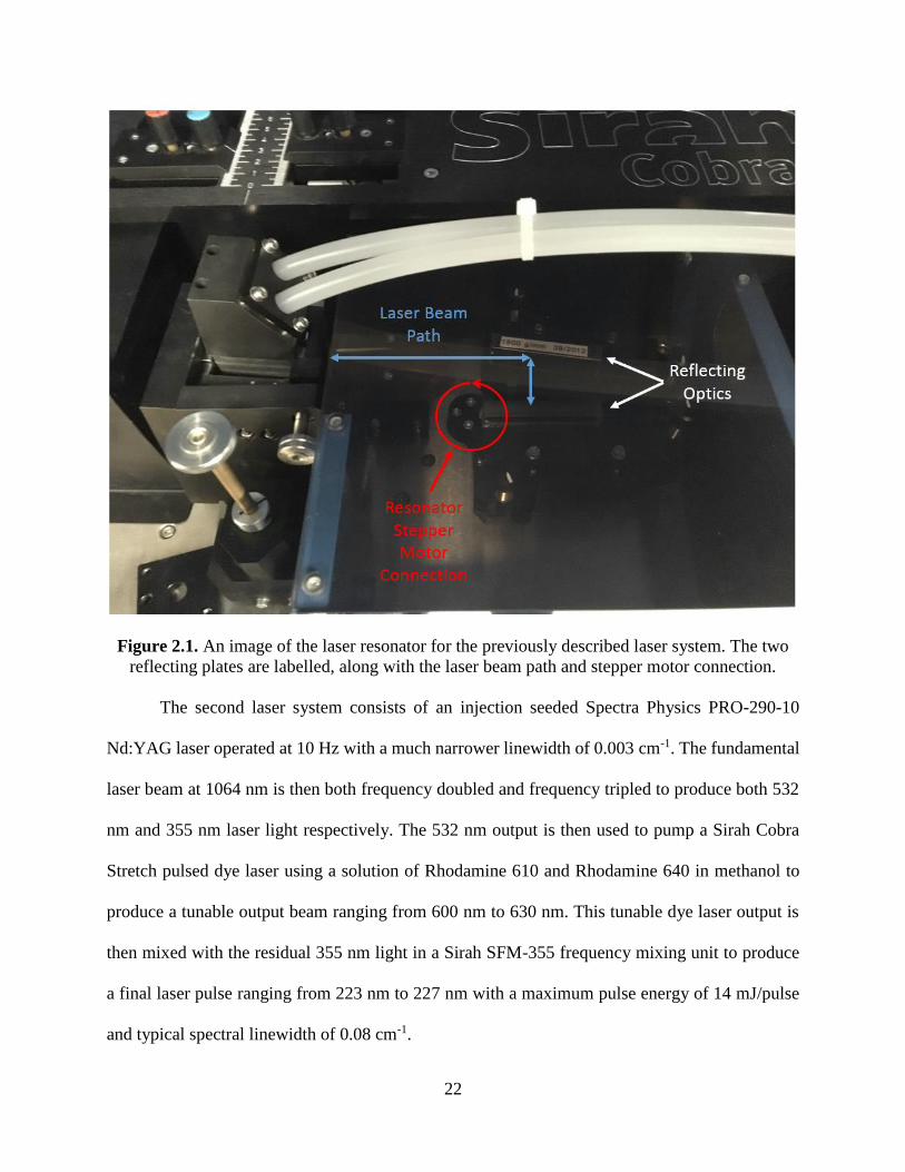
1.2 mJ/pulse. The laser resonator is shown below in Figure 2.1. The stepper motor within the

resonator rotates to change the position of the two reflecting plates, altering the specific

wavelength that is subsequently amplified in the laser resonator.

22

Figure 2.1. An image of the laser resonator for the previously described laser system. The two

reflecting plates are labelled, along with the laser beam path and stepper motor connection.

The second laser system consists of an injection seeded Spectra Physics PRO-290-10

Nd:YAG laser operated at 10 Hz with a much narrower linewidth of 0.003 cm-1. The fundamental

laser beam at 1064 nm is then both frequency doubled and frequency tripled to produce both 532

nm and 355 nm laser light respectively. The 532 nm output is then used to pump a Sirah Cobra

Stretch pulsed dye laser using a solution of Rhodamine 610 and Rhodamine 640 in methanol to

produce a tunable output beam ranging from 600 nm to 630 nm. This tunable dye laser output is

then mixed with the residual 355 nm light in a Sirah SFM-355 frequency mixing unit to produce

a final laser pulse ranging from 223 nm to 227 nm with a maximum pulse energy of 14 mJ/pulse

and typical spectral linewidth of 0.08 cm-1.

23

II.2 Calibration of Laser System

Both previously described laser systems were calibrated with a custom wavelength

scanning program written in Labview. The program functions by initially moving the dye laser

resonator to several wavelength positions and automatically scanning the stepper motor in the

frequency conversion unit while measuring the 226 nm output beam. A Gaussian function is the

least-squares fit to the plot of 226 nm intensity vs. frequency conversion unit motor position. The

frequency conversion unit position that produces maximal signal for this Gaussian fit is then noted,

and a corresponding linear plot of frequency conversion unit vs. laser resonator wavelength is

produced and saved in the laser system’s configuration files. Figure 2.2 below displays both a

sample Gaussian fitting to the 226 nm output intensity vs. frequency conversion unit position and

Figure 2.3 shows a plot of frequency conversion unit position vs. resonator wavelength doubled.

Figure 2.4 shows the BBO crystal, which is tuned to maximize the output of 226 nm light.

Figure 2.2. An example of a Gaussian fitting to a measured intensity peak when scanning the

frequency conversion unit of a laser vs. the produced 226 nm intensity.

24

Figure 2.3. A sample plot of a scan of the frequency conversion unit motor position vs. the

wavelength produced by the laser at the location of maximum signal. For both laser systems

previously described, the best fit function is a first-order polynomial.

Figure 2.4. An image of the BBO contained in the FCU of the laser system. The red arrow

signifies where the stepper motor is changing positions as the motor position is scanned.

II.3 Laser Induced Fluorescence Calibration

An experimental calibration cell was used to calibrate the laser systems to probe excitations

in the NO (X→A) (0,0) band. This involved the slow flow of a low pressure of NO in N2 (< 2 torr)

25

through the cell while the excitation laser was aligned along the axis of the calibration cell. The

laser signal which passed completely through the cell was then scattered off a photodiode and this

signal was used as a timing trigger for a Hamamatsu Type H6780-03 PMT located perpendicular

to the laser axis at the side windows of the slow flow test cell. This cell was also coupled to a

Leybold D65B backing pump and Ruvac WS1001US Roots blower system. This allowed the probe

region of the cell to be refreshed between every laser pulse. A diagram of the test cell setup can be

seen below in Figure 2.5. Clearly labelled are the photodiode, PMT, laser beam path, and flow

inlet and outlet of gas through the cell.

Figure 2.5. A diagram of the calibration cell used for the scanned laser systems.

26

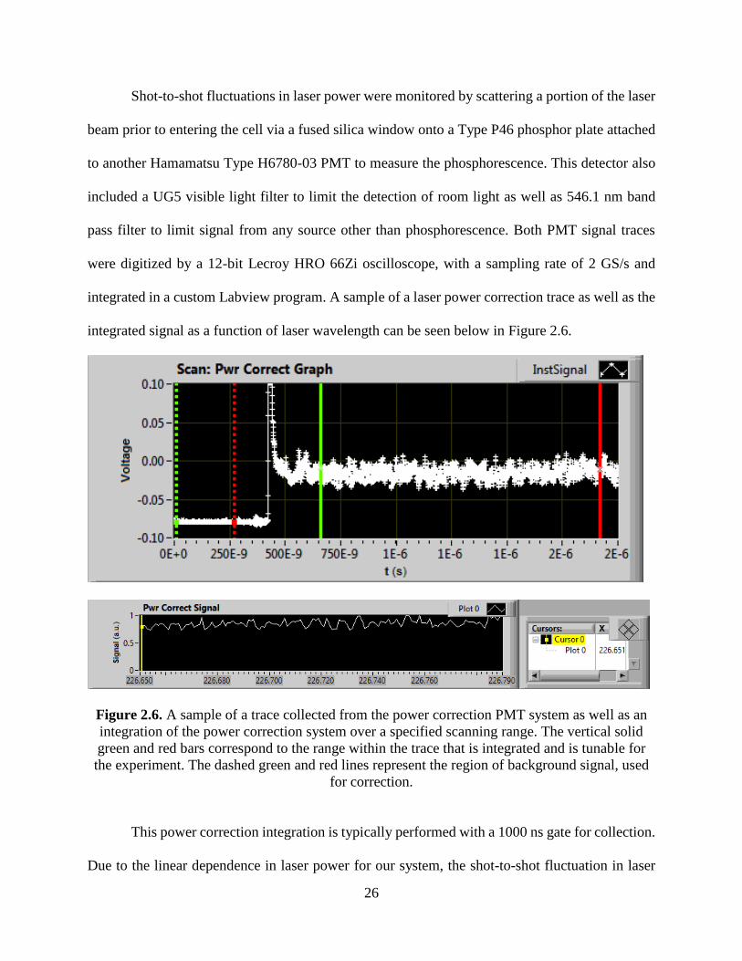
Shot-to-shot fluctuations in laser power were monitored by scattering a portion of the laser

beam prior to entering the cell via a fused silica window onto a Type P46 phosphor plate attached

to another Hamamatsu Type H6780-03 PMT to measure the phosphorescence. This detector also

included a UG5 visible light filter to limit the detection of room light as well as 546.1 nm band

pass filter to limit signal from any source other than phosphorescence. Both PMT signal traces

were digitized by a 12-bit Lecroy HRO 66Zi oscilloscope, with a sampling rate of 2 GS/s and

integrated in a custom Labview program. A sample of a laser power correction trace as well as the

integrated signal as a function of laser wavelength can be seen below in Figure 2.6.

Figure 2.6. A sample of a trace collected from the power correction PMT system as well as an

integration of the power correction system over a specified scanning range. The vertical solid

green and red bars correspond to the range within the trace that is integrated and is tunable for

the experiment. The dashed green and red lines represent the region of background signal, used

for correction.

This power correction integration is typically performed with a 1000 ns gate for collection.

Due to the linear dependence in laser power for our system, the shot-to-shot fluctuation in laser

27

power was corrected by dividing any measured fluorescence signal by this integrated power correct

signal.

To correct for potential wavelength shifts in the laser induced fluorescence of NO from a

prediction produced by the spectral simulation program LIFBASE, 5-10 fluorescence traces are

collected for each laser wavelength position to produce an experimental spectrum across a

wavelength range of interest. A sample generated NO spectrum can be seen below in Figure 2.7,

where peak assignments are specified within the program. With the custom Labview program

previously mentioned, parameters such as step size, shots to average per wavelength and the

wavelength range can be specified. This calibration in the slow flow cell was performed at the start

of each experiment to properly tune the laser to a correct spectral band and peak within a spectral

band.

Figure 2.7. A sample spectrum for NO LIF from LIFBASE. This model is for a temperature of

56 K and line resolution of 0.01 nm. Both of these parameters are tunable within the program.

28

II.4 Detection Systems

Several fluorescence detection systems were utilized in this work, including a combination

of photomultiplier tubes and charge coupled devices. For time-dependent measurement of

fluorescence decays in both room temperature and low temperature experiments, a micro-channel

plate photomultiplier tube (Hamamatsu R5916U-50) was used with a typical operating voltage

ranging from -2.3 to -2.6 kV. The signal produced by this MCP-PMT was digitized by the 12-bit

LeCroy oscilloscope mentioned previously. No wavelength selective filtering was normally

employed on the emission for this system, however a neutral density filter was implemented to

limit the voltage generated by the MCP-PMT while keeping the operating voltage high to preserve

the time-resolution. This MCP-PMT system could also be coupled with a UKA 105 mm F/4.0 UV

lens to further improve signal-to-noise for low fluorescence, high quenching systems. The gating

for all optical and laser systems was controlled by either a BNC 565 or 575 digital delay generator.

For imaging experiments, two different camera systems were employed. An Andor iStar

DH734 ICCD camera was used with the same UKA 105 mm F/4.0 UV lens. This camera system

obtained experimental resolutions of ~0.062 mm/pixel with no pixel binning. This camera system

also allows for integration on the CCD for improved signal-to-noise for individual images. A

custom Labview program was used to both collect and analyze the images from this camera

system. A Princeton Instruments PI-MAX4 ICCD camera was also used in this work, when higher

resolution was required. This camera was fitted with a CERCO 100 mm F/2.8 UV lens with any

number of extension rings to increase magnification to a desired level. This camera system

obtained resolutions of ~0.012 mm/pixel with no pixel binning. The PI-MAX4 camera system

requires proprietary software for the image collection and exported .tif image files were later

29

analyzed in a custom Labview program. Both camera systems were triggered by the previously

mentioned BNC 565 and 575 systems.

II.5 Temperature Analysis Program

The temperature analysis in this work was performed by a custom Labview program and

based on a Boltzmann model for temperature. A Boltzmann distribution calculates the probability

of a certain energy state population as a function of the energy of that state as well as the

temperature of the system. The equation for a Boltzmann distribution is seen below

𝑃𝑛 =𝑔𝑛𝑒

−𝐸𝑛/𝑘𝑇

∑ 𝑔𝑖𝑒−𝐸𝑖/𝑘𝑇𝑁𝑖=1

where Pn is the probability of a molecule existing in a state n, k is the Boltzmann constant (1.38 x

10-23 J/K), T is temperature, gi is the degeneracy of state i, En is the energy of state n, and N is the

number of states of interest. This model can be applied to the relationship between two rotational

energy levels of a molecule by the equation

𝑃1𝑃2=𝑆𝑓,1

𝑆𝑓,2= 𝐶12

(2𝐽1 + 1)

(2𝐽2 + 1)𝑒𝐸2−𝐸1𝑘𝑇

where P1 and P2 are relative populations of the two rotational states, C12 is an experimental fitting

parameter that depends on stimulated absorption coefficients, wavelength dependences in

excitation intensity, the fluorescence quantum yield, and the efficiency of the detector and any

collection optics present, Sf,i is the term for fluorescence signal of state i, as previously described

in Chapter 1, and J1 and J2 are the two rotational states of interest. For determining the temperature

with two rotational populations, the value of C12 is determined by measuring a region of known

temperature for a given experiment. For pulsed supersonic measurements, this was normally done

by measuring the area outside of the gas pulse, where the measured temperature is expected to

30

match the wall temperature. After determining the C12 constant for an experimental setup, two

fluorescence images can be directly compared to determine a temperature map.

For measurements of multiple rotational states (> 2) for determining a temperature, the

equation

𝐸𝐽 = −(ln(𝑃𝐽/(2𝐽 + 1)))𝑘𝑇 + 𝐶

where C is a constant, allows one to solve for temperature by finding the slope of the graph of the

energy of a rotational level vs. the natural log of the measured population at that level. The custom

temperature fitting program utilized in this work for multiple (> 2) rotational population

measurements uses this functional form. For determining the population for a spectral line, a

Gaussian distribution is fit to the rotational peak via least squares fitting. This Gaussian fit is then

integrated to determine the population at that given spectral line. A sample plot of a linear

temperature fitting to six measured rotational populations is seen below in Figure 2.8. While

several J-states can be measured, the automated fitting process has a threshold for the quality of

the fit, where non-Gaussian line shapes are not considered. For this particular example, six total

peaks were within this fitting threshold. The experimental fluorescence spectrum is overlaid in the

figure, with each individual rotational line labelled, with the corresponding data point.

31

Figure 2.8. A sample measurement of measured rotational populations vs. rotational energy. The

linear fit corresponds to a temperature of 92.7 K. The measured fluorescence scan is shown in

the top right corner, and the relevant J-state of each peak and point are labelled.

II.6 Gas Injection System

The substitution of pulse valves for commercially available fuel injectors in pulsed

hypersonic experiments has several benefits; the availability of the components, the durability of

the injectors, and the economic savings when compared to the costs of pulse valves. Previous

studies have substituted fuel injectors for pulse valves in experiments involving naphthalene

fluorescence lifetime measurements [51] as well as measuring the ionization spectrum of NO [52].

Currently a manuscript is in preparation by Prophet, Winner, North, and Sanchez-Gonzalez, which

describes an experimental characterization for these injectors for our pulsed de Laval systems in

this work. This section will briefly highlight key measurements taken from this manuscript.

32

The characterization of commercially available high performance, high impedance, 1600

cc/min fuel injectors (Five-o motorsports, part number 0426US1600) was performed to assess the

fuel injectors as an alternative to pulse valves. This characterization involved the measurement of

opening times, effects of trigger voltage and driver voltage, the reproducibility of the pulses

delivered and the mass flow rates of the pulse valves. A custom made fuel injector driver circuit,

with a TIP121 NPN transistor as the main component used to trigger the injectors, delivered 5 V

adjustable length pulses. This custom circuit was then triggered by a pulse/delay generator (BNC

565), to test for varying pulse lengths and opening times.

Since pulsed gas systems are normally synchronized with other instrumentation for a given

experiment (pulsed lasers, gated collection optics, etc.) the injector response time must be highly

reproducible. The response time is defined as the time delay from the initial trigger signal being

sent to the injector to the time the injector opens. The opening time refers to the time it takes for

the fuel injector to fully open once the solenoid is initially triggered. Both the response time and

the opening times were characterized by triggering the fuel injectors 1 cm away from a fast-

response Kulite XT-190-25A pressure sensor. The rising edge of these pressure traces was fit with

a Gauss error function and a sample plot of measured pressure traces with varying backing

pressures and their comparison to this error function can be seen below in Figure 2.9. The full

width half max of this rising edge was reproducibly found to be 160 ± 20 μs.

33

Figure 2.9. A comparison of experimentally measured time resolved pressure traces

compared to Gauss error function fittings. The experimental data is represented by the dotted

traces, while the fits are the solid colored lines.

Further measurements were made of the dependence on opening time for varying driver voltages

as well as downstream pressure. The opening times were found to increase with increased driver

voltage, with a driver voltage of 9 V corresponding to an opening time of 197 ± 25 μs (with a

backing pressure of 25 psi injecting at atmosphere) and a driver voltage of 16 V corresponding to

an opening time of 77 ± 9 μs. Lower post-injector pressures were found to increase the measured

opening times, with an injector with a 9 V driver pulse at a backing pressure of 25 psi into vacuum

producing an opening time of 420 ± 50 μs. Also of note is that the flow rates across the fuel

injectors was found to be linear with respect to backing pressure, as seen in Figure 2.10 below.

34

Figure 2.10. A measurement of the flow rate dependence on backing pressure. The data is fit

with a least-squares linear function. Error bars are displayed, but error in the flow rate

calculation was found to be < 4% for all backing pressures tested.

35

CHAPTER III

CHARACTERIZATION OF TEMPERATURE DEPENDENT COLLISIONAL QUENCHING

OF NO (A 2Σ+) BY BENZENE AND HEXAFLUOROBENZENE

III.1 Previous LINE Measurements

The temperature dependent collisional quenching rates of NO (A 2Σ+) by benzene and

hexafluorobenzene depend on the number density of the quencher in a particular flow. Thus, if the

quenching cross sections are characterized, a measured fluorescence decay rate can be used to

indirectly solve for the concentration of the quencher in a flow field. This measurement of

quencher concentration is important with respect to the previous studies of Laser Induced Non-

Equilibrium (LINE) performed by West et al. [53]. The authors of this work studied the collisional

energy transfer rates for vibrationally excited benzene molecules with N2 gas, using NO as a tracer

species to monitor temperature. This was performed by flowing room temperature gas mixtures of

benzene, N2, and NO in the slow flow cell previously described in Chapter 2. The gas mixtures

were then perturbed by 193 nm electronic excitation of the benzene present. The excited benzene

undergoes rapid internal conversion followed by intramolecular vibrational redistribution. The

authors then monitored the vibrational to rotational energy transfer between benzene and N2 by

monitoring the temperature of the NO tracer using a 226 nm laser to probe NO (X 2Π1/2) -> NO (A

2Σ+) rotational transitions and measuring the fluorescence emission using an ICCD camera.

This temperature measurement was then compared to temperature rises predicted from a

master equation model. This then allowed the determination of the vibrational relaxation rate for

benzene with N2. This master equation modelling utilized the equation

36

𝑑𝑦(𝐸′, 𝑡)𝑑𝐸′

𝑑𝑡= ∫ [𝑅(𝐸′, 𝐸)𝑑𝐸′𝑋(𝐸, 𝑡)]𝑑𝐸 − ∫ [𝑅(𝐸, 𝐸′)𝑑𝐸′𝑋(𝐸′, 𝑡)]𝑑𝐸

∞

0

∞

0

where X(E’,t)dE’ is the number of molecules with an energy between E’ and E’ + dE’, and R(E,E’)

is the rate coefficient for vibration to rotational/translational collisional energy transfer from an

energy between E’ and E’+dE’ to an energy state with energy between E and E+dE [54, 55]. This

energy transfer rate coefficient can be further expressed by the equation below

𝑅(𝐸, 𝐸′)𝑑𝐸 = 𝜔𝑃(𝐸, 𝐸′)𝑑𝐸

where ω is the collision rate of the system and P(E,E’) is the probability that a molecule with an

energy between E’ and E’+dE’ will undergo a change in energy after a collision to a state with

energy between E and E+dE. Several different functional forms of P(E,E’) have been used in the

past to characterize collisional energy transfer [56-58]. A generalized form of this function is seen

below

𝑃(𝐸, 𝐸′) = 1

𝐶(𝐸′)∑𝑓𝑖𝐸𝑋𝑃 (−(

𝐸′ − 𝐸

𝛼𝑖(𝐸′))

𝛾𝑖

) , 𝐸′ ≥ 𝐸

𝑁

𝑖=1

where C(E’) is a normalization constant, N is the chosen number of exponentials used, fi is the

normalized weight of the exponential functions, αi(E’) is the main fit parameter that is related to

the average amount of energy transferred per collision, and γi is another fit parameter, which for

these studies, was set to 1.

It was found that the experimental data could be accurately modelled with an energy

dependent form of this α(E’) term. More specifically, a functional form of

𝛼(𝐸′) = 𝐶0 + 𝐶1𝐸′

was utilized, where C0 and C1 are fit parameters. This energy dependent functional form was

necessary for fitting the data, due to the curvature of the temperature rise measurements over time.

37

A comparison of master equation simulations using an energy dependent and energy independent

form of α to an experimental temperature rise measurement can be seen below in Figure 3.1.

Figure 3.1. A plot showing an experimental temperature rise at 18 torr compared to an energy

independent model for α and an energy dependent model for α.

The slow flow cell used for these measurements included a N2 window purge line to

prevent benzene molecules travelling down the metal arms of the cell, which could lead to benzene

ablation at the Brewster windows, causing a decrease in the transmittance of the window. This

purge system, coupled with the gas sample injection at the center of the cell led to a gradient of

both benzene and NO concentration in the cell. Due to the usage of an ICCD camera for

fluorescence detection, a large spatial range inside the cell was imaged. The gradient of benzene

in the slow flow cell, coupled with the attenuation of the 193 nm laser beam as benzene was

absorbed across the cell, leads to a gradient of measured temperature rises for each image pair

38

taken. These temperature rises have a dependence on both the local concentration of benzene and

the intensity of 193 nm light on a pixel-by-pixel basis. Pixels were then binned based on similar

temperature rises and thus, multiple temperature rise measurements were performed

simultaneously.

The experimental results were compared to computational simulations performed by Paul

and coworkers [59-61], where chemical dynamic simulations were used to model this experimental

energy transfer data. An important result from this study was the comparison of efficiencies for

different energy transfer processes in this system. The authors found the most efficient process to

be vibrational energy transfer from vibrationally excited benzene to unexcited benzene, with

vibrational to vibrational energy transfer between benzene and N2 being negligible. The slower

rotational-translation heating of the bath was seen for both benzene and N2 and was consistent with

the experimental measurements previously discussed.

Although multiple scales of temperature rises were measured experimentally for these

systems, it is unclear for each pixel grouping whether these differences were due to the local

benzene concentration or laser power. Therefore, it is beneficial to develop a method of

determining a spatially resolved number density of benzene on a pixel-by-pixel basis for these

measurements.

As previously stated in Chapter 1, the absorption of a photon at 226 nm by NO leads to NO

(A 2Σ+), which then has two distinct processes for relaxation to NO (X 2Π1/2); fluorescence and

collisional quenching. The fluorescence process has an intrinsic rate constant, which for NO (A

2Σ+) is 5.1 x 106 s-1 [62]. The quenching rate constant is dependent on the collisional partner, the

number density of the collisional partner, and the local temperature. If the temperature dependence

of the quenching rate constant is well characterized, then the fluorescence decay rate can be used

39

to calculate the number density of a given quenching partner. Thus, the characterization of

temperature dependent collisional quenching of NO (A 2Σ+) by benzene will allow the local

determination of the benzene concentration on a pixel-by-pixel basis for the LINE studies

previously described. These measurements were performed in a similar fashion to previous

temperature dependent quenching rate constant measurements for NO (A 2Σ+) with quenching

partners O2 and N2 by Sanchez-Gonzalez and coworkers [63]. The authors of this study found that

the quenching behavior at low temperature (34 K – 109 K) followed an inverse power law model,

where a monotonic increase in collisional quenching was observed with a decrease in temperature.

III.2 Experimental Method

The determination of thermally averaged collisional quenching cross sections for NO (A

2Σ+) by benzene and hexafluorobenzene was performed in the slow flow cell and the pulsed

hypersonic test cell previously described in Chapter 2. All equipment listed in this section has been

described in Chapter 2, unless stated otherwise. The fluorescence decay rate of NO (A 2Σ+) was

measured for varying concentrations of benzene and hexafluorobenzene at a stable temperature

and pressure. The slow flow cell was kept at a constant temperature of 300 K via heating tape

wrapped around the cell, with an attached thermocouple to monitor the real time temperature at

the location of the gas inlet. The cell was evacuated using a Ruvac WS10001US Roots blower

backed by a Leybold D65B pump. The flow of the prepared gas sample into the test cell was

controlled by the mass flow controller system previously described, and operated in a constant

flow mode. The pressures within in the cell as well as the region behind the injection section were

monitored with two pressure transducers. The cell pressure was nominally maintained between 5

and 6 torr for all tested concentrations of quenchers. There was a slight variance in NO number

40

density in the cell, with a dependence on the collisional quencher concentration. This is due to the

method of gas sample preparation, which is discussed below.

The measurement of collisional quenching at lower temperatures (<200 K) was performed

in the pulsed hypersonic test cell previously described. By utilizing several different de Laval

nozzles representing a range of Mach numbers, as well as external heating of the pre-expansion

region of the cell, a wide range of operating temperatures were obtained post-expansion. This

controlled heating of the pre-expansion region was performed with heating tape and an attached

thermocouple to monitor temperature, similar to the heating control used in the slow flow cell.

Pressure matching of the nozzle during operation was performed with the two fast response

pressure transducers previously described.

The flow temperature for measurements in both the slow flow cell as well as the pulsed

hypersonic test cell was monitored by probing the Q2 + R12 and P2 + Q12 bands in the NO X -> A

transition. Ten rotational state populations were measured and the flow temperature was calculated

by using a Boltzmann plot of the relative rotational populations determined by Gaussian fitting of

the rotational peaks. A sample spectrum is shown below in Figure 3.2, with the ten measured peaks

labelled.

41

Figure 3.2. Experimental LIF spectrum for NO (X->A). The bands measured were Q2 + R12 and

P2 + Q12 and the specific j-states used for temperature fitting are labelled. This fluorescence scan

is for a sample at approximately 300 K.

The gas samples for both test cells were prepared by initially combining a fixed ratio of

5% NO/N2 with 99.995% N2 with the mass flow controller setup previously described. This

mixture was then passed through a high pressure bubbler containing either 99.8% anhydrous

benzene or 99% hexafluorobenzene. This bubbler system was kept at a near constant temperature

(~286 K) with a custom built water cooling stainless steel coil system to maintain a constant vapor

pressure of benzene or hexafluorobenzene. To vary the percentage of benzene or

hexafluorobenzene in the prepared gas sample, the total pressure introduced into the bubbler

system was varied. Since the vapor pressure of the quenching species remains constant for this

process, the total number density of the quenching species present in the test cell can be determined

42

by using the ratio of introduced pressure into the bubbler to the vapor pressure of the quencher, as

well as the temperature and total pressure inside of the flow cell, for both the slow flow cell as

well as the pulsed hypersonic test cell.

The control of benzene concentration with this bubbler system was validated by UV-Vis

absorption measurements in the same slow flow cell previously used for the 300 K measurements

of quenching. The UV-Vis light source was sent through the sides of the cell and the spectrometer

was aligned at the opposite window of the cell. This was done to prevent the gradient of benzene

along the Brewster angle window arms from affecting the absorbance measurement. In these

absorption measurements, the same experimental conditions were maintained for the mixing

region in both the slow flow room temperature measurements as well as the low temperature pulsed

hypersonic measurements. The absorption of benzene was measured from 225 nm to 265 nm by

an Ocean Optics USB2000+UV-VIS spectrometer with a collection time of 350 ms and 100

spectra averaged. This spectral range includes the S0 (1A1g) -> S1 (

1B2u) electronic transition of

benzene, and the peaks in this region are a result of the rovibrational structure from this transition

[64]. The measured absorbance spectrum was then compared to one previously determined by

Olive [65, 66] and the comparison can be seen below in Figure 3.3. Since the experimentally

measured absorbance spectrum determined in this work was a lower spectral resolution than the

spectrum reported by Olive et al., the literature spectrum was Gaussian blurred to match the

resolution of our reported spectrum. The original absorbance spectrum compared to the Gaussian

blurred form can be seen in Figure 3.4.

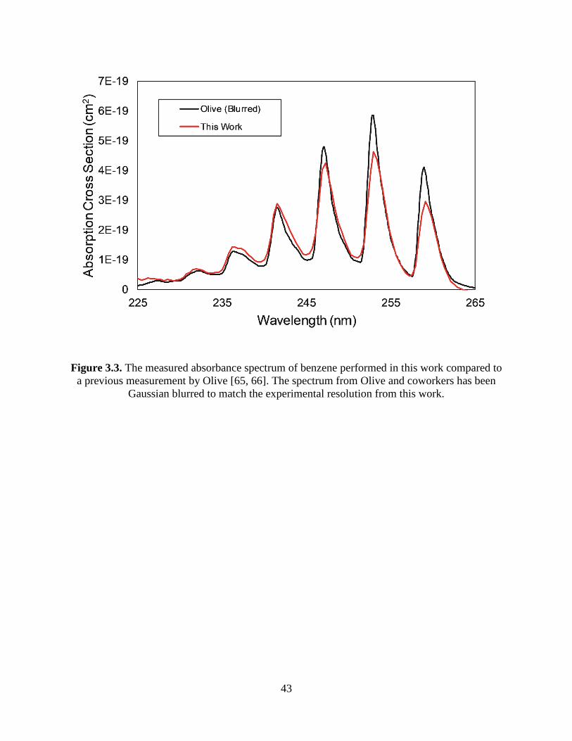
43

Figure 3.3. The measured absorbance spectrum of benzene performed in this work compared to

a previous measurement by Olive [65, 66]. The spectrum from Olive and coworkers has been

Gaussian blurred to match the experimental resolution from this work.

44

Figure 3.4. A comparison of the spectrum from Olive [65, 66] to the Gaussian blurred version of

the spectrum used for comparison to the experimental measurements taken in this work.

The absorption line at 238.3 nm was then used to obtain a Beer’s law plot (seen below in

Figure 3.5) by varying the concentration of benzene in the sample gas and monitoring the relative

absorbance. This feature was chosen to avoid issues of saturation at higher wavelength peaks,

which is the cause of deviation of the absorption spectrum measured in this work compared to that

from the literature past 245 nm in Figure 3.3. This plot is seen below, with a linear fit through the

origin. Based on the slope of this linear fit, the absorption cross section was determined to be 1.21

± 0.07 x 10-19 cm2. This is in excellent agreement with the previously measured absorption cross

section of 1.15 x 10-19 cm2 at the same wavelength [65, 66]. In addition to this determined cross

section, the concentration of benzene was found to be invariant with respect to the overall flow

rate through the bubbler system.

45

Figure 3.5. A Beer’s law plot of benzene absorption at 238.3 nm vs. benzene concentration. The

linear fit has an R2 = 0.9927 with the experimental data and the fit is forced through the origin.

These UV-Vis absorption measurements clearly show the efficacy of our benzene and

hexafluorobenzene bubbler system for the precise control of collisional quencher concentrations.

The laser induced fluorescence decay rates for our prepared gas samples were measured

by probing the R12 + Q2 band at j = 6.5. Collisional quenching rates have been previously shown

to be independent of measured rotational state for NO (A 2Σ+) for a variety of quenchers [67-70].

The j = 6.5 rotational state was chosen due to the fluorescence signal being relatively high intensity

across the entire range of temperatures in this work. The total laser pulse energy of the 226 nm

beam was measured to be approximately 300 μJ/pulse. Under these conditions, the absorption of

NO is calculated to be approximately 0.15%. This relatively low amount of absorbance is

important for limiting undesired photophysics and potential multi-photon effects, since the

residence time in the slow flow cell was slightly greater than 1 s at the experimental flow rates,

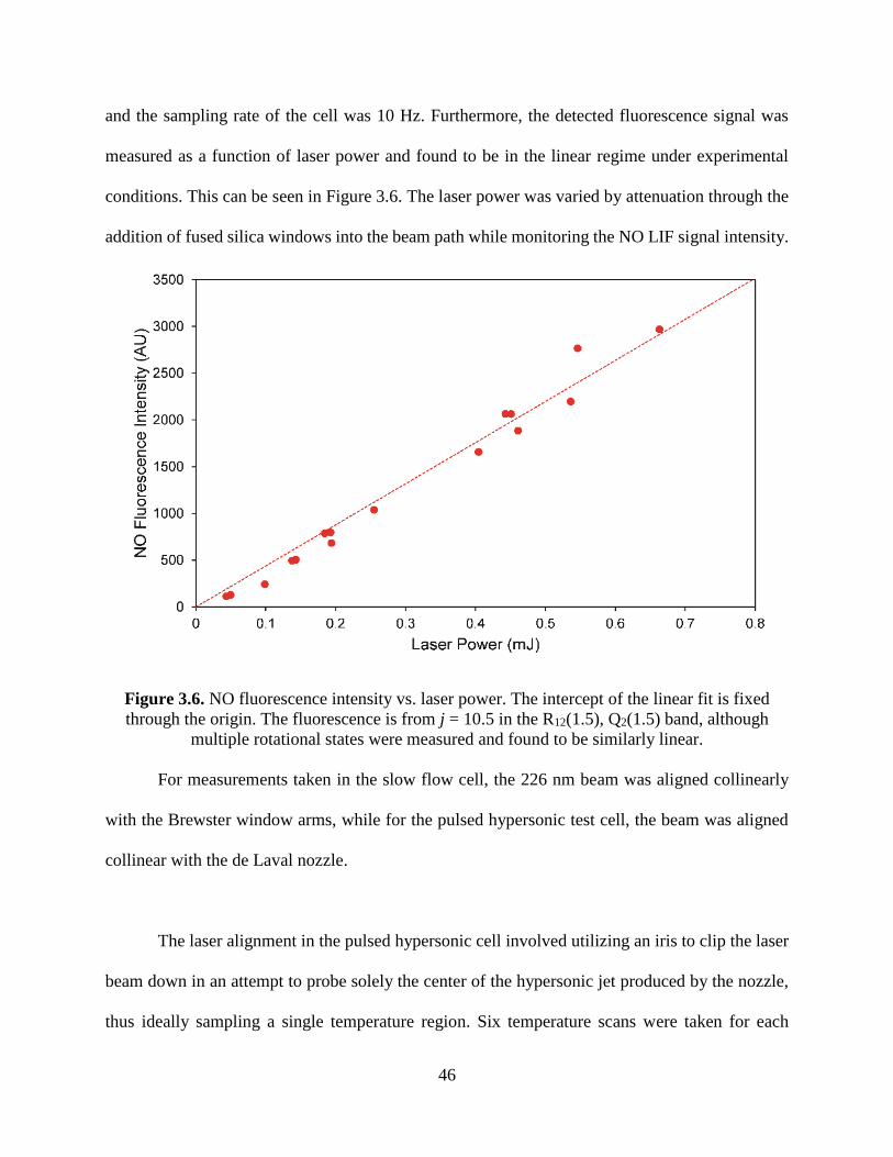
46

and the sampling rate of the cell was 10 Hz. Furthermore, the detected fluorescence signal was

measured as a function of laser power and found to be in the linear regime under experimental

conditions. This can be seen in Figure 3.6. The laser power was varied by attenuation through the

addition of fused silica windows into the beam path while monitoring the NO LIF signal intensity.

Figure 3.6. NO fluorescence intensity vs. laser power. The intercept of the linear fit is fixed

through the origin. The fluorescence is from j = 10.5 in the R12(1.5), Q2(1.5) band, although

multiple rotational states were measured and found to be similarly linear.

For measurements taken in the slow flow cell, the 226 nm beam was aligned collinearly

with the Brewster window arms, while for the pulsed hypersonic test cell, the beam was aligned

collinear with the de Laval nozzle.

The laser alignment in the pulsed hypersonic cell involved utilizing an iris to clip the laser

beam down in an attempt to probe solely the center of the hypersonic jet produced by the nozzle,

thus ideally sampling a single temperature region. Six temperature scans were taken for each

47

benzene and hexafluorobenzene concentration measured for each experimental combination of de

Laval nozzle and heating of the pre-expansion region to determine the stability of this temperature

sampling method. The temperature was measured with < 6% variance for all samples considered

for individual experimental setups.

The fluorescence signals were collected on an MCP-PMT previously described, with

operating voltages ranging from -2.3 to -2.6 kV. The MCP-PMT was gated with a delay of 50 ns

after the triggering of the laser system in an attempt to limit scattering signal, which is on the

timescale of the laser line width (approximately 10 ns). A collection time of 1000 ns was utilized

to allow a full collection of fluorescence signal as well as collection of background noise after the

fluorescence decay, with the intrinsic fluorescence decay lifetime of NO X -> A being

approximately 192 ns [62]. No wavelength dependent filtering was performed on the emission

prior to collection and thus the entire vibrational progression was collected. Each measured

fluorescence decay was corrected by subtracting traces taken with the laser system off resonance,

to correct for background issues. A total amount of 500 fluorescence decays were sampled for each

concentration of benzene and hexafluorobenzene tested, as well as 500 off resonant traces.

III.3 Results and Analysis

After the initial formation of NO (A 2Σ+) by our 226 nm laser system, the measured

fluorescence decay is a result of the combination of spontaneous emission and quenching:

NO (A 2Σ+) 𝑘𝑓→ NO (X 2Π1/2) + hν

NO (A 2Σ+) + M 𝑘𝑞,𝑀→ NO (X 2Π1/2) + M

where kf is the rate constant for the intrinsic rate of fluorescence of NO (A), M is the specific

collisional quencher of interest, and kq,M is the rate constant for collisional quenching by collision

48

partner M. To solve for the temperature dependent collisional quenching rate constants, each decay

was linearly fit to the integrated rate law:

ln(𝐼(𝑡) − 𝐼𝑂𝑅) = −(𝑘𝑡𝑜𝑡𝑎𝑙) 𝑡 = −(𝑘𝑓 +∑𝑘𝑞,𝑀[𝑀])

𝑀

𝑡

where I(t) is the fluorescence intensity at time t, IOR is the measured signal with the 226 nm laser

off resonance, and [M] is the total number density of the quenching species of interest, where each

quencher present for a given experiment has a unique quenching rate constant. Sample decays can

be seen below in Figure 3.7, where the three decays represent three different experimental

concentrations of benzene. The fluorescence decays displayed excellent linearity over

approximately two orders of magnitude. This would indicate pseudo first order kinetics with

respect to benzene concentration. All decay fitting was performed 15 ns after the initial laser

excitation signal to limit effects due to scattering.

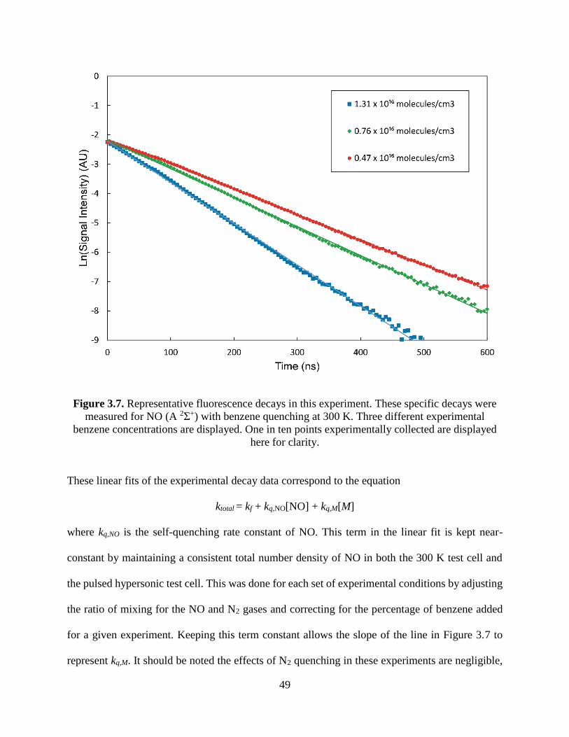
49

Figure 3.7. Representative fluorescence decays in this experiment. These specific decays were

measured for NO (A 2Σ+) with benzene quenching at 300 K. Three different experimental

benzene concentrations are displayed. One in ten points experimentally collected are displayed

here for clarity.

These linear fits of the experimental decay data correspond to the equation

ktotal = kf + kq,NO[NO] + kq,M[M]

where kq,NO is the self-quenching rate constant of NO. This term in the linear fit is kept near-

constant by maintaining a consistent total number density of NO in both the 300 K test cell and

the pulsed hypersonic test cell. This was done for each set of experimental conditions by adjusting

the ratio of mixing for the NO and N2 gases and correcting for the percentage of benzene added

for a given experiment. Keeping this term constant allows the slope of the line in Figure 3.7 to

represent kq,M. It should be noted the effects of N2 quenching in these experiments are negligible,

50

since the cross section of N2 quenching NO (A 2Σ+) is approximately 5000 smaller than the self-

quenching cross section of NO for both the 300 K experiments as well measurements taken at

lower temperature [63].

For the measurements at 300 K in the slow flow test cell, the total number density was

determined by measuring the pressure within the cell using the previously described pressure

transducer and the spectroscopically determined temperature. For the measurements performed at

low temperature in the pulsed hypersonic test cell, the fast response pressure sensor previously

mentioned was used to determine the impact pressure at the nozzle exit. This impact pressure was

then converted to the static pressure of the flow via the equations of isentropic flow of a perfect

gas through a converging-diverging nozzle and accounting for the Mach number of a particular de

Laval nozzle.

To determine the predicted contribution of NO self-quenching for each set of experimental

conditions, the temperature dependent self-quenching rate constant model reported by Sanchez-

Gonzalez et al. [63] were calculated for each experiment, where the equation

𝜎𝑁𝑂 = 40.7(300

𝑇)0.22 + 25.7𝑒

−1380𝑇⁄

was utilized for each data set collected at a specific temperature. These calculated self-quenching

cross sections were used to predict the y-intercepts of the plots of ktotal vs. benzene number density,

as seen below in Figures 3.8 – 3.11.

51

Figure 3.8. A plot of total measured decay rate vs. quencher number density for experimental

measurements at 300 K. The black data is for benzene and the red is for hexafluorobenzene.

52



53



54


measurements at 177 K for benzene and 155 K for hexafluorobenzene. The black data is for

benzene and the red is for hexafluorobenzene.

A measurement of NO self-quenching was initially performed at 300 K to test the efficacy

of our experimental setup and data analysis. The self-quenching rates of NO have been studied

extensively. Our measured self-quenching NO collisional cross section was determined to be 38.5

± 1.3 Å2, which is well within the range of existing literature values of 37-41 Å2 [63, 71-79].

Using the slopes of Figures 3.8 – 3.11, the values of kq,M(T) were determined for each

experiment at a given temperature and collisional quencher. From this value, a collisional

quenching cross section can be determined. This removes the temperature dependence of the

average velocity of the gas molecules in the experiment from the overall temperature dependence

55

of the quenching behavior. This allows for a better comparison to models of collisional quenching.

The quenching cross sections measured in this work were calculated by using the equation

< 𝜎𝑞,𝑀 > = 𝑘𝑞,𝑀√𝜋𝜇𝑁𝑂,𝑀8𝑘𝐵𝑇

where μNO,M is the reduced mass of the quenching partner and NO, kB is the Boltzmann’s constant,

and T is temperature. The values for the quenching cross section for all previously listed

experimental conditions were tabulated and can be seen in Table 3.1 below.

Table 3.1. This table is a summary of the calculated quenching cross sections measured in this

work. The error bars are a result of 2σ error.

Quenching

Species

σ (Å2) at

300 K

σ (Å2) at

130 K

σ (Å2) at

145 K

σ (Å2) at

155 K

σ (Å2) at

177 K

C6H6 147 ± 9 186 ± 10 188 ± 8 NA 175 ± 8

C6F6 133 ± 7 168 ± 13 172 ± 8 167 ± 10 NA

The commonly invoked harpoon mechanism has been used in the past to explain the

collisional quenching of NO (A 2Σ+) by CCl4, CF2Cl2, CH3CCl3, SF6, CF4, CF3Cl, O2, NO, N2, and

SO2 [74, 80]. This mechanism of collisional energy transfer involves an initial step of an electron

transfer from the electronically excited NO to the quenching partner via a curve cross to the ionic

NO+-Q- energy potential and then a subsequent second curve crossing down to the NO (X 2Π1/2)

state, thus resulting in the electronic relaxation of the electronically excited NO. Due to the initial

step involving the transfer of an electron, this step relies on the electron affinity of the quenching

partner being sufficiently high enough to allow the transfer from NO. This is considered to require

an electron affinity larger than -1.0 eV [81]. This mechanism also predicts the quenching

56

characteristics of different molecules to scale with their relative electron affinity. This behavior

can be seen below in Figure 3.12.

Figure 3.12. A plot of experimentally determined quenching cross section vs. the electron

affinity of the quenching partner for NO (A 2Σ+) quenching.

It is apparent in Figure 3.12 that benzene seems to violate the predictions from the harpoon

model. Benzene, with an electron affinity of -1.5 eV [82], is not predicted to be an effective

quencher of NO (A) in the harpoon model. Thus, there must be some other mechanism occurring

for the relatively efficient quenching measured for benzene.

Previous studies have found that the preparation of NO (A 2Σ+) in the presence of ethene

and acetylene has led to products similar to those produced from direct excitation of these

hydrocarbons [83]. This phenomenon is thought to occur through near resonant electronic energy

transfer from the electronically excited NO to the A-states of the hydrocarbons. Furthermore, the

quenching behavior of benzene, toluene, ethene, acetylene, and ammonia do not match the

57

behavior predicted by the harpoon mechanism [74, 81]. All of these molecules would be predicted

to have a negligible quenching cross section due to their electron affinity, as is seen with the

quenching behavior of methane, ethane, and propane. Also for these quenchers with relatively low

electron affinity, the quenching cross section is predicted to increase with temperature, due to the

large energy barrier associated with the harpoon model [84]. Due to the fact that these five

quenchers do not follow the predictions of the harpoon mechanism, and since these quenchers all

have excited electronic states lower in energy than that of NO (A 2Σ+), it is believed that the

quenching mechanism for these systems involves a near resonance electronic energy transfer.

Near resonant electronic energy transfer for these five molecules involves the efficient

transfer of the electronic energy of NO (A 2Σ+) to the rotational and vibrational energy levels of

an excited electronic state in the quencher [85-92]. This process converts a fraction of the energy

from the electronically excited state of NO to electronic excitation in the quenching partner [93].

The rate of this type of energy transfer process is proportional to the electronic coupling between

NO (A 2Σ+) and the acceptor molecule. Both benzene and hexafluorobenzene have A-state energies

lower than that of NO [94, 95], however the benzene A-state energy is slightly closer to that of

NO than the A-state energy of hexafluorobenzene. Therefore, the near resonant electronic energy

transfer model would predict a slightly higher quenching cross section for benzene than

hexafluorobenzene, which matches our experimental measurements for all temperatures. Also of

note is this comparison being contrary to predictions made by the harpoon mechanism, where the

quenching cross section of hexafluorobenzene would be predicted to be significantly larger than

that of benzene due to the much higher electron affinity.

A factor in resonant energy transfer is the capture cross section of the donor with the

quencher. For the determination of a capture cross section, dipole-dipole forces, dipole-induced

58

dipole, and dispersion forces were considered. The potential energy for a dipole-dipole interaction

is

𝑉(𝑟) = −2

3 𝜇12𝜇22

𝑘𝐵𝑇𝑟6

where μi is the dipole constant of molecule i [96], kB is the Boltzmann constant, T is temperature,

and r is the intermolecular distance. The potential for a dipole-induced dipole interaction is

𝑉(𝑟) = −(𝜇1

2𝛼2 + 𝜇22𝛼1)

𝑟6

where αi is the polarizability of molecule i [96]. Lastly, the potential for a dispersion interaction

between molecules is

𝑉(𝑟) = −3𝐼1𝐼2𝛼1𝛼22(𝐼1 + 𝐼2)𝑟6

where Ii is the ionization potential of molecule i [96]. So, when including these three intermolecular

forces, the total potential of the system is

𝑉(𝑟) = −1

𝑟6 (2

3 𝜇12𝜇22

𝑘𝐵𝑇+ 𝜇1

2𝛼2 + 𝜇22𝛼1 +

3𝐼1𝐼2𝛼1𝛼22(𝐼1 + 𝐼2)

)

For determining a capture cross section, the total energy of the system is

𝐸 = 𝜇𝑣2

2= 1

2𝜇(𝑑𝑟

𝑑𝑡)2 +

(𝜇𝑏𝑣)2

2𝜇𝑟2+ 𝑉(𝑟)

where v is the relative velocity of the two molecules, μ is the reduced mass of the two molecules,

and b is the impact parameter of the interaction. Since this is an orbiting collision, 𝑑𝑟

𝑑𝑡= 0.

Observing the form of V(r), a second substitution of

𝑉(𝑟) = −𝑎

𝑟𝑠

can be made into the equation for E, as well as remembering that at the capture cross section,

59

𝑑𝐸

𝑑𝑟= 0

which then gives the generic solution for the cross section

𝜎 = 𝜋𝑏2 = 𝜋 (𝑎(𝑠 − 2)

𝜇𝑣2)

2𝑠

(𝑠

𝑠 − 2)

The experimental quenching cross sections of several molecules compared to their

calculated capture cross sections are seen in Figure 3.13 below. There is a weak positive correlation

evident in the results, which is to be expected of the near resonant electronic energy transfer

mechanism. This also predicts a temperature dependence of T-1/3 for the quenching cross section

of benzene and hexafluorobenzene. It should be noted that dipole moments, polarizability values,

and ionization potentials for the ground state of NO were used, since A-state values are currently

unknown.

60

Figure 3.13. A plot of experimentally measured quenching cross sections for molecules expected

to undergo the resonant energy transfer mechanism for quenching vs. calculated capture cross

sections.

A plot of collisional quenching cross section vs. temperature can be seen below in Figure

3.14. The dotted lines in this figure are a result of least squares fitting the data sets to the function

𝜎 = 𝐴 ∗ 𝑇𝐵

where A and B are fitting coefficients to model the temperature dependence predicted by the

capture cross section model. The least squares fit corresponds to A = 842, B = -0.31 for benzene

and A = 803, B = -0.32 for hexafluorobenzene. These experimentally determined B-values appear

to indicate that the temperature predictions of the capture cross section model are valid, where the

model predicts a B-value of -1/3.

61

Figure 3.14. A plot of collisional quenching cross section vs. temperature for the experiments

performed in this work. The black circles represent benzene measurements and the blue squares

represent hexafluorobenzene measurements. The dotted lines correspond to the least squares

fitting of the function σ = A*TB.

Another effect that is known to be correlated with near resonance electronic energy transfer

is the overlap between the donator emission spectrum and the quencher absorption spectrum [93].

To see this impact, an overlap integration was performed for several quenchers thought to undergo

resonant energy transfer with the A-state of NO. These values were determined using the equation

Overlap = ∑ 𝜑𝑁𝑂 𝑒𝑚𝑖𝑠𝑠𝑖𝑜𝑛𝜑𝑄 𝑎𝑏𝑠𝑜𝑟𝑝𝑡𝑖𝑜𝑛𝑑𝜏

40,000

𝑖= 0

62

where 𝜑𝑁𝑂 𝑒𝑚𝑖𝑠𝑠𝑖𝑜𝑛 is the emission spectrum of the NO A-state, 𝜑𝑄 𝑎𝑏𝑠𝑜𝑟𝑝𝑡𝑖𝑜𝑛 is the absorption

spectrum of quencher Q, and 𝑑𝜏 = 0.001 nm is the step size for the summation. The spectral range

of this calculation was from 225 nm to 265 nm. Absorption data was used for benzene [65], C6F6

[97], NH3 [98], C2H2 [99], toluene [100], CF3I [101], CH3I [102], and SO2 [65]. The NO emission

spectrum was obtained through a simulation in LIFBASE [103, 104]. The results are seen below

in Figure 3.15. Although there is not a monotonic trend in this data, there appears to be a positive

correlation between the spectral overlap and the quenching cross section, as would be expected

from resonant energy transfer.

Figure 3.15. A plot of experimentally determined quenching cross sections with NO (A 2Σ+) vs.

the integrated spectral overlap between the emission spectrum of NO (A 2Σ+) and the absorption

spectrum of the quencher.

63

III.4 Conclusion

In conclusion, the temperature dependent collisional quenching cross sections of NO (A

2Σ+) by benzene and hexafluorobenzene were measured for temperatures ranging from 130 K to

300 K via time resolved fluorescence measurements. The high quenching of benzene violates

predictions made by the harpoon mechanism, where the quenching cross section of a species is

expected to track with its electron affinity. The large cross section for benzene is proposed to arise

from a near resonant electronic energy transfer mechanism, where the electronic excitation of NO

(A 2Σ+) is transferred to the slightly lower in energy A-state of the benzene. This mechanism has

a predicted temperature dependence of T-1/3, since the quenching cross section is expected to be

proportional to the probability of forming an orbiting complex, also known as a capture cross

section, which mainly depends on dispersion forces for the benzene system. This current

temperature dependent quenching model is lacking high temperature (> 300 K) measurements and

thus it would be beneficial in the future to test if this predicted temperature dependence is true at

higher temperatures. It could also prove insightful to test the temperature dependence of the other

quenchers listed in this work expected to undergo the resonant energy transfer mechanism, since

quenchers with a non-zero dipole are predicted to follow a different temperature dependence of T-

2/3.

64

CHAPTER IV

A COMPREHENSIVE ANALYSIS OF THE APPLICABILITY OF THE INVISIBLE INK

VENOM METHOD

IV.1 Introduction

The vibrationally excited nitric oxide monitoring (VENOM) technique involves a

combination of PLIF and MTV measurements utilizing NO as a tracer species, as previously

discussed in chapter 1. To briefly summarize here, this technique involves the initial generation of

a grid of vibrationally excited NO, which is subsequently probed with a planar laser sheet. A cross-

correlation method can then be used to determine a mapping of flow velocity. A second planar

sheet tuned to a distinct rotational state of the vibrationally excited NO is then compared to the

initial “read” sheet via image dewarping, utilizing the measured velocity map. This then allows a

PLIF measurement of the temperature of the flow field in a single-shot correlated manner with the

velocity of the flow. A timing diagram of a typical experiment can be seen below in Figure 4.1. A

typical value of τ1 can range from 500 ns to 2000 ns and the optimal tuning is dependent on the

velocimetry of the flow field. A typical value of τ2 is 400 ns and is kept minimally small to reduce

displacement between the subsequent “read” laser sheets. This time delay is necessary to avoid

measuring fluorescence signal from the first “read” laser sheet with the second camera gate.

65

Figure 4.1. A typical timing diagram of a VENOM measurement.

Past methods of generating vibrationally excited NO involved NO2 photodissociation, as

previously mentioned in chapter 1. To summarize, this involved the photodissociation of NO2 at

335 nm, creating approximately 40% NO (X, v=1). This photodissociation process also imparted

a large thermal perturbation to a flow field [4]. To limit potential thermal perturbations of the

VENOM method, the “invisible ink” variant has recently been developed. This method of

vibrational excitation of NO involves the electronic excitation NO (X 2Π) to (A 2Σ+) at 226 nm.

This is then followed by both spontaneous emission and collisional quenching, resulting in

relaxation to the ground electronic state while also populating several vibrationally excited states.

A energy level diagram of the invisible ink VENOM method can be seen below in Figure 4.2.

This method has been shown to reduce the overall thermal perturbation of a flow field when

utilizing the VENOM method [5]. However, there are still outstanding questions pertaining to the

applicability of this method in more challenging flow facilities, specifically pressure, high

temperature, and air containing flow fields, which could present a challenge.

66

Figure 4.2. An energy level diagram of the invisible ink VENOM method.

For high pressure flow fields, the ratio of collisional quenching to fluorescence is expected

to rise. This will lead to a decrease in detected NO fluorescence signal, with NO lifetimes reaching

levels comparable to laser time widths (~10 ns). Further complicating this issue are air containing

flows, where molecular oxygen is a considerably more efficient quencher of NO (A 2Σ+) than N2

[63]. Lastly, high temperature flow fields may contain several different describable flow

temperatures, with rotational/translational temperatures cooling much faster (< 10 collisions) than

vibrational temperatures (>103 collisions). These effects will impact the lifetimes of the

vibrationally excited NO prepared in these flows, and could impact the efficacy of the VENOM

method for high temperature flows.

In this chapter, the predicted performance of the “invisible ink” VENOM method will be discussed

for three distinct flow facilities found at the National Aerothermochemistry Lab (NAL) at Texas

A&M University. This analysis is performed with a custom kinetics code. This code involves the

initial prediction of generated vibrational, rotational, and translational excitation by the 226 nm

67

laser system in the “write” step of the “invisible ink” VENOM method. This involves a prior

probability calculation to model energy populations due to collisional quenching and a Franck-

Condon calculation for populations due to fluorescence. The code then involves a subsequent

kinetics calculation to further monitor both the rotational/translational rethermalization and the

subsequent, much slower, vibrational rethermalization. This kinetics calculation is performed with

forced harmonic oscillator rate constants, which will be discussed in some detail for their

applicability in these types of experimental systems.

IV.2 Model Description

IV.2.1 Initial Generation of Vibrational/Rotational/Translational Excitation in NO

As stated above, the “invisible ink” method involves the initial excitation of NO (X 2Π) to NO

(A 2Σ+) at 226 nm. This electronic excitation is then followed by two relaxation pathways;

spontaneous emission and collisional quenching. These two pathways produce distinct energy

distributions in both NO as well as the collisional quencher, and thus the initial vibrational

distribution generated by the “invisible ink” method is dependent on the ratio of collisional

quenching to fluorescence. For this work, the ratio of quenching to fluorescence was calculated

via experimentally determined temperature dependent quenching cross sections [63]. The

calculated rate of quenching from these cross sections is then compared to the intrinsic rate of

fluorescence for NO (A 2Σ+) to produce a weighing factor for the energy distribution due to

collisional quenching and the energy distribution due to fluorescence.

The energy distribution resulting from fluorescence is generated from a Franck-Condon

calculation. This calculation is based on the principle that for an electronic transition due to

fluorescence, the change from initial vibrational state to the final vibrational state is dependent on

68

the overlap of the two vibrational wavefunctions. For rotational and translation excitation due to

fluorescence, selection rules limit transitions to Δj = ± 1, and rotational/translation excitation is

considered negligible for this pathway.

For the fraction of NO (A 2Σ+) that undergoes quenching, a prior probability model using

a rigid rotor harmonic oscillator approximation (RRHO) was implemented for the diatomic species

present (NO, N2 and O2) [105-107]. This model is called a prior probability model because it is a

purely statistical prediction made prior to any outside perturbations or forcing behaviors. The

general formula for a prior function is

𝜌0(𝑎𝑖; 𝐸) =𝑔(𝑎𝑖)[𝐸 − 𝜀(𝑎𝑖)]

1/2

∑ 𝑔(𝑎𝑘)[𝐸 − 𝜀(𝑎𝑘)]1/2𝑛𝑘=1

(Eq. 4.1)

where ρ0 is the probability of a particular energy mode ai, E is the total energy of the system (i. e.

the 226nm excitation photon), g(ai) is the degeneracy of mode ai, and ε(ai) is the energy of mode

ai. For a diatomic-diatomic collision, there are 5 energy modes; two vibrational modes, two

rotational modes, and one translational mode. The energy of a vibration is defined by the harmonic

oscillator energy

𝐸𝑣 = (𝑣 +1

2)𝜈𝑒

(Eq. 4.2)

where νe is the fundamental vibrational frequency for the particular diatomic and v is the

vibrational quantum state of interest. The energy of the rotation of a diatomic with a rigid rotor

approximation is defined as

𝐸𝑗 = 𝑗(𝑗 + 1)𝛽𝑒 (Eq. 4.3)

69

where βe is the rotational constant of the particular diatomic molecule and j is the rotational

quantum state of interest. Using these defined energy values, the denominator of equation 4.1

becomes

𝐷 =∑∑∑∑(2𝑗𝑁𝑂 + 1)(2𝑗𝑄 + 1)[𝐸 − 𝐸𝑣,𝑁𝑂 − 𝐸𝑣,𝑄 − 𝐸𝑗,𝑁𝑂 − 𝐸𝑗,𝑄]1/2

𝑗𝑄𝑗𝑁𝑂𝑣𝑄𝑣𝑁𝑂

where jNO and jQ are the rotational quantum numbers of NO and the quencher, vNO and vQ are the

vibrational quantum numbers of NO and the quencher, Ev,NO and Ev,Q are the vibrational energies

of NO and the quencher, and Ej,NO and Ej,Q are the rotational energies of NO and the quencher. This

summation can then be converted to a continuous integral, while substituting vibrational and

rotational quantum numbers with the corresponding energy values to give

𝐷 =1

𝜈𝑒,𝑁𝑂𝜈𝑒,𝑄𝛽𝑒,𝑁𝑂𝛽𝑒,𝑄∫ ∫ ∫ ∫ [𝐸 − 𝐸𝑣,𝑁𝑂 − 𝐸𝑣,𝑄

𝐸−𝐸𝑣,𝑁𝑂−𝐸𝑣,𝑄−𝐸𝑗,𝑁𝑂

𝐸𝑗,𝑄=0

𝐸−𝐸𝑣,𝑁𝑂−𝐸𝑣,𝑄

𝐸𝑗,𝑁𝑂=0

𝐸−𝐸𝑣,𝑁𝑂

𝐸𝑣,𝑄=0

𝐸

𝐸𝑣,𝑁𝑂=0

− 𝐸𝑗,𝑁𝑂 − 𝐸𝑗,𝑄]1/2𝑑𝐸𝑣,𝑁𝑂𝑑𝐸𝑣,𝑄𝑑𝐸𝑗,𝑁𝑂𝑑𝐸𝑗,𝑄

which can be subsequently integrated to give

𝐷 =2

3𝜈𝑒,𝑁𝑂𝜈𝑒,𝑄𝛽𝑒,𝑁𝑂𝛽𝑒,𝑄∫ ∫ ∫ [𝐸 − 𝐸𝑣,𝑁𝑂 − 𝐸𝑣,𝑄

𝐸−𝐸𝑣,𝑁𝑂−𝐸𝑣,𝑄

𝐸𝑗,𝑁𝑂=0


𝐸𝑣,𝑄=0

𝐸

𝐸𝑣,𝑁𝑂=0

− 𝐸𝑗,𝑁𝑂]3/2𝑑𝐸𝑣,𝑁𝑂𝑑𝐸𝑣,𝑄𝑑𝐸𝑗,𝑁𝑂

𝐷 =4

15𝜈𝑒,𝑁𝑂𝜈𝑒,𝑄𝛽𝑒,𝑁𝑂𝛽𝑒,𝑄∫ ∫ [𝐸 − 𝐸𝑣,𝑁𝑂 − 𝐸𝑣,𝑄]

5/2𝑑𝐸𝑣,𝑁𝑂𝑑𝐸𝑣,𝑄


𝐸𝑣,𝑄=0

𝐸

𝐸𝑣,𝑁𝑂=0

𝐷 =8

105𝜈𝑒,𝑁𝑂𝜈𝑒,𝑄𝛽𝑒,𝑁𝑂𝛽𝑒,𝑄∫ [𝐸 − 𝐸𝑣,𝑁𝑂]

7/2𝑑𝐸𝑣,𝑁𝑂

𝐸

𝐸𝑣,𝑁𝑂=0

𝐷 =16𝐸9/2

945𝜈𝑒,𝑁𝑂𝜈𝑒,𝑄𝛽𝑒,𝑁𝑂𝛽𝑒,𝑄

(Eq. 4.4)

This can then be plugged in as the denominator of equation 4.1 to give the normalized prior

probability density function

70

𝜌0(𝐸𝑣,𝑁𝑂, 𝐸𝑣,𝑄 , 𝐸𝑗,𝑁𝑂 , 𝐸𝑗,𝑄; 𝐸) =945

16𝐸9/2[𝐸 − 𝐸𝑣,𝑁𝑂 − 𝐸𝑣,𝑄 − 𝐸𝑗,𝑁𝑂 − 𝐸𝑗,𝑄]

1/2 (Eq. 4.5)

This equation can be further simplified with the substitution fi ≡ Ei /E to give

𝜌0(𝑓𝑣,𝑁𝑂, 𝑓𝑣,𝑄 , 𝑓𝑗,𝑁𝑂, 𝑓𝑗,𝑄; 𝐸) =945

16[1 − 𝑓𝑣,𝑁𝑂 − 𝑓𝑣,𝑄 − 𝑓𝑗,𝑁𝑂 − 𝑓𝑗,𝑄]

1/2 (Eq. 4.6)

Equation 4.6 can now be used to solve for the photon energy probability distribution for both

rotational and vibrational states by integrating over all f-values except the one of interest. For a

diatomic-diatomic system, the final prior probability function for vibrational energy is

𝜌0(𝑓𝑣) =9

2(1 − 𝑓𝑣)

7/2 (Eq. 4.7)

where

𝑓𝑣 =𝐸𝑣𝐸𝑡𝑜𝑡𝑎𝑙

(Eq. 4.8)

and Etotal is the energy of the excitation photon. For producing a vibrational distribution for with

this model, simply evaluate ρ0 for a selected range of vibrational states. A comparison of the prior

probability model to experimental data by Hancock and Saunders [108] can be seen below in

Figure 4.3. It should be noted that the deviation of the prior model from this experimentally

measured data at v = 0,1 is not considered to be a serious concern, since values at these vibrational

states were determined via a reprisal analysis. Furthermore, the total vibrational populations for

these vibrational states were measured, which included states produced by both fluorescence and

quenching. Since fluorescence produces little vibrational excitation beyond v = 5, the determined

vibrational populations at or below v = 5 are a result of subtracting the relatively large population

values produced by fluorescence from the smaller populations produced via quenching. This

results in the error bars at low v-states (v ≤ 5) to be significantly larger than those measured at

71

higher vibrational states. For these reasons, the main objective of the prior model in this work was

modelling the behavior of higher energy vibrational states.

Figure 4.3. A comparison of the vibrational population distribution measured by Hancock and

Saunders [108] to the vibrational distribution predicted by the prior probability model for a

single quenching collision of NO (A 2Σ+) with a diatomic partner.

The rationale for using the prior probability model instead of solely the experimentally

measured data is that the prior model also allows the prediction of energy imparted to rotational

and translational modes due to quenching. This model predicts approximately 63% of the initial

photon energy is distributed into rotational/translation energy from a quenching collision. This

results in a rapid temperature rise on the timescale of a VENOM measurement (< 2 μs) due to

relatively rapid rotational/translational thermalization.

72

The final predicted vibrational population resulting from relaxation of NO (A 2Σ+) to NO

(X 2Π) is produced by weighing the fluorescence vibrational population with the population

produced by the prior model. This weighing is done with the previously mentioned temperature

dependent quenching cross sections [63]. A comparison of the resulting vibrational populations

produced by fluorescence and that of quenching can be seen in Figure 4.4. It should be noted that

the population of NO (X, v=1) produced is significantly higher for the fluorescent pathway than

that of quenching. This results not only in larger detectable signal for a fluorescence dominated

system, but also a larger population of NO (X, v=1) to subsequently be probed in a VENOM

measurement. Also of note is the majority of high vibrational energy states (v > 5) produced by

the relaxation of NO (A 2Σ+) are due to the quenching pathway, where higher quenching produces

both larger rotational/translational excitation as well as vibrational excitation.

Figure 4.4. A comparison of the vibrational populations produced by fluorescence and

collisional quenching for relaxation of NO (A 2Σ+)

73

IV.2.2 Kinetic Model of Vibrational Thermalization and Temperature Perturbation

Following the initial generation of the starting energy states of NO, N2 and O2 due to the

“invisible ink” “write” laser, a step-wise kinetic calculation was performed to both monitor the

vibrational rethermalization occurring as well as the subsequent rotational/translational

temperature rise produced by this relaxation. The rate constants utilized for this calculation are

from Candler and coworkers and were derived using the Forced Harmonic Oscillator model

(FHO). The FHO model has been previously shown to have excellent agree with both semi-

classical trajectory calculations as well as good agreement with results produced by a more

thorough calculation using quantum-mechanical perturbation theory. This model involves the

addition of a forcing function F(t) to the Schrödinger equation for a harmonic oscillator.

−ħ2

2𝜇

𝜕2𝜓

𝜕𝑥2+ (1

2𝑘𝑥2 − 𝑥𝐹(𝑡))𝜓 = 𝑖ħ

𝜕𝜓

𝜕𝑡

This forced harmonic oscillator model also has a much closer relation between classical and

quantum mechanical solutions than the harmonic oscillator, since the rate of absorption of

vibrational energy behaves identically for the two models [109].

Although multiquanta transitions can occur experimentally, the system has been modelled

assuming only single quantum transitions in vibrational energy (i.e., Δv = ±1). This assumption

should be reassessed at higher temperature calculations in the future, where these multiquanta

transitions can present a non-negligible effect. The calculation in this work includes two main

pathways for all vibrationally excited species present; vibration to vibration energy transfer (VV)

and vibration to rotation/translation energy transfer (VT) for all combinations of collision partners

[110]. To calculate the total change in number density of NO in a particular vibrational state v due

to VT energy transfer for collision partners I, equation 4.9 below was used [111].

74

𝑅𝑎𝑡𝑒𝑉𝑇,𝑣 = ∑ {[𝑛𝑁𝑂,𝑣+1𝑛𝑖𝑘𝑉𝑇,𝑣+1 − 𝑒−𝛥𝐸

𝑘𝑇 𝑛𝑁𝑂,𝑣𝑛𝑖𝑘𝑉𝑇,𝑣] − [𝑛𝑁𝑂,𝑣𝑛𝑖𝑘𝑉𝑇,𝑣 −𝑖

𝑒−𝛥𝐸

𝑘𝑇 𝑛𝑁𝑂,𝑣−1𝑛𝑖𝑘𝑉𝑇,𝑣−1]}

(Eq. 4.9)

In this equation, nNO,v is the total number density (molecules/cm3) of NO at a particular vibrational

state v, ni is the number density of collision partner i (NO, O2 or N2), kVT,v is the rate constant for

VT energy transfer for the v level of NO, ΔE is the energy difference between the v and v-1 states

of NO, which is a constant value for all adjacent vibrational states due to the RRHO approximation.

The rate constants kVT,v are a result from Candler et al. [110] and are defined as

𝑘𝑉𝑇,𝑣 =𝑘 ∗ 𝑇 ∗ 𝑣

𝑝𝑡(𝑇) ∗ (1 − Exp [−𝜃𝑣𝑇 ])

(Eq. 4.10)

where k is the Boltzmann constant, T is temperature, v is the vibrational state of interest, θv is the

vibrational temperature of the molecule, which is defined as (hνe)/k, and the pt(T) are specific

terms related to the species undergoing vibrational relaxation. For NO – NO, N2, O2 VT,

𝑝𝑡(𝑇) = 𝑇 ∗ exp [33.2 ∗ 𝑇−

13 − 25]

1 − exp [−2700𝑇 ]

(Eq. 4.11)

for O2 – NO, N2, O2 VT,

𝑝𝑡(𝑇) = 𝑇 ∗ exp [166.3 ∗ 𝑇−

13 − 33.32]

1 − exp [−2240𝑇 ]

(Eq. 4.12)

and for N2 – NO, N2, O2 VT,

𝑝𝑡(𝑇) = exp (234.9𝑇−13 − 25.89)

(Eq. 4.13)

These expressions result in 9 total evaluations of VT energy transfer per time step, where

each combination of vibrationally relaxing species is evaluated with the surrounding gas

75

molecules. It should be noted that equation 4.9 includes a vibrational excitation process due to

detailed balance of the total rate equation.

A similar for of equation 4.9 was used for evaluating VV energy transfer, where the

vibrational state of both collision partners is specified. For calculating VV energy transfer, three

distinct rate constants were used, NO-N2, NO-O2, and N2-O2, with the inclusion of detailed balance

accounting for the reverse rates of these processes. The rate constant for N2-NO VV energy transfer

is defined as

𝑘𝑉𝑉,𝑁𝑂−𝑁2 = Exp [−86.35 ∗ 𝑇−13 − 21.6]

(Eq. 4.14)

The O2-NO VV energy transfer rate constant is defined similarly as

𝑘𝑉𝑉,𝑁𝑂−𝑁2 = Exp [−62.46 ∗ 𝑇−13 − 22.35]

(Eq. 4.15)

And the N2-O2 VV energy transfer rate constant is defined as

𝑘𝑉𝑉,𝑁𝑂−𝑁2 = Exp [−124 ∗ 𝑇−13 − 22.5]

(Eq. 4.15)

It should be noted that the predicted temperature rise due to vibrational thermalization is

mainly due to the VT energy transfer pathway. However, it is important to evaluate the rates of

VV energy transfer, since the VT pathway is significantly slower for certain species, namely N2,

when compared to NO or O2. Therefore, there is the potential of an alternative relaxation pathway

for longer lived vibrational excitation in N2 where there is an initial energy transfer via VV to NO

or O2 followed by a relatively faster VT relaxation than that seen in N2. Since this vibrational

energy redistribution could depend on these types of indirect pathways, it is important to include

VV energy transfer in a kinetic model. For determining the change in temperature for a given time

step, the total amount of vibrational energy contained in all species is compared to the energy

76

contained in the previous time step, and this energy difference is then used in a heat capacity

calculation to predict the expected temperature evolution.

It should be noted that the system of differential equations evaluated for each time step can

be considered a stiff system, that it, a system which does not converge unless a relatively small

time step size is taken. This time step is considered relatively small when compared to some kinetic

processes due to the different orders of magnitude present in these kinetic systems. For example,

with VT energy transfer for NO can be orders of magnitude faster than that of O2 or N2. The need

for small time steps can result in large calculation times for monitoring the total vibrational

rethermalization of all molecules present. For this reason, it would be beneficial in the future to

implement an alternative numerical method, such as the Runge-Kutta method or the Gear method

into the computational model presented in this work. This would be especially important if

monitoring the long-time behavior (> 1 s) of vibrational excitation in N2 in particular, as long

calculation run times become unfeasible.

IV.3 Results and Discussion

In this work, three distinct flow facilities at the NAL at Texas A&M University are

considered. These three facilities represent a wide range of pressures, temperatures, Mach numbers

and gas types, and are listed below in Table 4.1. The model presented in this work can also be used

to predict temperature effects and vibrational thermalization in any number of flows featuring a

combination of NO, N2 and O2. For each facility, a range of NO concentrations were considered

(1-10%), which model typical seeding ratios for a VENOM measurement. The impacts of NO

concentration are then discussed as they pertain to the predicted temperature perturbation as well

as the total amount of VENOM signal detected.

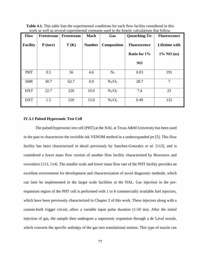
77

Table 4.1. This table lists the experimental conditions for each flow facility considered in this

work as well as several experimental constants used in the kinetic calculations that follow.

Flow

Facility

Freestream

P (torr)

Freestream

T (K)

Mach

Number

Gas

Composition

Quenching-To-

Fluorescence

Ratio for 1%

NO

Fluorescence

Lifetime with

1% NO (ns)

PHT 0.5 56 4.6 N2 0.03 191

SHR 30.7 62.7 4.9 N2/O2 28.7 7

HXT 22.7 220 10.0 N2/O2 7.4 23

HXT 1.5 220 15.0 N2/O2 0.49 132

IV.3.1 Pulsed Hypersonic Test Cell

The pulsed hypersonic test cell (PHT) at the NAL at Texas A&M University has been used

in the past to characterize the invisible ink VENOM method in a underexpanded jet [5]. This flow

facility has been characterized in detail previously by Sanchez-Gonzalez et al. [112], and is

considered a lower mass flow version of another flow facility characterized by Bowersox and

coworkers [113, 114]. The smaller scale and lower mass flow rate of the PHT facility provides an

excellent environment for development and characterization of novel diagnostic methods, which

can later be implemented in the larger scale facilities at the NAL. Gas injection in the pre-

expansion region of the PHT cell is performed with 1 to 8 commercially available fuel injectors,

which have been previously characterized in Chapter 2 of this work. These injectors along with a

custom-built trigger circuit, allow a variable input pulse duration (1-50 ms). After the initial

injection of gas, the sample then undergoes a supersonic expansion through a de Laval nozzle,

which converts the specific enthalpy of the gas into translational motion. This type of nozzle can

78

be useful for both low temperature kinetic measurements, since the gas samples are cooled to a

range of temperatures dependent on the Mach number of the nozzle (32 – 200 K), as well as

hypersonic flow measurements and characterization of hypersonic phenomenon previously

mentioned in Chapter 1. This facility can also operate with a range of gases, such as pure nitrogen,

air, and helium. This allows the measurement of a wide range of mode-specific kinetic behavior.

The conditions produced by a Mach 4.6 nozzle in this facility were considered. This included a

stable flow pressure of 0.5 torr and a freestream flow temperature of 56 K. This calculation also

assumes a “write” laser power of 12 mJ/pulse at 226 nm. Three concentrations of NO were

considered, 2%, 5%, and 10%, to analyze the effects of varying the seed concentration. For the

invisible ink method, there is an initial rapid (< 2 μs) temperature rise due to collisional quenching

and subsequent rotational/translational thermalization. From the equipartition prediction via the

prior probability model, approximately 7/11 of the excitation photon energy goes into

rotational/translational energy for a quenching collision in this short timescale. This short-scale

temperature rise is predicted from the total number density of NO present, the laser excitation

energy, the absorption cross section of NO at 226 nm, and the ratio of quenching to fluorescence

for a particular set of flow conditions. This rapid transfer of electronic excitation to

rotational/translational excitation is then followed by rotational/translational thermalization.

Previous measurements have shown translational thermalization occurs after approximately four

collisions, for argon [115]. This translational thermalization was found to strongly depend on the

molecular mass of the collision partners. Rotational thermalization has been previously reported

to occur on the order of 4.2 collisions in a free jet expansion, with a listed range of 3.3 – 7.3

collisions in several different types of flows [116]. For the purposes of this work, it was considered

that 7 collisions results in full rethermalization of rotational/translational energy, and a hard-sphere

79

collision rate was utilized to convert this model from collision-space to time-space. This rapid

temperature rise is then subsequently followed by a slower (> 10 ms) temperature rise due to

vibrational rethermalization. This secondary rise is particularly slow in the PHT facility, due to the

relatively low density of gas in the flow. A plot of this vibrational rethermalization can be seen in

Figure 4.5 below. In this figure, various time delayed vibrational distributions are displayed

immediately following the “write” laser excitation from the invisible ink method. The black data

represents the final thermodynamic equilibrium, where the initial vibrational excitation has fully

rethermalized.

80

Figure 4.5. This plot displays the vibrational relaxation of v = 0-22 in the PHT facility for 2%

NO seeding at the conditions previously described. The times given in the legend refer to the

time delays after the initial “write” laser of the invisible ink method. The black data represents

the final vibrational distribution expected at thermodynamic equilibrium.

The secondary temperature rise is calculated by monitoring the change in vibrational

energy overtime with the previously described kinetics model. The total energy in all vibrational

modes (for each molecule) is calculated for every time step and a heat capacity calculation is

performed to determine the increase in temperature for that time step. The scales of these two

81

temperature rises for each concentration of NO tested can be seen below in Table 4.2. It should be

noted that Trapid refers to the short timescale temperature rise and Tfinal refers to the temperature

after total vibrational rethermalization. The ratio of quenching to fluorescence is also listed to

better display the relationship of quenching behavior to both the initial and final temperature rises.

Table 4.2. This table displays the calculated short time (Trapid) and long time (Tfinal) temperature

rises due to the invisible ink method for three different seed concentrations of NO. QF Ratio

refers to the ratio of quenching to fluorescence for a given set of conditions.

% NO QF Ratio Tinitial (K) Trapid (K) Tfinal (K)

2 0.056 56 56.1 57.5

5 0.140 56 56.8 58.9

10 0.280 56 58.8 62.4

On the timescale of a VENOM measurement, Trapid is the main temperature perturbation of

concern. While the long time temperature rise does occur, the timescale of Tfinal is longer than the

residence time in the PHT facility. However, it should be noted for slow flows or rapid sampling

of a flow, this long timescale of vibrational relaxation can cause major issues for a VENOM

measurement, and thus, should be calculated to better predict impacts of the technique to a flow

field. For example, if there is a large build-up of vibrational excitation in the testing region of the

flow, and the testing region is not subsequently fully refreshed in between measurements, the

efficacy of the VENOM method will drop considerably, since the “write” grid of vibrational

excitation will be mixed with the large amount of vibrational excitation already present.

For the PHT facility, the rapid temperature rise is relatively low, providing 0.2% - 4.7%

flow perturbation for the concentrations of NO considered, comparable to the normal uncertainty

of a VENOM measurement of 5% - 10% in temperature. This temperature perturbation is largely

dependent on the concentration of NO, which impacts quenching behavior in an otherwise purely

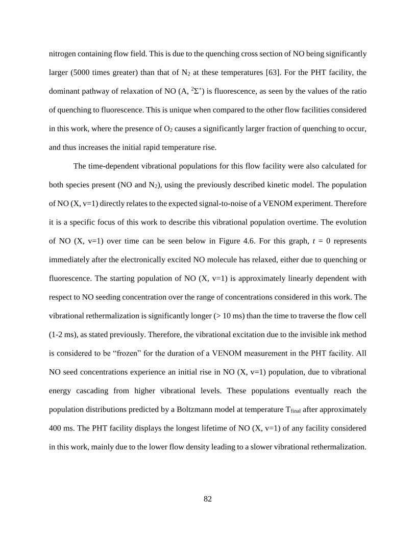
82

nitrogen containing flow field. This is due to the quenching cross section of NO being significantly

larger (5000 times greater) than that of N2 at these temperatures [63]. For the PHT facility, the

dominant pathway of relaxation of NO (A, 2Σ+) is fluorescence, as seen by the values of the ratio

of quenching to fluorescence. This is unique when compared to the other flow facilities considered

in this work, where the presence of O2 causes a significantly larger fraction of quenching to occur,

and thus increases the initial rapid temperature rise.

The time-dependent vibrational populations for this flow facility were also calculated for

both species present (NO and N2), using the previously described kinetic model. The population

of NO (X, v=1) directly relates to the expected signal-to-noise of a VENOM experiment. Therefore

it is a specific focus of this work to describe this vibrational population overtime. The evolution

of NO (X, v=1) over time can be seen below in Figure 4.6. For this graph, t = 0 represents

immediately after the electronically excited NO molecule has relaxed, either due to quenching or

fluorescence. The starting population of NO (X, v=1) is approximately linearly dependent with

respect to NO seeding concentration over the range of concentrations considered in this work. The

vibrational rethermalization is significantly longer (> 10 ms) than the time to traverse the flow cell

(1-2 ms), as stated previously. Therefore, the vibrational excitation due to the invisible ink method

is considered to be “frozen” for the duration of a VENOM measurement in the PHT facility. All

NO seed concentrations experience an initial rise in NO (X, v=1) population, due to vibrational

energy cascading from higher vibrational levels. These populations eventually reach the

population distributions predicted by a Boltzmann model at temperature Tfinal after approximately

400 ms. The PHT facility displays the longest lifetime of NO (X, v=1) of any facility considered

in this work, mainly due to the lower flow density leading to a slower vibrational rethermalization.

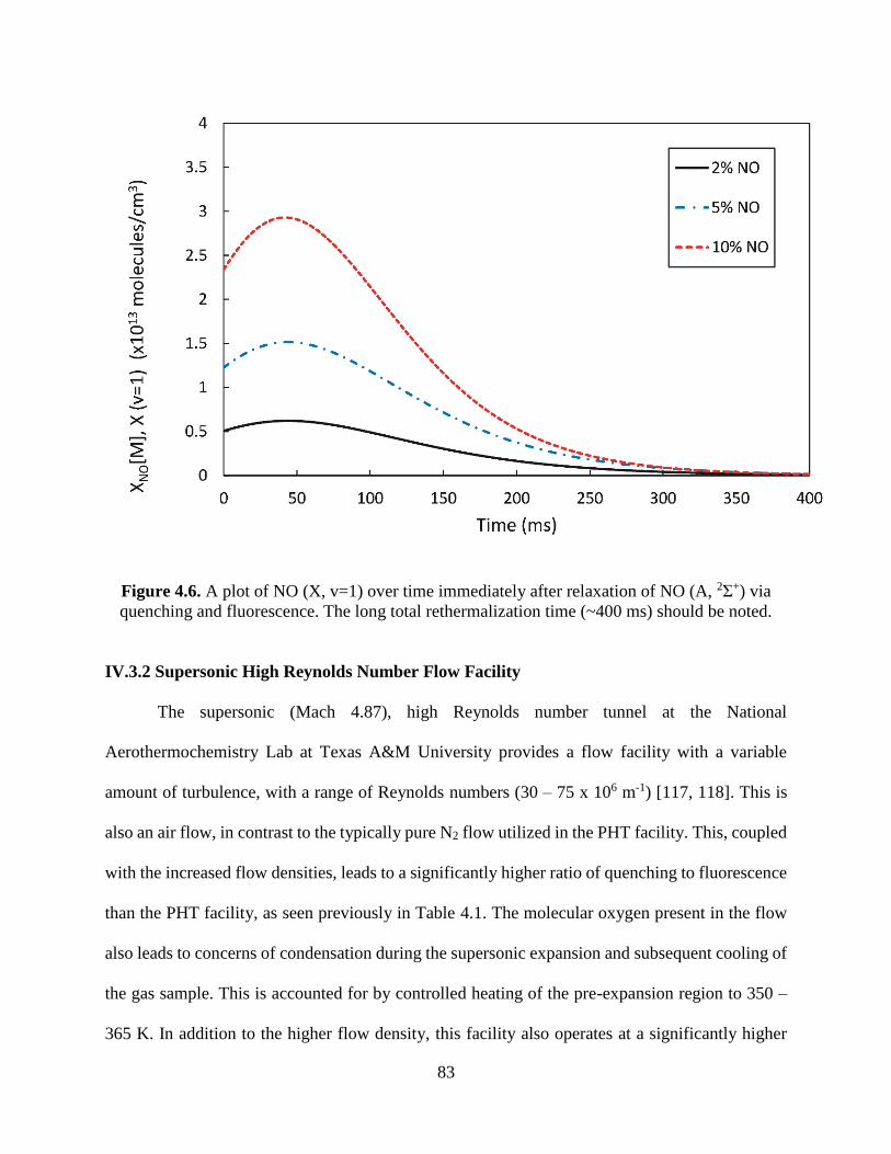
83

Figure 4.6. A plot of NO (X, v=1) over time immediately after relaxation of NO (A, 2Σ+) via

quenching and fluorescence. The long total rethermalization time (~400 ms) should be noted.

IV.3.2 Supersonic High Reynolds Number Flow Facility

The supersonic (Mach 4.87), high Reynolds number tunnel at the National

Aerothermochemistry Lab at Texas A&M University provides a flow facility with a variable

amount of turbulence, with a range of Reynolds numbers (30 – 75 x 106 m-1) [117, 118]. This is

also an air flow, in contrast to the typically pure N2 flow utilized in the PHT facility. This, coupled

with the increased flow densities, leads to a significantly higher ratio of quenching to fluorescence

than the PHT facility, as seen previously in Table 4.1. The molecular oxygen present in the flow

also leads to concerns of condensation during the supersonic expansion and subsequent cooling of

the gas sample. This is accounted for by controlled heating of the pre-expansion region to 350 –

365 K. In addition to the higher flow density, this facility also operates at a significantly higher

84

mass flow rate than the PHT facility at similar Mach numbers. Overall, the SHR facility provides

a well characterized supersonic turbulent boundary layer. This provides an ideal environment to

test the efficacy of the invisible ink technique for simultaneous single-shot velocimetry and

thermometry, and several unique challenges when compared to the previous PHT facility. One

major concern is the previously mentioned heightened level of quenching, due to both higher gas

densities as well as the presence of molecular oxygen. This both results in significantly more

thermal perturbation to the SHR facility due to the invisible ink method, as well as a decrease in

the detectable fluorescence signal, which is required in the “read” measurements. This becomes

especially worrisome as the total decay rate of NO (A, 2Σ+) approaches the pulse width of the

“read” laser system (~10 ns). These predicted decays can be seen visually in Figure 4.7 below,

with a comparison to the intrinsic rate of fluorescence of NO (A, 2Σ+). The fluorescence signal

intensities are scaled to 1 for the sake of comparison. There is comparatively little difference from

the intrinsic rate of fluorescence for the PHT facility. However, the SHR facility undergoes such

a significant amount of quenching that the predicted fluorescence decay becomes comparable to

the timescale of laser scatter, which is directly related to the laser pulse width of 10 ns.

85

Figure 4.7. Predicted fluorescence decay rates for the PHT, SHR and HXT flow facilities, along

with the intrinsic rate of fluorescence for NO (A, 2Σ+). All decay rates were calculated for the

conditions listed in Table 4.1, utilizing 5% NO seeding.

Compared to the nitrogen flow utilized in the PHT facility, the SHR facility is an air-

containing flow, which creates two additional pathways of relaxation for vibrationally excited NO

generated by the invisible ink method: vibrational to translational/rotational NO-O2 energy transfer

and near-resonant vibrational-vibrational energy transfer from NO to O2. The rates of these two

processes were defined previously in this chapter. Because of these processes, as well as the

significantly higher flow densities in the SHR facility when compared to the PHT facility, the

timescales and magnitude of temperature perturbations differ significantly in the SHR facility.

This is predominantly due to electronic quenching, leading to larger short timescale (< 2 μs)

temperature perturbations. The subsequent vibrational rethermalization also occurs on a much

86

faster timescale for the SHR facility when compared to the PHT facility. These temperature

perturbation effects for SHR can be seen below in Figure 4.8. For this plot, t = 0 refers to the time

immediately following the “write” excitation laser pulse in the invisible ink method. The initial

rapid rise (~10-7 s) represents the short timescale temperature rise due to electronic quenching and

subsequent rotational/translational thermalization of NO (A, 2Σ+). The stable temperature

following this rapid rise, prior to vibrational rethermalization, is represented by Trapid in Table 4.3

below.

Figure 4.8. A plot of the time-dependent temperature rise in the SHR facility using a NO seed

concentration of 5%. The short-term and long-term temperature rises are separated by vertical

dotted lines and clearly display two distinct time regimes.

87

Table 4.3. This table displays the short-term and long-term temperature rises calculated for the

SHR flow facility for a range of NO seed concentrations. Also of note is the ratio of quenching

to fluorescence for these flow conditions, represented by QF Ratio. Trapid is due to electronic

quenching and subsequent rotational/translational rethermalization while Tfinal includes the final

long-time (> 1 ms) flow temperature after vibrational rethermalization.

% NO QF Ratio Tinitial (K) Trapid (K) Tfinal (K)

2 30.3 62.7 65.1 67.6

5 35.0 62.7 68.7 72.9

10 42.9 62.7 74.7 81.8

The values presented in Table 4.3 show a clear increase in the temperature perturbation due to the

invisible ink method in the SHR facility compared to the PHT flow facility for both the rapid short-

term temperature rise, which occurs on the timescale of a VENOM measurement (< 2 μs) as well

as the longer timescale temperature rise due to vibrational thermalization (>1 ms). This long-term

temperature rise also occurs significantly faster in the SHR facility than the PHT facility. This is

almost entirely due to the increased flow density, which is nearly two orders of magnitude higher

in the SHR facility than the PHT facility. Predicted short timescale temperature rises reach 4%

when using 2% NO seeding and 19% when using 10% NO seeding. This latter perturbation is

larger than the normal inherent error in temperature determination for the VENOM method (5-

10%), and would be considered the main source of error for experiments performed with this high

level of NO seeding. Because of this, it may be beneficial to experimentally “tune” the

concentration of NO used, where the temperature perturbation caused by higher amounts of NO

seeding is weighed against the improvements in signal to noise for a given experiment. The larger

long timescale temperature rise in SHR when compared to PHT should also be noted. This is also

due to the increased level of quenching in the SHR facility. As seen previously in the prior

probability model, the predicted vibrational population in NO due to quenching includes higher

88

vibrational states containing significant amounts of population (see Figure 4.4). This is the cause

of the larger long timescale temperature rise as well as the larger short timescale temperature

perturbation. This can also be thought of conceptually by considering fluorescence. A large portion

of the initial excitation energy is lost in the emitted photon for the fluorescence pathway, while the

total excitation energy is conserved in the molecular collision resulting in quenching.

For a flow facility such as SHR, which is predicted to have large thermal perturbations at

higher NO seeding concentrations, it is beneficial to compare the temperature rises due to the

invisible ink method to those generated by the NO2 photodissociation method. To do this, two

scenarios in the SHR tunnel are considered for each method, with each scenario producing the

same number density of NO (X, v=1) present for a given set of flow conditions. For the invisible

ink method, seeding 5% NO into the facility is predicted to result in 3.6 x 1016 molecules/cm3 of

NO (X, v=1) subsequently produced by the “write” laser grid. To replicate this number density of

NO (X, v=1) utilizing the NO2 photodissociation method, approximately 1.8% NO2 would be

required, assuming 100% excitation of the NO2 present with a 355 nm laser pulse [119]. This

would result in a short timescale temperature rise of 14.7 K, which far exceeds the 6.0 K

temperature rise predicted when using the invisible ink method. The NO2 photodissociation

method also produces O (3P), which greatly enhances the rate of vibrational relaxation of NO (X,

v=1) [120]. This can result in the vibrational rethermalization of NO to result in a temperature

perturbation on the timescale of a VENOM measurement, adding yet another source of increased

temperature for the NO2 photodissociation method when compared to the invisible ink VENOM

variant.

89

IV.3.3 High Enthalpy Expansion Tunnel

The high enthalpy expansion tunnel (HXT) has recently been constructed at the National

Aerothermochemistry Lab (NAL) at Texas A&M University. While other flow facilities at the

NAL rely on the supersonic expansion of a near room temperature gas, the HXT facility operates

by creating a high enthalpy shock in the test gas sample. This results in significantly higher

freestream temperatures post-expansion. This facility is predicted to operate with a freestream flow

temperature of 220 K after expansion. To create this high enthalpy hypersonic flow, an inert driver

gas (~2000 psi) is initially prepared and separated from a test gas region (~350 psi) by a double

diaphragm, which contains some pressure between the two diaphragms to prevent rupture. This

test gas region can be filled with any gas of interest, including air, N2 and noble gases. The region

between the double diaphragm is then evacuated, causing the two diaphragms to burst and

accelerate the driver gas through the test gas region, creating a shock wave. This shock wave then

bursts a single diaphragm on the other side of the test gas section. This gas sample is then

accelerated in a constant area expansion region. This expansion region can then terminate at a

testing section or a nozzle can be implemented before the test section to further accelerate the gas

sample. Fundamental testing of this new facility is still being performed at the time of writing this

work. A diagram of the HXT flow facility can be seen below in Figure 4.9. The characterization

of a high enthalpy turbulent boundary layer in the HXT facility by the invisible ink VENOM

technique is currently planned. Therefore, the modelling of expected temperature perturbations

and signal to noise for this method will provide valuable information about the efficacy of this

technique in a novel flow facility.

90

Figure 4.9. An experimental diagram of the HXT facility. The acceleration region has been

truncated for posting here. The conditions and regions of the facility are clearly labelled.

Calculations presented in this work have been performed for a final freestream flow

pressure of 22.7 torr, a freestream flow temperature of 220 K, operating conditions at Mach 10,

and an expected Reynolds number of 1 x 107 m-1. The high temperature shock produced by this

facility is expected to result in the nascent formation of NO. This formation of NO can be predicted

by a thermodynamic equilibrium calculation [121]. This calculation included the dissociation of

N2, O2, and NO as well as the formation of all three molecular species as well as N and O atoms.

The predicted percentages of formation of NO in HXT can be seen below in Figure 4.10. With the

shock wave produced in HXT predicted to reach 2000 K, a concentration of ~0.8% NO is expected.

91

Figure 4.10. This plot displays the predicted concentration of NO in the HXT flow facility for a

range of flow temperatures. This was determined through a thermodynamic equilibrium

calculation [121].

It should be noted that this calculation represents the final thermodynamic equilibrium at

some arbitrarily large time delay. For this reason, 0.8% NO represents an upper bound on the

expected formation of nascent NO in the HXT facility. In future studies, it would be beneficial to

examine the kinetic rates of the various processes considered in this thermodynamic calculation,

to determine the speed at which nascent NO is formed, and to further assess the prediction of 0.8%

NO. This could also include the seeding of NO into the test section, if the formation of NO is

limited in a kinetic model.

Prior to expansion in HXT, the gas is assumed to be in thermodynamic equilibrium at 2000

K. For this reason, the vibrational, rotational, and translational distributions of the present gases

are described as a Boltzmann distribution at this temperature. During expansion, this gas sample

92

is predicted to cool to ~ 220 K. As seen previously in the PHT and SHR flow facilities, vibrational

rethermalization can take significantly longer than rotational/translational thermalization.

Therefore, it is unclear if the final gas sample will have a vibrational temperature of 2000 K, 220

K or somewhere in between. Because of this uncertainty, this work includes modelling of the HXT

facility with two limiting cases; one case where the vibrational temperatures of NO, O2 and N2

present are started at 2000 K at the beginning of the vibrational kinetic calculation, to match the

pre-expansion temperature, and a second case where the vibrational temperature has rethermalized

to 220 K to match the rotational/translational energy modes of the flow after reaching the test cell.

For both vibrational temperatures tested, the same concentration of NO has been assumed, and

matches the previously described thermodynamic equilibrium prediction of 0.8 % NO.

A one-dimensional kinetic model has been performed to make a more accurate prediction

of the vibrational temperatures of the three molecular species present. The calculation predicted a

vibrational temperature of 495 K for NO, 1900 K for O2 and nearly 2000 K for N2. This calculation

utilized the acceleration time as well as V-T and V-V energy transfer for all three species. The

relatively low vibrational temperature of NO is a result of the significantly faster V-T rate of NO

with the three diatomic species present. Likewise, V-T energy transfer for O2 is significantly faster

than V-T in N2, with the final N2 vibrational temperature expected to have negligible relaxation at

the time of probing the test region of HXT. It should also be noted that V-V relaxation of O2 and

N2 and subsequent V-T relaxation of NO does not provide a sufficiently faster pathway than just

V-T relaxation in N2 and O2 and thus, the vibrational rethermalization of these two diatomics

cannot be redistributed through the faster relaxing NO V-T pathway. Since three distinct

vibrational temperatures are expected in this flow, along with a single temperature describing

rotational/translation energy, we consider the computational simulations where vibrational

93

temperatures are 2000 K and 220 K to be a fair representation of the freestream flow conditions at

the test section.

The vibrational excitation created by the “write” laser step in the invisible ink VENOM

technique is found to begin rethermalization on the timescale of the “read” measurement (< 2 μs).

This is due to the larger rate of V-T energy transfer in the HXT facility when compared to the PHT

and SHR facilities. This larger energy transfer rate is a direct result of the higher operating

temperatures of HXT. For the HXT and SHR facilities running at the same gas densities, the

temperature differences between the two flow fields (220 K and 62.7 K respectively) will result in

a predicted V-T rate 23 times higher in HXT than SHR. Due to this partial vibrational

rethermalization, probing the flow at different downstream positions in the test section of HXT

could result in vastly different levels of vibrational excitation, resulting both from the invisible ink

VENOM method as well as the high temperature (2000 K) shock wave created in HXT and

subsequent NO formation. This is an important concern to consider with the VENOM method,

which relies on vibrational excitation tagging of the flow field and enough NO (X, v=1) generation

to resolve the differences in the tagging region NO (X, v=1) population and the levels of

background NO (X, v=1) already present.

A direct comparison of the time-dependent evolution of NO (X, v=1) for the two

simulations modelling vibrational temperatures of 220 K and 2000 K is shown below in Figure

4.11. The blue dashed line refers to the calculation performed where the rotational/translational

temperature of the flow field is initialized at 220 K, while the vibrational temperatures of NO, O2

and N2 are initialized at 2000 K. The red line refers to the calculation where all energy modes

present in the flow, including vibrations, are initialized at 220 K prior to the “write” laser of the

invisible ink technique. Time zero on this plot is a result of the prior probability calculation,

94

Franck-Condon populations and Boltzmann distributions of vibrations previously described for

these temperatures and laser fluences. The dotted vertical black line refers to the timescale of a

VENOM measurement (< 2 μs). Both calculations were performed for flows containing 1% NO

present, to mimic the results predicted from nascent NO formation at the pre-expansion

temperature of 2000 K (~0.8%). For the calculation with vibrational energy initialized at 220 K,

the population of NO (X, v=1) caused by thermal energy is approximately 0.0003% of the total

NO number density present, and the “write” laser step of the invisible ink method is can be

considered as responsible for nearly all NO (X, v=1) present at t = 0. This red curve is similar to

the previous calculations of NO (X, v=1) in SHR and PHT, with an initial increase in NO (X, v=1)

due to vibrational cascading from higher excited levels of vibrations. There is also a modest

temperature rise of approximately 1.3 K as this vibrational relaxation occurs. In general,

temperature perturbations due to the invisible ink method in HXT are relatively low when

compared to those for PHT and SHR. For the sample initiated with a 2000 K vibrational

temperature, the time-dependent population of NO (X, v=1) is predicted to monotonically

decrease, which is a result of the higher temperature vibrational modes rethermalizing with the

rotational/translational temperature of the flow.

95

Figure 4.11. This plot shows the time dependence of the two different simulations of NO (X,

v=1) in the HXT facility. The dotted black vertical line is included for clarifying the timescale of

a VENOM measurement on the logarithmic “time” axis.

For the simulation including vibrational energy initialized at 2000 K, meant to model

inefficient vibrational rethermalization from the high temperature shock wave generated in the

HXT facility, there is a nonnegligible contribution to the population of NO (X, v=1) resulting from

the temperature of the vibrational modes prior to excitation by the invisible ink “write” laser

system. However, the invisible ink VENOM method “write” excitation results in a 273%

enhancement in NO (X, v=1) over this nascent population, which is expected to provide adequate

perturbation to discriminate against non-“written” regions of the flow. The overall vibrational

relaxation for this higher vibrational initial temperature calculation is a result of the increased rate

of V-T resulting from the elevated flow temperature. While the population of NO (X, v=1) remains

stable over the timescale of a VENOM measurement for the sample initialized with total

96

vibrational/rotational/translational thermalization to 220 K post-expansion (<0.1% total change),

this is not the case for the sample with initial vibrational non-equilibrium, which has a change of

approximately 2.6% of the NO (X, v=1) population on this timescale. This type of decrease in NO

(X, v=1) population over these relatively short timescales could result in inaccuracies with respect

to the temperature measurement performed in the VENOM method. For instance, in this

simulation, the population of the first “read” laser sheet would be slightly higher than the second

“read” laser sheet than expected based purely on temperature dependence. However, the impact of

this 2.6% decrease in NO (X, v=1) may not result in a drastic error in the measurement of flow

temperature. As a specific example, if one was using rotational states of j = 1.5 and j =10.5 for the

first and second “read” laser sheets respectively, a measured temperature of 216 K would result

for a flow field with a temperature of 220 K. If the high j and low j laser sheet order is reversed,

this would result in a temperature measurement of 225 K instead of the expected 220 K.

For both simulations presented in the HXT flow facility section, the temperature

perturbation caused by the invisible ink VENOM method is negligible, resulting in short term

temperature rises of approximately 1-2 K. Figure 4.12 below shows the time dependent population

of NO (X, v=1) for the calculation performed with the initial vibrational temperature set to 2000

K. The dotted area under the curve can be thought to represent the overall perturbation due to the

invisible ink “write” step over the background of nascent NO (X, v=1) at this higher temperature.

The lower amount of an overall temperature perturbation can be thought of as both a result of the

lower number densities of total NO expected in this facility as well as the relative decrease in

quenching efficiency at these higher temperatures, specifically when compared to the SHR facility.

For the long timescale heating of the flow field, the majority of heating is due to the

97

rethermalization of the NO, O2, and N2 vibrational temperatures, which give a predicted total

temperature rise of 129 K for this simulation.

Figure 4.12. A plot of the time dependent evolution of NO (X, v=1) following the “write” laser

pulse in the invisible ink VENOM method. The dotted horizontal line refers to the vibrational

population at the final vibrational temperature of the flow of ~349 K. The shaded region

represents the additional population of NO (X, v=1) resulting from the “write” laser excitation.

The impact of self-absorption for should also be noted for the three flow facilities in this

chapter. The “read” laser sheet for a VENOM measurement utilizes the (1-1) transition for the NO

(A, 2Σ+) ← NO (X, 2Π) system. Approximately 35% of the total fluorescence emitted from NO

(A, v=1) is associated with the (1-0) transition and approximately 10% results from the (1-1)

transition. Since the PHT and SHR facilities both generate cold flows, and since NO is essentially

98

entirely in v=1 at these temperatures, only the emission associated with the (1-0) transition should

be considered when determining the self-absorption effects. For the PHT facility operating with

1% NO seeding, this results in approximately 4% of the total fluorescence signal being self-

absorbed. For the SHR facility, gas density present and path length of the fluorescence out of the

cell are both larger than seen in the PHT facility. For these reasons, the emission due to the (1-0)

transition are expected to be fully absorbed, which results in a total decrease in fluorescence signal

of 35% due to self-absorption. For the HXT flow facility, if the vibrational temperature at the test

section is ~220 K, the same decrease in fluorescence signal of 35% is predicted, due to total

absorption of the (1-0) transition. However, if the test gas reaching the test section has a vibrational

temperature of 2000 K, the emission from the (1-1) transition should also be considered for self-

absorption. Accounting for the vibrational populations of v=0 and v=1 at this vibrational

temperature of 2000 K, and the relative amounts of the total emission due to the (1-0) and (1-1)

transitions, the total reduction of fluorescence signal due to self-absorption is found to be ~44%.

IV.4 Conclusion

A detailed statistical analysis of the invisible ink VENOM method has been presented here,

with the applicability examined for three distinct flow facilities at the National

Aerothermochemistry Lab at Texas A&M University. These facilities include a pulsed hypersonic

test facility, a high Reynolds number turbulent boundary layer facility, and a high enthalpy

expansion tunnel. Overall, the invisible ink method is predicted to effectively generate the

vibrationally excited samples of NO needed for the VENOM method in all three flow facilities.

For the PHT facility, the temperature perturbations caused by the invisible ink method are found

to be minimal at reasonable concentrations of seeded NO. For the SHR facility, which has

99

significantly higher collisional quenching than the PHT facility due to both higher flow density as

well as the presence of molecular oxygen, was predicted to have more significant temperature

perturbations on the timescale of a VENOM measurement, due to the initial energy from the

“write” photon in the invisible ink technique being redistributed via collisional quenching and then

undergoing a rapid rotational/translation thermalization, which occurs in less than 10 total

collisions. This higher level of collisional quenching in the SHR facility will also lower the total

fluorescence signal of a VENOM experiment. This requires a sophisticated detection system or

filtering as the total fluorescence lifetime approaches the “read” laser pulse width (~10 ns). For

the HXT facility, variance in the vibrational population of NO on the timescale of a VENOM

measurement was predicted, due to the faster rate of V-T energy transfer at the higher operating

temperatures of this facility. However, this variance has limited impact on the temperature

determination performed in a VENOM measurement.

100

CHAPTER V

CONCLUSION AND FUTURE WORK

V.1 NO Injection in Hypersonic Wind Tunnels

The invisible ink VENOM method previously described in Chapters 1 and 4 requires the

seeding of NO as a tracer species. For the PHT facility, this involves premixing pure NO gas

with N2 prior to expansion. However, for the larger scale flow facilities located at the NAL, a

large compressor system is used for preparing an initial sample of air for hypersonic expansion.

Thus, it becomes financially impractical to seed NO into this pre-expansion system, similar to

the previous method in the PHT flow field. Direct injection of pure NO into the flow during or

after the hypersonic expansion is currently being tested for these two facilities. This involves the

same fuel injector systems described previously in Chapter 2 operating with pure NO and

coupled to ACE or SHR.

For the SHR and ACE facilities, NO injection has been tested utilizing a high pressure

container coupled to the expansion regions of these facilities. An image of this container can be

seen below in Figure 5.1. The fuel injector system is contained within this high pressure

container for two reasons. The first concern of this system is the safety of the new NO injection

line. The pressure ratings of both the SHR and ACE facility are ~ 600 psi, so this high pressure

containment cell prevents the fuel injector system from being a point of failure for any

unforeseen issues of high pressurization. The second reason for this system is the fuel injector

ceases to function if the difference in pressure from outside the injector is greater than 100 psi.

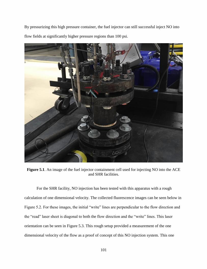
101

By pressurizing this high pressure container, the fuel injector can still successful inject NO into

flow fields at significantly higher pressure regions than 100 psi.

Figure 5.1. An image of the fuel injector containment cell used for injecting NO into the ACE

and SHR facilities.

For the SHR facility, NO injection has been tested with this apparatus with a rough

calculation of one dimensional velocity. The collected fluorescence images can be seen below in

Figure 5.2. For these images, the initial “write” lines are perpendicular to the flow direction and

the “read” laser sheet is diagonal to both the flow direction and the “write” lines. This laser

orientation can be seen in Figure 5.3. This rough setup provided a measurement of the one

dimensional velocity of the flow as a proof of concept of this NO injection system. This one

102

dimensional velocity determination can be seen in Figure 5.4, with the velocity profile matching

the predicted shape of a turbulent boundary layer. For the SHR facility, the NO injection system

was directly sent through an opening at the bottom of the pre-expansion region, with no concern

of spatially uniform seeding. Thus the relative NO concentration may be larger close to the walls

of the flow field, when compared to the freestream NO concentration.

Figure 5.2. Fluorescence images of the “write” and “read” laser fluorescence in the SHR

velocimetry measurement. For these measurements, t0 refers to the time of the initial “write”

laser entering the flow field.

103

Figure 5.3. The experimental layout of the NO injection system tests in the SHR facility.

104

Figure 5.4. The determined one-dimensional velocity in the SHR facility for the testing of the

NO injection system.

This NO injection system is currently being tested in the ACE facility as well. Since this

flow field is much more laminar than the SHR facility, spatial seeding of the NO needs to be

accounted for. Simply injecting a pure sample of NO at the wall may not result in sufficient NO

number densities in all regions of interest for the facility. For this reason, an oblique pipe has been

designed to inject NO on the centerline of the ACE facility. The first and second iteration of this

pipe can be seen below in Figure 5.5. The first iteration involved holes drilled along of the length

of the pipe to inject NO along the vertical axis of the flow field. The second version of this pipe

105

uses a slit, instead of discrete holes, due to early concerns that the NO was choked by the smaller

holes on the previous version of the pipe.

Figure 5.5. The first and second versions of the NO injection pipe used for the ACE facility

106

For the testing in SHR, the injector was used at a duty cycle where it was open 90% of the

time. This gave large amounts of NO in the facility (see Figure 5.2) but also resulted in the rather

inefficient usage of pure NO. For the ACE facility, the objective is to shorten the open time of the

injection system as much as feasible, to conserve the usage of NO in the facility. For this reason,

initial timing studies were performed and the time delay between the fuel injector engaging and

NO being detected in the test region of the facility was found to be approximately 12 ms, with a

stable concentration being achieved after 18 ms. Sample images of the detected fluorescence in

the ACE facility can be seen below in Figure 5.6. For these images, the flow direction is top to

bottom and the laser beam is sent in perpendicular to the flow direction. It is clear from the images

that the equatorial spread of NO is limited for the ACE facility, as predicted due to the lower

operating Reynold’s number of the facility when compared to the SHR facility. However, for these

images taken with a laser line, there are clearly several inhomogeneities that are not reproducible

from image to image.

107

Figure 5.6. Images of NO fluorescence within a single run in the ACE facility.

To further assess the cause of the inhomogeneities across the line of fluorescence signal, a

small laser sheet was formed and the facility was subsequently tested using the same flow

conditions. These images can be seen in Figure 5.7. It is clear from these images that there are

strong vortices present in the flow field, which is the cause of the nonuniform NO seeding across

this region. These vortices are theorized to result from the pipe used for NO injection. While the

pipe was deformed to be oblique and less cylindrical, it likely still has the effect of creating the

vortices seen in Figure 5.7.

108

Figure 5.7. Three images of NO fluorescence from a small laser sheet in the ACE facility. The

flow direction is from the top of the image to the bottom

Overall, the injection of NO into the larger scale supersonic ACE and SHR facilities at

the NAL still requires a full detailed workup of the time-dependent behavior of the injection

system as well as calculations of the dependence of NO number density on the time the injector

is open, the total pressure differential across the injector, and various different flow conditions

which can be produced in the ACE facility.

109

V.2 Low Temperature Collisional Quenching with Polar Quenchers

The temperature dependent collisional quenching of NO (A, 2Σ+) by benzene and

hexafluorobenzene previously reported in Chapter 3 represents only two quenchers believed to

undergo the resonant energy transfer mechanism. While the quenching cross sections of these

two species are predicted, at low temperature, to have a temperature dependent of T-1/3, as

predicted by a capture cross section model, this temperature dependence is different for a

quencher with a nonzero dipole moment. For quenchers with a nonzero dipole moment, the

temperature dependence from this model is predicted to be T-2/3, due to dipole-dipole and

dispersion forces between NO and the quencher. For this reason, in future quenching studies it

would be beneficial to test quenchers of NO (A, 2Σ+) believed to undergo the resonant energy

transfer model that also contain a nonzero dipole moment, to see if there is this predicted

temperature dependence, which varies from that of benzene and hexafluorobenzene. Table 5.1

below lists a series of molecules expected to quench NO (A, 2Σ+) via resonant energy transfer,

along with the total dipole moments, expressed in Debyes. Regardless of the magnitude of the

permanent dipole moment of these molecules, the dipole moment is still predicted to alter the

temperature dependence of the quenching cross section and future studies would allow the

analysis of the capture cross section model with respect to modelling resonant electronic energy

transfer.

110

Table 5.1. This table lists quenchers of NO (A, 2Σ+) which are predicted to act via RET, along

with their respective dipole moments.

Molecular Quencher Dipole Moment (D)

CH3I 1.620

Toluene 0.332

NH3 1.470

CF3I 1.048

SO2 1.630

V.3 Future Updates to Kinetics Simulations for HXT and SHR

The kinetic simulation program described in Chapter 4 operates by explicitly solving all

differential equations for each time-step. Although this does give correct results for every time-

step, this method has several shortcomings. For systems where there are several different

timescales in the kinetic processes of interest (i.e. “stiff” systems), this method of solving the

coupled differential equations involved can lead to long runtimes to sufficiently simulate all

species of interest to their final equilibrium conditions. Simply increasing the time-step for these

simulations can result in failures for the program to operate, since the short timescale processes

will now give non-real concentrations (i.e. negative values if the time step is sufficiently large).

For example, in the case of the HXT facility, the vibrational excitation in NO is predicted to

vibrationally thermalize several orders of magnitude faster than that of O2, which is predicted to

vibrationally thermalize several orders of magnitude faster than N2. For simulating these types of

systems, it is computationally inefficient to perform this explicit Euler scheme, merely to confirm

111

the final vibrational distributions of N2 converge to the predicted thermodynamic equilibrium

values.

There are several numerical methods for solving these types of “stiff” partial differential

equation systems, which when implemented, would result in significantly shorter computation

time and resources. In the future, it would be beneficial to implement either one or a combination

of these approximation methods for complex systems with drastically different timescales present.

One specific technique will be briefly discussed in this work, although it should be noted there are

numerous approximation methods for these types of systems; the Runge-Kutta (RK) method.

For the current version of the kinetics program described in Chapter 4, the system of

differential equations relating to the changes in vibrational populations are solved by the Euler

method. This method operates via the equation below

𝑃𝑛+1 = 𝑃𝑛 + 𝛥𝑡 ∗ 𝑓(𝑃𝑛, 𝑀𝑛)

where Pn is the number density of a given vibrational state of interest at step n, Δt is the selected

time-step of the system, M is the number density of the collision partner and f is the total set of

differential equations for the vibrational state of interest. This includes VV and VT rates for all

species present. While this method gives accurate overall solutions for a sufficiently small time-

step, as stated above it has issues of instability when evaluating changes in vibrational populations

that occur on drastically different timescales within a single simulation. The RK method operates

by calculating a change in population at the middle of the interval Δt. This method then uses the

computed values of P and M at this midpoint to compute the change across the entire time-step.

For one mid-point step taken, this is defined as the second-order RK method. The equations for

the second order RK method are shown below for this system.

𝑘1 = 𝛥𝑡 ∗ 𝑓(𝑃𝑛, 𝑀𝑛)

112

𝑘2 = 𝛥𝑡 ∗ 𝑓(𝑃𝑛 +1

2𝑘1, 𝑀𝑛 +

1

2𝛥𝑡)

𝑃𝑛+1 = 𝑃𝑛 + 𝑘2

where k1 and k2 are the half-step solution terms. This can be further extended to the commonly

used fourth-order version of the RK method, which further reduces the error of calculation when

compared to the Euler method for the same time-step size. The equations for the fourth order form

of the RK method are shown below, and match the same formulism as the second order version.

𝑘1 = 𝛥𝑡 ∗ 𝑓(𝑃𝑛, 𝑀𝑛)

𝑘2 = 𝛥𝑡 ∗ 𝑓(𝑃𝑛 +1

2𝑘1, 𝑀𝑛 +

1

2𝛥𝑡)

𝑘3 = 𝛥𝑡 ∗ 𝑓(𝑃𝑛 +1

2𝑘2, 𝑀𝑛 +

1

2𝛥𝑡)

𝑘4 = 𝛥𝑡 ∗ 𝑓(𝑃𝑛 + 𝑘3, 𝑀𝑛 + 𝛥𝑡)

𝑃𝑛+1 = 𝑃𝑛 +𝑘16+𝑘23+𝑘33+𝑘46

This fourth-order version can utilize double the time-step of the second-order version with the

same final accuracy in the newly determined number density of a vibrational state. The RK method

is shown here as one of the simplest methods of solving “stiff” differential equations, as is required

in the model described in Chapter 4. However it should also be noted that methods such as semi-

implicit extrapolation and Gear’s backwards differential method can also be utilized for this

purpose.

A key feature in switching to the RK method over the Euler method is in the adaptive

control of the simulation time-step size. As certain vibrational populations reach equilibrium, the

time-step should adaptively increase to faster simulate the slower vibrational relaxations present.

This prevents convergence errors seen when using large time-steps in the Euler method from the

113

beginning of a simulation. For adapting the time-step of a simulation, the most important factor is

monitoring the amount of error due to the new time-step compared to the previous time-step value.

The simplest form of this adaptive time-step control is known as step doubling. In this method,

each time-step is taken twice; one full time-step and one half time-step. To show how this method

operates, we can define the “true” number density of a vibrational state after some time-step 2Δt

as P(t0+2Δt). The two approximate solutions are defined as P1 (one total time-step of size 2Δt) and

P2 (two time-steps of size Δt). This “true” solution is related to these numerical approximations by

the equations

𝑃(𝑡0 + 2𝛥𝑡) = 𝑃1 + (2𝛥𝑡)5𝐸

𝑃(𝑡0 + 2𝛥𝑡) = 𝑃2 + 2(𝛥𝑡)5𝐸

where E is some constant error, with magnitude P5(t)/5!. The difference in the two approximations

is related to the error of the calculation by the formula

∆ ≡ 𝑃2 − 𝑃1

This relative error can be kept constant by periodically adjusting the value of Δt for the simulation.

For a fourth-order RK method, Δ scales with (Δt)5. Considering a given error Δ0 for an initial time-

step of Δt0, and the new error, Δ1, associated with changing the time-step to Δt1, the following

equation can be used to correct for a new time-step giving unacceptable values of error.

∆𝑡0 = ∆𝑡1 ∗ |∆0∆1|0.2

This equation can then be used to iterate the time-step of a simulation to determine the permissible

change allowed. This would not have to occur for every single simulation step, but could be

periodically checked throughout the simulation (for example, every 1000 total steps). In the future,

it would be beneficial to modify the kinetics program in Chapter 4 with some approximation

114

method to fix issues due to the “stiffness” of these systems of differential equations. The RK

method presented in this work is merely meant to provide an example of one such solution.

115

REFERENCES

[1] T. Fuller, A. Hsu, R. Bowersox, S. North, The Effect of Vibrational Non-Equilibrium on the

Decay of Grid Generated Turbulence, 47th AIAA Aerospace Sciences Meeting including The

New Horizons Forum and Aerospace Exposition, 2009, pp. 593.

[2] N.A. West, J.D. Winner, R.D.W. Bowersox, S.W. North, Resolving the energy and temperature

dependence of C6H6∗ collisional relaxation via time-dependent bath temperature measurements,

Journal of Chemical Physics 145 (2016) 014308.

[3] R. Sánchez-González, R. Srinivasan, R.D.W. Bowersox, S.W. North, Simultaneous velocity

and temperature measurements in gaseous flow fields using the VENOM technique, Opt. Lett. 36

(2011) 196-198.

[4] R. Sánchez-González, R.D.W. Bowersox, S.W. North, Simultaneous velocity and temperature

measurements in gaseous flowfields using the vibrationally excited nitric oxide monitoring

technique: a comprehensive study, Appl. Opt. 51 (2012) 1216-1228.

[5] R. Sánchez-González, R.D.W. Bowersox, S.W. North, Vibrationally excited NO tagging by

NO(A) fluorescence and quenching for simultaneous velocimetry and thermometry in gaseous

flows, Opt. Lett. 39 (2014) 2771-2774.

[6] J.D. Anderson Jr, Hypersonic and high-temperature gas dynamics, American Institute of

Aeronautics and Astronautics2006.

[7] A. Fiala, R. Hillier, Aerothermodynamics of turbulent spots and wedges at hypersonic speeds,

Fifth European Symposium on Aerothermodynamics for Space Vehicles, 2005, pp. 615.

[8] J. Redford, N. Sandham, G. Roberts, Numerical simulations of turbulent spots in supersonic

boundary layers: effects of Mach number and wall temperature, Progress in Aerospace Sciences

52 (2012) 67-79.

116

[9] T. Cebeci, Analysis of turbulent boundary layers, Elsevier2012.

[10] X. Zhong, X. Wang, Direct numerical simulation on the receptivity, instability, and transition

of hypersonic boundary layers, Annual Review of Fluid Mechanics 44 (2012) 527-561.

[11] J.J. Bertin, R.M. Cummings, Critical hypersonic aerothermodynamic phenomena, Annu. Rev.

Fluid Mech. 38 (2006) 129-157.

[12] P.A. Gnoffo, R.N. Gupta, J.L. Shinn, Conservation equations and physical models for

hypersonic air flows in thermal and chemical nonequilibrium, (1989).

[13] R.N. Gupta, J.M. Yos, R.A. Thompson, K.-P. Lee, A review of reaction rates and

thermodynamic and transport properties for an 11-species air model for chemical and thermal

nonequilibrium calculations to 30000 K, (1990).

[14] R. Stalker, Hypervelocity aerodynamics with chemical nonequilibrium, J Annual Review of

Fluid Mechanics 21 (1989) 37-60.

[15] I. Nompelis, T.W. Drayna, G.V. Candler, -A Parallel Unstructured Implicit Solver for

Hypersonic Reacting Flow Simulation, Parallel Computational Fluid Dynamics 2005,

Elsevier2006, pp. 389-395.

[16] M.J. Wright, G.V. Candler, D. Bose, Data-parallel line relaxation method for the Navier-

Stokes equations, AIAA Journal 36 (1998) 1603-1609.

[17] D. Hash, J. Olejniczak, M. Wright, D. Prabhu, M. Pulsonetti, B. Hollis, P. Gnoffo, M.

Barnhardt, I. Nompelis, G. Candler, FIRE II calculations for hypersonic nonequilibrium

aerothermodynamics code verification: DPLR, LAURA, and US3D, 45th AIAA Aerospace

Sciences Meeting and Exhibit, 2007, pp. 605.

[18] H. Hornung, P. Adam, P. Germain, K. Fujii, A. Rasheed, On transition and transition control

in hypervelocity flow, Proceedings of the Ninth Asian Congress of Fluid Mechanics, 2002.

117

[19] E. Reshotko, Transition issues for atmospheric entry, Journal of Spacecraft Rockets 45 (2008)

161-164.

[20] C. Willert, Stereoscopic digital particle image velocimetry for application in wind tunnel

flows, Measurement Science and Technology 8 (1997) 1465-1479.

[21] N.J. Lawson, J. Wu, Three-dimensional particle image velocimetry: a low-cost 35mm angular

stereoscopic system for liquid flows, Optics and Lasers in Engineering 32 (1999) 1-19.

[22] S. Zhang, Handbook of 3D machine vision: Optical metrology and imaging, CRC press2013.

[23] T. Sakurai, T. Handa, S. Koike, K. Mii, A. Nakano, Study on the particle traceability in

transonic and supersonic flows using molecular tagging velocimetry, J Visualization 18 (2015)

511-520.

[24] S. Krüger, G. Grünefeld, Stereoscopic flow-tagging velocimetry, Applied Physics B 69 (1999)

509-512.

[25] M. Koochesfahani, Molecular Tagging Velocimetry (MTV)-Progress and applications, 30th

Fluid Dynamics Conference, 1999, pp. 3786.

[26] R. Miles, W. Lempert, B. Zhang, Turbulent structure measurements by RELIEF flow tagging,

Fluid Dynamics Research 8 (1991) 9-17.

[27] R.B. Miles, D. Zhou, B. Zhang, W.R. Lempert, Z.-S. She, Fundamental turbulence

measurements by RELIEF flow tagging, AIAA Journal 31 (1993) 447-452.

[28] A. Noullez, G. Wallace, W. Lempert, R.B. Miles, U. Frisch, Transverse velocity increments

in turbulent flow using the RELIEF technique, Journal of Fluid Mechanics 339 (1997) 287-307.

[29] P.M. Danehy, S. O'Byrne, A.F. P. Houwing, J.S. Fox, D.R. Smith, Flow-tagging velocimetry

for hypersonic flows using fluorescence of nitric oxide, AIAA Journal 41 (2003) 263-271.

118

[30] C. Orlemann, C. Schulz, J. Wolfrum, NO-flow tagging by photodissociation of NO2. A new

approach for measuring small-scale flow structures, Chemical Physics Letters 307 (1999) 15-20.

[31] A.G. Hsu, R. Srinivasan, R.D.W. Bowersox, S.W. North, Two-component molecular tagging

velocimetry utilizing NO fluorescence lifetime and NO2 photodissociation techniques in an

underexpanded jet flowfield, Appl. Opt. 48 (2009) 4414-4423.

[32] R. Cattolica, OH rotational temperature from two-line laser-excited fluorescence, Appl. Opt.

20 (1981) 1156-1166.

[33] R.K. Hanson, Planar laser-induced fluorescence imaging, Journal of Quantitative

Spectroscopy and Radiative Transfer 40 (1988) 343-362.

[34] C.M. Loe, J.D. Winner, R. Sánchez-González, Thermometry in gas flows using two-line

fluorescence imaging and structured illumination, OSA Continuum 1 (2018) 1185-1194.

[35] M. Luong, R. Zhang, C. Schulz, V. Sick, Toluene laser-induced fluorescence for in-cylinder

temperature imaging in internal combustion engines, Applied Physics B 91 (2008) 669.

[36] R.B. Miles, W.R. Lempert, J.N. Forkey, Laser rayleigh scattering, Measurement Science

Technology 12 (2001) R33.

[37] G.S. Elliott, N. Glumac, C.D. Carter, Molecular filtered Rayleigh scattering applied to

combustion, Measurement Science and Technology 12 (2001) 452-466.

[38] R. Huffman, G. Elliott, An Experimental Investigation of Accurate Particle Tracking in

Supersonic, Rarefied, Axisymmetric Jets, 47th AIAA Aerospace Sciences Meeting including The

New Horizons Forum and Aerospace Exposition, 2009, pp. 1265.

[39] D. Most, A. Leipertz, Simultaneous two-dimensional flow velocity and gas temperature

measurements by use of a combined particle image velocimetry and filtered Rayleigh scattering

technique, Appl. Opt. 40 (2001) 5379-5387.

119

[40] C. Abram, B. Fond, F. Beyrau, Temperature measurement techniques for gas and liquid flows

using thermographic phosphor tracer particles, Progress in Energy Combustion Science 64 (2018)

93-156.

[41] H. Lee, E.K. Kim, S. Kim, Anomalous Propagation Echo Classification of Imbalanced Radar

Data with Support Vector Machine, Advances in Meteorology 2016 (2016) 13.

[42] P. Schreivogel, C. Abram, B. Fond, M. Straußwald, F. Beyrau, M. Pfitzner, Simultaneous

kHz-rate temperature and velocity field measurements in the flow emanating from angled and

trenched film cooling holes, International Journal of Heat and Mass Transfer 103 (2016) 390-400.

[43] R.B. Miles, Optical diagnostics for high-speed flows, 43rd AIAA Fluid Dynamics

Conference, 2013, pp. 2610.

[44] M. Edwards, A. Dogariu, R. Miles, Simultaneous temperature and velocity measurement in

unseeded air flows with FLEET, 51st AIAA Aerospace Sciences Meeting including the New

Horizons Forum and Aerospace Exposition, 2013, pp. 43.

[45] M.R. Edwards, A. Dogariu, R.B. Miles, Simultaneous temperature and velocity measurements

in air with femtosecond laser tagging, AIAA Journal 53 (2015) 2280-2288.

[46] N.J. DeLuca, R.B. Miles, N. Jiang, W.D. Kulatilaka, A.K. Patnaik, J.R. Gord, FLEET

velocimetry for combustion and flow diagnostics, Appl. Opt. 56 (2017) 8632-8638.

[47] Y. Zhang, M.N. Shneider, R.B. Miles, Femtosecond Laser Excitation in Argon–Nitrogen

Mixtures, AIAA Journal 56 (2018) 1060-1071.

[48] N. Jiang, B.R. Halls, H.U. Stauffer, P.M. Danehy, J.R. Gord, S. Roy, Selective two-photon

absorptive resonance femtosecond-laser electronic-excitation tagging velocimetry, Opt. Lett. 41

(2016) 2225-2228.

120

[49] F. Pan, R. Sánchez-González, M.H. McIlvoy, R.D. Bowersox, S.W. North, Simultaneous

three-dimensional velocimetry and thermometry in gaseous flows using the stereoscopic

vibrationally excited nitric oxide monitoring technique, Opt. Lett. 41 (2016) 1376-1379.

[50] G. Herzberg, Molecular Spectra and Molecular Structure, I. Spectra of Diatomic Molecules,

D. Van Nostrand Company Inc1955.

[51] F.M. Behlen, N. Mikami, S.A. Rice, Dynamics of radiationless processes studied in pulsed

supersonic free jets: Some naphthalene lifetimes, Chemical Physics Letters 60 (1979) 364-367.

[52] D. Zakheim, P. Johnson, Two‐ and three‐photon resonances in the four‐photon ionization

spectrum of nitric oxide at low temperature, The Journal of Chemical Physics 68 (1978) 3644-

3653.

[53] N.A. West, J.D. Winner, R.D.W. Bowersox, S.W. North, Resolving the energy and

temperature dependence of C6H6∗ collisional relaxation via time-dependent bath temperature

measurements, J Chem Phys 145 (2016) 014308.

[54] J.R. Barker, Multiple-Well, multiple-path unimolecular reaction systems. I. MultiWell

computer program suite, Int. J. Chem. Kinet. 33 (2001) 232-245.

[55] J.R. Barker, Energy transfer in master equation simulations: A new approach, Int. J. Chem.

Kinet. 41 (2009) 748-763.

[56] G.P. Smith, J.R. Barker, Energy transfer rates for vibrationally excited gas-phase azulene in

the electronic ground state, Chemical Physics Letters 78 (1981) 253-258.

[57] M.J. Rossi, J.R. Barker, Infrared fluorescence and collisional energy transfer parameters for

vibrationally excited azulene*(So): dependence on internal energy (Evib), Chemical Physics

Letters 85 (1982) 21-26.

121

[58] M.J. Rossi, J.R. Pladziewicz, J.R. Barker, Energy‐dependent energy transfer: Deactivation of

azulene (S0, Evib) by 17 collider gases, J Chem Phys 78 (1983) 6695-6708.

[59] A.K. Paul, S.C. Kohale, S. Pratihar, R. Sun, S.W. North, W.L. Hase, A unified model for

simulating liquid and gas phase, intermolecular energy transfer: N2 + C6F6 collisions, J Chem

Phys 140 (2014) 194103.

[60] A.K. Paul, S.C. Kohale, W.L. Hase, Bath Model for N2 + C6F6 Gas-Phase Collisions. Details

of the Intermolecular Energy Transfer Dynamics, The Journal of Physical Chemistry C 119 (2015)

14683-14691.

[61] A.K. Paul, N.A. West, J.D. Winner, R.D.W. Bowersox, S.W. North, W.L. Hase, Non-

statistical intermolecular energy transfer from vibrationally excited benzene in a mixed nitrogen-

benzene bath, J Chem Phys 149 (2018) 134101.

[62] T.B. Settersten, B.D. Patterson, W.H.H. IV, Radiative lifetimes of NO A Σ2+(v′=0,1,2) and

the electronic transition moment of the A Σ2+−X Π2 system, J Chem Phys 131 (2009) 104309.

[63] R. Sánchez-González, W.D. Eveland, N.A. West, C.L.N. Mai, R.D.W. Bowersox, S.W.

North, Low-temperature collisional quenching of NO A2Σ+(v′ = 0) by NO(X2Π) and O2 between

34 and 109 K, J Chem Phys 141 (2014) 074313.

[64] M. Okruss, R. Müller, A. Hese, High-Resolution UV Laser Spectroscopy of Jet-Cooled

Benzene Molecules: Complete Rotational Analysis of theS1←S0610(l= ±1) Band, Journal of

Molecular Spectroscopy 193 (1999) 293-305.

[65] B.S. Olive, Absorption spectra of benzene, toluene, and sulfur dioxide, Results from

measurements at the Department of Chemistry and Industrial Hygiene, University of North

Alabama, Florence, AL, 2015.

122

[66] H. Keller-Rudek, G.K. Moortgat, R. Sander, R. Sörensen, The MPI-Mainz UV/VIS Spectral

Atlas of Gaseous Molecules of Atmospheric Interest, Earth Syst. Sci. Data 5 (2013) 365-373.

[67] H. Zacharias, J.B. Halpern, K.H. Welge, Two-photon excitation of NO(A2Σ+; ν′ = 0,1,2) and

radiation lifetime and quenching measurements, Chemical Physics Letters 43 (1976) 41-44.

[68] G.F. Nutt, S.C. Haydon, A.I. McIntosh, Measurement of electronic quenching rates in nitric

oxide using two-photon spectroscopy, Chemical Physics Letters 62 (1979) 402-404.

[69] I.S. McDermid, J.B. Laudenslager, Radiative lifetimes and electronic quenching rate

constants for single-photon-excited rotational levels of no (A2Σ+, ν′ = 0), Journal of Quantitative

Spectroscopy and Radiative Transfer 27 (1982) 483-492.

[70] M.C. Drake, J.W. Ratcliffe, High temperature quenching cross sections for nitric oxide laser‐

induced fluorescence measurements, 98 (1993) 3850-3865.

[71] M.C. Drake, J.W. Ratcliffe, High temperature quenching cross sections for nitric oxide laser‐

induced fluorescence measurements, J Chem Phys 98 (1993) 3850-3865.

[72] J.A. Gray, P.H. Paul, J.L. Durant, Electronic quenching rates for NO(A 2Σ+) measured in a

shock tube, Chemical Physics Letters 190 (1992) 266-270.

[73] G.D. Greenblatt, A.R. Ravishankara, Collisional quenching of NO(A, v' =0) by various gases,

Chemical Physics Letters 136 (1987) 501-505.

[74] Y. Haas, G.D. Greenblatt, A charge-transfer model for the quenching of electronically excited

nitric oxide. Electron affinity of the quenchers, The Journal of Physical Chemistry 90 (1986) 513-

517.

[75] P.H. Paul, J.A. Gray, J.L. Durant, J.W. Thoman, Collisional electronic quenching rates for

NO A2Σ+ (ν = 0), Chemical Physics Letters 259 (1996) 508-514.

123

[76] G.A. Raiche, D.R. Crosley, Temperature dependent quenching of the A 2Σ+ and B 2Π states

of NO, J Chem Phys 92 (1990) 5211-5217.

[77] T.B. Settersten, B.D. Patterson, C.D. Carter, Collisional quenching of NO A Σ2+(v′=0)

between 125 and 294 K, J Chem Phys 130 (2009) 204302.

[78] T.B. Settersten, B.D. Patterson, J.A. Gray, Temperature- and species-dependent quenching of

NO AΣ+2(v′=0) probed by two-photon laser-induced fluorescence using a picosecond laser, J

Chem Phys 124 (2006) 234308.

[79] R. Zhang, D.R. Crosley, Temperature dependent quenching of A 2Σ+ NO between 215 and

300 K, J Chem Phys 102 (1995) 7418-7424.

[80] M. Asscher, Y. Haas, The quenching mechanism of electronically excited Rydberg states of

nitric oxide, J Chem Phys 76 (1982) 2115-2126.

[81] M.R. Furlanetto, J.W.T. Jr., J.A. Gray, P.H. Paul, J.L.D. Jr., Near‐resonant electronic energy

transfer in the electronic quenching of NO A 2Σ+ by hydrocarbons and ammonia, J Chem Phys

101 (1994) 10452-10457.

[82] G. Briegleb, Electron Affinity of Organic Molecules, 3 (1964) 617-632.

[83] J.J. McGee, J. Heicklen, Photolysis of Nitric Oxide in the Presence of Olefins, J Chem Phys

41 (1964) 2977-2978.

[84] J.W.T. Jr., J.A. Gray, J.L.D. Jr., P.H. Paul, Collisional electronic quenching of NO A 2Σ+ by

N2 from 300 to 4500 K, J Chem Phys 97 (1992) 8156-8163.

[85] T. Forster, Z. Naturforsch., 4a (1949) 321-327.

[86] T. Förster, Zwischenmolekulare Energiewanderung und Fluoreszenz, 437 (1948) 55-75.

[87] T. Főrster, 10th Spiers Memorial Lecture. Transfer mechanisms of electronic excitation,

Discussions of the Faraday Society 27 (1959) 7-17.

124

[88] T. Forster, Energiewanderung und Fluoreszenz, Naturwissenschaften 33 (1946) 166-175.

[89] J. Franck, R. Livingston, Remarks on Intra- and Inter-Molecular Migration of Excitation

Energy, Reviews of Modern Physics 21 (1949) 505-509.

[90] R. Livingston, Intermolecular Transfer of Electronic Excitation, The Journal of Physical

Chemistry 61 (1957) 860-864.

[91] F. Perrin, Théorie quantique des transferts d’activation entre molécules de même espèce. Cas

des solutions fluorescentes, Ann. Phys. 10 (1932) 283-314.

[92] V.I. Vavilov, M.D. Galanin, Dokl. Akad. Nauk USSR 67 (1949) 811-818.

[93] G.D. Scholes, Long-Range Resonance Energy Transfer in Molecular Systems, Ann. Rev.

Phys. Chem. 54 (2003) 57-87.

[94] G. Herzberg, Molecular Spectra and Molecular Structure: IV. Constants of Diatomic

Molecules, Van Nostrand Reinhold, New York, 1966.

[95] G.H. K. P. Huber, Molecular Spectra and Molecular Structure: IV. Constants of Diatomic

Molecules, Van Nostrand Reinhold, New York, 1966.

[96] CRC Handbook of Chemistry and Physics, 83rd ed., CRC Press LLC2002.

[97] C. Motch, A. Giuliani, J. Delwiche, P. Limão-Vieira, N.J. Mason, S.V. Hoffmann, M.J.

Hubin-Franskin, Electronic structure of hexafluorobenzene by high-resolution vacuum ultraviolet

photo-absorption and He(I) photoelectron spectroscopy, Chemical Physics 328 (2006) 183-189.

[98] C. Bing-Ming, L. Hsiao-Chi, C. Hong-Kai, B. Mohammed, L. Yuan-Pern, M.M. Alexander,

L.C. Lee, L. Mao-Chang, L.Y. Yuk, Absorption Cross Sections of NH3, NH2D, NHD2, and ND3

in the Spectral Range 140-220 nm and Implications for Planetary Isotopic Fractionation, The

Astrophysical Journal 647 (2006) 1535.

125

[99] J. Vattulainen, L. Wallenius, J. Stenberg, R. Hernberg, V. Linna, Experimental Determination

of SO2, C2H2, and O2 UV Absorption Cross Sections at Elevated Temperatures and Pressures,

Appl. Spectrosc. 51 (1997) 1311-1315.

[100] W. Koban, J.D. Koch, R.K. Hanson, C. Schulz, Absorption and fluorescence of toluene

vapor at elevated temperatures, Physical Chemistry Chemical Physics 6 (2004) 2940-2945.

[101] S. Eden, P. Limão-Vieira, S.V. Hoffmann, N.J. Mason, VUV photoabsorption in CF3X

(X=Cl, Br, I) fluoro-alkanes, Chemical Physics 323 (2006) 313-333.

[102] S. Eden, P. Limão-Vieira, S.V. Hoffmann, N.J. Mason, VUV spectroscopy of CH3Cl and

CH3I, Chemical Physics 331 (2007) 232-244.

[103] J. Luque, D. Crosley, LIFBASE: Database and simulation program (v 1.6), SRI International

Report MP (1999) 99-009.

[104] J. Luque, D.R. Crosley, Transition probabilities and electronic transition moments of the

A 2Σ+–X 2Π and D 2Σ+–X 2Π systems of nitric oxide, J Chem Phys 111 (1999) 7405-7415.

[105] J.T. Muckerman, Information Theoretic Prior Functions for Large Molecular Systems, The

Journal of Physical Chemistry 93 (1989) 179-184.

[106] B.C.F. S. Nordholm, D. L. Jolly, Ergodic collision theory of intermolecular energy transfer,

Chemical Physics 25 (1977) 433-449.

[107] R.D.L. E. Zamir, Energy disposal in unimolecular elimination reactions, Chemical Physics

52 (1980) 253-268.

[108] M.S. G. Hancock, Vibrational distribution in NO (X 2Π) formed by self quenching of NO

A 2Σ+ (v=0), Physical Chemistry Chemical Physics 10 (2008) 2014-2019.

[109] E.H. Kerner, NOTE ON THE FORCED AND DAMPED OSCILLATOR IN QUANTUM

MECHANICS, Canadian Journal of Physics 36 (1958) 371-377.

126

[110] G.V. Candler, J.D. Kelley, S.O. Macheret, M.N. Shneider, I.V. Adamovich, Vibrational

excitation, thermal nonuniformities, and unsteady effects on supersonic blunt bodies, AIAA

Journal 40 (2002) 1803-1810.

[111] A.C. de Gavelle de Roany, C. Flament, J. Rich, V. Subramaniam, W.R. Warren Jr, Strong

vibrational nonequilibrium in supersonic nozzle flows, AIAA Journal 31 (1993) 119-128.

[112] R. Sánchez-González, R. Srinivasan, J. Hofferth, D.Y. Kim, A.J. Tindall, R.D. W.

Bowersox, S.W. North, Repetitively pulsed hypersonic flow apparatus for diagnostic

development, AIAA Journal 50 (2012) 691-697.

[113] M. Semper, N. Tichenor, R. Bowersox, R. Srinvasan, S. North, On the Design and

Calibration of an Actively Controlled Expansion Hypersonic Wind Tunnel, 47th AIAA Aerospace

Sciences Meeting including The New Horizons Forum and Aerospace Exposition, 2009, pp. 799.

[114] N. Tichenor, M. Semper, R. Bowersox, R. Srinvasan, S. North, Calibration of an actively

controlled expansion hypersonic wind tunnel, 27th AIAA Aerodynamic Measurement

Technology and Ground Testing Conference, 2010, pp. 4793.

[115] G. Nan, P.L. Houston, Velocity relaxation of S(1D) by rare gases measured by Doppler

spectroscopy, The Journal of Chemical Physics 97 (1992) 7865-7872.

[116] D.R. Miller, R.P. Andres, Rotational Relaxation of Molecular Nitrogen, The Journal of

Chemical Physics 46 (1967) 3418-3423.

[117] C. Tilmann, R. Bowersox, T. Buter, On the design and construction of an academic Mach 5

wind tunnel, 37th Aerospace Sciences Meeting and Exhibit, 1999, pp. 800.

[118] I.T. Neel, A. Leidy, R.D. Bowersox, N.R. Tichenor, Hypersonic Boundary Layer with

Streamline Curvature-Driven Adverse Pressure Gradient, 8th AIAA Flow Control Conference,

2016, pp. 4248.

127

[119] M. Hunter, S.A. Reid, D.C. Robie, H. Reisler, The monoenergetic unimolecular reaction of

expansion‐cooled NO2: NO product state distributions at excess energies 0–3000 cm−1, The

Journal of Chemical Physics 99 (1993) 1093-1108.

[120] J.A. Dodd, R.B. Lockwood, E.S. Hwang, S.M. Miller, S.J. Lipson, Vibrational relaxation of

NO(υ=1) by oxygen atoms, The Journal of Chemical Physics 111 (1999) 3498-3507.

[121] D.A. McQuarrie, J.D. Simon, Physical Chemistry: A Molecular Approach, 1st ed.,

University Science Books, USA, 1997.

characterization of collisional energy transfer in …

Documents