characterization and modeling of anisotropic electrically
TRANSCRIPT

Characterization and Modeling of
Anisotropic Electrically Conductive
Composite Filaments comprising PMMA
and Carbon Fillers
Charakterisierung und Modellierung von
anisotropen elektrisch leitfähigen
Komposit-Filamenten aus PMMA und
Carbon Füllstoffen
Der Technischen Fakultät
der Friedrich-Alexander-Universität Erlangen-Nürnberg
zur
Erlangung des Doktorgrades Doktor-Ingenieur
vorgelegt von
Muchao Qu
aus Heilongjiang, China

Als Dissertation genehmigt von der
Technischen Fakultät der
Friedrich-Alexander-Universität Erlangen Nürnberg
Tag der mündlichen Prüfung: 14/Dec/2018
Vorsitzender des
Promotionsorgans:
Prof. Dr.-Ing Reinhard Lerch
Gutachter: Prof. Dr. rer. nat. habil. Dirk W. Schubert
Prof. Dr. Fritjof Nilsson (KTH, Sweden)

List of publications
A. Peer reviewed Papers
1. Qu, M., & Schubert, D. W. (2016). Conductivity of melt spun PMMA composites with
aligned carbon fibers. Composites Science and Technology, 136, 111-118.
2. Qu, M., Nilsson, F., Qin, Y., Yang, G., Pan, Y., Liu, X., ... & Schubert, D. W. (2017).
Electrical conductivity and mechanical properties of melt-spun ternary composites comprising
PMMA, carbon fibers and carbon black. Composites Science and Technology, 150, 24-31.
3. Qu, M., Nilsson, F., & Schubert, D. W. (2018). Effect of Filler Orientation on the Electrical
Conductivity of Carbon Fiber/PMMA Composites. Fibers, 6(1), 3.
B. Conference contributions
1. Qu, M., Schubert, D.W. Poster presentation. Conductivity of Melt Spun PMMA Composites
with Aligned Carbon Fibers. The 24th Annual World Forum on Advanced Materials, in Poznań,
Poland, 2016.
2. Qu, M., Schubert, D.W. Poster presentation & Paper. Research on melt spun PMMA
composites with aligned carbon fibers. 17th European Conference on Composite materials
ECCM17, in Munich, Germany, 2016.
3. Qu, M., Schubert, D.W. Poster presentation. Conductivity of Melt-spun PMMA Composites
with Aligned Carbon Fibers. Polymer Networks Group conference, in Stockholm, Sweden,
2016.
II List of publications
4. Qu, M., Nilsson, F., Schubert, D. W. Poster presentation. Electrical conductivities of melt
spun PMMA/aligned CFs/CB composite filaments. Nordic Polymer Days 2017, in Stockholm,
Sweden, 2017.
5. Qu, M., Nilsson, F., Schubert, D. W. Poster presentation. Electrical conductivities of melt
spun PMMA/aligned CFs/CB composite filaments. International Polymer processing Society
2017, in Dresden, Germany, 2017.
6. Qu, M., Schubert, D.W. Oral presentation. Conductivity of Melt Spun PMMA Composites
with Aligned Carbon Fibers. 15th biennial international Bayreuth Polymer Symposium, in
Bayreuth, Germany, 2017.
7. Qu, M., Schubert, D.W. Poster presentation. Conductivity of Melt Spun PMMA Composites
with Aligned Carbon Fibers. 25th Annual World Forum on Advanced Materials, in Kuala
Lumpur, Malaysia, 2017.
C. Awards
International Union of Pure and Applied Chemistry (IUPAC) best Poster Prize, Kuala Lumpur,
Malaysia, 2017

Table of contents
List of publications ...................................................................................................................... I
Table of contents ...................................................................................................................... III
1 Introduction ............................................................................................................................. 1
2 Literature review ..................................................................................................................... 3
2.1 Percolation threshold models for conductive polymer composite ............................... 3
2.2 Electrical conductivity models for conductive polymer composite ............................. 6
2.3 Ternary conductive polymer composite ..................................................................... 12
2.4 Outline of the thesis .................................................................................................... 15
3 Experimental section ............................................................................................................. 17
3.1 Materials ..................................................................................................................... 17
3.2 Composites preparation .............................................................................................. 18
3.2.1 1st step melt mixing process of binary composites and master batches .......... 18
3.2.2 2nd step mixing process for AR control and ternary composites system ......... 19
3.3 Extrusion process ....................................................................................................... 21
3.4 Thermogravimetric analysis (TGA) ........................................................................... 22
3.5 Morphology ................................................................................................................ 22
3.5.1 Investigation on CFs length distribution ......................................................... 22
3.5.2 Investigation on the orientation and distribution of CFs ................................. 23
3.5.3 Morphological observation of the carbon fillers ............................................. 23
3.6 Electrical conductivity measurement ......................................................................... 24
3.6.1 Vertical conductivity measurement ................................................................. 24
3.6.2 Horizontal conductivity measurement ............................................................ 25
4 PMMA/CF binary system ..................................................................................................... 27
4.1 Introduction ................................................................................................................ 28
4.2 Thermogravimetric analysis (TGA) of the PMMA/CF Composites .......................... 29
4.3 Morphological study of the anisotropic PMMA/CF composite filament .................. 30
IV Table of contents
4.4 Investigation on the distribution of CFs aspect ratio in the CPCs ............................. 33
4.5 Investigation on the orientation of CFs in the CPCs .................................................. 35
4.6 Electrical conductivity of the PMMA/CF binary composites .................................... 41
4.6.1 Anisotropic electrical conductivity of the composite filament. ...................... 41
4.6.2 Influence of CFs AR on electrical conductivity .............................................. 47
4.6.3 Influence of CFs orientation on electrical conductivity .................................. 56
4.7 Conclusion .................................................................................................................. 63
5 PMMA/CB/CF ternary system .............................................................................................. 65
5.1 Introduction ................................................................................................................ 66
5.2 Morphological study on the PMMA/CB/CF ternary composites............................... 68
5.3 Conductivity of the composite filament ..................................................................... 69
5.3.1 Percolation threshold of binary PMMA/CF and PMMA/CB samples ............ 69
5.3.2 Contour plot of conductivity on PMMA/CB/CF ternary composite ............... 70
5.4 Novel equations for electrical behavior of ternary composite ................................... 74
5.5 Conclusion .................................................................................................................. 79
6 PMMA/CB/CNTs ternary system ......................................................................................... 81
6.1 Introduction ................................................................................................................ 82
6.2 Morphology of the ternary composite filament .......................................................... 84
6.3 Conductivity of the binary PMMA/CNTs and PMMA/CB composite ...................... 85
6.4 Experimental contour plot of conductivity on ternary composite .............................. 87
6.5 Reanalysis of the literature ......................................................................................... 90
6.6 Synergasm – a novel synergy definition for ternary composites ............................... 94
6.7 Conclusion .................................................................................................................. 97
7 Summary ............................................................................................................................... 99
8 Summary (in German) ......................................................................................................... 101
9 Appendix ............................................................................................................................. 103
Abbreviations and symbols .................................................................................................... 111
References .............................................................................................................................. 115
Acknowledgement .................................................................................................................. 123

1 Introduction
Poly(methyl methacrylate) (PMMA) is a thermoplastic with favorable processing conditions.
It has been widely applied in the industry because of its transparent properties, e. g. plastic
optical fibers (POF) [1-3]. Moreover, the amorphous thermoplastic PMMA is one of the most
optimal polymer matrix to produce composites, because the influence of the crystallization on
the distribution of the fillers could be ignored [4, 5]. Many fillers has been reported as an
enhancement for PMMA based composites, while the transparency of the PMMA could be
barely reduced by the addition of the fillers [6-12], which provides the possibility for producing
a conductive POF.
However, the conductivity of anisotropic PMMA composites filament with conductive fillers
has been rarely reported. Both mechanism of conductive fillers under shear field as well as
investigation on mathematical models still remain unclear. Therefore, the main purpose of this
thesis focuses on the electrical conductivity of PMMA composites doped with conductive fillers,
which belongs to the definition of conductive polymer composites (CPCs).
The CPCs have been widely used in many fields, such as anti-static materials, electromagnetic
interference (EMI) shielding, sensor and conductors [13, 14]. The most widely used conductive

2 1 Introduction
fillers are carbon fibers (CFs) [15-25], carbon black (CB) [4, 5, 26-29] and carbon nanotubes
(CNTs) [30-40]. During the extrusion process, an orientation of the inner fillers (especially CF
and CNTs) parallel to the extrusion direction could be induced. Therefore, the electrical
conductivities of the CPCs with anisotropic fillers can be thus different from that with isotropic
fillers.
In this thesis, the binary PMMA/CF composite filament (with up to 60 vol. % CF) have been
studied, in order to reveal the influence of (1) aspect ratio (AR) of fillers; (2) orientation of
fillers on the electrical conductivity of the CPCs. Besides the development of existing equation
and theories of electrical conductivities, a novel approach has been proposed to explain the
counterintuitive phenomenon.
In addition, binary PMMA composite filament doped with carbon black (CB) and carbon
nanotubes (CNTs) have also been presented. The ternary composite filament comprising
PMMA/CB/CF has been studied with a broad range of composite compositions (up to 50 vol. %
CF and 20 vol. % CB). Experimental conductivity contour plots for PMMA/CB/CF ternary
composites filament have been presented for the first time.
Furthermore, based on a model for predicting the percolation threshold of ternary composites
filament, a novel equation has been proposed to predict the conductivity of ternary composites
filament, showing results in agreement with corresponding experimental data.
Moreover, ternary composite filament comprising PMMA/CB/CNTs (up to 30 vol. % CNTs
and 20 vol. % CB) has also been studied. A novel quantified definition ‘Synergasm’ was
proposed, which is able to precisely describe the synergic effect between CB and CNTs for the
first time.
2 Literature review
2.1 Percolation threshold models for conductive polymer composite
CPCs have been extensively investigated in both academia and industry, because the
combination of promising material properties and comparatively simple manufacturing
processes often imply commercially interesting materials. Nowadays, the conductivity of CPCs
is generally explained by “conductive pathways” in the composites, which are formed by
conductive fillers [41-44]. As the fillers fraction increases, the number of “conductive pathways”
growth, and consequently, the conductivity of the composite also increases. An electrical
percolation threshold is defined as a certain critical value filler fraction when the conductivity
of the composite increases by several orders of magnitude [45-47].
Many theories have been suggested for describing the relationship between filler fraction and
electrical conductivity for composites consisting of polymers and conductivity fillers. The most
classical theory discussing percolation threshold of CPC is [48, 49]:
t
c )(0 (only when > c) (2.1)

4 2 Literature review
where σ and σ0 are the conductivities of the composite and the polymer matrix, respectively.
is the volume fraction of fillers and c is the percolation threshold. For composites with
filler fractions > c, the experimental results can be fitted by plotting log(σ) against log(
c) and regulating c until the best linear fit is obtained.
Another model for the percolation threshold of cylindrical fillers has been presented by
Balberg [65, 66], considering the angle between two cylinders (abstract model of carbon fibers,
Figure 2.1 (a)). In the simulation, the cylinder was assumed to have a hemispherical "cap" at
both ends, which simplifies the calculation of the contact cylinders. The length (L) as well as
the width (W) of the cylinder were considered.
Figure 2.1 Theoretical Models for percolation threshold description, presented by Balberg. (a)
Two carbon fibers were contacted assuming as two capped cylinders, the excluded volume can be
considered as sum of volume of: (b) a sphere; (c) a cylinder; (d) a parallelepiped.
Considering the orientation of the cylinder in a 3-D system, where it can just contact with the
other cylinder, and the excluded volume of the capped cylinder is a sum of volume from a
sphere with radius W (Figure 2.1 (b)), a cylinder with radius W and height L (Figure 2.1 (c))
and a parallelepiped with both length L (angle γ) and height 2W (Figure 2.1 (d)):
𝑉𝑒𝑥 =4
3𝜋𝑊3 + 2𝜋𝑊2𝐿 + 2𝑊𝐿2𝑠𝑖𝑛𝛾 (2.2)
2 Literature review 5
where γ is the angle between two cylinders in the system. The percolation threshold in this
model could be calculated as:
𝜑𝑐 = 𝐾 ∙𝑉𝑓
𝑉𝑒𝑥= 𝐾 ∙
1
6𝜋𝑊3+
1
4𝜋𝑊2𝐿
(4
3)𝜋𝑊3+2𝜋𝑊2𝐿+2𝑊𝐿2<𝑠𝑖𝑛𝛾>
(2.3)
where Vf is the volume of the capped cylinder, <sin γ> the average sinusoidal value of each
pair of cylinders in the system. Dividing the top and bottom by W3, an equation between φc and
the aspect ratio AR = L/W (aspect ratio), is obtained:
𝜑𝑐 = 𝐾 ∙1
6𝜋+
1
4𝜋∙𝐴𝑅
(4
3)𝜋+2𝜋∙𝐴𝑅+2∙𝐴𝑅2∙<𝑠𝑖𝑛𝛾>
(2.4)
From equation 2.4, it can be noted that: with a larger AR of the fibers, the percolation
threshold of the composites is shifted towards a lower concentration of fillers. It has been
reported that the internal orientation of the CFs also influences the threshold of the composite
[50]. A decreased particle size, when AR and all other variables are kept constant, generally
result in a decreased percolation threshold due to shorter average inter-particle distances [51]
An increased applied voltage (or temperature) can potentially result in a decreased percolation
threshold, because the maximum hopping/tunneling distances for the electrons will increase if
they have higher energy [52]. If the fillers are surface modified with dense insulating grafts, the
shortest possible interparticle distance will be limited, resulting in a higher and narrower
percolation threshold [53]. The dispersion of the fillers also effect the percolation threshold [54].
The main factors that influence the percolation threshold of composites (in general) are
summarized in Table 2.1.

6 2 Literature review
Table 2.1 Factors which influence the percolation threshold of composites.
Orientation
↑
Dispersion
↑
E-
field ↑
Grafts
↑
Aspect
ratio ↑
Size
↑
Percolation
threshold c
If the CFs are considered to be perfect cylinders, it is possible to calculate the percolation
threshold from a simple mathematical model. Chippendale et al. [24] considered a thick layer
laminate with totally oriented CFs as a model of a carbon-fiber-reinforced polymer (CFRP).
Figure 2.2 shows a schematic 2D cross section. The percolation threshold for a CF composite
can be simplified by considering the black circles (CFs) inside the red square. With the
Chippendale model and the boundary conditions, the result is φc (fiber removal model) = 40
vol. %. The CFs in practical situations are not, however, perfectly parallel to each other, which
means that the true percolation threshold is shifted towards a lower concentration.
Figure 2.2 Theoretical Models for percolation threshold description, presented by Chippendale,
with black circles denote CFs.
2.2 Electrical conductivity models for conductive polymer composite
Many models have been proposed to describe the relationship between filler fraction and
electrical conductivity for composites consisting of polymers and conductivity fillers, because
the property of main interest is often the precise composite conductivity rather than the
percolation threshold [55-57].
2 Literature review 7
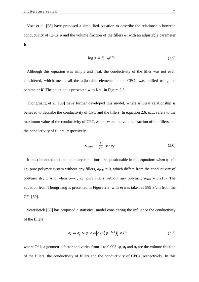
Voet et al. [58] have proposed a simplified equation to describe the relationship between
conductivity of CPCs σ and the volume fraction of the fillers φ, with an adjustable parameter
K:
log 𝜎 = 𝐾 ∙ 𝜑1/3 (2.5)
Although this equation was simple and neat, the conductivity of the filler was not even
considered, which means all the adjustable elements in the CPCs was unified using the
parameter K. The equation is presented with K=1 in Figure 2.3.
Thongruang et al. [59] have further developed this model, where a linear relationship is
believed to describe the conductivity of CPC and the fillers. In equation 2.6, σmax refers to the
maximum value of the conductivity of CPC. φ and σf are the volume fraction of the fillers and
the conductivity of fillers, respectively.
σ𝑚𝑎𝑥 =2
3𝜋∙ 𝜑 ∙ 𝜎𝑓 (2.6)
It must be noted that the boundary conditions are questionable in this equation: when φ→0,
i.e. pure polymer system without any fillers, σmax = 0, which differs from the conductivity of
polymer itself. And when φ→1, i.e. pure fillers without any polymer, σmax = 0.21σf. The
equation from Thongruang is presented in Figure 2.3, with σf was taken as 589 S/cm from the
CFs [69].
Scarisbrick [60] has proposed a statistical model considering the influence the conductivity
of the fillers:
𝜎𝑐 = 𝜎𝑓 × 𝜑 × 𝜑[𝑒𝑥𝑝(𝜑−2/3)] × 𝐶2 (2.7)
where C2 is a geometric factor and varies from 1 to 0.003. φ, σf and σc are the volume fraction
of the fillers, the conductivity of fillers and the conductivity of CPCs, respectively. In this

8 2 Literature review
equation, the conductivity of CPC can be more precisely predicted by adjusting the parameter
C2.However, the disadvantage of equation 2.7 is that the contribution of conductivity of
Polymer matrix was still not considered. The equation is presented with C2=1 and C2=0.003 in
Figure 2.3, with σf was taken as 589 S/cm from the CFs [69].
Sohi et al. [55] has proposed another model (equation 2.8) based on equation 2.7:
𝜎𝑐 = C × 𝜎𝑓 ×𝐴𝑅
10× 𝑆 × 𝜑 × 𝜑[𝑒𝑥𝑝(𝜑−2/3)] + (1 − 𝜑)𝜎𝑚 (2.8)
where fillers aspect ratio AR, and the conductivity of polymer matrix σm are considered. C is
the geometric factor and varies from 1 to 0.001. AR is the aspect ratio of the fillers and S is the
surface to volume ratio in μm-1. The equation 2.8 is presented with C=1 and C=0.001 in Figure
2.3, with σf =589 S/cm, and AR=100.
Bueche [61] has proposed a model, also considering the polymer matrix conductivity:
𝜎𝑐 = 𝜑 ∙ 𝜎𝑓 + (1 − 𝜑) ∙ 𝜎𝑚 (2.9)
where σc, σm and σf are the conductivities of the composite, the polymer matrix and the
conductive fillers, respectively. is the volume fraction of fillers. The conductivity of CPC is
thus considered as a sum of conductivity contribution from the polymer matrix and the
conductivity of fillers. The equation 2.9 is presented in Figure 2.3, with σf =589 S/cm.
Based on the model from Bueche (equation 2.9), McCullough [62] has added modified
components, which is more precise:
𝜎𝑐 = 𝜑𝜎𝑓 + (1 − 𝜑)𝜎𝑚 − [𝜑(1 − 𝜑)𝑆(𝜎𝑓 − 𝜎𝑚)2/(𝑉𝑓𝜎𝑓 + 𝑉𝑚𝜎𝑚)] (2.10)
V𝑓 = (1 − S) ∙ 𝜑 + S ∙ (1 − φ) (2.11)
2 Literature review 9
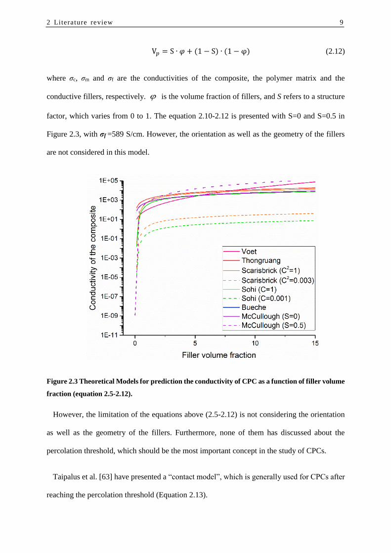
V𝑝 = S ∙ 𝜑 + (1 − S) ∙ (1 − φ) (2.12)
where σc, σm and σf are the conductivities of the composite, the polymer matrix and the
conductive fillers, respectively. is the volume fraction of fillers, and S refers to a structure
factor, which varies from 0 to 1. The equation 2.10-2.12 is presented with S=0 and S=0.5 in
Figure 2.3, with σf =589 S/cm. However, the orientation as well as the geometry of the fillers
are not considered in this model.
Figure 2.3 Theoretical Models for prediction the conductivity of CPC as a function of filler volume
fraction (equation 2.5-2.12).
However, the limitation of the equations above (2.5-2.12) is not considering the orientation
as well as the geometry of the fillers. Furthermore, none of them has discussed about the
percolation threshold, which should be the most important concept in the study of CPCs.
Taipalus et al. [63] have presented a “contact model”, which is generally used for CPCs after
reaching the percolation threshold (Equation 2.13).

10 2 Literature review
Xvd
dlff
cmc
)(
cos42
2
(2.13)
where σc, σm and σf are the conductivities of the composite, the polymer matrix and the
conductive fillers, respectively. d = diameter of the fibers, l = average length of the fibers, θ =
average angle between the inclination of fibers and the direction of the applied voltage, vf is the
volume fraction of the fillers, and X is a factor depending on the contact number of fibers, i.e.,
the vf. Finally, dc is the diameter of the circle of contact, which depends on the applied voltage
(Figure 2.4).
Figure 2.4 Schematic models of three different type of contact CFs in “contact model”: (a) a thin
layer of polymer is between two CFs ; (b) two CFs contact just on one single point; (c) a flat circle
of contact between CFs. [63]
In Equation 2.13, it must be noted that the diameter of the circle of contact dc has a direct
influence on the conductivity of CPCs, which can only be obtained by fitting the local data
points, and no comparative values can be found from literature. Therefore, Equation 2.13 is not
a suitable model to calculate the conductivity of composites, but is able to explain the
conductivity phenomena in a CPC.

2 Literature review 11
Mamunya et al. [64] has proposed a model, including the filler and polymer surface energies.
According to this model, the electrical conductivity of CPC is presented as follows:
log 𝜎𝑐 = log 𝜎𝑝ℎ𝑖_𝑐 + (log 𝜎𝑚𝑎𝑥 − log 𝜎𝑝ℎ𝑖_𝑐) × (𝜑−𝜑𝑐
𝐹−𝜑𝑐)𝑘
(2.14)
k = (A − B ∙ γ𝑝𝑓) ×𝜑𝑐
(𝜑−𝜑𝑐)0.75 (2.15)
γ𝑝𝑓 = γ𝑝 + γ𝑓 − 2(γ𝑝γ𝑓)0.5 (2.16)
𝐹 =5
75
10+𝐴𝑅+𝐴𝑅
(2.17)
where σc, σphi_c and σmax are the electrical conductivity of the composite, of the composite at the
percolation threshold, of the composite at maximum volume fraction of fillers, respectively. F
is the maximum volume fraction of the conducting filler, corresponds to the filler geometry
aspect ratio (AR). And if the filler is spherical (AR=1) F = 0.64, which corresponds to the sphere
close packing. γp and γf surface energies of polymer and fillers, respectively. A and B are two
parameters with A=0.11 and B=0.03. The limitation of this model is that the data points with
filler volume fraction below percolation threshold can not be used. Therefore, in this thesis,
model from Mamunya has not been applied to obtain the percolation threshold.
The most effective model is the general effective medium (GEM) equation presented by
McLachlan [67, 68]:
( 1 − 𝜑)𝜎𝑚1 𝑠⁄
−𝜎𝑐1 𝑠⁄
𝜎𝑚1 𝑠⁄
+(1−𝜑𝑐)/𝜑𝑐∙𝜎𝑐1 𝑠⁄ + 𝜑
𝜎𝑓1 𝑡⁄
−𝜎𝑐1 𝑡⁄
𝜎𝑓1 𝑡⁄
+(1−𝜑𝑐)/𝜑𝑐∙𝜎𝑐1 𝑡⁄ = 0 (2.18)
where σm, σc, σf are the conductivities of the PMMA matrix, the composite and the CFs,
respectively. The volume fraction of CFs is denoted 𝜑 and the percolation threshold 𝜑𝑐. For
3-D systems, the exponential factors are generally set to s = 0.87 and t = 2. The advantage of

12 2 Literature review
this model is that all the data points obtained from the experiment can be fitted using Mclachlan
model, and the percolation threshold can be thus obtained for further study.
2.3 Ternary conductive polymer composite
Conductive polymer composites (CPCs) have generated a great deal of interest due to its
high conductivity, low weight, and the ease of processing [70-73]. Besides CFs, Carbon
nanotubes (CNTs) and carbon black (CB) are two conductive fillers, which are also most
commonly used for the design of CPCs [74-79]. Recently, studies on the ternary CPCs
comprising CNTs and CB have been widely reported, because a combination of CB and CNTs
is a good way to improve the electrical properties while limiting the costs [80-88].
However, few theory has been developed for describing the conductivity of the ternary system.
A theoretical description [89] has been put forward to explain the synergistic effect. For a CPC
with a certain concentration of fillers i.e. aCFbCB, it can be assumed to be two resistors
(PMMA with a vol. % CF and PMMA with b vol. % CB) connected in parallel or series (Figure
2.5).
Figure 2.5 The resistance of PMMA/aligned CFs/CB composite filament considered as two
resistors - (a) parallel or (b) series connected.
(a) (b)

2 Literature review 13
The theoretical conductivity magnitudes, both should be lower than the experimental
conductivity, assuming series (Equation 2.19) or parallel (Equation 2.20) connections of
conductive CB and CF networks:
𝜎𝑝𝑎𝑟𝑎𝑙𝑙𝑒𝑙 =1
2(𝜎𝑃𝑀𝑀𝐴/𝐶𝐵 + 𝜎𝑃𝑀𝑀𝐴/𝐶𝐹) (2.19)
𝜎𝑠𝑒𝑟𝑖𝑒𝑠 = 2(𝜎𝑃𝑀𝑀𝐴/𝐶𝐵∙𝜎𝑃𝑀𝑀𝐴/𝐶𝐹
𝜎𝑃𝑀𝑀𝐴/𝐶𝐵+𝜎𝑃𝑀𝑀𝐴/𝐶𝐹) (2.20)
where σPMMA/CB, σPMMA/CF are the conductivities of composites with certain concentration of CB
only and CF only, respectively. The corresponding conductivity of PMMA/aligned CF and
PMMA/CB can be revealed from experiments. The conductivity values estimated by applying
this method can be thus compared with the experimental values. However, the conductivity of
binary composites (i.e. only one filler is used alone) cannot be obtained from equation 2.20,
which leads to a wrong conclusion from the boundary conditions.
Sun et al. [81] have proposed a percolation threshold model based on the assumption that the
excluded volume of the two fillers can be added together linearly. The percolation threshold of
a conductive composite with two fillers can then be predicted as:
KBc
B
Ac
A ,,
(2.21)
where φA and φB are the volume fractions of filler A and filler B in ternary composites,
respectively, while φc,A and φc,B are the corresponding percolation concentrations when filler A
or B is used alone in binary composites. When K=1, the percolation threshold is just reached.
When K>1 the fillers in the composites connect each other (i.e. the composites are conductive)
and when K<1 the composites are insulating. Based on this model, the potential synergic effects
between CFs and CB have been discussed [89], defining “synergy” as a lower percolation
threshold of the mixture than predicted by Eq.1 with K=1. It should be noted that, according to

14 2 Literature review
Eq. 1, a linear relationship between volume fractions φA and φB can be established once the
percolation thresholds φc,A and φc,B are determined.
In spite of this, for a ternary composites with CB and CNTs, a “synergistic effect” is still
widely used to indicate the enhancement of the conductivity [74-88] yet without unified clear
definition. Figure 2.5 is a typical schematic diagram for the “synergy”: the CNTs are considered
as 1-D filler with a large aspect ratio (AR), while CB are 0-D spherical particles. Therefore,
due to the geometry of both fillers, the electrical pathway was expected to be easier formed in
the CNTs/CB ternary CPCs than the binary CPCs with only one filler. Different morphological
structure was proposed to explain such phenomenon, such as “grape-like” [82, 85], or
“conductivity-bridge” [79, 83].
Figure 2.5 Schematic structure of ternary CPCs with CNTs and CB. (a) The well-known “synergy”
structure between CNTs and CB; (b) The well-dispersed CB particle in fact with the same volume
fraction; (c) A higher CB volume fraction is needed to achieve the “synergy” model in (a).
Unfortunately, there is still no clear definition on the “synergistic effect” on the conductivity
between CNT and CB. From the basic concept, it can only be assumed that this is an effect
shows 1+1˃2. Until now, there are three main perspectives to explain the “synergistic effect”
between CNT and CB:
1st synergy: A “small amount” of CNTs (or CB) (with either volume or weight percent) will
“dramatically” increase the conductivity of the CPCs [75, 76].
𝜎(𝜑𝐶𝑁𝑇𝑠)𝐶𝑁𝑇𝑠 < σ(𝜑𝐶𝑁𝑇𝑠, 𝜑𝐶𝐵)𝑡𝑒𝑟, with φCB<< φCNTs (2.22)
𝜎(𝜑𝐶𝐵)𝐶𝐵 < σ(𝜑𝐶𝑁𝑇𝑠, 𝜑𝐶𝐵)𝑡𝑒𝑟, with φCNTs<< φCB (2.23)

2 Literature review 15
2nd synergy: The conductivity of the ternary CPCs is higher than that of either binary CPCs,
while the total filler fraction keeps constant. Sometimes an optimal ratio between CNTs and
CB was presented. [77, 80, 82-86, 88]
𝜎(𝜑𝐶𝐵)𝐶𝐵 < σ(𝜑𝐶𝑁𝑇𝑠, 𝜑𝐶𝐵)𝑡𝑒𝑟 > 𝜎(𝜑𝐶𝑁𝑇𝑠)𝐶𝑁𝑇𝑠, with φCNTs+ φCB=constant (2.24)
3rd synergy: The experimental percolation threshold of ternary CPCs is lower than the
predicted one according to Equation 2.21, which is proposed for the situation when the
percolation threshold of ternary CPCs is just reached, and the predicted percolation threshold
of the ternary CPCs is defined as (φCNT+φCB). Usually, a certain ratio between CNT and CB
were used to produce the ternary composite. Once the percolation thresholds φc,CNT and φc,CB
are determined, then the predicted percolation threshold of the ternary CPCs can be calculated.
Based on this model, the 3rd synergic effects between CFs and CB have been widely discussed
[77, 78, 82-88].
2.4 Outline of the thesis
In this thesis, efforts have been made on the morphological and electrical behavior of
anisotropic filament from PMMA based conductive composites. In Chapter 2, the background
information as well as the models describing electrical conductivity of CPCs were presented.
In Chapter 3, the materials, the processing and characterization methods involved in this thesis
were introduced. In Chapter 4, the binary PMMA/CF composite filament have been studied, in
order to reveal the influence of (1) aspect ratio (AR) of fillers; (2) orientation of fillers on the
electrical conductivity of the CPCs. Besides the development of existing equation and theories
of electrical conductivities, a novel approach has been proposed to explain the counterintuitive
phenomenon. In Chapter 5, the ternary composite PMMA/CB/CF has been studied. Based on
a model for predicting the percolation threshold of ternary composites, a novel equation has
been proposed to predict the conductivity of ternary composites. In Chapter 6 ternary composite

16 2 Literature review
comprising PMMA/CB/CNTs has also been presented. A novel quantified definition
‘Synergasm’ was proposed, which is able to precisely describe the synergic effect between CB
and CNTs for the first time. The conclusion of this thesis is summarized in Chapter 7 and 8 (in
the language of German). Chapter 9 presents the additional information as supplementary
material for this work.

3 Experimental section
3.1 Materials
In this work, Poly(methyl methacylate) (PMMA) was chosen as the polymer matrix, due to
its high impact strength, lightweight and favorable processing conditions. Moreover, as an
amorphous thermoplastic polymer, the influence of the rare PMMA polymer crystallization on
filler distribution can be thus minimized and ignored. Commercial PMMA Plexiglas 7N was
obtained from Evonik Röhm GmbH, with a weight-average molar mass 𝑀𝑤 of 99 kg/mol, a
polydispersity index of 1.52, and a density 1.19 g/cm3.
The carbon fillers used in this work are carbon fibers (CF), carbon black (CB) and carbon
nanotubes (CNTs). The CF segments (Figure 3.1 (a)) were obtained from Tenax® - JHT C493
(Toho Tenax Europe GmbH, Wuppertal, Germany) with a diameter of 7 µm, an initial length
of 6 mm, a specific resistance of 1.7×10⁻³ Ω/cm, and a density 1.79 g/cm3. CB (Figure 3.1 (b))
was Printex XE2 from Evonik Degussa, with a specific surface area of 900 m2/g measured by
the BET-method. The mean diameter of the primary CB particles was around 35 nm and the
density at room temperature was 2.13 g/cm3. CNTs (Figure 3.1 (c)) were Bayertubes® C 150

18 3 Experimental section
P, with an outer diameter of 13 nm, an inner diameter of 4 nm, an average length of 1 µm and
a bulk density of 130-150 kg/m3.
Figure 3.1 Morphological photos of the carbon fillers used in this work: (a) carbon fibers; (b)
carbon black; (c) carbon nanotubes.
3.2 Composites preparation
3.2.1 1st step melt mixing process of binary composites and master batches
Prior to processing, all the materials in this study were dried 24 hours under vacuum at 80 ˚C.
The composites were produced by melt mixing procedure in an internal kneader PolyDrive
(Haake, 557-8310) (Schwerte, Germany) at a temperature of 200 ˚C and a rotation speed of 60
rpm. The melt mixing recipe is presented in Figure 3.2, where the binary composites system
PMMA/CF (Figure 3.2 (a), blue circle), PMMA/CB (Figure 3.2 (b), black circle) and
PMMA/CNTs (Figure 3.2 (c), red circle) were prepared.
The PMMA and the corresponding carbon fillers were simultaneously fed into the kneader
and mixed for 10 minutes. Parts of carbon fillers were found to be stuck in the gap of the
machine (especially with high concentration of CF). These fillers were not participated in the
melt mixing procedure and were therefore manually removed. The remaining composites were
mixed for another 10 min under the same conditions. The binary PMMA/CF composites were
produced with 10-60 vol. % CF, the binary PMMA/CB composites were produced with 1-20

3 Experimental section 19
vol. % CB, and the binary PMMA/CNTs composites were produced with 0.01-30 vol. % CNTs.
The composites, with 40 vol. % CFs, 50 vol. % CFs 60 vol. % CFs and 20 vol. % CB were
named as master batches (MB) and marked with bold circle. Therefore, this process was named
as 1st step melt mixing process, because only binary composites system and MB composites
were produced in this procedure. The following nomenclature is used for the samples: 50CF
means that the expected concentration of CF was 50 vol. %, 20CB means that the expected
concentration of CB was 20 vol. %, created by the 1st-step mixing process. After melt mixing,
all the composites were ground into granules and dried under vacuum at 80 ˚C for 24h.
Figure 3.2 Process flow chart of the 1st step melt mixing method. (a) PMMA/CF binary composites,
those which concentration were 40 vol.%, 50 vol.% and 60 vol.% CFs are used as master batches
for further dilution; (b) PMMA/CB binary composites, those which concentration were 20 vol.%
CB are used as master batches for further dilution; (c) PMMA/CNT binary composites.
3.2.2 2nd step mixing process for AR control and ternary composites system
Composites with concentrations of 40, 50 and 60 vol. % CFs from 1st-step mixing were treated
as master batches (MB), and portions of these batches were further diluted with pure PMMA
to the required concentration (2nd-step mixing), as illustrated in Figure 3.3 (a). The following
nomenclature is used for the samples, which will be discussed in Chapter 4: 10(-50)CF means

20 3 Experimental section
that the composite from 2nd-mixing with an expected CF concentration of 10 vol. % was
obtained by dilution of the master batches 50CF. Using this two-step mixing procedure, the
length or the aspect ratio (AR) of CFs can be controlled, as presented by Starý et al. [23].
The PMMA/CB/CF ternary composites were produced by diluting the mater batches 50CF
with pure PMMA and CB to the required concentration (Figure 3.3 (b)), which will be discussed
in Chapter 5. The following nomenclature is used for the samples: aCB and bCF denote the
composites with a % volume fraction of CB, and b % volume fraction of CFs, respectively.
Thus, the sample with the name aCBbCF presents the ternary composite filled with a vol. %
CB and b vol. % CFs and (100-a-b) vol. % PMMA. In this study, a ∈ [0, 20], and b ∈ [0,
50].
The PMMA/CB/CNTs ternary composites were obtained by diluting the mater batches 20CB
with pure PMMA and CNTs to the required concentration (Figure 3.3 (c)), which will be
discussed in Chapter 6. The following nomenclature is used for the samples: mCB and nCNTs
denote the composites with m % volume fraction of CB, and n % volume fraction of CNTs,
respectively. Thus, the sample with the name mCBnCNTs presents the ternary composite filled
with m vol. % CB and n vol. % CNTs and (100-m-n) vol. % PMMA. In this study, m ∈ [0,
20], and n ∈ [0, 30].
After melt mixing, all the composites were ground into granules and dried under vacuum at
80 ˚C for 24h.

3 Experimental section 21
Figure 3.3 Process flow chart of the 2nd step melt mixing method. (a) Using the MB from 1st step
mixing process, the length of CFs can be controlled in the produced composites; (b)
PMMA/CB/CF ternary composites were produced by diluting the MB (50CF) with CB and pure
PMMA; (c) PMMA/CB/CNTs ternary composites were produced by diluting the MB (20CB) with
CNT and pure PMMA.
3.3 Extrusion process
The composite granules after drying were anisotropic at 200 °C utilizing a capillary
rheometer (Göttfert, Rheograph 2003), (Göttfert, Buchen, Germany), using either a 10-mm
length die with a diameter D = 1 mm or a 10-mm length die with a diameter D = 3 mm. A
constant extrusion speed v = 0.08 mm/s of the pistol (with diameter D0 = 12 mm) was applied
using both dies. Therefore, the apparent shear rate of the anisotropic composite filaments can
be calculated from Equation 3.1 [107], resulting in (D = 1 mm) = 92.16 s−1, and (D = 3
mm) = 3.41 s−1.
=8∙𝑣∙𝐷0
2
𝐷3 (3.1)

22 3 Experimental section
Figure 3.4 The anisotropic PMMA composites using 3 mm die and 1 mm die.
The samples with 3 mm diameter will only be discussed in Chapter 4.6.1 and 4.6.3, while
the samples with 1 mm diameter will be discussed in all the chapters.
3.4 Thermogravimetric analysis (TGA)
The resulting CF concentrations of the composite filament were determined by
thermogravimetric analysis (TGA 2950, TA Instruments). Ca. 20-30 mg samples from the
corresponding CPCs were heated from room temperature to 600 ˚C with a heating rate of
10 °C/min under a nitrogen atmosphere.
3.5 Morphology
3.5.1 Investigation on CFs length distribution
In order to determine the CF length distributions in the composites, the PMMA/CF binary
composite filament were handled with acetone. PMMA matrix was dissolved and the CFs were
investigated using a light microscope (Leitz, Orthoplan P). The images obtained were then
analyzed using the JMicrovision image analysis software. At least 500 carbon fibers per
concentration were studied and measured.

3 Experimental section 23
3.5.2 Investigation on the orientation and distribution of CFs
In order to study the orientation of CFs inside the composite filaments, the composite
filaments were circle peeled (annular cut) (Figure 3.5, (a)), and ultrasonic washing with ethanol.
The samples were then observed with a light microscope, and the orientations of CFs on the
surface and inside were compared at the same time. The composite filament were also fixed
with epoxy resin. The epoxy resin as well the composite were then polished, until the width of
the exposed surface of the composite was equal to the original diameter of the composite
filament. (Figure 3.5, (b)). With the light microscope, 500 carbon fibers (for the 1 mm diameter
composite filament) or 1200 carbon fibers (for the 3 mm diameter composite filament) were
randomly chosen and the inclination between each carbon fibers and the extrusion direction can
be recorded and then analyzed with JMicrovision and Matlab software.
Figure 3.5 Two approaches to assess the orientation of CFs inside the anisotropic composite; (a)
circle peeling, in order to compare the CFs on the surface and with those inside the composites;
(b) polishing, in order to obtain the statistical distribution of the CFs.
3.5.3 Morphological observation of the carbon fillers
The morphologies of the composites were studied by a scanning electron microscope (SEM).
The anisotropic samples were fractured in liquid nitrogen and the broken surfaces (cross section
or the middle section as presented in Figure 3.5 (b)) were sputtered with a thin layer of

24 3 Experimental section
palladium, were then analyzed using a SEM (Leica, LEO 435VP) equipped with a secondary
electron detector at an acceleration voltage of 10KV.
3.6 Electrical conductivity measurement
3.6.1 Vertical conductivity measurement
Since anisotropic the CPCs filaments were anisotropic, the electrical conductivity
measurement were carried out in two directions, in order to check the influence of the measuring
direction, i.e. the direction of the applied voltage on the conductivity of the CPCs. The vertical
measurement refers to a parallel relationship between the extrusion direction of the CPCs
samples and the applied voltage, and this measurement is used for discussion for all the chapters
in this study. The composite filament were cut into samples of 20 mm length and their end-
sections were polished in order to remove isolate polymer. Silver conductive paste was then
coated (exclusively) at the polished ends, to ensure enough contact between the samples and
the copper electrode, as shown in Figure 3.6.
Figure 3.6 Schematic of silver coated sample for the vertical conductivity measurement.
The electrical resistance R of the samples at room temperature was measured using a Keithley
6487 Pico ammeter (Tektronix, Beaverton, United States) at a constant voltage 1 V. The volume
conductivity σ was calculated as follows:
RD
L
2
4
(3.2)

3 Experimental section 25
where R is the electrical resistance of the composite, L is the distance between two silver-coated
ends of the sample, and D is the diameter of the composite filament. Because the diameters of
the extrudes samples were close to the diameters of the extrusion dies (1 mm and 3 mm), a
slight reduction of the fiber diameter of less than 5% was observed as a consequence of
stretching during fiber spinning by gravity. A Vernier caliper was used for the diameter
measurements on the samples. For each material composition, 20 composite samples were
manufactured and analyzed for the conductivity measurement. Each presented conductivity
data point in this study is thus the average of 20 individual measurements on different samples.
It must be noted that the room temperature, as well as the humidity in the air, has an influence
on the conductivity of the anisotropic sample and the measured values. Therefore, the
conductivity of pure PMMA have been determined for each different set of the experiment. The
pure PMMA fiber have been anisotropic and measured, using the same conditions as the other
composites.
3.6.2 Horizontal conductivity measurement
The horizontal measurement refers to a perpendicular relationship between the extrusion
direction of the CPCs samples and the applied voltage, and the results based on this
measurement is discussed in Chapter 4.6.1. The samples with 3 mm diameter were set into
epoxy resin, and polished on both side surface, until the exposed width of CPCs on the both
ends equal to required W. The surface of the sample were then coated with silver and measured.

26 3 Experimental section
Figure 3.6 Schematic of silver coated sample for the horizontal conductivity measurement.
The horizontal conductivity of the anisotropic filament can be thus determined using :
𝜎 =ℎ
𝐿∙𝑊∙𝑅 (3.3)
where R is the electrical resistance of the composite, L is the length of the sample, h is the
height of the epoxy resin, and W is the width of the sample. A rough estimation is proposed to
obtain the horizontal conductivity, which is presented in Chapter 9.1.
A Vernier caliper was used for the measurements on W and h. For each material composition,
3 composite samples were manufactured, polished to different W, and analyzed. Each presented
conductivity data point is thus the average of 3 individual measurements on different samples.

4 PMMA/CF binary system

28 4 PMMA/CF binary system
4.1 Introduction
Carbon fibers (CFs) are widely used as conductive fillers, and have gained increasing
attention in both academic and engineering aspects [15-25]. With plate-shaped [16], cuboid [15,
89] or even composite films [17], most of literature has discussed the effect of CFs with a
maximum concentration of 10 vol. %, because this is already above the percolation threshold
of CPCs with isotropic CFs, after which there is no significant change in the electrical properties
of the composites (Figure 2.3). In this study, the volume fraction of CFs in the CPCs were
achieved up to 60 vol.% (Chapter 4.2), in order to present a general investigation on the
electrical properties of the PMMA/CF system.
Besides the volume fraction, the aspect ratio (AR) of CFs has also a dramatically influence
on the percolation threshold of the CPCs [23, 97-99]. It has been reported that the percolation
threshold of the CPCs is approximately proportional to the reciprocal of the aspect ratio (AR-1)
of the fillers. In this study, CF aspect ratios were controlled by using a two-step melt mixing
method (Chapter 4.4), the influence of the carbon fibers’ AR on the electrical properties is
presented in Chapter 4.6.2.
Moreover, it has also been reported that the threshold of the composite also depends on the
orientation of the CFs [8, 9]. With a higher orientation of CFs, the percolation threshold is
shifted towards a higher volume fraction of fillers. Unlike CB (dot-like, 0-dimensional
particles), CFs with a high aspect ratio (AR) should be considered as 1-dimensional particles.
Due to the shear deformation during the extrusion process, the orientation of 1-D particles can
be induced. Another typical 1-D conductive filler, CNTs, however, due to the irregular shape
(fold, spiral) and much smaller scale compared to CFs, are not chosen and analyzed in this
chapter. In the past few decades, extensive efforts have been generally focused on polymer/CFs
composites with isotropic CFs. To our knowledge, polymer/CFs composites with highly

4 PMMA/CF binary system 29
anisotropic CFs has been rarely reported in the open literature. Therefore in this chapter,
composite with different CFs concentrations were anisotropic into composite filament with two
different diameters using a capillary rheometer, to induce CF orientation. The morphology on
the anisotropic PMMA/CF CPCs is shown as a “fibers in fiber” structure in Chapter 4.3. The
distribution of CF orientation in the CPCs is investigated and presented in Chapter 4.5 and the
influence of the fillers orientation on the electrical properties of PMMA/CF CPCs is discussed
in Chapter 4.6.3.
4.2 Thermogravimetric analysis (TGA) of the PMMA/CF composites
In order to determine the actual CF volume fractions in the PMMA/CF composites from the
designed CF volume fraction, the composites filament were tested by TGA measurements.
Composites from the 1st step melt mixing with five different designed CFs fractions (10; 20; 30;
40; 50; 60 vol. %) as presented in Figure 4.1. Since the actual CF weight fractions in the
composites were given as results from TGA, thus the corresponding actual CF volume fractions
can be calculated by Equation 4.1,
PMMACF
CF
wtwt
wtvol
/.%)1(/.%
/.%.%
(4.1)
where ρCF = 1.79 g/cm3 and ρPMMA = 1.19 g/cm3. The processing parameters (T = 200 °C,
extrusion speed of pistol = 0.08 mm/s) during the extrusion process has been optimized for
PMMA/CF composites, in order to get the smooth and uniform filament composite. Because of
the non-uniform distribution of CFs in the PMMA matrix, the TGA results could be difference
on samples even from the same extrusion process. Therefore, Figure 4.1 presents a certificate
of the difference between the actual CF concentration in the composites and the designed CF
concentration. This is because parts of CFs were lost and removed during the melt mixing

30 4 PMMA/CF binary system
process. These differences are indicated with error bars on the volume fraction of CFs in this
study.
Figure 4.1 The actual weight fraction and actual CFs volume fraction in the samples from 1st step
melt mixing. A difference between actual and designed CFs volume fraction can be found.
4.3 Morphological study of the anisotropic PMMA/CF composite filament
The morphology of the anisotropic PMMA/CF composite filament with 1 mm diameter is
investigated. The cross sections of composite filament with different concentration of CFs are
shown in Figure 4.2 (a) and (b). The CFs can be seen inside the composite filament, as well as
lots of "black holes", which indicate the positions of pulled out CFs. It should be noted that
almost all the CFs and the "black holes" are basically perpendicular to the cross section, i.e.
parallel to the axis of the composite filament (the extrusion direction). The red circle in Figure
4.2 (a) presents an exception, which shows the situation when a single CF is not parallel to the
axis of the composite filament, but this situation was rarely observed in our work.

4 PMMA/CF binary system 31
Figure 4.2. Cross sections of composite filament, different concentrations of CFs: (a) = 19.09
vol. %, (b) = 36.30 vol. %, one-step mixing. Red circles: a single CF is not parallel to the axis of
the composite filament.
The amount of PMMA matrix among the CFs is significant in Figure 4.2 (a). The CFs are
rarely connected, even when the concentration of CFs reaches almost 20 vol. %. As the
concentration of CFs increases, the agglomeration of CFs can be seen as in Figure 4.2 (b) with
the 36.3 vol. % CF. It is generally considered, the conductivity of the composites depends on
the amount of "conductive pathway", which are built up by the connection of CFs with each
other. From this point of view, it can be assumed that the composite in Figure 4.2 (b) is
conductive, while that in Figure 4.2 (a) is not. The conductive data are presented in Chapter
4.6.

32 4 PMMA/CF binary system
Figure 4.3 Schematic view of the orientation of CFs inside the composites; (a) due to the different
shear deformation of the composite melt, CFs have different orientations in different regions of
the composites; (b) schematic view of the composite, with different orientations of CFs in different
regions.
The flow pattern of the composite melt inside the capillary rheometer is shown as Figure 4.3
(a). The composite melt near the wall of the capillary (rim area marked dark grey) is subject to
higher shear deformation than the peripheral composite melt in the middle capillary (center area
marked light grey). After extrusion, the isotropic CFs (red segments) at first are differently
oriented due to the shear gradient across the channel section of the composites cylinder. Based
on this, the 3-D schematic view of the anisotropic composite filament with CFs is presented in
Figure 4.3 (b). The small white cylinders denote carbon fibers, the light grey and dark grey
parts denote the PMMA matrix, with lower (center part) and higher (rim part) shear deformation,
respectively. The CFs in the outer part of the composite are highly anisotropic along the axis of
the composite, i.e. the extrusion direction, while those in interior of the composite are less
oriented.
4 PMMA/CF binary system 33
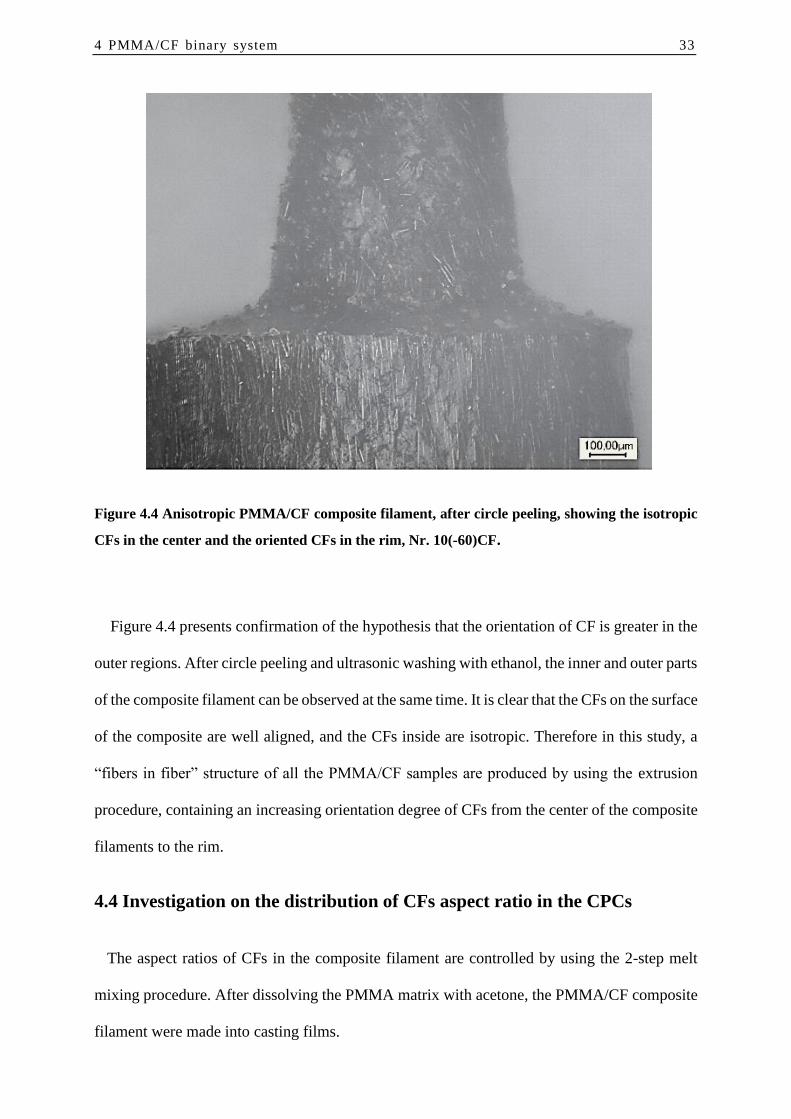
Figure 4.4 Anisotropic PMMA/CF composite filament, after circle peeling, showing the isotropic
CFs in the center and the oriented CFs in the rim, Nr. 10(-60)CF.
Figure 4.4 presents confirmation of the hypothesis that the orientation of CF is greater in the
outer regions. After circle peeling and ultrasonic washing with ethanol, the inner and outer parts
of the composite filament can be observed at the same time. It is clear that the CFs on the surface
of the composite are well aligned, and the CFs inside are isotropic. Therefore in this study, a
“fibers in fiber” structure of all the PMMA/CF samples are produced by using the extrusion
procedure, containing an increasing orientation degree of CFs from the center of the composite
filaments to the rim.
4.4 Investigation on the distribution of CFs aspect ratio in the CPCs
The aspect ratios of CFs in the composite filament are controlled by using the 2-step melt
mixing procedure. After dissolving the PMMA matrix with acetone, the PMMA/CF composite
filament were made into casting films.

34 4 PMMA/CF binary system
Figure 4.5 Length and distribution of CFs in the composites: (a) and (d)-Sample 10CF; (b) and
(e)-Sample 20CF; (c) and (f)-Sample 50CF.
In the cast films of the composites, the lengths of the CFs were able to be directly observed
under a microscope (Figure 4.5 (a)-(c)). The uncertainty "Δ" of the average "m" was estimated
as:
∆= ±1.96×𝑆𝐷
√𝑁 (4.2)
N is the number of units studied, equal to 500 in this work, and SD is the standard deviation,
which means that the true mean µ is with 95% confidence in the range m ± Δ [96]. Figure 4.5
(d-f) shows the frequency distributions of the lengths of CFs in Figure 4.5 (a-c), respectively.
The results show that: the length of CFs after melt mixing decreased when the concentration of
CFs was increased. Presumably because the probability of CF collision under the melt viscosity
of composites with a higher CF content is increased, i. e. a higher CFs concentration of the
composite melt presents a higher viscosity, which leads to shorter CFs in the composite melt.
The average length of CFs was not changed by dilution from the master batches with pure
PMMA in the second step, as has been shown by Starý et al. [23]. The lengths of CFs in all the

4 PMMA/CF binary system 35
composites in this study, with different concentration of CFs, are present in Figure 4.6, which
shows that different aspect ratio of CFs (6.3, 9.2 and 12.0) were achieved. A possible model
describing the relationship between the average value of CFs and the volume fraction of CFs is
left for future study.
Figure 4.6 The average length of the CFs as a function of the volume fraction.
4.5 Investigation on the orientation of CFs in the CPCs
Johannsen et al. [100] has reported similar anisotropic PMMA/CNTs “fibers in fiber”
structure, where a lower concentration of CNTs in the boundary layer of the composite
filaments is found compared to the center, due to the extrusion swell effect. However in this
study, hardly any expansion of PMMA/CF composite after leaving the nozzle were observed.
Presumably because the properties of PMMA polymer matrix as well as the high concentration

36 4 PMMA/CF binary system
of CFs contributes to a negative extrusion swell effect. Therefore, only the orientation of CFs
in different region of the composite filament are discussed.
In order to investigate the statistical distribution of the CF orientation, the composites were
set in epoxy resin and polished. Figure 4.7 shows a section through the middle axis of the sample
with 1mm diameter under a microscope. The inner and outer parts of the composite are roughly
divided by two red lines. The CFs in the outer region are relative highly anisotropic, whereas
these in the inner region have a significant inclination. 500 CFs were randomly chosen from
the picture and their inclinations were determined. The mean value of the two borderlines (i.e.
the axis of the composite, or the extrusion direction) was defined as 0°, and the orientation of
the CFs with respect to this line were in a range of [-90°, 90°]. The frequency distribution of
the inclination is shown as illustration at bottom left in Figure 4.7. It should be noted that these
angles of inclination are taken from a two-dimensional image, which differs from the real
circumstance in a 3-D system. This method in this work thus provides only a rough estimate of
the distribution.
Figure 4.7 The middle section of the 1mm diameter anisotropic PMMA/CF fiber, with the
frequency distribution of the angles between the CFs and the axis of the composite filament, with
Nr. 60CF.

4 PMMA/CF binary system 37
Figure 4.8 (a) presents the investigation on the inclinations of 500 CFs in an anisotropic
composite filament with 1 mm diameter. The randomly chosen CFs are marked with red
segments. The inclination between each CF segment and the borderlines of the composite
filament is presented in Figure 4.8 (b), where 500 data points are presented in an X-axis range
of [-r, r] (r is the radius of the polished composite filament). Divide the data points into 20
intervals based on their X-values [-r, -0.9r); [-0.9r, -0.8r); …[0.9r, r], and calculate their mean
value of the inclinations. Thus the 500 data points can be concluded into 20 points (Figure 4.8
(c)) and a significant curve can be estimated. This is highly related to the stress distribution
across the section of pipe, where fluid flows through [101-104]. This section can be further
carried out and verified by Finite Element Analysis (FEM), which is left for future study, and
will not be discussed in this thesis.
Figure 4.8 Investigation on the distribution of CFs. (a) polished PMMA/CF sample and the 500
CFs marked as red segments; (b) the radical position of CFs and the inclination of each CF; (c)
divide X-axis into 20 interval, the mean value of the inclination and the fitted curve, consists with
the shear stress distribution diagram of a pipe in pipeline hydrodynamics.
In this study, <sin γ> is used to describe the orientation of CFs in the composite filament [65,
66]. <sin γ> is the average sinusoidal value of the angle γ between each pair of CFs in the
system:

38 4 PMMA/CF binary system
< sin 𝛾 >=∑ ∑ 𝑠𝑖𝑛|𝜃𝑖−𝜃𝑗|
𝑖−1𝑗=1
n𝑖=1
∑ 𝑖n−1𝑖=0
(4.3)
where n=500 for the 1 mm diameter samples, and n=1200 for the 3 mm diameter samples. <sin
γ> was obtained with Matlab software, and is used in a discussion of excluded volume theory
in Chapter 4.6.2. The results of the samples with 1 mm diameter (plain segments) and 3 mm
diameter (shadowed segments) are shown in Figure 4.9, where CFs with AR≈12, 9 and 6 are
shown in black, red and blue respectively. The value <sin γ> of composite filament with each
volume fraction and each CFs AR is presented in three parts: the upper value refers to the <sin
γ> obtained from CFs in inner region of the composite filament (Figure 4.7), the lower refers
to data from outer region of the composite filament (Figure 4.7), and the middle value is the
average.
Figure 4.9 The orientation of CFs <sin γ> vs. volume fraction of CFs, considering different
CFs AR and different diameters of the composite filament.
It can been estimated that either the longer CFs or the higher concentration of CFs, contributes
to a smaller <sin γ>, i.e. to a greater orientation of CFs, presumably because either the longer
CFs or the higher concentration of CFs enhances the viscosity of the composite melt [23]. When

4 PMMA/CF binary system 39
the composite melt flows in the capillary rheometer, the composite melt with higher viscosity
develops more shear stress, which leads to a greater orientation of the CFs, i.e. a smaller value
of <sin γ>.
Moreover, the shear rate of the composite filament during the extrusion process also
influences the orientation of the CFs. For a system with totally aligned cylinders, when the
shear rate tends to infinity, <sin γ>=0. For a system with isotropic cylinders, when the shear
rate equals to zero:
< 𝑠𝑖𝑛𝛾 >𝑖𝑠𝑜=
∫ 𝑠𝑖𝑛 𝛾 𝑑𝛾𝜋0
∫ 𝑑𝛾𝜋0
=2
𝜋≈ 0.64 (𝑓𝑜𝑟 2𝐷 𝑠𝑦𝑠𝑡𝑒𝑚)
∫ 𝑠𝑖𝑛 𝛾∙𝑠𝑖𝑛 𝛾 𝑑𝛾𝜋0
∫ 𝑠𝑖𝑛 𝛾 𝑑𝛾𝜋0
=𝜋
4≈ 0.785 (𝑓𝑜𝑟 3𝐷 𝑠𝑦𝑠𝑡𝑒𝑚)
(4.4)
Therefore, considering these two boundary conditions, a model from Prof. Schubert is
suggested to describe the relationship between the <sin γ> and the shear rate :
< sin γ >=< 𝑠𝑖𝑛𝛾 >𝑖𝑠𝑜× (1−𝐵
1+(/𝐴)2+ 𝐵) (4.5)
where A and B are two adjustable parameters. Discussion on the relationship and model in
details is left for further study in the future.
Fig. 4.10 (a) shows the middle section of a cylindrical 3 mm PMMA/CF filament with 35
vol. % CFs. The figure is intended as an illustration of how the CF-orientation is determined in
this study and the sample is polished as presented in Fig. 3.5. The CFs can be seen as bright
segments in the micrograph. 1200 CFs were randomly chosen from the picture and the
inclination between each CF and the extrusion direction were determined (Fig. 4.10 (b)),
resulting in an averaged inclination angle θ which can be inserted in Eq. 2.13. The marked areas
A (red), B (green), C (blue) and D (purple) in Fig. 4.10 (b) correspond to the assumed structure
in Fig. 4.11 and Fig. 4.12. It should be noted that these inclination angles are taken from a two-

40 4 PMMA/CF binary system
dimensional (2-D) image, which differs from the real circumstance in a 3-D system, however
in the chosen plane this effect is negligible. Due to the shear gradient across the channel section,
the average angle between the CFs and the extrusion direction decreases from the outer part of
the composite to the center. The CFs in the center part of the composite cylinder are thus less
oriented. Moreover, the scattering in the CF orientation (Fig. 4.10 (b)) is symmetric around the
center due to axisymmetric geometry (r=0), resulting in a uniform CF-orientation distribution
in the extruded filament samples. The 1200 data points in Fig. 4.10 (b) are subsequently divided
into 15 intervals according to the X-position, and the average value of absolute CFs inclination
as a function of distance from the center axis is presented is Fig. 4.10 (c), which consists with
the shear stress distribution in the capillary

4 PMMA/CF binary system 41
Fig. 4.10 (a) The middle section of the 3mm diameter anisotropic PMMA/CF filament with 35
vol. % CF. (b) The 1200 CFs inclination vs. radical position of the sample. (c) Average value of
absolute CFs inclination as a function of the CF distance from the center axis.
Measured CF-orientations <cos2θ˃ were gathered for 6 different CF vol. % and 4 different
radial positions (layers A-D) in Tab. 4.1. The CF-orientation is generally reduced from the rim
part (A) to the center part (D), indicating that these regions were subject to a corresponding
decreasing shear stress during the extrusion process.
Tab. 4.1 The average orientation of CFs <cos2θ˃ in the different position of the 3 mm diameter anisotropic
PMMA/CF filament with different CFs concentration.
Region 𝒄𝒐𝒔𝟐𝜽
10 vol. % 20 vol.% 30 vol. % 35 vol. % 40 vol. % 50 vol. %
A (red) 0.991 0.989 0.988 0.990 0.987 0.943
B (green) 0.984 0.988 0.982 0.983 0.980 0.979
C (blue) 0.988 0.986 0.966 0.983 0.976 0.967
D (purple) 0.985 0.964 0.978 0.954 0.947 0.938
4.6 Electrical conductivity of the PMMA/CF binary composites
4.6.1 Anisotropic electrical conductivity of the 3mm diameter composite filament.
As known, the fillers orientation has a dramatic influence on the electrical conductivity of
CPC. Therefore, the electrical conductivity of the composite filament with aligned CFs should
be divided as vertical conductivity σV or σ∥ (parallel relationship between applied voltage and
extrusion direction) or σL (longitudinal conductivity) and horizontal conductivity σH or σ⊥
(perpendicular relationship between applied voltage and extrusion direction) or σT (transverse
conductivity). Moreover, due to the shear gradient across the channel section, the CFs

42 4 PMMA/CF binary system
orientation were decreased from the outer part of the composite to the center, which leads to
different conductivity in the radial direction of the composites filament, i.e. the value of <sin γ>
increases from the outer region of the composite filament to the inner region of that. Thus, in
order to investigate the vertical conductivity σV and the σH, the different composition, i.e. the
non-uniform orientation of CFs in the CPCs must be taken into consideration.
A CPC filament with a radially uniform filler fraction, which is assumed in this study, can be
modeled as a resistor network (Fig. 4.11 (a)). A filament for example consisting of two radially
separated material layers (i.e. one inner region and one outer region) can be represented by the
resistor network of Fig. 4.11 (b), where the colors of the resistors (red, blue, green) indicate
different resistance values. The radial (green) resistors are neglectable for the conductivity,
which means that the CPC filaments of this study can be modeled as resistive networks with
four (non-connected) concentric cylinders (Fig. 4.11 (c)). The electrical properties of the CPCs
were (among others) analyzed using this model.
Fig. 4.11 The assumed structure of a CPC filament in this study. (a) A simple resistor network
mimicking a filament with radially independent conductivity; (b) A resistor network with two
concentric layers, connected radially with green resistors; (c) a resistor network with four
concentric layers, where the radial resistors were omitted.
4.6.1.1 Analysis on the longitude conductivity σ∥

4 PMMA/CF binary system 43
In order to investigate the conductivity of each layer, the filament was considered as four
concentric circles at first, with same resistivity in each region (Figure 4.12 (a)). A “peeling-off”
procedure was applied for the investigation of the vertical conductivity σV or σ∥ of filaments.
At first, the conductivity of samples with certain length was measured at the original status
(Figure 4.12 (a)). Afterward, the sample was circle peeled to the expected radius (annular cut,
Figure 4.12 (b) to (d)), to remove the outer composites and then ultrasonic washed with ethanol
and dried for 24 hours. Both ends of samples were coated with silver for the conductivity
measurement (Chapter 3.6.1). Therefore, for each concentration of composites, four vertical
resistance (Rv,a- Rv,d) were obtained.
Figure 4.12 “peeling-off” procedure to obtain the longitudinal resistivity of the different regions
from the CPC filament. (a) Original extruded filament with 1.5 mm radius; (b) peeled-off filament
with 1.2 mm radius; (c) peeled-off filament with 1.0 mm radius; (d) peeled-off filament with 0.9
mm radius. The light-colored discs at the bottom only indicate the original geometry of the
filament.
The next objective was thus to convert the (global) resistance data to the (local) conductivities
of the concentric filament layers. It was observed that the geometry of Fig. 4c can be considered
as a parallel coupling (resistivity RL,c) between the blue cylindrical shell (resistivity RL,blue) and
the purple solid cylinder (resistivity RL,d). Since the longitudinal resistances RL,c and RL,d are
known, the unknown RL,blue of the blue shell can be calculated from:
1
𝑅𝐿,𝑐=
1
𝑅𝐿,𝑏𝑙𝑢𝑒+
1
𝑅𝐿,𝑑 (4.6)

44 4 PMMA/CF binary system
The same procedure was used to calculate the resistances RL,green and RL,red for the green and
red cylindrical shells. Since the dimensions of the four cylinders were known, the longitudinal
electrical conductivity of each region σ∥, A (red region), σ∥, B (green region) σ∥, C (blue region)
and σ∥, D (purple region) from the 3 mm filament could thus be calculated. The conductivity σ
was calculated as follows:
𝜎 =𝐿
𝑆∙𝑅 (4.7)
where L is the length of the sample, S is the area of the sample, and R is the corresponding
resistance.
4.6.1.2 Analysis on the longitude conductivity σ⊥
In addition, a “polishing” procedure was applied for the investigation of the horizontal
conductivity σH or σ⊥ of filaments. The samples were set into epoxy resin and polished till the
targeted width is exposed (Figure 4.13, from (a) to (d)). The sample was then ultrasonic washed
with ethanol and dried for 24 hours. Both sides of samples were coated with silver for the
conductivity measurement (Chapter 3.6.2). Therefore, for each concentration of composites,
four horizontal resistances (RH,a- RH,d) were obtained for further calculation.

4 PMMA/CF binary system 45
Figure 4.13 A four-step polishing procedure for obtaining the local transversal conductivites of a
CPC filament. Each filament is polished until the desired width (W) of the exposed sample is
reached. (a) Wa=1 mm, (b) Wb=1.8 mm, (c) Wc=2.2 mm, (d) Wd=2.4 mm.
In order to determine the transversal volume resistance (RT) in the horizontal direction, the
samples have been polished as presented in Fig. 4.13. Since the length of the investigated
samples in Fig. 4.13 always remain the same, therefore, only the cross section of the samples
are presented in this section for a better understanding. The four cross sections of the sample
(with four different polished width WA, WB, WC, WD), as well as the four corresponding
measured resistances RT,a, RT,b, RT,c, RT,d are presented in Fig. 4.14 (a). Four concentric circles
are assumed, with a constant resistivity ρ1, ρ2, ρ3 and ρ4 in each region (red, green, blue and
purple, respectively). This section presents the strategy on calculating the resistivity ρ1-ρ4 from
the experimental resistances RT,a -RT,d.
Fig. 4.14 (a) Collection of four cross sections of the sample from Fig. 4.13. (b) A rough assumption
on the resistance, based on a series connection, to calculate R1.
The applied voltage direction is given along the Y-axis, thus the measured resistance RT,a is
roughly considered as a series connection between the resistors in Fig. 4.14(b) -(c). Therefore,
the resistance of the shadowed area R1:

46 4 PMMA/CF binary system
𝑅1 =𝑅𝑇,𝑎−𝑅𝑇,𝑏
2≅ ∫
𝜌1
𝑊(𝑦)∙𝐿
𝑦1
𝑦2𝑑𝑦 (4.8)
where W(y) is the width of the sample at the position y, L is the length of the sample as presented
in Fig. 4.14. Thus, the resistivity ρ1 can be obtained.
Similarly, the resistance of structure R2 presented in Fig. 4.15 (a) is given by:
𝑅2 ≅𝑅𝑇,𝑏−𝑅𝑇,𝑐
2 (4.9)
Fig. 4.15 (a) The resistor R2 and the corresponding structure. (b) A rough assumption of the
resistor R2 based on a parallel connection. (c) A rough estimation on the resistance of RR, based
on a series connection.
which is further assumed as a parallel connection between RL (left), RC (center) and RR (right),
as presented in Fig. 4.15 (b):
𝑅2 ≅ 1/(1
𝑅𝐿+
1
𝑅𝐶+
1
𝑅𝑅)) (4.10)
Combing Eq. (4.9) and Eq. (4.10), yields:
𝑅𝐶 ≅ 1/(2
𝑅𝑇,𝑏−𝑅𝑇,𝑐− 2/𝑅𝑅) (4.11)
Since the resistivity ρ1 (red material, as presented in Fig. 4.15 (c)) is known, the resistor RR in
Fig. 4.15 (b) is considered as a series connection of infinite thin layers of material, which can
be obtained by the area calculated by integral. Thus, the resistance of RC can be calculated using
Eq. 4.11, as well as the resistivity ρ2 (green material) using similar strategy as Eq. 4.8.

4 PMMA/CF binary system 47
As all the resistivity ρ1-ρ4 are obtained, the transverse conductivity σ⊥ of each four region can
be calculated. All the logarithmic values of the longitudinal electrical conductivity σ∥ and the
transversal electrical conductivity σ⊥ are presented in different color in Fig. 4.16. The <cos2θ˃
values in the corresponding region are also shown.
Fig. 4.16 The logarithm longitude electrical conductivity σ∥ and transverse electrical conductivity
σ⊥ are presented in different colors, as well as the <cos2 θ> value in each corresponding region.
It can be noted that the longitudinal electrical conductivity σ ∥ is always higher than
transverse σ⊥. Presumably it is because that a parallel orientation of CFs to the voltage applied
is a more effective in building an electrical pathway, which has also been reported in the open
literature [15-18].
4.6.1.3 Analysis on the longitudinal and transverse conductivities
The longitudinal and transverse conductivities of the different CPC layers are presented in
Fig. 4.17. Balberg has predicted that the percolation threshold of a CPC depends on the filler

48 4 PMMA/CF binary system
aspect ratio (AR) and the orientation of the fillers. Therefore, in this study, the percolation
threshold of the transverse samples and longitude samples should be equal. According to the
McLachlan equation, the conductivity could then be precisely calculated, using the percolation
threshold and the PMMA and CF conductivities as input. Usage of the McLachlan equation
would thus result in identical transversal and longitudinal conductivities also for anisotropic
composites, which is unrealistic and in contrast to the results of this study. The discrepancy is
most probably explained by the fact that the McLachlan equation assumes isotropic composites
and that neither McLachlan nor Balberg has not considered the measuring direction, i.e. the
direction of applied voltage on the samples.
Fig. 4.17 The logarithm longitudinal electrical conductivity σL and the logarithm transverse
electrical conductivity σT in different shells of the cylindrical filament. (a) Comparing between σL
and σT in layer A and B; (b) comparing between σL and σT in layer C and D.
For anisotropic CPCs, Weber and Kamal proposed the “contact model” [121] to predict the
longitude conductivity (measuring voltage direction parallel to the fibers orientation, Eq. (4.12))
and transverse conductivity (measuring voltage direction perpendicular to the fibers orientation,
Eq. (4.13)):
𝜎𝑐,𝑙𝑜𝑛𝑔 =4∙𝑑𝑐∙𝐿∙𝑐𝑜𝑠
2𝜃
𝜋∙𝑑2∙ 𝛽 ∙ 𝜑𝑓 ∙ 𝜎𝑓 ∙ 𝑋 (4.12)
𝜎𝑐,𝑡𝑟𝑎𝑛𝑠 =4∙𝑑𝑐∙𝐿∙𝑠𝑖𝑛
2𝜃
𝜋∙𝑑2∙ 𝛽 ∙ 𝜑𝑓 ∙ 𝜎𝑓 ∙ 𝑋 (4.13)

4 PMMA/CF binary system 49
where 𝜎𝑐,𝑙𝑜𝑛𝑔and 𝜎𝑐,𝑡𝑟𝑎𝑛𝑠 are the longitude and transverse conductivities of the composite,
respectively. d = diameter of the fibers, L = average length of the fibers, θ = average angle
between the inclination of fibers and the direction of the applied voltage. 𝜑𝑓 and 𝜎𝑓 are the
volume fraction of the fillers and the conductivity of the fillers, respectively. 𝑑𝑐 is the diameter
of the circle of contact, which depends on the applied voltage [121]. 𝛽 is a coefficient to
describe the participating fillers in the conductive network. For fillers with volume fraction 𝜑𝑓
below percolation threshold 𝜑𝑐, 𝛽=0; When the filler volume fraction 𝜑𝑓 reaches a saturated
volume fraction 𝜑𝑡, 𝛽=1; For fillers volume fraction in the range 𝜑𝑐 < 𝜑𝑓 < 𝜑𝑡, 𝛽 follows
𝛽 =𝜑𝑓−𝜑𝑐
𝜑𝑡−𝜑𝑐 (4.14)
X is a factor depending on the contact number of fibers:
𝑋 = 0.59 + 2.25 ∙𝛽∙𝜑𝑓
𝜑𝑡 (4.15)
(It can be noted that Eqs 4.12-4.13 becomes zero when 𝜑𝑓 =0. In a real composite the
conductivity will rather approach the polymer conductivity 𝜎𝑎, which is small but larger than
zero, when the filler fraction decreases. The equations could therefore become more realistic
by adding 𝜎𝑎.)
A distinct vertical shift between the longitudinal conductivity (solid conductivity curve) and
the transverse conductivity (dashed conductivity curve) is clearly observed in Fig. 4.17 (a), but
only a slight vertical shift is observed in Fig. 4.17 (b). The explanation is that the CFs are highly
anisotropic in the outer shells of the composite cylinder (layers A and B) but less oriented in
the central part of the cylinder (layers C and D). This vertical shift factor, which is increasing
with increasing degree of CPC anisotropy, can be used to improve the McLachlan equation
such that it (1) works better for anisotropic composites and (2) includes the effect of
measurement direction, which is obtained by a combination with contact model. Combing Eq.1
and Eq.2 yields:

50 4 PMMA/CF binary system
𝜎𝑡𝑟𝑎𝑛𝑠
𝜎𝑙𝑜𝑛𝑔=< tan2𝜃 >=
1−<𝑐𝑜𝑠2𝜃>
<𝑐𝑜𝑠2𝜃> (4.16)
which is presented in Fig. 4.18 as a solid line. The experimental data points in this study are
shown as points in different colors corresponds with different layers and the data from samples
with different concentration of CFs are marked with different symbols. The best linear fit (blue
dashed line) leads to a slope of 1.05, consisting with the Eq. 4.16.
Fig. 4.18 The ratio between 𝝈𝒕𝒓𝒂𝒏𝒔/𝝈𝒍𝒐𝒏𝒈 as a function of 𝐭𝐚𝐧𝟐𝜽 according to equation 4.16. The
red line shows Eq. 4.16, while the dashed line indicates the best linear fit.
Considering the relatively large scattering at the experimental data points, the theoretical
prediction is in reasonable agreement with the experimental data. It should also be noted that
the CF orientations in this study were measured from 2D micrographs, resulting in slightly
different angles than the correct 3D angles. Moreover, rewriting Eq.1-3 yields:
𝜎𝑙𝑜𝑛𝑔
cos2𝜃=
𝜎𝑡𝑟𝑎𝑛𝑠
sin2𝜃=
4∙𝑑𝑐
𝜋∙𝑑2∙𝜑𝑓−𝜑𝑐
𝜑𝑡−𝜑𝑐∙ 𝜑𝑓 ∙ 𝜎𝑓 ∙ 𝑋 (4.17)

4 PMMA/CF binary system 51
Fig. 4.19 Fit curve in order to investigate the saturated concentration of CFs and the contact
distance.
The best fit line of Eq. 4.17 is presented in Fig. 4.19 together with corresponding experimental
data. A value of 18 vol. % was obtained for 𝜑𝑐. The 𝜑𝑡 became 0.58, indicating a saturated
CF concentration of 58 vol. %, after which all the CFs were participating in the conductive
network. The diameter of the circle of contact between CFs was obtained as 0.023 μm
(illustrated as inset in Fig. 4.19), which is much higher than the reported value 2.1E-4 μm [121],
1.4E-7 μm [122] and 2.1E-6 μm [63], indicating a much closer contact between highly oriented
CFs in the anisotropic extruded filament. Since the theoretical predictions are promising, it is
reasonable to calculate the difference Δf=σlong-σtrans from Eq. 4.17 such that:
Δf= σlong – σtrans =σlong(1-tan2(θ)) (4.18)
σlong=σ*/ tan2(θ*)) (4.19)
where σ* is the predicted conductivity from the unmodified (isotropic) McLachlan equation
and θ* is the average angle in a perfectly isotropic composite. With this modification the
McLachlan equation can most probably predict both longitudinal and longitudinal composite
conductivities for anisotropic composites with average angle θ of filler against the electrical
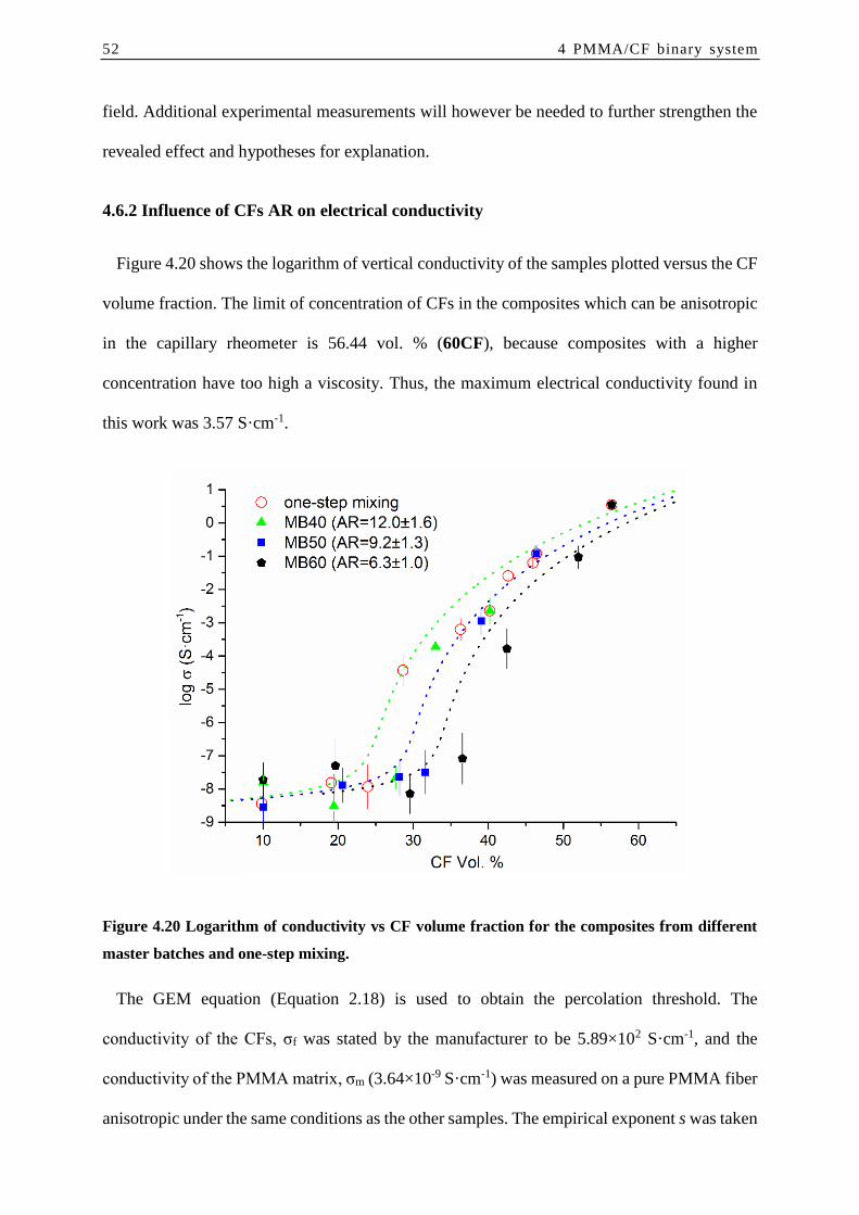
52 4 PMMA/CF binary system
field. Additional experimental measurements will however be needed to further strengthen the
revealed effect and hypotheses for explanation.
4.6.2 Influence of CFs AR on electrical conductivity
Figure 4.20 shows the logarithm of vertical conductivity of the samples plotted versus the CF
volume fraction. The limit of concentration of CFs in the composites which can be anisotropic
in the capillary rheometer is 56.44 vol. % (60CF), because composites with a higher
concentration have too high a viscosity. Thus, the maximum electrical conductivity found in
this work was 3.57 S·cm-1.
Figure 4.20 Logarithm of conductivity vs CF volume fraction for the composites from different
master batches and one-step mixing.
The GEM equation (Equation 2.18) is used to obtain the percolation threshold. The
conductivity of the CFs, σf was stated by the manufacturer to be 5.89×10² S·cm-1, and the
conductivity of the PMMA matrix, σm (3.64×10⁻⁹ S·cm-1) was measured on a pure PMMA fiber
anisotropic under the same conditions as the other samples. The empirical exponent s was taken

4 PMMA/CF binary system 53
to be 7. Due to the non-uniformed aspect ratio of the CFs from the 1st step mixing, these data
(red circles) are not further discussed.
The fitted theoretical curves in Figure 4.20 are shown with dotted lines, and the percolation
threshold φc at three different volume fraction of CFs were obtained: The percolation threshold
of composites from MB40 (green triangles) is 21.34±8.16 vol. %; of composites from MB50
(blue squares) is 26.39±4.81 vol. %; and of composites from MB60 (black pentagons) is
30.51±4.53 vol. %. From each fitted curve, the concentration with a second derivative equal to
zero (where the conductivity increases most rapidly) was also calculated as another description
of the percolation threshold: φMB40 = 25.51 vol. %, φMB50 = 30.43 vol. %, φMB60 = 34.38 vol. %,
and these values do not differ significantly from the fitted results. Composite filaments with a
higher CF AR facilitate the construction of a conductive network, and therefore reduce the
percolation threshold.
The GEM equation from McLachlan describes system with isotropic fillers. In this study, the
CFs were well oriented inside the composites and these are only small inclinations between the
CFs, which decrease the possibility for CFs to contact each other. A possible modification of
the GEM equation taking into consideration the orientation of the fillers to cover the effects
described above is left for future study.
4.6.2.1 Modification on the excluded volume theory from Balberg
In the study of Starý et al. [23], the plate-formed PMMA/CF samples were affected by
centrifugal force at 200 °C. The dispersion of CFs was not totally random, but the distribution
of orientation of the CFs was still uniform in the plane of the plate, i.e. isotropic in the range of
360°. Therefore, the value of <sin γ> (the average angle between each pair of random fibers in
the system) according to Starý was also considered as 0.64.

54 4 PMMA/CF binary system
For cylinders with L>>W in Eq. 2.3, the AR2 term in the denominator dominates, so that φc is
approximately proportional to the reciprocal of the aspect ratio (AR-1). Several reports based
on this approximation were found [23, 97-99]. In Figure 4.21 the percolation threshold φc from
literature and this study are presented with hollow symbols, which are plotted versus AR-1
(dashed horizontal axis). In the study of Yi & Choi [97] (marked with crossed inverted triangles),
extremely low percolation was reported. Because the composites were prepared below the
melting temperature, which leads to an agglomerate of CFs only on the surface of the polymer
granules. Consider following preconditions: 1. the polymer granules as perfect spheroids with
regular size; 2. the CFs exist only between them; 3. the efficiency of close packing is
approximately 0.74. In this case, the data of Yi & Choi has been divided by φc with (1 - 0.74 =
0.26) (marked with inverted triangles), in order to compare their data with the other literature.
Figure 4.21 Percolation threshold φc vs (a) dashed horizontal axis: Simplified formula from
Equation 2.4, with large AR, and regardless of <sin γ>; and (b) solid horizontal axis: complete
formula from Equation 2.4, considering <sin γ>.

4 PMMA/CF binary system 55
It is important to note that the precondition for this approximation (dashed coordinate system)
is large values of the aspect ratio (AR). If the aspect ratio is much smaller, the prediction of
percolation threshold must still follow Equation 2.4. The data calculated from the complete
formula are marked with solid symbols in the coordinate system with solid horizontal axis in
Figure 4.16. All these data fall on the same master line. The fitted result leads to K=3.4.
In a composite system with totally aligned CFs, the orientation of CFs <sin γ> is defined as
0. According to Equation 2.4, the value of φc is therefore always equal to 0.125·K, i.e. φc ≈ 42.5
vol. %, which is consistent with the totally aligned CFRP model (φc = 40 vol. %,) from
Chippendale et al. [24]. In practice, however, the CFs cannot be totally aligned. The average
<sin γ> of all the anisotropic composite filament in this study was obtained by fitting equation
2.4 (with K=3.4) to give : <sin γ> = 0.21, which is consistent with the calculated <sin γ>=0.17
of sample Nr. 60CF, and is consistent with the rough average value in Figure 4.9 . With K=3.4,
the equation from Balberg is presented in Figure 4.22, the relationship between percolation
threshold and the orientation of CFs average <sin γ> is presented.

56 4 PMMA/CF binary system
Figure 4.22 Modified equation from Balberg (Equation 2.4), with K=3.4. Fillers with different AR
in this work are presented in different color, and fillers with extreme large AR (e.g. CNTs) are
presented in dashed lines.
4.6.3 Influence of CFs orientation on electrical conductivity
The precise relationship between electrical conductivity and orientation of fillers are still
unclear. However, it is possible to compare the electrical conductivity of composites filaments
produced utilizing extrusion dies with 1-mm and 3-mm diameter, respectively, will be
compared and discussed. Since the CFs become more orientated along the extrusion direction
when using the die a smaller diameter (i.e. the D=1 mm sample contains higher oriented CFs
than that in D=3 mm sample), the relationship between electrical conductivity of the specimen
and average CFs orientation could then be investigated.
Figure 4.23 shows the logarithm of the electrical conductivity of samples plotted versus the
CF concentration. The conductivities of anisotropic composites filaments with 1-mm and 3-
0.2 0.4 0.6 0.8 1.00.0
0.00
0.05
0.10
0.15
0.20
0.25
0.30
0.35
0.40
0.45
perc
ola
tin
o t
hre
sh
old
sin gama average
AR6
AR9
AR12
AR100
AR1000
0.64

4 PMMA/CF binary system 57
mm diameter, are shown with red circles and black squares, respectively. Error bars in the
horizontal direction indicate the uncertainty in filler fraction (i.e. the difference between actual
and designed CFs volume fraction). The conductivity of pure PMMA anisotropic filament was
determined as 1.16 × 10⁻⁹ S/cm. The percolation thresholds of the composites filament were
obtained by fitting the GEM equation from McLachlan (Equation 2.18), which is presented in
Figure 4.23. The percolation thresholds φc of composites filament with 1 mm and 3 mm
diameter are: e 𝜑𝑐 (D = 1 mm) = 32.0 ± 5.9 vol. %, and 𝜑𝑐 (D = 3 mm) = 20.0 ± 2.5 vol. %. The
percolation thresholds determined by using the classical percolation theory (Equation 2.1): 𝜑𝑐(D
= 1 mm) = 31.9 vol. % and 𝜑𝑐(D = 3 mm) = 20.3 vol. %, which are consistent with the data obtained
from the GEM equation. The corresponding illustrations of the fit results utilizing Equation 2.1
are presented as insets in Figure 4.23.
During the extrusion process with the same speed of the pistol (0.08 mm/s), the composites
melt through 1-mm diameter die encountered higher shear rates ((D = 1 mm) = 92.16 s−1) and
therefore, larger shear deformations occurred for the samples with 1-mm diameter. As a
consequence, the CFs in the anisotropic filament with 1 mm diameter present a higher
orientation. Since the AR of CFs were controlled in this chapter, the average CF orientation
was the only difference between samples with 1 mm diameter and 3 mm diameter. The results
presents that a higher orientation of the CFs shift the percolation threshold to a higher CFs
volume fraction, as proved in Chapter 4.6.2. Therefore, the electrical conductivity of the
composites with 1 mm diameter is significantly lower than that of the samples with 3 mm
diameter in the region of CFs between the two percolation thresholds (20–32 vol. %).

58 4 PMMA/CF binary system
Figure 4.23 The logarithm of the electrical conductivity vs. CF volume fraction for anisotropic
filaments with 1-mm diameter and 3-mm diameter, respectively. The solid lines show the best fit
with the McLachlan equation (Equation 2.18). The two insets illustrate the linear fit using
(Equation 2.1) for the 1-mm diameter and 3-mm diameter, respectively.
Moreover, it must be noted in the Figure 4.23 that the conductivity of the specimen with 1
mm diameter (red circles) rapidly increased ca. 6 magnitudes around the percolation threshold
and then kept almost constant when the CFs volume fraction are above the percolation
threshold. However, the conductivity of the specimen (black squares) with 3 mm diameter has
only increased 3 magnitudes near the percolation threshold, but kept increasing slowly after the
percolation threshold.

4 PMMA/CF binary system 59
At CF volume fraction with approximately 50 vol. %, the specimen with 1 mm and 3 mm
diameter approached a similar value. This phenomenon can be explained by the “contact
model” [63], which is typically used for predicting conductivity CPCs with a filler volume
fraction beyond the percolation threshold (Equation 2.13).
In this chapter, the vertical conductivity is discussed, i.e. the measuring voltage was applied
along the extrusion direction of the filament and thus, the exponent cos2θ (the orientation of
CFs) increases when the tiny CFs in the CPCs become more oriented to the extrusion direction.
However, the CFs in the specimen with 1 mm diameter, were already highly anisotropic to the
extrusion direction, even at a low filler fractions (θ ≈ 0 => cos2θ ≈ 1), therefore, the cos2θ-term
from samples with 1 mm diameter almost keeps constant. Comparing to that, the CFs in the
specimen with 3 mm diameter, were firstly more isotropic at a low filler fraction, and got more
and more oriented to the extrusion direction as the concentration of CFs increases. Therefore,
the cos2θ value as well as the conductivity (which only depends on cos2θ value in Equation 2.13
in this case) of the samples with 3 mm diameter increased gradually with an increasing filler
concentration. When the CFs volume fraction in the composites reach at very high filler
fractions (beyond the percolation threshold), the CFs in both samples with 1 mm and 3 mm
diameter were highly anisotropic. Therefore, the final electrical conductivity values get similar
to each other.
It can be also noted that when the CFs volume fraction is far beyond the percolation threshold
(i.e., higher than 35%), the conductivity of the anisotropic filaments with 3 mm diameter is
lower than that with 1mm diameter. This means, an increased CFs orientation leads to a higher
electrical conductivity along the orientation direction, which is consistent with reported
literature [105-107]. Taking the morphological study into consideration, a novel approach was
proposed to explain the phenomena.

60 4 PMMA/CF binary system
4.6.3.1 A novel approach supported by the corresponding morphological study
The explanation of the different conductivities between samples with 1 mm and 3 mm
diameter lies in the volume fraction of CFs. Figure 4.24 presents a schematic interpretation of
the CFs orientation and CF volume fraction.
The first precondition of this approach is that the midpoints of CFs are fixe and the
independent CFs can only rotate around their midpoints in a 2-D system. Therefore, the CF
volume fraction depends on the midpoints of the CFs and the rotation of each CF leads to a
different CFs orientation in the CPCs. Thus, a circle is formed, considering the rotation range
of each single CF around the middle point, which is consistent with the excluded volume
concept from Balberg [65, 66]. The measuring direction of the CPCs is applied from top to
bottom of the figures, which is shown with the two-way arrows.
Based on this hypothesis, the close packing of the circles refers to the CFs volume fraction,
which just reaches the percolation threshold, i.e. the CFs just can not reach or contact each other
(Figure 4.24 (a) and (b)). In this case, there is no difference between samples with anisotropic
CFs (sample with 1 mm diameter in this case, Figure 4.24 (a)) and samples with isotropic CFs
(sample with 3 mm diameter in this case, Figure 4.24 (b)). This is the reason why the composite
filament with 1 mm diameter present a lower conductivity in the range of CFs below 15 vol. %
in Figure 4.25.
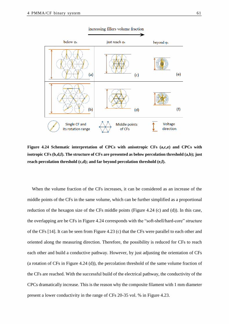
4 PMMA/CF binary system 61
Figure 4.24 Schematic interpretation of CPCs with anisotropic CFs (a,c,e) and CPCs with
isotropic CFs (b,d,f). The structure of CFs are presented as below percolation threshold (a,b); just
reach percolation threshold (c,d); and far beyond percolation threshold (e,f).
When the volume fraction of the CFs increases, it can be considered as an increase of the
middle points of the CFs in the same volume, which can be further simplified as a proportional
reduction of the hexagon size of the CFs middle points (Figure 4.24 (c) and (d)). In this case,
the overlapping are be CFs in Figure 4.24 corresponds with the “soft-shell/hard-core” structure
of the CFs [14]. It can be seen from Figure 4.23 (c) that the CFs were parallel to each other and
oriented along the measuring direction. Therefore, the possibility is reduced for CFs to reach
each other and build a conductive pathway. However, by just adjusting the orientation of CFs
(a rotation of CFs in Figure 4.24 (d)), the percolation threshold of the same volume fraction of
the CFs are reached. With the successful build of the electrical pathway, the conductivity of the
CPCs dramatically increase. This is the reason why the composite filament with 1 mm diameter
present a lower conductivity in the range of CFs 20-35 vol. % in Figure 4.23.

62 4 PMMA/CF binary system
When the CF volume filler fractions increases beyond the percolation thresholds (Figure 4.24
(e) and (f)), i.e. conductive network are formed in both CPCs, and filament with 1 mm and 3
mm diameter turn to be both conductive. However, the difference between two kinds of
conductive pathways must be noted: (1) along one single CF; (2) transfer between the contact
points between two connected CFs. It can be logical that the first pathway is more efficient with
a higher conductivity, which appears more in the system with oriented CFs, as presented in
Figure 4.24 (e). Therefore, the CPCs with oriented CFs along the measuring direction presents
a higher conductivity than that with isotropic CFs. This is the reason why the composite
filament with 1 mm diameter present a higher conductivity in the range of CFs higher than 35
vol. % in Figure 4.23.
Figure 4.25 (g) presents a general morphological picture of the PMMA/CF CPC filament,
where a single carbon fiber and the extrusion direction were shown. Figure 4.25 (a)-(f) present
the fiber orientation in anisotropic composite filament with 10 vol. % (Figure 4.25, (a)(b)), 30
vol. % (Figure 4.25, (c)(d)) and 50 vol. % CFs (Figure 4.25, (e)(f)) respectively. The upper row
of figures (Figure 4.25, (a)(c)(e)) refers to the filament with 1 mm diameter, containing more
oriented CFs; the lower (Figure 4.25, (b)(d)(f)) refers to the filament with 3 mm diameter,
containing less oriented CFs. It can be noted that the CFs in the filament with 3 mm diameter
are more isotropic than that in the 1 mm diameter filament. Moreover, it can be seen that the
orientation of the CFs increases, as the filler fraction increases. This is the certificate of the
novel approach in Figure 4.24.

4 PMMA/CF binary system 63
Figure 4.25 Morphological study on the orientation of inner CFs with 1-mm diameter (g,a,c,e) and
with 3-mm diameter (b,d,f). (a)(b) show filament with 10 vo.% CFs, which is below percolation
threshold; (c)(d) show filament with 30 vo.% CFs, which just reach percolation threshold; (e)(f)
show filament with 50 vo.% CFs, which far beyond percolation threshold.
4.7 Conclusion
In Chapter 4, PMMA/CF anisotropic filament are presented. The CPCs were produced under
high concentration (Chapter 4.2). Different lengths of CFs (with aspect ratios 6.3, 9.2, and 12.0,
respectively) were obtained with a two-step melt mixing process (Chapter 4.4). Due to the
extrusion process, highly anisotropic CFs were obtained in the composites, presenting a “fibers
in fiber” structure (Chapter 4.3). Moreover, due to the shear gradient across the channel section,
the CFs orientation were decreased from the outer part of the composite to the center (Chapter
4.5)

64 4 PMMA/CF binary system
In Chapter 4.6.1, the vertical and horizontal electrical conductivity of the anisotropic
anisotropic PMMA/CF composite with 3 mm diameter were discussed. The “peeling-off” and
“polishing” methods were developed, in order to reveal different conductivity in the radial
direction of the composites filament.
In Chapter 4.6.2, the vertical electrical conductivity of PMMA/CF filaments with 1 mm
diameter were revealed. The conductivity of composite filaments at room temperature was
compared with the McLachlan GEM equation and Balberg excluded volume theory. An
increase the filler aspect ratio led to a decrease in the percolation threshold. Taking into
consideration the filler orientation, the slope K=3.4 in excluded volume theory was estimated
for the first time.
In Chapter 4.6.3, the conductivity of PMMA/CF filaments (with controlled aspect ratio of
CFs) with 1-mm and 3-mm diameter were compared. The results show that a higher orientation
of the CFs can shift the percolation threshold to a higher volume fraction. However, when the
CFs volume fraction beyond the percolation threshold, a higher orientation of the CFs along the
measuring direction leads to a higher conductivity of the CPCs. A novel explanation based on
the morphological study was proposed to explain the phenomenon.

5 PMMA/CB/CF ternary system

66 6 PMMA/CB/CF ternary system
5.1 Introduction
Besides carbon fibers (CFs), carbon black (CB) is also the most commonly used conductive
fillers, which can be incorporated into a polymer matrix for facilitating the formation of a CPCs.
In this chapter, the electrical conductivity of anisotropic composites filament consisting of
PMMA containing both aligned carbon fibers (CF) and carbon black (CB) will be presented. A
broad range of composite compositions (up to 50 vol. % CF and 20 vol. % CB) has been studied.
The CB (XE2) used in this chapter is highly structured and the primary particles are fused to
small aggregates which in turn form agglomerates [14], resulting in a significantly reduced
percolation threshold. As discussed in Chapter 4, the PMMA/aligned CFs composites filament
presents a higher percolation threshold than those with isotropic CFs. Therefore, the study on
the conductivity of PMMA/aligned CFs/CB has arisen the interests.
Literature exist reporting a synergistic effects of CPCs containing both CFs and CB [108-
112]. In a system with isotropic CFs and CB particles, clusters of CB may form short
“conductive pathways” between the CFs. Therefore, the conductivity of composites containing
both fillers can be enhanced, as compared to those with only CFs or CB at the same
concentration of fillers.
Figure 5.1 Schematic of the conductive pathway formed by CB and CFs in the CPCs. (a) CPCs
with isotropic CFs, conductive pathway are contributed also by CFs themselves; (b) CPCs with
highly orientated CFs, the contacts between CFs are reduced. With the addition of CB particles,
a fence-like structure can be formed; (c) cross section view of composite filament with fence-like
structure.

5 PMMA/CB/CF ternary system 67
However, in a CPC system with isotropic fillers (Figure 5.1(a)), the contribution of
conductive pathways formed between CFs themselves to the conductive networks must also be
considered [108-112]. In order to evaluate the real synergic effect between CFs and CB, the
effect of the CF-pathways in a PMMA/CB/CF system should be minimized. Therefore, the
extrusion process is applied, in order to induce a maximum alignment of the CFs in the CPCs
and consequently, to reduce the contacts between the CFs. With the addition of CB particles,
“conductive pathways” can also be formed between the parallel CFs, such that fence-like
structure is formed. (A side view and a cross section view of an idealized fence-like geometry
is shown in Figure 5.1 (b) and Figure 5.1 (c), respectively). Thus, the real synergistic effect
between CB and CFs in an anisotropic composite filament can be then revealed.
Synergistic effects were also reported between CB and carbon nanotubes (CNT) in ternary
composites [113-115]. CNT and CF are both suitable conductive 1-D fillers. In this chapter,
CFs were chosen at first due to their (1) improved melt mixing dispersion (2) more distinct
cylindrical shape, (3) larger size, which simplifies microscopy analysis and (4) higher
percolation threshold, which enabled a more genuine validation of our analytical conductivity
model.
Several theories [116, 117] have been suggested to describe the conductivity of binary
composites, but few models consider the conductivity of ternary composites with two
conductive fillers. Sun et al. [81] have proposed a percolation threshold model based on the
assumption that the excluded volume of the two fillers can be added together linearly. The
percolation threshold of a conductive composite with two fillers can then be predicted as
Equation 2.21. Therefore, a conductivity contour plot versus φCFs and φCB was presented in this
chapter, such that the linear Equation 2.21 could be evaluated.
Since the experimental conductivity measurements did not fully support Equation 2.21, an
improved original equation was proposed in this work for predicting the electrical percolation
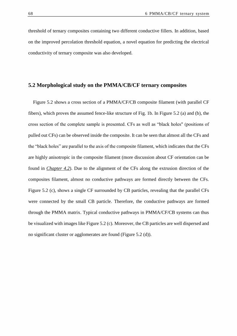
68 6 PMMA/CB/CF ternary system
threshold of ternary composites containing two different conductive fillers. In addition, based
on the improved percolation threshold equation, a novel equation for predicting the electrical
conductivity of ternary composite was also developed.
5.2 Morphological study on the PMMA/CB/CF ternary composites
Figure 5.2 shows a cross section of a PMMA/CF/CB composite filament (with parallel CF
fibers), which proves the assumed fence-like structure of Fig. 1b. In Figure 5.2 (a) and (b), the
cross section of the complete sample is presented. CFs as well as “black holes" (positions of
pulled out CFs) can be observed inside the composite. It can be seen that almost all the CFs and
the “black holes” are parallel to the axis of the composite filament, which indicates that the CFs
are highly anisotropic in the composite filament (more discussion about CF orientation can be
found in Chapter 4.2). Due to the alignment of the CFs along the extrusion direction of the
composites filament, almost no conductive pathways are formed directly between the CFs.
Figure 5.2 (c), shows a single CF surrounded by CB particles, revealing that the parallel CFs
were connected by the small CB particle. Therefore, the conductive pathways are formed
through the PMMA matrix. Typical conductive pathways in PMMA/CF/CB systems can thus
be visualized with images like Figure 5.2 (c). Moreover, the CB particles are well dispersed and
no significant cluster or agglomerates are found (Figure 5.2 (d)).

5 PMMA/CB/CF ternary system 69
Figure 5.2 SEM micrographs of cross sections of composite filament with different magnification,
sample: 2CB3CF.
5.3 Conductivity of the composite filament
5.3.1 Percolation threshold of binary PMMA/CF and PMMA/CB samples
For PMMA/CB and PMMA/CF binary composites filament, the electrical conductivity, as a
function of filler fraction, is presented in Figure 5.3. The X- and Y-axis present the CB and CF
volume fractions in the composites filament, respectively. Until now, several models have been
proposed to describe percolation phenomena at critical levels of conductive fillers and to predict
the electrical conductivity behavior of CPCs. The most classical percolation theory equation is
Equation 2.1 [48-49]. For composites with filler concentrations φ>φc, the experimental results
(a) (b)
(c) (d)

70 6 PMMA/CB/CF ternary system
are fitted by plotting log σ against log (φ-φc) and regulating φc until the best linear fit is obtained.
Thus, the estimated percolation thresholds for the anisotropic PMMA matrix composite
filament become: φc, CB =3.9 vol. %, and φc, CF =31.8 vol. % (Figure 5.3), which is consistent
with the percolation threshold of PMMA/CF 30.43 vol. % as reported in Chapter 4.6.2. A strong
alignment of the anisotropic CFs was induced by the extrusion process, and consequently, the
percolation threshold of the PMMA/CFs composite filament becomes much higher than of the
reported PMMA/CFs binary composites filament with isotropic CFs [108-112].
Figure 5.3 Conductivity of PMMA/CF and PMMA/CB composites vs. filler volume fraction in
three-dimensional coordinates. Standard deviations, based on 10 measurements/data points, are
shown with error bars. The two insets illustrate the linear fit of the t-value for PMMA/CF (red
square) and PMMA/CB (blue spheroids), respectively.
5.3.2 Contour plot of conductivity on PMMA/CB/CF ternary composite
A conductivity contour plot diagram based on the experimental data (binary composites
and ternary composites) is presented in Figure 5.4, where the X-axis and Y-axis correspond to

5 PMMA/CB/CF ternary system 71
CB volume fraction and CF volume fraction, respectively. The black squares on the contour
plot show the composition of CF and CB from actual tested samples. The 10-logarithm of the
electrical conductivity of CPCs is presented in colors while iso-contour lines equating 1
magnitude are drawn in black. The composite conductivity obviously increases steeply with
growing filler concentration.
Figure 5.4 Logarithm value of conductivity of composite filament as a function of filler volume
fraction of CFs and CB in a contour plot diagram presented in this work.
The percolation concentrations of CB and CF are marked on the X-axis (3.9, 0) and Y-axis
(0, 31.8), respectively. The white dashed diagonal line a (Y=-8.17X+31.8), which connect the
two percolation points, correspond to Equation 2.21 with K=1, showing the predicted
percolation threshold of the ternary composites. The percolation threshold should follow this
line if the excluded particle volumes are linearly additive, i.e. if Equation 2.21 is valid.
The dramatic changes in electrical conductivity must be considered, when the volume fraction
of fillers is near the percolation concentration, which can result in a large standard deviation for
72 6 PMMA/CB/CF ternary system
the experimental measurements (See Figure 5.3). Therefore, two additional parallel lines (line
b and c) were also added on the contour plot, with fillers volume fraction are above the
percolation threshold. Line c was created by passing the maximum investigated CF volume
fraction (0, 50), with the same slope as line a. The intermediate value of y-intercepts from line
a and line c, was applied as the y-intercept of line b. These lines correspond to K=1.28 and
K=1.56, i.e. filler fractions 1.28 respective 1.56 times larger than the presented percolation
threshold filler fractions.
Conductivities of composite filament with CF/CB compositions following the three diagonal
lines were investigated and presented in Figure 5.5. For all three diagonal lines (on X-Y plane),
the conductivities (Z value) at the ends of the line were higher than in the middle, indicating a
negative collective effect between CB and aligned CFs. This result is in agreement with the
right-pointed protrusion (positive curvature) of contour lines in Figure 5.4, which is in contrast
to the slight “synergetic effect” [108-112] previously observed. However, small protrusions to
the left of the contour lines can be still observed for CF filler fractions below 10 vol. %,
indicating local synergetic effects similar to those previously reported [108-112].
The conductivity contour-lines of the composites filament are clearly concave and materials
showing synergetic effects must by definition also show non-linear behavior. In order to
describe such materials, the linear assumption of Equation 2.21 is thus clearly not valid,
although the equation still can be used for determining synergy. Therefore, an extended and
more general equation is required for predicting the conductivities of CPCs containing two (or
more) fillers.

5 PMMA/CB/CF ternary system 73
Figure 5.5 Logarithm value of conductivity of composites with composition of CFs/CB on the three
diagonal lines (from Figure 5.4) vs. filler volume fraction of aligned CFs and CB in this work.
As a complement to the measurements, the literature on conducting polymer composites with
isotropic CF and CB in polymer matrix (thermosetting based shape-memory polymer [29],
acrylonitrile butadiene styrene [108] and polypropylene [109-111]) have been reanalyzed and a
conductivity contour plot of the results is presented in Figure 5.6. The literature data present
higher composite conductivities than the data from the anisotropic composite filament in this
work (Figure 5.3), probably mainly because the axial CF-orientations in this work obstruct the
construction of conductive networks and thus reduce the composite conductivities. It should
thus also be noted that the polymer matrix in the literature review is other polymer matrix
instead of PMMA in this study.

74 6 PMMA/CB/CF ternary system
Figure 5.6 logarithm value of conductivity of composite filament vs. filler volume fraction of CFs
and CB in a contour plot diagram on the basis of literature reanalysis.
5.4 Novel equations for electrical behavior of ternary composite
If Equation 2.21 would hold, the iso-curve between φc,CB and φc,CF in Figure 5.4 would be a
straight line. Since the measured electrical conductivities showed distinctly curved iso-curves,
a new equation was required for describing the percolation behavior of CPC’s containing two
kinds of fillers more accurately. This conclusion was also strengthened by literature data [108-
110], showing synergetic (i.e. non-linear) effects by combining certain kinds of conductive
fillers. In order to simplify the mathematical expressions in Equation 2.21, the relative filler
fractions α and β were introduced, which are defined as the ratios between present volume
fraction φ and percolation threshold φC, for CFs and CB, respectively:
CFcCF ,/ (5.1)

5 PMMA/CB/CF ternary system 75
CBcCB ,/ (5.2)
Equation 2.21 could thus be reformulated as:
K (5.3)
A corresponding improved non-linear equation should be able to describe both linear,
concave and convex curves and give correct values at α =0 or β =0. The least complicated
function fulfilling those criteria is probably:
𝑍 = (𝛼𝑁 + 𝛽𝑁)𝑁 (5.4)
where the physical meaning of Z is the same as K in Equation 2.21 and Equation 5.3, i.e. when
Z=1, the percolation threshold just reached. κ is an adjustable interaction parameter. If N =1 the
equation becomes linear, if N <1 the two fillers are synergetic and if N >1 the fillers are anti-
synergetic. Equation 5.4 can thus be used as an improved alternative to Equation 2.21 for
describing the percolation threshold of CPCs containing two fillers. The ‘synergy’ can also be
defined as: when the curvature parameter N becomes smaller than 1 when the experimental data
is fitted to Equation 5.4.
However, the property of main interest is often the composite conductivity rather than the
percolation threshold. Therefore, an equation for predicting the conductivity of three-
component composites was also developed. The conductivity of a composite containing only
one filler can often be accurately described, as function of filler fraction φ, with the McLachlan
Equation 2.18 [67, 68]. The hypothesis for the novel equation was that a linear combination of
the conductivities of two binary composites, each with one single type of filler, could be used
to describe the conductivity of a ternary composite, containing both types of fillers. This
hypothesis correspond to coupling the binary composites in parallel. According to this
hypothesis, the new equation (assuming CB and CF fillers) could be written as:

76 6 PMMA/CB/CF ternary system
CBCBcCFCFcCBCFtot ZZ ,, ,1min,1min),(
(5.5)
The single-filler percolation thresholds φc,CF and φc,CB as well as the φ-dependent single-
filler conductivities σ(φCF)CF and σ(φCB)CB are determined with Equation 2.18. As a safety
routine, a restriction was added such that the functions could not exceed the values of their
corresponding filler conductivities.
The prediction capability of Equation 5.5 was evaluated using the experimental data
presented in Figures 5.3-5.5. As a first step, the single filler conductivities of PMMA/CB and
(un-axial) PMMA/CF composites filament were fitted with the McLachan equation (Equation
2.18), resulting in two log(σ) versus φ curves. The estimated filler conductivities were σCB
=1.34*102 S/cm for CB and σCF=4.06 S/cm for CF. The fitted percolation thresholds with
McLachan equation were φc,CF =33.5 vol. %. and φc,CB =3.9 vol. %, which are consistent with
the value obtained from Eq. 3: φc, CF =31.8 vol. % and φc, CB =3.9 vol. %. The result, as presented
in Figure 5.7, shows a good agreement between the experimental conductivities and the best fit
of Equation 2.18.

5 PMMA/CB/CF ternary system 77
Figure 5.7 Conductivity of composite filament vs. filler volume fraction of aligned CFs and CB,
fitting with McLachlan equation to determine the electrical conductivity of fillers in the
anisotropic fiber consisting of ternary composites.
Equation 5.5, as implemented in the Matlab(R) software, was then used for creating a two-
dimensional conductivity contour plot. Equation 2.18 (with parameters as in Fig. 5.7: σCF, σCB,
φc,CF, φc,CB), and Equation 5.4 (with N = 1.47) were used as input. The resulting model waterfall
plot (Figure 5.8) and contour plot (Figure 5.9) show a trend which fits the corresponding the
experimental contour plot (Figure 5.4) well.

78 6 PMMA/CB/CF ternary system
Figure 5.8 Logarithm value of conductivity of composite filament vs. filler volume fraction of CFs
and CB in a waterfall plot diagram, as generated with equation 5.8.
Figure 5.9 Logarithm value of conductivity of composite filament vs. filler volume fraction of CFs
and CB in a contour plot diagram, as generated with equation 5.8.

5 PMMA/CB/CF ternary system 79
Finally, Equation 5.5, with settings as above, was compared to the experimental
conductivity data along the three lines of Figure 5.6. The result was presented in Figure 5.10.
Since the experimental non-linear trend was approximately in agreement with Equation 5.5, the
new equations are clearly more accurate than previously existing models for describing the
electrical conductivity and the percolation threshold for composites containing two different
conductive fillers.
Figure 5.10 Logarithm value of conductivity of composite filament vs. filler volume fraction of CB
in a 2-D coordinates system. Filled symbols represent experimental data while solid lines represent
the simulation curves with predicted data from Equation 5.8, where line a-c are from Figure 5.4.
5.5 Conclusion
In this study, anisotropic PMMA/CB/CF ternary composites filament, with a broad range of
composites compositions (up to 50 vol. % CF and 20 vol. % CB) were studied. SEM
micrographs exposed a “fence-like” morphological structure between the CB and the CF.
80 6 PMMA/CB/CF ternary system
Electrical conductivity measurements were used to determine the electrical percolation
thresholds of binary PMMA/CF and PMMA/CB composites filament and to reveal the relation
between filler fraction and the ternary composite filament conductivity for PMMA/CB/CF.
Conductivity contour plots, showing conductivity as a function of filler fraction, were presented
for PMMA/CF/CB composites filament for the first time; one extensive plot based on data from
this study and one based on already existing literature data. Distinctly curved iso-lines were
observed. Synergetic effects between CFs and CB were found in the regions below 10 vol. %
CF, observed as left-pointed protrusions of the contour-lines. Moreover, based on a model for
predicting the percolation threshold of ternary composites, a novel equation for predicting the
electrical volume conductivity of ternary composites was proposed, showing results close to
corresponding experimental data. Since the study in this chapter comprises highly systematic
measurements of electric conductivity for PMMA/CB/CF composites as well as the novel and
significantly improved effective-media equations for conductive ternary composites, it provides
a general guidance for the design and analysis of CPC.

6 PMMA/CB/CNTs ternary system

82 6 PMMA/CB/CNTs ternary system
6.1 Introduction
Conductive polymer composites (CPCs) are promising materials for many electrical
applications due to their high conductivity, low weight and simple processing [70-73]. Carbon
nanotubes (CNTs) and carbon black (CB) are two of the most commonly used conductive fillers
in CPCs [74-79]. Several studies on ternary CPCs comprising CNTs and CB have recently been
reported, indicating that the electrical properties of ternary composites comprising CB and
CNTs can potentially be superior to corresponding binary CF- or CB-composites [80-88]. The
conductivity of binary CPCs can be modeled, as a function of filler fraction, with several
existing analytical models from the literature [57-64]. McLachlan's general effective medium
(GEM) equation [67, 68] (Equation 2.18) is probably the most reliable equation that can model
the composite conductivity both below and above the electrical percolation threshold.
The conductivities of ternary composites can also be modeled with analytical expressions,
but the number of existing models is far more limited [81]. Sun et al [81] suggested that the
percolation threshold of a ternary composite can be approximated by a straight line between the
percolation thresholds of the two different fillers. If φCNT and φCB are the (volume or weight)
fractions of CNTs and CB while φc,CNT and φc,CB are the percolation thresholds of CNT and CB
in binary composites (Equation 2.21), then Suns expression becomes:
1,,
CNTc
CNT
CNTc
CNT
(6.1)
The experimentally observed percolation threshold for ternary carbon fiber (CF) / CB
composites was however rather a convex curve than a straight line between φc,CNT and φc,CB.
Therefore an improved equation was suggested in Chapter 5.4.
Equation 5.4, which describes the curvature of the percolation threshold for ternary
composites, was used to derive a corresponding conductivity equation. The conductivities for
the binary composites (denoted σCB for the CB and σCNT for the CNT) can be calculated with

6 PMMA/CB/CNTs ternary system 83
Equation 2.18 and the expression for the ternary composites, which was successfully applied
on CF/CB composites (Equation 5.5).
A “synergistic effect” is often reported for ternary composites with CB and CNTs [72, 74-
88]. One possible explanation for an eventual “synergistic effect” is that electrical pathways
could potentially form more easily in ternary CNT/CB composites than in binary CNT- or CB
composites since the small, spherical CB fillers bridges the long CNT-fillers and thus improves
the contacts in the resulting electrical network [79, 83], [82, 85]. However, several definitions
of “synergy” exist, and the choice of definition will strongly influence the conclusion on
whether a ternary composite is subject to “synergy” or not. The current classifications of
“synergy” are:
1st synergy: When a “small amount” of a second filler “dramatically” increases the
conductivity of the CPC.
2nd synergy: When the conductivity of the ternary CPC is higher than the conductivity
of either of the two binary CPCs, while keeping the total filler fraction constant.
3rd synergy: When the experimental percolation threshold of the ternary CPC is lower
than the predicted straight line between the percolation thresholds of the two fillers
(Eq.2).
4th synergy: When the curvature parameter N becomes smaller than 1 when the
experimental data is fitted to Equation 5.5.
The 1st synergy criterion has been fulfilled for a few ternary CNT/CB composites [74, 75].
The 2nd synergy criteria and a suggested optimal ratio between CNTs and CB has been
discussed in several studies [77, 80, 82-86, 88] and also the 3rd synergic effect between CFs and
CB have often been mentioned [77, 78, 82-88]. The definition of the 4th synergy, which is
closely related to the definition of the 3rd synergy, was presented in Chapter 5. It should be

84 6 PMMA/CB/CNTs ternary system
noted that the previously published conductivity data for ternary CNT/CB composites is overall
rather limited.
The true “synergistic effect” between the two fillers of a ternary composite can only be
revealed with a reliable conductivity contour plot covering a broad volume fraction range of
each filler. Such a contour plot has previously been presented for ternary carbon fiber (CF)/CB
composites, but never for CNT/CB mixtures. The aim of this study is to make and analyze such
a conductivity contour plot for ternary CNT/CB composites.
In order to minimize the interaction between the CNTs themselves and thus highlight the
interaction between the CNTs and the CB, the ternary CPCs specimen of this study were
anisotropic from a capillary rheometer. The aim was to induce an orientation of the CNTs and
reduce the contacts between the CNTs. The resulting composites become anisotropic, while the
existing literature mainly discusses CPCs with isotropic orientation of CNTs [75-80, 82-84, 86-
88].
6.2 Morphology of the ternary composite filament
Figure 6.1 shows (a) the cross section (b) the middle section of a ternary composite filament
with 5.44 vol. % CNTs and 6 vol. % CB. In Figure 6.1(a), the CNTs (brighter dots) were found
to be perpendicular to the flat page (or the plane of the paper). Because the diameter of the
CNTs were similar to the diameter of the primary CB particle, it is difficult distinguish the
CNTs and CB. In Figure 6.1(b), the CNTs were oriented along the extrusion direction, and the
CB aggregates were found to be located between them. This “grape-like” structure is the
theoretical basis of the reported “synergy” between CB and CNTs as reported before [82, 86].

6 PMMA/CB/CNTs ternary system 85
Figure 6.1 Morphology of the anisotropic ternary CPCs filament with 5.44 vol. % CNTs and 6
vol. % CB: (a) the cross section of the specimen; (b) the middle section of the specimen.
6.3 Conductivity of the binary PMMA/CNTs and PMMA/CB composite
Figure 6.2 shows the logarithm of the conductivity plotted versus the CB (black squares) and
CNT (red circles) volume fraction, respectively. Each data point represents the average of 10
measurements, with standard deviations shown with vertical error bars. Horizontal error bars
indicate the uncertainty in filler fraction. The data was fitted with the McLachlan equation,
(Equation 6.1) and the percolation thresholds were determined to φc,CB=3.9 vol.%, φc,CNTs=5.0
vol.%. The reliability of the McLachlan percolation thresholds was confirmed by comparing
the results with another classical percolation theory equation (Equation 2.1). For composites
with filler concentrations φ>φc, the experimental results were fitted by plotting log σ versus φ,
as presented in the insets of Figure 6.2, also resulting in φc,CB=3.9 vol.%, φc,CNTs=5.0 vol.%.

86 6 PMMA/CB/CNTs ternary system
Figure 6.2 The logarithm of the conductivity vs. filler volume fraction of CNTs and CB,
respectively. The solid lines show the best fit with the GEM equation (Equation 2.21). The two
illustrate the linear fit using (Equation 2.1).
The conductivity curves for CB and CNT were surprisingly similar, considering that the
electrical percolation threshold typically decreases when the aspect ratio (i.e. length/width) of
the particles increases [23]. A lower φc would thus have been expected for the strongly
elongated CNTs than for the almost spherical CB. The explanations for the non-intuitive
experimental results are that (1) CB aggregates in a structured way that increases the effective
aspect ratio and conductivity [90] and (2) the shear-induced fiber orientations increases the
percolation threshold for the oriented CNT composites as compared to more isotropic CNT-
composites. Kim has reported a similar electrical behavior for binary CPCs containing CB and
oriented CNTs [73]. Therefore, the “synergy” between CB and oriented CNTs could be

6 PMMA/CB/CNTs ternary system 87
different in this study than that between CB and isotropic CNTs as reported before [75-80, 82-
84, 86-88]. Schematic electrical networks in anisotropic composites, comprising either CNT or
CB, are presented in Figure 6.3.
Figure 6.3 Schematic structure of electrical pathway formed by (a) CNTs and (b) CB particles in
a binary CPC system.
6.4 Experimental contour plot of conductivity on ternary composite
A logarithmic contour plot based on the experimental conductivity data is presented in Figure
6.4, where the X- and Y-axis correspond to CB- and CNT-volume fraction, respectively. The
filler fraction range was maximized with respect to the capability of the capillary rheometer. At
higher filler fractions the viscosity grew so high that the composites could not be extruded out
of the die. The black squares on the contour plot are the actual tested samples while the black
iso-contour lines correspond to 1 magnitude conductivity differences. The conductivity
increases steeply with growing filler concentration, especially near the percolation threshold
curve (red solid line). The results of Figure 6.4 will be systematically analyzed using the four
definitions of synergy.

88 6 PMMA/CB/CNTs ternary system
Figure 6.4 Logarithm value of conductivity of composite filament vs. filler volume fraction of
CNTs and CB in a contour plot diagram, with definition on traditional 1st-3rd synergy.
The 1st synergy, which is fulfilled when a small addition of a second filler do not radically
increase the conductivity, was not clearly observed for any of the experimental data points.
Anyway, according to the shape of the contour-lines, two regions with potential 1st synergy
could eventually be present at high filler contents along the X- and Y-axis, as marked with
green solid lines. This possibility is however not confirmed experimentally and the eventual
synergetic conductivity increase must anyhow be weak since the material is already percolated.
It could also be argued that some ternary composites just above the percolation could fulfill the
1st synergy criterium, but since a similar conductivity increase would occur also for
corresponding binary composites, this argument is rather weak. Overall, the 1st synergy
criterion is undesirably inexact and should generally be avoided when evaluating synergy of
ternary composites.

6 PMMA/CB/CNTs ternary system 89
The 2nd synergy definition is fulfilled when the conductivity of the ternary CPCs is higher
than the conductivity of either binary CPC, while keeping the total filler fraction m=(φCNT + φCB)
constant. This criterion is satisfied for any point C (along the magenta-colored line y=m-x) with
higher conductivity that the conductivities of points A=(0,m) and B=(m,0). From the contour
lines of Figure 6.4, it can be observed that the second synergy criterion is probably fulfilled at
high filler fractions, but at low fillers contents the composites are rather anti synergetic.
The 3rd synergy definition is fulfilled if the percolation threshold contour curve (red solid
curve in the inset of Figure 6.4) is primarily situated below the line of Equation 6.1, which is
the dashed, red, diagonal, straight line (Y=-1.28X+5) going between the CNT percolation
threshold (0, 5) and the CB percolation threshold (3.9, 0). This synergy criterion is obviously
not fulfilled for our ternary CNT/CB composites, which is in agreement with several previous
studies [77, 83, 84, 88].
The 4th synergy, which is a more precise extension of the third definition, confirms that the
composite is dominantly anti-synergetic, because fitting with Equation 5.4 gives a curvature N
=1.3, which is clearly higher than unity. Figure 6.5 visualizes the conductivities calculated with
Equation 5.5 and the inset figure shows Equation 5.5 (solid lines) together with experimental
data (symbols) along four diagonal lines parallel to Equation 6.1 (dashed lines in Figure 6.5).
The modeling results are in reasonable agreement with the experimental measurements. It can
be noted that the curvature of the CNT/CB composites was qualitatively similar to the curvature
of ternary CF/CB composites.

90 6 PMMA/CB/CNTs ternary system
Figure 6.5. Logarithm of the composite conductivity versus volume filler fraction of CNTs and CB
in a contour plot, as generated with Equation 5.5. The inset show experimental- and modeled data
along the four dotted lines.
6.5 Reanalysis of the literature
As a complement to our measurements and modeling results, the literature on ternary
composites with CNTs and CB in a polymer matrix (HDPE [91], TPU [92], epoxy resin[93],
UHMWPE [94], PVDF [75], PA6/ABS blend [78], PLA [79], PBT [80], Silicone Rubber [82],
TPE [83], PA12 [84], PP [85], PP-g-MA [86], PC [88]) was reanalyzed. Among these studies,
Chen et al. [78], Wu et al. [79], Dorigato et al. [80], Wen et al. [85] and Zhang et al. [86]
reported synergetic effects according to the 2nd or 3rd definition. The results are summarized in
Figure 6.6, showing the filler fractions where synergy has been reported for ternary CB/CNT
composites.

6 PMMA/CB/CNTs ternary system 91
Figure 6.6 The composition between CNTs and CB reported in the literature, with different results
on ‘synergy’.
In contrast to the results of this paper, several studies from the literature have reported synergy
effects for ternary CNTs/CB composites. One possible reason for this discrepancy could be that
this study concerns oriented CNTs while most other studies have isotropic orientation of the
fillers. The choice of matrix material could also influence, due to eventual segregation effects.
Another explanation could simply be the difficulty of measuring and interpreting conductivity
results. For example, since the standard deviation is typically very high when measuring the
conductivity of composites close to the percolation threshold, it is easy to draw erroneous
conclusions based on statistical variations and random errors. In several of the mentioned
studies, the number of replicates is low or unknown, which accentuates the problem, because
the impact of single outliers increases. Several of the reported synergies are also based on
extrapolated data rather than comparisons between actual samples. Overall, even if synergies
between CNTs and CB could potentially exist, the hitherto presented pieces of evidence of

92 6 PMMA/CB/CNTs ternary system
synergetic effects are surprisingly limited and could in worst case simply be the effect of
statistical variations.
As for the 1st synergy, can be described as the increase of the conductivity from the green
dashed line along either the X-axis (PMMA/CB binary system) or the Y-axis (PMMA/CNTs
binary system) to the green solid line. Figure 6.7 presents a schematic definition on the 1st
synergy, where some CNTs were added into the PMMA/CB binary system. Although this
synergy is found in our study accordingly, 1st synergy is believed to be an improper definition
due to the unfixed variable filler volume fraction.
Figure 6.7 Schematic definition on the 1st synergy, corresponds to Equation 2.23.
Additionally, the limit of 2nd synergy is only a comparison between the conductivity of
ternary CPCs with the binary CPCs, always expanded proportionally (Figure 6.8). Dorigato et
al. [80] presented the 2nd synergy with different m values as described in Figure 6.8. However,
the total filler fraction m were kept always below the percolation threshold of binary CPCs with
CB, which leads to a higher conductivity of ternary CPCs than the binary CPCs with CB below
percolation threshold. Wu et al. [79] has reported the conductivity of pre-foamed and post-
foamed CPCs (without any deviation on the conductivity), the 2nd synergy was found to exist
only after foaming (Anti synergy was reported before foaming). Nevertheless, Wen et al. [85]
reported a 2nd synergy between CNTs and CB after CPCs prepared by stretching extrusion only,
and an anti-synergy was presented without stretching.

6 PMMA/CB/CNTs ternary system 93
Figure 6.8 Schematic definition on the 2nd synergy, corresponds to Eq. 2.24
Moreover, the 3rd synergy focus on the percolation region, where a large standard deviation
for the experimental measurements exist. Chen et al. [78] has produced binary CPCs with max.
4 wt. % CB, and chose the point 4 wt. % as the percolation threshold. This value is used in
Equation 6.5 to calculate the ternary percolation threshold as 0.97 wt. %, slightly higher than
0.8wt. %, as a prove of 3rd synergy. Besides, the reproducibility of the specimen could be also
questioned, due to no error bars on the presented conductivities. Zhang et al. [86] reported 10
volume fractions of the total filler content above the percolation threshold with CNT wt. %/CB
wt. %=1, and only 9 volume fractions were used to obtain the extremely low experimental
ternary percolation threshold as 0.21wt. % using Equation 6.5. Comparing with the calculated
ternary percolation threshold 3.0 wt. % using Equation 2.21, the most obvious 3rd synergy is
presented.
Therefore, to our best of knowledge, no convincing results were found according to the
common defined three “synergy”. Since the ternary CPCs has one more dimension (σ, φ1, φ2)
than the traditional binary CPCs (σ, φ), a new definition on the electrical interaction between
CNTs and CB is thus required.
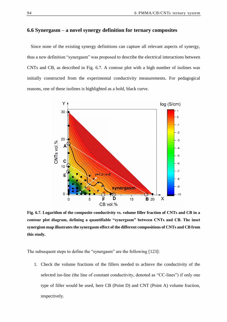
94 6 PMMA/CB/CNTs ternary system
6.6 Synergasm – a novel synergy definition for ternary composites
Since none of the existing synergy definitions can capture all relevant aspects of synergy,
thus a new definition “synergasm” was proposed to describe the electrical interactions between
CNTs and CB, as described in Fig. 6.7. A contour plot with a high number of isolines was
initially constructed from the experimental conductivity measurements. For pedagogical
reasons, one of these isolines is highlighted as a bold, black curve.
Fig. 6.7. Logarithm of the composite conductivity vs. volume filler fraction of CNTs and CB in a
contour plot diagram, defining a quantifiable “synergasm” between CNTs and CB. The inset
synergism map illustrates the synergasm effect of the different compositions of CNTs and CB from
this study.
The subsequent steps to define the “synergasm” are the following [123]:
1. Check the volume fractions of the fillers needed to achieve the conductivity of the
selected iso-line (the line of constant conductivity, denoted as “CC-lines”) if only one
type of filler would be used, here CB (Point D) and CNT (Point A) volume fraction,
respectively.

6 PMMA/CB/CNTs ternary system 95
2. The filler with the lower required volume fraction to achieve the selected conductivity
is the benchmark. Example in Fig. 6.7 yields that point D with a CB volume fraction of
11% is the benchmark and not point A with a CNT volume fraction of 18%.
3. Consider lines of constant volume fraction (denoted as “CV-lines”), like the white lines
in Fig. 6.7, e.g. line𝐴𝐵, 𝐶𝐷 or 𝐸𝐹 easily constructed by
𝑐𝑜𝑛𝑠𝑡𝑎𝑛𝑡 𝑣𝑜𝑙𝑢𝑚𝑒 𝑓𝑟𝑎𝑐𝑡𝑖𝑜𝑛 = 𝑥 + 𝑦 (6.2)
with x = φ𝐶𝐵 and y = φ𝐶𝑁𝑇 as indicated by Fig. 6.7.
4. Moving these CV-lines so far towards the lower left (origin) parallel as long as it
becomes a tangent (line 𝐸𝐹) to the selected CC-line, having also no other intersection
point with the selected CC-line. Thus the contact point reveals a ternary recipe with the
most possible reduction of total volume fraction as compared to the previous determined
benchmark in step 2, therefore this is the point of strongest synergy of the two fillers
which is called point of synergasm, point G. All other cases, where such a construction
is not possible, do not have a synergy, only anti-synergy.
The strength of synergism can be evaluated by comparing the benchmark volume fraction (point
D) to the total volume fraction and the point of synergism point G, nevertheless the total volume
fraction in point G can be easily read at point E or F because point E, G and F laying on the
same line of constant volume fraction due to the construction scheme as described in step 4.
Therefore, for a selected constant conductivity line (the bold line here as an example), the
synergasm point can be revealed using following equation [123]:
S = 𝜑𝑅− 𝜑𝑇
𝜑𝑅× 100% (6.3)
where S denotes the strength of synergasm effect at a selected conductivity. 𝜑𝑅 and 𝜑𝑇 are
for the volume fraction of reference point (benchmark, in this case point D), and the volume
fraction of tangent point (the minimal CV-line, in this case point F)

96 6 PMMA/CB/CNTs ternary system
It is remarkable that the points of synergasm on each CC-line are always on a line following
the relation:
φ𝐶𝑁𝑇 = 𝐴 × (φ𝐶𝐵 − φ𝐶𝐵,0) (6.4)
where φ𝐶𝐵,0 is a threshold value indicating that a certain amount of CB is needed to generate
a synergasm, and A is a coefficient between volume fraction of CNTs and CB in the CPC
system. From a microscopic point of view this is logical. Because the CNT are almost infinite
thin fibers thus the probability for a fiber-fiber contact becomes negligible small. Therefore
only the addition of the more spherical CB particles enables a significant bridging of the CNT
fibers and thus form conductive pathways. In this work focusing on the conductivity of the
anisotropic CPCs, the φ𝐶𝐵,0 and A are found to be 2 and 1.3, respectively, indicating the
minimal amount 2 vol. % of CB, as well as a volume proportion between CNTs and CB as 1.3
for further addition are required to achieve the synergasm.
Consider a reference volume VR, containing one single CNT (perfect cylinder with radius RCNT
and length LCNT) and corresponding CB particles (perfect sphere with radius RCB, with the
number n) to bridge the single CNT with the others: the volume fraction of CNT and CB can
be thus written as Eq.6.5 and Eq.6.6, respectively [123]:
𝜑𝐶𝑁𝑇𝑠 =𝜋∙𝑅𝐶𝑁𝑇
2∙𝐿𝐶𝑁𝑇
𝑉𝑅 (6.5)
𝜑𝐶𝐵 = 𝑛 ∙4
3∙𝜋∙𝑅𝐶𝐵
3
𝑉𝑅 (6.6)
which yields Eq. 6.7:
𝜑𝐶𝐵
𝜑𝐶𝑁𝑇𝑠=
4
3𝑛∙𝜋∙𝑅𝐶𝐵
3
𝜋∙𝑅𝐶𝑁𝑇2∙𝐿𝐶𝑁𝑇
= 1.3 (6.7)
Since the geometry of the CB and CNTs particle are known according to data sheet (RCB=17.5
nm, RCNT=6.5 nm, LCNT=1000 nm), the numbers of CB particles to bridge two CNTs involved

6 PMMA/CB/CNTs ternary system 97
in the synergasm can be thus roughly estimated: n=7.7, indicating essential 7.7 CB particles in
average correspond to each single CNT in the CPC system. More geometric analysis on the
ratio between CB and CNTs is left for future study.
Fig. 6.8. Schematic description between the CNTs and CB to achieve the synergasm in the CPC
system. (a) a minimal amount of 2 vol. % CB; (b) besides the 2 vol. % CB, 7.7 CB particles in
average are required for each single CNT particle in the system [123].
6.7 Conclusion
In this study, the electrical conductivities of anisotropic ternary CPCs comprising PMMA,
CB and CNTs were measured in order to reveal an eventual “synergy” between oriented CNTs
and CB. The conductivities and the morphologies of the binary composites (PMMA/CNT and
PMMA/CB) were, as function of volume filler fraction, very similar to each other. The
experimental conductivities of the ternary CPCs were presented in a contour plot with isolines
and the results were evaluated using the four traditional “synergy” definitions. No strong
synergy effects were observed between the CB and the oriented CNT in this study and a careful
reexamination of CNT/CB conductivity data from the literature indicate that some of the
previously reported synergies could potentially be the result of random variations. Due to the
limitations of the traditional “synergy” definitions, a novel definition “synergasm” was
proposed, which is able to quantify the synergy more systematically. Accordingly, a

98 6 PMMA/CB/CNTs ternary system
“synergasm” map is presented, showing the most obvious synergasm effects between CNTs
and CB.

7 Summary
In this thesis, binary composites PMMA/CF, PMMA/CB, PMMA/CNTs as well as ternary
composites PMMA/CB/CF and PMMA/CB/CNTs were produced. The morphological and
electrical behavior of the anisotropic filament CPCs were investigated. Based on this study,
theory from Balberg was further developed, and novel equation as well as theory was proposed.
The main results are summarized as below:
(a) The binary PMMA/CF CPCs were produced under high concentration (up to 60 vol. %
CF). Different lengths of CFs were obtained with a two-step melt mixing process. Due to the
extrusion process, highly anisotropic CFs were obtained in the composites, presenting a “fibers
in fiber” structure. Moreover, due to the shear gradient across the channel section, the CFs
orientation were decreased from the outer part of the composite to the center. The “peeling-off”
and “polishing” methods were proposed, presenting a rough estimation on the different
conductivities of composites filament. The results show that the measuring direction on the
CPCs containing anisotropic CFs could be the missing link between McLachlan equation and
the Blaberg theory. It has also been found that an increase the filler aspect ratio led to a decrease
in the percolation threshold. Taking into consideration the filler orientation, all the reanalyzed
data from literature were found resulting into a master line with a slope K=3.4, which was

100 7 Summary
evaluated for the first time. Moreover, comparing samples with 1mm and 3mm diameter shows
that a higher orientation of CFs along the measuring direction leads to a higher percolation
threshold, as well as a higher conductivity of CPCs beyond the percolation threshold. A novel
approach based on the morphological study was proposed to explain this phenomenon.
(b) The anisotropic PMMA/CB/CF ternary composites filament, with a broad range of
composites compositions (up to 50 vol. % CF and 20 vol. % CB) were studied. SEM
micrographs exposed a “fence-like” morphological structure between the CB and the CF.
Conductivity contour plots, showing conductivity as function of filler fraction, were presented
for PMMA/CF/CB composites for the first time; one extensive plot based on data from this
study and one based on already existing literature data. Distinctly curved iso-lines were
observed. Synergetic effects between CFs and CB were found in the regions below 10 vol. %
CF, observed as left-pointed protrusions of the contour-lines. Moreover, based on a model for
predicting the percolation threshold of ternary composites, a novel equation for predicting the
electrical volume conductivity of ternary composites was proposed, showing results close to
corresponding experimental data.
(c) The conductivities and the morphologies of the binary composites (PMMA/CNT and
PMMA/CB) filament were, as function of volume filler fraction, very similar to each other. The
experimental conductivities of the ternary CPCs filament PMMA/CB/CNTs (up to 30 vol. %
CNTs and 20 vol. % CB) were presented in a contour plot with isolines and the results were
evaluated using the four traditional “synergy” definitions. Due to the limitations of the
traditional “synergy” definitions, a novel definition “synergasm” was proposed, which is able
to quantify the synergy more systematically. Accordingly, a “synergasm” map is presented,
showing the most obvious synergasm effects between CNTs and CB.

8 Summary (in German)
In dieser Arbeit wurden binäre Komposite PMMA/CF, PMMA/CB, PMMA/CNTs sowie ternäre
Komposite PMMA/CB/CF und PMMA/CB/CNTs hergestellt. Das morphologische und elektrische
Verhalten der extrudierten Zylinder-Filament-Kompositen wurde untersucht. Die Theorie von Balberg
wurde weiterentwickelt und sowohl eine neue Gleichung als auch eine neue Theorie wurde
vorgeschlagen. Die Hauptergebnisse sind wie folgt zusammengefasst:
(a) Die binären PMMA/CF CPCs wurden in hoher Konzentration (bis zu 60 Vol. % CF) hergestellt.
Verschiedene Längen von CFs wurden mit einem zweistufigen Schmelzmischverfahren erhalten.
Aufgrund des Extrusionsverfahrens wurden hochorientierte CF in den Verbundwerkstoffen erhalten, die
eine "Fasern in Faser" Struktur aufwiesen. Aufgrund des Schergradienten über den Kanalabschnitt war
die Orientierung der CFs vom äußeren Teil des Kompostes zum Zentrum hin verringert. Es wurden die
"Abzieht" und "Polier" Methoden vorgeschlagen, die eine unterschiedliche Leitfähigkeit in der radialen
Richtung des Filament-Filament-Verbunds aufweisen. Eine Erhöhung des Aspekts Verhältnissen führte
zu einer Abnahme der Perkolationsschwelle. Unter Berücksichtigung der Füllstofforientierung wurde
die Steigung K = 3,4 in der Theorie des ausgeschlossenen Volumens zum ersten Mal geschätzt. Die
orientierten CFs im Komposite verschieben die Perkolationsschwelle auf einen höheren Wert, jedoch
ist die Leitfähigkeit oberhalb der Perkolationsschwelle für Komposite mit orientierten CFs höher. Dieses
Phänomen wurde durch den Unterschied in der durchschnittlichen Faserorientierung erklärt, der aus

102 8 Summary in German
Mikroaufnahmen beobachtet wurde. Es wurde eine neuartige Erklärung entwickelt, die befriedigend
zusammenfassen konnte, wie die Leitfähigkeit von Faserverbundwerkstoffen durch Faserorientierung
und Füllstoffanteil beeinflusst wird, und somit die experimentellen Leitfähigkeitsergebnisse erklären.
(b) Die extrudierten ternären PMMA/CB/CF Verbundwerkstoffe mit einer breiten Palette von
Verbundstoffzusammensetzungen (bis zu 50 Vol. % CF und 20 Vol. % CB) wurden untersucht. REM-
Aufnahmen zeigten eine "zaunähnliche" morphologische Struktur zwischen CB und CF.
Leitfähigkeitskonturen, die Leitfähigkeit als Funktion der Füllstofffraktion zeigen, wurden erstmals für
PMMA/CF/CB Komposite vorgestellt; ein umfangreicher Plot basiert auf Daten aus dieser Studie und
einer basierend auf bereits vorhandenen Literaturdaten. Deutlich gekrümmte Iso-Linien wurden
beobachtet. Synergieeffekte zwischen CF und CB wurden in den Regionen unter 10 Vol. % CF,
beobachtet als linksseitige Vorsprünge der Konturlinien. Darüber hinaus wurde basierend auf einem
Modell zur Vorhersage der Perkolationsschwelle ternärer Komposite eine neue Gleichung zur
Vorhersage der elektrischen Volumenleitfähigkeit von ternären Kompositen vorgeschlagen, die
Ergebnisse nahe an entsprechenden experimentellen Daten zeigt.
(c) Die Leitfähigkeiten und die Morphologien der binären Komposite (PMMA/CNT und PMMA/CB)
waren als Funktion der Volumen-Füllstoff-Fraktion sehr ähnlich. Die experimentellen Leitfähigkeiten
der ternären Komposite PMMA/CB/CNTs (bis zu 30 Vol. % CNTs und 20 Vol. % CB) wurden in einem
Konturdiagramm mit Isolinien dargestellt und die Ergebnisse wurden mit den vier traditionellen
"Synergie" -Definitionen ausgewertet. Aufgrund der Beschränkungen der traditionellen "Synergie"
Definitionen wurde eine neue Definition "Synergasm" vorgeschlagen, die in der Lage ist, die Synergie
systematisch zu quantifizieren. Dementsprechend wird eine "Synergie" Karte dargestellt, die die
offensichtlichsten Synergieeffekte zwischen CNTs und CB zeigt.

9 Appendix
9.1 Rough estimation on the horizontal conductivity of CPCs filament
The proposed calculation is presented in Figure 9.1, where four concentric circles are assumed,
with same horizontal resistivity ρ1, ρ2, ρ3 and ρ4 in each region (red, green, blue and purple,
respectively). The center of the circles is set as the coordinate origin, with the radius of four
circles are r1, r2, r3 and r4, respectively.
Figure 9.1 Calculation horizontal resistance of the PMMA/CF filaments with 3 mm diameter using
the “Polishing” procedure.
Therefore, following equaions were obtained accodingly:

104 9 Appendix
𝑦12 + 𝑥2 = 𝑟1
2 = 𝑂𝑂02 = (
𝐷
2)2
(9.1)
𝑦22 + 𝑥2 = 𝑟2
2 = 𝑂𝐵02 = 𝐷2 − (𝐵1𝐵2/2)
2 (9.2)
𝑦32 + 𝑥2 = 𝑟3
2 = 𝑂𝐶02 = 𝐷2 − (𝐶1𝐶4/2)
2 (9.3)
𝑦42 + 𝑥2 = 𝑟4
2 = 𝑂𝐷02 = 𝐷2 − (𝐷1𝐷6/2)
2 (9.4)
𝑂𝐴0 = √𝑂𝐴22 − 𝐴0𝐴2
2 = √𝑟12 − (𝐴1𝐴2/2)2 (9.5)
where D=3 mm. Four resistances Ra, Rb, Rc and Rd, were measured, corresponding with
polished width WA (=1 mm), WB (=1.8 mm), WC (=2.2 mm) and WD (=2.4 mm), respectively.
The applied voltage direction is given along the Y-axis, thus the measured resistance Ra is
considered as series connection between R(α1), Rb and R(α1):
𝑅(𝛼1) =𝑅𝑎−𝑅𝑏
2 (9.6)
For the region α1, the resistance is considered as infinite sheet resistance connected in series.
The resistivity ρ1 for the red region can be then obtained from R(α1) as follows:
𝑅(𝛼1) = ∫ 𝜌1𝑑𝑦
𝐿∗2∗√𝑟12−𝑦2
𝑦=𝑂𝐴𝑜
𝑦=𝑂𝐵𝑜=
𝜌1
2∗𝐿(𝑎𝑟𝑐 𝑠𝑖𝑛
𝑂𝐴𝑜
𝑟1− 𝑎𝑟𝑐 𝑠𝑖𝑛
𝑟2
𝑟1) (9.7)
where L is the length of the filament along the extrusion direction. Similarly, The measured
resistance Rb can be considered as double resistances of parallel connection between R(β1),
R(β2), R(β1), then series connect with measured resistance Rc. The R(β1) (B0B2C4C3) can be
thus presented as following:

9 Appendix 105
𝑅(𝛽1, 𝐵0𝐵2𝐶4𝐶3) = 𝜌1 ∗𝑑𝑦
𝐿 ∗ (𝑋𝑚𝑎𝑥 − 𝑋𝑚𝑖𝑛)=𝜌1𝐿∗ ∫
𝑑𝑦
√𝑟12 − 𝑦2 −√𝑟22 − 𝑦2
𝑦=𝑂𝐵0
𝑦=𝑂𝐶0
=𝜌1𝐿∗ ∫
√𝑟12 − 𝑦2 +√𝑟22 − 𝑦2
𝑟12 − 𝑟22∗ 𝑑𝑦
𝑦=𝑂𝐵0
𝑦=𝑂𝐶0
=𝜌1
𝐿∗
1
𝑟12−𝑟22∗ (∫ √𝑟12 − 𝑦12 ∗ 𝑑𝑦
𝑦=𝑂𝐵0
𝑦=𝑂𝐶0+ ∫ √𝑟22 − 𝑦12 ∗ 𝑑𝑦
𝑦=𝑂𝐵0
𝑦=𝑂𝐶0) (9.8)
which can be further simplified as equation 9.8:
𝑅(𝛽1,𝐵0𝐵2𝐶4𝐶3) =𝜌1
𝐿∗
1
𝑟12−𝑟22∗1
2∗ (𝑟2 ∗ √𝑟12 − 𝑟22 + 𝑟1
2 ∗ 𝑎𝑟𝑐𝑠𝑖𝑛𝑟2
𝑟1− 𝑟3 ∗ √𝑟12 − 𝑟32 −
𝑟12 ∗ 𝑎𝑟𝑐𝑠𝑖𝑛
𝑟3
𝑟1+ 𝑟2 ∗ √𝑟22 − 𝑟22 + 𝑟2
2 ∗ 𝑎𝑟𝑐𝑠𝑖𝑛𝑟2
𝑟2− 𝑟3 ∗ √𝑟22 − 𝑟32 − 𝑟2
2 ∗ 𝑎𝑟𝑐𝑠𝑖𝑛𝑟3
𝑟2)
(9.9)
Therefore, the resistance R(β2) can be obtained as follows:
𝑅(𝛽2) = ∫ 𝜌2𝑑𝑦
𝐿∗2∗√𝑟22−𝑦2
𝑦=𝑂𝐵𝑜=𝑟2
𝑦=𝑂𝐶𝑜=𝑟3=
𝜌2
2∗𝐿(𝑎𝑟𝑐 𝑠𝑖𝑛
𝑟2
𝑟2− 𝑎𝑟𝑐 𝑠𝑖𝑛
𝑟3
𝑟2) (9.10)
𝑅(𝛽2) = 1/(2
𝑅𝑏−𝑅𝑐− 2/𝑅(𝛽1)) (9.11)
9.2 MATLAB code for conductivity of ternary composites (Equation 5.5)
clear,clc,clf,hold on, format compact
sigma_m=3.64E-10; %[S/cm] electrical conductivity of matrix sigma_fA=132.5; %[S/cm] electrical conductivity of filler A sigma_fB=63.05; %[S/cm] electrical conductivity of filler B t=2; %[] Constant t=2 in McLachan formula s=0.87; %[] Constant s=0.87 in McLachan formula k0=0; %[] Efficiency coefficient
kk=1.47;
phiA_C=0.039; %[] Percolation threshold with pure filler B (CB) phiB_C=0.02997; %[] Percolation threshold with pure filler A (CF) phiVA=[0:0.0025:0.2]'; %Examined filler fractions, filler A phiVB=[0:0.01:0.5]'; %Examined filler fractions, filler B
%phiVA=[0:0.005:1]'; %Examined filler fractions, filler A %phiVB=[0:0.01:1]'; %Examined filler fractions, filler B

106 9 Appendix
sInv=1/s; tInv=1/t; sigmaIntervalA=[sigma_m, sigma_fA]; sigmaIntervalB=[sigma_m, sigma_fB]; [XX,YY]=meshgrid(phiVA,phiVB); XX=XX'; YY=YY';
funk1=@(sigma,phiV,sigma_m,sigma_f,tInv,sInv,phi_c) (1-
phiV).*(sigma_m^sInv-sigma.^sInv)./(sigma_m^sInv+sigma.^sInv*(1-
phi_c)/phi_c)+... phiV.*(sigma_f^tInv-sigma.^tInv)./(sigma_f^tInv+sigma.^tInv*(1-
phi_c)/phi_c);
sigmaTotM=zeros(length(phiVA),length(phiVB));
for i=1:length(phiVA)
phiA_now=phiVA(i); alpha=phiA_now/phiA_C;
for j=1:length(phiVB)
phiB_now=phiVB(j); beta=phiB_now/phiB_C;
gamma=(alpha^kk+beta^kk)^(1/kk); phiA_Effective=min(1,gamma*phiA_C); phiB_Effective=min(1,gamma*phiB_C);
sigmaANow=fzero(@(sigma)
funk1(sigma,phiA_Effective,sigma_m,sigma_fA,tInv,sInv,phiA_C),sigmaInterval
A); sigmaBNow=fzero(@(sigma)
funk1(sigma,phiB_Effective,sigma_m,sigma_fB,tInv,sInv,phiB_C),sigmaInterval
B);
sigmaTotNow=( (alpha/(alpha+beta))*sigmaANow +
(beta/(alpha+beta))*sigmaBNow );
sigmaTotM(i,j)=sigmaTotNow;
end end
sigmaTotM(1,1)=sigma_m; Log10_sigmaTotM=log10(sigmaTotM);
figure(1) %surf(XX,YY,Log10_sigmaTotM) %alternative 1 surf(XX*100,YY*100,Log10_sigmaTotM),hold on %alternative 2 contour(XX*100,YY*100,Log10_sigmaTotM),hold on %alternative 2 XL=xlabel('\phi_ CB') YL=ylabel('\phi_ CF') ZL=zlabel('log10(\sigma)') TL=title('log10(\sigma) vs \phi')

9 Appendix 107
set(gcf,'Color',[1.0 1.0 1.0]) set([XL,YL,ZL,TL],'FontSize',16) set(gca,'LineWidth',2) grid on axis([0 20 0 20 -10 1])
lighting gouraud
camlight LEFT colormap jet set(light) view(3)
colorbar
get(gca) get(gcf)
9.3 MATLAB code for certain composition of CPCs (Figure 5.10 and 6.5)
clear,clc,clf,hold on, format compact
sigma_m=3.64E-9; %[S/cm] electrical conductivity of matrix sigma_fA=134; %[S/cm] electrical conductivity of of filler A sigma_fB=4.06; %[S/cm] electrical conductivity of of filler B
t=2; %[] Constant t=2 in McLachan formula s=0.87; %[] Constant s=0.87 in McLachan formula kk=1.40; %new line
phiA_C=0.039; %[] Percolation threshold with pure filler B (CB) %phiB_C=0.3185; %[] Percolation threshold with pure filler A (CF) phiB_C=0.335; %[] Percolation threshold with pure filler A (CF)
phiVA=[0:0.0001:0.061]; %Examined filler fractions, filler A %phiVB=[0:0.01:0.5]'; %Examined filler fractions, filler B phiVB=0; %Examined filler fractions, filler B startYV=[0.3185, 0.409, 0.500];
phiA_stop=startYV/8.17
A1=[0 -7.05773164 1 -6.96288 2 -7.10774 3 -7.65691 3.9 -6.485421808 ];
A2=[0 -1.18997 1 -2.39058 2 -2.97675 3 -2.77228 4 -2.65994 5 -2.32698 ];
A3=[0 -0.55

108 9 Appendix
1 -1.13798 2 -1.05686 3 -1.66065 4 -1.94081 5 -1.84822 6.12 -1.14 ];
expPHI1=A1(:,1); expPHI2=A2(:,1); expPHI3=A3(:,1);
expSIGMA1=A1(:,2); expSIGMA2=A2(:,2); expSIGMA3=A3(:,2);
sInv=1/s; tInv=1/t; sigmaIntervalA=[sigma_m, sigma_fA]; sigmaIntervalB=[sigma_m, sigma_fB]; [XX,YY]=meshgrid(phiVA,phiVB); XX=XX'; YY=YY';
funk1=@(sigma,phiV,sigma_m,sigma_f,tInv,sInv,phi_c) (1-
phiV).*(sigma_m^sInv-sigma.^sInv)./(sigma_m^sInv+sigma.^sInv*(1-
phi_c)/phi_c)+... phiV.*(sigma_f^tInv-sigma.^tInv)./(sigma_f^tInv+sigma.^tInv*(1-
phi_c)/phi_c);
for j=1:length(startYV)
sigmaTotM=zeros(length(phiVA),length(phiVB));
for i=1:length(phiVA)
phiA_now=phiVA(i); alpha=phiA_now/phiA_C;
phiB_now=0.409-8.17*phiA_now;
beta=phiB_now/phiB_C; if beta<0 break end
gamma=(alpha^kk+beta^kk)^(1/kk); phiA_Effective=min(1,gamma*phiA_C); phiB_Effective=min(1,gamma*phiB_C);
sigmaANow=fzero(@(sigma)
funk1(sigma,phiA_Effective,sigma_m,sigma_fA,tInv,sInv,phiA_C),sigmaInterval
A); sigmaBNow=fzero(@(sigma)
funk1(sigma,phiB_Effective,sigma_m,sigma_fB,tInv,sInv,phiB_C),sigmaInterval
B);

9 Appendix 109
sigmaTotNow=( (alpha/(alpha+beta))*sigmaANow +
(beta/(alpha+beta))*sigmaBNow );
sigmaTotM(i)=sigmaTotNow;
end
Log10_sigmaTotM=log10(sigmaTotM);
figure(1) if length(phiVB)>1 surf(XX*100,YY*100,Log10_sigmaTotM),hold on %alternative 2 contour(XX*100,YY*100,Log10_sigmaTotM),hold on %alternative 2 ZL=zlabel('log10(\sigma)') else P1=plot(XX*100,Log10_sigmaTotM); hold on
P2=plot(expPHI1,expSIGMA1,'bd',expPHI2,expSIGMA2,'ro',expPHI3,expSIGMA3,'gs
'); set([P1;P2],'LineWidth',3); set([P1;P2],'MarkerSize',12, 'MarkerFaceColor','k') grid on end
9.4 MATLAB code for setting 20 intervals of inclination of CFs (Figure 4.8)
clear; format long; load abs.txt %: write the data like 0.15, not 0,15 otherwise cannot load
ndata=length(abs); shux=abs(:,1); shuy=abs(:,2); gap=0.1; % set the gap, like 0-0.1, 0.1-0.2................. ngroup=2/gap; for x=1:ngroup % x is used to set up the groups xiaxian=(x-1)*gap+(-1); shangxian=x*gap+(-1); jishuqi=1;
Xvalue=[]; Yvalue=[]; for y=1:ndata % y is used to scan the datas if shux(y)>=xiaxian&shux(y)<shangxian Xmatrix(x,jishuqi)=shux(y); Ymatrix(x,jishuqi)=shuy(y); Xvalue(jishuqi)=shux(y); Yvalue(jishuqi)=shuy(y); jishuqi=jishuqi+1;
end Xaverage(x)=mean(Xvalue); Yaverage(x)=mean(Yvalue); Xstdqop(x)=std(Xvalue); Ystdqop(x)=std(Yvalue); end
end X=rot90(Xaverage); Y=rot90(Yaverage);

110 9 Appendix
Xstd=rot90(Xstdqop); Ystd=rot90(Ystdqop); Result(:,1)=X; Result(:,2)=Xstd; Result(:,3)=Y; Result(:,4)=Ystd;
9.5 MATLAB code for average value of sin gama between CFs (Equation 4.3)
clear all; format long; load all.txt
ndata=length(all); shu=all(:,1); paixudeshu=sort(shu,'descend'); k0=0; j0=0; for x=1:ndata k0=0; j0=0;% set the original Wert of k0 and j0 for n=x:ndata j=paixudeshu(x)-paixudeshu(n); k=sin(j*pi/180); j0=j0+j; k0=k0+k; end a(:,x)=j0; b(:,x)=k0; end z0=0; for y=1:(ndata-1) z0=z0+y; end a0=sum(a)/z0; b0=sum(b)/z0;

Abbreviations and symbols
Abbreviations
ABS Acrylonitrile Butadiene Styrene
AC Alternating Current
BET Brunauer-Emmett-Teller
CB Carbon Black
CFs Carbon Fibers
CNTs Carbon Nanotubes
CPCs Conductive Polymer Composites
DC Direct Current
GE Graphene
HDPE High-Density PolyEthylene
MWCNTs Multi-Walled Carbon NanoTubes
PA6 PolyAmide 6
PBT PolyButylene Terephthalate
PC PolyCarbonate
PCL Poly-ε-CaproLactone
PE PolyEthylene
PLA Poly(Lactic Acid)
PMMA Poly(Methy-MethAcrylate)
PP PolyPropylene
PS PolyStyrene

112 Abbreviations and symbols
PVDF Poly(VinyliDene Fluoride)
SR Silicone Rubber
SEM Scanning Electron Microscope
SWNT Single-Wall NanoTube
TEM Transmission Electron Microscopy
TGA ThermoGravimetric Analysis
TPE ThermoPlastic Elastomer
TPU Thermoplastic PolyUrethanes
UHMWPE Ultra-High-Molecular-Weight PolyEthylene
Greek letters
γ the angle between two cylinders in Balberg theory
γp the surface tension of polymer
γ𝑓 the surface tension of fillers
γpf the interfacial tensions between polymer and fillers
γ shear rate
ρ electrical resistivity
σ electrical conductivity
σm the conductivity of polymer matrix
σc the conductivity of CPCs
𝜃 Average angle between two fibers in contact model
σf the intrinsic conductivity of the filler
φi the volume fraction of component i
φ the volume fraction of the filler

Abbreviations and symbols 113
φc the critical percolation threshold
Latin letters
𝐴 fitting parameter in equation 2.15
𝐴𝑅 Aspect Ratio of fillers
𝐵 fitting parameter in equation 2.15
C fitting parameter in equation 2.7 and 2.8
𝑑𝑐 the diameter of the circle contact in equation 2.13
𝐹 Maximum volume fraction in equation 2.17
I current
h the height of the sample in the 'peeling-off' procedure
𝐾 the coefficient in Balberg theory
𝐿 the length of cylinder in Balberg theory
𝑙 Average length of fibers in contact model
Mn number-average molar mass
Mw weight average molar mass
r the radius of the sample
R the resistance of the sample
𝑠 fit parameter in equation 2.18
S fit parameter in equation 2.8
t fit parameter in equation 2.18
T temperature
Tg glass-transition temperature
μ fit parameter in equation 2.6
U constant voltage

114 Abbreviations and symbols
Vf the volume of filler in Balberg theory
Vex the excluded volume of filler in Balberg theory
𝑊 the width of cylinder in Balberg theory
𝑋 volume factor in equation 2.13

References
[1] Beckers, M., Schlüter, T., Vad, T., Gries, T., & Bunge, C. A. (2015). An overview on
fabrication methods for polymer optical fibers. Polymer International, 64(1), 25-36.
[2] Van Eijkelenborg, M. A., Large, M. C., Argyros, A., Zagari, J., Manos, S., Issa, N. A., ... &
Nicorovici, N. A. (2001). Microstructured polymer optical fibre. Optics express, 9(7), 319-
327.
[3] Jiang, C., Kuzyk, M. G., Ding, J. L., Johns, W. E., & Welker, D. J. (2002). Fabrication and
mechanical behavior of dye-doped polymer optical fiber. Journal of Applied Physics, 92(1),
4-12.
[4] Pan Y, Liu X, Hao X, et al. Enhancing the electrical conductivity of carbon black-filled
immiscible polymer blends by tuning the morphology [J]. European Polymer Journal, 2016,
78: 106-115.
[5] Liu X, Kruckel J, Zheng G, et al. Mapping the electrical conductivity of poly (methyl
methacrylate)/carbon black composites prior to and after shear [J]. ACS applied materials
& interfaces, 2013, 5(18): 8857-8860.
[6] Sain, S., Ray, D., & Mukhopadhyay, A. (2015). Improved mechanical and moisture
resistance property of in situ polymerized transparent PMMA/cellulose
composites. Polymer Composites, 36(9), 1748-1758.
[7] Li, B., Yuan, H., & Zhang, Y. (2013). Transparent PMMA-based nanocomposite using
electrospun graphene-incorporated PA-6 nanofibers as the reinforcement. Composites
Science and Technology, 89, 134-141.
[8] Caspary, R., Möhl, S., Cichosch, A., Evert, R., Schütz, S., Johannes, H. H., & Kowalsky,
W. (2013, June). Eu-doped polymer fibers. In Transparent Optical Networks (ICTON),
2013 15th International Conference on (pp. 1-4). IEEE.
[9] Sandu, I., Brasoveanu, M., Morjan, I., Voicu, I., Dumitrache, F., Teodor, C. F., & Gavrila-
Florescu, L. (2011). Synthesis of optical transparent and electrical conductive
polymer/nanocarbon composite films by infiltration method. Thin Solid Films, 519(12),
4128-4131.
[10] Fraser, R. A., Stoeffler, K., Ashrafi, B., Zhang, Y., & Simard, B. (2012). Large-scale
production of PMMA/SWCNT composites based on SWCNT modified with PMMA. ACS
applied materials & interfaces, 4(4), 1990-1997.
[11] Kogej, K., Orel, Z. C., & Žigon, M. (2011). Polyol mediated nano size zinc oxide and
nanocomposites with poly (methyl methacrylate). Express Polymer Letters, 5(7).
[12] Hu, Y., Zhou, S., & Wu, L. (2009). Surface mechanical properties of transparent poly
(methyl methacrylate)/zirconia nanocomposites prepared by in situ bulk
polymerization. Polymer, 50(15), 3609-3616.
[13] Nilsson F, Unge M. Conductivity simulations of field-grading composites [J]. Journal of
Physics D: Applied Physics, 2016, 49(33): 335303.
[14] Nilsson F, Krückel J, Schubert D W, et al. Simulating the effective electric conductivity of
polymer composites with high aspect ratio fillers [J]. Composites Science and Technology,

116 References
2016, 132: 16-23.
[15] Dani, A., Amod A. Ogale. "Electrical percolation behavior of short-composite filament:
experimental characterization and modeling." Composites science and technology 56.8
(1996): 911-920.
[16] Taipalus, R., Harmia, T., Zhang, M. Q., Friedrich, K. "The electrical conductivity of
carbon-fibre-reinforced polypropylene/polyaniline complex-blends: experimental
characterisation and modelling." Composites science and technology 61.6 (2001): 801-814.
[17] Ram, Ranvijai, Mostafizur Rahaman, Dipak Khastgir. "Mechanical, electrical, and
dielectric properties of polyvinylidene fluoride/short carbon composite filament with low‐electrical percolation threshold." Journal of Applied Polymer Science 131.3 (2014).
[18] Vilcakova, J., Saha, P., Kresálek, V., Quadrat, O. "Pre-exponential factor and activation
energy of electrical conductivity in polyester resin/carbon fibre composites." Synthetic
Metals 113.1 (2000): 83-87.
[19] King, J. A., Keith, J. M., Smith, R. C., Morrison, F. A. "Electrical conductivity and
rheology of carbon fiber/liquid crystal polymer composites." Polymer Composites 28.2
(2007): 168-174.
[20] Chekanov, Y., Ohnogi, R., Asai, S., Sumita, M. "Positive temperature coefficient effect of
epoxy resin filled with short carbon fibers." Polymer journal 30.5 (1998): 381-387.
[21] Feller, J. F., I. Linossier, Y. Grohens. "Conductive polymer composites: comparative study
of poly (ester)-short carbon fibres and poly (epoxy)-short carbon fibres mechanical and
electrical properties." Materials Letters 57.1 (2002): 64-71.
[22] Vilčáková, Jarmila, Petr Sáha, and Otakar Quadrat. "Electrical conductivity of carbon
fibres/polyester resin composites in the percolation threshold region." European Polymer
Journal 38.12 (2002): 2343-2347.
[23] Starý, Z., Krückel, J., Weck, C., Schubert, D. W. "Rheology and conductivity of carbon
fibre composites with defined fibre lengths." Composites Science and Technology 85 (2013):
58-64.
[24] Chippendale, Richard, Igor O. Golosnoy. "Percolation effects in electrical conductivity of
carbon fibre composites." The 8th International Conference on Computation in
Electromagnetics. The Institution of Engineering and Technology, 2011.
[25] Clingerman, Matthew L., et al. "Development of an additive equation for predicting the
electrical conductivity of carbon‐filled composites." Journal of applied polymer science
88.9 (2003): 2280-2299.
[26] Liu, X., Pan, Y., Zheng, G., & Schubert, D. W. (2016). Rheological and electrical behavior
of poly (methyl methacrylate)/carbon black composites as investigated by creep recovery
in shear. Composites Science and Technology, 128, 1-7.
[27] Liu, X., Krückel, J., Zheng, G., & Schubert, D. W. (2014). Electrical conductivity
behaviour of sheared poly (methyl methacrylate)/carbon black composites. Composites
Science and Technology, 100, 99-104.
[28] Sae‐Oui P, Thepsuwan U, Thaptong P, et al. Comparison of reinforcing efficiency of
carbon black, conductive carbon black, and carbon nanotube in natural rubber [J]. Advances
in Polymer Technology, 2014, 33(4).
[29] Leng J, Lv H, Liu Y, et al. Synergic effect of carbon black and short carbon fiber on shape
memory polymer actuation by electricity [J]. Journal of Applied Physics, 2008, 104(10):
104917.
References 117
[30] Das, N. C., Chaki, T. K., & Khastgir, D. (2002). Effect of axial stretching on electrical
resistivity of short carbon fibre and carbon black filled conductive rubber composites.
Polymer International, 51(2), 156-163.
[31] Martinez, A., Uchida, S., Song, Y. W., Ishigure, T., & Yamashita, S. (2008). Fabrication
of Carbon nanotube-poly-methyl-methacrylate composites for nonlinear photonic
devices. Optics Express, 16(15), 11337-11343.
[32] Hong, W. T., & Tai, N. H. (2008). Investigations on the thermal conductivity of composites
reinforced with carbon nanotubes. Diamond and Related Materials, 17(7-10), 1577-1581.
[33] Mathur, R. B., Pande, S., Singh, B. P., & Dhami, T. L. (2008). Electrical and mechanical
properties of multi‐walled carbon nanotubes reinforced PMMA and PS
composites. Polymer Composites, 29(7), 717-727.
[34] Breuer, O., & Sundararaj, U. (2004). Big returns from small fibers: a review of
polymer/carbon nanotube composites. Polymer composites, 25(6), 630-645.
[35] Logakis, E., Pandis, C., Pissis, P., Pionteck, J., & Pötschke, P. (2011). Highly conducting
poly (methyl methacrylate)/carbon nanotubes composites: Investigation on their thermal,
dynamic-mechanical, electrical and dielectric properties. Composites Science and
Technology, 71(6), 854-862.
[36] Mathur, R. B., Pande, S., Singh, B. P., & Dhami, T. L. (2008). Electrical and mechanical
properties of multi‐walled carbon nanotubes reinforced PMMA and PS
composites. Polymer Composites, 29(7), 717-727.
[37] Yuen, S. M., Ma, C. C. M., Chuang, C. Y., Yu, K. C., Wu, S. Y., Yang, C. C., & Wei, M.
H. (2008). Effect of processing method on the shielding effectiveness of electromagnetic
interference of MWPMMA/CNT composites. Composites Science and Technology, 68(3-
4), 963-968.
[38] Hayashida, K., & Matsuoka, Y. (2015). Electromagnetic interference shielding properties
of polymer-grafted carbon nanotube composites with high electrical resistance. Carbon, 85,
363-371.
[39] Grozdanov, A., Tomova, A., Paunović, P., & Dimitrov, T. A. (2013). Polymer
Nanocomposite Films with Functionalized MWCNTs. In Applied Mechanics and
Materials (Vol. 328, pp. 778-783). Trans Tech Publications.
[40] Dai, J., Wang, J., Mu, X., & Chen, X. (2011). Realign carbon nanotubes in PMMA nano-
fibers by improved electrospinning equipment. Journal of Reinforced Plastics and
Composites, 30(14), 1179-1184.
[41] Kádár, R.; Abbasi, M.; Figuli, R.; Rigdahl, M.; Wilhelm, M. Linear and Nonlinear
Rheology Combined with Dielectric Spectroscopy of Hybrid Polymer Nanocomposites for
Semiconductive Applications. Nanomaterials 2017, 7, 23.
[42] Gaska, K.; Xu, X.; Gubanski, S.; Kádár, R. Electrical, Mechanical, and Thermal Properties
of LDPE Graphene Nanoplatelets Composites Produced by Means of Melt Extrusion
Process. Polymers 2017, 9, 11.
[43] Rousakis, T.C.; Kouravelou, K.B.; Karachalios, T.K. Effects of carbon nanotube
enrichment of epoxy resins on hybrid FRP–FR confinement of concrete. Compos. Part B
Eng. 2014, 57, 210–218.
[44] Gong, J.; Yang, H.; Yang, P. Investigation on field emission properties of N-doped
graphene-carbon nanotube composites. Compos. Part B Eng. 2015, 75, 250–255.
[45] Clingerman, M. L., King, J. A., Schulz, K. H., Meyers, J. D. "Evaluation of electrical

118 References
conductivity models for conductive polymer composites." Journal of Applied Polymer
Science 83.6 (2002): 1341-1356.
[46] King, J. A., Keith, J. M., Smith, R. C., Morrison, F. A. "Electrical conductivity and
rheology of carbon fiber/liquid crystal polymer composites." Polymer Composites 28.2
(2007): 168-174.
[47] Chekanov, Y., Ohnogi, R., Asai, S., Sumita, M. "Positive temperature coefficient effect of
epoxy resin filled with short carbon fibers." Polymer journal 30.5 (1998): 381-387.
[48] Stauffer D, Aharony A. Introduction to percolation theory [M]. CRC press, 1994.
[49] Kilbride B E, Coleman J N, Fraysse J, et al. Experimental observation of scaling laws for
alternating current and direct current conductivity in polymer-carbon nanotube composite
thin films [J]. Journal of Applied Physics, 2002, 92(7): 4024-4030.
[50] Chekanov, Y.; Ohnogi, R.; Asai, S.; Sumita, M. Positive temperature coefficient effect of
epoxy resin filled with short carbon fibers. Polym. J. 1998, 30, 381–387.
[51] Jing, X.; Zhao, W.; Lan, L. The effect of particle size on electric conducting percolation
threshold in polymer/conducting particle composites. J. Mater. Sci. Lett. 2000, 19, 377–
379.
[52] Wang, X. High Field nonlinear Resistive Silicon Carbide, Zinc Oxide-Based Silicone
Rubber Composites for Cable Field Grading: Mechanism(s), Properties and Filler
Treatment. Ph.D. Dissertation, Rensselaer Polytechnic Institute, Troy, NY, USA, 2009.
[53] Wåhlander, M.; Nilsson, F.; Andersson, R.L.; Carlmark, A.; Hillborg, H.; Malmström, E.
Reduced and Surface‐Modified Graphene Oxide with Nonlinear Resistivity. Macromol.
Rapid Commun. 2017, 38, doi:10.1002/marc.201700291.
[54] Li, J.; Ma, P.C.; Chow, W.S.; To, C.K.; Tang, B.Z.; Kim, J.K. Correlations between
percolation threshold, dispersion state, and aspect ratio of carbon nanotubes. Adv. Funct.
Mater. 2007, 17, 3207–3215.
[55] Sohi, N. J. S., Bhadra, S., & Khastgir, D. (2011). The effect of different carbon fillers on
the electrical conductivity of ethylene vinyl acetate copolymer-based composites and the
applicability of different conductivity models. Carbon, 49(4), 1349-1361.
[56] Taherian, R., Hadianfard, M. J., & Golikand, A. N. (2013). A new equation for predicting
electrical conductivity of carbon‐filled polymer composites used for bipolar plates of fuel
cells. Journal of Applied Polymer Science, 128(3), 1497-1509.
[57] Radzuan, N. A. M., Sulong, A. B., & Sahari, J. (2017). A review of electrical conductivity
models for conductive polymer composite. International Journal of Hydrogen
Energy, 42(14), 9262-9273.
[58] Voet, A., Whitten, W. N., & Cook, F. R. (1965). Electron tunneling in carbon
blacks. Kolloid-Zeitschrift und Zeitschrift für Polymere, 201(1), 39-46.
[59] Thongruang, W., Spontak, R. J., & Balik, C. M. (2002). Correlated electrical conductivity
and mechanical property analysis of high-density polyethylene filled with graphite and
carbon fiber. Polymer, 43(8), 2279-2286.
[60] Scarisbrick, R. M. (1973). Electrically conducting mixtures. Journal of Physics D: Applied
Physics, 6(17), 2098.
[61] Bueche, F. (1972). Electrical resistivity of conducting particles in an insulating
matrix. Journal of Applied Physics, 43(11), 4837-4838.
[62] McCullough, R. L. (1985). Generalized combining rules for predicting transport properties

References 119
of composite materials. Composites Science and Technology, 22(1), 3-21.
[63] Taipalus, R., Harmia, T., Zhang, M. Q., & Friedrich, K. (2001). The electrical conductivity
of carbon-fibre-reinforced polypropylene/polyaniline complex-blends: experimental
characterisation and modelling. Composites science and technology, 61(6), 801-814.
[64] Mamunya, E. P., Davidenko, V. V., & Lebedev, E. V. (1996). Effect of polymer-filler
interface interactions on percolation conductivity of thermoplastics filled with carbon
black. Composite Interfaces, 4(4), 169-176.
[65] Balberg, I., N. Binenbaum, and N. Wagner. "Percolation thresholds in the three-
dimensional sticks system." Physical Review Letters 52.17 (1984): 1465.
[66] Balberg, I., et al. "Excluded volume and its relation to the onset of percolation." Physical
review B 30.7 (1984): 3933.
[67] McLachlan, David S., and Godfrey Sauti. "The AC and DC conductivity of
nanocomposites." Journal of Nanomaterials 2007.1 (2007): 15.
[68] McLachlan, D. S. "Equations for the conductivity of macroscopic mixtures." Journal of
Physics C: Solid State Physics 19.9 (1986): 1339.
[69] Carter, R. L. B. (2008). Development and modeling of electrically conductive resins for
fuel cell bipolar plate applications. Michigan Technological University.
[70] Han, B., Zhang, L., Sun, S., Yu, X., Dong, X., Wu, T., & Ou, J. (2015). Electrostatic self-
assembled carbon nanotube/nano carbon black composite fillers reinforced cement-based
materials with multifunctionality. Composites Part A: Applied Science and
Manufacturing, 79, 103-115.
[71] Xu, R., Chen, M., Zhang, F., Huang, X., Luo, X., Lei, C., ... & Zhang, X. (2016). High
thermal conductivity and low electrical conductivity tailored in carbon nanotube (carbon
black)/polypropylene (alumina) composites. Composites Science and Technology, 133,
111-118.
[72] Guo, X., Huang, Y., Zhao, Y., Mao, L., Gao, L., Pan, W., ... & Liu, P. (2017). Highly
stretchable strain sensor based on SWCNTs/CB synergistic conductive network for
wearable human-activity monitoring and recognition. Smart Materials and
Structures, 26(9), 095017.
[73] Kim, J. W., & Lee, J. S. (2017). Influence of the draw ratio on the mechanical properties
and electrical conductivity of nanofilled thermoplastic polyurethane fibers. Fibers and
Polymers, 18(1), 81-87.
[74] Kumar, V., Lee, J. Y., & Lee, D. J. (2017). Synergistic effects of hybrid carbon
nanomaterials in room‐temperature‐vulcanized silicone rubber. Polymer International,
66(3), 450-458.
[75] Li, L., Zhang, M., & Ruan, W. (2015). Studies on synergistic effect of CNT and CB
nanoparticles on PVDF. Polymer Composites, 36(12), 2248-2254.
[76] Xiang, D., Wang, L., Tang, Y., Hill, C. J., Chen, B., & Harkin-Jones, E. (2017).
Reinforcement effect and synergy of carbon nanofillers with different dimensions in high
density polyethylene based nanocomposites. International Journal of Materials
Research, 108(4), 322-334.
[77] Sumfleth, J., Adroher, X. C., & Schulte, K. (2009). Synergistic effects in network
formation and electrical properties of hybrid epoxy nanocomposites containing multi-wall
carbon nanotubes and carbon black. Journal of materials science, 44(12), 3241.

120 References
[78] Chen, J., Du, X. C., Zhang, W. B., Yang, J. H., Zhang, N., Huang, T., & Wang, Y. (2013).
Synergistic effect of carbon nanotubes and carbon black on electrical conductivity of
PA6/ABS blend. Composites science and technology, 81, 1-8.
[79] Wu, D., Lv, Q., Feng, S., Chen, J., Chen, Y., Qiu, Y., & Yao, X. (2015). Polylactide
composite foams containing carbon nanotubes and carbon black: Synergistic effect of filler
on electrical conductivity. Carbon, 95, 380-387.
[80] Dorigato, A., Brugnara, M., & Pegoretti, A. (2017). Synergistic effects of carbon black and
carbon nanotubes on the electrical resistivity of poly (butylene‐terephthalate)
nanocomposites. Advances in Polymer Technology.
[81] Sun, Y., Bao, H. D., Guo, Z. X., & Yu, J. (2008). Modeling of the electrical percolation of
mixed carbon fillers in polymer-based composites. Macromolecules, 42(1), 459-463.
[82] Huang, Y., Wang, W., Wang, Y., Liu, P., Liu, C., & Tian, H. (2016). Synergistic effects
and piezoresistive characteristics of carbon nanofillers/silicone rubber
composites. Materials Technology, 31(4), 229-233.
[83] Dang, Z. M., Shehzad, K., Zha, J. W., Mujahid, A., Hussain, T., Nie, J., & Shi, C. Y. (2011).
Complementary percolation characteristics of carbon fillers based electrically percolative
thermoplastic elastomer composites. Composites science and technology, 72(1), 28-35.
[84] Socher, R., Krause, B., Hermasch, S., Wursche, R., & Pötschke, P. (2011). Electrical and
thermal properties of polyamide 12 composites with hybrid fillers systems of multiwalled
carbon nanotubes and carbon black. Composites Science and Technology, 71(8), 1053-1059.
[85] Wen, M., Sun, X., Su, L., Shen, J., Li, J., & Guo, S. (2012). The electrical conductivity of
carbon nanotube/carbon black/polypropylene composites prepared through multistage
stretching extrusion. Polymer, 53(7), 1602-1610.
[86] Zhang, S. M., Lin, L., Deng, H., Gao, X., Bilotti, E., Peijs, T., ... & Fu, Q. (2012).
Synergistic effect in conductive networks constructed with carbon nanofillers in different
dimensions. Express Polymer Letters, 6(2).
[87] Chen, Y., Wang, S., Pan, F., & Zhang, J. (2014). A numerical study on electrical
percolation of polymer-matrix composites with hybrid fillers of carbon nanotubes and
carbon black. Journal of Nanomaterials, 2014.
[88] Pötschke, P., Arnaldo, M. H., & Radusch, H. J. (2012). Percolation behavior and
mechanical properties of polycarbonate composites filled with carbon black/carbon
nanotube systems. Polimery, 57(3).
[89] Drubetski, M., Siegmann, A., & Narkis, M. (2007). Electrical properties of hybrid carbon
black/carbon fiber polypropylene composites. Journal of materials science, 42(1), 1-8.
[90] Krückel, J., & Schubert, D. W. (2014). Theoretical and experimental study of the dynamic
percolation behaviour of carbon black filled polymethylmethacrylate prior and after shear–
A novel three phase approach. European Polymer Journal, 53, 50-57.
[91] Kalappa, P., Lee, J. H., Rashmi, B. J., Venkatesha, T. V., Pai, K. V., & Xing, W. (2008).
Effect of polyaniline functionalized carbon nanotubes addition on the positive temperature
coefficient behavior of carbon black/high-density polyethylene nanocomposites. IEEE
Transactions on Nanotechnology, 7(2), 223-228.
[92] Bilotti, E., Zhang, H., Deng, H., Zhang, R., Fu, Q., & Peijs, T. (2013). Controlling the
dynamic percolation of carbon nanotube based conductive polymer composites by addition
of secondary nanofillers: the effect on electrical conductivity and tuneable sensing
behaviour. Composites Science and Technology, 74, 85-90.

References 121
[93] Ma, P. C., Liu, M. Y., Zhang, H., Wang, S. Q., Wang, R., Wang, K., ... & Kim, J. K. (2009).
Enhanced electrical conductivity of nanocomposites containing hybrid fillers of carbon
nanotubes and carbon black. ACS applied materials & interfaces, 1(5), 1090-1096.
[94] Cui, C. H., Pang, H., Yan, D. X., Jia, L. C., Jiang, X., Lei, J., & Li, Z. M. (2015).
Percolation and resistivity-temperature behaviours of carbon nanotube-carbon black hybrid
loaded ultrahigh molecular weight polyethylene composites with segregated structures.
RSC advances, 5(75), 61318-61323.
[95] Thongruang, Wiriya, Richard J. Spontak, C. Maurice Balik. "Bridged double percolation
in conductive polymer composites: an electrical conductivity, morphology and mechanical
property study." Polymer 43.13 (2002): 3717-3725.
[96] D. W. Schubert. Lecture at Friedrich-Alexander University "Grundzüge des six-Sigma —
industrielle Verbesserungsprojekte (6sigma)", 2016.
[97] Yi, Jae Yeon, Gyeong Man Choi. "Percolation behavior of conductor-insulator composites
with varying aspect ratio of conductive fiber." Journal of electroceramics 3.4 (1999): 361-
369.
[98] Bigg, Donald M. "Mechanical, thermal, and electrical properties of metal fiber‐filled
polymer composites." Polymer Engineering & Science 19.16 (1979): 1188-1192.
[99] De Bondt, S., Ludo Froyen, and André Deruyttere. "Electrical conductivity of composites:
a percolation approach." Journal of materials science 27.7 (1992): 1983-1988.
[100] I. Johannsen, K. Jaksik, et al. "Electrical conductivity of melt-spun thermoplastic
poly(hydroxyl ether of bisphenol A) fibres containing multi-wall carbon nanotubes."
Polymer 97 (2016): 80-94.
[101] Wu, S. (1979). Order‐disorder transitions in the extrusion of fiber‐filled poly (ethylene
terephthalate) and blends. Polymer Engineering & Science, 19(9), 638-650.
[102] White, S. I., DiDonna, B. A., Mu, M., Lubensky, T. C., & Winey, K. I. (2009).
Simulations and electrical conductivity of percolated networks of finite rods with various
degrees of axial alignment. Physical Review B, 79(2), 024301.
[103] Turenne, S., Ajersch, F., Legros, N., & Laplante, S. (1999). Mechanical behavior of
aluminum matrix composite during extrusion in the semisolid state. Metallurgical and
Materials Transactions A, 30(4), 1137-1146.
[104] Peng, Z., & Sheppard, T. (2004). A study on material flow in isothermal extrusion by
FEM simulation. Modelling and Simulation in Materials Science and Engineering, 12(5),
745.
[105] King, J.A.; Keith, J.M.; Smith, R.C.; Morrison, F.A. Electrical conductivity and rheology
of carbon fiber/liquid crystal polymer composites. Polym. Compos. 2007, 28, 168–174.
[106] Fan, Z.; Advani, S.G. Characterization of orientation state of carbon nanotubes in shear
flow. Polymer 2005, 46, 5232–5240.
[107] Darby, R. Chemical Engineering Fluid Mechanics, 2nd ed.; CRC Press: Boca Raton, FL,
USA, 2001; p. 64
[108] Lu G, Li X, Jiang H, et al. Electrical conductivity of carbon fibers/ABS resin composites
mixed with carbon blacks [J]. Journal of applied polymer science, 1996, 62(13): 2193-2199.
[109] Zhao S, Zhao H, Li G, et al. Synergistic effect of carbon fibers on the conductive
properties of a segregated carbon black/polypropylene composite [J]. Materials letters, 2014,
129: 72-75.

122 References
[110] Drubetski M, Siegmann A, Narkis M. Electrical properties of hybrid carbon black/carbon
fiber polypropylene composites [J]. Journal of materials science, 2007, 42(1): 1-8.
[111] Yang H, Gong J, Wen X, et al. Effect of carbon black on improving thermal stability,
flame retardancy and electrical conductivity of polypropylene/carbon composite filaments
[J]. Composites Science and Technology, 2015, 113: 31-37.
[112] Balta Calleja F J, Bayer R K, Ezquerra T A. Electrical conductivity of polyethylene-
carbon-fibre composites mixed with carbon black [J]. Journal of materials science, 1988,
23(4): 1411-1415.
[113] Sumfleth J, Adroher X C, Schulte K. Synergistic effects in network formation and
electrical properties of hybrid epoxy nanocomposites containing multi-wall carbon
nanotubes and carbon black [J]. Journal of materials science, 2009, 44(12): 3241.
[114] Socher R, Krause B, Hermasch S, et al. Electrical and thermal properties of polyamide
12 composites with hybrid fillers systems of multiwalled carbon nanotubes and carbon
black [J]. Composites Science and Technology, 2011, 71(8): 1053-1059.
[115] Bokobza L, Rahmani M, Belin C, et al. Blends of carbon blacks and multiwall carbon
nanotubes as reinforcing fillers for hydrocarbon rubbers [J]. Journal of Polymer Science
Part B: Polymer Physics, 2008, 46(18): 1939-1951.
[116] Taherian R. Experimental and analytical model for the electrical conductivity of polymer-
based nanocomposites [J]. Composites Science and Technology, 2016, 123: 17-31.
[117] Lux F. Models proposed to explain the electrical conductivity of mixtures made of
conductive and insulating materials [J]. Journal of materials science, 1993, 28(2): 285-301.
[118] Stauffer D, Aharony A. Introduction to percolation theory [M]. CRC press, 1994.
[119] Kilbride B E, Coleman J N, Fraysse J, et al. Experimental observation of scaling laws for
alternating current and direct current conductivity in polymer-carbon nanotube composite
thin films [J]. Journal of Applied Physics, 2002, 92(7): 4024-4030.
[120] Sun Y, Bao H D, Guo Z X, et al. Modeling of the electrical percolation of mixed carbon
fillers in polymer-based composites [J]. Macromolecules, 2009, 42(1): 459-463.
[121] Weber, M., & Kamal, M. R. (1997). Estimation of the volume resistivity of electrically
conductive composites. Polymer composites, 18(6), 711-725.
[122] Tsotra, P., & Friedrich, K. (2003). Electrical and mechanical properties of functionally
graded epoxy-resin/carbon fibre composites. Composites Part A: applied science and
manufacturing, 34(1), 75-82.
[123] A model explanation from Prof. Dirk Schubert.

Acknowledgement
• To Prof. Dr. rer. nat. habil. Dirk W. Schubert:
I have to admit that this is the most time-consuming part of my Ph.D. thesis, because there
are so many things I would like to thank you. I have researched my memories and finally, I
decided to write it as a letter.
One of the most grateful things in my study life is that you took me as your Ph.D. student
three years ago. When I looked back on myself in 2015, I was really simple and naive at that
time. All my grow-up, my progress and my achievement in the last three years, started from
when you gave me the key at the very first beginning, which opened the door to my entire new
life.
After 3 months at LSP, I gave my 1st presentation; after 6 months, I finished my 1st manuscript.
“I will pay you for conferences!” You said so. And starting from 2nd year, I was paid to seven
different conferences and met guys all over the world. I talked with lots of other Chinese
students, and none of them has a better Ph.D. environment than I do.
When I was trying to apply a scholarship offered from China, you refused to sign your name
on the prepared recommendation letter. “I have a better version than yours!” You said, then you
started writing a whole paragraph personally. One year later, there was another scholarship
offered from FAU, and you even wrote the whole recommendation letter in German for me.
I made mistakes (Facebook issue), for which I have blamed myself deeply. “Let it go, I trust
you.” You were smiling, “Everyone makes mistakes. Next time you’ll get better.” Yes, I have
really learned a lot and getting better. I am trying always less than four lines in an email; I am

124 Acknowledgement
considering stuff which only matters or value or contribute; I am successful in controlling my
temper, because I know I will never have enough bullets.
There were really countless memories with you, e.g. Sun Tzu, Magical Pilze, Chinese chess,
Asian culture and so on. And the most vivid moments of you floating before my eyes, was when
you were trying to solve a mathematics problem. The equations and symbols were under your
control and flowing smoothly through the pencil.
You are a unique Professor. I have never imagined that a professor of polymer who started
from physics, takes radio and antenna as a hobby, plays chess regularly and strongly, speaks
northern Europa language occasionally and does sports every single day! This is not only a
figure of my professor but an idol of my life, whom I would like to be after 20 years.
I really enjoy the talks with you. Topics about life, about love, about parents, about politicians,
and about almost everything! Unfortunately, I cannot recall every conversation we had together,
but truly speaking, I was, am and have been, strongly influenced by your values. It is just like,
people cannot remember each piece of protein they have eaten in their life, but it was just those
protein, which makes people finally grow to be strong.
A hidden head poem from me in Chinese, is written for Prof. Schubert:
The first row of the eight characters: I am going to leave my supervisor, and I am bowing
down and kowtowing, showing my grateful appreciation.
* Duanmu Ci (520–456 BC), one of the most famous student of Confucius.

Acknowledgement 125
• To Prof. Fritjof Nilsson at KTH
I was always grateful that I can have Prof. Nilsson as my 2nd supervisor. But when I was first
introduced to him in Stockholm, I did not expect too much- why should a Swedish professor
supervise or even discuss with a Chinese student in Germany? As the time went by, I knew I
was wrong. Prof. Nilsson is noble and generous, he always listens to the others carefully and
respectfully. We have met each other only four times, but the emails between me and Prof.
Nilsson, ranks No.1 in my email box, counting both frequency and content quantity. He has
really spent a lot of time and energy on me, especially the Chapter 5 in this thesis.
After my 1st paper is published, I believed I was somebody. When Prof. Nilsson told me that
my 2nd paper needed some “polish”, I was, of course, waiting for some praises. However, the
refinement of the paper was 80% different than the last version and most crucial is, I knew the
later version was definitely better! Since then, I was deeply impressed by his profound
knowledge and humility. Prof. Nilsson has helped me to generate a novel equation and taught
me how to use MATLAB software step by step. After the submission of our 2nd paper to CSTE,
we received 45 comments from one single reviewer. I have generated a response letter with 16
pages, and Prof. Nilsson carefully read them all, extended it to 22 pages- which was even longer
than our manuscript!
The 3rd paper of mine, I was not even satisfied or convinced by the results, and Prof. Nilsson
has pointed out the value of it with the first glance! That was a novel approach to explain the
phenomena, where words must be carefully chosen to explain. Prof. Nilsson and I have worked
for weeks for that together!
Last time when I met Prof. Nilsson was November 2017. I was starting to write my Ph.D.
thesis already, and Prof. Nilsson encouraged me to write the rest results on a paper. I did not

126 Acknowledgement
see any value of that. But when we finished the manuscript one month later, I knew it really
worth!
I would like to thank Prof. Nilsson sincerely, for your kind supervision and your selfless help
during my last two years of Ph.D. study. In the context of my ability in the future, I will be
always there for you, because you were once there for me, too.
A hidden head poem from me in Chinese, is written for Prof. Nilsson:
First row of the eight characters: Peaches and plums do not speak, but they are so attractive
that a path is formed below the trees. **
• To all the other important people
I would like to thank Prof. Werner A. Goedel at TU Chemnitz. It was him who took me to
the Ph.D. position at FAU. And he always used “scientific nobody” to describe himself, which
encouraged me always working hard.
I want to thank my colleges, especially the three former guys sitting in Room 193: Dr. Peter
Kunzelmann, Dr. Mathias Bechert, Dr. Michael Härth. Without them, I could not get the
progress so quickly. Thanks are also given to Dr. Xianhu Liu, Dr. Yamin Pan, Dr. Zdeněk Starý
and Dr. Joachim Kaschta for our scientific discussions. My further gratitude goes to Ms.
Jennifer Reiser for TGA test, Ms. Susanne Michler for arranging all in the laboratory. Ms.
** This sentence was used for Li Guang, who was a famous general in China 2100 years ago.

Acknowledgement 127
Magdalena Papp is specially thanked for taking SEM pictures, she was even more excited than
me when we found some valuable pictures. Ms. Brigitte Saigge is thanked for all kinds of help
in my daily life at LSP, Mr. Harald Rost and Mr. Marko Heyder are thanked for the technical
support, they made a model for me to explain “fibers in fiber” structure.
I would like to thank guys from Panda cage, especially to Jonas for those days in Stockholm,
and to Andi for the night at Christmas Market. I am grateful to Florian for those days in Kuala
Lumpur and to Piotrej for the great support of the DCFII association.
Prof. Chunhua Zhang at HIT is thanked for her advice and idea on the ternary composites
with CF and CB. M.Sc. Huagen Xu is thanked for those talks about the meaning of life and
purpose of living. M.Sc. Yu Wang is thanked for her support in the SketchUp Software. The
three roommates from my college HIT are thanked for the encouragement during my Ph.D.
study. Even though they all achieved their Ph.D. in Singapore two years ago, Dr. Yupang Tang,
Dr. Chenzhong Mu, Dr. Shiji Hao, they are still offering me their advice and helps. Especially
thanks to Dr. Jing Wang, I lost his contact after my bachelor study. However, 8 years later, this
kind and helpful guy is still doing well in US.
My special and ultimate thanks are for my family: My parents, my girl (M.Sc. Yijing Qin),
and my bosom friend (M. Sc. Guanda Yang). Thanks for your sacrifice and the support behind
me. I am still scientific nobody, but it is your love, making me more and more complete.