Citation: Cuthbertson, Lewis, Amores-Arrocha, Herminia, Malard, Lucie, Els, Nora, Sattler, Birgit and Pearce, David (2017) Characterisation of Arctic Bacterial Communities in the Air above Svalbard. Biology, 6 (2). pp. 29-51. ISSN 2079-7737

Published by: MDPI

URL: https://doi.org/10.3390/biology6020029 <https://doi.org/10.3390/biology6020029>

This version was downloaded from Northumbria Research Link: http://nrl.northumbria.ac.uk/31422/

Northumbria University has developed Northumbria Research Link (NRL) to enable users to access the University’s research output. Copyright ©  and moral rights for items on NRL are retained by the individual author(s) and/or other copyright owners. Single copies of full items can be reproduced, displayed or performed, and given to third parties in any format or medium for personal research or study, educational, or not-for-profit purposes without prior permission or charge, provided the authors, title and full bibliographic details are given, as well as a hyperlink and/or URL to the original metadata page. The content must not be changed in any way. Full items must not be sold commercially in any format or medium without formal permission of the copyright holder. The full policy is available online: http://nrl.northumbria.ac.uk/policies.html

This document may differ from the final, published version of the research and has been made available online in accordance with publisher policies. To read and/or cite from the published version of the research, please visit the publisher’s website (a subscription may be required.)

biology

Article

Characterisation of Arctic Bacterial Communities inthe Air above Svalbard

Lewis Cuthbertson 1, Herminia Amores-Arrocha 1, Lucie A. Malard 1, Nora Els 2, Birgit Sattler 2

and David A. Pearce 1,*1 Department of Applied Sciences, Faculty of Health and Life Sciences,

University of Northumbria at Newcastle, Ellison Building, Newcastle-upon-Tyne NE1 8ST, UK;lewis.cuthbertson@northumbria.ac.uk (L.C.); ymrhre@hotmail.com (H.A.-A.);lucie.malard@northumbria.ac.uk (L.A.M.)

2 Institute of Ecology, Austrian Polar Research Institute, University of Innsbruck, Technikerstrasse 25,6020 Innsbruck, Austria; nora.els@uibk.ac.at (N.E.); Birgit.Sattler@uibk.ac.at (B.S.)

* Correspondence: david.pearce@northumbria.ac.uk; Tel.: +44-191-227-4516

Academic Editor: Chris O’CallaghanReceived: 27 December 2016; Accepted: 21 April 2017; Published: 6 May 2017

Abstract: Atmospheric dispersal of bacteria is increasingly acknowledged as an important factorinfluencing bacterial community biodiversity, biogeography and bacteria–human interactions,including those linked to human health. However, knowledge about patterns in microbial aerobiologyis still relatively scarce, and this can be attributed, in part, to a lack of consensus on appropriatesampling and analytical methodology. In this study, three different methods were used to investigateaerial biodiversity over Svalbard: impaction, membrane filtration and drop plates. Sites aroundSvalbard were selected due to their relatively remote location, low human population, geographicallocation with respect to air movement and the tradition and history of scientific investigation on thearchipelago, ensuring the presence of existing research infrastructure. The aerial bacterial biodiversityfound was similar to that described in other aerobiological studies from both polar and non-polarenvironments, with Proteobacteria, Actinobacteria, and Firmicutes being the predominant groups.Twelve different phyla were detected in the air collected above Svalbard, although the diversity wasconsiderably lower than in urban environments elsewhere. However, only 58 of 196 bacterial generadetected were consistently present, suggesting potentially higher levels of heterogeneity. Viablebacteria were present at all sampling locations, showing that living bacteria are ubiquitous in theair around Svalbard. Sampling location influenced the results obtained, as did sampling method.Specifically, impaction with a Sartorius MD8 produced a significantly higher number of viable colonyforming units (CFUs) than drop plates alone.

Keywords: aerobiology; bioaerosol; Arctic; polar; ecology; bacteria; marine; terrestrial; culturedependent; culture independent

1. Introduction

Microbial dispersal in the atmosphere represents a key biological input, directly influencing thegene pool [1]. The dispersal rate of bacteria in the atmosphere has been shown to be directly linked toweather events, such as dust storms, that lift large amounts of microbial matter into the atmosphere [2].There are two mechanisms by which bacteria are transported through the atmosphere: free floatingand attached to larger airborne objects. Free floating bacteria in the atmosphere are unlikely to comeinto contact with other microorganisms frequently; however, bacteria associated with larger airborneparticles could be subject to increased horizontal gene flow [3]. In fact, it is this horizontal gene flow

Biology 2017, 6, 29; doi:10.3390/biology6020029 www.mdpi.com/journal/biology

Biology 2017, 6, 29 2 of 22

and the abundance of bacteria within the atmosphere which has drawn attention to the environmentas a potential source for new antibiotics [4].

Whilst several studies have focused on the movement of bacteria through the atmosphere, themajority of these studies have failed to consider the viability of these colonists upon arrival in theirnew environments [5]. Microbial matter can be transported through the atmosphere potentiallyover global scale, allowing long distance colonization. A large number of bacteria also remainviable in the atmosphere for extended periods of time, even under intense selection pressure [6].These viable microorganisms carry out multiple functions whilst suspended in the atmosphere;these include cloud formation by ice nucleation [7,8], nitrogen processing [9], the degradation oforganic carbon-based compounds [10] and photosynthesis [11]. Viable colonists have the potential tointeract with microbiomes at the site of deposition in an antagonistic or synergistic way. For example,suspended nitrifying bacteria that are deposited in nutrient poor locations could provide a novelsource of nutrients benefitting the ecosystem; conversely, the same mechanism can prove disruptive inother circumstances, causing toxic algal blooms, which can be devastating [12]. Migrating bacteria alsopose a potential pathogenic threat to human health, global ecosystem stability [13–15] and agriculturedue to the homogeneity of modern day crops [16].

Atmospheric bacterial abundance generally ranges from 104 to 106 cells per m3 [17], but, this variesthroughout the year [18], and can be affected by weather (wind direction, wind speed, temperature,etc.) [19]. Bacterial abundance can decrease by as much as half with increasing altitude, althoughviable bacteria have been found in the stratosphere at altitudes as high as 7.7 km [2,20]. Bacteriafound in the atmosphere are diverse. Airborne bacterial assemblages in both terrestrial and marineenvironments contain more than 150 genera of bacteria [21–23], a level of diversity comparable to othernutrient poor environments such as Antarctic snow, which has been shown to contain in the region of250 genera of bacteria [24]. Barberán et al. [25] collated over 1000 sampling efforts and found morethan 110,000 different species of airborne bacteria in the USA alone. Most bacterial communities in theatmosphere comprise four main phyla: Actinobacteria, Bacteroidetes, Firmicutes, and Proteobacteria,a fact that remains consistent in the atmosphere surrounding both marine and terrestrial habitats [23,26].However, aerial microbial diversity at genus level is more variable and depends on environmentalconditions, such as proximity to agricultural sites, meteorological conditions and season [18,22].

Patterns of diversity in airborne bacterial communities are central to the emerging field ofatmospheric biogeography. Indeed, until relatively recently whether microbial biogeography existed inthe atmosphere at all was contentious [27]. However, an increasing number of studies have shown theinter-continental dispersal of bacteria across continents separated by both political (Europe and Asia)and geographical (North America and Asia) borders [25,28]. Furthermore, distinct geographicalfeatures give rise to distinct airborne microbial communities, for example marine coastal communitiesare different to continental terrestrial ones [25,29]. Despite these findings, atmospheric biogeographyhas received little attention as the atmosphere is considered a transport route rather than a stablehabitat [30]. The development of aerobiology as a field and improved techniques should helpunderstand whether at the ecological level, microbes interact and evolve within the atmosphere,as they do in other habitats.

The Arctic can be defined as the area above the Arctic Circle. The Norwegian Arctic archipelago ofSvalbard is one of the northernmost inhabited locations in the world at 79◦ N. Svalbard is characterisedby its remarkably low human population with only 2185 registered Svalbard inhabitants in 2015 [31].This low population density translates into reduced anthropogenic environmental alterations such asthose linked to agriculture. Thus, the Arctic represents an optimal location to study natural patterns ofairborne dispersal and its influence shaping natural communities. Aerobiological studies in the Arcticdate back as far as the late 1940s [32]. Studies of this nature are sparse between these early efforts andthe present, with very few studies taking advantage of novel molecular techniques. To the best of ourknowledge, the only recent terrestrial study of bioaerosols (airborne particles of biological origin) in theArctic was carried out by Harding et al [33], on Ward Hunt Island located in the Canadian high Arctic.

Biology 2017, 6, 29 3 of 22

Harding et al. found similarities between air and snow communities and those bacterial communitiesfound in the surrounding Arctic Ocean, drawing the conclusion that local sources are the largestcontributors which influence bacterial community assemblages. Their study also found organismsnot normally associated with the high Canadian Arctic, microbes from other Arctic locations, as wellas some Antarctic microorganisms, supporting the theory of long distance atmospheric dispersal.These findings are consistent with those of previous studies that have stated the dominant groups ofbacteria in cold ecosystems to be Proteobacteria (alpha, beta and gamma), Firmicutes, Bacteroidetes,and Actinobacteria [34,35]. However, while aerobiological studies in the Arctic are scarce, the numberof studies in the Antarctic has increased [1,36]. To this end, a comparative analysis of aerobiologicaldata over the Arctic and the Antarctic will allow the study of bipolar diversity and potentially, theglobal atmospheric distribution of microbes.

Organisms in the Arctic atmosphere are exposed to extremely low temperatures and hurricanestrength winds, seasonal freeze–thaw cycles, extreme exposure to UV and extremely low levels ofnutrients. Thus, organisms inhabiting this region are referred to as extremophiles and tend to exploitfeatures such as the ability to form spores, which allow them to survive the harsh conditions. Similarto those microbes inhabiting the Arctic, organisms surviving in the atmosphere also endure extremetemperatures, UV exposure and poor nutrient levels.

Sampling techniques for terrestrial and aquatic microbial ecology studies are highly variablebut based on common principles, established and used consistently. In contrast, a wide range oftechniques are available to aerobiology, despite the low number of studies in the field. In general,sampling methods involve impaction, impingement, membrane filtration or the drop plate mechanism,the results of which are not directly comparable due to strong methodological biases. Furthermore,the strength of the bias is still unknown, due to the lack of studies comparing different methodologies,although recent efforts have been made towards establishing a standard methodology [37].

Analytical techniques can also vary considerably among studies, compromising comparabilityeven further. To date, most aerobiological studies use colony-forming units (CFU) count per unitvolume of air sampled to measure the density of cultivable microorganisms in the atmosphere. Thesestudies report density changes over space, time and varying environmental conditions; however,culture based studies only provide a partial picture of the overall microbial diversity [30]. Culturedependent studies are also biased towards Gram-positive bacteria, while molecular based studiesshow the opposite trend, with a large proportion of Gram-negative bacteria populating the aerialenvironment [38]. For this reason, fluorescence microscopy is increasingly used for cell counts andtaxonomic identification, combined with molecular techniques such as high throughput sequencing.Temporal, spatial and meteorological variations also lead to differences in the aerial communitiesidentified [39,40], reducing further the ability to describe biogeographical patterns.

Set against this background, in this study, the influence of different sampling techniques, samplinglocation and total sample volume on the identification of aerial bacterial communities in the Arcticwas explored, based on culture dependent and independent analytical methods, thus presenting apreliminary picture of the microbial community in the air over Svalbard.

2. Materials and Methods

2.1. Site Description

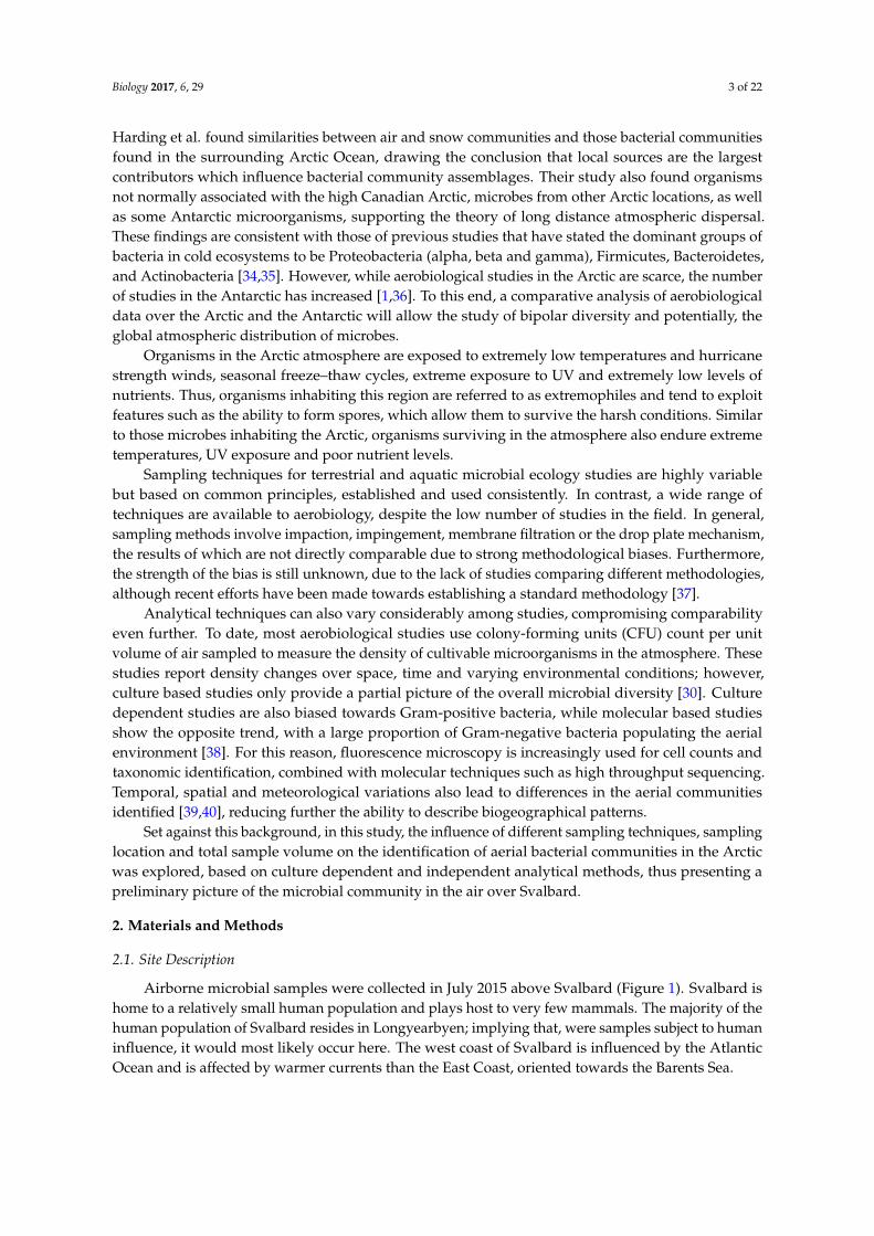
Airborne microbial samples were collected in July 2015 above Svalbard (Figure 1). Svalbard ishome to a relatively small human population and plays host to very few mammals. The majority of thehuman population of Svalbard resides in Longyearbyen; implying that, were samples subject to humaninfluence, it would most likely occur here. The west coast of Svalbard is influenced by the AtlanticOcean and is affected by warmer currents than the East Coast, oriented towards the Barents Sea.

Biology 2017, 6, 29 4 of 22Biology 2017, 6, 29 4 of 21

Figure 1. Svalbard location and sampling sites (map adapted with courtesy of the © Norwegian Polar

Institute (http://www.npolar.no/no/).

Samples were collected between 6 and 23 July 2015 above both marine and terrestrial locations

using a range of techniques (Table 1). Marine samples were collected aboard the research ship (Viking

Explorer) and aboard a zodiac. The terrestrial sites were on the roof of The University Center in

Svalbard (UNIS (78°13′ N, 15°39′ E)) located in central Longyearbyen, Mine (Gruve) 7, Deltaneset,

Gipsdalen and Bjørndalen; these locations were chosen to represent a large terrestrial geographic

range. The marine sites were located in the surrounding fjords at Billefjorden, Isfjorden,

Sassenfjorden and Adventfjorden bay (Figure 1).

Table 1. Summary of sample locations and regimes.

Sample

Location Environment Sampling Mechanism Date

Flow Rate

(L m−1) Duration (min)

Bjørndalen Terrestrial Drop plates 13 July 2015 - 15

Deltaneset Terrestrial Impaction onto media 13 July 2015 50 20

Drop plates 13 July 2015 - 15

Gipsdalen Terrestrial Impaction onto media 13 July 2015 50 20

Drop plates 13 July 2015 - 15

Longyearbyen Terrestrial Impaction onto media 16 July 2015 30, 50 20, 40, 60, 80

Membrane filtration 06, 19, 21–23 July

2015 ~20 30, 60, 120, 300, 3 days

Mine (Gruve) 7 Terrestrial Impaction onto media 13 July 2015 50 20

Drop plates 13 July 2015 - 15

Adventfjorden Marine Impaction onto media 17 July 2015 50 20

Billefjorden Marine Impaction onto media 17 July 2015 50 20

Isfjorden Marine Membrane filtration 11 July 2015 ~20 480

Sassenfjorden Marine Impaction onto media 17 July 2015 50 20

2.2. Meteorological Data

Seven-day back trajectory models were calculated for sampling days where sequencing was

carried out at air mass arrival heights of 10 m, 500 m and 1500 m (Figure 2) using National Oceanic

and Atmospheric Administration (NOAA) Hysplit Model [41] and the Global Data Assimilation

System (GDAS1) archived data file. In general, pockets of air at all altitudes arrived from a northerly

(Arctic Ocean) direction, however high altitude air pockets at 1500 m were more easterly influenced

than the lower altitudes. On 6 July, the low altitude air masses (10 m, 500 m) were easterly.

Temperatures averaged 8 °C across all sampling days with only one precipitation event totalling 0.1

mm occurring on 17 July. Wind speed varied between 10 and 22 kmh-1 and humidity averaged 67%

(Table 2).

Figure 1. Svalbard location and sampling sites (map adapted with courtesy of the © Norwegian PolarInstitute (http://www.npolar.no/no/).

Samples were collected between 6 and 23 July 2015 above both marine and terrestrial locationsusing a range of techniques (Table 1). Marine samples were collected aboard the research ship (VikingExplorer) and aboard a zodiac. The terrestrial sites were on the roof of The University Center inSvalbard (UNIS (78◦13′ N, 15◦39′ E)) located in central Longyearbyen, Mine (Gruve) 7, Deltaneset,Gipsdalen and Bjørndalen; these locations were chosen to represent a large terrestrial geographic range.The marine sites were located in the surrounding fjords at Billefjorden, Isfjorden, Sassenfjorden andAdventfjorden bay (Figure 1).

Table 1. Summary of sample locations and regimes.

SampleLocation Environment Sampling Mechanism Date Flow Rate

(L m−1)Duration

(min)

Bjørndalen Terrestrial Drop plates 13 July 2015 - 15Deltaneset Terrestrial Impaction onto media 13 July 2015 50 20

Drop plates 13 July 2015 - 15Gipsdalen Terrestrial Impaction onto media 13 July 2015 50 20

Drop plates 13 July 2015 - 15Longyearbyen Terrestrial Impaction onto media 16 July 2015 30, 50 20, 40, 60, 80

Membrane filtration 06, 19, 21–23 July2015 ~20 30, 60, 120, 300,

3 daysMine (Gruve) 7 Terrestrial Impaction onto media 13 July 2015 50 20

Drop plates 13 July 2015 - 15Adventfjorden Marine Impaction onto media 17 July 2015 50 20

Billefjorden Marine Impaction onto media 17 July 2015 50 20Isfjorden Marine Membrane filtration 11 July 2015 ~20 480

Sassenfjorden Marine Impaction onto media 17 July 2015 50 20

2.2. Meteorological Data

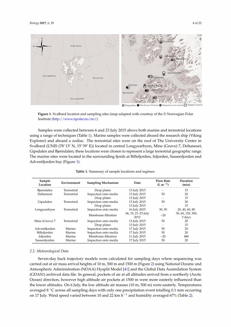
Seven-day back trajectory models were calculated for sampling days where sequencing wascarried out at air mass arrival heights of 10 m, 500 m and 1500 m (Figure 2) using National Oceanic andAtmospheric Administration (NOAA) Hysplit Model [41] and the Global Data Assimilation System(GDAS1) archived data file. In general, pockets of air at all altitudes arrived from a northerly (ArcticOcean) direction, however high altitude air pockets at 1500 m were more easterly influenced thanthe lower altitudes. On 6 July, the low altitude air masses (10 m, 500 m) were easterly. Temperaturesaveraged 8 ◦C across all sampling days with only one precipitation event totalling 0.1 mm occurringon 17 July. Wind speed varied between 10 and 22 km h−1 and humidity averaged 67% (Table 2).

Biology 2017, 6, 29 5 of 22Biology 2017, 6, 29 5 of 21

Figure 2. Back trajectory models were calculated using the NOAA Hysplit Model [41]. Three arrival

heights were used 10 m (transect marked by triangles), 500 m (transect marked with squares) and

1500 m (transects marked with circles). Sampling location is marked by a black star.

Table 2. Meteorological conditions on sampling days at Svalbard airport (The Weather Company

(Atlanta, GA, USA)).

06 July

2015

11 July

2015

13 July

2015

16 July

2015

17 July

2015

19 July

2015

21 July

2015

22 July

2015

23 July

2015

21–23 July

2015

(Average)

Average across All

Sampling Days

Average

temperature

(°C)

8 10 8 6 8 8 10 8 6 8 8

Total

precipitation

(mm)

0 0 0 0 0.1 0 0 0 0 0 0

Average wind

speed (kmh-1) 13 20 10 20 14 22 18 12 12 14 16

Figure 2. Back trajectory models were calculated using the NOAA Hysplit Model [41]. Three arrivalheights were used 10 m (transect marked by triangles), 500 m (transect marked with squares) and1500 m (transects marked with circles). Sampling location is marked by a black star.

Biology 2017, 6, 29 6 of 22

Table 2. Meteorological conditions on sampling days at Svalbard airport (The Weather Company (Atlanta, GA, USA)).

06 July 2015 11 July 2015 13 July 2015 16 July 2015 17 July 2015 19 July 2015 21 July 2015 22 July 2015 23 July 2015 21–23 July 2015(Average)

Average across AllSampling Days

Average temperature (◦C) 8 10 8 6 8 8 10 8 6 8 8Total precipitation (mm) 0 0 0 0 0.1 0 0 0 0 0 0

Average wind speed (km h−1) 13 20 10 20 14 22 18 12 12 14 16Average humidity (%) 63 75 90 57 68 59 65 68 61 65 67

Pressure (hPa) 1025 1022 1019 1009 1013 1015 1015 1013 1006 1012 1016

Biology 2017, 6, 29 7 of 22

2.3. Culture Dependent

Drop plates containing R2A media (Sigma-Aldrich, St. Louis, MO, USA) were placed open atGipsdalen, Mine (Gruve) 7, Deltaneset and Bjørndalen for 15 min; plates were incubated for 10 days atroom temperature; following incubation the plates had colony counts and distinct colony counts taken.

Additionally, a portable AirPort MD8 (Sartorius, Göttingen, Germany), comprising a disposablegelatine filter membrane, was used to compare sampling efficiency and cultivability at two flowrates and different sampling volumes. Sampling sites were chosen to compare with terrestrial platedrop sites but also to assess for the differences at marine sites. Terrestrial samples were collected atMine (Gruve) 7, Deltaneset, Gipsdalen and central Longyearbyen (UNIS roof) and marine samples atBillefjorden, Sassenfjorden and Adventfjorden, respectively. The sampler was used at respective flowrates and durations ranging 30–50 L m−1 and 20–80 L m−1 on 13, 15, 16 and 17 July 2015. The gelatinefilters collected at all sites were placed directly onto the surface of R2A agar plates (Sigma-Aldrich,St. Louis, MO, USA). These plates were then incubated at room temperature for 10 days. Total CFUand distinct colony numbers were counted.

2.4. Culture Independent

As gelatine filters are not amenable to culture independent techniques (due to the presenceof gelatine), airborne bacteria from both terrestrial and marine sites were collected via membranefiltration. A Welch WOB-L vacuum pump (Welch, Mt. Prospect, IL, USA) was set up at a flow rate of~20 L m−1 connected to Sartorius filtration unit (Göttingen, Germany) containing a 47 mm × 0.2 µmpore size cellulose nitrate membrane filter (GE Healthcare Life Sciences, Chicago, IL, USA).

A marine sample was collected at Isfjorden on the 11 July 2015 with a respective sample durationand volume of 8 h and ~9600 L and the terrestrial sample was taken in central Longeyearbyen (UNISroof) at the following dates, durations and volumes, respectively: 6 July 2015 for 30 (600 L), 60 (1200 L),120 (2400 L) and 300 (6000 L) min; 19 July 2015 for 30 (600 L), 60 (1200 L), 120 (2400 L) and 300 (6000 L)min; and 21–24 July 2015 for three days (~86,000 L) continuously (Table 1).

The cellulose nitrate membrane filters were sent to MrDNA (MrDRNA, Shallowater, TX, USA) forextraction and sequencing. DNA was extracted from samples using the MoBio PowerSoil kit (MoBio,Vancouver, BC, Canada) following the manufacturer’s protocol with an additional 1 min of beadbeating to account for the filter paper. Extracted samples were then amplified using 16S rRNA universalprimers 27Fmod (AGRGTTTGATCMTGGCTCAG) and 519Rmodbio (GWATTACCGCGGCKGCTG)and barcodes were attached at the 5′ end. A 28-cycle PCR using the HotStarTaq Plus Master Mix Kit(Qiagen, Germantown, MD, USA) was carried out under the following conditions: 94 ◦C for 3 min,followed by 28 cycles of 94 ◦C for 30 s, 53 ◦C for 40 s and 72 ◦C for 1 min, after which a final elongationstep at 72 ◦C for 5 min was performed. After amplification, PCR products were checked in 2% agarosegel to determine amplification success. Samples were then pooled based on their molecular weight andDNA concentrations, purified and illumina DNA libraries were prepared. Paired end sequencing ofthe V4 region was then performed on a MiSeq following the manufacturer’s guidelines. The resultantdata were analysed using QIIME v1.9.1 [42]. The 776,315 raw sequence reads were quality trimmedand checked for chimeras using USEARCH 6.1 [43], clustered at an identity threshold of 97% andassigned to Operational Taxonomic Units (OTUs) using UCLUST [43] and the Greengenes referencedatabase [44] was used to assign taxonomy. Sequences were then aligned using PyNAST [45] and aphylogenetic tree was built using FastTree [46].

2.5. Statistical Analysis

Statistical analyses were performed using PAST [47] to test for differences in means, medians,variances and distributions and MS Excel (2013) to calculate correlation coefficients, the coefficient ofvariance and produce graphs of the analyses; statistical tests were carried out at an assumed significanceof alpha: 0.05. When calculating diversity indices, to avoid statistical bias due to differences in

Biology 2017, 6, 29 8 of 22

sequencing depth all samples were normalised to a depth of 26,190 reads. Rarefaction curves, diversityindices (Shannon and Simpsons reciprocal), Bray-Curtis OTU and unweighted UniFrac phylogeneticdistance metrics, and PCoAs were produced using QIIME [42].

3. Results

3.1. Culture Dependent

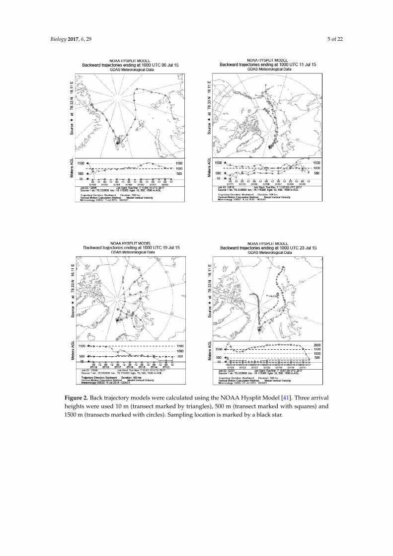
Viable bacteria were found in all of the samples. Clear differences were apparent in the mean CFUsfrom the two culture dependent methods used (Figure 3). A Kruskal–Wallis test for equal medians ofCFUs and morphologically distinct CFUs was undertaken to assess the drop plate replicates, the resultdid not show significant differences (Kruskal–Wallis plate fall CFU: p = 0.095, plate fall morphologicallydistinct CFUs: p = 0.123).

Biology 2017, 6, 29 7 of 21

2.5. Statistical Analysis

Statistical analyses were performed using PAST [47] to test for differences in means, medians,

variances and distributions and MS Excel (2013) to calculate correlation coefficients, the coefficient of

variance and produce graphs of the analyses; statistical tests were carried out at an assumed

significance of alpha: 0.05. When calculating diversity indices, to avoid statistical bias due to

differences in sequencing depth all samples were normalised to a depth of 26,190 reads. Rarefaction

curves, diversity indices (Shannon and Simpsons reciprocal), Bray–Curtis OTU and unweighted

UniFrac phylogenetic distance metrics, and PCoAs were produced using QIIME [42].

3. Results

3.1. Culture Dependent

Viable bacteria were found in all of the samples. Clear differences were apparent in the mean

CFUs from the two culture dependent methods used (Figure 3). A Kruskal–Wallis test for equal

medians of CFUs and morphologically distinct CFUs was undertaken to assess the drop plate

replicates, the result did not show significant differences (Kruskal–Wallis plate fall CFU: p = 0.095,

plate fall morphologically distinct CFUs: p = 0.123).

Figure 3. Mean colony-forming units (CFU) and morphologically distinct CFU counts for drop plate

and Sartorius MD8 data.

Comparing the differences in drop plate and MD8 results for the locations where data were

available for both methods, the MD8 showed much higher CFU yields, although this difference is not

obvious when looking at the number of morphologically distinct CFUs i.e. CFUs of different

appearance (Figure 3). Statistical analyses show a significant difference of mean CFUs sampled at the

same location using different methods (p < 0.05); no differences in variances, medians or coefficient

of variations, but a significant difference in equality of distributions (Kolmogov–Smirnov: p < 0.05).

For the morphologically distinct CFUs, however, there were no significant differences for any of the

mentioned parameters. When looking at the overall variance and efficiency of both culture dependent

Figure 3. Mean colony-forming units (CFU) and morphologically distinct CFU counts for drop plateand Sartorius MD8 data.

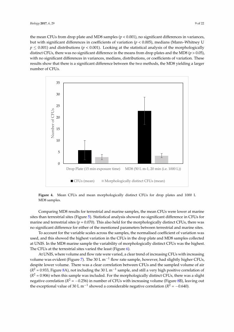
Comparing the differences in drop plate and MD8 results for the locations where data wereavailable for both methods, the MD8 showed much higher CFU yields, although this difference isnot obvious when looking at the number of morphologically distinct CFUs i.e., CFUs of differentappearance (Figure 3). Statistical analyses show a significant difference of mean CFUs sampled at thesame location using different methods (p < 0.05); no differences in variances, medians or coefficientof variations, but a significant difference in equality of distributions (Kolmogov–Smirnov: p < 0.05).For the morphologically distinct CFUs, however, there were no significant differences for any of thementioned parameters. When looking at the overall variance and efficiency of both culture dependentmethods, only considering the MD8 samples collected at 50 L m−1 for 20 min i.e., 1000 L samplingvolume (Figure 4), there were obvious differences in the mean CFUs, but not for morphologicallydistinct CFUs. An independent t-test comparing the two methods showed a significant difference in

Biology 2017, 6, 29 9 of 22

the mean CFUs from drop plate and MD8 samples (p < 0.001), no significant differences in variances,but with significant differences in coefficients of variation (p < 0.005), medians (Mann–Whitney Up ≤ 0.001) and distributions (p < 0.001). Looking at the statistical analysis of the morphologicallydistinct CFUs, there was no significant difference in the means from drop plates and the MD8 (p > 0.05),with no significant differences in variances, medians, distributions, or coefficients of variation. Theseresults show that there is a significant difference between the two methods, the MD8 yielding a largernumber of CFUs.

Biology 2017, 6, 29 8 of 21

methods, only considering the MD8 samples collected at 50 L m−1 for 20 min i.e., 1000 L sampling

volume (Figure 4), there were obvious differences in the mean CFUs, but not for morphologically

distinct CFUs. An independent t-test comparing the two methods showed a significant difference in

the mean CFUs from drop plate and MD8 samples (p < 0.001), no significant differences in variances,

but with significant differences in coefficients of variation (p < 0.005), medians (Mann–Whitney U p

≤ 0.001) and distributions (p < 0.001). Looking at the statistical analysis of the morphologically

distinct CFUs, there was no significant difference in the means from drop plates and the MD8 (p >

0.05), with no significant differences in variances, medians, distributions, or coefficients of variation.

These results show that there is a significant difference between the two methods, the MD8 yielding

a larger number of CFUs.

Figure 4. Mean CFUs and mean morphologically distinct CFUs for drop plates and 1000 L MD8

samples.

Comparing MD8 results for terrestrial and marine samples, the mean CFUs were lower at marine

sites than terrestrial sites (Figure 5). Statistical analysis showed no significant difference in CFUs for

marine and terrestrial sites (p = 0.070). This also held for the morphologically distinct CFUs, there was

no significant difference for either of the mentioned parameters between terrestrial and marine sites.

To account for the variable scales across the samples, the normalised coefficient of variation was

used, and this showed the highest variation in the CFUs in the drop plate and MD8 samples collected

at UNIS. In the MD8 marine sample the variability of morphologically distinct CFUs was the highest.

The CFUs at the terrestrial sites varied the least (Figure 6).

At UNIS, where volume and flow rate were varied, a clear trend of increasing CFUs with

increasing volume was evident (Figure 7). The 30 L m−1 flow rate sample, however, had slightly

higher CFUs, despite lower volume. There was a clear correlation between CFUs and the sampled

volume of air (R² = 0.933, Figure 8A), not including the 30 L m−1 sample, and still a very high positive

correlation of (R² = 0.906) when this sample was included. For the morphologically distinct CFUs,

there was a slight negative correlation (R² = −0.256) in number of CFUs with increasing volume

(Figure 8B), leaving out the exceptional value of 30 L m−1 showed a considerable negative correlation

(R² = −0.640).

0

5

10

15

20

25

30

35

Drop Plate (15 min exposure time) MD8 (50 L m-1, 20 min (i.e. 1000 L))

Nu

mb

er o

f C

FU

s

CFUs (mean) Morphologically distinct CFUs (mean)

Figure 4. Mean CFUs and mean morphologically distinct CFUs for drop plates and 1000 LMD8 samples.

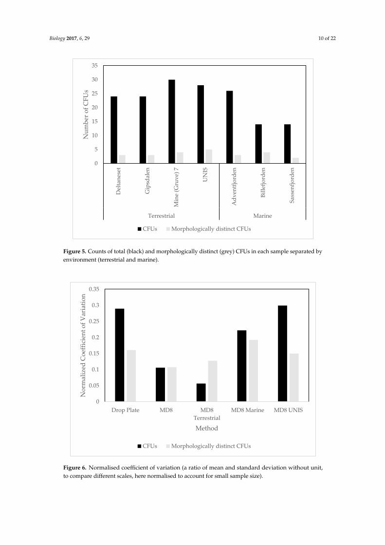
Comparing MD8 results for terrestrial and marine samples, the mean CFUs were lower at marinesites than terrestrial sites (Figure 5). Statistical analysis showed no significant difference in CFUs formarine and terrestrial sites (p = 0.070). This also held for the morphologically distinct CFUs, there wasno significant difference for either of the mentioned parameters between terrestrial and marine sites.

To account for the variable scales across the samples, the normalised coefficient of variation wasused, and this showed the highest variation in the CFUs in the drop plate and MD8 samples collectedat UNIS. In the MD8 marine sample the variability of morphologically distinct CFUs was the highest.The CFUs at the terrestrial sites varied the least (Figure 6).

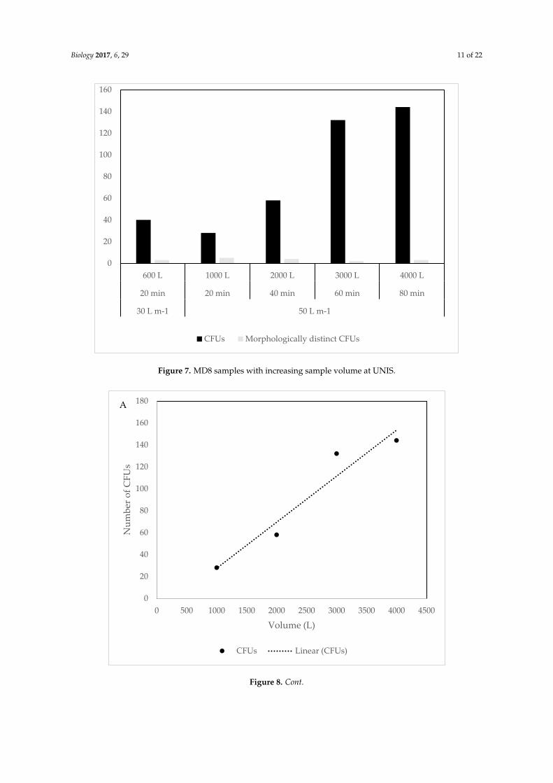
At UNIS, where volume and flow rate were varied, a clear trend of increasing CFUs with increasingvolume was evident (Figure 7). The 30 L m−1 flow rate sample, however, had slightly higher CFUs,despite lower volume. There was a clear correlation between CFUs and the sampled volume of air(R2 = 0.933, Figure 8A), not including the 30 L m−1 sample, and still a very high positive correlation of(R2 = 0.906) when this sample was included. For the morphologically distinct CFUs, there was a slightnegative correlation (R2 = −0.256) in number of CFUs with increasing volume (Figure 8B), leaving outthe exceptional value of 30 L m−1 showed a considerable negative correlation (R2 = −0.640).

Biology 2017, 6, 29 10 of 22

Biology 2017, 6, 29 9 of 21

Figure 5. Counts of total (black) and morphologically distinct (grey) CFUs in each sample separated

by environment (terrestrial and marine).

Figure 6. Normalised coefficient of variation (a ratio of mean and standard deviation without unit, to

compare different scales, here normalised to account for small sample size).

0

5

10

15

20

25

30

35

Del

tan

eset

Gip

sdal

en

Min

e (G

ruv

e) 7

UN

IS

Ad

ven

tfjo

rden

Bil

lefj

ord

en

Sas

sen

fjo

rden

Terrestrial Marine

Nu

mb

er o

f C

FU

s

CFUs Morphologically distinct CFUs

0

0.05

0.1

0.15

0.2

0.25

0.3

0.35

Drop Plate MD8 MD8

Terrestrial

MD8 Marine MD8 UNIS

No

rmal

ized

Co

effi

cien

t o

f V

aria

tio

n

Method

CFUs Morphologically distinct CFUs

Figure 5. Counts of total (black) and morphologically distinct (grey) CFUs in each sample separated byenvironment (terrestrial and marine).

Biology 2017, 6, 29 9 of 21

Figure 5. Counts of total (black) and morphologically distinct (grey) CFUs in each sample separated

by environment (terrestrial and marine).

Figure 6. Normalised coefficient of variation (a ratio of mean and standard deviation without unit, to

compare different scales, here normalised to account for small sample size).

0

5

10

15

20

25

30

35

Del

tan

eset

Gip

sdal

en

Min

e (G

ruv

e) 7

UN

IS

Ad

ven

tfjo

rden

Bil

lefj

ord

en

Sas

sen

fjo

rden

Terrestrial Marine

Nu

mb

er o

f C

FU

s

CFUs Morphologically distinct CFUs

0

0.05

0.1

0.15

0.2

0.25

0.3

0.35

Drop Plate MD8 MD8

Terrestrial

MD8 Marine MD8 UNIS

No

rmal

ized

Co

effi

cien

t o

f V

aria

tio

n

Method

CFUs Morphologically distinct CFUs

Figure 6. Normalised coefficient of variation (a ratio of mean and standard deviation without unit,to compare different scales, here normalised to account for small sample size).

Biology 2017, 6, 29 11 of 22

Biology 2017, 6, 29 10 of 21

Figure 7. MD8 samples with increasing sample volume at UNIS.

0

20

40

60

80

100

120

140

160

600 L 1000 L 2000 L 3000 L 4000 L

20 min 20 min 40 min 60 min 80 min

30 L m-1 50 L m-1

CFUs Morphologically distinct CFUs

0

20

40

60

80

100

120

140

160

180

0 500 1000 1500 2000 2500 3000 3500 4000 4500

Nu

mb

er o

f C

FU

s

Volume (L)

CFUs Linear (CFUs)

A

Figure 7. MD8 samples with increasing sample volume at UNIS.

Biology 2017, 6, 29 10 of 21

Figure 7. MD8 samples with increasing sample volume at UNIS.

0

20

40

60

80

100

120

140

160

600 L 1000 L 2000 L 3000 L 4000 L

20 min 20 min 40 min 60 min 80 min

30 L m-1 50 L m-1

CFUs Morphologically distinct CFUs

0

20

40

60

80

100

120

140

160

180

0 500 1000 1500 2000 2500 3000 3500 4000 4500

Nu

mb

er o

f C

FU

s

Volume (L)

CFUs Linear (CFUs)

A

Figure 8. Cont.

Biology 2017, 6, 29 12 of 22

Biology 2017, 6, 29 11 of 21

Figure 8. (A) CFUs sampled against total volume of air (excluding 30 L m−1 sample). (B) CFUs sampled

against total volume of air (all samples).

3.2. Culture Independent

3.2.1. Bacterial Diversity

Targeted amplicon sequencing of the 16S rRNA V4 region resulted in 776,315 total reads across

the 10 samples, which were then quality filtered and checked for chimeras leaving 685,583 reads. The

range of reads per sample ranged from 32,651 (recorded in the 60 min sample from 6 July) to 145,488

reads (recordedin the 30 min sample collected on 19 July). Samples were then rarefied to 26,190 reads

(lower than the smallest sample); rarefied samples averaged 5015 OTUs (range 4143–6402).

Rarefaction curves for all of the normalised samples did not reach asymptote suggesting the full

extent of the diversity present was not reached for all samples (Figure 9A). The Shannon diversity

index, a proxy for richness and evenness, was similar in all samples (Figure 9B). The results showed

that all samples shared similar levels of diversity (Shannon index range 7.66–9.28); the most diverse

sample based on the Shannon index was the 30 min sample taken on Day 2 whilst the least diverse

sample based on this metric was the 60 min sample on Day 1. The dominance Simpsons reciprocal

index showed a larger difference in the degree of diversity between samples, showing the marine

sample to be the most diverse with a Simpsons reciprocal value of 114.13 whilst the lowest diversity

was seen again in the Day 1 60 min sample with a value of 20.35 (Figure 9C).

The differences in OTU diversity between the communities was measured using the Bray–Curtis

dissimilarity index (Figure 10A) and an un-weighted UniFrac was used to estimate the phylogenetic

distance between different communities (Figure 10B), the variation across all PCoA axis was low.

Both metrics showed no distinct pattern between sampling days; however, sampling location did

have an effect and different sampling durations showed minor clustering between the 60 and 120 min

durations on Day 1. All samples reported differing levels of richness and evenness (Figure 10A) and

showed considerable phylogenetic distances with the greatest distance in the three-day sample

(Figure 10B).

0

1

2

3

4

5

6

0 500 1000 1500 2000 2500 3000 3500 4000 4500

Nu

mb

er o

f M

orp

ho

log

ical

ly d

isti

nct

CF

Us

Volume (L)

Morphologically distinct CFUs

Linear (Morphologically distinct CFUs)

B

Figure 8. (A) CFUs sampled against total volume of air (excluding 30 L m−1 sample). (B) CFUssampled against total volume of air (all samples).

3.2. Culture Independent

3.2.1. Bacterial Diversity

Targeted amplicon sequencing of the 16S rRNA V4 region resulted in 776,315 total reads acrossthe 10 samples, which were then quality filtered and checked for chimeras leaving 685,583 reads.The range of reads per sample ranged from 32,651 (recorded in the 60 min sample from 6 July) to145,488 reads (recordedin the 30 min sample collected on 19 July). Samples were then rarefied to26,190 reads (lower than the smallest sample); rarefied samples averaged 5015 OTUs (range 4143–6402).Rarefaction curves for all of the normalised samples did not reach asymptote suggesting the full extentof the diversity present was not reached for all samples (Figure 9A). The Shannon diversity index,a proxy for richness and evenness, was similar in all samples (Figure 9B). The results showed that allsamples shared similar levels of diversity (Shannon index range 7.66–9.28); the most diverse samplebased on the Shannon index was the 30 min sample taken on Day 2 whilst the least diverse samplebased on this metric was the 60 min sample on Day 1. The dominance Simpsons reciprocal indexshowed a larger difference in the degree of diversity between samples, showing the marine sample tobe the most diverse with a Simpsons reciprocal value of 114.13 whilst the lowest diversity was seenagain in the Day 1 60 min sample with a value of 20.35 (Figure 9C).

The differences in OTU diversity between the communities was measured using the Bray-Curtisdissimilarity index (Figure 10A) and an un-weighted UniFrac was used to estimate the phylogeneticdistance between different communities (Figure 10B), the variation across all PCoA axis was low. Bothmetrics showed no distinct pattern between sampling days; however, sampling location did have aneffect and different sampling durations showed minor clustering between the 60 and 120 min durationson Day 1. All samples reported differing levels of richness and evenness (Figure 10A) and showedconsiderable phylogenetic distances with the greatest distance in the three-day sample (Figure 10B).

Biology 2017, 6, 29 13 of 22Biology 2017, 6, 29 12 of 21

Figure 9. α-Diversity measures: (A) Rarefaction curves for observed species; (B) Shannon index; and

(C) Simpsons reciprocal index.

Figure 10. Jackknifed β-diversity metrics: (A) Bray–Curtis Index; and (B) Unweighted UniFrac.

3.2.2. Taxonomy

Twelve phyla in total were detected within the samples: Proteobacteria, Firmicutes and

Actinobacteria were present in all of the samples at differing but high relative abundances and were

the visibly dominant phyla (Figure 11); Bacteroidetes, Chloroflexi and Cyanobacteria were also

present in all samples; and Cyanobacteria and Bacteroidetes were present in sporadically large

relative abundances, however, in general, these three phyla were present at <1% (Figure 11).

Figure 9. α-Diversity measures: (A) Rarefaction curves for observed species; (B) Shannon index; and(C) Simpsons reciprocal index.

PC2 (12.66%)

PC3 (11.93%) PC1 (13.29%)

Isfjorden, 8 hours

UNIS day 1, 30 minutes

UNIS day 2, 30 minutes

A BUNIS, 3 days

UNIS day 1, 60 minutesUNIS day 1, 120 minutes

UNIS day 1, 300 minutes

UNIS day 2, 60 minutes

UNIS day 2, 300 minutes

PC2 (15.43%)

PC3 (13.74%)

PC1 (18.38%)

UNIS day 2, 60 minutes

UNIS day 1, 300 minutes

UNIS day 2, 300 minutesUNIS day 2, 120 minutes

UNIS day 1, 60 minutes

UNIS, 3 days

UNIS day 1, 120 minutes

Isfjorden, 8 hours

UNIS day 1, 30 minutes

UNIS day 1, 60 minutes

UNIS day 2, 120 minutes

Figure 10. Jackknifed β-diversity metrics: (A) Bray-Curtis Index; and (B) Unweighted UniFrac.

3.2.2. Taxonomy

Twelve phyla in total were detected within the samples: Proteobacteria, Firmicutes andActinobacteria were present in all of the samples at differing but high relative abundances andwere the visibly dominant phyla (Figure 11); Bacteroidetes, Chloroflexi and Cyanobacteria were alsopresent in all samples; and Cyanobacteria and Bacteroidetes were present in sporadically large relativeabundances, however, in general, these three phyla were present at <1% (Figure 11).

Biology 2017, 6, 29 14 of 22

Biology 2017, 6, 29 13 of 21

Figure 11. Phyla level relative abundances (%) of bacteria in all culture independent samples.

Proteobacteria, Firmicutes and Actinobacteria represented ~99% of the Day 1 sample set in

which there were 10 phyla present in total (Figure 11). Proteobacteria showed the largest total and

range of relative abundance on this sampling day. On Day 2, there were 12 phyla present.

Proteobacteria, Firmicutes and Actinobacteria remained the three key phyla at a total average relative

abundance of 75%. The decrease in relative abundance from Day 1 was mirrored in the 60 and 300

min duration samples by an increase in the average relative abundance of Bacteroidetes. The three-

day sample contained 10 phyla as for Day 1, but showed similar phyla and relative abundances to

the 60 min sample on Day 2. Acidobacteria were present at 6% in this sample, but they were present

at <1% relative abundance in all other samples. The marine sample collected at Isfjorden contained

10 distinct phyla, the same number present in the Day 1 and three-day sample.

There were 196 genera in total, 58 of which were present in all samples. The marine sample taken

at Isfjorden contained the highest number of distinct genera with 148, whilst the terrestrial 120 min

sample on Day 2 contained the lowest number of genera at 100. On Day 1, the average number of

genera present was 190 whilst on Day 2 the number dropped to 113. In the three-day sample at UNIS

there were 130 genera, more than in any of the other eight samples collected at that location.

Pseudomonas, Staphylococcus, Propionibacterium, Delftia and Corynebacterium spp. made up the five

most relatively abundant genera. Pseudomonas was the most common and relatively abundant genera

representing 18% of the full sample set, however, they were only the most abundant genera in the

Day 1, 30 min sample. Pseudomonas, Acinetobacter, Corynebacterium, Staphylococcus, Deltia,

Cloacibacterium, Arthrobacter, Sphingomonas, Alcanivorax, Comamonas, Streptomyces and Brevibacterium

spp. were all regularly present in the top 10 most abundant genera in each sample (Table 3). Members

of the order Lactobacillales and Alcaligenes were both present in all four Day 1 samples but just one

Day 2 samples whilst Microbacterium, a genus of the Microbacteriaceae family and a member of the

Intrasporangiaceae family were present in all four Day 2 samples but just one Day 1 sample. There

were 15 genera specific to Day 1 and 17 specific to Day 2. The three-day sample recorded six genera

specific to that sample. The marine sample recorded the highest number of sample specific genera

with 17.

0%

10%

20%

30%

40%

50%

60%

70%

80%

90%

100%

UNIS day 1,

30 minutes

UNIS day 1,

60 minutes

UNIS day 1,

120 minutes

UNIS day 1,

300 minutes

UNIS day 2,

30 minutes

UNIS day 2,

60 minutes

UNIS day 2,

120 minutes

UNIS day 2,

300 minutes

UNIS, 3 days Isfjorden, 8

hours

Rel

ativ

e ab

un

dan

ce

Sample

Verrucomicrobia

Tenericutes

TM7

Proteobacteria

GN04

Firmicutes

Cyanobacteria

Chloroflexi

Bacteroidetes

Actinobacteria

Acidobacteria

AD3

Other

Unassigned

Figure 11. Phyla level relative abundances (%) of bacteria in all culture independent samples.

Proteobacteria, Firmicutes and Actinobacteria represented ~99% of the Day 1 sample set in whichthere were 10 phyla present in total (Figure 11). Proteobacteria showed the largest total and rangeof relative abundance on this sampling day. On Day 2, there were 12 phyla present. Proteobacteria,Firmicutes and Actinobacteria remained the three key phyla at a total average relative abundance of75%. The decrease in relative abundance from Day 1 was mirrored in the 60 and 300 min durationsamples by an increase in the average relative abundance of Bacteroidetes. The three-day samplecontained 10 phyla as for Day 1, but showed similar phyla and relative abundances to the 60 minsample on Day 2. Acidobacteria were present at 6% in this sample, but they were present at <1%relative abundance in all other samples. The marine sample collected at Isfjorden contained 10 distinctphyla, the same number present in the Day 1 and three-day sample.

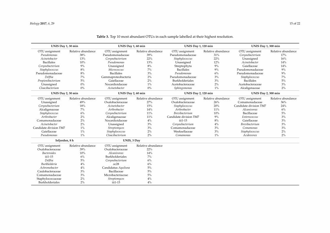
There were 196 genera in total, 58 of which were present in all samples. The marine sampletaken at Isfjorden contained the highest number of distinct genera with 148, whilst the terrestrial120 min sample on Day 2 contained the lowest number of genera at 100. On Day 1, the average numberof genera present was 190 whilst on Day 2 the number dropped to 113. In the three-day sample atUNIS there were 130 genera, more than in any of the other eight samples collected at that location.Pseudomonas, Staphylococcus, Propionibacterium, Delftia and Corynebacterium spp. made up the fivemost relatively abundant genera. Pseudomonas was the most common and relatively abundant generarepresenting 18% of the full sample set, however, they were only the most abundant genera in the Day 1,30 min sample. Pseudomonas, Acinetobacter, Corynebacterium, Staphylococcus, Deltia, Cloacibacterium,Arthrobacter, Sphingomonas, Alcanivorax, Comamonas, Streptomyces and Brevibacterium spp. were allregularly present in the top 10 most abundant genera in each sample (Table 3). Members of the orderLactobacillales and Alcaligenes were both present in all four Day 1 samples but just one Day 2 sampleswhilst Microbacterium, a genus of the Microbacteriaceae family and a member of the Intrasporangiaceaefamily were present in all four Day 2 samples but just one Day 1 sample. There were 15 genera specificto Day 1 and 17 specific to Day 2. The three-day sample recorded six genera specific to that sample.The marine sample recorded the highest number of sample specific genera with 17.

Biology 2017, 6, 29 15 of 22

Table 3. Top 10 most abundant OTUs in each sample labelled at their highest resolution.

UNIS Day 1, 30 min UNIS Day 1, 60 min UNIS Day 1, 120 min UNIS Day 1, 300 min

OTU assignment Relative abundance OTU assignment Relative abundance OTU assignment Relative abundance OTU assignment Relative abundancePseudomonas 38% Pseudomonadaceae 39% Pseudomonadaceae 31% Corynebacterium 17%Acinetobacter 13% Corynebacterium 22% Staphylococcus 22% Unassigned 16%

Bacillales 10% Pseudomonas 13% Unassigned 12% Acinetobacter 14%Corynebacterium 9% Unassigned 8% Streptophyta 9% Gaiellaceae 14%Staphylococcus 8% Micrococcus 7% Bacillales 9% Pseudomonadaceae 9%

Pseudomonadaceae 8% Bacillales 3% Pseudomonas 6% Pseudomonadaceae 9%Delftia 7% Gammaproteobacteria 2% Pseudomonadaceae 3% Staphylococcus 7%

Propionibacterium 5% Gaiellaceae 2% Burkholderiales 3% Bacillales 5%Unassigned 0% Nocardioidaceae 1% Acetobacteraceae 2% Acetobacteraceae 3%

Cloacibacterium 0% Acinetobacter 0% Sphingomonas 1% Alcaligenaceae 2%

UNIS Day 2, 30 min UNIS Day 2, 60 min UNIS Day 2, 120 min UNIS Day 2, 300 min

OTU assignment Relative abundance OTU assignment Relative abundance OTU assignment Relative abundance OTU assignment Relative abundanceUnassigned 49% Oxalobacteraceae 27% Oxalobacteraceae 26% Comamonadaceae 36%

Corynebacterium 18% Acinetobacter 15% Staphylococcus 20% Candidate division TM7 24%Alcaligenaceae 7% Arthrobacter 14% Arthrobacter 11% Alcanivorax 6%Staphylococcus 6% Corynebacterium 11% Brevibacterium 10% Bacillaceae 5%Arthrobacter 2% Alcaligenaceae 11% Candidate division TM7 9% Enterococcus 3%

Comamonadaceae 2% Nocardioidaceae 4% iii1-15 8% Gaiellaceae 3%Acinetobacter 2% Unassigned 3% Corynebacterium 4% Brevibacterium 3%

Candidate division TM7 1% Streptomyces 3% Comamonadaceae 3% Comamonas 3%Gaiellaceae 1% Staphylococcus 2% Weeksellaceae 3% Staphylococcus 2%Pseudomonas 1% Cloacibacterium 2% Comamonas 1% Acidovorax 2%

Isfjorden, 8 h UNIS, 3 Day

OTU assignment Relative abundance OTU assignment Relative abundanceOxalobacteraceae 39% Oxalobacteraceae 22%

Bacteroides 10% Alcanivorax 14%iii1-15 6% Burkholderiales 7%Delftia 5% Corynebacterium 6%

Burkholderia 4% oc28 6%Achromobacter 4% Candidatus Aquiluna 5%

Caulobacteraceae 3% Bacillaceae 5%Comamonadaceae 3% Microbacteriaceae 5%Staphylococcaceae 2% Streptomyces 4%

Burkholderiales 2% iii1-15 4%

Biology 2017, 6, 29 16 of 22

4. Discussion

4.1. Culture Dependent

All culture dependent samples recorded growth, showing that viable microbes are common in theatmosphere, at both terrestrial and marine locations around Svalbard. The number of viable bacteriameasured in the air was considerably lower than the number measured in other environments e.g.,surface ice and cryoconite holes, where the number of CFU can be up to tenfold higher using the samemedia [48]. These results suggest that the atmosphere represents an extremely selective environment,although it is worth noting that only 0.2–2% of the culturable bacteria in the atmosphere are typicallyrecovered by culture dependent studies [49,50]. Previous studies using both drop plates and impactionbased techniques similar to the Sartorius MD8 have shown impaction to consistently produce moreCFUs [51], in line with this, the impaction method used here produced significantly higher CFUsoverall. At locations where both methods were employed, drop plates underestimated the number ofviable microbes compared to impaction, likely because a much higher volume of air is being activelydirected onto the collection plate using impaction. There was no significant (p > 0.05) difference in thenumber of morphologically distinct CFUs produced by the two methods, and none of them showedany particular bias for specific taxonomic groups on R2A. Replicates taken for drop plate samplesshowed the technique to be robust with no significant difference across the samples. Generally, marinestudies tend to present more CFUs than terrestrial samples [52]. Despite this, there were no significantdifferences between these two environments; although when normalising coefficients of variations inthe sample a clear difference was visible. In our case, the highest number of viable bacteria was in thesamples taken at UNIS, consistent with the diversity of activity in that location.

The number of cultivable bacteria increased with the increase in sample volume when usingthe MD8. This contradicts previous studies which showed no effect of sample volume on total CFUcounts [53]. In addition, decreasing the flow rate from 50 L m−1 to 30 L m−1 increased the numberof cultivable bacteria recovered, possibly due to the decreased impact stress placed on capturedbacteria [54].

Whilst culture dependent studies provide useful information about the proportion of viablebacteria in the atmosphere, it is generally considered that only around 1% of the total bacteria presentin the atmosphere are culturable [55]. Dormancy may represent an important survival mechanismfor bacteria in the atmosphere; therefore, a considerably larger proportion of viable non-culturablebacteria (VBNC) would also be expected and may have been overlooked in previous studies based onculture techniques alone. The reliance on CFU counts and inability to describe VBNC bacteria limitsthe value of culture dependent techniques from an ecological perspective.

4.2. Culture Independent

Culture independent studies using sequencing can provide more information about the diversityand taxonomic composition within an environment. Despite the ability of culture independent studiesto generate useful information, they also have major drawbacks, as they contain little informationabout the viability of the bacteria in the environment. Thus, combining both culture dependentand culture independent methods, provides a better insight into both the structure and viability ofbacterial communities.

Previous research on bacteria in the atmosphere outside the Arctic has linked temporal and spatialvariation to changes in the diversity and abundance [56]. Despite these factors impacting bacterialcommunities in other Arctic ecosystems such as soil [57], there are no studies to date which investigatethese patterns in the atmosphere in this region. Temporal variation (sampling day) did appear to havean effect on community structure, as the composition of the dominant Day 1 phyla was clearly differentto that on the other three sampling days. Spatial variation (marine and terrestrial) also appeared tohave an effect, although this was less pronounced than the temporal variation, as the dominant phylapresent in both the marine and terrestrial samples was consistent. Our results suggest that day of

Biology 2017, 6, 29 17 of 22

sampling (temporal) is more important than location (spatial) with regards to sample diversity mostlikely due to changes in meteorological conditions such as wind direction which appeared to producedistinct communities at the phylum level (Figure 11). Duration also appeared to have an effect on thetaxonomy of the communities, because whilst the dominant groups of phyla remained constant, therelative abundances varied considerably with changing duration. Although this variation could relateto confounding factors such as the time of day the samples were taken and the duration of sampling.

4.2.1. Diversity

Samples did not cluster into distinct groups based on OTU or phylogenetic relationships, showingno direct link between diversity and sampling duration, location or day (Figure 10A,B). On Day 1, 60and 120 min samples clustered based on both relationships, likely due to the samples sharing similarrelative abundances of Delftia, Ralstonia and Pseudomonas. A higher Simpson reciprocal value wasseen on the third sampling day (76.61) taken at UNIS, suggesting that sampling for a longer durationincreases the diversity of bacteria captured. The marine sample was considerably more diverse thanthe terrestrial samples when taking into account dominance (Figure 9C), further supporting the ideathat the distinct geographical features of marine coastal locations when compared to terrestrial onesgive rise to more varied communities [25,29]. Meteorological conditions such as wind speed, humidityand pressure are known to directly impact community structure [19]; however, during our study, theseconditions remained relatively constant, which could explain the similar levels of diversity of thesamples shown by the Shannon index (Figure 9B).

4.2.2. Taxonomy

A maximum of 12 phyla were found in air samples from Svalbard; however, the number ofphyla varied among samples. The pattern found on Day 1 was the most distinct with three phyladominating. The distinctiveness of the pattern on Day 1 was likely due to easterly winds from a lowaltitude air mass leading up to and during this sampling occasion. During the other sampling days,the predominant wind had a main westerly component. The 12 phyla could be separated into twogroups: the primary phyla Proteobacteria, Firmicutes and Actinobacteria; and the remaining phyla thatwere present in sporadic relative abundances. This pattern is consistent with previous studies in coldecosystems [23,26,34,35] and with bioaerosols from a range of environments [1,18,40,58]. Bacteroidetescould be considered a primary phyla, as they were present in considerable relative abundance inall of the samples apart from on Day 1, suggesting their source is to the east of Svalbard due tothe back trajectory of the prevailing wind direction. The primary phyla are probably well adaptedto atmospheric life, e.g., Firmicutes are well known for their ability to form spores in low nutrientconditions [59]. Actinobacteria have a higher GC content than other bacteria [60], which is a usefuldefence against the increased UV exposure faced by bioaerosols, and Proteobacteria are known to fill amultitude of niches due to the metabolic diversity of the group [61]. The number of phyla occurring inthe air above Svalbard is considerably lower than that described for urban environments, with studiesreporting the number of distinct phyla present to be as high as 38 [58], likely due to differences inthe environments. It is notable that Deinococcus sp. were not present in any of the samples, a groupof bacteria normally associated with atmospheric studies, both in the Artic and elsewhere [33,56].Bacillus sp. were responsible for a large proportion of the Firmicutes present in the sample, the sourceof which in the terrestrial samples was likely the surrounding soil [39]. There also appeared to be arelationship between the Actinobacteria and the Pseudomonadales whereby as the relative abundanceof one increased, the other decreased as has been found previously [62]. Interestingly there was a spikeof Acidobacteria in the three-day sample which could suggest this phyla is best adapted to survive thestress of desiccation caused by sampling for longer periods.

At the genus level, the patterns were much less distinct. Of the 196 genera, only 58 were present inall samples. The five most relatively abundant genera (Pseudomonas, Staphylococcus, Propionibacterium,Delftia and Corynebacterium spp.) are all either polar associated or ubiquitous. Delftia sp. have been

Biology 2017, 6, 29 18 of 22

described at multiple Arctic locations including Svalbard and Greenland where they are associatedwith surface ice [63,64] whilst Propionibacterium sp. are typically associated with marine sedimentin the Arctic Ocean [65,66]. Pseudomonas sp. are ubiquitous and present in almost all polar studies,however, on Svalbard they are mainly described from fjords [67]. Indeed, a new psychrophilic speciesof Pseudomonas was recently described from the same region [68]. Corynebacterium sp. have previouslybeen found in soils from the Canadian high Arctic [69]. Staphylococcus sp. were frequently present, butare not routinely described in environmental Arctic studies and could be human or animal associated.Acinetobacter sp. are also commonly found in the top 10 most relatively abundant bacteria in allthe locations. Acinetobacter sp. have been found in glacial snow and ice in mountainous locationsoutside the Artic [70], however, are mainly associated with marine environments such as fjords inSvalbard [67]. Alcanivorax sp. and members of the Oxalobacteraceae family were also common,they appeared on the days dominated by easterly winds and did not appear on the day dominatedby westerly winds [71,72]. Members of the Oxalobacteraceae family have also been described inArctic soils [73]. Polaribacter sp., a bacterium associated with polar sea ice, was present in the marinesample suggesting that the Arctic Ocean provides a source of bacteria to the atmosphere. Many ofthe regularly occurring marine psychrotrophs, included in the Pseudomonas, Acinetobacter, Alcanivorax,Psychorbacter genera and members of the Oxalobacteraceae family are associated with the degradationof hydrocarbons in the Arctic [74], which are abundant in Svalbard fjords. The number of distinctphyla recovered on Svalbard (12) was higher than the number recovered over Ward Hunt Island(WHI) in the Canadian high Arctic [33] where six distinct phyla were found. Several of the 14 generadescribed in the air on Ward Hunt Island (WHI) were also present on Svalbard, including Cytophagales,Lactobacillus, Staphylococcus, Janthinobacterium, Pseudomonas and Polaromonas, which were mentionedbut excluded as a chimeric sequence in that study. Bipolar comparisons also give an insight into bothlong-range transport and biogeography. Thus, Pearce et al. [1] described the presence of Acidovorax,Acinetobacter, Cloacibacterium, Pseudomonas and Sphingomonas at Halley station in Antarctica, all ofwhich were present at varying relative abundances in Svalbard air.

5. Conclusions

Abundant viable bacteria from a reduced range of bacterial phyla were found in the air aboveSvalbard. The number of viable colonies (CFUs) present was related to variation in both samplingtechnique (with the concentration of viable CFUs being higher when using a Sartorius MD8 whencompared to drop plates) and sample volume, with increasing volume increasing total viableCFUs. The communities described were fairly homogeneous across sites, suggesting a distinct aerialcommunity above Svalbard. Airborne bacterial abundance was lower than that described from otherArctic environments, such as the soil or the ice surface. The most relatively abundant taxa were polarassociated, suggesting that the largest input into the atmosphere on Svalbard was of local origin.The overall diversity of the phyla present in the air above Svalbard was less diverse than in otherlocations such as urban environments, but was similar to that described previously in the Arctic onWHI. The key phyla remained consistent across studies.

Further studies using metatranscriptomics would provide a deeper insight into the ecological roleand metabolic activity of airborne bacteria, and potentially their ability to sustain activity, colonizeand alter the environment at their final destination. Future studies investigating the biodiversity ofthe airborne microbes present in the Arctic will provide an insight as to whether an indigenous Arcticcommunity exists.

Acknowledgments: The authors would like to acknowledge funding from the European Union’s Horizon 2020research and innovation programme under the Marie Skłodowska-Curie grant agreement No 675546, the SvalbardEnvironmental Protection Fund (project 14–141), and Mr. and Mrs. Ronald McNulty who provided a studentshipfor Lewis Cuthbertson. They would also like to acknowledge assistance in the field from both course guestlecturers and students from the UNIS course Arctic Microbiology AB327/827. They would like to thank twoanonymous reviewers and Maria Luisa Avila-Jimenez for providing constructive comments on the manuscript.

Biology 2017, 6, 29 19 of 22

Author Contributions: David A. Pearce conceived and co-ordinated the study; Herminia Amores-Arrochaconducted initial fieldwork with David A. Pearce; Lewis Cuthbertson wrote the manuscript and analysed the data;Nora Els analysed the data; Birgit Sattler and Lucie A. Malard contributed toward the writing of the manuscript.All authors contributed to the editing of and approved the final manuscript.

Conflicts of Interest: The authors declare no conflict of interest.

References

1. Pearce, D.A.; Hughes, K.A.; Lachlan-Cope, T.; Harangozo, S.A.; Jones, A.E. Biodiversity of air-bornemicroorganisms at halley station, Antarctica. Extremophiles 2010, 14, 145–159. [CrossRef] [PubMed]

2. Griffin, D.W. Atmospheric movement of microorganisms in clouds of desert dust and implications for humanhealth. Clin. Microbiol. Rev. 2007, 20, 459–477. [CrossRef] [PubMed]

3. Stewart, F.J. Where the genes flow. Nat. Geosci. 2013, 6, 688–690. [CrossRef]4. Weber, C.F.; Werth, J.T. Is the lower atmosphere a readily accessible reservoir of culturable, antimicrobial

compound-producing Actinomycetales? Front. Microbiol. 2015, 6. [CrossRef] [PubMed]5. Fierer, N. Microbial biogeography: Patterns in microbial diversity across space and time. In Accessing

Uncultivated Microorganisms; Zengler, K., Ed.; ASM Press: Washington, DC, USA, 2008.6. Jones, A.M.; Harrison, R.M. The effects of meteorological factors on atmospheric bioaerosol

concentrations—A review. Sci. Total Environ. 2004, 326, 151–180. [CrossRef] [PubMed]7. Vali, G.; Christensen, M.; Fresh, R.W.; Galyan, E.L.; Maki, L.R.; Schnell, R.C. Biogenic Ice Nuclei. Part II:

Bacterial Sources. J. Atmos. Sci. 1976, 33, 1565–1570. [CrossRef]8. Deguillaume, L.; Leriche, M.; Amato, P.; Ariya, P.A.; Delort, A.M.; Pöschl, U.; Chaumerliac, N.; Bauer, H.;

Flossmann, A.I.; Morris, C.E. Microbiology and atmospheric processes: Chemical interactions of primarybiological aerosols. Biogeosciences 2008, 5, 1073–1084. [CrossRef]

9. Hill, K.A.; Shepson, P.B.; Galbavy, E.S.; Anastasio, C.; Kourtev, P.S.; Konopka, A.; Stirm, B.H. Processing ofatmospheric nitrogen by clouds above a forest environment. J. Geophys. Res. 2007. [CrossRef]

10. Ariya, P.A.; Nepotchatykh, O.; Ignatova, O.; Amyot, M. Microbiological degradation of atmospheric organiccompounds. Geophys. Res. Lett. 2002, 29, 34-1–34-4. [CrossRef]

11. Margesin, R.; Schinner, F.; Marx, J.C.; Gerday, C. Psychrophiles: From Biodiversity to Biotechnology; Springer:Berlin, Germany, 2008; pp. 1–462.

12. Giddings, S.N.; MacCready, P.; Hickey, B.M.; Banas, N.S.; Davis, K.A.; Siedlecki, S.A.; Trainer, V.L.;Kudela, R.M.; Pelland, N.A.; Connolly, T.P. Hindcasts of potential harmful algal bloom transport pathwayson the pacific northwest coast. J. Geophys. Res. Oceans 2014, 119, 2439–2461. [CrossRef]

13. Chen, P.S.; Tsai, F.T.; Lin, C.K.; Yang, C.Y.; Chan, C.C.; Young, C.Y.; Lee, C.H. Ambient influenza and avianinfluenza virus during dust storm days and background days. Environ. Health Perspect. 2010, 118, 1211–1216.[CrossRef] [PubMed]

14. Litchman, E. Invisible invaders: Non-pathogenic invasive microbes in aquatic and terrestrial ecosystems.Ecol. Lett. 2010, 13, 1560–1572. [CrossRef] [PubMed]

15. Shinn, E.A.; Smith, G.W.; Prospero, J.M.; Betzer, P.; Hayes, M.L.; Garrison, V.; Barber, R.T. African dust andthe demise of caribbean coral reefs. Geophys. Res. Lett. 2000, 27, 3029–3032. [CrossRef]

16. Smith, D.J.; Griffin, D.W.; Jaffe, D.A. The high life: Transport of microbes in the atmosphere. Eos Trans. Am.Geophys. Union 2011, 92, 249–250. [CrossRef]

17. Lighthart, B. Mini-review of the concentration variations found inthe alfresco atmospheric bacterialpopulations. Aerobiologia 2000, 16, 7–16. [CrossRef]

18. Bowers, R.M.; McCubbin, I.B.; Hallar, A.G.; Fierer, N. Seasonal variability in airborne bacterial communitiesat a high-elevation site. Atmos. Environ. 2012, 50, 41–49. [CrossRef]

19. Burrows, S.M.; Elbert, W.; Lawrence, M.G.; Pöschl, U. Bacteria in the global atmosphere–Part 1: Review andsynthesis of literature data for different ecosystems. Atmos. Chem. Phys. 2009, 9, 9263–9280. [CrossRef]

20. DeLeon-Rodriguez, N.; Lathem, T.L.; Rodriguez-R, L.M.; Barazesh, J.M.; Anderson, B.E.; Beyersdorf, A.J.;Ziemba, L.D.; Bergin, M.; Nenes, A.; Konstantinidis, K.T. Microbiome of the upper troposphere: Speciescomposition and prevalence, effects of tropical storms, and atmospheric implications. Proc. Natl. Acad.Sci. USA 2013, 110, 2575–2580. [CrossRef] [PubMed]

21. Fahlgren, C.; Hagstrom, A.; Nilsson, D.; Zweifel, U.L. Annual variations in the diversity, viability, and originof airborne bacteria. Appl. Environ. Microbiol. 2010, 76, 3015–3025. [CrossRef] [PubMed]

Biology 2017, 6, 29 20 of 22

22. Nonnenmann, M.W.; Bextine, B.; Dowd, S.E.; Gilmore, K.; Levin, J.L. Culture-independent characterizationof bacteria and fungi in a poultry bioaerosol using pyrosequencing: A new approach. J. Occup. Environ. Hyg.2010, 7, 693–699. [CrossRef] [PubMed]

23. Madsen, A.M.; Zervas, A.; Tendal, K.; Nielsen, J.L. Microbial diversity in bioaerosol samples causingODTS compared to reference bioaerosol samples as measured using illumina sequencing and MALDI-TOF.Environ. Res. 2015, 140, 255–267. [CrossRef] [PubMed]

24. Lopatina, A.; Medvedeva, S.; Shmakov, S.; Logacheva, M.D.; Krylenkov, V.; Severinov, K. Metagenomicanalysis of bacterial communities of antarctic surface snow. Front. Microbiol. 2016, 7, 398. [CrossRef][PubMed]

25. Barberán, A.; Ladau, J.; Leff, J.W.; Pollard, K.S.; Menninger, H.L.; Dunn, R.R.; Fierer, N. Continental-scaledistributions of dust-associated bacteria and fungi. Proc. Natl. Acad. Sci. USA 2015, 112, 5756–5761.[CrossRef] [PubMed]

26. Seifried, J.S.; Wichels, A.; Gerdts, G. Spatial distribution of marine airborne bacterial communities.Microbiol. Open 2015, 4, 475–490. [CrossRef] [PubMed]

27. Martiny, J.B.H.; Bohannan, B.J.M.; Brown, J.H.; Colwell, R.K.; Fuhrman, J.A.; Green, J.L.; Horner-Devine, M.C.;Kane, M.; Krumins, J.A.; Kuske, C.R.; et al. Microbial biogeography: Putting microorganisms on the map.Nat. Rev. Microbiol. 2006, 4, 102–112. [CrossRef] [PubMed]

28. Smith, D.J.; Timonen, H.J.; Jaffe, D.A.; Griffin, D.W.; Birmele, M.N.; Perry, K.D.; Ward, P.D.; Roberts, M.S.Intercontinental dispersal of bacteria and archaea by transpacific winds. Appl. Environ. Microbiol. 2013, 79,1134–1139. [CrossRef] [PubMed]

29. Lovejoy, C.; Vincent, W.F.; Bonilla, S.; Roy, S.; Martineau, M.-J.; Terrado, R.; Potvin, M.; Massana, R.;Pedrós-Alió, C. Distribution, phylogeny, and growth of cold-adapted picoprasinophytes in Arctic seas.J. Phycol. 2007, 43, 78–89. [CrossRef]

30. Womack, A.M.; Bohannan, B.J.M.; Green, J.L. Biodiversity and biogeography of the atmosphere. Philos. Trans.R. Soc. Lond. B Biol. Sci. 2010, 365, 3645–3653. [CrossRef] [PubMed]

31. Population of Svalbard, 1 January 2015. Avaliable online: https://www.ssb.no/en/befolkning/statistikker/befsvalbard/halvaar/2015-04-09 (accessed on 5 March 2017).

32. Polunin, N.; Pady, S.M.; Kelly, C.D. Arctic aerobiology. Nature 1947, 160, 876–877. [CrossRef] [PubMed]33. Harding, T.; Jungblut, A.D.; Lovejoy, C.; Vincent, W.F. Microbes in High Arctic snow and implications for the

cold biosphere. Appl. Environ. Microbiol. 2011, 77, 3234–3243. [CrossRef] [PubMed]34. Amato, P.; Hennebelle, R.; Magand, O.; Sancelme, M.; Delort, A.-M.; Barbante, C.; Boutron, C.; Ferrari, C.

Bacterial characterization of the snow cover at Spitzberg, Svalbard. FEMS Microbiol. Ecol. 2007, 59, 255–264.[CrossRef] [PubMed]

35. Møller, A.K.; Søborg, D.A.; Al-Soud, W.A.; Sørensen, S.J.; Kroer, N. Bacterial community structure inhigh-arctic snow and freshwater as revealed by pyrosequencing of 16s rrna genes and cultivation. J. Pol. Res.2013, 32. [CrossRef]

36. Herbold, C.W.; Lee, C.K.; McDonald, I.R.; Cary, S.C. Evidence of global-scale aeolian dispersal and endemismin isolated geothermal microbial communities of Antarctica. Nat. Commun. 2014, 5, 3875. [CrossRef][PubMed]

37. Pearce, D.A.; Alekhina, I.A.; Terauds, A.; Wilmotte, A.; Quesada, A.; Edwards, A.; Dommergue, A.; Sattler, B.;Adams, B.J.; Magalhães, C.; et al. Aerobiology over Antarctica–A new initiative for atmospheric ecology.Front. Microbiol. 2016, 7, 16. [CrossRef] [PubMed]

38. Fierer, N.; Liu, Z.; Rodríguez-Hernández, M.; Knight, R.; Henn, M.; Hernandez, M.T. Short-term temporalvariability in airborne bacterial and fungal populations. Appl. Environ. Microbiol. 2008, 74, 200–207.[CrossRef] [PubMed]

39. Bowers, R.M.; McLetchie, S.; Knight, R.; Fierer, N. Spatial variability in airborne bacterial communities acrossland-use types and their relationship to the bacterial communities of potential source environments. ISME J.2011, 5, 601–612. [CrossRef] [PubMed]

40. Brodie, E.L.; DeSantis, T.Z.; Parker, J.P.; Zubietta, I.X.; Piceno, Y.M.; Andersen, G.L. Urban aerosols harbordiverse and dynamic bacterial populations. Proc. Nat. Acad. Sci. USA 2007, 104, 299–304. [CrossRef][PubMed]

41. Stein, A.F.; Draxler, R.R.; Rolph, G.D.; Stunder, B.J.; Cohen, M.D.; Ngan, F. NOAA’S hysplit atmospherictransport and dispersion modeling system. Bull. Am. Meteorol. Soc. 2015, 96, 2059–2077. [CrossRef]

Biology 2017, 6, 29 21 of 22

42. Caporaso, J.G.; Kuczynski, J.; Stombaugh, J.; Bittinger, K.; Bushman, F.D.; Costello, E.K.; Fierer, N.; Pena, A.G.;Goodrich, J.K.; Gordon, J.I.; et al. Qiime allows analysis of high-throughput community sequencing data.Nat. Methods 2010, 7, 335–336. [CrossRef] [PubMed]

43. Edgar, R.C. Search and clustering orders of magnitude faster than blast. Bioinformatics 2010, 26, 2460–2461.[CrossRef] [PubMed]

44. DeSantis, T.Z.; Hugenholtz, P.; Larsen, N.; Rojas, M.; Brodie, E.L.; Keller, K.; Huber, T.; Dalevi, D.; Hu, P.;Andersen, G.L. Greengenes, a chimera-checked 16s rRNA gene database and workbench compatible withArb. Appl. Environ. Microbiol. 2006, 72, 5069–5072. [CrossRef] [PubMed]

45. Caporaso, J.G.; Bittinger, K.; Bushman, F.D.; DeSantis, T.Z.; Andersen, G.L.; Knight, R. Pynast: A flexible toolfor aligning sequences to a template alignment. Bioinformatics 2010, 26, 266–267. [CrossRef] [PubMed]

46. Price, M.N.; Dehal, P.S.; Arkin, A.P. Fasttree: Computing large minimum evolution trees with profiles insteadof a distance matrix. Mol. Biol. Evol. 2009, 26, 1641–1650. [CrossRef] [PubMed]

47. Hammer Oyvind, D.H. , Paul Ryan. Past: Paleontological statistics software package for education and dataanalysis. Palaeontol. Electron. 2001, 4, 1–9.

48. Grzesiak, J.; Górniak, D.; Swiatecki, A.; Aleksandrzak-Piekarczyk, T.; Szatraj, K.; Zdanowski, M.K. Microbialcommunity development on the surface of Hans and Werenskiold glaciers (Svalbard, Arctic): A comparison.Extremophiles Life Extreme Cond. 2015, 19, 885–897. [CrossRef] [PubMed]

49. Zhang, S.H.; Hou, S.G.; Yang, G.L.; Wang, J.H. Bacterial community in the East Rongbuk Glacier, Mt.Qomolangma (Everest) by culture and culture-independent methods. Microbiol. Res. 2010, 165, 336–345.[CrossRef] [PubMed]

50. Singh, P.; Singh, S.M.; Roy, U. Taxonomic characterization and the bio-potential of bacteria isolated fromglacier ice cores in the High Arctic. J. Basic Microbiol. 2016, 56, 275–285. [CrossRef] [PubMed]

51. Salustiano, V.C.; Andrade, N.J.; Brandão, S.C.C.; Azeredo, R.M.C.; Lima, S.A.K. Microbiological air qualityof processing areas in a dairy plant as evaluated by the sedimentation technique and a one-stage air sampler.Braz. J. Microbiol. 2003, 34, 255–259. [CrossRef]

52. Li, M.; Qi, J.; Zhang, H.; Huang, S.; Li, L.; Gao, D. Concentration and size distribution of bioaerosols in anoutdoor environment in the qingdao coastal region. Sci. Total Environ. 2011, 409, 3812–3819. [CrossRef][PubMed]

53. Lewandowski, R.; Kozłowska, K.; Szpakowska, M.; Trafny, E.A. Evaluation of applicability of the sartoriusairport MD8 sampler for detection of bacillus endospores in indoor air. Environ. Monit. Assess. 2013, 185,3517–3526. [CrossRef] [PubMed]

54. Stewart, S.L.; Grinshpun, S.A.; Willeke, K.; Terzieva, S.; Ulevicius, V.; Donnelly, J. Effect of impact stress onmicrobial recovery on an agar surface. Appl. Environ. Microbiol. 1995, 61, 1232–1239. [PubMed]

55. Vartoukian, S.R.; Palmer, R.M.; Wade, W.G. Strategies for culture of ‘unculturable’ bacteria. FEMS Microbiol. Lett.2010, 309, 1–7. [CrossRef] [PubMed]

56. Pankhurst, L.J.; Whitby, C.; Pawlett, M.; Larcombe, L.D.; McKew, B.; Deacon, L.J.; Morgan, S.L.; Villa, R.;Drew, G.H.; Tyrrel, S.; et al. Temporal and spatial changes in the microbial bioaerosol communities ingreen-waste composting. FEMS Microbiol. Ecol. 2012, 79, 229. [CrossRef] [PubMed]

57. Hill, R.; Saetnan, E.R.; Scullion, J.; Gwynn-Jones, D.; Ostle, N.; Edwards, A. Temporal and spatial influencesincur reconfiguration of arctic heathland soil bacterial community structure. Environ. Microbiol. 2016, 18,1942–1953. [CrossRef] [PubMed]

58. Shin, S.-K.; Kim, J.; Ha, S.-M.; Oh, H.-S.; Chun, J.; Sohn, J.; Yi, H. Metagenomic insights into the bioaerosolsin the indoor and outdoor environments of childcare facilities. PLoS ONE 2015, 10, e0126960. [CrossRef][PubMed]

59. Galperin, M.Y. Genome diversity of spore-forming Firmicutes. Microbiol. Spectr. 2013, 1, TBS-0015-2012.[CrossRef] [PubMed]

60. Lightfield, J.; Fram, N.R.; Ely, B. Across bacterial phyla, distantly-related genomes with similar genomic GCcontent have similar patterns of amino acid usage. PLoS ONE 2011, 6, e17677. [CrossRef] [PubMed]

61. Gupta, R.S. The phylogeny of Proteobacteria: Relationships to other eubacterial phyla and eukaryotes.FEMS Microbiol. Rev. 2000, 24, 367–402. [CrossRef] [PubMed]

62. Bowers, R.M.; Clements, N.; Emerson, J.B.; Wiedinmyer, C.; Hannigan, M.P.; Fierer, N. Seasonal variability inbacterial and fungal diversity of the near-surface atmosphere. Environ. Sci. Technol. 2013, 47, 12097–12106.[CrossRef] [PubMed]

Biology 2017, 6, 29 22 of 22

63. Stibal, M.; Gözdereliler, E.; Cameron, K.A.; Box, J.E.; Stevens, I.T.; Gokul, J.K.; Schostag, M.; Zarsky, J.D.;Edwards, A.; Irvine-Fynn, T.D.L.; et al. Microbial abundance in surface ice on the Greenland Ice Sheet.Front. Microbiol. 2015, 6. [CrossRef] [PubMed]

64. Zeng, Y.X.; Yan, M.; Yu, Y.; Li, H.R.; He, J.F.; Sun, K.; Zhang, F. Diversity of bacteria in surface ice of AustreLovenbreen Glacier, Svalbard. Arch. Microbiol. 2013, 195, 313–322. [CrossRef] [PubMed]

65. Lysnes, K.; Thorseth, I.H.; Steinsbu, B.O.; Øvreås, L.; Torsvik, T.; Pedersen, R.B. Microbial communitydiversity in seafloor basalt from the Arctic spreading ridges. FEMS Microbiol. Ecol. 2004, 50, 213. [CrossRef][PubMed]

66. Zhang, G.; Cao, T.; Ying, J.; Yang, Y.; Ma, L. Diversity and novelty of Actinobacteria in Arctic marine sediments.Antonie van Leeuwenhoek 2014, 105, 743–754. [CrossRef] [PubMed]

67. Choidash, B.; Begum, Z.; Shivaji, S. Bacterial diversity of Ny-Ålesund, Arctic Archipelago Svalbard. Mong. J.Biol. Sci. 2012, 10, 67–72.

68. Abraham, W.P.; Thomas, S. Draft genome sequence of pseudomonas psychrophila MTCC 12324, isolatedfrom the arctic at 79◦ N. Genome Announc. 2015, 3. [CrossRef] [PubMed]

69. Yergeau, E.; Sanschagrin, S.; Beaumier, D.; Greer, C.W. Metagenomic analysis of the bioremediation ofdiesel-contaminated canadian High Arctic soils. PLoS ONE 2012, 7, e30058. [CrossRef] [PubMed]

70. Yang, G.L.; Hou, S.G.; Le Baoge, R.; Li, Z.G.; Xu, H.; Liu, Y.P.; Du, W.T.; Liu, Y.Q. Differences in bacterialdiversity and communities between glacial snow and glacial soil on the chongce ice cap, west KunlunMountains. Sci. Rep. 2016. [CrossRef] [PubMed]

71. Schneiker, S.; Martins dos Santos, V.A.; Bartels, D.; Bekel, T.; Brecht, M.; Buhrmester, J.; Chernikova, T.N.;Denaro, R.; Ferrer, M.; Gertler, C.; et al. Genome sequence of the ubiquitous hydrocarbon-degrading marinebacterium alcanivorax borkumensis. Nat. Biotechnol. 2006, 24, 997–1004. [CrossRef] [PubMed]

72. Oh, H.M.; Lee, K.; Jang, Y.; Kang, I.; Kim, H.J.; Kang, T.W.; Kim, S.Y.; Cho, J.C. Genome sequence of strainIMCC9480, a xanthorhodopsin-bearing betaproteobacterium isolated from the Arctic Ocean. J. Bacteriol.2011, 193, 3421. [CrossRef] [PubMed]

73. Bell, T.H.; Yergeau, E.; Maynard, C.; Juck, D.; Whyte, L.G.; Greer, C.W. Predictable bacterial composition andhydrocarbon degradation in arctic soils following diesel and nutrient disturbance. ISME J. 2013, 7, 1200–1210.[CrossRef] [PubMed]

74. Miller, R.V.; Whyte, L.G. Polar Microbiology: Life in a Deep Freeze; ASM Press: Washington, DC, USA, 2012.

© 2017 by the authors. Licensee MDPI, Basel, Switzerland. This article is an open accessarticle distributed under the terms and conditions of the Creative Commons Attribution(CC BY) license (http://creativecommons.org/licenses/by/4.0/).