Chapters 2/3: 1D/2D Kinematics Thursday January 15th

Reading: up to page 36 in the text book (Ch. 3)

• Review: Motion in a straight line (1D Kinematics) • Review: Constant acceleration – a special case • Chapter 3: Vectors

• Properties of vectors • Unit vectors • Position and displacement • Velocity and acceleration vectors

• Constant acceleration in 2D and 3D • Projectile motion (next week)

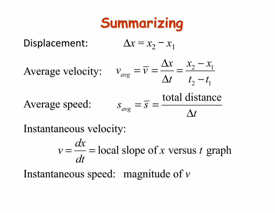
Summarizing

Average velocity: 2 1

2 1avg

x xxv vt t t

−Δ= = =Δ −total distance

avgs st

= =Δ

local slope of versus graphdxv x tdt

= =

Displacement:      Δx = x2 - x1

Instantaneous velocity:

Average speed:

Instantaneous speed: magnitude of v

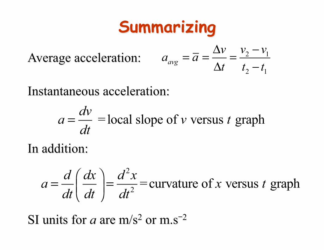
Summarizing

Average acceleration:

Instantaneous acceleration:

In addition:

2 1

2 1avg

v vva at t t

−Δ= = =Δ −

= local slope of versus graphdva v tdt

=

2

2 =curvature of versus graphd dx d xa x tdt dt dt⎛ ⎞= =⎜ ⎟⎝ ⎠

SI units for a are m/s2 or m.s-2

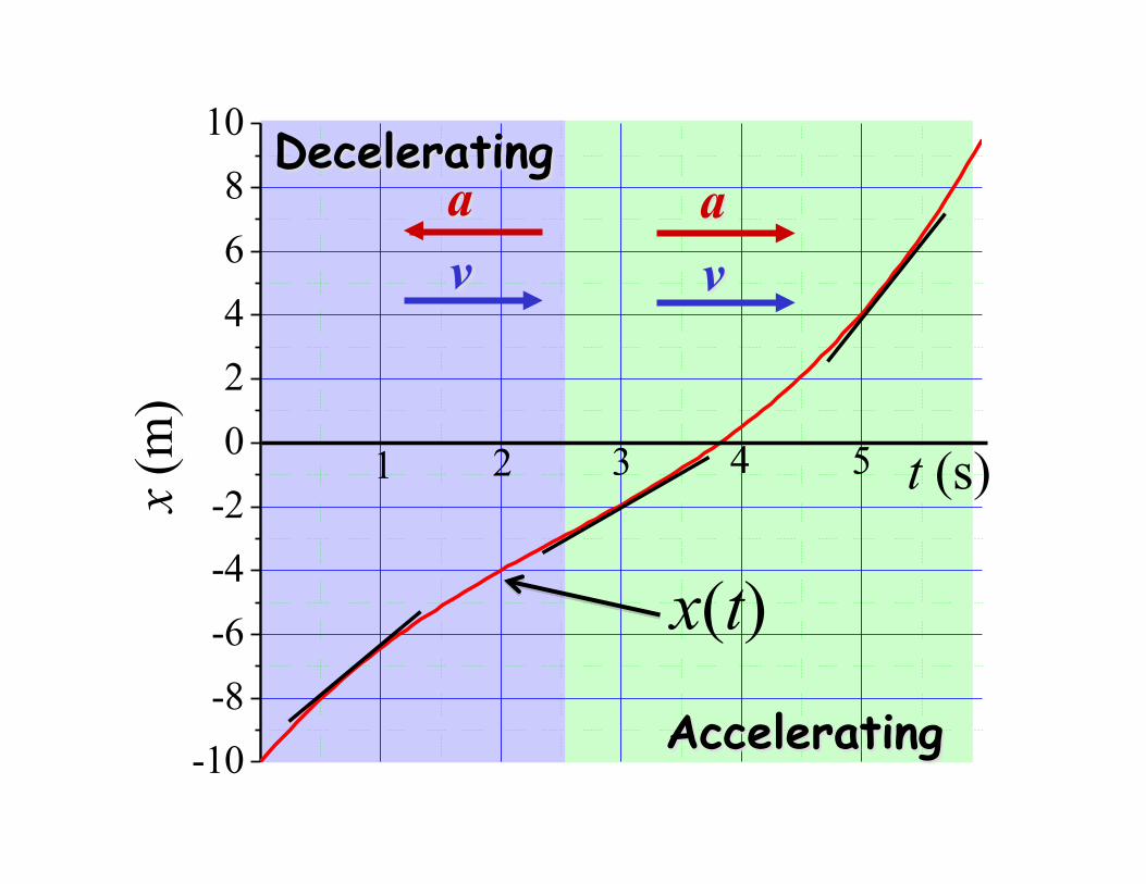
-10-8-6-4-202468

10

t (s)54321x (m

)

Accelerating

a v

Decelerating a v

x(t)

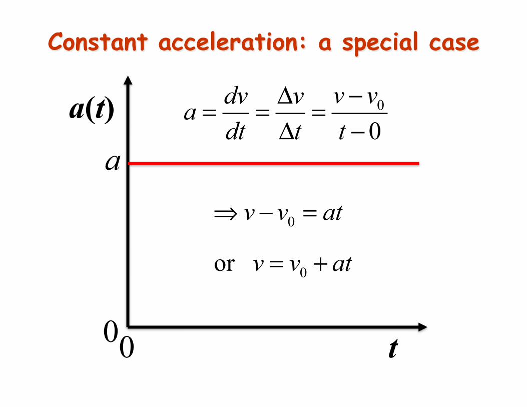
Constant acceleration: a special case

a(t)

t

0

0v vdv va

dt t t−Δ= = =

Δ −a

0

0or

v v at

v v at

⇒ − =

= +

0 0

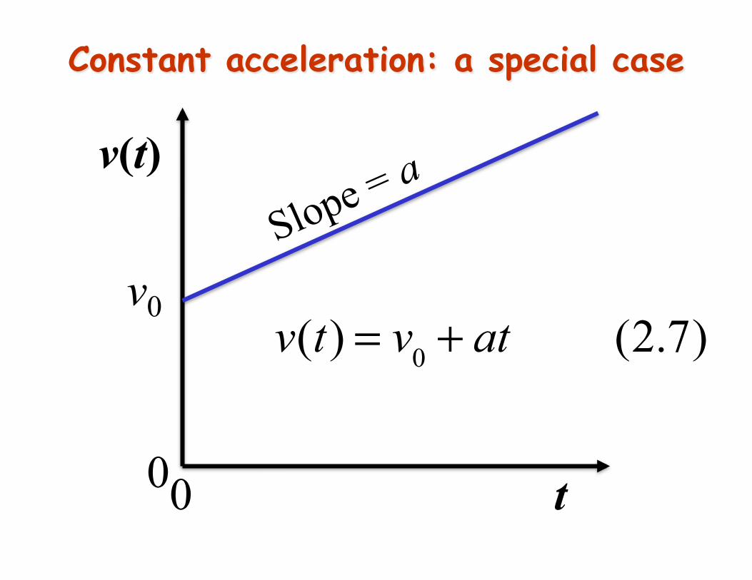
v(t) = v0 + at (2.7)

Constant acceleration: a special case

v(t)

t

v0

0 0

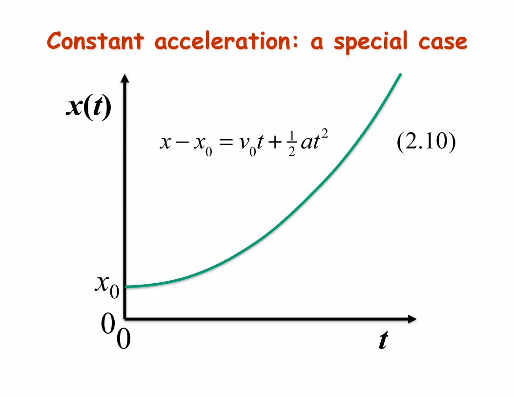
Constant acceleration: a special case

x(t)

t 0 0

x − x0 = v0t +12 at2 (2.10)

x0

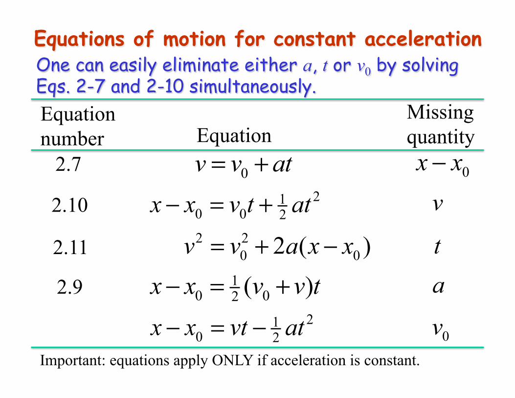
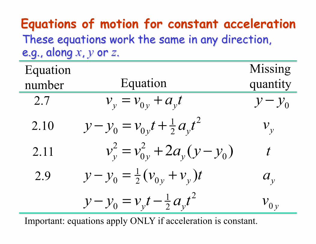
Equations of motion for constant acceleration

210 0 2x x v t at− = +

0v v at= +

2 20 02 ( )v v a x x= + −1

0 02 ( )x x v v t− = +21

0 2x x vt at− = −

0x x−v

ta

0v

Equation Missing quantity

Equation number

2.7

2.10

2.11

2.9

One can easily eliminate either a, t or v0 by solving Eqs. 2-7 and 2-10 simultaneously.

Important: equations apply ONLY if acceleration is constant.

Equations of motion for constant acceleration

210 0 2y yy y v t a t− = +

0y y yv v a t= +

2 20 02 ( )y y yv v a y y= + −1

0 02 ( )y yy y v v t− = +21

0 2y yy y v t a t− = −

0y y−

yv

t

ya

0 yv

Equation Missing quantity

Equation number

2.7

2.10

2.11

2.9

These equations work the same in any direction, e.g., along x, y or z.

Important: equations apply ONLY if acceleration is constant.

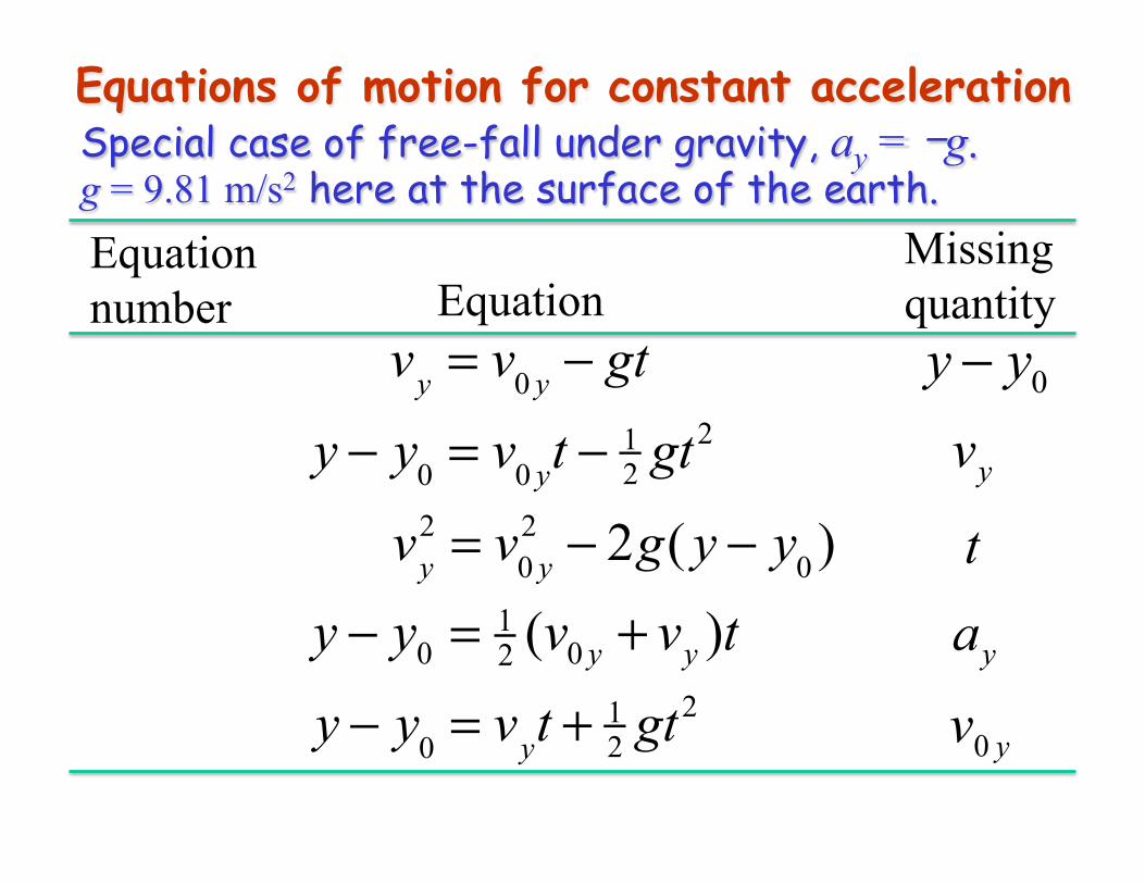
Equations of motion for constant acceleration

y − y0 = v0 yt − 1

2 gt2 vy = v0 y − gt

vy

2 = v0 y2 − 2g( y − y0 )1

0 02 ( )y yy y v v t− = +

y − y0 = vyt + 1

2 gt2

0y y−

yv

t

ya

0 yv

Equation Missing quantity

Equation number

Special case of free-fall under gravity, ay = -g. g = 9.81 m/s2 here at the surface of the earth.

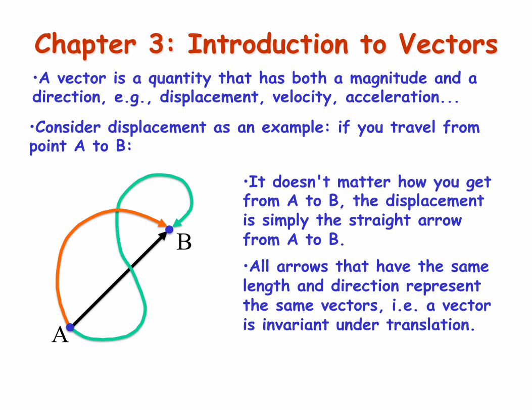
Chapter 3: Introduction to Vectors

• Consider displacement as an example: if you travel from point A to B:

• It doesn't matter how you get from A to B, the displacement is simply the straight arrow from A to B. • All arrows that have the same length and direction represent the same vectors, i.e. a vector is invariant under translation.

• A vector is a quantity that has both a magnitude and a direction, e.g., displacement, velocity, acceleration...

A

B

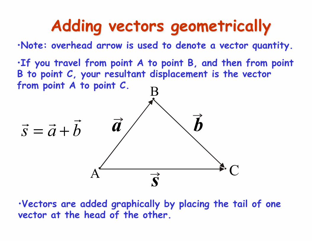
Adding vectors geometrically

• If you travel from point A to point B, and then from point B to point C, your resultant displacement is the vector from point A to point C.

A

B

a

C

b

s

!s = !a +

!b

• Vectors are added graphically by placing the tail of one vector at the head of the other.

• Note: overhead arrow is used to denote a vector quantity.

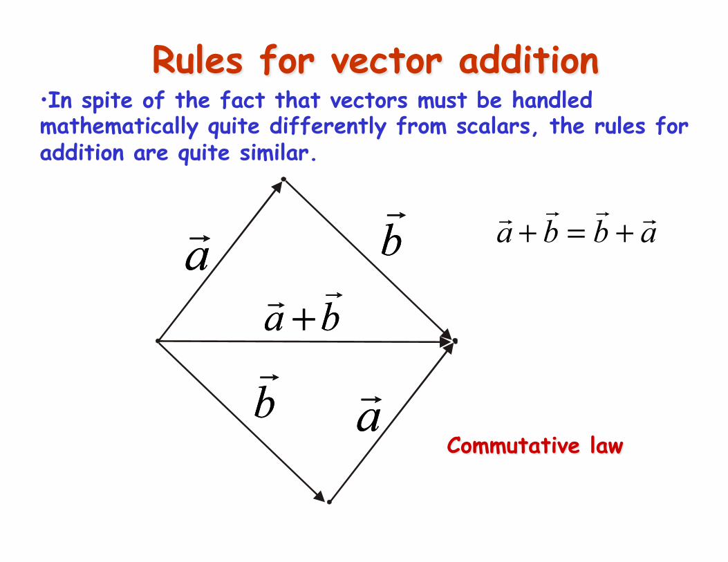
Rules for vector addition • In spite of the fact that vectors must be handled mathematically quite differently from scalars, the rules for addition are quite similar.

a!a b!b

a b+!!a b+

b!b a!a

!a +!b =!b + !a

Commutative law

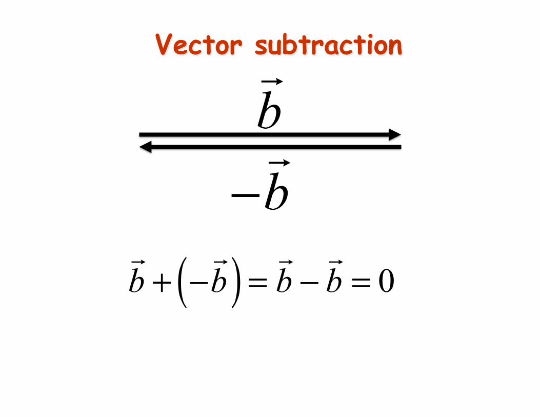
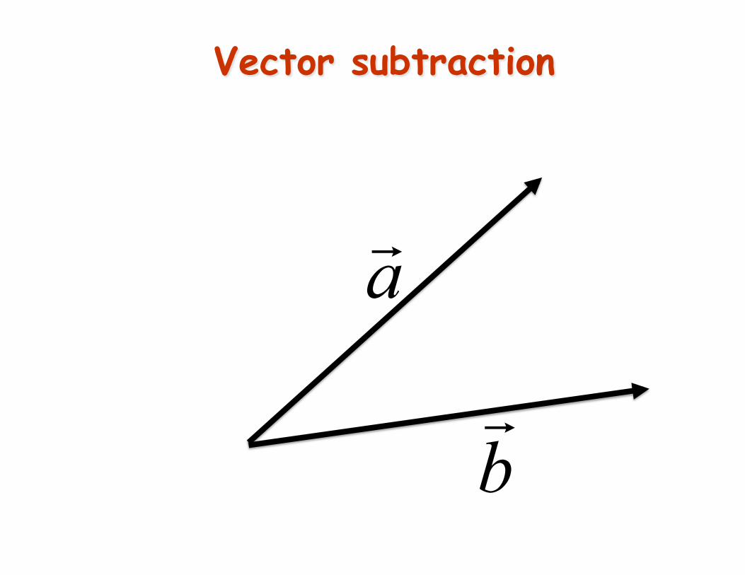
Vector subtraction

!b + −

!b( ) = !b −

!b = 0

−!b !b

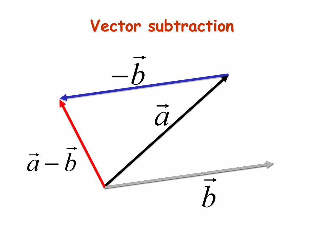
Vector subtraction

!b

!a

−!b

!a −!b

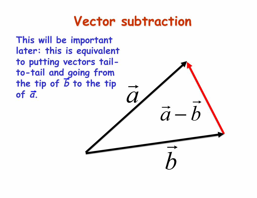
Vector subtraction

!b

!a

!a −!b

This will be important later: this is equivalent to putting vectors tail-to-tail and going from the tip of b to the tip of a.

Vector subtraction

!b

!a

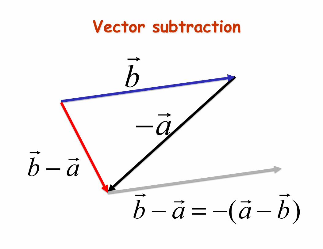
Vector subtraction

−!a

!b

!b − !a

!b − !a = −( !a −

!b)

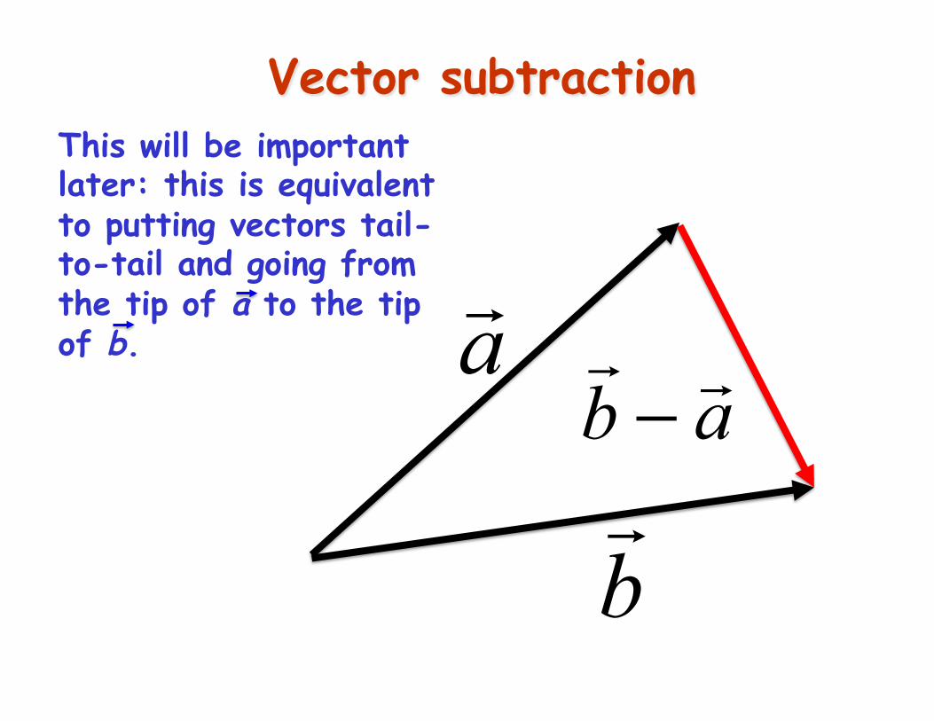
Vector subtraction

!b

!a

!b − !a

This will be important later: this is equivalent to putting vectors tail-to-tail and going from the tip of a to the tip of b.

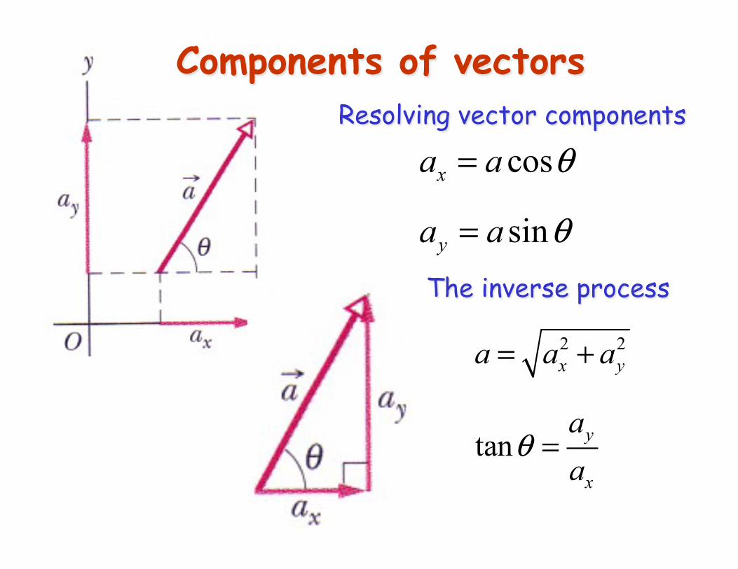
Components of vectors

cos

sin

x

y

a a

a a

θ

θ

=

=

Resolving vector components

The inverse process

2 2

tan

x y

y

x

a a a

aa

θ

= +

=

Unit vectors

i , j and k are unit vectors

They have length equal to unity (1), and point respectively along the x, y and z axes of a right handed Cartesian coordinate system.

x

y

z

!a = axi + ay j

ay j

axi

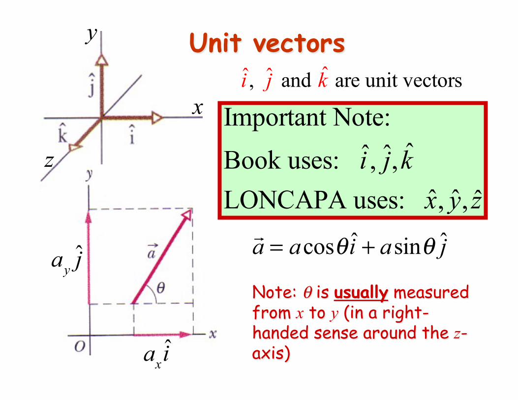
Unit vectors

x

y

z

!a = acosθ i + asinθ j

Note: θ is usually measured from x to y (in a right- handed sense around the z-axis)

ay j

axi

They have length equal to unity (1), and point respectively along the x, y and z axes of a right handed Cartesian coordinate system.

i , j and k are unit vectors

Important Note:Book uses: i , j, kLONCAPA uses: x, y, z

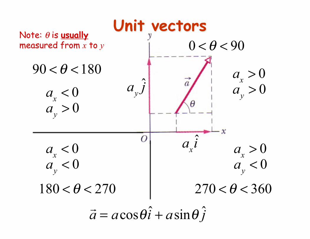
!a = acosθ i + asinθ j

ay j

axi

Unit vectors

90 <θ <180

180 <θ < 270 270 <θ < 360

ax > 0ay < 0

ax < 0ay < 0

ax < 0ay > 0

Note: θ is usually measured from x to y 0 <θ < 90

ax > 0ay > 0

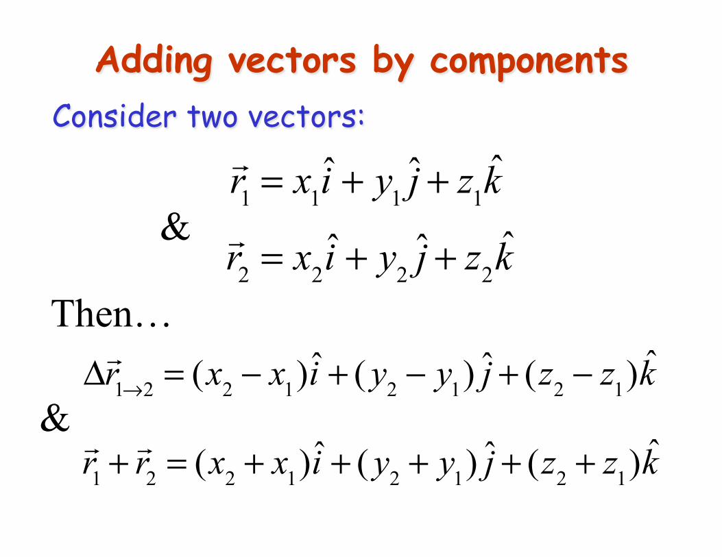
Adding vectors by components

Consider two vectors:

!r2 = x2i + y2 j + z2k

&

Δ!r1→2 = (x2 − x1)i + ( y2 − y1) j + (z2 − z1)k

!r1 +!r2 = (x2 + x1)i + ( y2 + y1) j + (z2 + z1)k

Then…

&

!r1 = x1i + y1 j + z1k

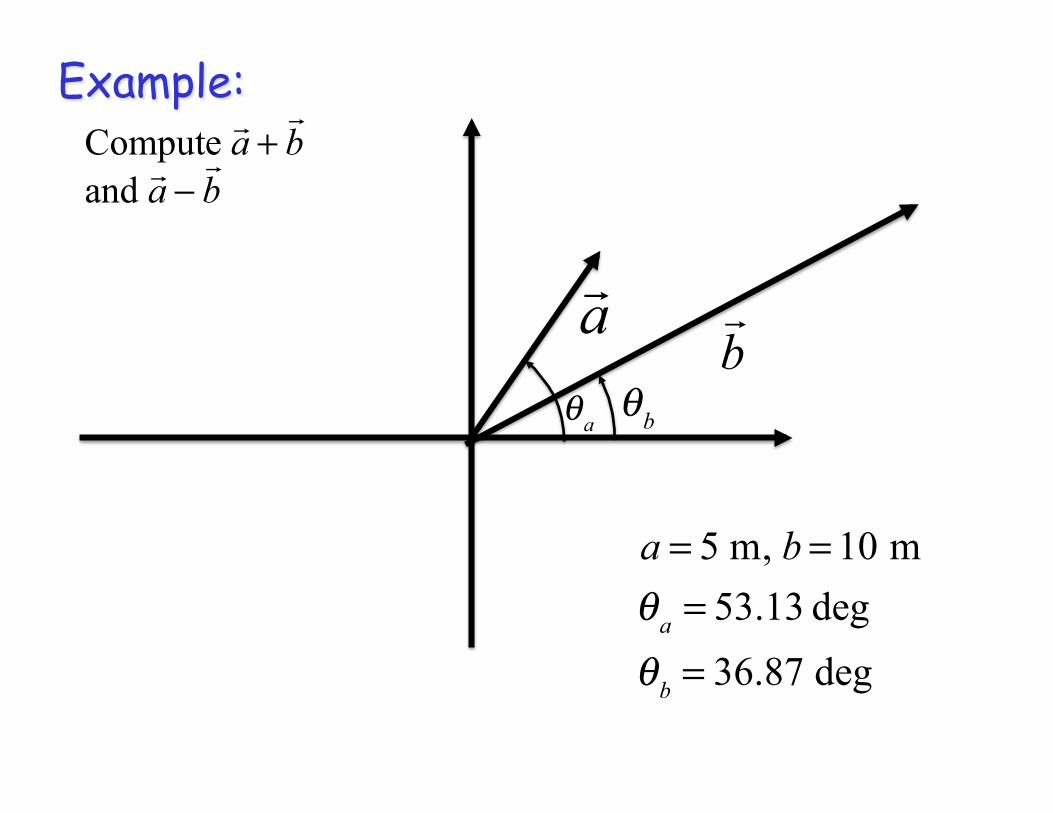
!a

!b

a = 5 m, b = 10 mθa = 53.13 degθb = 36.87 deg

θa θb

Example: Compute

!a +!b

and !a −!b

Appendices

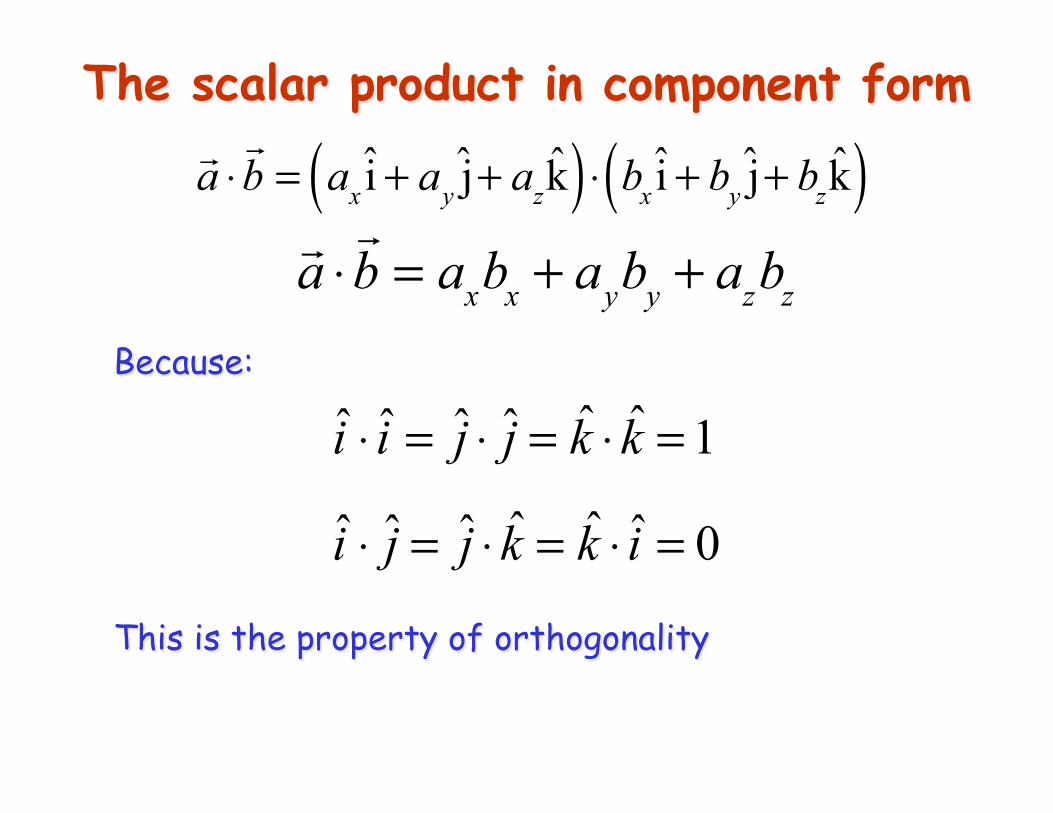
The scalar product in component form

!a ⋅!b = ax i + ay j+ azk( ) ⋅ bx i + by j+ bzk( )

!a ⋅!b = axbx + ayby + azbz

Because:

i ⋅ i = j ⋅ j = k ⋅ k = 1

i ⋅ j = j ⋅ k = k ⋅ i = 0

This is the property of orthogonality

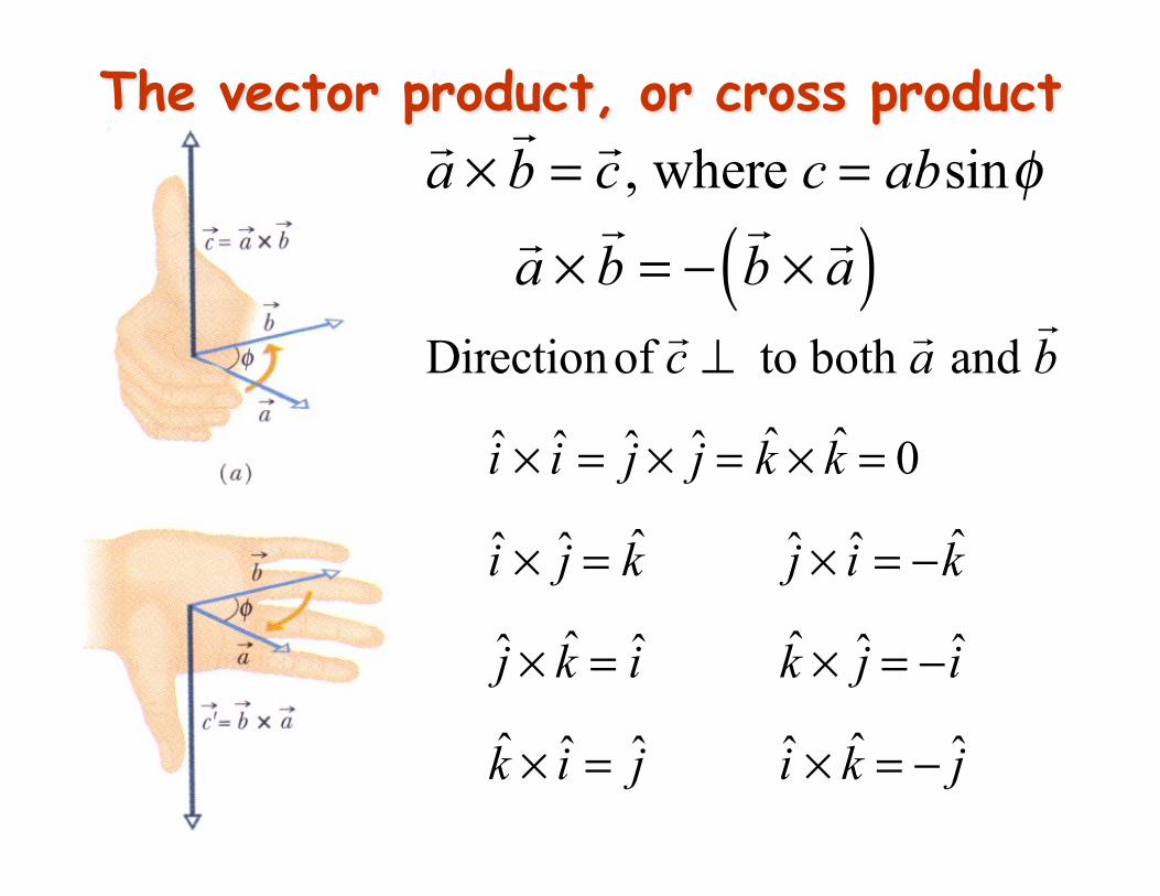
The vector product, or cross product

!a ×!b = !c , where c = absinφ

!a ×!b = −

!b × !a( )

Directionof!c ⊥ to both

!a and !b

i × i = j × j = k × k = 0

i × j = k j × i = − k

j × k = i k × j = − i

k × i = j i × k = − j

i

jk j+ve

i

jk j-ve

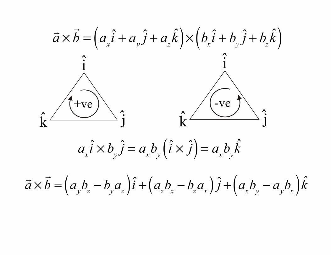
!a ×!b = axi + ay j + azk( )× bxi + by j + bzk( )

axi × by j = axby i × j( ) = axbyk

!a ×!b = aybz − byaz( ) i + azbx − bzax( ) j + axby − aybx( ) k