chapters 21 & 22 modern portfolio theory equilibrium …€¦ · · 2017-05-10modern...

Chapters 21 & 22Modern Portfolio Theory

&Equilibrium Asset Pricing

Chapters 21 & 22

Modern Portfolio Theory

&

Equilibrium Asset Pricing

"MODERN PORTFOLIO THEORY"

(aka "Mean-Variance Portfolio Theory", or “Markowitz Portfolio Theory” – Either way: “MPT” for short)

DEVELOPED IN 1950s (by MARKOWITZ, SHARPE, LINTNER)

(Won Nobel Prize in Economics in 1990.)

WIDELY USED AMONG PROFESSIONAL INVESTORS

FUNDAMENTAL DISCIPLINE OF PORTFOLIO-LEVEL INVESTMENT STRATEGIC DECISION MAKING.

I. REVIEW OF STATISTICS ABOUT PERIODIC TOTAL RETURNS:(Note: these are all “time-series” statistics: measured across time, not across assets within a single point in time.)

"1st Moment" Across Time (measures “central tendency”): “MEAN”, used to measure:

Expected Performance ("ex ante", usually arithmetic mean: used in portf ana.) Achieved Performance ("ex post", usually geometric mean)

"2nd Moments" Across Time (measure characteristics of the deviation around the central tendancy). They include… 1) "STANDARD DEVIATION" (aka "volatility"), which measures:

Square root of variance of returns across time. "Total Risk" (of exposure to asset if investor not diversified)

2) "COVARIANCE", which measures "Co-Movement", aka: "Systematic Risk" (component of total risk which cannot be "diversified away") Covariance with investor’s portfolio measures asset contribution to portfolio total

risk.

3) "CROSS-CORRELATION" (just “correlation” for short). Based on contemporaneous covariance between two assets or asset classes. Measures how two assets "move together":

important for Portfolio Analysis.

4) "AUTOCORRELATION" (or “serial correlation”: Correlation with itself across time), which reflects the nature of the "Informational Efficiency" in the Asset Market; e.g.:

Zero "Efficient" Market (prices quickly reflect full information; returns lack predictability) Like securities markets (approximately).

Positive "Sluggish" (inertia, inefficient) Market (prices only gradually incorporate new info.) Like private real estate markets.

Negative "Noisy" Mkt (excessive s.r. volatility, price "overreactions") Like securities markets (to some extent).

Note: Some review or skimming of Chapter 9 in the text (as well as perhaps the Appendix at the back of Chapter 21) might be helpful. In 11.431 we were primarily dealing with the dollar-weighted multi-period IRR measure of investment return. In 11.432 (apart from Chs.28&29), we will be primarily dealing with periodic returns as the fundamental measure of investment performance.

"Picture" of 1st and 2nd Moments . . .

First Moment is "Trend“. Second Moment is "Deviation" around trend. Food for Thought Question: IF THE TWO LINES ABOVE WERE TWO DIFFERENT ASSETS, WHICH WOULD YOU PREFER TO INVEST IN, OTHER THINGS BEING EQUAL? . . .

The two assets have the same historical geometric mean return but one has a lot more risk. But the two do not have the same arithmetic return. (Which has the higher arithmetic mean?)

Historical statistics, annual periodic total returns: Stocks, Bonds, Real Estate, 1970-2001…

What do these historical 2nd moments (esp. the correlations) “look like”? . . .

1st Moments

2nd Moments

Historical statistics, annual periodic total returns: Stocks, Bonds, Real Estate, 1970-2001…

100%100%PrivPriv. Real Estate. Real Estate

--18.34%18.34%100%100%LTG BondsLTG Bonds

11.83%11.83%36.61%36.61%100%100%S&P500S&P500

Correlations:Correlations:

9.67%9.67%11.95%11.95%16.67%16.67%Std.DeviationStd.Deviation

9.65%9.65%9.75%9.75%13.30%13.30%Mean (Mean (aritharith))

Private Real Private Real EstateEstate

LTG BondsLTG BondsS&P500S&P500

1st Moments

2nd Moments

PORTFOLIO THEORY IS A WAY TO CONSIDER PORTFOLIO THEORY IS A WAY TO CONSIDER BOTHBOTH THE THE 1ST1ST & & 2ND2ND MOMENTS (& INTEGRATE THE TWO) IN INVESTMENT MOMENTS (& INTEGRATE THE TWO) IN INVESTMENT ANALYSIS.ANALYSIS.

What do these historical 2nd moments (esp. the correlations) “look like”? . . .

Source: See book Chapter 7, p.142.

Stocks & bonds (+37% correlation): Each dot is one year's returns.

Stock & Bond Ann. Returns, 1970-2001: +37% Correlation

-20%

-10%

0%

10%

20%

30%

40%

50%

-30% -20% -10% 0% 10% 20% 30% 40% 50%

Stock Returns

Bon

d R

etur

ns

Stocks & real estate (+12% correlation): Each dot is one year's returns.

Real Est. & Stock Ann. Returns, 1970-2001: +12% Correlation

-20%

-15%

-10%

-5%

0%

5%

10%

15%

20%

25%

30%

-30% -20% -10% 0% 10% 20% 30% 40% 50%

Stock Returns

R.E

. Ret

urns

Why do you suppose there has been this negative correlation?

Bonds & real estate (-18% correlation): Each dot is one year's returns.

Real Est. & Bond Ann. Returns, 1970-2001: -18% Correlation

-20%

-10%

0%

10%

20%

30%

40%

50%

-20% -10% 0% 10% 20% 30%

Real Estate Returns

Bon

d R

etur

ns

Why do you suppose there has been this negative correlation?

Hint: The correlation was negative only during the 1970s & 80s. What do you know about inflation during that period of history?

An important mathematical fact about investment risk & return . . .An important mathematical fact about investment risk & return . . .

“Normal”“Normal” risk (volatility) accumulates roughly with the risk (volatility) accumulates roughly with the SQUARE ROOTSQUARE ROOT of time (holding period)of time (holding period)

Projected Value Index Level & +/- 1STD range

0.0

0.5

1.0

1.5

2.0

2.5

3.0

3.5

4.0

4.5

0 3 5 8 9 10

Holding Period (yrs)

Inde

x Le

vel (

1=st

art)

E[V] +1STD -20% Autocorr -1STD -20% Autocorr +1STD 0 Autocorr -1STD 0 Autocorr +1STD +20% Autocorr -1STD +20% Autocorr

2 1 4 7 6

An important mathematical fact about investment risk & return . . .An important mathematical fact about investment risk & return . . .

“Normal”“Normal” risk (volatility) as a risk (volatility) as a proportion of expected returnproportion of expected return diminishesdiminishes with the with the lengthlength of the expected of the expected holding periodholding period..

1STD Value Index as Fraction of Holding Period Expected Simple Return

0.0

0.1

0.2

0.3

0.4

0.5

0.6

0.7

0.8

0.9

1.0

1.1

1 2 3 4 5 9 10

Holding Period (yrs)

Vola

tility

/ Ex

ptdR

etur

n

-20% Autocorr 0% Autocorr +20% Autocorr

8 7 6

The graph is based on an assumed 1st-order autoregressive process in the investment returns, an AR(1) with “rho” parameter value equal to +0.2, -0.2, or zero (random walk), and is based on compounded geometric growth. As a simpler example, working with additive continuously-compounded return (log-differences), with zero autocorrelation (random walk), the volatility increases exactly with the square root of the holding period, while the expected return increases in exact direct linear proportion to the length of the holding period. Thus, the volatility as a proportion of the return decreases with the square root of the holding period.

Thus, as far as “normal” risk is concerned: • The longer your investment holding horizon, the less important risk is to you, i.e.,• You can afford to be more “aggressive” in your investments (less “risk averse”), • Other things being equal (in particular, holding your fundamental risk preferences the same).

What is “normal” risk? . . .

Thus, as far as “normal” risk is concerned: • The longer your investment holding horizon, the less important risk is to you, i.e., • You can afford to be more “aggressive” in your investments (less “risk averse”), • Other things being equal (in particular, holding your fundamental risk preferences the same).

What is “normal” risk? . . .

“Normal”“Normal” risk is the regular, ordinary type of risk that always exists, risk is the regular, ordinary type of risk that always exists, every every day, in the investment world, due to the fact that the future isday, in the investment world, due to the fact that the future is uncertain uncertain and and “news”“news” is continuously arriving about the unfolding future.is continuously arriving about the unfolding future.

“Normal”“Normal” risk is the dominant type of risk in modern, developed economierisk is the dominant type of risk in modern, developed economies s such as the U.S.such as the U.S.

“Normal”“Normal” risk is the subject of MPT, and is well modeled statistically brisk is the subject of MPT, and is well modeled statistically by the y the Normal probability distribution, by continuous time, and by periNormal probability distribution, by continuous time, and by periodic odic return timereturn time--series 2series 2ndnd--moment statistics such as variance, volatility moment statistics such as variance, volatility ((std.devstd.dev.), covariance, and .), covariance, and “beta”“beta”..

You may ask: “What is non-normal risk”? Non-normal risk is the risk posed by relatively rare, exceptional, “major events” (typically of a negative or “bad news” nature, that is, on the “downside” of the future return probability). Such events typically affect many or even all asset classes simultaneously. They occur at discrete, random points in time (unpredictably, of course, or they would not be “risk”). From a mathematical perspective, such discrete major events cause the normal probability distribution to not be a perfect model of the risk in investment returns. Non-normal risk is not rigorously addressed by classical MPT, and it may be at least partly responsible for why “beta” and the CAPM do not work perfectly to predict the cross section of expected returns in the stock market.

II. WHAT IS PORTFOLIO THEORY?...

SUPPOSE WE DRAW A 2-DIMENSIONAL SPACE WITH RISK (2ND-MOMENT) ON HORIZONTAL AXIS AND EXPECTED RETURN (1ST MOMENT) ON VERTICAL AXIS.

A RISK-AVERSE INVESTOR MIGHT HAVE A UTILITY (PREFERENCE) SURFACE INDICATED BY CONTOUR LINES LIKE THESE (investor is indifferent along a given contour line):

RISK

RETURN

THE CONTOUR LINES ARE STEEPLY RISING AS THE RISK-AVERSE INVESTOR WANTS MUCH MORE RETURN TO COMPENSATE FOR A LITTLE MORE RISK.

II. WHAT IS PORTFOLIO THEORY?...

SUPPOSE WE DRAW A 2-DIMENSIONAL SPACE WITH RISK (2ND-MOMENT) ON HORIZONTAL AXIS AND EXPECTED RETURN (1ST MOMENT) ON VERTICAL AXIS.

A RISK-AVERSE INVESTOR MIGHT HAVE A UTILITY (PREFERENCE) SURFACE INDICATED BY CONTOUR LINES LIKE THESE (investor is indifferent along a given contour line):

RETURNP

Q

RISK

THE CONTOUR LINES ARE STEEPLY RISING AS THE RISK-AVERSE INVESTOR WANTS MUCH MORE RETURN TO COMPENSATE FOR A LITTLE MORE RISK.

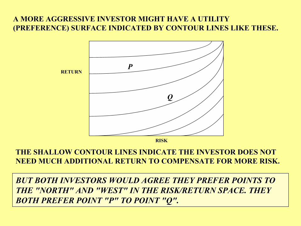
A MORE AGGRESSIVE INVESTOR MIGHT HAVE A UTILITY (PREFERENCE) SURFACE INDICATED BY CONTOUR LINES LIKE THESE.

RISK

RETURN

THE SHALLOW CONTOUR LINES INDICATE THE INVESTOR DOES NOT NEED MUCH ADDITIONAL RETURN TO COMPENSATE FOR MORE RISK.

A MORE AGGRESSIVE INVESTOR MIGHT HAVE A UTILITY (PREFERENCE) SURFACE INDICATED BY CONTOUR LINES LIKE THESE.

RETURN

RISK

THE SHALLOW CONTOUR LINES INDICATE THE INVESTOR DOES NOT NEED MUCH ADDITIONAL RETURN TO COMPENSATE FOR MORE RISK.

P

Q

BUT BOTH INVESTORS WOULD AGREE THEY PREFER POINTS TO BUT BOTH INVESTORS WOULD AGREE THEY PREFER POINTS TO THE "NORTH" AND "WEST" IN THE RISK/RETURN SPACE. THEY THE "NORTH" AND "WEST" IN THE RISK/RETURN SPACE. THEY BOTH PREFER POINT "P" TO POINT "Q".BOTH PREFER POINT "P" TO POINT "Q".

FOR ANY TWO PORTFOLIOS "P" AND "Q" SUCH THAT:EXPECTED RETURN "P" ≥ EXPECTED RETURN "Q"

AND (SIMULTANEOUSLY): RISK "P" ≤ RISK "Q"IT IS SAID THAT: “Q” IS DOMINATED BY “P”.

THIS IS INDEPENDENT OF RISK PREFERENCES. BOTH CONSERVATIVE AND AGGRESSIVE INVESTORS WOULD

AGREE ABOUT THIS.

IN ESSENCE, PORTFOLIO THEORY IS ABOUT HOW TO AVOID INVESTING IN DOMINATED PORTFOLIOS.

RISK

RETURN

PORTFOLIO THEORY TRIES TO MOVE INVESTORSFROM POINTS LIKE "Q" TO POINTS LIKE "P".

FOR ANY TWO PORTFOLIOS "P" AND "Q" SUCH THAT: EXPECTED RETURN "P" ≥ EXPECTED RETURN "Q"

AND (SIMULTANEOUSLY): RISK "P" ≤ RISK "Q" IT IS SAID THAT: “Q” IS DOMINATED BY “P”.

THIS IS INDEPENDENT OF RISK PREFERENCES. BOTH CONSERVATIVE AND AGGRESSIVE INVESTORS WOULD

AGREE ABOUT THIS.

IN ESSENCE, PORTFOLIO THEORY IS ABOUT HOW TO AVOID INVESTING IN DOMINATED PORTFOLIOS.

RETURN P

Q DOMINATED

BY "Q"

DOMINATES "Q"

DOMINATES "Q"

RISK

PORTFOLIO THEORY TRIES TO MOVE INVESTORSFROM POINTS LIKE "Q" TO POINTS LIKE "P".

Got through here 1st class

III. PORTFOLIO THEORY AND DIVERSIFICATION...

"PORTFOLIOS" ARE "COMBINATIONS OF ASSETS".

PORTFOLIO THEORY FOR (or from) YOUR GRANDMOTHER:

“DON’T PUT ALL YOUR EGGS IN ONE BASKET!”

WHAT MORE THAN THIS CAN WE SAY? . . .

(e.g., How many “eggs” should we put in which “baskets”.)

In other words, GIVEN YOUR OVERALL INVESTABLE WEALTH, PORTFOLIO THEORY TELLS YOU HOW MUCH YOU SHOULD INVEST IN DIFFERENT TYPES OF ASSETS. FOR EXAMPLE:

WHAT % SHOULD YOU PUT IN REAL ESTATE? WHAT % SHOULD YOU PUT IN STOCKS?

TO BEGIN TO RIGOROUSLY ANSWER THIS QUESTION, CONSIDER...

AT THE HEART OF PORTFOLIO THEORY ARE TWO BASIC AT THE HEART OF PORTFOLIO THEORY ARE TWO BASIC MATHEMATICAL MATHEMATICAL FACTSFACTS::

1) PORTFOLIO RETURN IS A LINEAR FUNCTION OF THE ASSET 1) PORTFOLIO RETURN IS A LINEAR FUNCTION OF THE ASSET WEIGHTS:WEIGHTS:

IN PARTICULAR, THE PORTFOLIO EXPECTED RETURN IS A IN PARTICULAR, THE PORTFOLIO EXPECTED RETURN IS A WEIGHTED AVERAGEWEIGHTED AVERAGE OF THE EXPECTED RETURNS TO THE OF THE EXPECTED RETURNS TO THE INDIVIDUAL ASSETS. E.G., WITH TWO ASSETS ("i" & "j"):INDIVIDUAL ASSETS. E.G., WITH TWO ASSETS ("i" & "j"):

rrpp = = ωωrrii + (1+ (1--ωω))rrjj

WHERE WHERE ωωii IS THE SHARE OF PORTFOLIO TOTAL VALUE INVESTED IS THE SHARE OF PORTFOLIO TOTAL VALUE INVESTED IN ASSET i.IN ASSET i.

e.g., If Asset A has E[rA]=5% and Asset B has E[rB]=10%, then a 50/50 Portfolio (50% A + 50% B) will have E[rP]=7.5%.

rw=r nn

N

1=nP ∑

2) PORTFOLIO VOLATILITY IS A NON2) PORTFOLIO VOLATILITY IS A NON--LINEAR FUNCTION OF THE LINEAR FUNCTION OF THE ASSET WEIGHTS:ASSET WEIGHTS:

SUCH THAT THE PORTFOLIO VOLATILITY IS SUCH THAT THE PORTFOLIO VOLATILITY IS LESS THANLESS THAN A A WEIGHTED AVERAGE OF THE VOLATILITIES OF THE WEIGHTED AVERAGE OF THE VOLATILITIES OF THE INDIVIDUAL ASSETS. E.G., WITH TWO ASSETS:INDIVIDUAL ASSETS. E.G., WITH TWO ASSETS:

This is the beauty of Diversification. It is at the core of Portfolio Theory. It is perhaps the only place in economics where you get a “free lunch”: In this case, less risk without necessarily reducing your expected return!

e.g., If Asset A has StdDev[rA]=5% and Asset B has StdDev[rB]=10%, then a 50/50 Portfolio (50% A + 50% B) will have StdDev[rP] < 7.5% (conceivably even < 5%).

THE 2THE 2NDND FACT:FACT:

ssPP = = √√[ [ ωω²²(s(sii))²² + (1+ (1--ωω))²²(s(sjj))²² + 2+ 2ωω(1(1--ωω)s)siissjjCCij ij ] ]

≤≤ ωωssii + (1+ (1--ωω)s)sjj

WHERE WHERE ssii IS THE RISK (MEASURED BY STD.DEV.) OF ASSET i.IS THE RISK (MEASURED BY STD.DEV.) OF ASSET i.

∑∑= =

=N

I

N

JijjiP COVwwVAR

1 1

For example, a portfolio of 50% bonds & 50% real estate would haFor example, a portfolio of 50% bonds & 50% real estate would have had less ve had less volatility than either asset class alone during 1970volatility than either asset class alone during 1970--2001, but a very similar return:2001, but a very similar return:

Annual Historical Returns: Bond Portf, R.E. Portf, Half&Half Portf

-30%

-20%

-10%

0%

10%

20%

30%

40%

50%19

70

1972

1974

1976

1978

1980

1982

1984

1986

1988

1990

1992

1994

1996

1998

2000

Bonds R.Estate HalfBnRE

7.0%7.0%9.7%9.7%12.0%12.0%Std.DevStd.Dev..9.7%9.7%9.7%9.7%9.7%9.7%MeanMean

Half&HalfHalf&HalfR.EstateR.EstateBondsBondsReturns:Returns:

Data Source: See textbook Ch.7, p.142.

This This ““Diversification EffectDiversification Effect”” is greater, the lower is the correlation among the is greater, the lower is the correlation among the assets in the portfolio.assets in the portfolio.

NUMERICAL EXAMPLE . . . SUPPOSE REAL ESTATE HAS: SUPPOSE STOCKS HAVE: EXPECTED RETURN = 8% EXPECTED RETURN = 12% RISK (STD.DEV) = 10% RISK (STD.DEV) = 15% THEN A PORTFOLIO WITH ω SHARE IN REAL ESTATE & (1-ω) SHARE IN STOCKS WILL RESULT IN THESE RISK/RETURN COMBINATIONS, DEPENDING ON THE CORRELATION BETWEEN THE REAL ESTATE AND STOCK RETURNS:

C = 100% C = 25% C = 0% C = -50% ω rP sP rP sP rP sP rP sP 0% 12.0% 15.0% 12.0% 15.0% 12.0% 15.0% 12.0% 15.0%25% 11.0% 13.8% 11.0% 12.1% 11.0% 11.5% 11.0% 10.2%50% 10.0% 12.5% 10.0% 10.0% 10.0% 9.0% 10.0% 6.6%75% 9.0% 11.3% 9.0% 9.2% 9.0% 8.4% 9.0% 6.5%100% 8.0% 10.0% 8.0% 10.0% 8.0% 10.0% 8.0% 10.0%where: C = Correlation Coefficient between Stocks & Real Estate. (This table was simply computed using the formulas noted previously.)

Correlation = 100%

8%

9%

10%

11%

12%

9% 10% 11% 12% 13% 14% 15%Portf Risk (STD)

Port

f Exp

td R

etur

n3/4 RE

1/2 RE

1/4 RE

Correlation = 25%

8%

9%

10%

11%

12%

9% 10% 11% 12% 13% 14% 15%Portf Risk (STD)

Port

f Exp

td R

etur

n

1/4 RE

1/2 RE

3/4 RE

This This ““Diversification EffectDiversification Effect”” is greater, the lower is the correlation among the is greater, the lower is the correlation among the assets in the portfolio.assets in the portfolio.

IN ESSENCE,IN ESSENCE,

PORTFOLIO THEORY PORTFOLIO THEORY ASSUMESASSUMES::

YOUR YOUR OBJECTIVEOBJECTIVE FOR YOUR FOR YOUR OVERALL WEALTHOVERALL WEALTHPORTFOLIO IS:PORTFOLIO IS:

MAXIMIZE EXPECTED FUTURE RETURNMAXIMIZE EXPECTED FUTURE RETURN

MINIMIZE RISK IN THE FUTURE RETURNMINIMIZE RISK IN THE FUTURE RETURN

GIVEN THIS BASIC ASSUMPTION, AND THE EFFECT OF GIVEN THIS BASIC ASSUMPTION, AND THE EFFECT OF DIVERSIFICATION, WE ARRIVE AT THE FIRST MAJOR DIVERSIFICATION, WE ARRIVE AT THE FIRST MAJOR RESULT OF PORTFOLIO THEORY. . .RESULT OF PORTFOLIO THEORY. . .

With what we just saw about the nature of diversification in mind, let’s now step back to the overall portfolio strategy question that motivates our analysis. Let’s go back to the question: what is the objective of the investor?... (Remember I said that portfolio theory is a way to integrate the first and second moments of investment returns statistics into the analysis)

To the investor, the risk that matters in an investment is that investment's contribution to the risk in the investor's overall portfolio, not the risk in the investment by itself. This means that covariance(correlation and variance) may be as important as (or more important than) variance (or volatility) in the investment alone. (e.g., if the investor's portfolio is primarily in stocks & bonds, and real estate has a low correlation with stocks & bonds, then the volatility in real estate may not matter much to the investor, because it will not contribute much to the volatility in the investor's portfolio. Indeed, it may allow a reduction in the portfolio’s risk.)

THIS IS A MAJOR SIGNPOST ON THE WAY TO FIGURING OUT THIS IS A MAJOR SIGNPOST ON THE WAY TO FIGURING OUT "HOW MANY EGGS" WE SHOULD PUT IN WHICH "BASKETS"."HOW MANY EGGS" WE SHOULD PUT IN WHICH "BASKETS".

IV. QUANTIFYING OPTIMAL PORTFOLIOS: STEP 1: FINDING THE "EFFICIENT FRONTIER". . . SUPPOSE WE HAVE THE FOLLOWING RISK & RETURN EXPECTATIONS (INCUDING CORRELATIONS):

Stocks Bonds REMean 12.00% 7.00% 8.00%STD 15.00% 8.00% 10.00%CorrStocks 100.00% 40.00% 25.00%Bonds 100.00% 0.00%RE 100.00%

INVESTING IN ANY ONE OF THE THREE ASSET CLASSES WITHOUT DIVERSIFICATION ALLOWS THE INVESTOR TO ACHIEVE ONLY ONE OF THREE POSSIBLE RISK/RETURN POINTS…

The two steps are going to be: (1) Identifying the “efficient frontier”, and then (ii) Ascertaining where (which portfolio) the investor should prefer on that frontier. Note: The risk/return expectations employed in this example are not exactly equal to the historical risk/return performances of the three asset classes (see earlier statistics). But what matters for making investment decisions is ex ante expectations, as of the present looking forward into the future. Historical statistics provide relevant information, but not the whole story, in making the kind of subjective, informed judgments (estimates) that decision-makers must make.

INVESTING IN ANY ONE OF THE THREE ASSET CLASSES WITHOUT INVESTING IN ANY ONE OF THE THREE ASSET CLASSES WITHOUT DIVERSIFICATION ALLOWS THE INVESTOR TO ACHIEVE ONLY ONE OF DIVERSIFICATION ALLOWS THE INVESTOR TO ACHIEVE ONLY ONE OF THE THREE POSSIBLE RISK/RETURN POINTS DEPICTED IN THE GRAPH THE THREE POSSIBLE RISK/RETURN POINTS DEPICTED IN THE GRAPH BELOWBELOW……

3 Assets: Stocks, Bonds, RE, No Diversification

7%

9%

11%

6% 8% 10% 12% 14% 16%

Risk (Std.Dev)

E(r)

Stocks Bonds Real Ests

Bonds

Real Est

Stocks

IN A RISK/RETURN CHART LIKE THIS, ONE WANTS TO BE ABLE TO GET ASMANY RISK/RETURN COMBINATIONS AS POSSIBLE, AS FAR TO THE “NORTH” AND “WEST” AS POSSIBLE.

ALLOWING PAIRWISE COMBINATIONS (AS WITH OUR PREVIOUS STOCKS ALLOWING PAIRWISE COMBINATIONS (AS WITH OUR PREVIOUS STOCKS & REAL ESTATE EXAMPLE), INCREASES THE RISK/RETURN & REAL ESTATE EXAMPLE), INCREASES THE RISK/RETURN POSSIBILITIES TO THESEPOSSIBILITIES TO THESE……

3 Assets: Stocks, Bonds, RE, with pairwise combinations

7%

9%

11%

6% 8% 10% 12% 14% 16%

Risk (Std.Dev)

E(r)

RE&Stocks St&Bonds RE&Bonds

Bonds

Real Est

Stocks

FINALLY, IF WE ALLOW UNLIMITED DIVERSIFICATION AMONG ALL THREE FINALLY, IF WE ALLOW UNLIMITED DIVERSIFICATION AMONG ALL THREE ASSET CLASSES, WE ENABLE AN INFINITE NUMBER OF COMBINATIONS, ASSET CLASSES, WE ENABLE AN INFINITE NUMBER OF COMBINATIONS, THE THE ““BESTBEST”” (I.E., MOST (I.E., MOST ““NORTHNORTH”” AND AND ““WESTWEST””) OF WHICH ARE SHOWN ) OF WHICH ARE SHOWN BY THE OUTSIDE (ENVELOPING) CURVE.BY THE OUTSIDE (ENVELOPING) CURVE.

3 Assets with Diversification: The Efficient Frontier

7%

9%

11%

6% 8% 10% 12% 14% 16%

Risk (Std.Dev)

E(r)

Effic.Frontier RE&Stocks St&Bonds RE&Bonds

THIS IS THE “EFFICIENT FRONTIER” IN THIS CASE (OF THREE ASSET CLASSES).

IN PORTFOLIO THEORY THE IN PORTFOLIO THEORY THE ““EFFICIENT FRONTIEREFFICIENT FRONTIER””CONSISTS OF ALL ASSET COMBINATIONS CONSISTS OF ALL ASSET COMBINATIONS (PORTFOLIOS) WHICH MAXIMIZE RETURN AND (PORTFOLIOS) WHICH MAXIMIZE RETURN AND MINIMIZE RISK. MINIMIZE RISK. THE EFFICIENT FRONTIER IS AS FAR THE EFFICIENT FRONTIER IS AS FAR ““NORTHNORTH”” AND AND ““WESTWEST”” AS YOU CAN POSSIBLY GET IN THE AS YOU CAN POSSIBLY GET IN THE RISK/RETURN GRAPH.RISK/RETURN GRAPH.

(Terminology note: This is a different definition of "efficiency(Terminology note: This is a different definition of "efficiency" " than the concept of informational efficiency applied to asset than the concept of informational efficiency applied to asset markets and asset prices.)markets and asset prices.)

A PORTFOLIO IS SAID TO BE A PORTFOLIO IS SAID TO BE “EFFICIENT”“EFFICIENT” (i.e., (i.e., represents one point on the efficient frontier) IF IT HAS THE represents one point on the efficient frontier) IF IT HAS THE MINIMUM POSSIBLE VOLATILITY FOR A GIVEN MINIMUM POSSIBLE VOLATILITY FOR A GIVEN EXPECTED RETURN, AND/OR THE MAXIMUM EXPECTED RETURN, AND/OR THE MAXIMUM EXPECTED RETURN FOR A GIVEN LEVEL OF EXPECTED RETURN FOR A GIVEN LEVEL OF VOLATILITY.VOLATILITY.

SUMMARY UP TO HERE:SUMMARY UP TO HERE:

DIVERSIFICATION AMONG RISKY ASSETS ALLOWS:DIVERSIFICATION AMONG RISKY ASSETS ALLOWS:

GREATER EXPECTED RETURN TO BE OBTAINEDGREATER EXPECTED RETURN TO BE OBTAINED

FOR ANY GIVEN RISK EXPOSURE, &/OR;FOR ANY GIVEN RISK EXPOSURE, &/OR;

LESS RISK TO BE INCURREDLESS RISK TO BE INCURRED

FOR ANY GIVEN EXPECTED RETURN TARGET.FOR ANY GIVEN EXPECTED RETURN TARGET.

(This is called getting on the "efficient frontier".)(This is called getting on the "efficient frontier".)

PORTFOLIO THEORY ALLOWS US TO:PORTFOLIO THEORY ALLOWS US TO:

QUANTIFYQUANTIFY THIS EFFECT OF DIVERSIFICATIONTHIS EFFECT OF DIVERSIFICATION

IDENTIFY THE "IDENTIFY THE "OPTIMALOPTIMAL" (BEST) MIXTURE OF RISKY " (BEST) MIXTURE OF RISKY ASSETSASSETS

MATHEMATICALLY, THIS IS A "CONSTRAINED MATHEMATICALLY, THIS IS A "CONSTRAINED OPTIMIZATION" PROBLEMOPTIMIZATION" PROBLEM

==> Algebraic solution using calculus==> Algebraic solution using calculus

==> Numerical solution using computer and ==> Numerical solution using computer and "quadratic programming". Spreadsheets such as Excel "quadratic programming". Spreadsheets such as Excel include "Solvers" that can find optimal portfolios this include "Solvers" that can find optimal portfolios this way.way.

STEP 2) PICK A RETURN TARGET FOR YOUR OVERALL WEALTH THAT REFLECTS YOUR RISK PREFERENCES...

E.G., ARE YOU HERE (9%)?...E.G., ARE YOU HERE (9%)?...

Optimal portfolio (P) for a conservative investor: Target=9%

7%

8%

9%

10%

11%

12%

6% 8% 10% 12% 14% 16%

Risk (Std.Dev)

E(r)

P = 33%St, 31%Bd, 36%RE

maxrisk/returnindifferencecurve

OR ARE YOU HERE (11%)?...OR ARE YOU HERE (11%)?...

Optimal portfolio (P) for an aggressive investor: Target=11%

7%

8%

9%

10%

11%

12%

6% 8% 10% 12% 14% 16%

Risk (Std.Dev)

E(r)

P= 75%St, 0%Bd, 25%RE

max risk/return indifference curve

How to determine the investor’s risk preferences (target risk and return) is not an exact science. There are some exercises that are often employed (e.g., asking the investor to choose betw various combinations of stocks and bonds, or between various risk/return simulated distributions, or to specify maximum acceptable probability of a given degree of specified loss, etc.,etc.). The final decision ends up usually being both intuitive and “political”, especially for decision-making entities that are “organizations” (e.g., institutions, firms, that is, collectivities of multiple individuals) as opposed to single wealthy individuals. Note that, from a “scientific” perspective, there is no rigorous way to quantitatively aggregate across individuals’ utility functions (“Arrow’s Impossibility Theorem” of welfare economics).

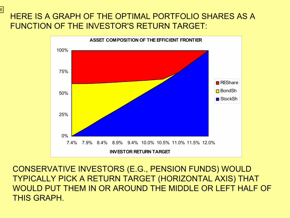
HERE IS A GRAPH OF THE OPTIMAL PORTFOLIO SHARES AS A FUNCTION OF THE INVESTOR'S RETURN TARGET:

ASSET COMPOSITION OF THE EFFICIENT FRONTIER

0%

25%

50%

75%

100%

7.4% 7.9% 8.4% 8.9% 9.4% 10.0% 10.5% 11.0% 11.5% 12.0%

INVESTOR RETURN TARGET

REShare

BondSh

StockSh

CONSERVATIVE INVESTORS (E.G., PENSION FUNDS) WOULD TYPICALLY PICK A RETURN TARGET (HORIZONTAL AXIS) THAT WOULD PUT THEM IN OR AROUND THE MIDDLE OR LEFT HALF OF THIS GRAPH.

THIS LEADS TO SOME IMPORTANT (AND FAMOUS) POLICY IMPLICATIONS...

V. GENERAL QUALITATIVE RESULTS OF PORTFOLIO THEORY

1) THE OPTIMAL REAL ESTATE SHARE DEPENDS ON HOW CONSERVATIVE OR AGGRESSIVE IS THE INVESTOR;

2) FOR MOST OF THE RANGE OF RETURN TARGETS, REAL ESTATE IS A SIGNIFICANT SHARE. (COMPARE THESE SHARES TO THE AVERAGE PENSION FUND REAL ESTATE ALLOCATION WHICH IS LESS THAN 5%. THIS IS WHY PORTFOLIO THEORY HAS BEEN USED TO TRY TO GET INCREASED PF ALLOCATION TO REAL ESTATE.)

3) THE ROBUSTNESS OF REAL ESTATE'S INVESTMENT APPEAL IS DUE TO ITS LOW CORRELATION WITH BOTH STOCKS & BONDS, THAT IS, WITH ALL OF THE REST OF THE PORTFOLIO. (NOTE IN PARTICULAR THAT OUR INPUT ASSUMPTIONS IN THE ABOVE EXAMPLE NUMBERS DID NOT INCLUDE A PARTICULARLY HIGH RETURN OR PARTICULARLY LOW VOLATILITY FOR THE REAL ESTATE ASSET CLASS. THUS, THE LARGE REAL ESTATE SHARE IN THE OPTIMAL PORTFOLIO MUST NOT BE DUE TO SUCH ASSUMPTIONS.)

VI. Technical aside…

Opening the “black box”: Nuts & bolts of Mean-Variance Portfolio Theory...

THE THREE STEPS IN CALCULATING EFFICIENT PORTFOLIOS:

A) INPUT INVESTOR EXPECTATIONS:

We need the following input information:

1) Mean (i.e., expected) return for each asset;

2) Volatility (i.e., Standard Deviation of Returns across time) for each asset class;

3) Correlation coefficients between each pair of asset classes.

B) ENTER COMPUTATION FORMULAS INTO THE SPREADSHEET:We need the following mathematical formulas and tools . . .

(These are the same formulas we have previously noted.)1) The formula for the return of a portfolio (& for portfolio expected return as a function of constituent assets expected returns):

rw=r nn

N

1=nP ∑

(The weighted avg of the constituent returns, where the weights, wn, sum to 1.)

2) The formula for the variance (volatility squared) of a portfolio:

∑∑= =

=N

I

N

JijjiP COVwwVAR

1 1where: VARP = PORTFOLIO RETURN VARIANCE OF A PORTFOLIO WITH N ASSETS, wJ = WEIGHT (PORTFOLIO VALUE SHARE) IN ASSET “j”,COVij = COVARIANCE BETWEEN THE RETURNS TO ASSETS “i” AND “j”. Note that:COVij = sisjCij, where si is STDev of i and Cij is Correlation Coefficient between i and j.

COVii = VARI = si2.

C) INVOKE THE COMPUTER'S "SOLVER" ROUTINE.

(See "portfo1.xls", downloadable from the course web site. This spreadsheet will solve portfolio problems for up to 7 different assets or asset classes.)

EXAMPLE: SAME RISK & RETURN ASSUMPTIONS AS BEFORE:

Stocks Bonds REMean 12.00% 7.00% 8.00%STD 15.00% 8.00% 10.00%CorrStocks 100.00% 40.00% 25.00%Bonds 100.00% 0.00%RE 100.00% SUPPOSE PORTFOLIO TARGET RETURN = 9%. WHAT WEIGHTS IN STOCKS, BONDS, REAL ESTATE WILL MEET THIS TARGET WITH MINIMUM PORTFOLIO VOLATILITY (VARIANCE)?...

STEP 1: COMPUTE VARIANCE FOR A STARTING PORTFOLIO (SAY, EQUAL (1/3) WEIGHTS IN EACH ASSET CLASS)… StdDevs for stocks, bonds, R.E.,(si):

15.00% 8.00% 10.00% Correlation matrix (Cij):

1.00 0.40 0.25 0.40 1.00 0.00 0.25 0.00 1.00

Covariance matrix (COVij=Cijsisj):

0.02250 0.00480 0.003750.00480 0.00640 0.000000.00375 0.00000 0.01000

e.g., .0048 = (0.40)(0.15)(0.08). Portfolio S,B,RE shares (wi):

0.3333 0.3333 0.3333 Weighted covariance matrix (wiwjCOVij):

0.00250 0.00053 0.000420.00053 0.00071 0.000000.00042 0.00000 0.00111

e.g., .00053 = (.33)(.33)(.0048). Portfolio variance is sum of all nine cells in this matrix: .0025+.00053+.00042 +.00053+.00071+.0000 +.00042+.0000+.00111 = .0062 Portvolio volatility (STD) = SQRT(.0062) = .0789 = 7.89%

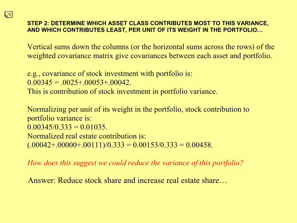
STEP 2: DETERMINE WHICH ASSET CLASS CONTRIBUTES MOST TO THIS VARIANCE, AND WHICH CONTRIBUTES LEAST, PER UNIT OF ITS WEIGHT IN THE PORTFOLIO… Vertical sums down the columns (or the horizontal sums across the rows) of the weighted covariance matrix give covariances between each asset and portfolio. e.g., covariance of stock investment with portfolio is: 0.00345 = .0025+.00053+.00042. This is contribution of stock investment in portfolio variance. Normalizing per unit of its weight in the portfolio, stock contribution to portfolio variance is: 0.00345/0.333 = 0.01035. Normalized real estate contribution is: (.00042+.00000+.00111)/0.333 = 0.00153/0.333 = 0.00458. How does this suggest we could reduce the variance of this portfolio?

Answer: Reduce stock share and increase real estate share…

Thus, per unit of weight in the portfolio, the marginal contribution of each asset in the portfolio’s variance is proportional to the asset’s covariance with the portfolio.

STEP 3: TRY VARIOUS COMBINATIONS OF ASSET CLASS WEIGHTS UNTIL MINIMUM-VARIANCE COMBINATION IS FOUND (SUBJECT TO TARGET RETURN CONSTRAINT)… Repeat the above steps, modifying the asset weights according to an efficient algorithm, increasing asset classes that reduce variance and decreasing those that increase variance, in proportions so as to preserve the 9% portfolio return =wST12% + wBD7% + wRE8% = 9% target. Computer’s “Solver” has an algorithm to do this efficiently, and can work very fast.

STEP 4: IF YOU WANT TO GENERATE THE ENTIRE “EFFICIENT FRONTIER”, THEN REPEAT THE ABOVE STEPS FOR A SERIES OF DIFFERENT TARGET RETURNS…

THE EFFICIENT FRONTIER USING OUR PREVIOUS RISK/RETURN ASSUMPTIONS FOR THE THREE MAJOR ASSET CLASSES: Three asset efficient frontier, given: Input data assumptions:

Stocks Bonds REMean Return 12.00% 7.00% 8.00%STD (vol.) 15.00% 8.00% 10.00%Correlation: Stocks 100.00% 40.00% 25.00%Bonds 100.00% 0.00%RE 100.00%Efficient Frontier: E(rP) sP StockSh BondSh REShare

7.39% 6.25% 0.00% 60.98% 39.02%7.90% 6.48% 10.32% 51.02% 38.66%8.41% 7.01% 20.76% 41.59% 37.64%8.93% 7.76% 31.21% 32.16% 36.63%9.44% 8.67% 41.66% 22.73% 35.61%9.95% 9.71% 52.11% 13.30% 34.60%

10.46% 10.84% 62.55% 3.87% 33.58%10.98% 12.06% 74.39% 0.00% 25.61%11.49% 13.46% 87.20% 0.00% 12.80%12.00% 15.00% 100.00% 0.00% 0.00%

(See if you can get the “portfo1.xls” spreadsheet to generate this efficient frontier using the Excel Solver...)

Through here 2nd class

SOME NAGGING QUESTIONS ABOUT MPT . . .

HOW SENSITIVE ARE THE RESULTS TO OUR INPUT ASSUMPTIONS (RISK & RETURN EXPECTATIONS), AND HOW REALISTIC ARE THOSE EXPECTATIONS?

WHAT IS LEFT OUT OF THIS MODEL, AND HOW COULD YOU TRY TO INCORPORATE THESE OMISSIONS?

- TRANSACTION COSTS?- LIQUIDITY CONCERNS?

CAN YOU "GAME" PORTFOLIO THEORY BY REDEFINING THE NUMBER AND DEFINITION OF "ASSET CLASSES"?

Watch out for “silly” results (e.g., putting conservative investors in poor performing investments). When applying portfolio theory, don’t check your common sense at the door.

FOR EXAMPLE, DOES IT REALLY MAKE SENSE TO PUT SO LITTLE INTO STOCKS JUST BECAUSE YOU HAVE A CONSERVATIVE RETURN TARGET, EVEN THOUGH STOCKS PROVIDE A SUPERIOR RETURN RISK PREMIUM PER UNIT OF RISK?…

WHAT ABOUT LEVERAGE?...

SOME OF THESE QUESTIONS CAN BE ADDRESSED BY A NEAT TRICK, AN EXTENSION TO THE ABOVE-DESCRIBED PORTFOLIO THEORY...

VII. INTRODUCING A "RISKLESS ASSET"... IN A COMBINATION OF A RISKLESS AND A RISKY ASSET, BOTH RISK AND RETURN ARE WEIGHTED AVERAGES OF RISK AND RETURN OF THE TWO ASSETS: Recall: sP = √[ ω²(si)² + (1-ω)²(sj)² + 2ω(1-ω)sisjCij ] If sj=0, this reduces to: sP = √[ ω²(si)² = ωsi SO THE RISK/RETURN COMBINATIONS OF A MIXTURE OF INVESTMENT IN A RISKLESS ASSET AND A RISKY ASSET LIE ON A STRAIGHT LINE, PASSING THROUGH THE TWO POINTS REPRESENTING THE RISK/RETURN COMBINATIONS OF THE RISKLESS ASSET AND THE RISKY ASSET.

IN PORTFOLIO ANALYSIS, THE "RISKLESS ASSET" REPRESENTS BORROWING OR LENDING BY THE INVESTOR… BORROWING IS LIKE "SELLING SHORT" OR HOLDING A NEGATIVE WEIGHT IN THE RISKLESS ASSET. BORROWING IS "RISKLESS" BECAUSE YOU MUST PAY THE MONEY BACK “NO MATTER WHAT”. LENDING IS LIKE BUYING A BOND OR HOLDING A POSITIVE WEIGHT IN THE RISKLESS ASSET. LENDING IS "RISKLESS" BECAUSE YOU CAN INVEST IN GOVT BONDS AND HOLD TO MATURITY.

SUPPOSE YOU COMBINE RISKLESS BORROWING OR LENDING WITH YOUR INVESTMENT IN THE RISKY PORTFOLIO OF STOCKS & REAL ESTATE. YOUR OVERALL EXPECTED RETURN WILL BE: rW = vrP + (1-v)rf AND YOUR OVERALL RISK WILL BE: sW = vsP + (1-v)0 = vsP Where: v = Weight in risky portfolio rW, sW = Return, Std.Dev., in overall wealth rP, sP = Return, Std.Dev., in risky portfolio rf = Riskfree Interest Rate v NEED NOT BE CONSTRAINED TO BE LESS THAN UNITY. v CAN BE GREATER THAN 1 ("leverage" , "borrowing"), OR v CAN BE LESS THAN 1 BUT POSITIVE ("lending", investing in bonds, in addition to investing in the risky portfolio). THUS, USING BORROWING OR LENDING, IT IS POSSIBLE TO OBTAIN ANY RETURN TARGET OR ANY RISK TARGET. THE RISK/RETURN COMBINATIONS WILL LIE ON THE STRAIGHT LINE PASSING THROUGH POINTS rf AND rP.

NUMERICAL EXAMPLE SUPPOSE: RISKFREE INTEREST RATE = 5% STOCK EXPECTED RETURN = 15% STOCK STD.DEV. = 15% ________________________________________________________ IF RETURN TARGET = 20%, BORROW $0.5 INVEST $1.5 IN STOCKS (v = 1.5). EXPECTED RETURN WOULD BE: (1.5)15% + (-0.5)5% = 20% RISK WOULD BE (1.5)15% + (-0.5)0% = 22.5% ________________________________________________________ IF RETURN TARGET = 10%, LEND (INVEST IN BONDS) $0.5 INVEST $0.5 IN STOCKS (v = 0.5). EXPECTED RETURN WOULD BE: (0.5)15% + (0.5)5% = 10% RISK WOULD BE (0.5)15% + (0.5)0% = 7.5% ___________________________________________________________

NOTICE THESE POSSIBILITIES LIE ON A STRAIGHT LINE IN RISK/RETURN SPACE . . .

0% 7.5% 15% 22.5%0%

5%

10%

15%

20%

25%

30%

35%RISK & RETURN COMBINATIONS USING STOCKS & RISKLESS BORROWING OR LENDI

RISK (STD.DEV.)

EXPCTEDRETURN

V = WEIGHT IN STOCKSV=0

V=50%

V=150%

V=100%

BORROW

LEND

BUT NO MATTER WHAT YOUR RETURN TARGET, YOU CAN DO BETTER BY PUTTING YOUR RISKY MONEY IN A DIVERSIFIED PORTFOLIO OF REAL ESTATE & STOCKS . . . SUPPOSE: REAL ESTATE EXPECTED RETURN = 10% REAL ESTATE STD.DEV. = 10% CORRELATION BETWEEN STOCKS & REAL ESTATE = 25% THEN 50% R.E. / STOCKS MIXTURE WOULD PROVIDE: EXPECTED RETURN = 12.5%; STD.DEV. = 10.0% ________________________________________________________ IF RETURN TARGET = 20%, BORROW $1.0 INVEST $2.0 IN RISKY MIXED-ASSET PORTFOLIO (v = 2). EXPECTED RETURN WOULD BE: (2.0)12.5% + (-1.0)5% = 20% RISK WOULD BE: (2.0)10.0% + (-1.0)0% = 20% < 22.5% _______________________________________________________ IF RETURN TARGET = 10%, LEND (INVEST IN BONDS) $0.33 INVEST $0.67 IN RISKY MIXED-ASSET PORTFOLIO (v = 0.67). EXPECTED RETURN WOULD BE: (0.67)12.5% + (0.33)5% = 10% RISK WOULD BE: (0.67)10.0% + (0.33)0% = 6.7% < 7.5%

THE GRAPH BELOW SHOWS THE EFFECT DIVERSIFICATION IN THE RISKY PORTFOLIO HAS ON THE RISK/RETURN POSSIBILITY FRONTIER.

0%

5%

10%

15%

20%

25%

0% 5% 10% 15% 20% 25%Risk in overall wealth portfolio

Expt

d R

etur

n

Effect of diversif ication: Stocks, R.E., & Riskless Asset

THE FRONTIER IS STILL A STRAIGHT LINE ANCHORED ON THE RISKFREE RATE, BUT THE LINE NOW HAS A GREATER “SLOPE”, PROVIDING MORE RETURN FOR THE SAME AMOUNT OF RISK, ALLOWING LESS RISK FOR THE SAME EXPECTED RETURN.

THE "OPTIMAL" RISKY ASSET PORTFOLIO WITH A RISKLESS ASSET

(aka "TWO-FUND THEOREM")

CURVED LINE IS FRONTIER OBTAINABLE INVESTING ONLY IN RISKY ASSETS STRAIGHT LINE PASSING THRU rf AND PARABOLA IS OBTAINABLE BY MIXING RISKLESS ASSET (LONG OR SHORT) WITH RISKY ASSETS. YOU WANT “HIGHEST” STRAIGHT LINE POSSIBLE (NO MATTER WHO YOU ARE!). OPTIMAL STRAIGHT LINE IS THUS THE ONE PASSING THRU POINT "P". IT IS THE STRAIGHT LINE ANCHORED IN rf WITH THE MAXIMUM POSSIBLE SLOPE. THUS, THE STRAIGHT LINE PASSING THROUGH “P” IS THE EFFICIENT FRONTIER. THE FRONTIER TOUCHES (AND INCLUDES) THE CURVED LINE AT ONLY ONE POINT: THE POINT "P".

rf

i

jP

rjrP

ri

Risk(Std.Dev.of Portf)

E[Return]

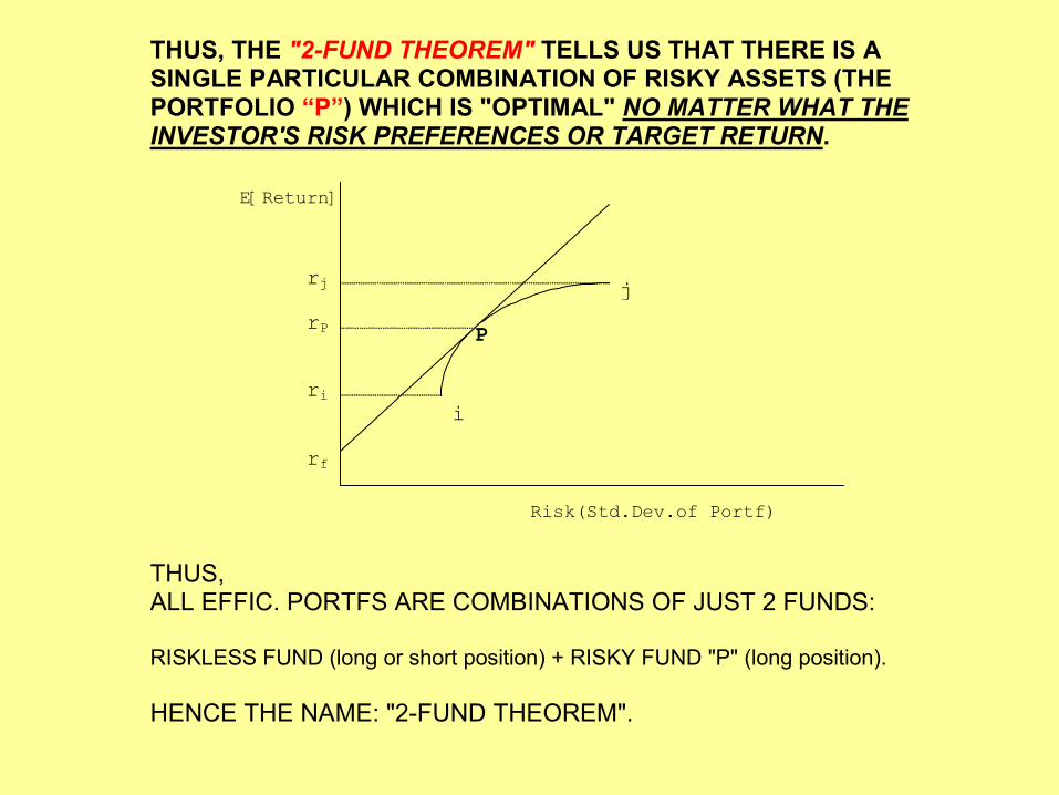
THUS, THE "2-FUND THEOREM" TELLS US THAT THERE IS A SINGLE PARTICULAR COMBINATION OF RISKY ASSETS (THE PORTFOLIO “P”) WHICH IS "OPTIMAL" NO MATTER WHAT THE INVESTOR'S RISK PREFERENCES OR TARGET RETURN.

THUS, ALL EFFIC. PORTFS ARE COMBINATIONS OF JUST 2 FUNDS: RISKLESS FUND (long or short position) + RISKY FUND "P" (long position). HENCE THE NAME: "2-FUND THEOREM".

rf

i

j P

rjrP

ri

Risk(Std.Dev.of Portf)

E[Return]

HOW DO WE KNOW WHICH COMBINATION OF RISKY ASSETS IS THE OPTIMAL ALL-RISKY PORTFOLIO “P”? IT IS THE ONE THAT MAXIMIZES THE SLOPE OF THE STRAIGHT LINE FROM THE RISKFREE RETURN THROUGH “P”. THE SLOPE OF THIS LINE IS GIVEN BY THE RATIO: Portfolio Sharpe Ratio = (rp - rf) / sP MAXIMIZING THE SHARPE RATIO FINDS THE OPTIMAL RISKY ASSET COMBINATION. THE SHARPE RATIO IS ALSO A GOOD INTUITIVE MEASURE OF “RISK-ADJUSTED RETURN” FOR THE INVESTOR’S WEALTH, AS IT GIVES THE RISK PREMIUM PER UNIT OF RISK (MEASURED BY ST.DEV). THUS, IF WE ASSUME THE EXISTENCE OF A RISKLESS ASSET, WE CAN USE THE 2-FUND THEOREM TO FIND THE OPTIMAL RISKY ASSET MIXTURE AS THAT PORTFOLIO WHICH HAS THE HIGHEST "SHARPE RATIO".

BACK TO PREVIOUS 2-ASSET NUMERICAL EXAMPLE... USING OUR PREVIOUS EXAMPLE NUMBERS, THE OPTIMAL COMBINATION OF REAL ESTATE & STOCKS CAN BE FOUND BY EXAMINING THE SHARPE RATIO FOR EACH COMBINATION . . . ω = RE share

rP rp-rf sP SharpeRatio

0 15.0% 10.0% 15.0% 66.7%0.1 14.5% 9.5% 13.8% 68.9%0.2 14.0% 9.0% 12.6% 71.2%0.3 13.5% 8.5% 11.6% 73.2%0.4 13.0% 8.0% 10.7% 74.6%0.5 12.5% 7.5% 10.0% 75.0%0.6 12.0% 7.0% 9.5% 73.8%0.7 11.5% 6.5% 9.2% 70.5%0.8 11.0% 6.0% 9.2% 65.1%0.9 10.5% 5.5% 9.5% 58.0%1.0 10.0% 5.0% 10.0% 50.0% OF THE 11 MIXTURES CONSIDERED ABOVE, THE 50% REAL ESTATE WOULD BE BEST BECAUSE IT HAS THE HIGHEST SHARPE MEASURE. BUT SUPPOSE YOU ARE NOT SATISFIED WITH THE 12.5% Er THAT WILL GIVE YOU FOR YOUR OVERALL WEALTH? … OR YOU DON’T WANT TO SUBJECT YOUR OVERALL WEALTH TO 10% VOLATILITY?...

THEN YOU CAN INVEST PROPORTIONATELY 50% IN REAL ESTATE AND 50% IN STOCKS, … AND THEN ACHIEVE A GREATER RETURN THAN 12.5% BY BORROWING (LEVERAGE, v > 1), OR YOU CAN INCUR LESS THAN 10.0% RISK BY LENDING (INVESTING IN GOVT BONDS, v<1)… (BUT YOU CAN’T DO BOTH. THE “FREE LUNCH” OF PORTFOLIO THEORY ONLY GETS YOU SO FAR, THAT IS, TO THE EFFICIENT FRONTIER, BUT ON THAT FRONTIER THERE WILL BE A RISK/RETURN TRADEOFF. THAT TRADEOFF WILL BE DETERMINED BY THE MARKET…)

2-FUND THEOREM SUMMARY: 1) THE 2-FUND THEOREM ALLOWS AN ALTERNATIVE,

INTUITIVELY APPEALING DEFINITION OF THE OPTIMAL RISKY PORTFOLIO: THE ONE WITH THE MAXIMUM SHARPE RATIO.

2) THIS CAN HELP AVOID "SILLY" OPTIMAL PORTFOLIOS

THAT PUT TOO LITTLE WEIGHT IN HIGH-RETURN ASSETS JUST BECAUSE THE INVESTOR HAS A CONSERVATIVE TARGET RETURN. (OR TOO LITTLE WEIGHT IN LOW-RETURN ASSETS JUST BECAUSE THE INVESTOR HAS AN AGGRESSIVE TARGET.)

3) IT ALSO PROVIDES A GOOD FRAMEWORK FOR

ACCOMMODATING THE POSSIBLE USE OF LEVERAGE, OR OF RISKLESS INVESTING (BY HOLDING BONDS TO MATURITY), BY THE INVESTOR.

Chapter 21 Summary: MPT & Real Estate . . .Chapter 21 Summary: MPT & Real Estate . . .•• The classical theory suggests a fairly robust, substantial roleThe classical theory suggests a fairly robust, substantial role for the real estate for the real estate asset class in the optimal portfolio (typically 25%asset class in the optimal portfolio (typically 25%--40% without any additional 40% without any additional assumptions), either w or w/out assumptions), either w or w/out risklessriskless asset.asset.•• This role tends to be greater for more conservative portfolios,This role tends to be greater for more conservative portfolios, less for very less for very aggressive portfolios.aggressive portfolios.•• Role is based primarily on Role is based primarily on diversification benefitsdiversification benefits of real estate, somewhat of real estate, somewhat sensitive to R.E. correlation w stocks & bonds.sensitive to R.E. correlation w stocks & bonds.•• Optimal real estate share roughly matches actual real estate prOptimal real estate share roughly matches actual real estate proportion of all oportion of all investableinvestable assets in the economy.assets in the economy.•• Optimal real estate share in theory is substantially greater thOptimal real estate share in theory is substantially greater than actual pension an actual pension fund allocations to real estate.fund allocations to real estate.•• Optimal R.E. share can be reduced by adding assumptions and extOptimal R.E. share can be reduced by adding assumptions and extensions to the ensions to the classical model:classical model:

• Extra transaction costs, illiquidity penalties;• Long-term horizon risk & returns;• Net Asset-Liability portfolio framework;• Investor constrained to over-invest in owner-occupied house as investment.

•• But even with such extensions, optimal R.E. share often substanBut even with such extensions, optimal R.E. share often substantially exceeds tially exceeds existing P.F. allocations to R.E. (approx. 3% on avg.*)existing P.F. allocations to R.E. (approx. 3% on avg.*)

* This average includes a large number of (mostly smaller) pension funds that have no allocation to real estate at all. Some of the larger funds have allocation targets in the 8% - 10% range, which is not far out of line with what the theory indicates if you include some of the added assumptions and extensions noted here.

VIII. FROM PORTFOLIO THEORY TO EQUILIBRIUM ASSET PRICE MODELLING...

HOW ASSET MARKET PRICES ARE DETERMINED. i.e., WHAT SHOULD BE “E[r]” FOR ANY GIVEN ASSET?… RECALL RELATION BETW “PV” AND “E[r]”.

e.g., for perpetutity: PV = CF / E[r]

(A model of price is a model of expected return, and vice versa, a model of expected return is a model of price.)

THUS, ASSET PRICING MODEL CAN IDENTIFY “MISPRICED” ASSETS (ASSETS WHOSE “E[r]” IS ABOVE OR BELOW WHAT IT SHOULD BE, THAT IS, ASSETS WHOSE CURRENT “MVs” ARE “WRONG”, AND WILL PRESUMABLY TEND TO “GET CORRECTED” IN THE MKT OVER TIME). IF PRICE (HENCE E[r]) OF ANY ASSET DIFFERS FROM WHAT THE MODEL PREDICTS, THE IMPLICATION IS THAT THE PRICE OF THAT ASSET WILL TEND TO REVERT TOWARD WHAT THE MODEL PREDICTS, THEREBY ALLOWING PREDICTION OF SUPER-NORMAL OR SUB-NORMAL RETURNS FOR SPECIFIC ASSETS, WITH OBVIOUS INVESTMENT POLICY IMPLICATIONS.

Quick & simple example… Suppose model predicts E[r] for $10 perpetuity asset should be 10%. This means equilibrium price of this asset should be $100. But you find an asset like this whose price is $83. This means it is providing an E[r] of 12% ( = 10 / 83 ). Thus, if model is correct, you should buy this asset for $83. Because at that price it is providing a “supernormal” return, and because we would expect that as prices move toward equilibrium the value of this asset will move toward $100 from its current $83 price. (i.e., You will get your supernormal return either by continuing to receive a 12% yield when the risk only warrants a 10% yield, or else by the asset price moving up in equilibrium providing a capital gain “pop”.)

Obviously the $10 payments are risky. (Through here 3rd day)

THE "SHARPE-LINTNER CAPM" (in 4 easy steps!)… (Nobel prize-winning stuff here – Show some respect!) 1ST) 2-FUND THEOREM SUGGESTS THERE IS A SINGLE COMBINATION OF RISKY ASSETS THAT YOU SHOULD HOLD, NO MATTER WHAT YOUR RISK PREFERENCES. THUS, ANY INVESTORS WITH THE SAME EXPECTATIONS ABOUT ASSET RETURNS WILL WANT TO HOLD THE SAME RISKY PORTFOLIO (SAME COMBINATION OR RELATIVE WEIGHTS).

2ND) GIVEN INFORMATIONAL EFFICIENCY IN SECURITIES MARKET, IT IS UNLIKELY ANY ONE INVESTOR CAN HAVE BETTER INFORMATION THAN THE MARKET AS A WHOLE, SO IT IS UNLIKELY THAT YOUR OWN PRIVATE EXPECTATIONS CAN BE SUPERIOR TO EVERY ONE ELSE'S. THUS, EVERYONE WILL CONVERGE TO HAVING THE SAME EXPECTATIONS, LEADING EVERYONE TO WANT TO HOLD THE SAME PORTFOLIO. THAT PORTFOLIO WILL THEREFORE BE OBSERVABLE AS THE "MARKET PORTFOLIO", THE COMBINATION OF ALL THE ASSETS IN THE MARKET, IN VALUE WEIGHTS PROPORTIONAL TO THEIR CURRENT CAPITALIZED VALUES IN THE MARKET.

3RD) SINCE EVERYBODY HOLDS THIS SAME PORTFOLIO, THE ONLY RISK THAT MATTERS TO INVESTORS, AND THEREFORE THE ONLY RISK THAT GETS REFLECTED IN EQUILIBRIUM MARKET PRICES, IS THE COVARIANCE WITH THE MARKET PORTFOLIO. (Recall that the contribution of an asset to the risk of a portfolio is the covariance betw that asset & the portf.) THIS COVARIANCE, NORMALIZED SO IT IS EXPRESSED PER UNIT OF VARIANCE IN THE MARKET PORTFOLIO, IS CALLED "BETA".

Another way of looking at this is that the market represents the “average” investor (or the most “representative” investor, the one who stands for the market as a whole). The risk that matters to this average or representative investor in considering any specific asset is only that asset’s covariance with the rest of this investor’s portfolio, namely, the covariance with the market. This covariance equals that asset’s contribution to the risk of the investor’s overall wealth portfolio. Let COV(i,M) = covariance betw asset i’s return and the market return; VAR(M) = the market return’s variance. Then, for the average or representative investor, VAR(M) is the risk in his/her wealth portfolio, and COV(i,M) is the effective risk in Asset i (as this asset would contribute to the risk in the average investor’s wealth portfolio). If (ErM-rf) is the market risk premium that effectively compensates the average (marginal) investor for the amount of risk in their wealth, then [COV(i,M)/VAR(M)](ErM-rf) should be the required risk premium for Asset i so that it provides the same risk premium per unit of effective risk as the rest of the investor’s wealth portfolio. (Otherwise, we are not in equilibrium: the investor would want to either purchase more of Asset i if it provided greater expected return per unit of risk (necessitating a sale of the rest of the market portfolio), or else he/she would want to sell Asset i short or get rid of it from their wealth portfolio, in contrast to the current equilibrium reality in which Asset i finds itself in the wealth portfolio of Mr/Mrs Average.) Note that [COV(i,M)/VAR(M)] is the definition of “beta”.

4TH) THEREFORE, IN EQUILIBRIUM, ASSETS WILL REQUIRE AN EXPECTED RETURN EQUAL TO THE RISKFREE RATE PLUS THE MARKET'S RISK PREMIUM TIMES THE ASSET'S BETA:

E[ri] = rf + RPi = rf + βi(ErM - rf)

Let COV(i,M) = covariance betw asset i’s return and the market return; VAR(M) = the market return’s variance. Then, for the average or representative investor, VAR(M) is the risk in his/her wealth portfolio, and COV(i,M) is the effective risk in Asset i (as this asset would contribute to the risk in the average investor’s wealth portfolio). If (ErM-rf) is the market risk premium, that effectively compensates the average (marginal) investor for the amount of risk in their wealth, then [COV(i,M)/VAR(M)](ErM-rf) should be the required risk premium for Asset i so that it provides the same risk premium per unit of effective risk as the rest of the investor’s wealth portfolio. (Otherwise, we are not in equilibrium: the investor would want to either purchase more of Asset i if it provided greater expected return per unit of risk (necessitating a sale of the rest of the market portfolio), or else he/she would want to sell Asset i short or get rid of it from their wealth portfolio, in contrast to the current equilibrium reality in which Asset i finds itself in the wealth portfolio of Mr/Mrs Average.) Note that [COV(i,M)/VAR(M)] is the definition of “beta”.

THE CAPM IS OBVIOUSLY A SIMPLIFICATION (of reality)… (Yes, I know that markets are not really perfectly efficient. I know we don’t all have the same expectations. I know we do not all really hold the same portfolios.) BUT IT IS A POWERFUL AND WIDELY-USED MODEL. IT CAPTURES AN IMPORTANT PART OF THE ESSENCE OF REALITY ABOUT ASSET MARKET PRICING…

Conceptually: Asset markets are “pretty efficient” (most of the time). Many investors (especially large institutions) hold very similar

portfolios. Investors who determine market prices are those who are buying

and selling in the asset market, and “on average” (in some vague sense) those investors “ARE the market”. In other words, if there were just one giant investor, whose name was “the market”, then the CAPM would explain the prices (and expected) returns that investor would pay (and require), if that giant investor were “rational”.

Models ARE SUPPOSED TO “simplify” reality, enabling us to gain insight and understanding from the “jumble of too-many facts” that is reality. Empirically:

The CAPM works (pretty well, not perfectly) for explaining stock prices (stock average returns across time), using the stock market itself as a proxy for the “market portfolio”.

APPLYING THE CAPM TO REAL ESTATE… (WE NEED TO CONSIDER REITs & “DIRECT” PRIVATE REAL ESTATE SEPARATELY…) THE CAPM IS TRADITIONALLY APPLIED ONLY TO THE STOCK MARKET. THE "MARKET PORTFOLIO" (THE INDEX ON WHICH "BETA" IS DEFINED) IS TRADITIONALLY PROXIED BY THE STOCK MARKET.

(FIRST, CONSIDER REITs…)

THIS TRADITIONAL APPLICATION WORKS ABOUT AS WELL FOR REITs AS IT DOES FOR OTHER STOCKS. CAVEAT APPLYING TRADITIONAL CAPM TO REITs... IN GENERAL, REITs ARE LOW-BETA STOCKS, AND MANY REITs ARE SMALL STOCKS. THE CAPM TENDS TO UNDER-PREDICT THE AVERAGE RETURNS TO LOW-BETA STOCKS AND SMALL STOCKS, INCLUDING REITs.

This relates to the famous “Fama-French Factors”: Market Capitalization, and the Market/Book Ratio. Stocks with smaller market capitalizations and smaller market/book value ratios tend to provide greater average returns than their betas alone would suggest. Small stocks and stocks with low mkt/book ratios may tend to be more susceptible to catastrophic failure, especially in the event of bad economic times or major financial crises. The “non-normal” event risk that is not well captured in periodic return series covariance (beta) may be correlated with these Fama-French factors.

•• THE SMALL STOCK EFFECT MAY BE DUE TO GREATER THE SMALL STOCK EFFECT MAY BE DUE TO GREATER SENSITIVITY OF SMALL STOCK RETURNS TO THE SENSITIVITY OF SMALL STOCK RETURNS TO THE BUSINESS CYCLE, PARTICULARLY EXTREME DOWNSIDE BUSINESS CYCLE, PARTICULARLY EXTREME DOWNSIDE RETURN SENSITIVITY TO RECESSIONS. RETURN SENSITIVITY TO RECESSIONS.

•• INVESTORS CARE ABOUT BUSINESS CYCLE RISK INVESTORS CARE ABOUT BUSINESS CYCLE RISK BECAUSE THEIR OWN HUMAN CAPITAL VALUE AND BECAUSE THEIR OWN HUMAN CAPITAL VALUE AND CONSUMPTION IS POSITIVELY CORRELATED WITH THE CONSUMPTION IS POSITIVELY CORRELATED WITH THE BUSINESS CYCLE. BUSINESS CYCLE.

•• A STOCK THAT IS SENSITIVE TO THE BUSINESS CYCLE A STOCK THAT IS SENSITIVE TO THE BUSINESS CYCLE WILL NOT HEDGE THAT RISK AND MAY IN FACT WILL NOT HEDGE THAT RISK AND MAY IN FACT EXACERBATE IT. EXACERBATE IT.

•• HOWEVER, IT IS NOT CLEAR THAT HOWEVER, IT IS NOT CLEAR THAT REITsREITs ARE TYPICAL ARE TYPICAL OF OTHER SMALL STOCKS IN THIS REGARD.OF OTHER SMALL STOCKS IN THIS REGARD.

Possible reasons for REIT out-performance of the CAPM prediction in equilibrium: As high-dividend yield stocks, REIT returns face a higher effective tax rate than growth stocks. There is also evidence that REIT betas are larger in down-markets than in up-markets. And small stocks may also be subject to an “illiquidity premium” in the stock market.

(NEXT, CONSIDER PRIVATE REAL ESTATE…) TRADITIONAL CAPM, BASED ON THE STOCK MARKET AS THE "BETA" INDEX, DOES NOT WORK WELL FOR PRIVATE REAL ESTATE… PRIVATE REAL ESTATE RETURNS ARE NOT HIGHLY CORRELATED WITH STOCK MARKET. THIS GIVES REAL ESTATE A VERY LOW "BETA" (MEASURED WRT STOCK MARKET). YET REAL ESTATE IS GENERALLY VIEWED AS A “RISKY INVESTMENT” MERRITING (AND GETTING) A SUBSTANTIAL RISK PREMIUM IN ITS EX ANTE RETURN. THUS, TRADITIONAL APPLICATION OF CAPM DOES NOT SEEM TO WORK FOR PRIVATE REAL ESTATE…

rf

β

E[r]

CAPM Prediction

rRE

Actual R.E. return

(ANYWAY, THIS IS THE TRADITIONAL “COMPLAINT” ABOUT THE CAPM AS IT RELATES TO PRIVATE REAL ESTATE.)

ASIDE: IS THIS TRADITIONAL COMPLAINT REALLY BORN OUT BY THE EMPIRICAL EVIDENCE?…

SO-CALLED "INSTITUTIONAL QUALITY" COMMERCIAL PROPERTY HAS PROVIDED ONLY A VERY SMALL RISK PREMIUM OVER THE PAST COUPLE OF DECADES, ABOUT THE SAME AS LONG-TERM BONDS, FOR EXAMPLE.

MANY OF THE "INSTITUTIONS" WHO INVEST IN SUCH PROPERTY (SUCH AS PENSION FUNDS AND LIFE INSURANCE COMPANIES) HAVE OVERALL PORTFOLIOS THAT ARE DOMINATED BY STOCKS AND BONDS, ASSETS WITH WHICH PRIVATE REAL ESTATE HAS LOW CORRELATION. THUS, THE TRADITIONAL CAPM MAY INDEED WORK WELL FOR “INSTITUTIONAL” REAL ESTATE…

SUCH INVESTORS WOULD BE SATISFIED WITH LOW RISK PREMIUMS IN REAL ESTATE, BECAUSE OF THE DIVERSIFICATION ROLE REAL ESTATE PLAYS IN THEIR OVERALL PORTFOLIOS.

ON THE OTHER HAND, NON-INSTITUTIONAL REAL ESTATE, INCLUDING HOUSING, SEEMS GENERALLY TO HAVE PROVIDED A SUBSTANTIAL RISK PREMIUM ON AVERAGE, THOUGH THIS IS DIFFICULT TO QUANTIFY RELIABLY.

MUCH OF THIS NON-INSTITUTIONAL REAL ESTATE MAY BE OWNED BY INVESTORS WHO ARE NOT SO WELL DIVERSIFIED, AND MAY HAVE A SUBSTANTIAL FRACTION OF THEIR OVERALL WEALTH IN THEIR REAL ESTATE INVESTMENTS. THIS WOULD MAKE SUCH INVESTORS NEED A HIGH RISK PREMIUM FROM REAL ESTATE, BASED PURELY ON ITS VOLATILITY, AS ITS LOW CORRELATION WITH STOCKS AND BONDS WOULD NOT HELP THEM OUT. SO, IT WOULD MAKE SENSE THAT THE TRADITIONAL CAPM WOULD NOT HOLD FOR NON-INSTITUTIONAL PRIVATE REAL ESTATE.

CAN THE CAPM BE APPLIED MORE BROADLY TO ENCOMPASS ALL PRIVATE REAL ESTATE AS WELL AS PUBLICLY-TRADED SECURITIES SUCH AS STOCKS AND REITs?… ACCORDING TO THE CAPM THEORY, THE "MARKET PORTFOLIO" ON WHICH "BETA" (AND HENCE THE EXPECTED RETURN RISK PREMIUM) IS BASED SHOULD INCLUDE ALL THE ASSETS IN THE ECONOMY. THIS SHOULD INCLUDE, IN ADDITION TO STOCKS AND BONDS, REAL ESTATE ITSELF, AS WELL AS INVESTORS' OWN "HUMAN CAPITAL", AND OTHER NON-TRADABLE ASSETS. THERE IS SOME EVIDENCE THAT IF ONE MEASURES PRIVATE REAL ESTATE'S "BETA" IN THIS WAY, BASED ON A BROADER MARKET PORTFOLIO (OR BASED ON NATIONAL CONSUMPTION), THEN REAL ESTATE HAS A SUBSTANTIALLY POSITIVE BETA, PROBABLY AT LEAST HALF THAT OF THE STOCK MARKET. THUS, A MORE BROADLY APPLIED CAPM WOULD SEEM TO SUGGEST THAT PRIVATE REAL ESTATE DOES REQUIRE A SUBSTANTIAL RISK PREMIUM IN ITS EXPECTED RETURN. ON AVERAGE, INCLUDING BOTH INSTITUTIONAL AND NON-INSTITUTIONAL REAL ESTATE, PRIVATE REAL ESTATE PROBABLY DOES PROVIDE SUCH A RISK PREMIUM.

Another perspective on the relevance of the CAPM to real estate:Another perspective on the relevance of the CAPM to real estate: Distinguish Distinguish between applications between applications WithinWithin the institutional private R.E. asset classthe institutional private R.E. asset class,, versus versus applications: applications: AcrossAcross broad asset classes (“mixed asset portfolio” level)broad asset classes (“mixed asset portfolio” level) . .. . ..

NCREIF Division/Type Portfolios: Returns vs NWP Factor Risk

-1.5%

-1.0%

-0.5%

0.0%

0.5%

1.0%

1.5%

-0.5 0.0 0.5 1.0 1.5

Beta w rt NWP=(1/3)St+(1/3)Bn+(1/3)RE

Avg

Exc

ess

Retu

rn (o

vr T

-bills

)

No relationship between CAPM-defined risk and cross-section of ex post returns.

In this plot, institutional real estate portfolio returns (actually, NCREIF sub-index returns) are plotted against beta computed with respect to the “National Wealth Portfolio” (which consists stylistically of (1/3) stocks, (1/3) bonds, and (1/3) real estate). But it does not matter how we compute the “beta”. (For example, we can compute it with respect to the stock market, the NCREIF Index, National Consumption, whatever…) There is no ex post relationship between risk and return. This means that there is no significant distinction in ex ante real estate risk premia for different types or locations of (institutional quality) commercial property, within the private property market. In other words, the cross-section of expected returns across property types & locations is essentially FLAT (within the institutional quality asset class). (See Chapter 22, section 22.3, pp.573-583.)

Ex Post CAPM on Mkt=(1/3)RE+(1/3)Bonds+(1/3)Stocks

0.0%

1.0%

2.0%

3.0%

0 0.5 1 1.5 2 2.5

Beta* RE betas = sum of 8qtrs lagged coeffs

Avg

Exc

ess

Retu

rn (p

er q

tr, o

ver T

bills

)

NCREIF

LTBond

SP500

HOUSCMORT

REIT

SMALST

But the CAPM appears to be more meaningful when we But the CAPM appears to be more meaningful when we take a broader perspective take a broader perspective ACROSSACROSS asset classes. . .asset classes. . .

Look at this regression of asset class ex post returns onto their betas with respect to the National Wealth Portfolio, as it was previously stylistically defined (equal shares of stocks, bonds and real estate). This scatter plot looks very different from the one we previously looked at within the private equity quadrant.

Regression statistics for historical returns Regression statistics for historical returns ACROSSACROSS asset asset classes . . .classes . . .

Ex Post CAPM on Mkt=(1/3)RE+(1/3)Bonds+(1/3)Stocks

0.0%

1.0%

2.0%

3.0%

0 0.5 1 1.5 2 2.5

Beta* RE betas = sum of 8qtrs lagged coeffs

Avg

Exc

ess

Retu

rn (p

er q

tr, o

ver T

bills

)

NCREIF

LTBond

SP500

HOUSCMORT

REIT

SMALST

•Adj. R2 = 73%

• Intercept is Insignif.

•Coeff on Beta is Pos & Signif.

“CAPM works...”“CAPM works...”

Here, at this ACROSS-ASSET CLASS level, the historical empirical evidence is quite strong. Adjusted R-square is a very robust 73%. The “intercept” is insignificant (which is exactly what we expect when we have a good model of risk and return). The coefficient on beta is positive & significant. In other words, “Beta” with respect to the “National Wealth” is priced ACROSS the asset classes. A National Wealth-based CAPM “works” pretty well at this broad-brush level. [See Chapter 22, section 22.2, especially pp.568-572, Exh.22-2b on p.571.]

The Capital Market does perceive (and price) risk differences The Capital Market does perceive (and price) risk differences ACROSSACROSS asset classes . . .asset classes . . .

National Wealth BETABETA

Pub.EqPub.Eq

Pub.DbPub.Db

Pri.DbPri.Db

Pri.EqPri.Eq

Real estate based asset classes: Property, Mortgages, CMBS, Real estate based asset classes: Property, Mortgages, CMBS, REITsREITs……

Apparently, the capital market does perceive and price risk differences ACROSS the quadrants. Within real estate based asset classes: PRIV EQ (direct property, unlevered) is the low-beta class. PUBL EQ (REITs) is the high-beta quad. DEBT lies in between.

Asset Class Ex Post Betas and Risk Asset Class Ex Post Betas and Risk PremiaPremia (Per (Per Annum, over TAnnum, over T--bills, 1981bills, 1981--98)...98)...

Asset Class:

Excess Return: Beta:

Small Stocks 8.48% 1.94

S&P500 10.48% 1.72

REITs 4.32% 1.22

LT Bonds 6.24% 1.07

Com.Mortgs 4.15% 0.66

NCREIF 1.15% 0.34

Houses 3.59% 0.23

Here are the historical annual excess returns (over T-bills, aka “ex post risk premia”) of seven asset classes spanning the four quadrants, including four real estate asset classes. (CMBS are not included because we do not have a long enough history for them.) And here in the right-hand column are the historical ex post “betas” with respect to the National Wealth Portfolio. The beta estimates for private real estate are corrected for smoothing bias. Even so, private real estate equity is a “low-beta” asset class. It also has received a low excess return, historically. [Additional relevant discussion in Chapter 19, sect. 19.2.2, especially pp.487-488.]

A CAPMA CAPM--based method to adjust investment performance for based method to adjust investment performance for risk: The risk: The TreynorTreynor RatioRatio......

Avg. Excess Return

Beta

SML

1

rM - rf

0

ri - rf

iβ

TRi

Based on “Risk Benchmark”“Risk Benchmark”

A manager’s or portfolio’s Treynor Ratio is its excess return over T-bills divided by its “beta”. The “risk benchmark” underlies the estimation of the “beta” (e.g., National Wealth Portfolio, NWP). Here, the manager’s excess return (ri-rf) is adjusted downward to reflect the effect of the manager taking on greater risk. The manager’s custom benchmark could be similarly adjusted. Then the manager and his custom benchmark could be compared on an equal-risk, “apples-to-apples” basis, using their Treynor Ratios.

The The TreynorTreynor Ratio Ratio (or something like it) could perhaps be (or something like it) could perhaps be applied to managers (portfolios) spanning the major asset applied to managers (portfolios) spanning the major asset classes...classes...

Avg. Excess Return

Beta

SML

1

rM - rf

0

ri - rf

iβ

TRi

Because the risk of asset classes differs, managers who have discretion to allocate portfolios across the asset classes could have their investment performance measured by the Treynor Ratio (or something like it), in order to adjust their performance for the risk they have taken on.

The The Beta Beta can be estimated based on the can be estimated based on the ““National Wealth National Wealth PortfolioPortfolio”” (( = (1/3)Stocks + (1/3)Bonds + (1/3)RE = (1/3)Stocks + (1/3)Bonds + (1/3)RE ) as the ) as the mixedmixed--asset “Risk Benchmark”asset “Risk Benchmark”. . .. . .

Beta

SML

1

rM - rf

0

ri - rf

iβ

TRi

Based on “National Wealth Portfolio”“National Wealth Portfolio”

The Beta can be estimated based on the “National Wealth Portfolio” ( = (1/3)Stocks + (1/3)Bonds + (1/3)RE ) . In other words, we might consider using a simplified version of the National Wealth Portfolio could serve as a multi-quadrant “Risk Benchmark”. In any case, when benchmarking for performance evaluation “across the quadrants”, we cannot ignore the need to adjust for risk in some logical manner.


-1.5%

-1.0%

-0.5%

0.0%

0.5%

1.0%

1.5%

-0.5 0.0 0.5 1.0 1.5


Avg

Exc

ess

Retu

rn (o

vr T

-bills

)

Go back to the Go back to the within the private real estate asset classwithin the private real estate asset class level of application of level of application of the CAPM…the CAPM…

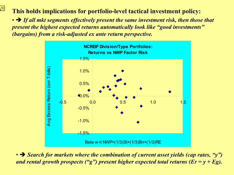
Recall that we see little ability to systematically or rigorousRecall that we see little ability to systematically or rigorously distinguish ly distinguish between the risk and return expectations for different market sebetween the risk and return expectations for different market segments gments withinwithin the asset class (e.g., Denver shopping the asset class (e.g., Denver shopping ctrsctrs vsvs Boston office Boston office bldgsbldgs):):


-1.5%

-1.0%

-0.5%

0.0%

0.5%

1.0%

1.5%

-0.5 0.0 0.5 1.0 1.5


Avg

Exc

ess

Retu

rn (o

vr T

-bills

)

This holds implications for portfolioThis holds implications for portfolio--level tactical investment policy:level tactical investment policy:•• If all If all mktmkt segments effectively present the same investment risk, then thosegments effectively present the same investment risk, then those that se that present the highest expected returns automatically look like “gopresent the highest expected returns automatically look like “good investments” od investments” (bargains) from a risk(bargains) from a risk--adjusted ex ante return perspective.adjusted ex ante return perspective.

•• Search for markets where the combination of current asset yieldSearch for markets where the combination of current asset yields (cap rates, s (cap rates, ““yy””) ) and rental growth prospects (and rental growth prospects (““gg””) present higher expected total returns () present higher expected total returns (ErEr = y + = y + EgEg).).

This is in fact the strategy that most large institutional real estate investment managers and portfolio managers follow. They expend considerable effort digging up information and forecasts about local real estate markets to try to identify these types of opportunities, on both the “buy” and “sell” sides. Market segments with the poorest combination of current asset yields and rental growth prospects are targeted to “sell”, while the opposite are targeted to “buy” (but all within a general minimum required holding period of at least several years, on average, to minimize transaction costs). This is a big part of the “tactical” component of real estate portfolio management. The more “strategic” component involves retaining a substantial degree of diversification across a range of market segments. Sometimes MPT is applied within the real estate asset class to develop such strategic policy guidelines, but more commonly (and more realistically) a much more “heuristic” and common sense based approach to diversification within the asset class is adopted.

Summarizing Chapter 22: Summarizing Chapter 22: Equilibrium Asset Price Equilibrium Asset Price ModellingModelling & Real Estate& Real Estate•• Like the MPT on which it is based, equilibrium asset price Like the MPT on which it is based, equilibrium asset price modellingmodelling (the (the CAPM in particular) has substantial relevance and applicability CAPM in particular) has substantial relevance and applicability to real estate to real estate when applied at the broadwhen applied at the broad--brush brush across asset classesacross asset classes level.level.•• At the property level (At the property level (unleveredunlevered), real estate in general tends to be a low), real estate in general tends to be a low--beta, beta, lowlow--return asset class in equilibrium, but certainly not return asset class in equilibrium, but certainly not risklessriskless, requiring (and , requiring (and providing) some positive risk premium (ex ante).providing) some positive risk premium (ex ante).•• CAPM type models can provide some guidance regarding the relatiCAPM type models can provide some guidance regarding the relative pricing ve pricing of real estate as compared to other asset classes (of real estate as compared to other asset classes (“Should it currently be over“Should it currently be over--weighted or underweighted or under--weighted?”weighted?”), and…), and…•• CAPMCAPM--based riskbased risk--adjusted return measures (such as the adjusted return measures (such as the TreynorTreynor Ratio) may Ratio) may provide a basis for helping to judge the performance of multiprovide a basis for helping to judge the performance of multi--assetasset--class class investment managers (who can allocate across asset classes).investment managers (who can allocate across asset classes).•• WithinWithin the private real estate asset class, the CAPM is less effectivethe private real estate asset class, the CAPM is less effective at at distinguishing between the relative levels of risk among real esdistinguishing between the relative levels of risk among real estate market tate market segments, implying (within the state of current knowledge) a gensegments, implying (within the state of current knowledge) a generally erally flat flat security market linesecurity market line..•• This holds implications for tactical portfolio investment policThis holds implications for tactical portfolio investment policy within the y within the private real estate asset class:private real estate asset class: Search for market segments with a combination Search for market segments with a combination of high asset yields and high rental growth opportunities: Such of high asset yields and high rental growth opportunities: Such apparent apparent ““bargainsbargains”” present favorable riskpresent favorable risk--adjusted ex ante returns.adjusted ex ante returns.

See the Ling-Naranjo article in the Supplemental Reader (and discussion in Chapter 22, section 22.3.3) for a glimpse at some of the cutting edge academic research trying to further develop equilibrium asset price modelling for real estate applications.

chapters 21 & 22 modern portfolio theory equilibrium …€¦ · · 2017-05-10modern...

Documents