chapter2 understanding errors and uncertain ...groups.physics.northwestern.edu/lab/first/errors and...

Chapter 2

Understanding Errors and Uncertain-ties in the Physics Laboratory

2.1 Introduction

We begin with a review of general properties of measurements and how measurements affectwhat we, as scientists, choose to believe and to teach our students. Later we narrow ourscope and dwell on particular strategies for estimating what we know, how well we know it,and what else we might learn from it. We learn to use statistics to distinguish which ideasare consistent with our observations and our data.

2.1.1 Measurements, Observations, and Progress in Physics

Physics, like all natural sciences, is a discipline driven by observation. The concepts andmethodologies that you learn about in your lectures are not taught because they were firstenvisioned by famous people, but because they have been observed always to describe theworld. For these claims to withstand the test of time (and repeated testing in future scientificwork), we must have some idea of how well theory agrees with experiment, or how wellmeasurements agree with each other. Models and theories can be invalidated by conflictingdata; making the decision of whether or not to do so requires understanding how stronglydata and theory agree or disagree. Measurement, observation, and data analysis are keycomponents of physics, equal with theory and conceptualization.

Despite this intimate relationship, the skills and tools for quantifying the quality ofobservations are distinct from those used in studying the theoretical concepts. This briefintroduction to errors and uncertainty represents a summary of key introductory ideas forunderstanding the quality of measurement. Of course, a deeper study of statistics wouldenable a more quantitative background, but the outline here represents what everyone whohas studied physics at the introductory level should know.

Based on this overview of uncertainty, you will perhaps better appreciate how we havecome to trust scientific measurement and analysis above other forms of knowledge acquisition,precisely because we can quantify what we know and how well we know it.

11

CHAPTER 2: UNCERTAINTIES

2.2 Some References

The study of errors and uncertainties is part of the academic field of statistics. The discussionhere is only an introduction to the full subject. Some classic references on the subject oferror analysis in physics are:

• Philip R. Bevington and D. Keith Robinson, Data Reduction and Error Analysis forthe Physical Sciences, McGraw-Hill, 1992.

• John R. Taylor, An Introduction to Error Analysis; The Study of Uncertainties inPhysical Measurements, University Science Books, 1982.

• Glen Cowan, Statistical Data Analysis, Oxford Science Publications, 1998

2.3 The Nature of Error and Uncertainty

Error is the difference between an observation and the true value.

Error = observed value− true value

The “observation” can be a direct measurement or it can be the result of a calculation thatuses measurements; the “true” value might also be a calculated result. Even if we do notknow the true value, its existence defines our “error”; but in this case we will also be unableto determine our error’s numeric value. The goal of many experiments, in fact, is to estimatethe true value of a physical constant using experimental methods. When we do this our errorcannot be known, so we study our apparatus and estimate our error(s) using knowledge ofour measurement uncertainties.

Example: Someone asks you, what is the temperature? You look at the thermometerand see that it is 71◦ F. But, perhaps, the thermometer is mis-calibrated and the actualtemperature is 72◦ F. There is an error of −1◦ F, but you do not know this. What you canfigure out is the reliability of measuring using your thermometer, giving you the uncertaintyof your observation. Perhaps this is not too important for casual conversation about thetemperature, but knowing this uncertainty would make all the difference in deciding if youneed to install a more accurate thermometer for tracking the weather at an airport or forrepeating a chemical reaction exactly during large-scale manufacturing.

Example: Suppose you are measuring the distance between two points using a meterstick but you notice that the ‘zero’ end of the meter stick is very worn. In this case youcan greatly reduce your likely error by sliding the meter stick down so that the ‘10 cm’mark is aligned with the first point. This is a perfectly valid strategy; however, you mustnow subtract 10 cm from the remaining point(s) location(s). A similar strategy applies (inreverse) if your ruler’s zero is not located at the end and you must measure into a corner; inthis case you must add the extra length to your measurement(s).

12


Another common goal of experiments is to try to verify an equation. To do this wealter the apparatus so that the parameters in the equation are different for each “trial”.As an example we might change the mass hanging from a string. If the equation is valid,then the apparatus responds to these variations in the same way that the equation predicts.We then use graphical and/or numerical analysis to check whether the responses from theapparatus (measurements) are consistent with the equation’s predictions. To answer thisquestion we must address the uncertainties in how well we can physically set each variablein our apparatus, how well our apparatus represents the equation, how well our apparatus isisolated from external (i.e. not in our equation) environmental influences, and how well wecan measure our apparatus’ responses. Once again we would prefer to utilize the errors inthese parameters, influences, and measurements but the true values of these errors cannot beknown; they can only be estimated by measuring them and we must accept the uncertaintiesin these measurements as preliminary estimates for the errors.

2.3.1 Sources of Error

No real physical measurement is exactly the same every time it is performed. The uncertaintytells us how closely a second measurement is expected to agree with the first. Errors canarise in several ways, and the uncertainty should help us quantify these errors. In a way theuncertainty provides a convenient ‘yardstick’ we may use to estimate the error.

• Systematic error: Reproducible deviation of an observation that biases the results,arising from procedures, instruments, or ignorance. Each systematic error biasesevery measurement in the same direction, but these directions and amounts vary withdifferent systematic errors.

• Random error: Uncontrollable differences from one trial to another due to environ-ment, equipment, or other issues that reduce the repeatability of an observation. Theymay not actually be random, but deterministic (if you had perfect information): dust,electrical surge, temperature fluctuations, etc. In an ideal experiment, random errorsare minimized for precise results. Random errors are sometimes positive and sometimesnegative; they are sometimes large but are more often small. In a sufficiently largesample of the measurement population, random errors will average out.

Random errors can be estimated from statistical repetition and systematic errors can beestimated from understanding the techniques and instrumentation used in an observation;many systematic errors are identified while investigating disagreement between differentexperiments.

Other contributors to uncertainty are not classified as ‘experimental error’ in the samescientific sense, but still represent difference between measured and ‘true’ values. Thechallenges of estimating these uncertainties are somewhat different.

• Mistake, or ‘illegitimate errors’: This is an error introduced when an experi-menter does something wrong (measures at the wrong time, notes the wrong value).

13


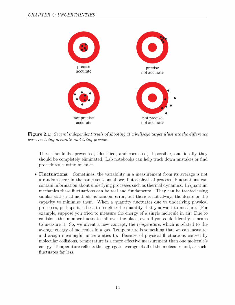
not preciseaccurate

not precisenot accurate

preciseaccurate

precisenot accurate

Figure 2.1: Several independent trials of shooting at a bullseye target illustrate the differencebetween being accurate and being precise.

These should be prevented, identified, and corrected, if possible, and ideally theyshould be completely eliminated. Lab notebooks can help track down mistakes or findprocedures causing mistakes.

• Fluctuations: Sometimes, the variability in a measurement from its average is nota random error in the same sense as above, but a physical process. Fluctuations cancontain information about underlying processes such as thermal dynamics. In quantummechanics these fluctuations can be real and fundamental. They can be treated usingsimilar statistical methods as random error, but there is not always the desire or thecapacity to minimize them. When a quantity fluctuates due to underlying physicalprocesses, perhaps it is best to redefine the quantity that you want to measure. (Forexample, suppose you tried to measure the energy of a single molecule in air. Due tocollisions this number fluctuates all over the place, even if you could identify a meansto measure it. So, we invent a new concept, the temperature, which is related to theaverage energy of molecules in a gas. Temperature is something that we can measure,and assign meaningful uncertainties to. Because of physical fluctuations caused bymolecular collisions, temperature is a more effective measurement than one molecule’senergy. Temperature reflects the aggregate average of all of the molecules and, as such,fluctuates far less.

14


2.3.2 Accuracy vs. Precision

Errors and uncertainties have two independent aspects:

• Accuracy: Accuracy is how closely a measurement comes to the ‘true’ value. Itdescribes how well we eliminate systematic error and mistakes.

• Precision: Precision is how exactly a result is determined without referring to the‘true’ value. It describes how well we suppress random errors and thus how well asequence of measurements of the same physical quantity agree with each other.

It is possible to acquire two precise, but inaccurate, measurements using different instrumentsthat do not agree with each other at all. Or, you can have two accurate, but imprecise,measurements that are very different numerically from each other, but statistically cannotbe distinguished.

2.4 Notation of Uncertainties

There are several ways to write various numbers and uncertainties, but we will describe ourdata using Absolute Uncertainty: The magnitude of the uncertainty of a number in thesame units as the result. We use the symbol δx for the uncertainty in x, and express theresult as x± δx.Example: For an uncertainty δx = 6 cm in a length measurement L of x = 2meters, wewould write L = (2.00± 0.06)m. Note that x and δx have the same number of digits afterthe decimal point. In fact, δx tells us how many digits in x are truly measurable and allowsus to discard the noise; because of this x and δx always have the same number of decimalplaces.

2.5 Estimating Uncertainties

The process of estimating uncertainties requires practice and feedback. Uncertainties arealways due to the measuring tool and to our proficiency with using it.

2.5.1 Level of Uncertainty

How do you actually estimate an uncertainty? First, you must settle on what the quantityδx actually means. If a value is given as x ± δx, what does the range ±δx mean? This iscalled the level of confidence of the results.

Assuming no systematic biases, x− δx < true value < x+ δx 68% of the time. There arevalid reasons to specify tolerances much greater than the statistical uncertainty. For example,

15


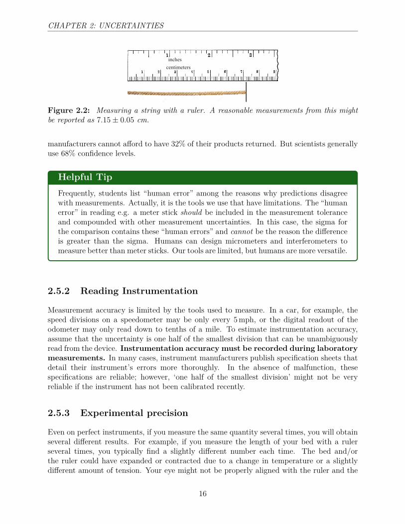
inchescentimeters

Figure 2.2: Measuring a string with a ruler. A reasonable measurements from this mightbe reported as 7.15± 0.05 cm.

manufacturers cannot afford to have 32% of their products returned. But scientists generallyuse 68% confidence levels.

Helpful TipFrequently, students list “human error” among the reasons why predictions disagreewith measurements. Actually, it is the tools we use that have limitations. The “humanerror” in reading e.g. a meter stick should be included in the measurement toleranceand compounded with other measurement uncertainties. In this case, the sigma forthe comparison contains these “human errors” and cannot be the reason the differenceis greater than the sigma. Humans can design micrometers and interferometers tomeasure better than meter sticks. Our tools are limited, but humans are more versatile.

2.5.2 Reading Instrumentation

Measurement accuracy is limited by the tools used to measure. In a car, for example, thespeed divisions on a speedometer may be only every 5mph, or the digital readout of theodometer may only read down to tenths of a mile. To estimate instrumentation accuracy,assume that the uncertainty is one half of the smallest division that can be unambiguouslyread from the device. Instrumentation accuracy must be recorded during laboratorymeasurements. In many cases, instrument manufacturers publish specification sheets thatdetail their instrument’s errors more thoroughly. In the absence of malfunction, thesespecifications are reliable; however, ‘one half of the smallest division’ might not be veryreliable if the instrument has not been calibrated recently.

2.5.3 Experimental precision

Even on perfect instruments, if you measure the same quantity several times, you will obtainseveral different results. For example, if you measure the length of your bed with a rulerseveral times, you typically find a slightly different number each time. The bed and/orthe ruler could have expanded or contracted due to a change in temperature or a slightlydifferent amount of tension. Your eye might not be properly aligned with the ruler and the

16


bed so that parallax varies the measurements. These unavoidable uncertainties are alwayspresent to some degree in an observation. In fact, if you get the same answer every time,you probably need to estimate another decimal place (or even two). Even if you understandtheir origin, the randomness cannot always be controlled. We can use statistical methodsto quantify and to understand these random uncertainties. Our goal in measuring is notto get the same number every time, but rather to acquire the most accurate and precisemeasurements that we can.

2.6 Quantifying Uncertainties

Here we note some mathematical considerations of dealing with random data. These resultsfollow from the central limit theorem in statistics and analysis of the normal distribution.This analysis is beyond the scope of this course; however, the distillation of these studies arethe point of this discussion.

2.6.1 Mean, Standard Deviation, and Standard Error

Statistics are most applicable to very large numbers of samples; however, even 5-10 samplesbenefit from statistical treatment. Statistics greatly reduce the effect of truly random fluctu-ations and this is why we utilize this science to assist us in understanding our observations.But it is still imperative that we closely monitor our apparatus, the environment, and ourprecision for signs of systematic biases that shift the mean.

With only a few samples it is not uncommon(

12N)for all samples to be above (or below)

the distribution’s mean. In these cases the averages that we compute are biased and notthe best representation of the distribution. These samples are also closely grouped so thatthe standard error is misleadingly small. This is why it is important to develop the art ofestimating measurement uncertainties in raw data as a sanity check for such eventualities.

The mean

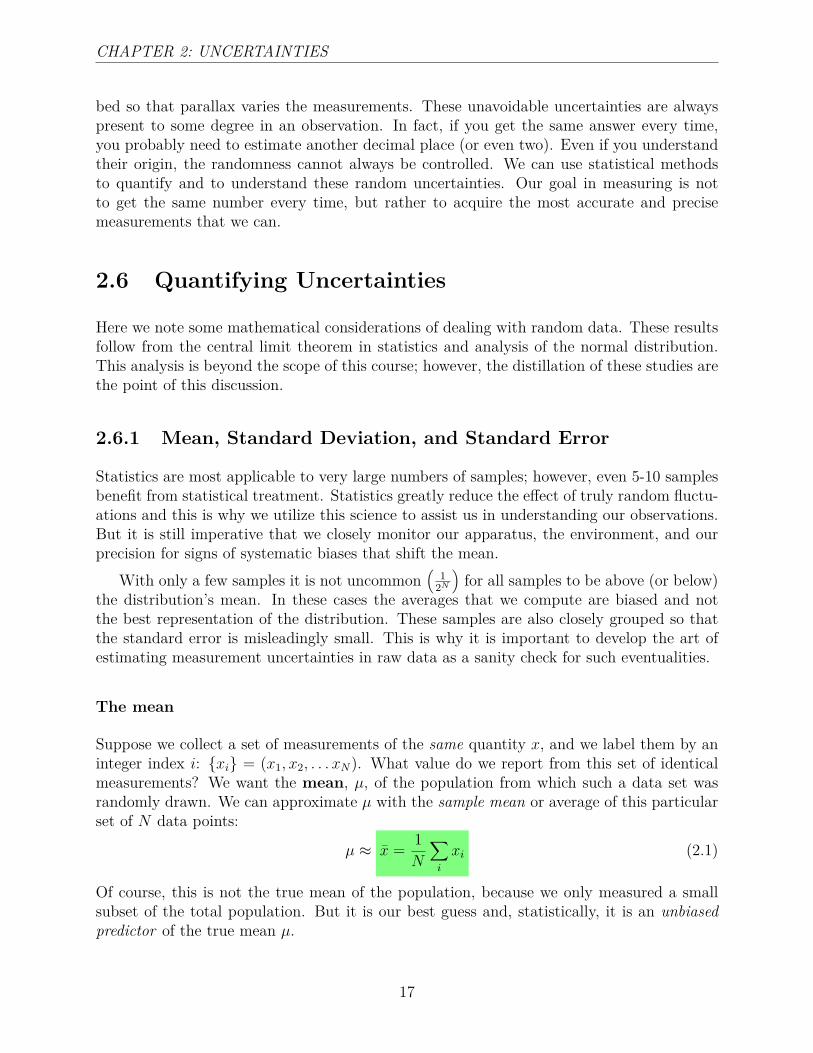
Suppose we collect a set of measurements of the same quantity x, and we label them by aninteger index i: {xi} = (x1, x2, . . . xN). What value do we report from this set of identicalmeasurements? We want the mean, µ, of the population from which such a data set wasrandomly drawn. We can approximate µ with the sample mean or average of this particularset of N data points:

µ ≈ x̄ = 1N

∑i

xi (2.1)

Of course, this is not the true mean of the population, because we only measured a smallsubset of the total population. But it is our best guess and, statistically, it is an unbiasedpredictor of the true mean µ.

17


The standard deviation

How precisely do we know the value of x? To answer this question of statistical uncertaintybased on the data set {xi}, we consider the squared deviations from the sample mean x̄.The sample variance s2

x is the sum of the squared deviations divided by the ‘degrees offreedom’ (DOF). For N measurements the DOF for variance is N − 1. (The origin of theN − 1 is a subtle point in statistics. Ask if you are interested.) The sample standarddeviation, sx, is the square root of the sample variance of the measurements of x.

sx =√∑N

i=1(xi − x̄)2

DOF (2.2)

The sample standard deviation is our best ‘unbiased estimate’ of the true statistical standarddeviation σx of the population from which the measurements were randomly drawn; thus itis what we use for a 68% confidence interval for one measurement (i.e. each of the xi).

The standard error

If we do not care about the standard deviation of one measurement but, rather, how wellwe can rely on a calculated average value, x̄, then we should use the standard error orstandard deviation of the mean sx̄. This is found by dividing the sample standard deviationby√N :

sx̄ = sx√N. (2.3)

If we draw two sets of random samples from the same distribution and compute the twomeans, the two standard deviations, and the two standard errors, then the two means willagree with each other within their standard errors 68% of the time.

2.6.2 Reporting Data

Under normal circumstances, the best estimate of a measured value x predicted from a set ofmeasurements {xi} is given by x = x̄± sx̄ . Statistics depend intimately upon large numbersof samples and none of our experiments will obtain so many samples. Our uncertainties willhave 1-2 significant figures of relevance and the uncertainties tell us how well we know ourmeasurements. Therefore, we will round our uncertainties, δm, to 1-2 significantfigures and then we will round our measurements, m, to the same number ofdecimal places; (3.21± 0.12) cm, (434.2± 1.6)nm, etc.

2.6.3 Error Propagation

One of the more important rules to remember is that the measurements we make have arange of uncertainty so that any calculations using those measurements also must have a

18


commensurate range of uncertainty. After all the result of the calculation will be differentfor each number we should choose even if it is within range of our measurement.

We need to learn how to propagate uncertainty through a calculation that dependson several uncertain quantities. Final results of a calculation clearly depend on theseuncertainties, and it is here where we begin to understand how. Suppose that you havetwo quantities x and y, each with an uncertainty δx and δy, respectively. What is theuncertainty of the quantity x + y or xy? Practically, this is very common in analyzingexperiments and statistical analysis provides the answers disclosed below.

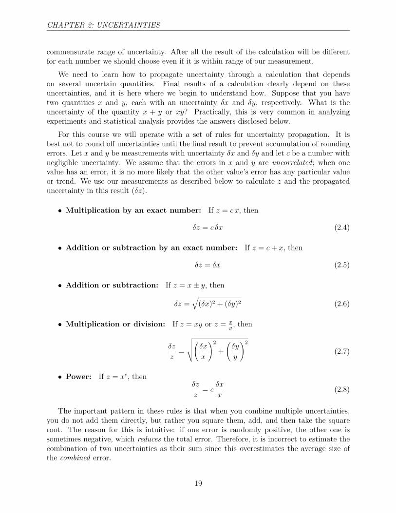
For this course we will operate with a set of rules for uncertainty propagation. It isbest not to round off uncertainties until the final result to prevent accumulation of roundingerrors. Let x and y be measurements with uncertainty δx and δy and let c be a number withnegligible uncertainty. We assume that the errors in x and y are uncorrelated; when onevalue has an error, it is no more likely that the other value’s error has any particular valueor trend. We use our measurements as described below to calculate z and the propagateduncertainty in this result (δz).

• Multiplication by an exact number: If z = c x, then

δz = c δx (2.4)

• Addition or subtraction by an exact number: If z = c+ x, then

δz = δx (2.5)

• Addition or subtraction: If z = x± y, then

δz =√

(δx)2 + (δy)2 (2.6)

• Multiplication or division: If z = xy or z = xy, then

δz

z=

√√√√(δxx

)2

+(δy

y

)2

(2.7)

• Power: If z = xc, thenδz

z= c

δx

x(2.8)

The important pattern in these rules is that when you combine multiple uncertainties,you do not add them directly, but rather you square them, add, and then take the squareroot. The reason for this is intuitive: if one error is randomly positive, the other one issometimes negative, which reduces the total error. Therefore, it is incorrect to estimate thecombination of two uncertainties as their sum since this overestimates the average size ofthe combined error.

19


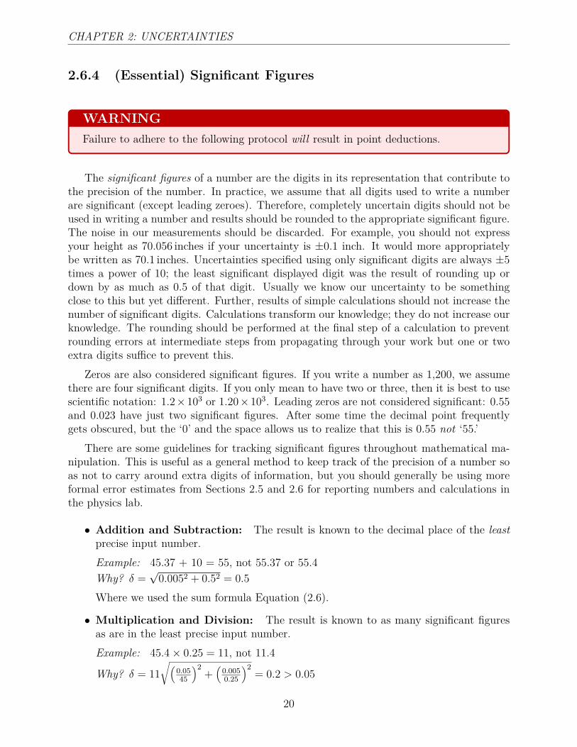
2.6.4 (Essential) Significant Figures

WARNINGFailure to adhere to the following protocol will result in point deductions.

The significant figures of a number are the digits in its representation that contribute tothe precision of the number. In practice, we assume that all digits used to write a numberare significant (except leading zeroes). Therefore, completely uncertain digits should not beused in writing a number and results should be rounded to the appropriate significant figure.The noise in our measurements should be discarded. For example, you should not expressyour height as 70.056 inches if your uncertainty is ±0.1 inch. It would more appropriatelybe written as 70.1 inches. Uncertainties specified using only significant digits are always ±5times a power of 10; the least significant displayed digit was the result of rounding up ordown by as much as 0.5 of that digit. Usually we know our uncertainty to be somethingclose to this but yet different. Further, results of simple calculations should not increase thenumber of significant digits. Calculations transform our knowledge; they do not increase ourknowledge. The rounding should be performed at the final step of a calculation to preventrounding errors at intermediate steps from propagating through your work but one or twoextra digits suffice to prevent this.

Zeros are also considered significant figures. If you write a number as 1,200, we assumethere are four significant digits. If you only mean to have two or three, then it is best to usescientific notation: 1.2×103 or 1.20×103. Leading zeros are not considered significant: 0.55and 0.023 have just two significant figures. After some time the decimal point frequentlygets obscured, but the ‘0’ and the space allows us to realize that this is 0.55 not ‘55.’

There are some guidelines for tracking significant figures throughout mathematical ma-nipulation. This is useful as a general method to keep track of the precision of a number soas not to carry around extra digits of information, but you should generally be using moreformal error estimates from Sections 2.5 and 2.6 for reporting numbers and calculations inthe physics lab.

• Addition and Subtraction: The result is known to the decimal place of the leastprecise input number.Example: 45.37 + 10 = 55, not 55.37 or 55.4Why? δ =

√0.0052 + 0.52 = 0.5

Where we used the sum formula Equation (2.6).

• Multiplication and Division: The result is known to as many significant figuresas are in the least precise input number.Example: 45.4× 0.25 = 11, not 11.4

Why? δ = 11√(

0.0545

)2+(

0.0050.25

)2= 0.2 > 0.05

20


Where we used the product formula Equation (2.7).

Example: If you measure a value on a two-digit digital meter to be 1.0 and anothervalue to be 3.0, it is incorrect to say that the ratio of these measurements is 0.3333333, evenif that is what your calculator screen shows you. The two values are measurements; they arenot exact numbers with infinite precision. Since they each have two significant digits, thecorrect number to write down is 0.33. If this is an intermediate result, then 0.333 or 0.3333are preferred, but the final result must have two significant digits.

For this lab, you should use proper significant figures for all reported numbers includingthose in your notebook. We will generally follow a rule for significant figures in reportednumbers: calculate your uncertainty to two significant figures, if possible, usingthe approach in Sections 2.5 and 2.6, and then use the same level of precision inthe reported error and measurement. This is a rough guideline, and there are timeswhen it is more appropriate to report more or fewer digits in the uncertainty. However, it isalways true that the result must be rounded to the same decimal place as the uncertainty.The uncertainty tells us how well we know our measurement.

2.7 How to Plot Data in the Lab

Plotting data correctly in physics lab is somewhat more involved than just drawing points ongraph paper. First, you must choose appropriate axes and scales. The axes must be scaledso that the data points are spread out from one side of the page to the other. Axes mustalways be labeled with physical quantity plotted and the data’s units. Then, plot yourdata points on the graph. Ordinarily, you must add error bars to your data points, butwe forgo this requirement in the introductory labs. Often, we only draw error bars in thevertical direction, but there are cases where it is appropriate to have both horizontal andvertical error bars. In this course, we would use one standard deviation (standard error ifappropriate for the data point) for the error bar. This means that 68% of the time the ‘true’value should fall within the error bar range.

Do not connect your data points by line segments. Rather, fit your data points to amodel (often a straight line), and then add the best-fit model curve to the figure. The line,representing your theoretical model, is the best fit to the data collected in the experiment.Because the error bars represent just one standard deviation, it is fairly common for a datapoint to fall more than an error bar away from the fit line. This is OK! Your error barsare probably too large if the line goes through all of them! Since 32% of your data pointsare more than 1σ away from the model curve, you can use this fact to practice choosingappropriate uncertainties in your raw data.

Some of the fitting parameters are usually important to our experiment as measuredvalues. These measured parameters and other observations help us determine whether thefitting model agrees or disagrees with our data. If they agree, then some of the fittingparameters might yield measurements of physical constants.

21


2.8 Fitting Data (Optional)

Fully understanding this section is not required for Physics 136. You will use least-squaresfitting in the laboratory, but we will not discuss the mathematical justifications of curve fittingdata. Potential physics and science majors are encouraged to internalize this material; it willbecome an increasingly important topic in upper division laboratory courses and research andit will be revisited in greater detail.

In experiments one must often test whether a theory describes a set of observations.This is a statistical question, and the uncertainties in data must be taken into account tocompare theory and data correctly. In addition, the process of ‘curve fitting’ might provideestimates of parameters in the model and the uncertainty in these parameter estimations.These parameters tailor the model to your particular set of data and to the apparatus thatproduced the data.

Curve fitting is intimately tied to error analysis through statistics, although the math-ematical basis for the procedure is beyond the scope of this introductory course. Thisfinal section outlines the concepts of curve fitting and determining the ‘goodness of fit’.Understanding these concepts will provide deeper insight into experimental science and thetesting of theoretical models. We will use curve fitting in the lab, but a full derivationand statistical justification for the process will not be provided in this course.The references in Section 2.2, Wikipedia, advanced lab courses, or statistics textbooks willall provide a more detailed explanation of data fitting.

2.8.1 Least-Squares and Chi-Squared Curve Fitting

Usually data follows a mathematical model and the model has adjustable parameters (slope,y-intercept, etc.) that can be optimized to make the model fit the data better. To do this wecompute the vertical distance between each data point and the model curve, we add togetherall of these distances, and then we adjust all of the parameters to minimize this sum. Thisstrategy is the “least squares” algorithm for fitting curves.

Scientific curve fits benefit from giving more precise data points a higher weight thanpoints that are less well-known. This strategy is “chi squared” curve fitting. These algorithmsmay be researched readily on the internet.

2.9 Strategy for Testing a Model

2.9.1 A Comparison of Measurements

If we have two independent measurements, X1 = x1 ± δx1 and X2 = x2 ± δx2, of the samephysical quantity and having the same physical units, then we will conclude that they agreeif the smaller plus its δ overlaps with the larger minus its δ.

22


A disagreement could mean that the data contradicts the theory being tested, butit could also just mean that one or more assumptions are not valid for the experiment;perhaps we should revisit these. Disagreement could mean that we have underestimatedour errors (or even have overlooked some altogether); closer study of this possibility will beneeded. Disagreement could just mean that this one time the improbable happened. Thesepossibilities should specifically be mentioned in your Analysis according to which is mostlikely, but further investigation will await another publication.

Helpful TipOne illegitimate source of disagreement that plagues students far too often is simplemath mistakes. When your data doesn’t agree and it isn’t pretty obvious why, hideyour previous work and repeat your calculations very carefully to make sure you getthe same answer twice. If not, investigate where the two calculations began to differ.

23

chapter2 understanding errors and uncertain ...groups.physics.northwestern.edu/lab/first/errors and...

Documents