Chapter VI

Numerical Methods

VI.1 Development of an Open-Source CFD Solver

One of the general goals of computational fluid dynamics (CFD) is to

accurately solve the Navier-Stokes equations. For incompressible flow, these equa-

tions can be written in a generalized form:

@ui

@t+

@ujui

@xj� ⌫

@2ui

@x2j

+@p

@xi= ��1iPx(x, t) + fi(�).

@uj

@xj= 0,

To solve this problem numerically, the continuous flow field must be ap-

proximated on a discrete set of points in space. Further, the resulting approximate

equation on this finite set of points must be advanced in time using discrete time

steps. To minimize the expense of the computation, one desires to use as few

spatial points as possible with large time steps while maintaining the accuracy (in

both space and time) and stability of the simulation. With a particular spatial dis-

cretization, some terms of the governing equation will impose a more stringent time

step limitation than other terms. Generally, the most restrictive terms should be

treated implicitly to increase numerical stability, while other less restrictive terms

may be taken explicitly. These issues guide the choice of spatial and temporal

discretizations of the current problem, which are discussed in detail below.

150

151

Diablo is an open-source CFD solver designed by Professor Thomas Bew-

ley. The channel flow solver, scalar advection, and geophysical forcing terms were

written by the author with guidance from Professors Bewley and Sarkar. Extra

features such as the inclusion of a Darcy force for porous media and immersed

obstacles are being added by other students at UCSD. The goal of Diablo is to

provide an e�cient and easy to use solver for incompressible, three-dimesional tur-

bulent flows in simple geometries. The code has been designed to allow an arbitrary

choice of periodic directions, although only those with two or three periodic direc-

tions are fully functional at this time. When a given direction is made periodic,

all derivatives in that direction are computed in Fourier space. This improves the

accuracy of the algorithm and minimizes the numerical dissipation.

Time stepping in Diablo uses a combination of the explicit third-order

Runge-Kutta and the implicit Crank Nicolson schemes. In order for the time-

stepping of di↵usion problems to be stable when using the Runge-Kutta or other

explicit methods, the condition of stability requires that the di↵usion number

defined as D = ⌫�t/�x2 be less than some constant. For a given grid spacing this

places a condition on the size of �t. Since the grid spacing must scale inversely

with the Reynolds number this can place a severe limitation on the allowable time-

step. The Crank-Nicolson scheme, however, is unconditionally stable for the pure

di↵usion problem. For wall bounded flows, the minimum grid spacing generally

occurs in the wall-bounded direction and near the wall which motivates the choice

of treating the di↵usion terms with Crank-Nicolson.

The Runge-Kutta method evaluates the right hand side multiple times for

each timestep and uses these “trial” steps to improve the accuracy of the scheme.

See Press et al. [90] or Bewley [11] for an introduction to the method. Since RAM

may be a limiting factor for the problem size in some applications, the low-storage

Runge-Kutta-Wray algorithm is used here. The algorithm can be written [11]

k1 = f(yn, tn), (VI.1)

k2 = f(yn + �1hk1, tn + ↵1h), (VI.2)

152

k3 = f(yn + �2hk1 + �3hk2, tn + ↵2h), (VI.3)

yn+1 = yn + h(�1k1 + �2k2 + �3k3), (VI.4)

where

�1 = 8/15, �2 = 1/4, �3 = 5/12,

↵1 = 8/15, ↵2 = 2/3,

�1 = 1/4, �2 = 0, �3 = 3/4.

Although there are four equations, when the algorithm is ordered carefully only

two storage variables are needed.

In order to ensure that the velocity field is divergence free as required by

mass conservation under the Boussinesq approximation, the fractional step method

is used. First, at each Runge-Kutta substep (j=1,2,3), time-marching produces an

intermediate velocity field uij that may not be solenoidal. The second step of the

fractional step method then uses the pressure gradient to ensure that the velocity

is divergence free. If the corrected velocity field is denoted uji :

uji = ui

j � hj@�

@xi, (VI.5)

where � = pj+1 � pj is the pressure adjustment between successive Runge-Kutta

substeps and hj is proportional to the timestep and for the RKW3 scheme is:

h1 =8

15�t (VI.6)

h2 =2

15�t

h3 =5

15�t.

Taking the divergence of Eq. VI.5 gives a Poisson equation for � involving only

the known uij since, by definition, uj

i is divergence free:

r2� =1

hjr · ui

j. (VI.7)

When this equation is solved in Fourier space with second order finite di↵erences

in one direction, we obtain a tridiagonal system of equations for the discrete �.

153

After solving the Poisson equation, � is used to update the pressure and the velocity

through Eq. VI.5. In order to ensure that he discrete continuity equation is satisfied

at the walls, homogeneous Neumann boundary conditions are applied to �. Notice

that with these boundary condtions, the value of � is undetermined by an additive

constant. In order to make the Poisson equation well-posed we arbitrarily set the

mean pressure at the lower boundary to be zero.

The computational domain is discretized in the horizontal directions with

a uniform grid-spacing and co-located variables, allowing these directions to be

transformed e�ciently to and from Fourier space. The discrete Fourier transforms

are calculated using the freely available FFTW software (see www.↵tw.org or Frigo

and Johnson [34]). This software is one of the fastest publicly available discrete

Fourier transform algorithms. While some machine-specific algorithms may be

slightly faster, the advantage of FFTW is that it can be used on a variety of

computer architectures, allowing Diablo to be e�cient and portable. The speed of

FFTW is achieved by creating an adaptive plan utilizing a combination of FFT

solvers and that determined at runtime and is optimized for the problem size and

local architecture [34].

The Fourier transform of a discrete field fj defined on the grid j = 1...N

will be denoted by fk where the discrete wavenumbers are k = �N/2...0...N/2.

Since we are interested in real functions in physical space, when f is real fk = f ⇤�k

where ⇤ denotes the complex conjugate. Since f0 is real, we only need to keep

1...N/2 complex numbers. The Nyquist frequency, k = ±N/2 presents problems

when considering an odd number of spectral derivatives, so the coe�cients fN/2

and f�N/2 are set to zero [11]. Other high wavenumbers also present a problem

in spectral methods. The nonlinear term in the momentum can transfer energy

from low to high-wavenumers. If two relatively large wavenumber modes interact

through the nonlinear term, they can produce energy to wavenumbers larger than

the Nyquist [11]. The resulting wavenumbers, |k| > N/2 cannot be represented

with a discrete Fourier series and will be aliased to lower wavenumbers. This

154

occurs since the k Fourier mode and the k + mN mode look the same where m

is a positive or negative integer [19]. It is therefore possible for high wavenumers

to feed spurious energy to low wavenumber modes, contaminating the solution. In

order to remedy this, the Orszag 2/3 de-aliasing method is used (see Canuto et al.

[19] for a description). In Diablo, this is done by zeroing all Fourier modes with

wavenumbers k > N/3 before transforming to physical space.

Evaluation of the nonlinear term in the Navier-Stokes equations in a spec-

tral code is not straightforward. For the terms that involve a horizontal derivative,

we would like to evaluate the derivate in Fourier space to get spectral accuracy.

However, since these terms involve a product, evaluating it in Fourier space would

require computing a discrete convolution sum which requires O(N2) operations

where N is the number of gridpoints in one direction. For large problems, this will

become very computationally costly. Instead, we use the so-called pseudo-spectral

method where the nonlinear term is first written in conservation form:

@

@xj(uiuj). (VI.8)

The product in parentheses is computed in physical space, requiring O(N) opera-

tions. This is then transformed into Fourier space requiring O(N log(N)) operations

using the FFT algorithm, and the derivatives are taken in Fourier space, requiring

an additional O(N) operations. This method of computing the nonlinear term is

then O(N log(N)) instead of O(N2).

G =

G = 0 1 2

1 2 3

j-1 j j+1

j-1 j j+1

N+1N-1 N

N N+1N-1

1/2

Figure VI.1: Grid layout of Diablo in the wall-normal directions. The wall-normal

velocity is stored at G points (open circles), all other variables are stored at G1/2

points (closed circles).

In the wall-bounded finite di↵erence directions, Diablo uses a staggered

155

grid with vertical velocity located at “G” nodes and the horizontal velocity, pres-

sure, and scalars defined at “G1/2” nodes, see figure VI.1. Grid stretching is used

in the wall-bounded directions in order to resolve small-scale turbulence near the

wall. The G1/2 cells are located exactly halfway between neighboring G points.

The staggering is done so that neighboring pressure values are coupled. If central

finite di↵erences were used on a collocated grid, neighboring pressure values would

be coupled only through the viscous term, and so for large Reynolds numbers oscil-

latory solutions may arise [32]. The location of the walls (marked by cross-hatching

in Figure VI.1) are chosen to coincide with horizontal velocity points. Interpola-

tion from the G grid to the G1/2 grid is then accomplished by taking the average

of neighboring values which is second-order accurate. In order to interpolate a

quantity f from the G1/2 to the G grid with second order accuracy, the following

formula is used:

f(Gj1/2) =

1

2�Gj(�Gj�1

1/2 f(Gj1/2) + �Gj

1/2f(Gj�11/2 )). (VI.9)

This equation is not always used for interpolation, and is substituted for less ac-

curate interpolation schemes where necessary to ensure discrete mass, momentum,

and energy conservation as derived by Bewley [10].

In the finite di↵erence directions, boundary conditions are applied using

ghost cells as depicted by gray circles in Figure VI.1. The boundary conditions

can be either Neumann or Dirichlet with the gradient or boundary value specified,

respectively. Since a staggered grid is used, the boundary conditions are not always

applied exactly at the wall locations, but it is ensured that the discrete conservation

properties are satisfied. Since the grid spacing near the wall is small, this should not

significantly a↵ect the results. When Neumann boundary conditions are specified

for the horizontal velocity or the scalars, the value of the ghost cell at G1/2 = 0 and

G1/2 = N+1 is set so that the wall-normal derivative at G = 1 and G = N+1 is the

specified value. Since the wall-normal velocity is o↵set from the wall, its gradient

can easily be specified exactly at the wall. When Dirichlet boundary conditions

are used, the horizontal velocity and scalars are prescribed at the wall locations,

156

while the wall-normal velocity is specified at the G = 2 and G = N points.

In addition to solving the momentum equations, Diablo has the capacity

for timestepping the scalar advection-di↵usion equation. Any number of scalars

can be considered and memory is allocated accordingly. The timestepping for the

scalar equations is done using the same scheme as the momentum equations. Each

scalar is associated with a unique Prandtl and Richardson number, enabling the

consideration of multiple active scalars such as temperature and salinity or passive

scalars to simulate a dye release. The updating of the scalars and velocity is o↵set

so that the scalars at the k+1 step are found using the velocity at the k step, then

the velocity is updated with the buoyancy term evaluated at k + 1. The scalars

coincide with the horizontal velocity points on the staggered grid.

In order to simulate model problems of interest for geophysical applica-

tions, additional terms are included to account for a rotating coordinate frame.

One term, the centripetal acceleration, is conservative and can be expressed as the

gradient of a potential and absorbed into the definition of the pressure. The second

term, the Coriolis acceleration represents a new term in the equations of motion.

For convenience, a background pressure gradient used to force the flow is written

in terms of a geostrophic wind, UG, and included in the Coriolis term. The x-axis

is chosen to be aligned with the geostrophic wind, not necessarily in the east-west

direction. When placed on the right hand side of the momentum equations, the

Coriolis term is:

(�cos(�)sin(�)

sin(�)w + v)i

(cos(�)cos(�)

sin(�)w � u + UG)j (VI.10)

(�cos(�)cos(�)

sin(�)v +

cos(�)sin(�)

sin(�)(u� UG))k.

In deriving this term, we have not assumed that the rotational vector is aligned with

the vertical direction as is done in many ocean models (and called the ‘traditional

approximation’). Instead, � is the latitude, and � is the direction made between

the geostrophic velocity (and the x-axis) and the northward direction.

157

VI.2 Large Eddy Simulation

A direct numerical simulation (DNS) involves solving the Navier-Stokes

equations with specified initial and boundary conditions where the viscosity and

di↵usivity are the molecular values. In order to guarantee accuracy, a DNS must

resolve nearly all scales of motion. The smallest scale that a turbulent eddy can

take before being arrested by viscosity is estimated by the Kolmogorov scale, ⌘

defined as:

⌘ = (⌫3

✏)1/4. (VI.11)

An estimate of the range of scales that must be considered by a DNS can be

obtained by dividing the Kolmogorov scale by the scale of the largest eddies, h.

⌘

h= ⌫3/4✏�1/4h�1 = Re�3/4

o (h✏

U3o

)�1/4, (VI.12)

where Reo = Uoh/⌫, and Uo is the velocity scale associated with the largest scale

motions. The last term in parentheses is the dissipation normalized by the large

scale velocity and length. According to Kolmogorov’s hypothesis, dissipation is

driven by the large scales of motion, independent of viscosity, which implies that

this last term should be independent of Reynolds number. Since a DNS must

resolve the all scales of motion, the number of gridpoints needed in each direction

will scale with h/⌘ which we see from Eq. VI.12 is O(Re3/4o ). The total number of

gridpoints for a three-dimensional simulation will scale with Re9/4o , so a doubling

of the outer Reynolds number requires nearly a five-fold increase in the number

of points used. This requirement is made even more severe since the size of the

timestep that is taken must decrease with the gridspacing, and it can be shown[89]

that the total computational cost scales with Re3o.

Most of the energy in a turbulent flow is contained in the very largest

scales of motion. This is illustrated in Figure VI.2 which shows the one dimensional

velocity spectra from the DNS of turbulent channel flow of Moser et al. [71] at

Re⌧ = 590 taken at a height of z+ = 298. The panel on the left of Figure VI.2

shows the spectra as they are traditionally plotted with logarithmic axes with

158

100 101 10210-7

10-6

10-5

10-4

10-3

10-2

10-1

100

kx

0 50 100 150 2000

0.05

0.1

0.15

0.2

0.25

0.3

0.35

0.4

0.45

0.5

kx

EuuEww

Evvk-5/3

EuuEww

Evv

Figure VI.2: One-dimensional energy spectra for turbulent channel flow at Re⌧ =

590 at z+ = 298 from the data of Moser et al. [71]

the Kolmogorov inertial subrange model spectrum for reference. The panel on

the right shows the same spectra on linear axes. It is clear that most of the

wavenumbers considered by the DNS carried a very small amount of energy. This

does not imply that these scales are not important to the simulations since they

play an important role in the turbulent energy cascade. Still this gives hope that

an adequate representation of the flow may be obtained by directly solving for the

velocity by resolving only the low wavenumbers.

A large eddy simulation (LES) explicitly solves the largest scales of motion

and models the influence of the smaller scales. Specifically, the equations of motion

are filtered in space; when the incompressible, Boussinesq form is used we get:

@ui

@t+

@ujui

@xj= � @p0

@xi�Ri⌧⇢0k +

1

Re⌧

@

@xj

@ui

@xj� @⌧ij

@xj, (VI.13)

159

@⇢

@t+

@uj⇢

@xj=

1

Re⌧Pr

@

@xj

@⇢

@xj� @�j

@xj, (VI.14)

r · u = 0, (VI.15)

where ui denotes the filtered velocity field. The last terms in Eqns. VI.13 and VI.14

represent the a↵ect of the sub-filter scales on the filtered velocity and density. Since

the LES solves only for the filtered velocity, the sub-filter contributions must be

modeled. The residual stress tensor as it appears in equation VI.13 is then: [89]

⌧ij = uiuj � uiuj. (VI.16)

There are many possible choices of models for the sub-filter momentum

stress and buoyancy flux. Here we chose to implement the dynamic Smagorinsky

method with an optional scale-similar part. In the dynamic model, first proposed

by Germano et al. [40], the deviatoric part of the sub-filter stress and buoyancy

flux are written:

⌧ij = �2CM �2 |S|Sij, �i = �C⇢�

2|S| @⇢

@xi, (VI.17)

where � is the filter width, Sij is the resolved rate of strain tensor, and CM and

C⇢ are the dynamic coe�cients that will be set using the dynamic procedure. The

subgrid-scale eddy viscosity is then given by:

⌫sgs = CM�2|S|.

The dynamic coe�cients, CM and C⇢ are determined by applying a test filter to the

LES filtered field. · will denote a field that has been filtered first by the LES filter

and subsequently by the test filter. The scales between the LES and test filter

widths are used to estimate the dynamic coe�cients. Specifically, the dynamic

procedure is:

CM = �1

2

< LijMij >

< MijMij >, (VI.18)

where

Lij = duiuj � bui buj, (VI.19)

160

Mij = b�2c|S|cSij �

\�

2|S|Sij. (VI.20)

The dynamic coe�cient for the sub-filter buoyancy flux is determined in a similar

way:

C⇢ = �1

2

< LiMi >

< MjMj >, (VI.21)

where now

Li = c⇢ui � b⇢bui, Mi = b�2c|S|

d@⇢

@xi��

2 \|S| @⇢

@xi. (VI.22)

Since the dynamic model estimates the sub-filter stress and buoyancy flux

by applying a second ‘test’ filter, the choice of the filter width is the only tunable

parameter in the dynamic model. Here, the test filter can be applied in either

physical or Fourier space. Unless otherwise noted, all applications described here

will apply a filter based on an explict five-point trapezoidal rule. The ratio of the

LES to grid filter widths is taken to be �/�g = 3 which is consistent with the

2/3 de-aliasing that is applied in Fourier space. The ratio of the test to LES filter

is taken to be �/� = 4. It is our experience that �/� = 2, the common choice

for finite di↵erence codes, is not the optimal choice here. Unlike when a filter

is applied in Fourier space, the test filter used here does not have a well-defined

width, and the specified width was found to be optimal based on trial and error.

Although the grid size and the LES filter width are not equal, the terms sub-filter

and sub-grid scale will be used interchangeably to refer to scales unresolved by the

LES.

One advantage of the dynamic model is that it contains few adjustable

parameters and can be used in a variety of flow regimes. For example, for wall-

bounded flows the dynamic coe�cient adjusts so that the length scale associated

with the Smagorinsky coe�cient and the filter width, l = (CM�2)1/2 decreases

near the wall without the use of a prescribed damping function [86]. Piomelli and

Liu [88] considered rotating channel flow and found that the dynamic model LES

performed well compared to a DNS. The dynamic model (with a scale-similar part

to be described below) has been used successfully in many previous studies includ-

161

ing lid-driven cavity flow [116], stratified channel flow [3] [110], and a rotating,

tidally-driven boundary layer [92].

Rig

Pr sgs

0.25 0.5 0.75 10

2

4

6

8

10

12

14

Figure VI.3: Subgrid turbulent Prandtl number and gradient Richardson number

from Armenio and Sarkar[3]

For stratified flow, Armenio and Sarkar [3] found that although strati-

fication is not explicitly represented in the LES model, the dynamic coe�cient

adjusted in a reasonable manner. For example, Figure VI.3 shows that the sub-

grid turbulent Prandtl number increased with the gradient Richardson number in

their simulations of stratified channel flow. While the exact dependence of the

turbulent Prandtl number on the gradient Richardson number is problem specific,

many previous studies show a positive correlation. Figure VI.4 shows the depen-

dence for a variety of numerical studies, field data, and proposed models including

results of the stratified open channel flow presented earlier. While the data varies

significantly, each study shows an increase in the turbulent Prandtl number with

gradient Richardson number, a feature that is automatically picked up by the

dynamic Smagorinsky model.

The primary disadvantage of the dynamic model is the computational

cost. The algorithm that has been written for Diablo seeks to minimize the compu-

162

0 0.5 1 1.5 2 2.5 30

1

2

3

4

5

6

7

8

9

10

Rig

PrT

Armenio and Sarkar, C1Armenio and Sarkar, C4Jacobitz and Sarkar DNSTaylor et al. (2005)Monti et al. (2002) FieldJoseph et al. (2004) Jet DNSJoseph et al. (2004) Jet DNSKaltenbach et al. (1994) LESSchumann and Gerz (1995)ModelTjernstrom (1993) ModelKim and Mahrt (1992) ModelPacanowski and Philander (1981) Model

Figure VI.4: Dependence of the turbulent Prandtl number on the gradient Richard-

son number

tational cost, sometimes at the expense of added memory allocation. For example,

Sij, |S|, and ui are computed at every point in space and placed in storage arrays

at start of the dynamic procedure since each are needed in multiple places in the

algorithm. Since a LES with the dynamic model is significantly more expensive

than a DNS for the same number of gridpoints, it is unlikely that available mem-

ory will be a limiting factor for a LES. A measure of the computational load can

be estimated by considering the number of FFT calls, the most expensive oper-

ation in the algorithm. In an unstratified DNS, Diablo requires 14 calls to the

FFT algorithm (including both forward and inverse transforms) for each Runge-

Kutta substep. The dynamic procedure adds 12 FFT calls, which are requried

to transform the six unique components of the Sij tensor to physical space where

products are computed and to transform the sub-filter stress-tensor to Fourier

space since derivatives in the horizontal directions are needed for the contribution

to the momentum equations. For an unstratified DNS, Diablo requires 14 three-

163

dimensional storage arrays. The dynamic mixed subgrid-scale model used for the

LES more than doubles the memory requirement by requiring an additional 19

three-dimensional storage arrays.

In the above equations for the dynamic model coe�cients, < · > denotes

an averaging operator. This was introduced by Germano et al. [40] in a channel

flow application where the average was taken over the planes parallel to the walls.

Since it is possible for Mij to be zero, Germano introduces the averaging operator to

keep CM well-conditioned. When CM is positive, the model is purely dissipative;

that is the subgrid-scale model acts as a sink for the resolved turbulent kinetic

energy. If CM were less than zero than the opposite would be true and energy

would be transferred from the subgrid to the resolved scale motions, a process

known as backscatter. By considering the interactions of various Fourier modes

through the nonlinear term in the momentum equations, it can be shown that

backscatter is possible and may sometimes be expected locally in physical space

[89]. It is unlikely that the dynamic coe�cient would remain less than zero after

taking a plane average, but local averaging techniques have been proposed such

as the Lagrangian averaging method of Meneveau et al. [69]. As suggested by

Germano et al. [40] when averaged locally, CM can take on negative values and

represent backscatter. In practice, however, it is found that negative values of CM

lead to numerical instabilities, and in practice when this occurs CM is set to zero

[68]. In this study, since all problems of interest are statistically homogeneous in

the horizontal directions, CM and C⇢ are always averaged over horizontal planes

and set to zero if they ever become negative.

The assumption that the subgrid stress tensor is aligned with the strain

rate tensor and that the subgrid is purely dissipative can be relaxed by including

an addition term in the subgrid model. Bardina et al. [6] proposed a scale-similar

model, in which it is assumed that the unresolved stress is proportional to the sub

test-filter stress:

⌧ij = duiuj � bui buj. (VI.23)

164

Since ui is known, we can then compute the sub test-filter stress directly. This

model does allow energy transfer from the unresolved to the resolved scales, but it

is generally not dissipative enough and Bardina [6] proposed combining it with an

eddy viscosity model. Zang et al. [116] was the first to combine the scale similar

model with a dynamic eddy viscosity model to form the so-called dynamic mixed

model (DMM). This model has been implemented in Diablo and it has been shown

to perform very well in a variety of situations [68]. With the DMM, the subgrid

scale stress tensor is:

⌧ij = (duiuj � uiuj)� 2CM�2|S|Sij, (VI.24)

and the equation for the dynamic coe�cient has an extra term:

CM = �1

2

< LijMij > � < NijMij >

< MijMij >, (VI.25)

where

Nij = (dbui buj �

bbuibbuj)� (duiuj � duiuj). (VI.26)

Note that the scale-similar part is considered only for the momentum equation; the

subgrid buoyancy flux is modeled as in Eq. VI.21 with a dynamic eddy viscosity

model.

VI.3 Open Boundary Conditions

In order to approximate an unbounded domain in the vertical, an open

boundary condition is employed. This is accomplished through a combination of

a Rayleigh damping or ‘sponge’ layer and a radiation condition. An introduction

to both types of boundary conditions can be found in Durran ??.

The concept behind the sponge layer is simple: in a region at the top of the

computational domain, the velocity and scalar fields are relaxed towards a specified

background state. Sponge layers can be very e↵ective at eliminating reflections if

165

02

46

0

1

2

3

4

5

6

(a)

02

46

0

1

2

3

4

5

6

(b)

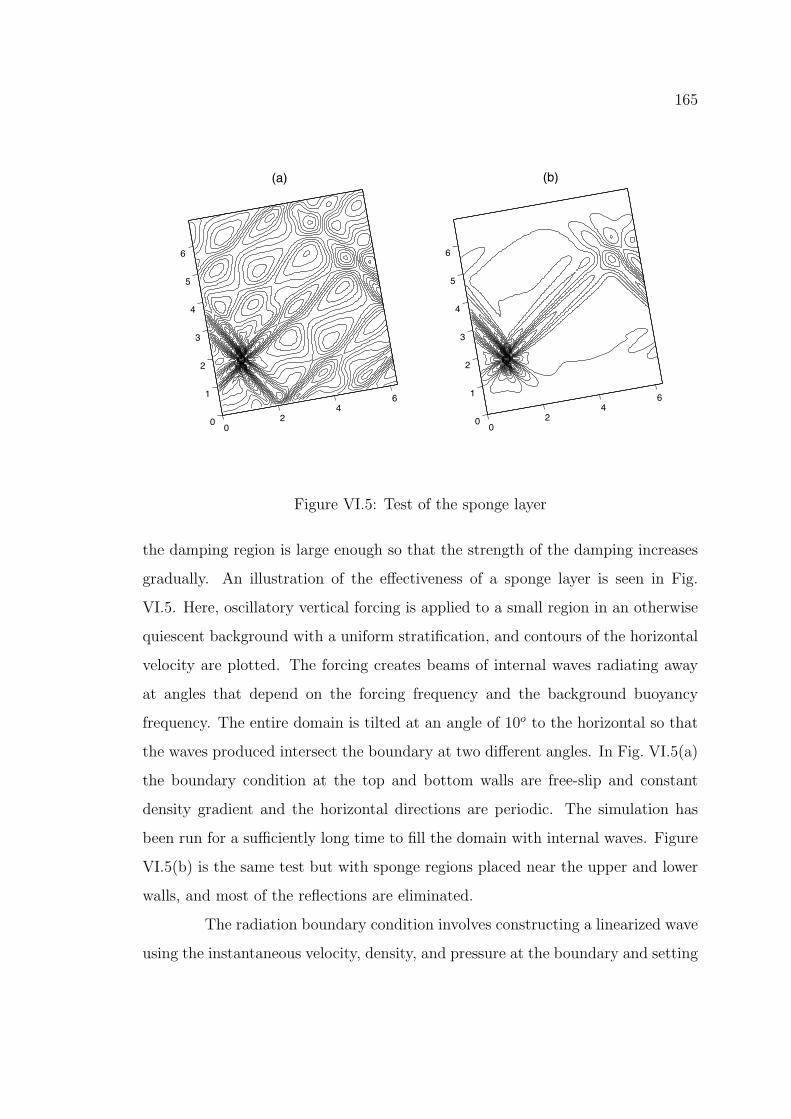
Figure VI.5: Test of the sponge layer

the damping region is large enough so that the strength of the damping increases

gradually. An illustration of the e↵ectiveness of a sponge layer is seen in Fig.

VI.5. Here, oscillatory vertical forcing is applied to a small region in an otherwise

quiescent background with a uniform stratification, and contours of the horizontal

velocity are plotted. The forcing creates beams of internal waves radiating away

at angles that depend on the forcing frequency and the background buoyancy

frequency. The entire domain is tilted at an angle of 10o to the horizontal so that

the waves produced intersect the boundary at two di↵erent angles. In Fig. VI.5(a)

the boundary condition at the top and bottom walls are free-slip and constant

density gradient and the horizontal directions are periodic. The simulation has

been run for a su�ciently long time to fill the domain with internal waves. Figure

VI.5(b) is the same test but with sponge regions placed near the upper and lower

walls, and most of the reflections are eliminated.

The radiation boundary condition involves constructing a linearized wave

using the instantaneous velocity, density, and pressure at the boundary and setting

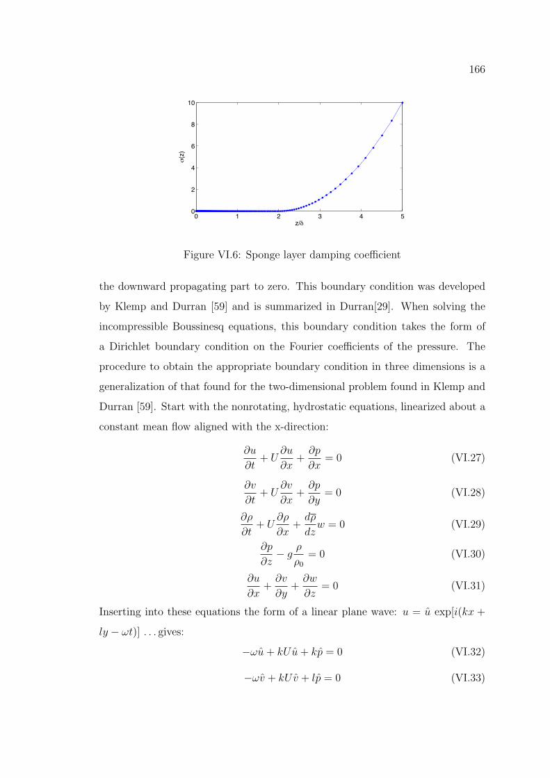
166

0 1 2 3 4 50

2

4

6

8

10

z/d

s(z)

Figure VI.6: Sponge layer damping coe�cient

the downward propagating part to zero. This boundary condition was developed

by Klemp and Durran [59] and is summarized in Durran[29]. When solving the

incompressible Boussinesq equations, this boundary condition takes the form of

a Dirichlet boundary condition on the Fourier coe�cients of the pressure. The

procedure to obtain the appropriate boundary condition in three dimensions is a

generalization of that found for the two-dimensional problem found in Klemp and

Durran [59]. Start with the nonrotating, hydrostatic equations, linearized about a

constant mean flow aligned with the x-direction:

@u

@t+ U

@u

@x+

@p

@x= 0 (VI.27)

@v

@t+ U

@v

@x+

@p

@y= 0 (VI.28)

@⇢

@t+ U

@⇢

@x+

d⇢

dzw = 0 (VI.29)

@p

@z� g

⇢

⇢0= 0 (VI.30)

@u

@x+

@v

@y+

@w

@z= 0 (VI.31)

Inserting into these equations the form of a linear plane wave: u = u exp[i(kx +

ly � !t)] . . . gives:

�!u + kUu + kp = 0 (VI.32)

�!v + kUv + lp = 0 (VI.33)

167

�!⇢ + kU ⇢� iwd⇢

dz= 0 (VI.34)

@p

@z� g

⇢

⇢0= 0 (VI.35)

iku + ilv +@w

@z= 0 (VI.36)

Eliminating all variables from the above set of equations except for w yields:

N2 k2 + l2

(Uk � !)2w +

@2w

@z2= 0 (VI.37)

Solutions to this equation are of the form:

w = Aexp(iN(k2 + l2)1/2z

Uk � !) + Bexp(�iN(k2 + l2)1/2z

Uk � !). (VI.38)

Since the second term corresponds to waves with upward propagating energy, set

B = 0. Then it follows that

@w

@z= iN

(k2 + l2)1/2

Uk � !w. (VI.39)

An equation relating the pressure to the vertical velocity can be found using the

horizontal momentum and continuity equations:

@w

@z= i�

k2 + l2

Uk � !. (VI.40)

Finally, combining the final two equations gives a relation between the pressure

and vertical velocity:

� =N

(k2 + l2)1/2w. (VI.41)

This equation is very easy to implement in the code used here since the Fourier

modes of the vertical velocity are already known. The equations used above to

obtain the boundary conditions were simplified from the rotating, nonhydrostatic

equations simulated in our DNS and LES studies. Klemp and Durran[59] give the

result of the derivations starting with the linearized rotating non-hydrostatic equa-

tions, but the resulting corrections involve the frequency of the wave, !. Since the

frequency of the waves is not known from the instantaneous fields, applying these

corrections requires storing the boundary data in time [9]. Klemp and Durran[59]

168

report adequate results using the boundary condition given in Eq. VI.41 even when

the flow is rotating and nonhydrostatic as long as the scales considered are not too

large (less than the Rossby radius). Since our domain is small compared to the

Rossby radius and since we also consider a sponge region, the simplified radiation

condition in Eq. VI.41 should su�ce.

VI.4 Wall Model

Near walls the turbulent motions scale with the viscous scale, �⌫ = ⌫/u⌧ .

In order to resolve the energy containing scales near the wall, the LES filter length-

scale and hence the gridspacing need to scale with �⌫ . In the outer region the energy

containing scales are much larger, on the order of order �, which is defined by the ge-

ometry of the problem. The ratio of these lengthscales is �⌫/� = ⌫/(u⌧�) = 1/Re⌧ .

Most CFD codes, including Diablo, are forced to have a grid spacing in the x and

y directions (in the plane of the wall) that do not vary as a function of z (the

wall normal direction). With this requirement and the need to resolve the near

wall viscous scale, the x and y grid spacing must be proportional to �⌫ even in

the outer region. When large Reynolds numbers need to be considered, such as in

geophysical applications, this limitation is prohibitive.

In order to consider large Reynolds number wall bounded flows, a near-

wall model is introduced. The model is only active near the wall, and provides a

boundary condition for the LES which is free to scale with the outer flow. A variety

of near-wall models exist in the engineering and atmospheric science literature.

Constructing a near-wall model for the benthic boundary layer is significantly

easier than in the atmospheric case since we do not need to model surface heat

flux e↵ects since, as we have seen from the DNS and resolved LES, the near wall

region remains unstratified. Recall also from the DNS of the benthic Ekman layer

that the magnitude of the horizontal velocity follows a logarithmic law. This

inspires the use of a model type first proposed by Schumann[94] and later modified

169

by Grotzbach[47] in which it is assumed that the instantaneous plane-averaged

velocity obeys a prescribed logarithmic law.

1 2

2 3

j-1 j j+1

j-1 j j+1

N-1 N

NN-1

G =1/2

G =

Figure VI.7: Grid layout of Diablo with a near-wall model. The wall-normal

velocity is defined at G nodes (open circles) and all other components are defined

at G1/2 nodes (closed circles).

The near-wall model of Schumann [94] proceeds as follows. For Poiseuille

flow, the steady state wall stress is known a priori by integrating the streamwise

momentum equation over the wall-normal coordinate. At steady state the wall

stress must balance the applied pressure forcing. The wall stress can then be used

to estimate the plane averaged velocity at some location in the region where the

log law is expected, say at z+ = 40.

U(z+ = 40) = u⌧ (1

ln(z+ = 40) + B). (VI.42)

Recall that the friction velocity is related to the wall stress by u⌧ =p

⌧w/⇢. The

first LES gridpoint is then placed at this location, z+ = 40, and the boundary

condition supplied from the near-wall model is the local wall stress estimated by

assuming that the ratio of the local stress and velocity is equal to the ratio of the

corresponding plane averages:

⌧13(z = 0)(x, y) =u(x, y, 1)

U(1)< ⌧w > . (VI.43)

The local spanwise wall stress is assumed to be proportional to the local spanwise

velocity:

⌧23(z = 0)(x, y) =2

Re⌧

v(x, y, 1)

z(1). (VI.44)

When a staggered grid is used in the vertical direction, the most natural grid with

this wall-model is with a vertical velocity point and the horizontal momentum

170

flux defined at the wall. The wall stress is then specified according to Eq. VI.43

and used as a boundary condition for the first gridpoint away from the wall. In

addition, the wall-normal velocity, the subgrid stress, and the buoyancy flux are

set to zero at the wall. Diablo has been modified so that when the wall-model

is selected, the location of the wall shifts to the wall-normal velocity points as

illustrated in Figure VI.7.

We are interested in problems where the wall stress is not known a priori,

such as a boundary layer with an oscillating free stream velocity. An extension

of Schumann’s model without a prescribed wall stress was proposed by Grotzbach

[47]. Here the first gridpoint of the LES model is placed at z(1)/� where the

expected corresponding location in wall units lies within the logarithmic region.

Then the plane average of the streamwise velocity at this location from the LES

is used to estimate the friction velocity by iteratively solving

U(1)

u⌧=

1

ln(

z(1)

�

u⌧�

⌫) + B. (VI.45)

The local wall stress is then estimated using the friction velocity and the LES

velocity:

⌧13(z = 0) =u(x, y, 1)

U(1)u2

⌧⇢, (VI.46)

⌧23(z = 0) =v(x, y, 1)

U(1)u2

⌧⇢. (VI.47)

The latter relation was suggested by Piomelli et al. [87]. In steady channel flow, the

plane averaged wall stress estimated by this method will necessarily be the same as

that prescribed by the Schumann model since the same momentum balance must

be satisfied.

The Schumann-Grotzbach near-wall model described above has been im-

plemented in Diablo and tested for unstratified closed channel flow. Closed channel

flow was chosen for validation since it is a well-studied problem and DNS results

are available for comparison. Note that while it is standard for y to be assigned to

the wall-normal direction in the engineering literature, here we will use z to stay

171

consistent with the geophysical studies in the rest of the thesis. The first horizon-

tal velocity point of the LES is placed at z+ = 20 with a constant wall-normal

grid spacing throughout the domain �z+ = 40. We have considered a friction

Reynolds number of Re⌧ = 2000. After de-aliasing, 48 Fourier modes remain in

the horizontal directions which have lengths of Lx = 2 ⇤ ⇡ ⇤ �, and Ly = ⇡ ⇤ �.

Using the number of de-alised modes, the horizontal grid spacing in wall units is

then �x+ = 262 and �y+ = 131. The total number of points used after dealias-

ing is 48 x 48 x 100 in the x, y, and z directions respectively. By comparision, a

DNS at this Reynolds number by Hoyas and Jimenez[53] used grid of 6144 x 633 x

4608, or nearly 18 billion gridpoints! The total number of gridpoints used for this

near-wall model test is then 6500 times fewer than needed for a DNS done at the

same domain size.

101 102 103 10410

12

14

16

18

20

22

24

26DNS

(1/0.41)log(z+ )+5.2

z+

<u>/u*

DMM, NWM-LES

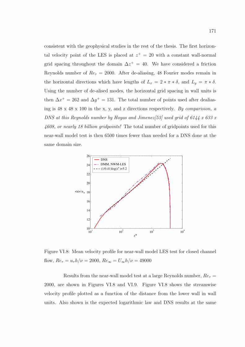
Figure VI.8: Mean velocity profile for near-wall model LES test for closed channel

flow, Re⌧ = u⌧h/⌫ = 2000, Re1 = U1h/⌫ = 49000

Results from the near-wall model test at a large Reynolds number, Re⌧ =

2000, are shown in Figures VI.8 and VI.9. Figure VI.8 shows the streamwise

velocity profile plotted as a function of the distance from the lower wall in wall

units. Also shown is the expected logarithmic law and DNS results at the same

172

Reynolds number by Hoyas and Jimenez [53]. The agreement between the mean

velocity using the near-wall model, the expected log law, and the DNS is excellent.

Notably, the near-wall model LES is able to accurately capture the deviation from

the log law near the centerline compared to the DNS. Figure VI.9 shows profiles of

the rms velocity and the Reynolds stress averaged over horizontal planes and time

at steady state. These turbulent profiles include both the resolved and subgrid-

scale components. The dynamic mixed model (DMM) was chosen since it gave

a better mean velocity profile than the dynamic eddy viscosity model (DEVM).

We found that the DMM predicted a larger total turbulent kinetic energy than

the DEVM, and it appears from Figure VI.9 that the energy is larger than might

be expected from a DNS. In addition, the peaks in the rms velocities are too far

from the wall; the peak urms velocity for example is at the second gridpoint at

z+ = 60 whereas DNS studies indicate that it should be near z+ = 15. Since

the peak in turbulent production occurs in the bu↵er layer [89], these di↵erences

in the near-wall turbulence intensities are not unexpected for a near-wall model

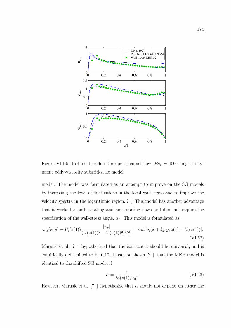
simulation with such a coarse grid. The rms velocity profiles using the near-wall

model at a lower Reynolds number of Re⌧ = 400 in open channel flow are compared

directly to DNS and resolved LES with a dynamic eddy viscosity subgrid model

in Figure VI.10. Here, the peak in the turbulent profiles is underpredicted and

slightly too far away from the wall, but the general agreement is quite good. This

test at Re⌧ = 400 used 32 uniformly spaced points in the vertical direction for the

wall-model simulation compared to 128 and 192 for the resolved LES and DNS,

respectively.

Since the previous relations assumed that the wall stress is aligned with

the outer flow, they cannot be directly applied to the Ekman layer. Instead we

modify the model of Grotzbach [47] as follows. First, the friction velocity and

the magnitude of the wall stress are found by applying the logarithmic law to the

magnitude of the horizontal velocity at the first LES gridpoint as in Eq. VI.45.

Then the plane average wall stresses in the streamwise (x) and cross-stream (y)

173

-1 -0.8 -0.6 -0.4 -0.2 00

0.5

1

1.5

2

2.5

3

3.5

z/h

Ret=2000

<u’u’>1/2/ut NWM� LES

<v’v’>1/2/ut NWM� LES

<w’w’>1/2/ut NWM� LES

<u’u’>1/2/ut DNS

<v’v’>1/2/ut DNS

<w’w’>1/2/ut DNS

Figure VI.9: Turbulent profiles for near-wall model LES test for closed channel

flow using the dynamic mixed subgrid-scale model, Re⌧ = 2000, Re1 = 49000

directions are found by specifying the angle ↵0 between the free stream and the

wall stress:

< ⌧13 >= |⌧w|cos(↵0), < ⌧23 >= |⌧w|sin(↵0). (VI.48)

Then, the x-z component of the local stress is found from:

⌧13(x, y) = u(x, y, 1)< ⌧13 >

U(1), (VI.49)

and the local y-z stress is estimated by taking taking the local maximum of the

following expressions:

⌧23(x, y) = v(x, y, 1)< ⌧23 >

V (1), (VI.50)

⌧23(x, y) = v(x, y, 1)< ⌧13 >

U(1). (VI.51)

The maximum of these two expression is chosen to prevent the spanwise stress

from becoming too small when the mean spanwise stress is small. Equations VI.49

- VI.51 are then used as the boundary condition on the LES velocity field.

An alternative near-wall model formulation for geophysical boundary lay-

ers was proposed by Marusic et al. [? ] which will be referred to as the MKP

174

0 0.2 0.4 0.6 0.8 10

2

4

u rms

0 0.2 0.4 0.6 0.8 10

0.5

1

1.5v rm

s

0 0.2 0.4 0.6 0.8 10

0.5

1

wrm

s

z/h

DNS, 192Resolved LES, 64x128x64Wall model LES, 32

3

3

Figure VI.10: Turbulent profiles for open channel flow, Re⌧ = 400 using the dy-

namic eddy-viscosity subgrid-scale model

model. The model was formulated as an attempt to improve on the SG models

by increasing the level of fluctuations in the local wall stress and to improve the

velocity spectra in the logarithmic region.[? ] This model has another advantage

that it works for both rotating and non-rotating flows and does not require the

specification of the wall-stress angle, ↵0. This model is formulated as:

⌧i,3(x, y) = Ui(z(1))|⌧w|

(U(z(1))2 + V (z(1))2)1/2)� ↵u⇤[ui(x + �d, y, z(1)� Ui(z(1))].

(VI.52)

Marusic et al. [? ] hypothesized that the constant ↵ should be universal, and is

empirically determined to be 0.10. It can be shown [? ] that the MKP model is

identical to the shifted SG model if

↵ =

ln(z(1)/z0). (VI.53)

However, Marusic et al. [? ] hypothesize that ↵ should not depend on either the

175

roughness or the grid-spacing. Indeed, a better agreement with similarity theory

and experimental observations has been obtained with the MKP model compared

to the MKP model for rough wall boundary layers [? ]. The MKP model has been

used in the NWM-LES presented in Chapters III and IV.

VI.5 Computational Algorithm - Channel Flow

Here, we will present the algorithm that Diablo uses for channel flow with

periodic boundary conditions on the velocity in the x1 (x) and x3 (z) directions

and walls bounding the flow in the x2 (y) direction. Wall normal derivatives will

be treated with second order, central finite di↵erences, while the x1 (x) and x3

(z) directions will be treated with a pseudo-spectral method. Time-stepping is

accomplished with a mixed implicit/explicit with all terms involving wall normal

derivatives stepped with Crank-Nicolson and all other terms treated with a low

storage 3rd order Runge-Kutta method. The right hand side of the momentum

equations @ui/@t = ... will be stored in Ri while the Runge-Kutta terms will be

stored in Fi and saved for the next R-K substep. bui, bRi, etc. denote the Fourier

space representations. Care has been taken to order the algorithm so that the

physical and Fourier space arrays can occupy the same location in memory. In

order to clarify the operations, the intermediate and final velocity will be denoted

It is implied that each step is done over all gridpoints in physical space or modes

in Fourier space. For notational simplicity, only those steps which depend on

neighboring points are explicitly indexed.

Below is an algorithm based on the above choices that has been carefully

ordered in order to minimize the number of storage variables and FFT calls.

For t = 1 . . . (# of time steps)

For RK = 1 . . . 3

1. Start building the right hand side array with the previous velocity in Fourier

176

space (bui)

bRi = bui,

2. If (RK > 1) then add the term from the previous RK step

bRi = bRi + ⇣RK�RKbFi

3. Add the pressure gradient to the RHS

bR1 = bR1 � hRK ikxbP

bR2(kx, kz, j) = bR2(kx, kz, j)� hRKbP (k

x

,kz

,j)� bP (kx

,kz

,j�1)�Y (j)

bR3 = bR3 � hRK ikzbP

4. Add Px, the background pressure gradient that drives the flow

bR1(kx = 0, kz = 0, j) = bR1(kx = 0, kz = 0, j)� hRKPx

5. Create a storage variable F that will contain all Runge-Kutta terms and

start with the viscous terms involving horizontal derivatives.

bFi = �⌫(k2x + k2

z)bui,

6. Convert the velocity to physical space

bui ! ui

7. Add the nonlinear terms involving horizontal derivatives to bFbF1 = bF1 � ikx du1u3 � ikx du1u1

bF2 = bF2 � ikx du1u2 � ikz du3u2

bF3 = bF3 � ikz du1u3 � ikz du3u3

(Note that we need 5 independent FFTs here)

8. Now, we are done building the Runge-Kutta terms, add to the right hand

side. We will need to keep bFi for the next RK step, so it should not be

overwritten below this point.

bRi = bRi + �RKhRKbFi

9. Convert the right hand side arrays to physical space

bRi ! Ri,

177

10. Compute the vertical viscous terms and add to the RHS as the explicit part

of Crank-Nicolson.

R1(i, j, k) = R1(i, j, k) +⌫hRK

2�YF (j)

✓u1(i, j + 1, k)� u1(i, j, k)

�Y (j + 1)

◆

� ⌫hRK

2�YF (j)

✓u1(i, j, k)� u1(i, j � 1, k)

�Y (j)

◆

R2(i, j, k) = R2(i, j, k) +⌫hRK

2�Y (j)

✓u2(i, j + 1, k)� u2(i, j, k)

�YF (j)

◆

� ⌫hRK

2�Y (j)

✓u2(i, j, k)� u2(i, j � 1, k)

�YF (j � 1)

◆

R3(i, j, k) = R3(i, j, k) +⌫hRK

2�YF (j)

✓u3(i, j + 1, k)� u3(i, j, k)

�Y (j + 1)

◆

� ⌫hRK

2�YF (j)

✓u3(i, j, k)� u3(i, j � 1, k)

�Y (j)

◆

11. Compute the nonlinear terms involving vertical derivatives and add to the

RHS as the explicit part of Crank-Nicolson.

S1 = u1 ⇤ u2

R1(i, j, k) = R1(i, j, k)� hRK

2 (S1(i, j + 1, k)� S1(i, j, k))/�YF (j)

S1 = u3 ⇤ u2

R3(i, j, k) = R3(i, j, k)� hRK

2 (S1(i, j + 1, k)� S1(i, j, k))/�YF (j)

12. Solve the tridiagonal system for the intermediate wall-normal velocity:

v2(i, j, k)� ⌫hRK

2

✓v2(i, j + 1, k)� v2(i, j, k)

�YF (j)� vv2(i, j, k)� v2(i, j � 1, k)

�YF (j � 1)

◆/�Y (j)

+hRK (v2(i, j, k)u2(i, j, k)� v2(i, j � 1, k)u2(i, j � 1, k)) /�Y (j) = R2(i, j, k)

13. Now that we have the new intermediate wall-normal velocity, v2, solve for

the intermediate v1 and v3 using this new velocity.

v1(i, j, k)� ⌫hRK

2

✓v1(i, j + 1, k)� v1(i, j, k)

�Y (j + 1)� v1(i, j, k)� v1(i, j � 1, k)

�Y (j)

◆/�YF (j)

+hRK (v1(i, j + 1, k)v2(i, j + 1, k)� v1(i, j, k)v2(i, j, k)) /�YF (j) = R1(i, j, k)

178

v3(i, j, k)� ⌫hRK

2

✓v3(i, j + 1, k)� v3(i, j, k)

�Y (j + 1)� v3(i, j, k)� v3(i, j � 1, k)

�Y (j)

◆/�YF (j)

+hRK (v3(i, j + 1, k)v2(i, j + 1, k)� v3(i, j, k)v2(i, j, k)) /�YF (j) = R3(i, j, k)

14. Convert the intermediate velocity to Fourier space

vi ! bvi

15. Solve the tridiagonal system for the pressure correction:

�(k2x + k2

z)b�(kx, kz, j) +⇣

b�(kx

,kz

,j+1)�b�(kx

,kz

,j)�Y (j+1) � b�(k

x

,kz

,j)�b�(kx

,kz

,j�1)�Y (j)

⌘/�YF (j)

= ikxbv1(kx, kz, j) + ikzbv3(kx, kz, j) + (bv2(kx, kz, j + 1)� bv2(kx, kz, j))/�YF (j)

(Note that in order to avoid an extra storage array, we can store � in R1

which is no longer needed for this RK step. Also notice that a factor of hRK

has been absorbed into �)

16. Now, use the pressure update to obtain a divergence-free velocity field.

buRK+11 = bv1 � ikx

b�

buRK+12 (kx, kz, j) = bv2(kx, kz, j)� (b�(kx, kz, j)� b�(kx, kz, j � 1))/�Y (j)

buRK+13 bv3 � ikz

b�

(In order to avoid an extra storage array, only one set of velocity arrays are

defined, and this update is done in place.)

17. Finally, update the pressure field using �

bP = bP + b�/hRK

(We need to divide by hRK since this constant has been absorbed into � in

the steps above.)

In all, we have 14 FFT calls per Runge-Kutta substep, and 11 full-sized storage

arrays.

179

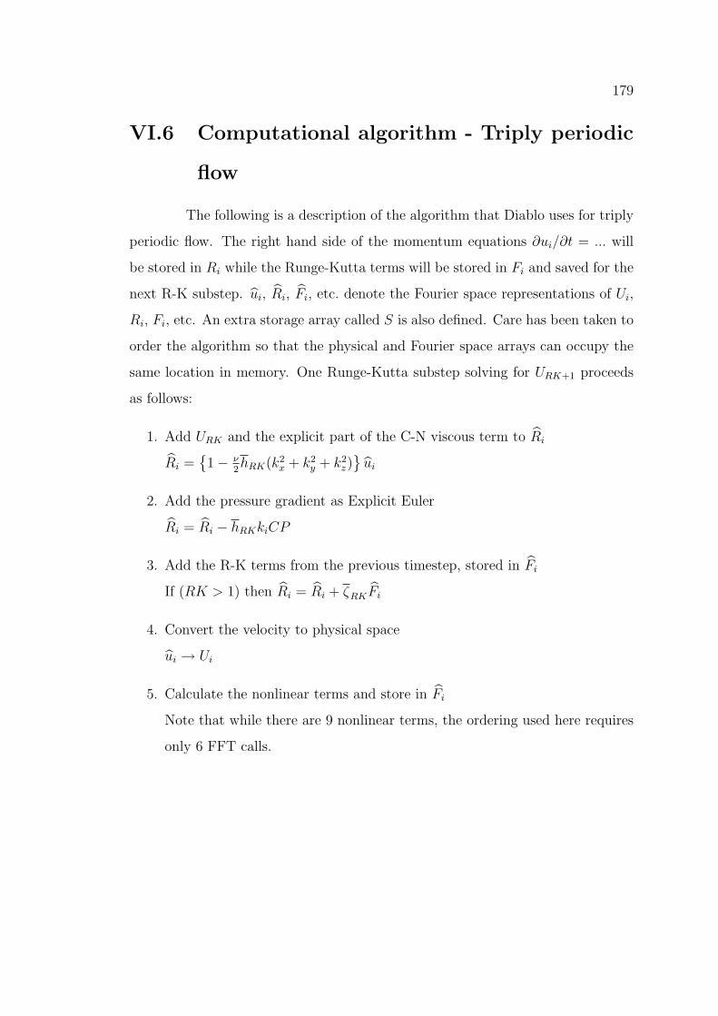
VI.6 Computational algorithm - Triply periodic

flow

The following is a description of the algorithm that Diablo uses for triply

periodic flow. The right hand side of the momentum equations @ui/@t = ... will

be stored in Ri while the Runge-Kutta terms will be stored in Fi and saved for the

next R-K substep. bui, bRi, bFi, etc. denote the Fourier space representations of Ui,

Ri, Fi, etc. An extra storage array called S is also defined. Care has been taken to

order the algorithm so that the physical and Fourier space arrays can occupy the

same location in memory. One Runge-Kutta substep solving for URK+1 proceeds

as follows:

1. Add URK and the explicit part of the C-N viscous term to bRi

bRi =�1� ⌫

2hRK(k2x + k2

y + k2z) bui

2. Add the pressure gradient as Explicit Euler

bRi = bRi � hRKkiCP

3. Add the R-K terms from the previous timestep, stored in bFi

If (RK > 1) then bRi = bRi + ⇣RKbFi

4. Convert the velocity to physical space

bui ! Ui

5. Calculate the nonlinear terms and store in bFi

Note that while there are 9 nonlinear terms, the ordering used here requires

only 6 FFT calls.

180

(a) F1 = U1 ⇤ U1 (j) bF2 = �ikxbF2 � iky

bS

(b) F2 = U1 ⇤ U2 (k) bF3 = �ikxbF3

(c) F3 = U1 ⇤ U3 (l) S = U2 ⇤ U3

(d) S = U2 ⇤ U2 (m) S ! bS

(e) F1 ! bF1 (o) bF2 = bF2 � ikzbS

(f) F2 ! bF2 (p) bF3 = bF3 � ikybS

(g) F3 ! bF3 (q) S = U3 ⇤ U3

(h) S ! bS (r) S ! bS

(i) bF1 = �ikxbF1 � iky

bF2 � ikzbF3 (s) bF3 = bF3 � ikz

bS

6. Add the Runge-Kutta term to the right hand side

bRi = bRi + �RKhRKbFi

7. Solve for the intermediate velocity. Since the system is diagonal, this is easy.

bui = bRi/{1 + ⌫2hRK(k2

x + k2y + k2

z)}

8. Calculate the pressure update � that will make the velocity divergence free

b� = �ikibui/(k2x + k2

y + k2z)

9. Project the velocity to get a divergence free field

bui = bui � ikib�

10. Finally, update the pressure field using �

bp = bp + b�/hRK

In all, we have 9 FFT calls per Runge-Kutta substep, and 11 full-sized storage

arrays.

VI.7 Parallel Computing for CFD

The basic goal of parallel computing for fluid dynamics is to allow us

to solve larger problems on several computers (or several processors within one

computer) more quickly than would be possible on a single computer. For direct

181

numerical simulations (DNS) at large Reynolds numbers, parallel computation

often becomes a necessity owing both to speed and memory limitations. Solving the

Navier-Stokes equations involves performing the same set of operations at a large

number of gridpoints, an indication that parallel computing may be e↵ective for

this problem. There are two basic approaches to parallel programming depending

on the type of hardware that is being used, specifically whether memory is shared

or distributed among the processors. It is now becoming common for new PCs to

use CPUs with multiple cores on a single silicon chip, or to have multiple CPUs

within one computer. These are examples of shared memory systems. It has

become less common for supercomputers to share memory among all processors,

but often processors within a single node are able to share memory. An example of

a distributed memory system would be a cluster of PCs connected via a network,

or separate nodes of a supercomputer. The task of programming to take advantage

of shared and distributed memory systems is quite di↵erent and will be discussed

below.

For shared memory systems, a set of tasks is split into multiple threads

each of which is able to access all of the address space. This e↵ectively eliminates

the need for communication between threads. The main task of the programmer

is then to distribute the computational tasks among the threads with the goal

of achieving an adequate load balance and minimizing the amount of time that

any thread must wait for the others to complete a task. Since the threads utilize

the same address space, it is important to ensure that they do not interfere with

each other. In order to prevent this from occuring, synchronization (or barrier)

commmands are used to make sure that all threads have reached the specified

point before proceeding further. A standard low-level set of thread commands

is known as POSIX. This is commonly used in system-level programming and

gives the programmer full control over the threads, but also requires significant

modifications to a serial code.

The OpenMP standard provides a higher-level set of constructs for pro-

182

! The first block of code will be executed by a single thread only

!$OMP PARALLEL !Any code here will be executed by all threads

!$OMP BARRIER ! This statement tells threads to wait here until all threads have reac

hed this point

!$OMP END PARALLEL!The threads will wait at the end parallel section before proceeding

! Subsequent code will be executed by a single thread until the next OMP directive is reached

! Here is an example of a loop parallelized with OpenMP:! On an OpenMP compatible compiler, the DO I loop will be distributed among the active threads!$OMP DO DO I=1,NX

! Stuff END DO

!$OMP END DO

Figure VI.11: Example of a Fortran code parallelized with OpenMP for shared

memory systems

graming in a shared memory environment. An OpenMP compiler translates a set

of compiler directives (which are ignored as comments to a serial compiler) into

POSIX thread commands. This process is analogous to a high level programming

language such as Fortran translating a program into assembly language. An ex-

ample of how to implement OpenMP compiler directives is shown in Figure VI.11.

See Chandra et al. [20] for an introduction to parallel computing with OpenMP.

On distributed memory systems, memory is local to each process and

other processes are unable to access it directly. An example of this type of system

is a so-called ‘beowulf cluster’ which consists of a number of personal computers

connected through a network. Many modern supercomputers use a combination of

distributed and shared memory with memory distributed over a number of nodes

each consisting of several processors in a shared memory configuration. There

are several models for parallel computing on distributed memory systems. Three

examples are the manager/worker, distributed data, and the pipeline models.

183

A manager/worker model assigns one process to be the manager which

delegates tasks to the worker processes. This model works well on unbalanced

systems where some processes are much faster than others. The fast processes

may finish a job, return the data, and be assigned a new task before the slower

processes finish. In addition, if all data is stored on the manager process, this

model can be used on unreliable networks. If one process goes o✏ine before it

has completed its job, the manager can then redirect the job to another process.

However, for large simulations in CFD, it is often not possible to store the full flow

domain in memory on a single process.

The distributed data model is useful when the same set of operations

are to be performed on a large block of data, as is generally the case in CFD.

With this model it is not necessary to ever store all of the data on one process

and each process is treated equally. Typically a single source code is copied to

all processes and excecuted locally on a set of data. Whenever data is required

from a remote process, the execution of the code must halt until the appropriate

data is recieved. Load balancing is important for this model in order to minimize

the wait time necessary before a synchronized communication. In addition, since

communication tends to be the most time-instensive step in a parallel algorithm,

it is important to minimize the amount of data sent between processes.

The third model, the pipeline approach, is required when one piece of data

must be operated on by all processes. In the limit when each process must wait

until receiving data from its neighbor, this model becomes even worse than a serial

algorithm (the speedup factor becomes less than one) since the communication

takes some amount of time. Because of this, it is important to structure the

algorithm so that as many processes as possible are active at a given time. This

model has been used in the parallel channel flow Diablo for the solve of a tridiagonal

system using the Thomas algorithm. This will be discussed in more detail below.

The most common programming construct for distributed memory sys-

tems is the Message Passing Interface (MPI) which is a standardized library of

184

Table VI.1: Essential MPI routines

MPI INIT Initialize MPIMPI COMM SIZE Get the total number of processesMPI COMM RANK Obtain the rank of the current processMPI SEND Send data to one other processMPI RECV Recieve data from another processMPI FINALIZE Terminate MPI

subroutines that allow the user to direct the communication between processes[46].

While the MPI standard contains many subroutines, only six routines are essen-

tial [44] as listed in Table 1. Unlike OpenMP where compiler directives look like

comments to a serial compiler, compiling an MPI program requires that the MPI

libraries are installed on the local system. In order to allow a single source code

to run on serial and parallel systems, Diablo has been written with all subroutines

that use the MPI libraries in a separate file from the serial code. The Makefile then

determines if MPI will be used, and if not substitutes an empty set of subroutines

in place of the MPI calls.

(a) (b) (c)

Figure VI.12: Domain decomposition options, splitting the domain along (a) one

axis, (b) two axes, and (c) three axes

An important step when writing a distributed memory parallel algorithm

is to decide how to distribute the data among the processes. A schematic of the

three possible choices is shown in Figure VI.12. By decomposing the domain along

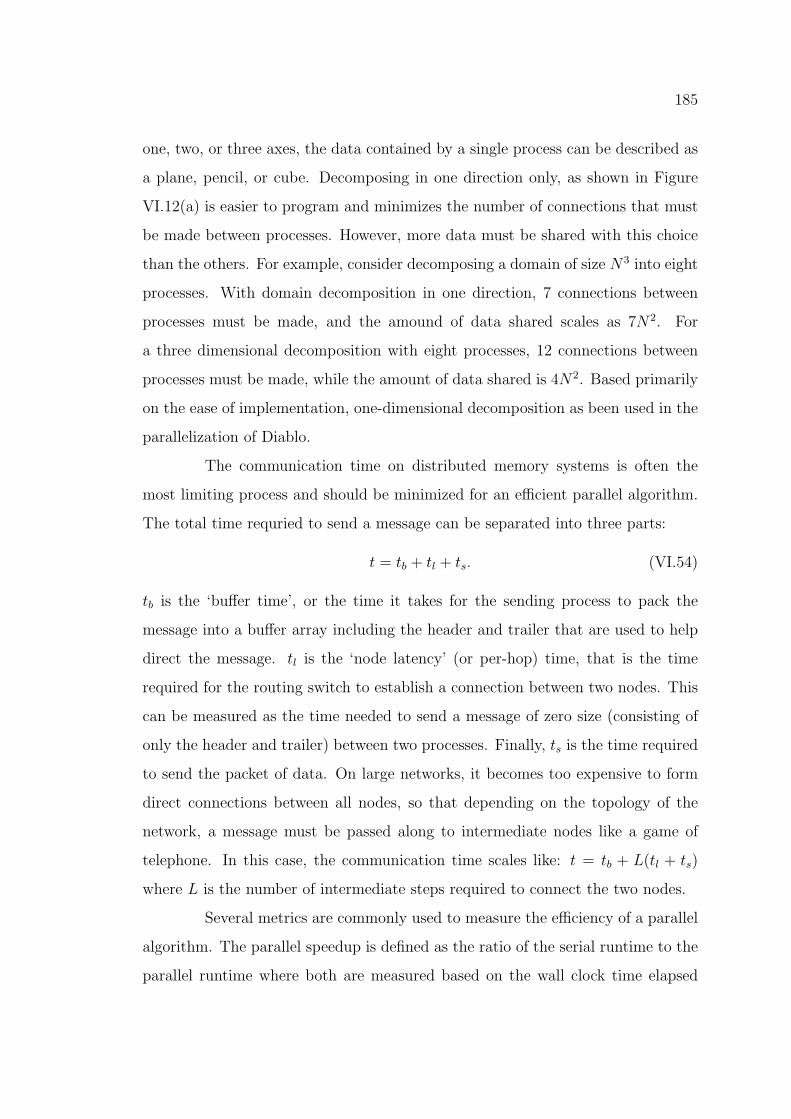
185

one, two, or three axes, the data contained by a single process can be described as

a plane, pencil, or cube. Decomposing in one direction only, as shown in Figure

VI.12(a) is easier to program and minimizes the number of connections that must

be made between processes. However, more data must be shared with this choice

than the others. For example, consider decomposing a domain of size N3 into eight

processes. With domain decomposition in one direction, 7 connections between

processes must be made, and the amound of data shared scales as 7N2. For

a three dimensional decomposition with eight processes, 12 connections between

processes must be made, while the amount of data shared is 4N2. Based primarily

on the ease of implementation, one-dimensional decomposition as been used in the

parallelization of Diablo.

The communication time on distributed memory systems is often the

most limiting process and should be minimized for an e�cient parallel algorithm.

The total time requried to send a message can be separated into three parts:

t = tb + tl + ts. (VI.54)

tb is the ‘bu↵er time’, or the time it takes for the sending process to pack the

message into a bu↵er array including the header and trailer that are used to help

direct the message. tl is the ‘node latency’ (or per-hop) time, that is the time

required for the routing switch to establish a connection between two nodes. This

can be measured as the time needed to send a message of zero size (consisting of

only the header and trailer) between two processes. Finally, ts is the time required

to send the packet of data. On large networks, it becomes too expensive to form

direct connections between all nodes, so that depending on the topology of the

network, a message must be passed along to intermediate nodes like a game of

telephone. In this case, the communication time scales like: t = tb + L(tl + ts)

where L is the number of intermediate steps required to connect the two nodes.

Several metrics are commonly used to measure the e�ciency of a parallel

algorithm. The parallel speedup is defined as the ratio of the serial runtime to the

parallel runtime where both are measured based on the wall clock time elapsed

186

E

# Processors

(a)

E

Problem Size

(b)

1

0

1

0

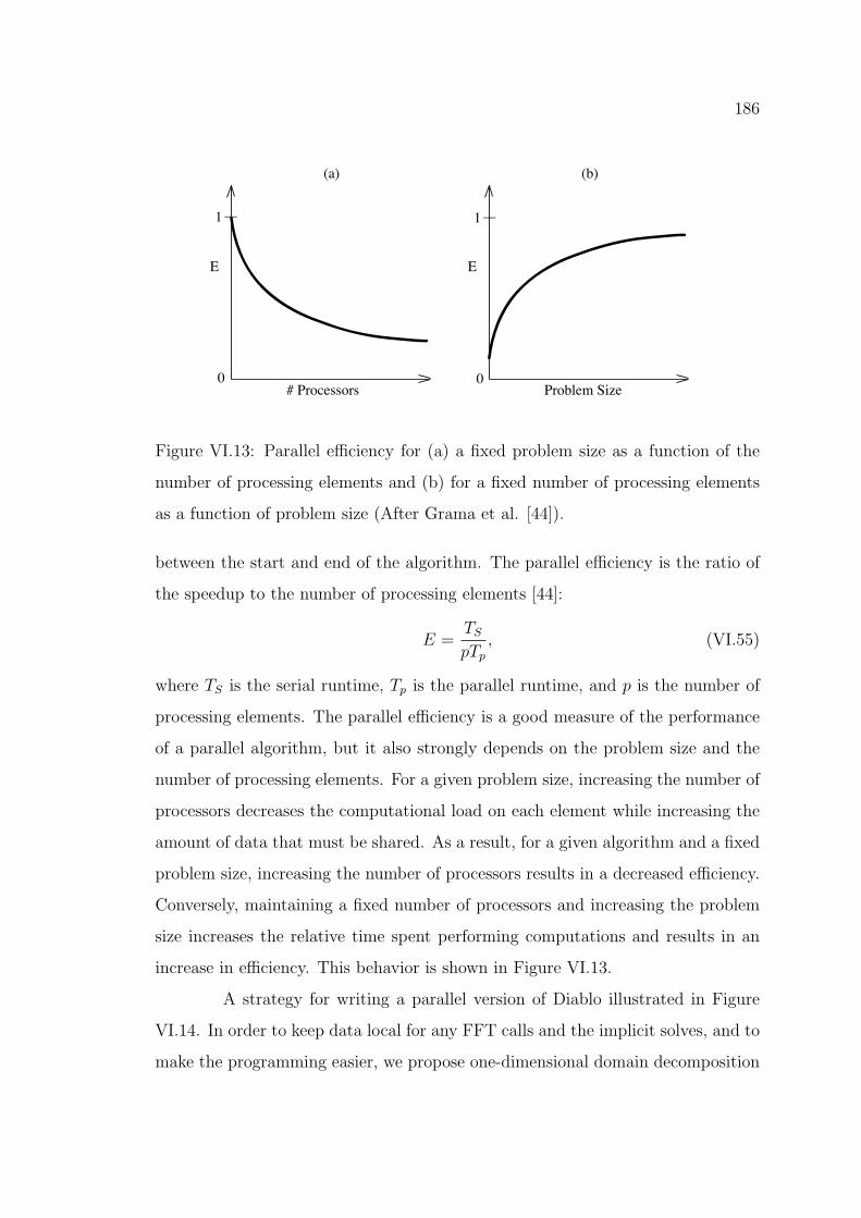
Figure VI.13: Parallel e�ciency for (a) a fixed problem size as a function of the

number of processing elements and (b) for a fixed number of processing elements

as a function of problem size (After Grama et al. [44]).

between the start and end of the algorithm. The parallel e�ciency is the ratio of

the speedup to the number of processing elements [44]:

E =TS

pTp, (VI.55)

where TS is the serial runtime, Tp is the parallel runtime, and p is the number of

processing elements. The parallel e�ciency is a good measure of the performance

of a parallel algorithm, but it also strongly depends on the problem size and the

number of processing elements. For a given problem size, increasing the number of

processors decreases the computational load on each element while increasing the

amount of data that must be shared. As a result, for a given algorithm and a fixed

problem size, increasing the number of processors results in a decreased e�ciency.

Conversely, maintaining a fixed number of processors and increasing the problem

size increases the relative time spent performing computations and results in an

increase in e�ciency. This behavior is shown in Figure VI.13.

A strategy for writing a parallel version of Diablo illustrated in Figure

VI.14. In order to keep data local for any FFT calls and the implicit solves, and to

make the programming easier, we propose one-dimensional domain decomposition

187

3x Periodic

Pass 1: x,z FFTs

x

y

zPass 2: z,y FFTs

Channel Flow

Transpose Pipelined Thomasalgorithm for 3 implicit

solves and pressure correction

Duct Flow

Pass 1: x-dir FFT

2D Serial Multigrid

Transpose

Cavity Flow

Zebra Multigrid withPipelined Thomas solves in

y-direction for 3 implicitsolves and pressure correction

Figure VI.14: Proposed domain decomposition for MPI version of Diablo

in all cases. With this choice, all parallel communication can be broken down

into three subroutines: ghost cell communication, a parallel data transpose, and a

pipelined Thomas algorithm.

In the case of triply periodic flow, FFTs are needed in all three direc-

tions, and the right hand side of the momentum equation is computed in Fourier

space. When computing nonlinear terms, the pseudo-spectral method is used by

transforming the velocity to physical space, computing the nonlinear product, and

transforming the result back to Fourier space. The Fourier transform is a notori-

ously di�cult algorithm to parallelize since it requires a large amount of non-local

communication. In order to avoid a parallel FFT call, each Runge-Kutta substep

can be divided into a two-pass structure. Linear terms are computed during the

first pass with the domain decomposed across wavenumbers in the y-direction. The

velocity is then partially transformed to physical space by taking an inverse FFT

in the x-z plane. Before taking the inverse FFT in the z-direction, the data must

be made local in the z-direction. This can be accomplished by an MPI all-to-all

transpose to distribute the data in y-z planes. At this point, the velocity is in

physical space and nonlinear products can be computed. The process then pro-

ceeds in reverse to transform the velocity to Fourier space involving one more data

188

transpose. Therefore, the triply periodic algorithm without any scalar advection

requires 6 all-to-all transpose operations per Runge-Kutta step (two for each ve-

locity component). It is expected that the transpose operations will be the most

costly step in this algorithm.

x

y

z

j=1

j=NY(on local process)

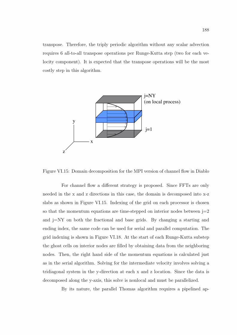
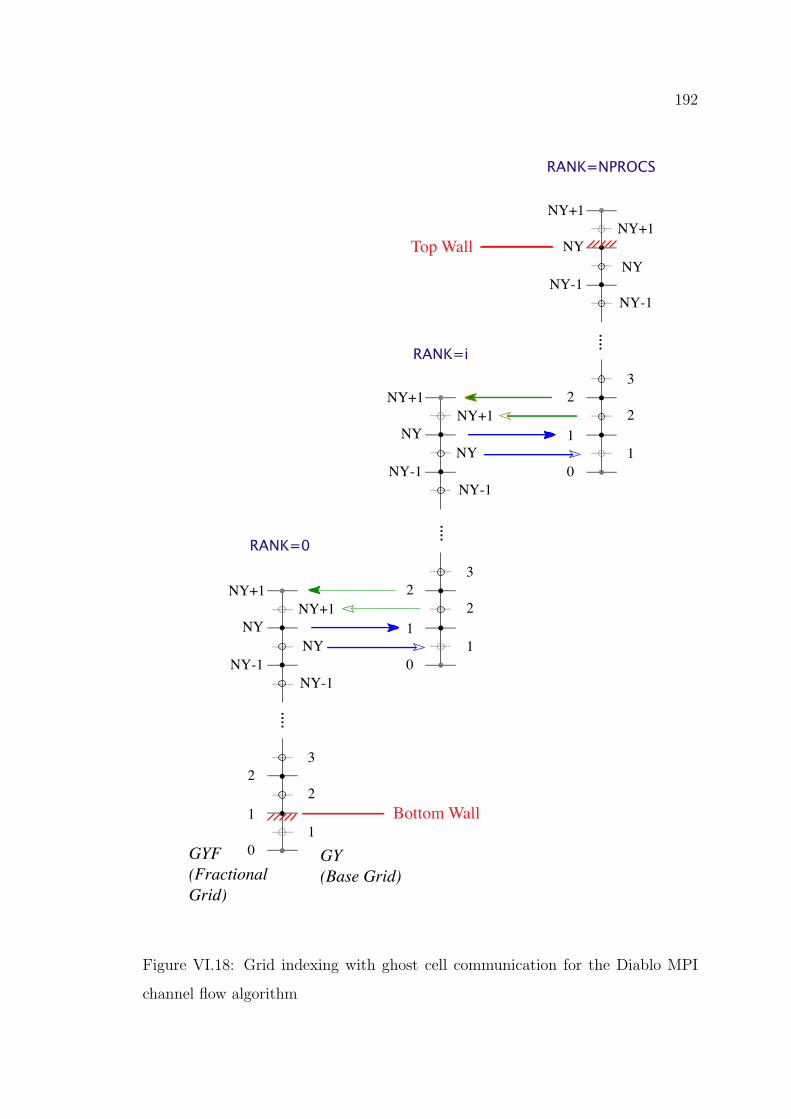
Figure VI.15: Domain decomposition for the MPI version of channel flow in Diablo

For channel flow a di↵erent strategy is proposed. Since FFTs are only

needed in the x and z directions in this case, the domain is decomposed into x-z

slabs as shown in Figure VI.15. Indexing of the grid on each processor is chosen

so that the momentum equations are time-stepped on interior nodes between j=2

and j=NY on both the fractional and base grids. By changing a starting and

ending index, the same code can be used for serial and parallel computation. The

grid indexing is shown in Figure VI.18. At the start of each Runge-Kutta substep

the ghost cells on interior nodes are filled by obtaining data from the neighboring

nodes. Then, the right hand side of the momentum equations is calculated just

as in the serial algorithm. Solving for the intermediate velocity involves solving a

tridiagonal system in the y-direction at each x and z location. Since the data is

decomposed along the y-axis, this solve is nonlocal and must be parallelized.

By its nature, the parallel Thomas algorithm requires a pipelined ap-

189

x

y

z

(a) Rank:

01

nprocs-1

(b) (c) (d)

(e) (f) (g) Idle Process

Active Process

Done withforward-sweep

Done withback-substitution

Forward Sweep

Back-substitution

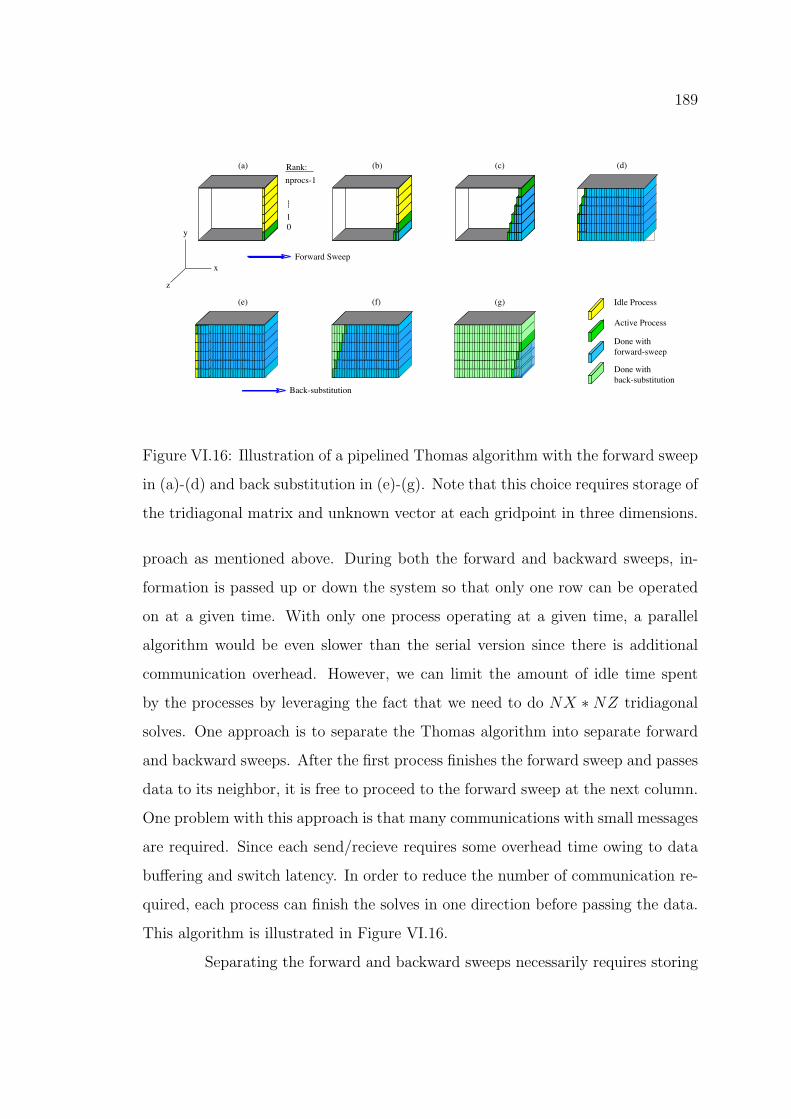
Figure VI.16: Illustration of a pipelined Thomas algorithm with the forward sweep

in (a)-(d) and back substitution in (e)-(g). Note that this choice requires storage of

the tridiagonal matrix and unknown vector at each gridpoint in three dimensions.

proach as mentioned above. During both the forward and backward sweeps, in-

formation is passed up or down the system so that only one row can be operated

on at a given time. With only one process operating at a given time, a parallel

algorithm would be even slower than the serial version since there is additional

communication overhead. However, we can limit the amount of idle time spent

by the processes by leveraging the fact that we need to do NX ⇤ NZ tridiagonal

solves. One approach is to separate the Thomas algorithm into separate forward

and backward sweeps. After the first process finishes the forward sweep and passes

data to its neighbor, it is free to proceed to the forward sweep at the next column.

One problem with this approach is that many communications with small messages

are required. Since each send/recieve requires some overhead time owing to data

bu↵ering and switch latency. In order to reduce the number of communication re-

quired, each process can finish the solves in one direction before passing the data.

This algorithm is illustrated in Figure VI.16.

Separating the forward and backward sweeps necessarily requires storing

190

x

y

z

Rank:

01

nprocs-1Solve 2x2 system

Idle Process Active Process Done withforward-sweep

Done withback-substitution

Forward Sweep Backward Sweep

Figure VI.17: Illustration of a pipelined Thomas algorithm with reduced storage

and a reduced wait-time using bi-directional sovles.

the components of the tridiagonal matrix and the solution vector. The above al-

gorithm therefore requires storage of four three-dimensional arrays. Since memory

requirements can become restrictive for large arrays, this can be a severe limita-

tion. In order to reduce the storage, we can do the forward and backward sweeps

over the x-y axis before moving to the next z-location. This reduces the storage

requirement from 3d arrays to 2d arrays at the expense of added wait time. A code

written in Fortran using MPI for a pipelined Thomas algorithm with stoage in x-y

planes is given in Figure VI.19. A further improvement on this algorithm can be

made by starting forward sweeps at both the uppermost and lowermost process

eliminating the lower and upper diagonal components respectively. Then at the

center of the domain where these solves meet a 2x2 system can be solved quickly on

the center process and back-substitution can again proceed in two directions. This

algorithm is illustrated in Figure VI.17 and reduces the wait time in the previous

algorithm by a factor of two.

The duct and cavity flow version of Diablo can largely leverage the MPI

routines that were described above. For duct flow (with the x-derivatives treated

with the psuedo-spectral method), four Helmholtz equations are solved with a

two-dimensional multigrid routine for the implicit solves for the three velocity

components and the pressure correction. Since the grid and smoothing operations

191

in multigrid are communication intensive, it is desirable to keep this operation

location on each process which implies that data should be decomposed in the y-z

plane. Since it is also important to keep the FFTs in the x-direction local this

suggests that a two-pass algorithm similar to what was proposed above for the 3x

periodic case. For the cavity flow case with finite di↵erences used in all three di-

rections, there is no clear benefit from a two-pass algorithm. Instead, an algorithm

may be used similar to that used in channel flow with ghost cell communication

on each interior node. Then, a parallel version of the three-dimension multigrid

routine will be needed for the velocity and pressure correction solves. One solution

would be to use a zebra variant of multigrid. Smoothing and grid refinement would

then be replaced by a direct tridiagonal solve in one direction for which we already

have a parallel algorithm shown above.

VI.8 Acknowledgments

The material in this chapter was developed after many insightful discus-

sions with Professors Thomas Bewley and Sutanu Sarkar. Robert Martin is also

gratefully acknowledged for developing the first pipelined Thomas algorithm and

the ghost cell communication algorithm.

192

GY(Base Grid)

GYF(FractionalGrid)

0

1

2

1

2

3

NY+1

NY-1

NYNY

NY+1

NY-10

1

2

1

2

3

NY+1

NY-1

NYNY

NY+1

NY-10

1

2

1

2

3

NY+1

NY-1

NYNY

NY+1

NY-1

RANK=0

RANK=i

RANK=NPROCS

Bottom Wall

Top Wall

Figure VI.18: Grid indexing with ghost cell communication for the Diablo MPI

channel flow algorithm

193

C----*|--.---------.---------.---------.---------.---------.---------. SUBROUTINE THOMAS_FORWARD_REAL_MPI(A,B,C,G,NY,NX)C----*|--.---------.---------.---------.---------.---------.---------.

C This subroutine performs the backward sweep of the Thomas algorithmC Input lower, main, and upper diagonals, A, B, C, and rhs GC Returns solution in GC The tridiagonal system is written:C [ b1 c1 0 0 0 ...C [ a2 b2 c2 0 0 ...C [ 0 a3 b3 c3 0 ... INCLUDE 'mpif.h' INCLUDE 'header_mpi'

INTEGER I,J,NY REAL*8 A(0:NX,0:NY), B(0:NX,0:NY), C(0:NX,0:NY), G(0:NX,0:NY)C The following arrays are used to pack data for MPI SEND/RECV REAL*8 OCPACK(3),ICPACK(3)

DO I=0,NXM IF (RANK.NE.0) THENC If we aren't the lowest process, then wait for data CALL MPI_RECV(OCPACK,3,MPI_DOUBLE_PRECISION,RANK-1,1 & ,MPI_COMM_WORLD,status,ierror)C Unpack the data B(I,0)=OCPACK(1) C(I,0)=OCPACK(2) G(I,0)=OCPACK(3) END IF DO J=0,NY-1 A(I,J+1)=-A(I,J+1)/B(I,J) B(I,J+1)=B(I,J+1)+A(I,J+1)*C(I,J) G(I,J+1)=G(I,J+1)+A(I,J+1)*G(I,J) END DO IF (RANK.NE.NPROCS) THEN ICPACK(1)=B(I,NY) ICPACK(2)=C(I,NY) ICPACK(3)=G(I,NY) CALL MPI_SEND(ICPACK,3,MPI_DOUBLE_PRECISION,RANK+1,1 & ,MPI_COMM_WORLD,ierror) END IF END DO

RETURN END

C----*|--.---------.---------.---------.---------.---------.---------. SUBROUTINE THOMAS_BACKWARD_REAL_MPI(A,B,C,G,NY,NX)C----*|--.---------.---------.---------.---------.---------.---------.

C This subroutine performs the backward sweep of the Thomas algorithm

INCLUDE 'mpif.h' INCLUDE 'header_mpi'

INTEGER I,J,NY REAL*8 A(0:NX,0:NY), B(0:NX,0:NY), C(0:NX,0:NY), G(0:NX,0:NY)

DO I=0,NX IF (RANK.NE.NPROCS) THENC If we aren't the highest process, then wait for data CALL MPI_RECV(G(I,NY),1,MPI_DOUBLE_PRECISION,RANK+1 & ,MPI_COMM_WORLD,status,ierror) ELSE C Else, if we are the highest process, then compute the solution at j=NY G(I,NY)=G(I,NY)/B(I,NY) END IF DO J=NY-1,0,-1 G(I,J)=(G(I,J)-C(I,J)*G(I,J+1))/B(I,J) END DO IF (RANK.NE.0) THEN CALL MPI_SEND(G(I,0),1,MPI_DOUBLE_PRECISION,RANK-1,1 & ,MPI_COMM_WORLD,ierror) END IF END DO

RETURN END

Figure VI.19: Source code in Fortran for a pipelined Thomas algorithm with re-

duced storage using MPI.