chapter v results and discussion 5.1...
TRANSCRIPT

Results and Discussion
Some Contribution of Operations Research in Profitable Farm Management 61
CHAPTER – V
RESULTS AND DISCUSSION
5.1 Introduction
The Gujarat state was selected as the project area for the present
research. It is one of the most prosperous states of India owing to its
development in agricultural productivity and industrialization. Agriculture forms
a major part of the state’s economy. It not only provides food grains to the
people but also provides raw materials for agro- based industries.
5.2 Land and Crops
Land
The state occupies approximately 99.00 lakh ha. area under cultivation.
It was revealed from Appendix – I that marginal land holders ( 0.5 to 1.00 ha)
occupied 5.62 lakh ha (5.67 per cent) where as the small holders (1.00 to 2.00
ha), semi medium (2.00 to 4.00 ha), medium (4.00 to 10.00 ha) and large
holders (more than 10 ha) occupied 15.51 lakh ha (15.66 per cent), 27.09
(27.36 per cent), 37.34 lakh ha (37.31 per cent ) and 13.46 lakh ha (13.50 per
cent) respectively. It was found that major share of land holdings was in range
of medium size category. It was found that about 37 percent i.e one third of
state’s farmers were holding land in the range to 4 to 10 ha. Suppose a farmer
had 10 ha land and it could be possible to select any crop from the Table 3.1
with assumptions that all the factors affects the agriculture like soil, climate,
rainfall, irrigation facility are most favorable to the crops selected. Then, by
selecting the maximum profit earning seasonal (four month) crop in each
season for 10 ha land i.e. Groundnut (kharif), Cumin (Rabi) and Paddy (Zaid),
he would be able to earn profit of Rs. 186580 from Groundnut, Rs. 379850
from Cumin and Rs. 396250 from Paddy i.e. total profit of Rs. 962680 per
year from that 10 ha land. The amount seems to be quite good to fulfill his
financial needs.

Results and Discussion
Some Contribution of Operations Research in Profitable Farm Management 62
Crops
The state was engaged in cultivating the crops shown in Table 3.1. It
was found that the state had higher productivity than the national productivity
in the crops like Jowar (10.1 qt/ha), Gram (8.8 qt/ha), Groundnut (22.4
thousand nut/ha) and Castor (18.6 qt/ha). The major horticultural crops grown
in the state were mango, banana, sapota, lime, guava, tomato, potato, onion,
cumin, garlic and fennel. It had highest productivity in guava, potato, onion,
cumin and fennel, while third highest productivity in banana and isabgul in the
country.
5.3 Crops under Study
The crops under study were selected as twelve, twenty and three crops
under kharif, rabi and zaid season respectively. The Cotton (MS) and Cotton
(LS) are long duration (7 to 8 month) kharif crops while Pigeon pea (5 to 6
month), Castor (6 to 8 month), Banana (24 month), Sugarcane and Tobacco
(12 months) were also long duration rabi crops. So when these crops were
selected for the particular season, the farmer had to leave enough land for
that crop in the succeeding season’s land area to be allocated to the ICT.
5.4 Cost of Production and Returns from the Crop
The primary data in a form of structured questionnaire was collected by
divided the state into four zones according to the area of State Agricultural
Universities for the year 2007-08. The number of taluka was predetermined
keeping in view, the availability of resources and gross cropped area in the
districts. The data of ten farmers from three villages were selected at random
from each of the selected taluka. The secondary data were collected from
various Govt. departments. During the imputation procedure for input costs,
the value of purchased input was taken into account as reported by the
farmers with due verification. The apportionment of total cost of cultivation
between the main product and the by-product was done in proportion to their
contribution to the total value of output. The cost concepts were applied as
Results and Discussion
Some Contribution of Operations Research in Profitable Farm Management 63
described in Table 3.2. The data collected were statistically analyzed and
thereby prepared Table 3.3 showing the details of costs of each crop selected
under study per hectare in the state.
In general, the farmers were considered only the amount which they
had paid against different activities of crop cultivation as cost of cultivation for
calculation of profit and they did not considered the rental value of their own
land, interest on value of their owned fixed capital assets, their family member
labor and managerial cost in the cost of cultivation. Considering this concept,
Cost A was taken in to account for profit calculation in Table 3.3. But if one
had to consider the agriculture as an industry than other costs like Cost B,
Cost C1 and Cost C2 also must be taken into consideration as needed for the
profit calculation.
It was also revealed from the Table 3.3 that among all the kharif crops;
Jowar, Maize, Green gram and Black gram were rain fed crops and not
required irrigation thereby in their cost of cultivation, the irrigation cost was
taken as zero. The kharif crops like Sesamum (Rs. 15 per ha), Cluster bean
(Rs 14 per ha) and Bajra (Rs. 4 per ha) required very less supplement
irrigation, but other remaining kharif crops had considerable high irrigation
cost. The rabi crops except Wheat (unir) and Jowar, all the other crops and all
the zaid crops were needed large amount of irrigation. Except the Cow pea
crop, all the crops under study were needed to apply chemical fertilizer. The
prevailing market rate of the main product was somewhat high due to addition
of brokerage of marketing yard, profit of wholesalers, farm product processing
charge, transport cost etc. But the farmers could get the FHP; which was less
compared to the market price. It was found that among the kharif crops,
except Sesamum crop all the crops had income from by-product. Among
twenty rabi crops and three summer crops, except Onion, Garlic, Potato,
Cumin, Fennel, Banana, Tobacco and Chikory; all the crops had also income
from by-product.
Results and Discussion
Some Contribution of Operations Research in Profitable Farm Management 64
The economics of all the selected crops were prepared from Table 3.3
and presented in Table 3.4. It was found that from twelve kharif crops, Cotton
(Long staple) gave the maximum profit but as it is twelve month crop; the land
was to be utilized throughout the year for this single crop only and for another
two season i.e. rabi and summer; no other crop could be cultivated. The
groundnut gave the second highest profit, Paddy gave third highest profit and
both the crop was seasonal (four month) crop. Though the paddy required
highest irrigation but due to the availability of canal water at nominal rate in
the paddy cultivation area i.e. South and Central Gujarat during the kharif and
summer season; the irrigation cost was found very less as compared to other
crops which were cultivated with lift water i.e. from bore or well. In the same
way, it was also found that out of twenty rabi crops, Banana proved the
maximum profit earning crop but it is biennial crop, while the Sugarcane
(Ratoon) was the second highest profit and Tobacco (Culcutti) was the third
highest profit giving crop but both the crops were annual crops. In the summer
season, Paddy was the maximum profit earning crops but it could be
cultivated if the adequate irrigation facility was available.
5.5 ICT based Optimization Model
The ICT based optimization model was very useful to solve farmers
query by taking necessary inputs like the name of famer, village name,
available area for each season, minimum three and maximum five crops
selection for kharif and rabi season; minimum zero and maximum three crops
selection for zaid season, if the irrigation was available. After proper data
feeding to the ICT as shown in flow chart as in Fig. 5.1, when the SHOW
button was selected than another window was displayed showing the
allocation of cultivation area to each crop with total cost of cultivation, total
yield, main product price and income, by-product income, total income and
the profit per crop as well as season wise also (Fig.5.2). The ICT was
accommodated with the facility to change/ update the base data by selecting
the DATABASE button as illustrated in flow chart as in Fig. 5.3. This facility
was very useful to modify the database of ICT for applying recent year cost of

Results and Discussion
Some Contribution of Operations Research in Profitable Farm Management 65
cultivation, yield, main product price, by-product income, total income and
thereby profit per ha of any of the crop under study (Fig.5.4).
Fig. 5.1 Flow chart of ICT Application
Fig. 5.2 Result by ICT

Results and Discussion
Some Contribution of Operations Research in Profitable Farm Management 66
Fig. 5.3 Flow Chart of Data Base updating

Results and Discussion
Some Contribution of Operations Research in Profitable Farm Management 67
(a)
(b)
Fig. 5.4 Updating of ICT Database

Results and Discussion
Some Contribution of Operations Research in Profitable Farm Management 68
5.6 Validation of the ICT based Optimization Model
The validation of the ICT based optimization model was done by
solving the same problem manually by various Simplex methods like Big M
(Penalty), Dual and Two Phase simplex method (Sharma, 2006).
Big M (Penalty) Simplex method
It is the method of removing artificial variables from the basis. In this
method, it assign coefficients to artificial variables, undesirable from the
objective function point of view. If objective function Z is to be minimized, then
a very large positive price (called penalty) is assigned to each artificial
variable. Similarly, if Z is to be maximized, then a very large negative price
(also called penalty) is assigned to each of these variables. The penalty will
be designated by –M for a maximization problem and +M for a minimization
problem, where M>0.
Dual Simplex method
In the LP problem, duality implies that each LP problem can be
analyzed in two different ways but having equivalent solutions. Each LP
problem (both maximization and minimization) stated in its original form has
associated with another LP problem (called dual linear programming problem
or in short dual), which is unique, based on the same data. In general, it is
immaterial which of the two problem is called primal or dual, since the dual of
the dual is primal.
Two Phase Simplex method
In the first phase of this method, the sum of the artificial variables is
minimized subject to the given constraints to get a basic feasible solution of
the LP problem. The second phase minimizes the original objectives function
staring with the basic feasible solution obtained at the end of the first phase.
Since the solution of the LP problem is completed in two phase, this is called

Results and Discussion
Some Contribution of Operations Research in Profitable Farm Management 69
the “Two Phase method”. The advantages of this methods are such as no
assumptions on the original systems of constraints are made, i.e. the system
may be redundant, inconsistent or not solvable in non-negative numbers; it is
easy to obtain an initial basic feasible solution of phase I and the basic
feasible solution (if it exists) obtained at the end of the phase I is used to start
phase II.
5.6.1 Five crops per season
Suppose a ABC farmer (Village: XYZ) wanted to select the crops to be
grown under 100 ha area for the Kharif season from the Table 3.4 as
A1(Jowar), A2 (Maize), A3 (Sesamum), A4 (Green gram) and A5 (Black
gram).
5.6.1.1 Results from developed ICT
The five crop selection and available land for the Kharif season was
used as input to the ICT and it showed the result as shown in Fig. 5.5
Fig. 5.5 Result of five crops selection by ICT

Results and Discussion
Some Contribution of Operations Research in Profitable Farm Management 70
5.6.1.2 Results from LP model
Now for the validation of that result obtained from ICT as in Fig. 5.5,
the same crop selection was applied to the LP model as described in eq. 3.1
with the constraints as eq. 3.2 to 3.7 and solved by Big M (Penalty), Dual and
Two Phase Simplex method as followed considering the profit of each crop
selected as below.
The terminology used in LPP solution by the various Simplex method
are presented as shown in following format.
BV = Basic Variables
MR = Minimum Ratio
+ S = Slack / Surplus variables
Cj = Contribution per unit
Cj – Zj = Net contribution per unit
SV = Solution Values
M = Very large value of coefficient of artificial variable
Sr. No. Crops Profit (Rs/ha)
A11 Jowar 10940
A12 Maize 6241
A13 Sesamum 6054
A14 Green gram 6138
A15 Black gram 4222

Results and Discussion
Some Contribution of Operations Research in Profitable Farm Management 71
A = Artificial variables
Zj = Total contribution of outgoing profit
Problem Statement:
Suppose a farmer wants to grow Jowar, Maize, Sesamum, Green gram and
Black gram crops in the Kharif season. Profit in Rs. per ha from each crop are
10940, 6241, 6054, 6138 and 4222 respectively. The farmer has available
land as 100 ha and he wants to allocate at least 10 % of land for each crop.
This statement has been made from Table 3.4.
Mathematical Formulation of LPP:
Max Z = 10940 A11 + 6241 A12 + 6054 A13 + 6138 A14 + 4222 A15
= 10940 X1 + 6241 X2 + 6054 X3 + 6138 X4 + 4222 X5
Subject to the constraints:
X1 + X2 + X3 + X4 + X5 < 100
X1 > 10
X2 > 10
X3 > 10
X4 > 10
X5 > 10
X1, X2, X3, X4, X5 > 0

Results and Discussion
Some Contribution of Operations Research in Profitable Farm Management 72
5.6.1.2.1 Solution by Big M (Penalty) Simplex Method
For converting inequality to equality, we have to add slack variable S1 in first constraint, subtract surplus variable S2 and add
artificial variable A1 in second constraint, subtract surplus variable S3 and add artificial variable A2 in third constraint, subtract
surplus variable S4 and add artificial variable A3 in fourth constraint, subtract surplus variable S5 and add artificial variable A4 in fifth
constraint; and subtract surplus variable S6 and add artificial variable A5 in sixth constraint i.e.
X1 + X2 + X3 + X4 + X5 + S1 = 100
X1 – S2 + A1 = 10
X2 – S3 + A2 = 10
X3 – S4 + A3 = 10
X4 – S5 + A4 = 10
X5 – S6 + A5 = 10
Now,
Number of variables = n = 16 and
Number of constraints = m = 6
Therefore,
n – m = 10
Results and Discussion
Some Contribution of Operations Research in Profitable Farm Management 73
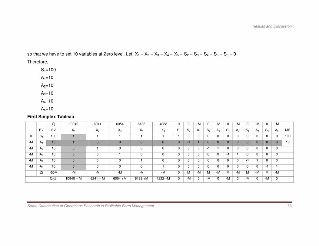
so that we have to set 10 variables at Zero level. Let, X1 = X2 = X3 = X4 = X5 = S2 = S3 = S4 = S5 = S6 = 0
Therefore,
S1=100
A1=10
A2=10
A3=10
A4=10
A5=10
First Simplex Tableau
Cj 10940 6241 6054 6138 4222 0 0 -M 0 -M 0 -M 0 -M 0 -M
BV SV X1 X2 X3 X4 X5 S1 S2 A1 S3 A2 S4 A3 S5 A4 S6 A5 MR
0 S1 100 1 1 1 1 1 1 0 0 0 0 0 0 0 0 0 0 100
-M A1 10 1 0 0 0 0 0 -1 1 0 0 0 0 0 0 0 0 10
-M A2 10 0 1 0 0 0 0 0 0 -1 1 0 0 0 0 0 0
-M A3 10 0 0 1 0 0 0 0 0 0 0 -1 1 0 0 0 0
-M A4 10 0 0 0 1 0 0 0 0 0 0 0 0 -1 1 0 0
-M A5 10 0 0 0 0 1 0 0 0 0 0 0 0 0 0 -1 1
Zj -50M -M -M -M -M -M 0 M -M M -M M -M M -M M -M
Cj-Zj 10940 + M 6241 + M 6054 +M 6138 +M 4222 +M 0 -M 0 -M 0 -M 0 -M 0 -M 0

Results and Discussion
Some Contribution of Operations Research in Profitable Farm Management 74
As the presence of the +ve value in Index Row Cj – Zj, it shows that the solution is not optimum. Now replace A1 by X1, hence the
Second Simplex Tableau
Cj 10940 6241 6054 6138 4222 0 0 -M 0 -M 0 -M 0 -M 0 -M
BV SV X1 X2 X3 X4 X5 S1 S2 A1 S3 A2 S4 A3 S5 A4 S6 A5 R
0 S1 90 0 1 1 1 1 1 1 -1 0 0 0 0 0 0 0 0 90
10940 X1 10 1 0 0 0 0 0 -1 1 0 0 0 0 0 0 0 0
-M A2 10 0 1 0 0 0 0 0 0 -1 1 0 0 0 0 0 0 10
-M A3 10 0 0 1 0 0 0 0 0 0 0 -1 1 0 0 0 0
-M A4 10 0 0 0 1 0 0 0 0 0 0 0 0 -1 1 0 0
-M A5 10 0 0 0 0 1 0 0 0 0 0 0 0 0 0 -1 1
Zj 10940 -40M 10940 -M -M -M -M 0 -10940 10940 M -M M -M M -M M -M
Cj-Zj 0 6241 + M 6054 +M 6138 +M 4222 +M 0 10940 -10940-M -M 0 -M 0 -M 0 -M 0
Here, presence of the +ve value in Index Row Cj – Zj, so again Replace X2 by A2, so that the Third Simplex Tableau as
Cj 10940 6241 6054 6138 4222 0 0 -M 0 -M 0 -M 0 -M 0 -M
BV SV X1 X2 X3 X4 X5 S1 S2 A1 S3 A2 S4 A3 S5 A4 S6 A5 R
0 S1 80 0 0 1 1 1 1 1 -1 0 0 0 0 0 0 1 -1 80
10940 X1 10 1 0 0 0 0 0 -1 1 0 0 0 0 0 0 0 0
6241 X2 10 0 1 0 0 0 0 0 0 -1 1 0 0 0 0 0 0
-M A3 10 0 0 1 0 0 0 0 0 0 0 -1 1 0 0 0 0
-M A4 10 0 0 0 1 0 0 0 0 0 0 0 0 -1 1 0 0 10
-M A5 10 0 0 0 0 1 0 0 0 0 0 0 0 0 0 -1 1
Zj 171810-30M 10940 6241 -M -M -M 0 -10940 10940 -6241 6241 M -M M -M M -M
Cj-Zj 0 0 6054 +M 6138 +M 4222+M 0 10940 -10940-M 6241 -6241+M -M 0 -M 0 -M 0

Results and Discussion
Some Contribution of Operations Research in Profitable Farm Management 75
Again here the presence of the +ve value in Index Row Cj – Zj, so replace A4 by X4, therefore the Fourth Simplex Tableau as
Cj 10940 6241 6054 6138 4222 0 0 -M 0 -M 0 -M 0 -M 0 -M
BV SV X1 X2 X3 X4 X5 S1 S2 A1 S3 A2 S4 A3 S5 A4 S6 A5 R
0 S1 70 0 0 1 0 1 1 1 -1 1 -1 0 0 1 -1 0 0 70
10940 X1 10 1 0 0 0 0 0 -1 1 0 0 0 0 0 0 0 0
6241 X2 10 0 1 0 0 0 0 0 0 -1 1 0 0 0 0 0 0
-M A3 10 0 0 1 0 0 0 0 0 0 0 -1 1 0 0 0 0 10
6138 X4 10 0 0 0 1 0 0 0 0 0 0 0 0 -1 1 0 0
-M A5 10 0 0 0 0 1 0 0 0 0 0 0 0 0 0 -1 1
Zj 233190-20M 10940 6241 -M 6138 -M 0 -10940 10940 -6241 6241 M -M -6138 6138 M -M
Cj-Zj 0 0 6054 +M 0 4222+M 0 10940 -M-10940 6241 -M-6241 -M 0 6138 -6138 -M
-M 0
Here presence of the +ve value in Index Row Cj – Zj, therefore, replace A3 by X3, thereby the Fifth Simplex Tableau as
Cj 10940 6241 6054 6138 4222 0 0 -M 0 -M 0 -M 0 -M 0 -M
BV SV X1 X2 X3 X4 X5 S1 S2 A1 S3 A2 S4 A3 S5 A4 S6 A5 R
0 S1 60 0 0 0 0 1 1 1 -1 1 -1 1 -1 1 -1 0 0 60
10940 X1 10 1 0 0 0 0 0 -1 1 0 0 0 0 0 0 0 0
6241 X2 10 0 1 0 0 0 0 0 0 -1 1 0 0 0 0 0 0
6054 X3 10 0 0 1 0 0 0 0 0 0 0 -1 1 0 0 0 0
6138 X4 10 0 0 0 1 0 0 0 0 0 0 0 0 -1 1 0 0
-M A5 10 0 0 0 0 1 0 0 0 0 0 0 0 0 0 -1 1 10
Zj 293730-10M 10940 6241 6054 6138 -M 0 -10940 10940 -6241 6241 M 6054 -6138 6138 M -M
Cj-Zj 0 0 0 0 4222+M 0 10940 -10940-M 6241 -6241 -M
-M 6054 -M
6138 -6138 -M
-M 0

Results and Discussion
Some Contribution of Operations Research in Profitable Farm Management 76
Now presence of the +ve value in Index Row Cj – Zj again, so that replace A5 by X5 and thereby the Sixth Simplex Tableau as
Cj 10940 6241 6054 6138 4222 0 0 -M 0 -M 0 -M 0 -M 0 -M
BV SV X1 X2 X3 X4 X5 S1 S2 A1 S3 A2 S4 A3 S5 A4 S6 A5 R
0 S1 50 0 0 0 0 0 1 1 -1 1 -1 1 -1 1 -1 1 -1 50
10940 X1 10 1 0 0 0 0 0 -1 1 0 0 0 0 0 0 0 0
6241 X2 10 0 1 0 0 0 0 0 0 -1 1 0 0 0 0 0 0
6054 X3 10 0 0 1 0 0 0 0 0 0 0 -1 1 0 0 0 0
6138 X4 10 0 0 0 1 0 0 0 0 0 0 0 0 -1 1 0 0
4222 X5 10 0 0 0 0 1 0 0 0 0 0 0 0 0 0 -1 1
Zj 335950 10940 6241 6054 6138 4222 0 -10940 10940 -6241 6241 -6054 6054 -6138 6138 -4222 4222
Cj-Zj 0 0 0 0 0 0 10940 -10940-M 6241 -6241+M 6054 -6054-M 6138 -6138 -M
4222 -4222 -M
As presence of the +ve value in Index Row Cj – Zj, replace S1 by S2, hence the Seventh Simplex Tableau as
Cj 10940 6241 6054 6138 4222 0 0 -M 0 -M 0 -M 0 -M 0 -M
BV SV X1 X2 X3 X4 X5 S1 S2 A1 S3 A2 S4 A3 S5 A4 S6 A5
0 S2 50 0 0 0 0 0 1 1 -1 1 -1 1 -1 1 -1 1 -1
10940 X1 60 1 0 0 0 0 1 0 0 1 -1 1 -1 1 -1 1 -1
6241 X2 10 0 1 0 0 0 0 0 0 -1 1 0 0 0 0 0 0
6054 X3 10 0 0 1 0 0 0 0 0 0 0 -1 1 0 0 0 0
6138 X4 10 0 0 0 1 0 0 0 0 0 0 0 0 -1 1 0 0
4222 X5 10 0 0 0 0 1 0 0 0 0 0 0 0 0 0 -1 1
Zj 882950 10940 6241 6054 6138 4222 10940 0 0 4699 -4699 4886 -4886 4802 -4802 6718 -6718
Cj-Zi 0 0 0 0 0 -10940 0 -M -4699 4699-M -4886 4886-M -4802 4802-M -6718 6718-M

Results and Discussion
Some Contribution of Operations Research in Profitable Farm Management 77
Decision: Finally, there is the presence of –ve value in Index Row Cj – Zj of Seventh Simplex Tableau, which shows that the
solution is optimum. Thus, the optimal solution by Big M (Penalty) Simplex Method is Max Z= 882950 with X1=60,
X2=10, X3=10, X4=10, and X5=10
5.6.1.2.2 Solution by Dual Simplex Method
First of all, convert the problem into Standard Primal as shown below.
Max Z = 10940 X1 + 6241 X2 + 6054 X3 + 6138 X4 + 4222 X5
Subject to the constraints:
X1 + X2 + X3 + X4 + X5 < 100
-X1 < 10
-X2 < 10
-X3 < 10
-X4 < 10
-X5 < 10
X1, X2, X3, X4, X5 > 0
The dual of given Standard Primal,
Min Z = 100Y1 – 10Y2 – 10Y3 – 10Y4 – 10Y5 – 10Y6

Results and Discussion
Some Contribution of Operations Research in Profitable Farm Management 78
Subject to the constraints:
Y1 – Y2 > 10940
Y1 – Y3 > 6241
Y1 – Y4 > 6054
Y1 – Y5 > 6138
Y1 – Y6 > 4222
Y1, Y2, Y3, Y4, Y5, Y6 > 0
For converting inequality to equality, we have to subtract surplus variable S1 and add artificial variable A1 in first constraint,
subtract surplus variable S2 and add artificial variable A2 in second constraint, subtract surplus variable S3 and add artificial variable
A3 in third constraint, subtract surplus variable S4 and add artificial variable A4 in fourth constraint and subtract surplus variable S5
and add artificial variable A5 in fifth constraint,
Therefore,
Min Z = 100Y1 – 10Y2 – 10Y3 – 10Y4 – 10Y5 – 10Y6 – 0S1 + MA1 – 0S2 + MA2 – 0S3 + MA3 – 0S4 + MA4 – 0S5 + MA5
Subject to the constraints:
Y1 – Y2 –S1 + A1 = 10940
Y1 –Y3 – S2 + A2 = 6241
Y1 –Y4 – S3 + A3 = 6054
Y1 –Y5– S4 + A4 = 6138
Y1 –Y6– S5 + A5 = 4222
Y1, Y2, Y3, Y4, Y5, Y6 > 0

Results and Discussion
Some Contribution of Operations Research in Profitable Farm Management 79
Now,
Number of variables = n = 16 and
Number of constraints = m = 5
Therefore, n – m = 11,
so that we have to set 11 variables at Zero level.
Let, Y1 = Y2 = Y3 = Y4 = Y5 = Y6 = S1 = S2 = S3 = S4 = S5 = 0
Therefore, A1=10940, A2=6241, A3=6054, A4=6138, A5=4222
First Simplex Tableau
Cj 100 -10 -10 -10 -10 -10 0 M 0 M 0 M 0 M 0 M
BV SV Y1 Y2 Y3 Y4 Y5 Y6 S1 A1 S2 A2 S3 A3 S4 A4 S5 A5 MR
M A1 10940 1 -1 0 0 0 0 -1 1 0 0 0 0 0 0 0 0 10940
M A2 6241 1 0 -1 0 0 0 0 0 -1 1 0 0 0 0 0 0 6241
M A3 6054 1 0 0 -1 0 0 0 0 0 0 -1 1 0 0 0 0 6054
M A4 6138 1 0 0 0 -1 0 0 0 0 0 0 0 -1 1 0 0 6138
M A5 4222 1 0 0 0 0 -1 0 0 0 0 0 0 0 0 -1 1 4222
Zj 23595M 5M -M -M -M -M -M -M M -M M -M M -M M -M M
Cj-Zj 100 - 5M -10 + M -10 + M -10 + M -10 + M -10 + M M 0 M 0 M 0 M 0 M 0

Results and Discussion
Some Contribution of Operations Research in Profitable Farm Management 80
As the presence of the -ve value in Index Row Cj – Zj, it shows that the solution is not optimum. Now replace A5 by Y1, hence the
Second Simplex Tableau
Cj 100 -10 -10 -10 -10 -10 0 M 0 M 0 M 0 M 0 M
BV SV Y1 Y2 Y3 Y4 Y5 Y6 S1 A1 S2 A2 S3 A3 S4 A4 S5 A5 MR
M A1 6718 0 -1 0 0 0 1 -1 1 0 0 0 0 0 0 1 -1 6718
M A2 2019 0 0 -1 0 0 1 0 0 -1 1 0 0 0 0 1 -1 2019
M A3 1832 0 0 0 -1 0 1 0 0 0 0 -1 1 0 0 1 -1 1832
M A4 1916 0 0 0 0 -1 1 0 0 0 0 0 0 -1 1 1 -1 1916
100 Y1 4222 1 0 0 0 0 -1 0 0 0 0 0 0 0 0 -1 1 -
Zj 12485M +
422200
100 -M -M -M -M -100+4M -M M -M M -M M -M M -100+4M 100-4M
Cj-Zj 0 -10+M -10+M -10+M -10+M 90-4M M 0 M 0 M 0 M 0 100-4M -100+5M
Here, presence of the -ve value in Index Row Cj – Zj, so again Replace A3 by Y6, so that the Third Simplex Tableau as
Cj 100 -10 -10 -10 -10 -10 0 M 0 M 0 M 0 M 0 M
BV SV Y1 Y2 Y3 Y4 Y5 Y6 S1 A1 S2 A2 S3 A3 S4 A4 S5 A5 MR
M A1 4886 0 -1 0 1 0 0 -1 1 0 0 1 -1 0 0 0 0 4886
M A2 187 0 0 -1 1 0 0 0 0 -1 1 1 -1 0 0 0 0 187
-10 Y6 1832 0 0 0 -1 0 1 0 0 0 0 -1 1 0 0 1 -1 -
M A4 84 0 0 0 1 -1 0 0 0 0 0 1 -1 -1 1 0 0 84
100 Y1 6054 1 0 0 -1 0 0 0 0 0 0 -1 1 0 0 0 0 -
Zj 5157M +
587080
100 -M -M -90+3M -M -10 -M M -M M -90+3M 90-3M -M M -10 10
Cj-Zj 0 -10+M -10+M 80-3M -10+M 0 M 0 M 0 90-3M -90+4M M 0 10 -10+M

Results and Discussion
Some Contribution of Operations Research in Profitable Farm Management 81
Again here the presence of the -ve value in Index Row Cj – Zj, so replace A4 by Y4, therefore the Fourth Simplex Tableau as
Cj 100 -10 -10 -10 -10 -10 0 M 0 M 0 M 0 M 0 M
BV SV Y1 Y2 Y3 Y4 Y5 Y6 S1 A1 S2 A2 S3 A3 S4 A4 S5 A5 MR
M A1 4802 0 -1 0 0 1 0 -1 1 0 0 0 0 1 -1 0 0 4802
M A2 103 0 0 -1 0 1 0 0 0 -1 1 0 0 1 -1 0 0 103
-10 Y6 1916 0 0 0 0 -1 1 0 0 0 0 0 0 -1 1 1 -1 -
-10 Y4 84 0 0 0 1 -1 0 0 0 0 0 1 -1 -1 1 0 0 -
100 Y1 6138 1 0 0 0 -1 0 0 0 0 0 0 0 -1 1 0 0 -
Zj 4905M +
593800
100 -M -M -10 80+2M -10 0 M -M M -10 10 80+2M 80-2M -10 10
Cj-Zj 0 -10+M -10+M 0 -90-2M 0 0 0 M 0 10 -10+M -80-2M -80+3M 10 -10+M
Again here the presence of the -ve value in Index Row Cj – Zj, so replace A2 by Y5, therefore the Fifth Simplex Tableau as
Cj 100 -10 -10 -10 -10 -10 0 M 0 M 0 M 0 M 0 M
BV SV Y1 Y2 Y3 Y4 Y5 Y6 S1 A1 S2 A2 S3 A3 S4 A4 S5 A5 MR
M A1 4699 0 -1 1 0 0 0 -1 1 1 -1 0 0 0 0 0 0 4699
-10 Y5 103 0 0 -1 0 1 0 1 0 -1 1 0 0 1 -1 0 0 -
-10 Y6 2019 0 0 -1 0 0 1 1 0 -1 1 0 0 0 0 1 -1 -
-10 Y4 187 0 0 -1 1 0 0 1 0 -1 1 1 -1 0 0 0 0 -
100 Y1 6241 1 0 -1 0 0 0 1 0 -1 1 0 0 0 0 0 0 -
Zj 4699M+
601010
100 -M -70+M -10 -10 -10 70-2M M -70+M 70-M -10 10 -10 10 -10 10
Cj-Zj 0 -10+M 60-M 0 0 0 -70+2M 0 70-M -70+2M 10 -10+M 10 -10+M 10 -10+M

Results and Discussion
Some Contribution of Operations Research in Profitable Farm Management 82
Again here the presence of the -ve value in Index Row Cj – Zj, so replace A1 by Y3, therefore the Sixth Simplex Tableau as
Cj 100 -10 -10 -10 -10 -10 0 M 0 M 0 M 0 M 0 M
BV SV Y1 Y2 Y3 Y4 Y5 Y6 S1 A1 S2 A2 S3 A3 S4 A4 S5 A5 MR
-10 Y3 4699 0 -1 1 0 0 0 -1 1 1 -1 0 0 0 0 0 0 -
-10 Y5 4802 0 -1 0 0 1 0 -1 1 0 0 0 0 1 -1 0 0 -
+10 Y6 6718 0 -1 0 0 0 1 -1 1 0 0 0 0 0 0 1 -1 -
-10 Y4 4886 0 -1 0 1 0 0 -1 1 0 0 1 -1 0 0 0 0 -
100 Y1 10940 1 -1 0 0 0 0 -1 1 0 0 0 0 0 0 0 0 -
Zj 882950 100 -60 -10 -10 -10 -10 -60 60 -10 10 -10 10 -10 10 -10 10
Cj-Zj 0 50 0 0 0 0 60 -60+M 10 -10+M 10 -10+M 10 -10+M 10 -10+M
Decision: Finally, there is the presence of +ve value in Index Row Cj – Zj of Sixth Simplex Tableau, which shows that the solution
is optimum. Thus, the optimal solution by Dual Simplex Method is Max Z= 882950 with X1=60, X2=10, X3=10, X4=10,
and X5=10
5.6.1.2.3 Solution by Two Phase Simplex Method
For converting inequality to equality, we have to add slack variable S1 in first constraint, subtract surplus variable S2 and add
artificial variable A1 in second constraint, subtract surplus variable S3 and add artificial variable A2 in third constraint, subtract
surplus variable S4 and add artificial variable A3 in fourth constraint, subtract surplus variable S5 and add artificial variable A4 in fifth
constraint; and subtract surplus variable S6 and add artificial variable A5 in sixth constraint i.e.

Results and Discussion
Some Contribution of Operations Research in Profitable Farm Management 83
The model converted into equality from inequality which is given by
Max Z = 10940 X1 + 6241 X2 + 6054 X3 + 6138 X4 + 4222 X5+ 0S1 – 0S2 + MA1 – 0S3 + MA2 – 0S4 + MA3 – 0S5 + MA4 – 0S6 + MA5
Subject to the constraints:
X1 + X2 + X3 + X4 + X5 +S1 = 100
X1 – S2 + A1 = 10
X2 – S3+ A2 = 10
X3– S4 + A3 = 10
X4 – S5 + A4 = 10
X5 – S6 + A5 = 10
Now,
Number of variables = n = 16 and
Number of constraints = m = 6
Therefore,
n – m = 10
so that we have to set 10 variables at Zero level. Let, X1 = X2 = X3 = X4 = X5 = S2 = S3 = S4 = S5 = S6 = 0
Therefore,
S1=100, A1=10 , A2=10, A3=10, A4=10, A5=10
Assign 0 coefficient to V Xi and V Si and assign -1 coefficient to V Ai in Two Phase Simplex method.
Results and Discussion
Some Contribution of Operations Research in Profitable Farm Management 84
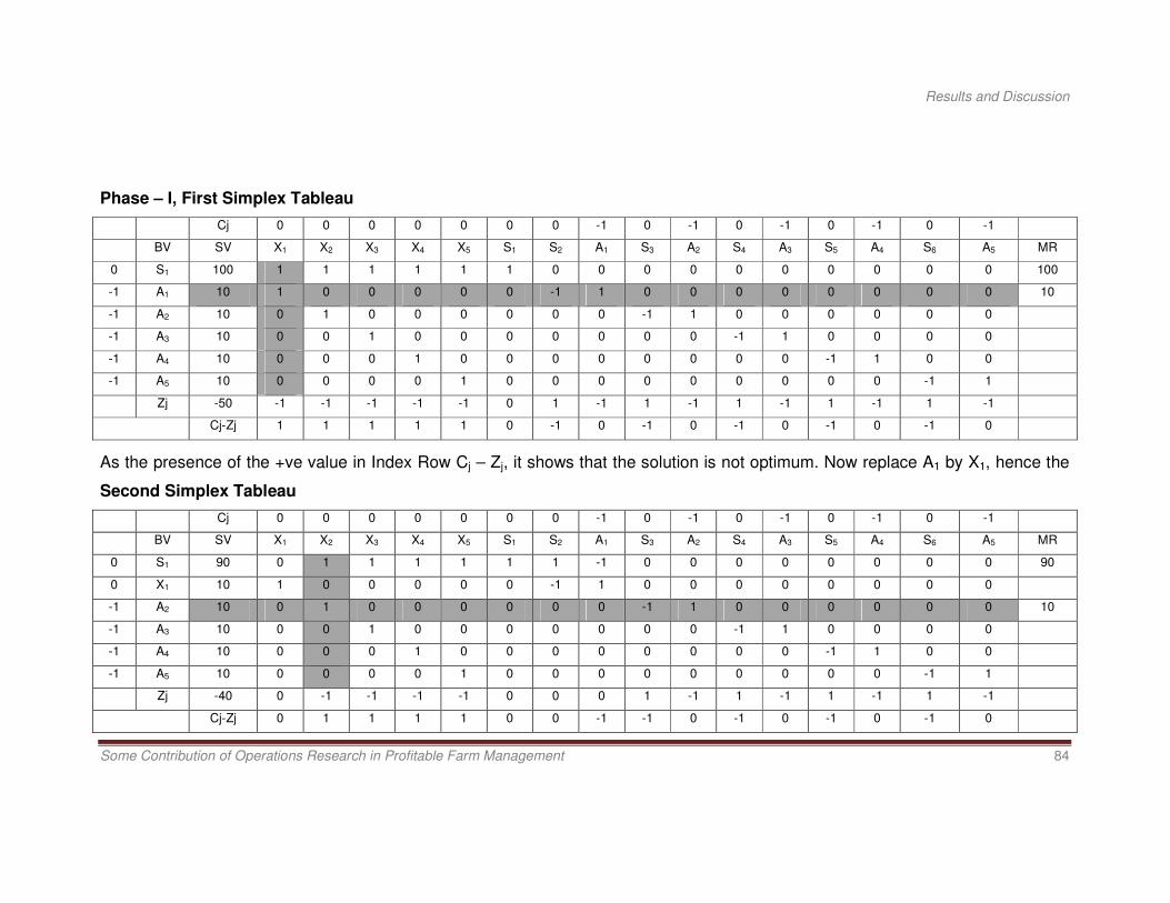
Phase – I, First Simplex Tableau
Cj 0 0 0 0 0 0 0 -1 0 -1 0 -1 0 -1 0 -1
BV SV X1 X2 X3 X4 X5 S1 S2 A1 S3 A2 S4 A3 S5 A4 S6 A5 MR
0 S1 100 1 1 1 1 1 1 0 0 0 0 0 0 0 0 0 0 100
-1 A1 10 1 0 0 0 0 0 -1 1 0 0 0 0 0 0 0 0 10
-1 A2 10 0 1 0 0 0 0 0 0 -1 1 0 0 0 0 0 0
-1 A3 10 0 0 1 0 0 0 0 0 0 0 -1 1 0 0 0 0
-1 A4 10 0 0 0 1 0 0 0 0 0 0 0 0 -1 1 0 0
-1 A5 10 0 0 0 0 1 0 0 0 0 0 0 0 0 0 -1 1
Zj -50 -1 -1 -1 -1 -1 0 1 -1 1 -1 1 -1 1 -1 1 -1
Cj-Zj 1 1 1 1 1 0 -1 0 -1 0 -1 0 -1 0 -1 0
As the presence of the +ve value in Index Row Cj – Zj, it shows that the solution is not optimum. Now replace A1 by X1, hence the
Second Simplex Tableau
Cj 0 0 0 0 0 0 0 -1 0 -1 0 -1 0 -1 0 -1
BV SV X1 X2 X3 X4 X5 S1 S2 A1 S3 A2 S4 A3 S5 A4 S6 A5 MR
0 S1 90 0 1 1 1 1 1 1 -1 0 0 0 0 0 0 0 0 90
0 X1 10 1 0 0 0 0 0 -1 1 0 0 0 0 0 0 0 0
-1 A2 10 0 1 0 0 0 0 0 0 -1 1 0 0 0 0 0 0 10
-1 A3 10 0 0 1 0 0 0 0 0 0 0 -1 1 0 0 0 0
-1 A4 10 0 0 0 1 0 0 0 0 0 0 0 0 -1 1 0 0
-1 A5 10 0 0 0 0 1 0 0 0 0 0 0 0 0 0 -1 1
Zj -40 0 -1 -1 -1 -1 0 0 0 1 -1 1 -1 1 -1 1 -1
Cj-Zj 0 1 1 1 1 0 0 -1 -1 0 -1 0 -1 0 -1 0
Results and Discussion
Some Contribution of Operations Research in Profitable Farm Management 85
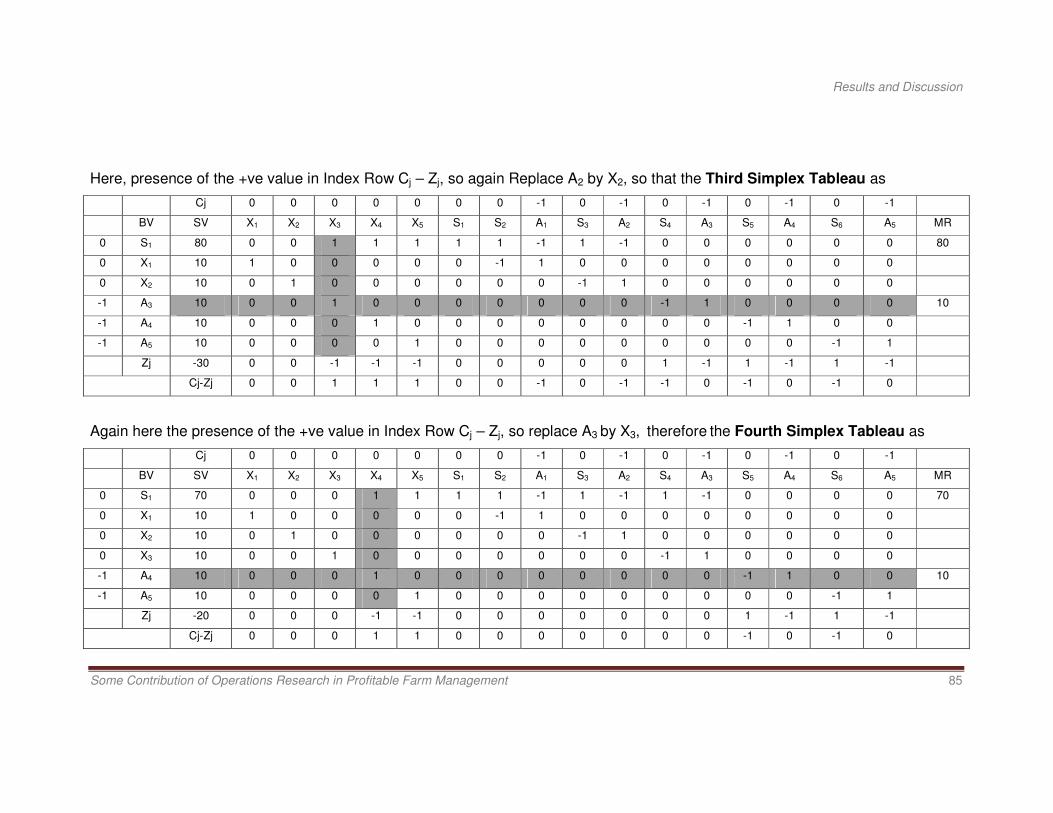
Here, presence of the +ve value in Index Row Cj – Zj, so again Replace A2 by X2, so that the Third Simplex Tableau as
Cj 0 0 0 0 0 0 0 -1 0 -1 0 -1 0 -1 0 -1
BV SV X1 X2 X3 X4 X5 S1 S2 A1 S3 A2 S4 A3 S5 A4 S6 A5 MR
0 S1 80 0 0 1 1 1 1 1 -1 1 -1 0 0 0 0 0 0 80
0 X1 10 1 0 0 0 0 0 -1 1 0 0 0 0 0 0 0 0
0 X2 10 0 1 0 0 0 0 0 0 -1 1 0 0 0 0 0 0
-1 A3 10 0 0 1 0 0 0 0 0 0 0 -1 1 0 0 0 0 10
-1 A4 10 0 0 0 1 0 0 0 0 0 0 0 0 -1 1 0 0
-1 A5 10 0 0 0 0 1 0 0 0 0 0 0 0 0 0 -1 1
Zj -30 0 0 -1 -1 -1 0 0 0 0 0 1 -1 1 -1 1 -1
Cj-Zj 0 0 1 1 1 0 0 -1 0 -1 -1 0 -1 0 -1 0
Again here the presence of the +ve value in Index Row Cj – Zj, so replace A3 by X3, therefore the Fourth Simplex Tableau as
Cj 0 0 0 0 0 0 0 -1 0 -1 0 -1 0 -1 0 -1
BV SV X1 X2 X3 X4 X5 S1 S2 A1 S3 A2 S4 A3 S5 A4 S6 A5 MR
0 S1 70 0 0 0 1 1 1 1 -1 1 -1 1 -1 0 0 0 0 70
0 X1 10 1 0 0 0 0 0 -1 1 0 0 0 0 0 0 0 0
0 X2 10 0 1 0 0 0 0 0 0 -1 1 0 0 0 0 0 0
0 X3 10 0 0 1 0 0 0 0 0 0 0 -1 1 0 0 0 0
-1 A4 10 0 0 0 1 0 0 0 0 0 0 0 0 -1 1 0 0 10
-1 A5 10 0 0 0 0 1 0 0 0 0 0 0 0 0 0 -1 1
Zj -20 0 0 0 -1 -1 0 0 0 0 0 0 0 1 -1 1 -1
Cj-Zj 0 0 0 1 1 0 0 0 0 0 0 0 -1 0 -1 0

Results and Discussion
Some Contribution of Operations Research in Profitable Farm Management 86
Here presence of the +ve value in Index Row Cj – Zj, therefore, replace A4 by X4, thereby the Fifth Simplex Tableau as
Cj 0 0 0 0 0 0 0 -1 0 -1 0 -1 0 -1 0 -1
BV SV X1 X2 X3 X4 X5 S1 S2 A1 S3 A2 S4 A3 S5 A4 S6 A5 MR
0 S1 60 0 0 0 0 1 1 1 -1 1 -1 1 -1 0 0 0 0 60
0 X1 10 1 0 0 0 0 0 -1 1 0 0 0 0 0 0 0 0
0 X2 10 0 1 0 0 0 0 0 0 -1 1 0 0 0 0 0 0
0 X3 10 0 0 1 0 0 0 0 0 0 0 -1 1 0 0 0 0
0 X4 10 0 0 0 1 0 0 0 0 0 0 0 0 -1 1 0 0
-1 A5 10 0 0 0 0 1 0 0 0 0 0 0 0 0 0 -1 1 10
Zj -10 0 0 0 0 -1 0 0 0 0 0 0 0 0 0 1 -1
Cj-Zj 0 0 0 0 1 0 0 -1 0 -1 0 -1 0 -1 0 0
Here presence of the +ve value in Index Row Cj – Zj, therefore, replace A5 by X5, thereby the Sixth Simplex Tableau as
Cj 0 0 0 0 0 0 0 -1 0 -1 0 -1 0 -1 0 -1
BV SV X1 X2 X3 X4 X5 S1 S2 A1 S3 A2 S4 A3 S5 A4 S6 A5 MR
0 S1 50 0 0 0 0 0 1 1 -1 1 -1 1 -1 0 0 1 -1
0 X1 10 1 0 0 0 0 0 -1 1 0 0 0 0 0 0 0 0
0 X2 10 0 1 0 0 0 0 0 0 -1 1 0 0 0 0 0 0
0 X3 10 0 0 1 0 0 0 0 0 0 0 -1 1 0 0 0 0
0 X4 10 0 0 0 1 0 0 0 0 0 0 0 0 -1 1 0 0
0 X5 10 0 0 0 0 1 0 0 0 0 0 0 0 0 0 -1 1
Zj 0 0 0 0 0 0 0 0 0 0 0 0 0 0 0 0 0
Cj-Zj 0 0 0 0 0 0 0 -1 0 -1 0 -1 0 -1 0 -1

Results and Discussion
Some Contribution of Operations Research in Profitable Farm Management 87
Here, all entry of Index Row Cj – Zj is Zero and no artificial variable is present, so the solution is optimum for Phase – I method.
Now converting it into Phase – II method thereby the Phase – II, Seventh Simplex Tableau as
Cj 10940 6241 6054 6138 4222 0 0 0 0 0 0
BV SV X1 X2 X3 X4 X5 S1 S2 S3 S4 S5 S6 MR
0 S1 50 0 0 0 0 0 1 1 1 1 0 1 50
10940 X1 10 1 0 0 0 0 0 -1 0 0 0 0
6241 X2 10 0 1 0 0 0 0 0 -1 0 0 0
6054 X3 10 0 0 1 0 0 0 0 0 -1 0 0
6138 X4 10 0 0 0 1 0 0 0 0 0 -1 0
4222 X5 10 0 0 0 0 1 0 0 0 0 0 -1
Zj 305950 10940 6241 6054 6138 4222 0 -10940 -6241 -6054 -6138 -4222
Cj-Zj 0 0 0 0 0 0 10940 6241 6054 6138 4222
As presence of the +ve value in Index Row Cj – Zj, replace S1 by S2, hence the Eighth Simplex Tableau as
Cj 10940 6241 6054 6138 4222 0 0 0 0 0 0
BV SV X1 X2 X3 X4 X5 S1 S2 S3 S4 S5 S6 MR
0 S2 50 0 0 0 0 0 1 1 1 1 1 1
10940 X1 60 1 0 0 0 0 0 0 1 1 1 1
6241 X2 10 0 1 0 0 0 0 0 -1 0 0 0
6054 X3 10 0 0 1 0 0 0 0 0 -1 0 0
6138 X4 10 0 0 0 1 0 0 0 0 0 -1 0
4222 X5 10 0 0 0 0 1 0 0 0 0 0 -1
Zj 882950 10940 6241 6054 6138 4222 0 0 4699 4886 4802 6718
Cj-Zj 0 0 0 0 0 0 0 -4699 -4886 -4802 -6718

Results and Discussion
Some Contribution of Operations Research in Profitable Farm Management 88
Decision: Finally, there is the presence of –ve value in Index Row Cj – Zj of Eighth Simplex Tableau, which shows that the
solution is optimum. Thus, the optimal solution by Two Phase Simplex Method is Max Z= 882950 with X1=60, X2=10,
X3=10, X4=10, and X5=10
The results by all the three LPP techniques applied manually i.e. Big M (Penalty), Dual and Two Phase methods were
identical and presented in the Table 5.1.
Table 5.1 Result of five crops selection by LPP Technique
Particular Result by Simplex method
Big M Dual Two Phase
Max. Profit = Rs. 882950 Rs. 882950 Rs. 882950
X1, Jowar crop area = 60 ha 60 ha 60 ha
X2, Maize crop area = 10 ha 10 ha 10 ha
X3, Sesamum crop area = 10 ha 10 ha 10 ha
X4, Green gram crop area = 10 ha 10 ha 10 ha
X5, Black gram crop area = 10 ha 10 ha 10 ha

Results and Discussion
Some Contribution of Operations Research in Profitable Farm Management 89
5.6.1.3 Comparison between ICT and LP model results
It was found from Fig. 5.5 and Table 5.1 that by both the tool applied to
the profit maximization problem of farmer ABC for the selection of crops
A1(Jowar), A2 (Maize), A3 (Sesamum), A4 (Green gram) and A5 (Black
gram) in the Kharif season was identical i.e. profit was Rs. 882950 with land
allocation to each crop as 60, 10, 10, 10 and 10 ha respectively which was
also proved that the developed ICT is validated.
5.6.2 Four crops per season
Suppose a ABC farmer (Village: XYZ) wanted to select the crops to be
grown under 100 ha area for the Rabi season from the Table 3.4 as
B1(Wheat Irri.), B2 (Wheat unirri.), B3 (Jowar) and B4 (Pigeon pea) crops.
5.6.2.1 Results from developed ICT
The four crop selection and available land for the Rabi season was
used as input to the ICT and it showed the result as shown in Fig. 5.6
Fig. 5.6 Result of four crops selection by ICT
Results and Discussion
Some Contribution of Operations Research in Profitable Farm Management 90
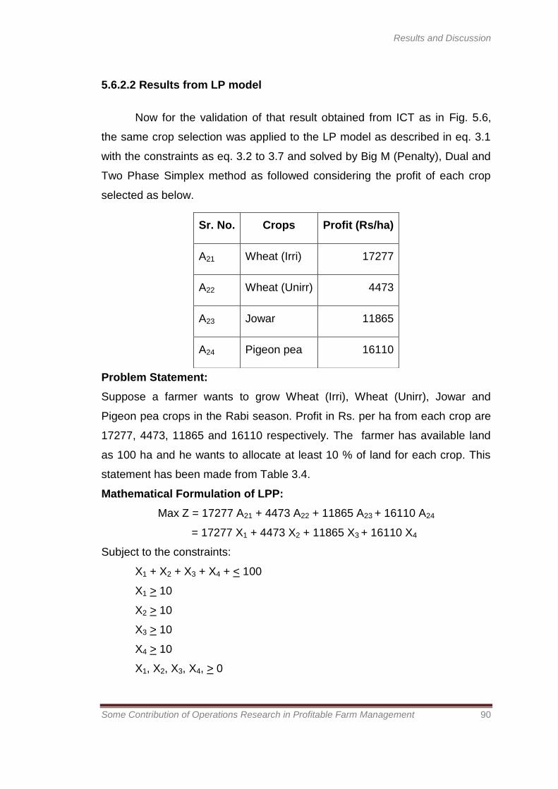
5.6.2.2 Results from LP model
Now for the validation of that result obtained from ICT as in Fig. 5.6,
the same crop selection was applied to the LP model as described in eq. 3.1
with the constraints as eq. 3.2 to 3.7 and solved by Big M (Penalty), Dual and
Two Phase Simplex method as followed considering the profit of each crop
selected as below.
Problem Statement:
Suppose a farmer wants to grow Wheat (Irri), Wheat (Unirr), Jowar and
Pigeon pea crops in the Rabi season. Profit in Rs. per ha from each crop are
17277, 4473, 11865 and 16110 respectively. The farmer has available land
as 100 ha and he wants to allocate at least 10 % of land for each crop. This
statement has been made from Table 3.4.
Mathematical Formulation of LPP:
Max Z = 17277 A21 + 4473 A22 + 11865 A23 + 16110 A24
= 17277 X1 + 4473 X2 + 11865 X3 + 16110 X4
Subject to the constraints:
X1 + X2 + X3 + X4 + < 100
X1 > 10
X2 > 10
X3 > 10
X4 > 10
X1, X2, X3, X4, > 0
Sr. No. Crops Profit (Rs/ha)
A21 Wheat (Irri) 17277
A22 Wheat (Unirr) 4473
A23 Jowar 11865
A24 Pigeon pea 16110

Results and Discussion
Some Contribution of Operations Research in Profitable Farm Management 91
5.6.2.2.1 Solution by Big M (Penalty) Simplex Method
For converting inequality to equality, we have to add slack variable S1 in first constraint, subtract surplus variable S2 and add
artificial variable A1 in second constraint, subtract surplus variable S3 and add artificial variable A2 in third constraint, subtract
surplus variable S4 and add artificial variable A3 in fourth constraint, subtract surplus variable S5 and add artificial variable A4 in fifth
constraint; i.e.
X1 + X2 + X3 + X4 + S1 = 100
X1 – S2 + A1 = 10
X2 – S3 + A2 = 10
X3 – S4 + A3 = 10
X4 – S5 + A4 = 10
Now,
Number of variables = n = 13 and
Number of constraints = m = 5
Therefore,
n – m = 8
so that we have to set 8 variables at Zero level. Let, X1 = X2 = X3 = X4 = S2 = S3 = S4 = S5 = 0
Therefore, S1=100, A1=10, A2=10, A3=10, A4=10
Results and Discussion
Some Contribution of Operations Research in Profitable Farm Management 92
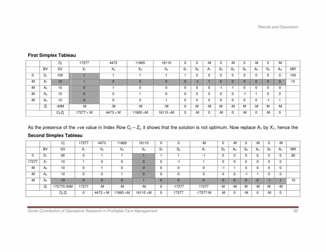
First Simplex Tableau
Cj 17277 4473 11865 16110 0 0 -M 0 -M 0 -M 0 -M
BV SV X1 X2 X3 X4 S1 S2 A1 S3 A2 S4 A3 S5 A4 MR
0 S1 100 1 1 1 1 1 0 0 0 0 0 0 0 0 100
-M A1 10 1 0 0 0 0 -1 1 0 0 0 0 0 0 10
-M A2 10 0 1 0 0 0 0 0 -1 1 0 0 0 0
-M A3 10 0 0 1 0 0 0 0 0 0 -1 1 0 0
-M A4 10 0 0 0 1 0 0 0 0 0 0 0 -1 1
Zj -40M -M -M -M -M 0 M -M M -M M -M M -M
Cj-Zj 17277 + M 4473 + M 11865 +M 16110 +M 0 -M 0 -M 0 -M 0 -M 0
As the presence of the +ve value in Index Row Cj – Zj, it shows that the solution is not optimum. Now replace A1 by X1, hence the
Second Simplex Tableau
Cj 17277 4473 11865 16110 0 0 -M 0 -M 0 -M 0 -M
BV SV X1 X2 X3 X4 S1 S2 A1 S3 A2 S4 A3 S5 A4 MR
0 S1 90 0 1 1 1 1 1 -1 0 0 0 0 0 0 90
17277 X1 10 1 0 0 0 0 -1 1 0 0 0 0 0 0
-M A2 10 0 1 0 0 0 0 0 -1 1 0 0 0 0
-M A3 10 0 0 1 0 0 0 0 0 0 -1 1 0 0
-M A4 10 0 0 0 1 0 0 0 0 0 0 0 -1 1 10
Zj 172770-30M 17277 -M -M -M 0 -17277 17277 M -M M -M M -M
Cj-Zj 0 4473 + M 11865 +M 16110 +M 0 17277 -17277-M -M 0 -M 0 -M 0

Results and Discussion
Some Contribution of Operations Research in Profitable Farm Management 93
Here, presence of the +ve value in Index Row Cj – Zj, so again Replace A4by X4, so that the Third Simplex Tableau as
Cj 17277 4473 11865 16110 0 0 -M 0 -M 0 -M 0 -M
BV SV X1 X2 X3 X4 S1 S2 A1 S3 A2 S4 A3 S5 A4 MR
0 S1 80 0 1 1 0 1 1 -1 0 0 0 0 1 -1 80
17277 X1 10 1 0 0 0 0 -1 1 0 0 0 0 0 0
-M A2 10 0 1 0 0 0 0 0 -1 1 0 0 0 0
-M A3 10 0 0 1 0 0 0 0 0 0 -1 1 0 0 10
16110 X4 10 0 0 0 1 0 0 0 0 0 0 0 -1 1
Zj 333870 17277 -M -M 16110 0 -17277 17277 M -M M -M -16110 16110
Cj-Zj 0 4473 + M 11865 +M 0 0 17277 -17277-M -M 0 -M 0 16110 -16110-M
Again here the presence of the +ve value in Index Row Cj – Zj, so replace A3 by X3, therefore the Fourth Simplex Tableau as
Cj 17277 4473 11865 16110 0 0 -M 0 -M 0 -M 0 -M
BV SV X1 X2 X3 X4 S1 S2 A1 S3 A2 S4 A3 S5 A4 MR
0 S1 70 0 1 0 0 1 1 -1 0 0 0 0 1 -1 70
17277 X1 10 1 0 0 0 0 -1 1 0 0 0 0 0 0
-M A2 10 0 1 0 0 0 0 0 -1 1 0 0 0 0 10
11865 X3 10 0 0 1 0 0 0 0 0 0 -1 1 0 0
16110 X4 10 0 0 0 1 0 0 0 0 0 0 0 -1 1
Zj 452520-10M 17277 -M 11865 16110 0 -17277 17277 M -M -11865 11865 -16110 16110
Cj-Zj 0 4473 + M 0 0 0 17277 -17277-M -M 0 11865 -11865-M 16110 -16110-M

Results and Discussion
Some Contribution of Operations Research in Profitable Farm Management 94
Here presence of the +ve value in Index Row Cj – Zj, therefore, replace A2 by X2, thereby the Fifth Simplex Tableau as
Cj 17277 4473 11865 16110 0 0 -M 0 -M 0 -M 0 -M
BV SV X1 X2 X3 X4 S1 S2 A1 S3 A2 S4 A3 S5 A4 MR
0 S1 60 0 0 0 0 1 1 -1 1 -1 0 0 1 -1 60
17277 X1 10 1 0 0 0 0 -1 1 0 0 0 0 0 0
4473 X2 10 0 1 0 0 0 0 0 -1 1 0 0 0 0
11865 X3 10 0 0 1 0 0 0 0 0 0 -1 1 0 0
16110 X4 10 0 0 0 1 0 0 0 0 0 0 0 -1 1
Zj 497250 17277 4473 11865 16110 0 -17277 17277 -4473 4473 -11865 11865 -16110 16110
Cj-Zj 0 0 0 0 0 17277 -17277-M 4473 -4473-M 11865 -11865-M 16110 -16110-M
Now presence of the +ve value in Index Row Cj – Zj again, so that replace S1by S2 and thereby the Sixth Simplex Tableau as
Cj 17277 4473 11865 16110 0 0 -M 0 -M 0 -M 0 -M
BV SV X1 X2 X3 X4 S1 S2 A1 S3 A2 S4 A3 S5 A4 MR
0 S2 60 0 0 0 0 1 1 -1 1 -1 0 0 1 -1
17277 X1 70 1 0 0 0 0 0 0 1 -1 0 0 1 0
4473 X2 10 0 1 0 0 0 0 0 -1 1 0 0 0 0
11865 X3 10 0 0 1 0 0 0 0 0 0 1 1 0 0
16110 X4 10 0 0 0 1 0 0 0 0 0 0 0 -1 1
Zj 1533870 17277 4473 11865 16110 16110 4473 -4473 0 0 11865 11865 -11637 11637
Cj-Zj 0 0 0 0 -16110 -4473 4473-M 0 -M -11865 -11865-M 11637 -11637-M

Results and Discussion
Some Contribution of Operations Research in Profitable Farm Management 95
Decision: Finally, there is the presence of –ve value in Index Row Cj – Zj of Seventh Simplex Tableau, which shows that the
solution is optimum. Thus, the optimal solution by Big M (Penalty) Simplex Method is Max Z= 1533870 with X1=70,
X2=10, X3=10 and X4=10
5.6.2.2.2 Solution by Dual Simplex Method
First of all, convert the problem into Standard Primal as shown below.
Max Z = 17277 X1 + 4473 X2 + 11865 X3 + 16110 X4
Subject to the constraints:
X1 + X2 + X3+ X4 < 100
-X1 < 10
-X2 < 10
-X3 < 10
-X4 < 10
X1, X2, X3, X4 > 0
The dual of given Standard Primal, Min Z = 100Y1 – 10Y2 – 10Y3 – 10Y4– 10Y5

Results and Discussion
Some Contribution of Operations Research in Profitable Farm Management 96
Subject to the constraints:
Y1 – Y2 > 17277
Y1 – Y3 > 4473
Y1 – Y4 > 11865
Y1 – Y5> 16110
Y1, Y2, Y3, Y4, Y5 > 0
For converting inequality to equality, we have to subtract surplus variable S1 and add artificial variable A1 in first constraint,
subtract surplus variable S2 and add artificial variable A2 in second constraint, subtract surplus variable S3 and add artificial variable
A3 in third constraint and subtract surplus variable S4 and add artificial variable A4 in third constraint.
Therefore,
Min Z = 100Y1 – 10Y2 – 10Y3 – 10Y4 – 10Y5 – 0S1 + MA1 – 0S2 + MA2 – 0S3 + MA3– 0S4 + MA4
Subject to the constraints:
Y1 – Y2 – S1 + A1 = 17277
Y1 – Y3 – S2 + A2 = 4473
Y1– Y4 – S3 + A3 = 11865
Y1– Y5 – S4 + A4 = 16110
Results and Discussion
Some Contribution of Operations Research in Profitable Farm Management 97
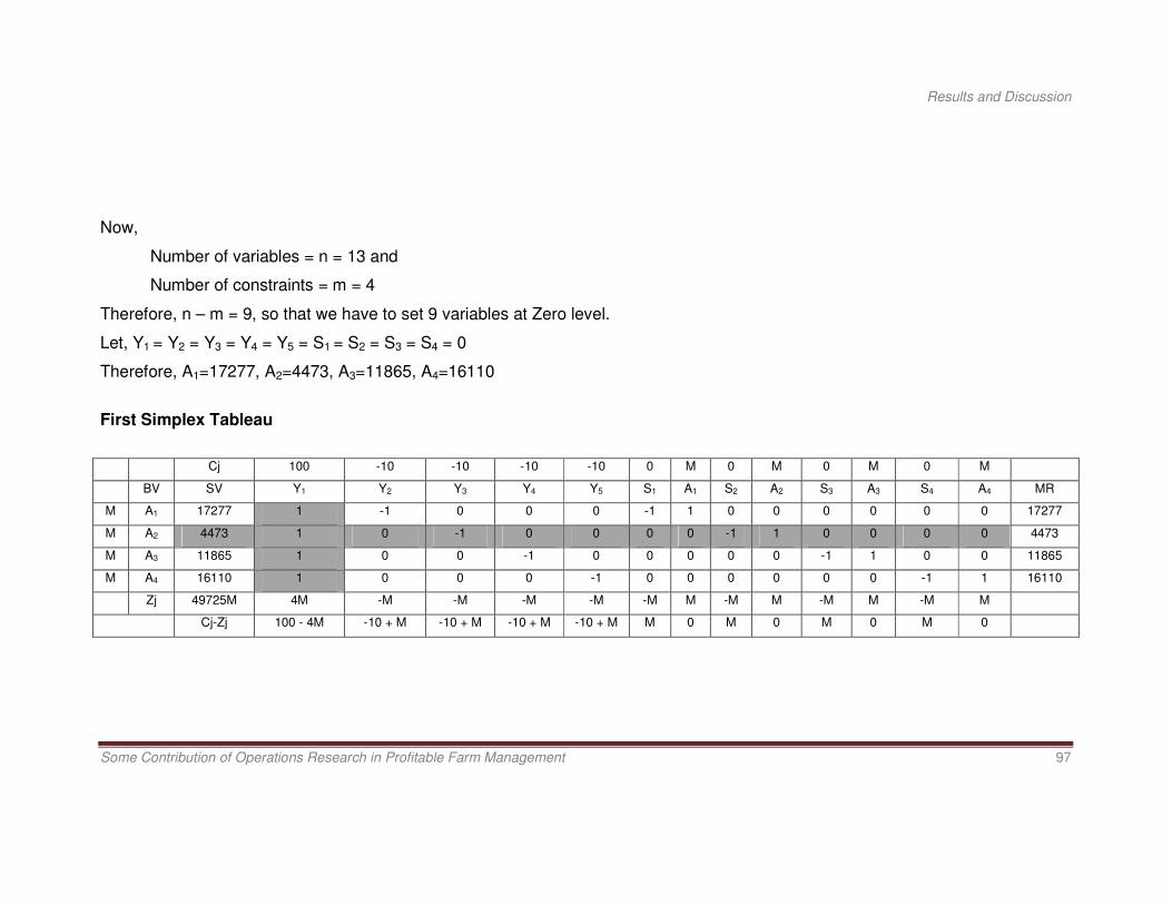
Now,
Number of variables = n = 13 and
Number of constraints = m = 4
Therefore, n – m = 9, so that we have to set 9 variables at Zero level.
Let, Y1 = Y2 = Y3 = Y4 = Y5 = S1 = S2 = S3 = S4 = 0
Therefore, A1=17277, A2=4473, A3=11865, A4=16110
First Simplex Tableau
Cj 100 -10 -10 -10 -10 0 M 0 M 0 M 0 M
BV SV Y1 Y2 Y3 Y4 Y5 S1 A1 S2 A2 S3 A3 S4 A4 MR
M A1 17277 1 -1 0 0 0 -1 1 0 0 0 0 0 0 17277
M A2 4473 1 0 -1 0 0 0 0 -1 1 0 0 0 0 4473
M A3 11865 1 0 0 -1 0 0 0 0 0 -1 1 0 0 11865
M A4 16110 1 0 0 0 -1 0 0 0 0 0 0 -1 1 16110
Zj 49725M 4M -M -M -M -M -M M -M M -M M -M M
Cj-Zj 100 - 4M -10 + M -10 + M -10 + M -10 + M M 0 M 0 M 0 M 0

Results and Discussion
Some Contribution of Operations Research in Profitable Farm Management 98
As the presence of the -ve value in Index Row Cj – Zj, it shows that the solution is not optimum. Now replace A2 by Y1, hence the
Second Simplex Tableau
Cj 100 -10 -10 -10 -10 0 M 0 M 0 M 0 M
BV SV Y1 Y2 Y3 Y4 Y5 S1 A1 S2 A2 S3 A3 S4 A4 MR
M A1 12804 0 -1 1 0 0 -1 1 1 -1 0 0 0 0 12804
100 Y1 4473 1 0 -1 0 0 0 0 -1 1 0 0 0 0
M A3 7392 0 0 1 -1 0 0 0 1 -1 -1 1 0 0 7392
M A4 11637 0 0 1 0 -1 0 0 1 -1 0 0 -1 1 11637
Zj 447300+31833M 100 -M -100+3M -M -M -M M -100+3M 100-3M -M M -M M
Cj-Zj 0 -10 + M 90-3M -10 + M -10 + M M 0 100-3M 100+4M M 0 M 0
Here, presence of the -ve value in Index Row Cj – Zj, so again Replace A3 by Y3, so that the Third Simplex Tableau as
Cj 100 -10 -10 -10 -10 0 M 0 M 0 M 0 M
BV SV Y1 Y2 Y3 Y4 Y5 S1 A1 S2 A2 S3 A3 S4 A4 MR
M A1 5412 0 -1 0 1 0 -1 1 0 0 1 -1 0 0 5412
100 Y1 11865 1 0 0 -1 0 0 0 0 0 -1 1 0 0
-10 Y3 7392 0 0 1 -1 0 0 0 1 -1 -1 1 0 0
M A4 4245 0 0 0 1 -1 0 0 0 0 1 -1 -1 1 4245
Zj 1112580+9657M 100 -M -10 -90+2M -M -M M -10 10 -90+2M 90-2M -M M
Cj-Zj 0 -10 + M 0 80-2M -10 + M M 0 10 -10+M 90-2M 90+3M M 0

Results and Discussion
Some Contribution of Operations Research in Profitable Farm Management 99
Again here the presence of the -ve value in Index Row Cj – Zj, so replace A4 by Y4, therefore the Fourth Simplex Tableau as
Cj 100 -10 -10 -10 -10 0 M 0 M 0 M 0 M
BV SV Y1 Y2 Y3 Y4 Y5 S1 A1 S2 A2 S3 A3 S4 A4 MR
M A1 1167 0 -1 0 0 1 -1 1 0 0 0 0 0 0 1167
100 Y1 16110 1 0 0 0 -1 0 0 0 0 0 0 0 0
-10 Y3 11637 1 0 1 0 -1 0 0 1 -1 0 0 0 0
-10 Y4 4245 0 0 0 1 -1 0 0 0 0 1 -1 -1 1
Zj 1452180+1167M 90 -M -10 -10 80+M -M M -10 10 -10 10 10 -10
Cj-Zj 10 -10 + M 0 0 -90- M M 0 10 -10+M 10 -10+M -10 10+M
Here, presence of the -ve value in Index Row Cj – Zj, so again Replace A1 by Y5, so that the Fifth Simplex Tableau as
Cj 100 -10 -10 -10 -10 0 M 0 M 0 M 0 M
BV SV Y1 Y2 Y3 Y4 Y5 S1 A1 S2 A2 S3 A3 S4 A4 MR
-10 Y5 1167 0 -1 0 0 1 -1 1 0 0 0 0 0 0
100 Y1 17277 1 -1 0 0 0 -1 1 0 0 0 0 0 0
-10 Y3 12804 1 -1 1 0 0 -1 1 1 -1 0 0 0 0
-10 Y4 5412 0 -1 0 1 0 -1 1 0 0 1 -1 -1 1
Zj 1533870 90 -70 -10 -10 -10 -70 70 -10 10 -10 10 10 -10
Cj-Zj 10 60 0 0 0 70 -70+M 10 -10+M 10 -10+M -10 10+M

Results and Discussion
Some Contribution of Operations Research in Profitable Farm Management 100
Decision: Finally, there is the presence of +ve value in Index Row Cj – Zj of Fourth Simplex Tableau, which shows that the
solution is optimum. Thus, the optimal solution by Dual Simplex Method is Max Z= 1533870 with X1=70, X2=10, X3=10
and X4=10
5.6.2.2.3 Solution by Two Phase Simplex Method
For converting inequality to equality, we have to add slack variable S1 in first constraint; subtract surplus variable S2 and add
artificial variable A1 in second constraint, subtract surplus variable S3 and add artificial variable A2 in third constraint, subtract
surplus variable S4 and add artificial variable A3 in fourth constraint and subtract surplus variable S5 and add artificial variable A4 in
fifth constraint
The model converted into equality from inequality which is given by
Max Z = 17277 X1 + 4473 X2 + 11865 X3 + 16110 X4 + 0S1 – 0S2 + MA1 – 0S3 + MA2 – 0S4 + MA3 – 0S5 + MA4
Subject to the constraints:
X1 + X2 + X3 + X4 + S1 = 100
X1 – S2 + A1 = 10
X2 – S3 + A2 = 10
X3– S4 + A3 = 10
X4 – S5 + A4 = 10

Results and Discussion
Some Contribution of Operations Research in Profitable Farm Management 101
Now,
Number of variables = n = 13 and
Number of constraints = m = 5.
Therefore, n – m = 8
so that we have to set 8 variables at Zero level.
Let, X1 = X2 = X3 = X4 = S2 = S3 = S4 = S5 =0
Therefore, S1 = 100, A1=10, A2=10, A3=10, A4=10
Assign 0 coefficient to V Xi and V Si and assign -1 coefficient to V Ai in this Two Phase Simplex method.
Phase – I, First Simplex Tableau
Cj 0 0 0 0 0 0 -1 0 -1 0 -1 0 -1
BV SV X1 X2 X3 X4 S1 S2 A1 S3 A2 S4 A3 S5 A4 MR
0 S1 100 1 1 1 1 1 0 0 0 0 0 0 0 0 100
-1 A1 10 1 0 0 0 0 -1 1 0 0 0 0 0 0 10
-1 A2 10 0 1 0 0 0 0 0 -1 1 0 0 0 0
-1 A3 10 0 0 1 0 0 0 0 0 0 -1 1 0 0
-1 A4 10 0 0 0 1 0 0 0 0 0 0 0 -1 1
Zj -40 -1 -1 -1 -1 0 1 -1 1 -1 1 -1 1 -1
Cj-Zj 1 1 1 1 0 -1 0 -1 0 -1 0 -1 0

Results and Discussion
Some Contribution of Operations Research in Profitable Farm Management 102
As the presence of the +ve value in Index Row Cj – Zj, it shows that the solution is not optimum. Now replace A1 by X1, hence the
Second Simplex Tableau
Cj 0 0 0 0 0 0 -1 0 -1 0 -1 0 -1
BV SV X1 X2 X3 X4 S1 S2 A1 S3 A2 S4 A3 S5 A4 MR
0 S1 90 0 1 1 1 1 1 0 0 0 0 0 0 90
0 X1 10 1 0 0 0 0 -1 0 0 0 0 0 0
-1 A2 10 0 1 0 0 0 0 -1 1 0 0 0 0 10
-1 A3 10 0 0 1 0 0 0 0 0 -1 1 0 0
-1 A4 10 0 0 0 1 0 0 0 0 0 0 -1 1
Zj -30 0 -1 -1 -1 0 0 1 -1 1 -1 1 -1
Cj-Zj 0 1 1 1 0 0 -1 0 -1 0 -1 0
Here, presence of the +ve value in Index Row Cj – Zj, so again Replace A2 by X2, so that the Third Simplex Tableau as
Cj 0 0 0 0 0 0 -1 0 -1 0 -1 0 -1
BV SV X1 X2 X3 X4 S1 S2 A1 S3 A2 S4 A3 S5 A4 MR
0 S1 80 0 0 1 1 1 1 1 0 0 0 0 80
0 X1 10 1 0 0 0 0 -1 0 0 0 0 0
0 X2 10 0 1 0 0 0 0 -1 0 0 0 0
-1 A3 10 0 0 1 0 0 0 0 -1 1 0 0 10
-1 A4 10 0 0 0 1 0 0 0 0 0 -1 1
Zj -20 0 0 -1 -1 0 0 0 1 -1 1 -1
Cj-Zj 0 0 1 1 0 0 0 -1 0 -1 0

Results and Discussion
Some Contribution of Operations Research in Profitable Farm Management 103
Again here the presence of the +ve value in Index Row Cj – Zj, so replace A3 by X3, therefore the Fourth Simplex Tableau as
Cj 0 0 0 0 0 0 -1 0 -1 0 -1 0 -1
BV SV X1 X2 X3 X4 S1 S2 A1 S3 A2 S4 A3 S5 A4 MR
0 S1 70 0 0 0 1 1 1 1 1 0 0 70
0 X1 10 1 0 0 0 0 -1 0 0 0 0
0 X2 10 0 1 0 0 0 0 -1 0 0 0
0 X3 10 0 0 1 0 0 0 0 -1 0 0
-1 A4 10 0 0 0 1 0 0 0 0 -1 1 10
Zj -10 0 0 0 -1 0 0 0 0 1 -1
Cj-Zj 0 0 0 1 0 0 0 0 -1 0
Here presence of the +ve value in Index Row Cj – Zj, therefore, replace A4 by X4, thereby the Fifth Simplex Tableau as
Cj 0 0 0 0 0 0 -1 0 -1 0 -1 0 -1
BV SV X1 X2 X3 X4 S1 S2 A1 S3 A2 S4 A3 S5 A4 MR
0 S1 60 0 0 0 0 1 1 1 1 1
0 X1 10 1 0 0 0 0 -1 0 0 0
0 X2 10 0 1 0 0 0 0 -1 0 0
0 X3 10 0 0 1 0 0 0 0 -1 0
0 X4 10 0 0 0 1 0 0 0 0 -1
Zj 0 0 0 0 0 0 0 0 0 0
Cj-Zj 0 0 0 0 0 0 0 0 0

Results and Discussion
Some Contribution of Operations Research in Profitable Farm Management 104
Here, all entry of Index Row Cj – Zj is Zero and no artificial variable is present, so the solution is optimum for Phase – I method.
Now converting it into Phase – II method thereby the Phase – II, Sixth Simplex Tableau as
Cj 17277 4473 11865 16110 0 0 0 0 0
BV SV X1 X2 X3 X4 S1 S2 S3 S4 S5 MR
0 S1 60 0 0 0 0 1 1 1 1 1 60
17277 X1 10 1 0 0 0 0 -1 0 0 0
4473 X2 10 0 1 0 0 0 0 -1 0 0
11865 X3 10 0 0 1 0 0 0 0 -1 0
16110 X4 10 0 0 0 1 0 0 0 0 -1
Zj 497250 17277 4473 11865 16110 0 -17277 -4473 -11865 -16110
Cj-Zj 0 0 0 0 0 17277 4473 11865 16110
As presence of the +ve value in Index Row Cj – Zj, replace S1 by S2, hence the Seventh Simplex Tableau as
Cj 17277 4473 11865 16110 0 0 0 0 0
BV SV X1 X2 X3 X4 S1 S2 S3 S4 S5 MR
0 S2 60 0 0 0 0 1 1 1 1 1
17277 X1 70 1 0 0 0 1 0 1 1 1
4473 X2 10 0 1 0 0 0 0 -1 0 0
11865 X3 10 0 0 1 0 0 0 0 -1 0
16110 X4 10 0 0 0 1 0 0 0 0 -1
Zj 1533870 17277 4473 11865 16110 17277 0 12764 5412 1167
Cj-Zj 0 0 0 0 -17277 0 -12764 -5412 -1167

Results and Discussion
Some Contribution of Operations Research in Profitable Farm Management 105
Decision: Finally, there is the presence of –ve value in Index Row Cj – Zj of Seventh Simplex Tableau, which shows that the
solution is optimum. Thus, the optimal solution by Two Phase Simplex Method is Max Z= 1533870 with X1=70, X2=10,
X3=10 and X4=10
The results by all the three LPP techniques applied manually i.e. Big M (Penalty), Dual and Two Phase methods were
identical and presented in the Table 5.2.
Table 5.2 Result of four crops selection by LPP Technique
Particular Result by Simplex method
Big M Dual Two Phase
Max. Profit = Rs. 1533870 Rs. 1533870 Rs. 1533870
X1, Wheat (irri) crop area = 70 ha 70 ha 70 ha
X2, Wheat (unirri) crop area = 10 ha 10 ha 10 ha
X3, Jowar crop area = 10 ha 10 ha 10 ha
X4, Pigeon pea crop area = 10 ha 10 ha 10 ha

Results and Discussion
Some Contribution of Operations Research in Profitable Farm Management 106
5.6.2.3 Comparison between ICT and LP model results
It was found from Fig. 5.6 and Table 5.2 that both the tool applied to
the problem of farmer ABC for selection of the crops B1 (Wheat Irrigated), B2
(Wheat un irrigated), B3 (Jowar) and B4 (Pigeon pea) crops in the Rabi
season was identical i.e. profit was Rs. Rs. 1533870 with land allocation as
70, 10, 10 and 10 ha respectively to each crop which also proved that the
developed ICT is validated.
5.6.3 Three crops per season
Suppose a ABC farmer (Village: XYZ) wanted to select the crops to be
grown under 100 ha area for the Zaid season from the Table 3.4 as C1
(Bajra), C2 (Paddy) and C3 (Groundnut) crops.
5.6.3.1 Results from developed ICT
The three crop selection and available land for the Zaid season was
used as input to the ICT and it showed the result as shown in Fig. 5.7
Fig. 5.7 Result of three crops selection by ICT

Results and Discussion
Some Contribution of Operations Research in Profitable Farm Management 107
5.6.3.2 Results from LP model
Now for the validation of that result obtained from ICT as in Fig. 5.7,
the same crop selection was applied to the LP model as described in eq. 3.1
with the constraints as eq. 3.2 to 3.7 and solved by Big M (Penalty), Dual and
Two Phase Simplex method as followed considering the profit of each crop
selected as below.
Problem Statement:
Suppose a farmer wants to grow Bajra, Paddy and Groundnut crops in the
Zaid season. Profit in Rs. per ha from each crop are 12114, 39625 and 28015
respectively. The farmer has available land as 100 ha and he wants to
allocate at least 10 % of land for each crop. This statement has been made
from Table 3.4.
Mathematical Formulation of LPP:
Primal Problem Max Z = 12114 A31 + 39625 A32 + 28015 A33
= 12114 X1 + 39625 X2 + 28015 X3
Subject to the constraints:
X1 + X2 + X3 < 100
X1 > 10
X2 > 10
X3 > 10
X1, X2, X3 > 0
Sr. No. Crops Profit (Rs/ha)
A31 Bajra 12114
A32 Paddy 39625
A33 Groundnut 28015

Results and Discussion
Some Contribution of Operations Research in Profitable Farm Management 108
5.6.3.2.1 Solution by Big M (Penalty) Simplex Method
For converting inequality to equality, we have to add slack variable S1 in first constraint, subtract surplus variable S2 and add
artificial variable A1 in second constraint, subtract surplus variable S3 and add artificial variable A2 in third constraint, subtract
surplus variable S4 and add artificial variable A3 in fourth constraint i.e.
X1 + X2 + X3 + S1 = 100
X1 – S2 + A1 = 10
X2 – S3 + A2 = 10
X3 – S4 + A3 = 10
Now,
Number of variables = n = 10 and
Number of constraints = m = 4
Therefore, n – m = 6
So that we have to set 10 variables at Zero level. Let, X1 = X2 = X3 = S2 = S3 = S4 = 0
Therefore,
S1=100
A1=10
A2=10
A3=10

Results and Discussion
Some Contribution of Operations Research in Profitable Farm Management 109
First Simplex Tableau
Cj 12114 39625 28015 0 0 -M 0 -M 0 -M
BV SV X1 X2 X3 S1 S2 A1 S3 A2 S4 A3 MR
0 S1 100 1 1 1 1 0 0 0 0 0 0 100
-M A1 10 1 0 0 0 -1 1 0 0 0 0
-M A2 10 0 1 0 0 0 0 -1 1 0 0 10
-M A3 10 0 0 1 0 0 0 0 0 -1 1
Zj -30M -M -M -M 0 M -M M -M M -M
Cj-Zj 12114 + M 39625 + M 28015 +M 0 -M 0 -M 0 -M 0
As the presence of the +ve value in Index Row Cj – Zj, it shows that the solution is not optimum. Now replace A2 by X2, hence the
Second Simplex Tableau
Cj 12114 39625 28015 0 0 -M 0 -M 0 -M
BV SV X1 X2 X3 S1 S2 A1 S3 A2 S4 A3 MR
0 S1 90 1 0 1 1 0 0 1 -1 0 0 90
-M A1 10 1 0 0 0 -1 1 0 0 0 0
39625 X2 10 0 1 0 0 0 0 -1 1 0 0
-M A3 10 0 0 1 0 0 0 0 0 -1 1 10
Zj 396250-20M -M 39625 -M 0 M -M -39625 39625 M -M
Cj-Zj 12114 + M 0 28015 +M 0 -M 0 39625 -39625-M -M 0

Results and Discussion
Some Contribution of Operations Research in Profitable Farm Management 110
Here, presence of the +ve value in Index Row Cj – Zj, so again Replace A3 by X3, so that the Third Simplex Tableau as
Cj 12114 39625 28015 0 0 -M 0 -M 0 -M
BV SV X1 X2 X3 S1 S2 A1 S3 A2 S4 A3 MR
0 S1 80 1 0 0 1 0 0 1 -1 1 -1 80
-M A1 10 1 0 0 0 -1 1 0 0 0 0 10
39625 X2 10 0 1 0 0 0 0 -1 1 0 0
28015 X3 10 0 0 1 0 0 0 0 0 -1 1
Zj 676400-10M -M 39625 28015 0 M -M -39625 39625 -28015 28015
Cj-Zj 12114 + M 0 0 0 -M 0 39625 -39625-M 28015 -28015-M
Again here the presence of the +ve value in Index Row Cj – Zj, so replace A1 by X1, therefore the Fourth Simplex Tableau as
Cj 12114 39625 28015 0 0 -M 0 -M 0 -M
BV SV X1 X2 X3 S1 S2 A1 S3 A2 S4 A3 MR
0 S1 70 0 0 0 1 1 -1 1 -1 1 -1 70
12114 X1 10 1 0 0 0 -1 1 0 0 0 0
39625 X2 10 0 1 0 0 0 0 -1 1 0 0
28015 X3 10 0 0 1 0 0 0 0 0 -1 1
Zj 797540 12114 39625 28015 0 -12114 12114 -39625 39625 -28015 28015
Cj-Zj 0 0 0 0 12114 12114-M 39625 39625-M 28015 28015-M
Results and Discussion
Some Contribution of Operations Research in Profitable Farm Management 111
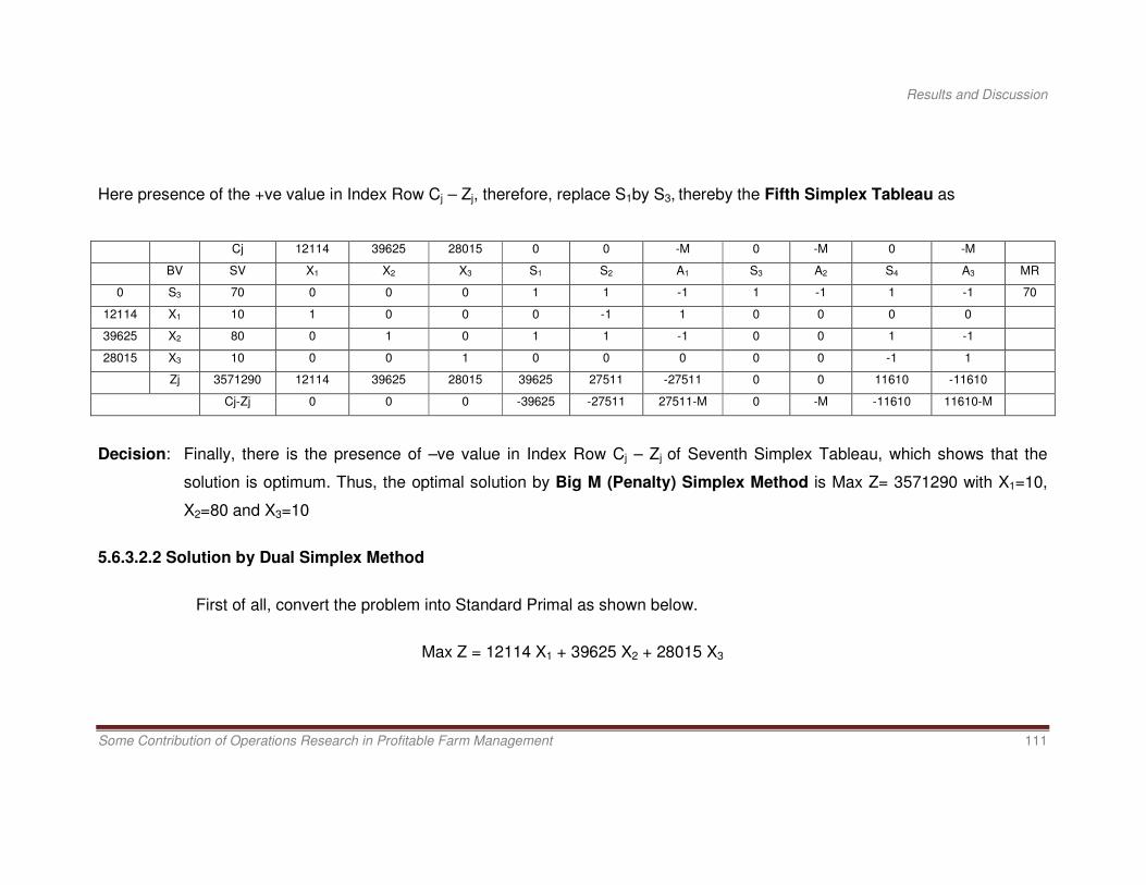
Here presence of the +ve value in Index Row Cj – Zj, therefore, replace S1by S3, thereby the Fifth Simplex Tableau as
Cj 12114 39625 28015 0 0 -M 0 -M 0 -M
BV SV X1 X2 X3 S1 S2 A1 S3 A2 S4 A3 MR
0 S3 70 0 0 0 1 1 -1 1 -1 1 -1 70
12114 X1 10 1 0 0 0 -1 1 0 0 0 0
39625 X2 80 0 1 0 1 1 -1 0 0 1 -1
28015 X3 10 0 0 1 0 0 0 0 0 -1 1
Zj 3571290 12114 39625 28015 39625 27511 -27511 0 0 11610 -11610
Cj-Zj 0 0 0 -39625 -27511 27511-M 0 -M -11610 11610-M
Decision: Finally, there is the presence of –ve value in Index Row Cj – Zj of Seventh Simplex Tableau, which shows that the
solution is optimum. Thus, the optimal solution by Big M (Penalty) Simplex Method is Max Z= 3571290 with X1=10,
X2=80 and X3=10
5.6.3.2.2 Solution by Dual Simplex Method
First of all, convert the problem into Standard Primal as shown below.
Max Z = 12114 X1 + 39625 X2 + 28015 X3

Results and Discussion
Some Contribution of Operations Research in Profitable Farm Management 112
Subject to the constraints:
X1 + X2 + X3 < 100
-X1 < 10
-X2 < 10
-X3 < 10
X1, X2, X3 > 0
The dual of given Standard Primal, Min Z = 100Y1 – 10Y2 – 10Y3 – 10Y4
Subject to the constraints:
Y1 – Y2 > 12114
Y1 – Y3 > 39625
Y1 – Y4 > 28015
Y1, Y2, Y3, Y4 > 0
For converting inequality to equality, we have to subtract surplus variable S1 and add artificial variable A1 in first constraint,
subtract surplus variable S2 and add artificial variable A2 in second constraint and subtract surplus variable S3 and add artificial
variable A3 in third constraint.
Therefore,
Min Z = 100Y1 – 10Y2 – 10Y3 – 10Y4 – 0S1 + MA1 – 0S2 + MA2 – 0S3 + MA3

Results and Discussion
Some Contribution of Operations Research in Profitable Farm Management 113
Subject to the constraints:
Y1 –Y2– S1 + A1 = 12114
Y1 –Y3– S2 + A2 = 39625
Y1 –Y4– S3 + A3 = 28015
Now,
Number of variables = n = 10 and
Number of constraints = m = 3
Therefore, n – m = 7, so that we have to set 7 variables at Zero level.
Let, Y1 = Y2 = Y3 = Y4 = S1 = S2 = S3 = 0
Therefore, A1=12114, A2=39625, A3=28015
First Simplex Tableau
Cj 100 -10 -10 -10 0 M 0 M 0 M
BV SV Y1 Y2 Y3 Y4 S1 A1 S2 A2 S3 A3 MR
M A1 12114 1 -1 0 0 -1 1 0 0 0 0 12114
M A2 39625 1 0 -1 0 0 0 -1 1 0 0 39625
M A3 28015 1 0 0 -1 0 0 0 0 -1 1 28015
Zj 797544M 3M -M -M -M -M M -M M -M M
Cj-Zj 100 - 3M -10 + M -10 + M -10 + M M 0 M 0 M 0

Results and Discussion
Some Contribution of Operations Research in Profitable Farm Management 114
As the presence of the -ve value in Index Row Cj – Zj, it shows that the solution is not optimum. Now replace A1 by Y1, hence the
Second Simplex Tableau
Cj 100 -10 -10 -10 0 M 0 M 0 M
BV SV Y1 Y2 Y3 Y4 S1 A1 S2 A2 S3 A3 MR
100 Y1 12114 1 -1 0 0 -1 1 0 0 0 0 -
M A2 27511 0 1 -1 0 1 -1 -1 1 0 0 27511
M A3 15901 10 1 0 -1 1 -1 0 0 -1 1 15901
Zj 1211400 + 43412M 100 -100 + 2M -M -M -100 + 2M -100 - 2M -M M -M M
Cj-Zj 0 90 - 2M -10 + M -10 + M 100 - 2M -100 + 3M M 0 M 0
Here, presence of the -ve value in Index Row Cj – Zj, so again Replace A3 by Y2, so that the Third Simplex Tableau as
Cj 100 -10 -10 -10 0 M 0 M 0 M
BV SV Y1 Y2 Y3 Y4 S1 A1 S2 A2 S3 A3 MR
100 Y1 28015 1 0 0 -1 0 0 0 0 -1 1 -
M A2 11610 0 0 -1 1 0 0 -1 1 1 -1 11610
-10 Y2 15901 0 1 0 -1 1 -1 0 0 -1 1 -
Zj 2642490 + 11610M 100 -10 -M -90 + M -10 -10 -M M -90 + M 90 - M
Cj-Zj 0 0 -10 + M 80 - M 10 10 + M M 0 90 - M -90 + 2M

Results and Discussion
Some Contribution of Operations Research in Profitable Farm Management 115
Again here the presence of the -ve value in Index Row Cj – Zj, so replace A2 by Y4, therefore the Fourth Simplex Tableau as
Cj 100 -10 -10 -10 0 M 0 M 0 M
BV SV Y1 Y2 Y3 Y4 S1 A1 S2 A2 S3 A3 MR
100 Y1 39625 1 0 -1 0 0 0 -1 1 0 0 -
-10 Y4 11610 0 0 -1 1 0 0 -1 1 1 -1 -
-10 Y3 27511 0 1 -1 0 1 -1 -1 1 0 0 -
Zj 3571290 100 -10 -80 -10 -10 10 -80 80 -10 10
Cj-Zj 0 0 70 0 10 M -10 80 M -80 10 M -10
Decision: Finally, there is the presence of +ve value in Index Row Cj – Zj of Fourth Simplex Tableau, which shows that the
solution is optimum. Thus, the optimal solution by Dual Simplex Method is Max Z= 3571290 with X1=10, X2=80 and
X3=10
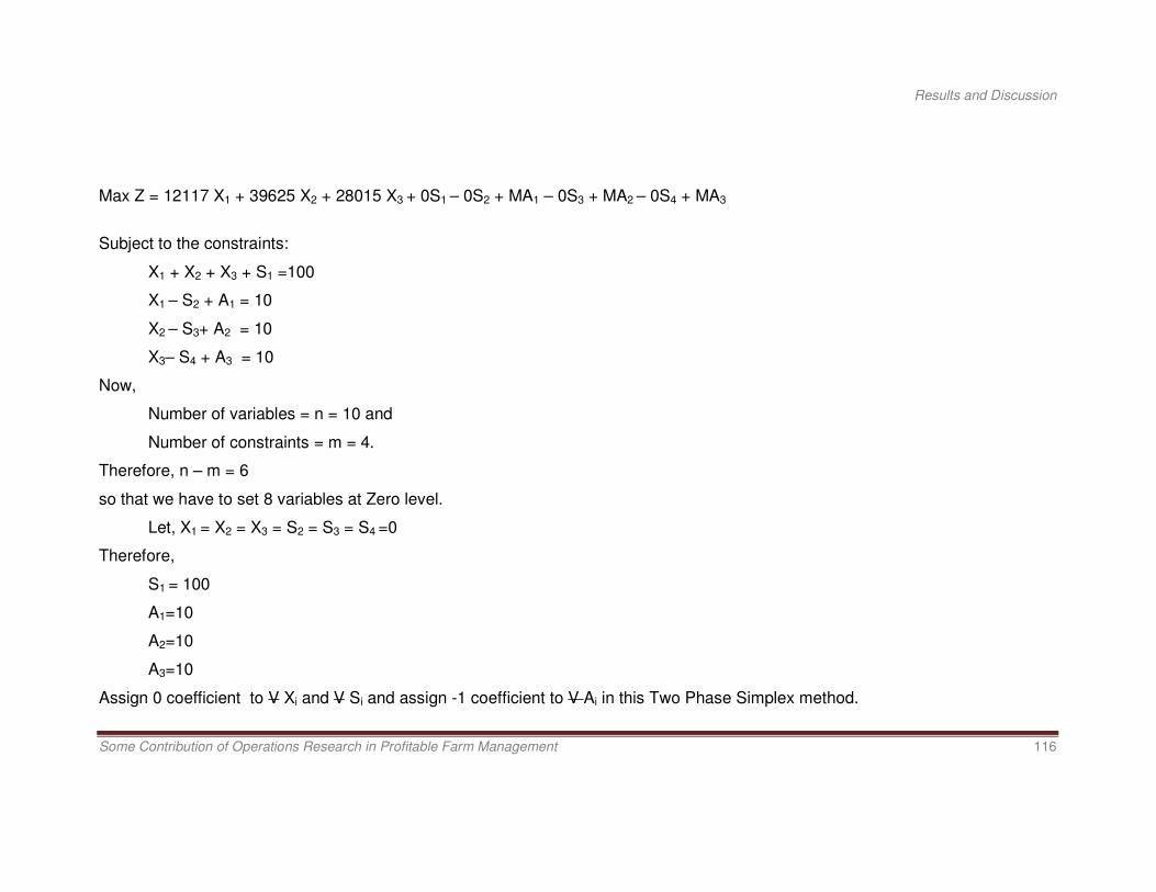
5.6.3.2.3 Solution by Two Phase Simplex Method
For converting inequality to equality, we have to add slack variable S1 in first constraint; subtract surplus variable S2 and add
artificial variable A1 in second constraint, subtract surplus variable S3 and add artificial variable A2 in third constraint and subtract
surplus variable S4 and add artificial variable A3 in third constraint
The model converted into equality from inequality which is given by
Results and Discussion
Some Contribution of Operations Research in Profitable Farm Management 116
Max Z = 12117 X1 + 39625 X2 + 28015 X3 + 0S1 – 0S2 + MA1 – 0S3 + MA2 – 0S4 + MA3
Subject to the constraints:
X1 + X2 + X3 + S1 =100
X1 – S2 + A1 = 10
X2 – S3+ A2 = 10
X3– S4 + A3 = 10
Now,
Number of variables = n = 10 and
Number of constraints = m = 4.
Therefore, n – m = 6
so that we have to set 8 variables at Zero level.
Let, X1 = X2 = X3 = S2 = S3 = S4 =0
Therefore,
S1 = 100
A1=10
A2=10
A3=10
Assign 0 coefficient to V Xi and V Si and assign -1 coefficient to V Ai in this Two Phase Simplex method.

Results and Discussion
Some Contribution of Operations Research in Profitable Farm Management 117
Phase – I, First Simplex Tableau
Cj 0 0 0 0 0 -1 0 -1 0 -1
BV SV X1 X2 X3 S1 S2 A1 S3 A2 S4 A3 MR
0 S1 100 1 1 1 1 0 0 0 0 0 0 100
-1 A1 10 1 0 0 0 -1 1 0 0 0 0 10
-1 A2 10 0 1 0 0 0 0 -1 1 0 0
-1 A3 10 0 0 1 0 0 0 0 0 -1 1
Zj -30 -1 -1 -1 0 1 -1 1 -1 1 -1
Cj-Zj 1 1 1 0 -1 0 -1 0 -1 0
As the presence of the +ve value in Index Row Cj – Zj, it shows that the solution is not optimum. Now replace A1 by X1, hence the
Second Simplex Tableau
Cj 0 0 0 0 0 -1 0 -1 0 -1
BV SV X1 X2 X3 S1 S2 A1 S3 A2 S4 A3 MR
0 S1 90 0 1 1 1 1 1 0 0 0 0 90
0 X1 10 1 0 0 0 -1 1 0 0 0 0
-1 A2 10 0 1 0 0 0 0 -1 1 0 0 10
-1 A3 10 0 0 1 0 0 0 0 0 -1 1
Zj -20 0 -1 -1 0 0 0 1 -1 1 -1
Cj-Zj 0 1 1 0 0 -1 -1 0 -1 0

Results and Discussion
Some Contribution of Operations Research in Profitable Farm Management 118
Here, presence of the +ve value in Index Row Cj – Zj, so again Replace A2 by X2, so that the Third Simplex Tableau as
Cj 0 0 0 0 0 -1 0 -1 0 -1
BV SV X1 X2 X3 S1 S2 A1 S3 A2 S4 A3 MR
0 S1 80 0 0 1 1 1 1 1 -1 0 0 80
0 X1 10 1 0 0 0 -1 1 0 0 0 0
0 X2 10 0 1 0 0 0 0 -1 1 0 0
-1 A3 10 0 0 1 0 0 0 0 0 -1 1 10
Zj -10 0 0 -1 0 0 0 0 0 1 -1
Cj-Zj 0 0 1 0 0 -1 0 -1 -1 0
Again here the presence of the +ve value in Index Row Cj – Zj, so replace A3 by X3, therefore the Fourth Simplex Tableau as
Cj 0 0 0 0 0 -1 0 -1 0 -1
BV SV X1 X2 X3 S1 S2 A1 S3 A2 S4 A3 MR
0 S1 70 0 0 0 1 1 1 1 -1 1 1
0 X1 10 1 0 0 0 -1 1 0 0 0 0
0 X2 10 0 1 0 0 0 0 -1 1 0 0
0 X3 10 0 0 1 0 0 0 0 0 -1 1
Zj 0 0 0 0 0 0 0 0 0 0 0
Cj-Zj 0 0 0 0 0 -1 0 -1 0 -1

Results and Discussion
Some Contribution of Operations Research in Profitable Farm Management 119
Here, all entry of Index Row Cj – Zj is Zero and no artificial variable is present, so the solution is optimum for Phase – I method.
Now converting it into Phase – II method thereby the Phase – II, Fifth Simplex Tableau as
Cj 12114 39625 28015 0 0 0 0
BV SV X1 X2 X3 S1 S2 S3 S4 MR
0 S1 70 0 0 0 1 1 1 1 70
12114 X1 10 1 0 0 0 -1 0 0
39625 X2 10 0 1 0 0 0 -1 0
28015 X3 10 0 0 1 0 0 0 -1
Zj 797540 12114 39625 28015 0 -12114 -39625 -28015
Cj-Zj 0 0 0 0 12114 39625 28015
As presence of the +ve value in Index Row Cj – Zj, replace S1 by S3, hence the Sixth Simplex Tableau as
Cj 12114 39625 28015 0 0 0 0
BV SV X1 X2 X3 S1 S2 S3 S4 MR
0 S3 70 0 0 0 1 1 1 1
12114 X1 10 1 0 0 0 -1 0 0
39625 X2 80 0 1 0 1 1 0 1
28015 X3 10 0 0 1 0 0 0 -1
Zj 3571290 12114 39625 28015 39625 27511 0 11610
Cj-Zj 0 0 0 -39625 -27511 0 -11610

Results and Discussion
Some Contribution of Operations Research in Profitable Farm Management 120
Decision: Finally, there is the presence of –ve value in Index Row Cj – Zj of Seventh Simplex Tableau, which shows that the
solution is optimum. Thus, the optimal solution by Two Phase Simplex Method is Max Z= 3571290 with X1=10, X2=80
and X3=10
The results by all the three LPP techniques applied manually i.e. Big M (Penalty), Dual and Two Phase methods were
identical and presented in the Table 5.3.
Table 5.3 Result of three crops selection by LPP Technique
Particular Result by Simplex method
Big M Dual Two Phase
Max. Profit = Rs. 3571290 Rs. 3571290 Rs. 3571290
X1, Bajra crop area = 10 ha 10 ha 10 ha
X2, Paddy crop area = 80 ha 80 ha 80 ha
X3, Groundnut crop area = 10 ha 10 ha 10 ha
Results and Discussion
Some Contribution of Operations Research in Profitable Farm Management 121
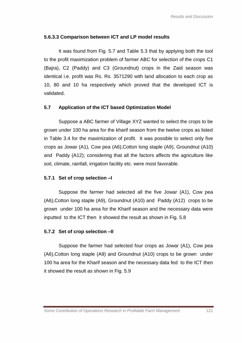
5.6.3.3 Comparison between ICT and LP model results
It was found from Fig. 5.7 and Table 5.3 that by applying both the tool
to the profit maximization problem of farmer ABC for selection of the crops C1
(Bajra), C2 (Paddy) and C3 (Groundnut) crops in the Zaid season was
identical i.e. profit was Rs. Rs. 3571290 with land allocation to each crop as
10, 80 and 10 ha respectively which proved that the developed ICT is
validated.
5.7 Application of the ICT based Optimization Model
Suppose a ABC farmer of Village XYZ wanted to select the crops to be
grown under 100 ha area for the kharif season from the twelve crops as listed
in Table 3.4 for the maximization of profit. It was possible to select only five
crops as Jowar (A1), Cow pea (A6),Cotton long staple (A9), Groundnut (A10)
and Paddy (A12); considering that all the factors affects the agriculture like
soil, climate, rainfall, irrigation facility etc. were most favorable.
5.7.1 Set of crop selection –I
Suppose the farmer had selected all the five Jowar (A1), Cow pea
(A6),Cotton long staple (A9), Groundnut (A10) and Paddy (A12) crops to be
grown under 100 ha area for the Kharif season and the necessary data were
inputted to the ICT then it showed the result as shown in Fig. 5.8
5.7.2 Set of crop selection –II
Suppose the farmer had selected four crops as Jowar (A1), Cow pea
(A6),Cotton long staple (A9) and Groundnut (A10) crops to be grown under
100 ha area for the Kharif season and the necessary data fed to the ICT then
it showed the result as shown in Fig. 5.9

Results and Discussion
Some Contribution of Operations Research in Profitable Farm Management 122
Fig. 5.8 Set of crop selection – I
Fig. 5.9 Set of crop selection – II

Results and Discussion
Some Contribution of Operations Research in Profitable Farm Management 123
5.7.3 Set of crop selection –III
Suppose the farmer had selected only three crops as Jowar (A1), Cow
pea (A6) and Cotton long staple (A9) crops to be grown under 100 ha area
for the Kharif season and the necessary data applied to the ICT then it
showed the result as shown in Fig. 5.10
Fig. 5.10 Set of crop selection –III
5.7.4 Comparison between sets of crop selection
It was found from Fig. 5.8 that the set of crop selection- I showed the
area allocation to each crop and profit as shown in Table 5.4 while Fig. 5.9
showed results of the area allocation to each crop and profit as shown in
Table 5.5. It was found from Fig. 5.10 that the set of crop selection- III showed
the area allocation to each crop and profit as shown in Table 5.6

Results and Discussion
Some Contribution of Operations Research in Profitable Farm Management 124
Table 5.4 Result of set of crop selection – I by ICT
Max. Profit = Rs. 2030160
Jowar crop area = 10 ha
Cow pea crop area = 10 ha
Cotton (LS) crop area = 60 ha
Groundnut crop area = 10 ha
Paddy = 10 ha
Table 5.5 Result of set of crop selection – II by ICT
Max. Profit = Rs. 2104820
Jowar crop area = 10 ha
Cow pea crop area = 10 ha
Cotton (LS) crop area = 70 ha
Groundnut crop area = 10 ha
Table 5.6 Result of set of crop selection – III by ICT
Max. Profit = Rs. 2163170
Jowar crop area = 10 ha
Cow pea crop area = 10 ha
Cotton (LS) crop area = 80 ha
Thus, it was revealed that if the farmer had selected only the three
crops as in Table 5.6 than he would be able to achieve maximum profit of
Rs. 2163170 rather than four (Rs. 2104820) or five crops (Rs. 2030160) for
that season and available land. It was also found that five crops selection
showed the minimum profit compared to other crops selection.