Chapter Twelve

1

CHAPTER TWELVEAggregate Demand in the Open Economy

Chapter Twelve

2

This chapter:

1. The Mundell-Fleming model

2. The small open economy under floating exchange rates

3. The small open economy under fixed exchange rates

Chapter Twelve

3

Assumption 1: The domestic interest rate is equal to the world interest rate (r = r*).Assumption 2: The price level is exogenously fixed since the model is used to analyze the short run (P). This implies that the nominal exchange rate is proportional to the real exchange rate.Assumption 3: The money supply is also set exogenously by the central bank (M).Assumption 4: Our LM* curve will be vertical because the exchange rate does not enter into our LM* equation.

IS*: Y = C(Y-T) + I(r*) + G + NX(e)

LM*: M/P = L (r*,Y)

Start with these two equations:

Chapter Twelve

4

E

Income, Output, Y

Y=EPlanned Expenditure,E = C + I + G + NX

e

Income, Output, Y

e

Net Exports, NX

NX(e) IS*

An increase in the exchange rate, lowers net exports, which shifts planned expenditure downward and lowers income. The IS* curve summarizes these changes in the goods market equilibrium.

An increase in the exchange rate, lowers net exports, which shifts planned expenditure downward and lowers income. The IS* curve summarizes these changes in the goods market equilibrium.

(a) (b)

(c)

Chapter Twelve

5

r

Income, Output, Y

LM

e

Income, Output, Y

LM*

r = r*

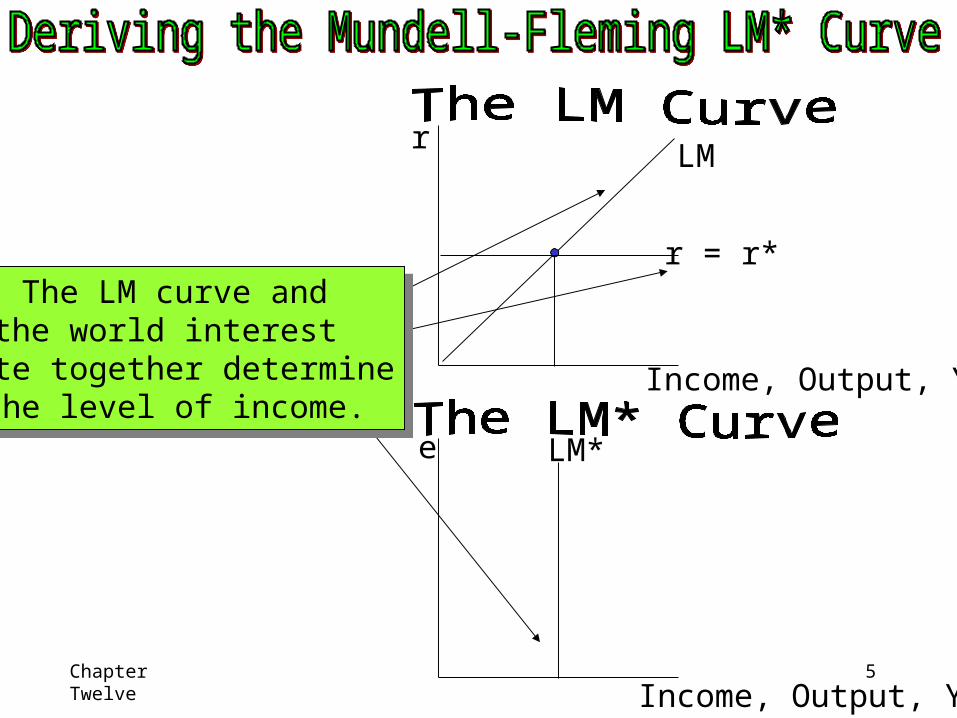
The LM curve andthe world interest

rate together determinethe level of income.

The LM curve andthe world interest

rate together determinethe level of income.

Chapter Twelve

6

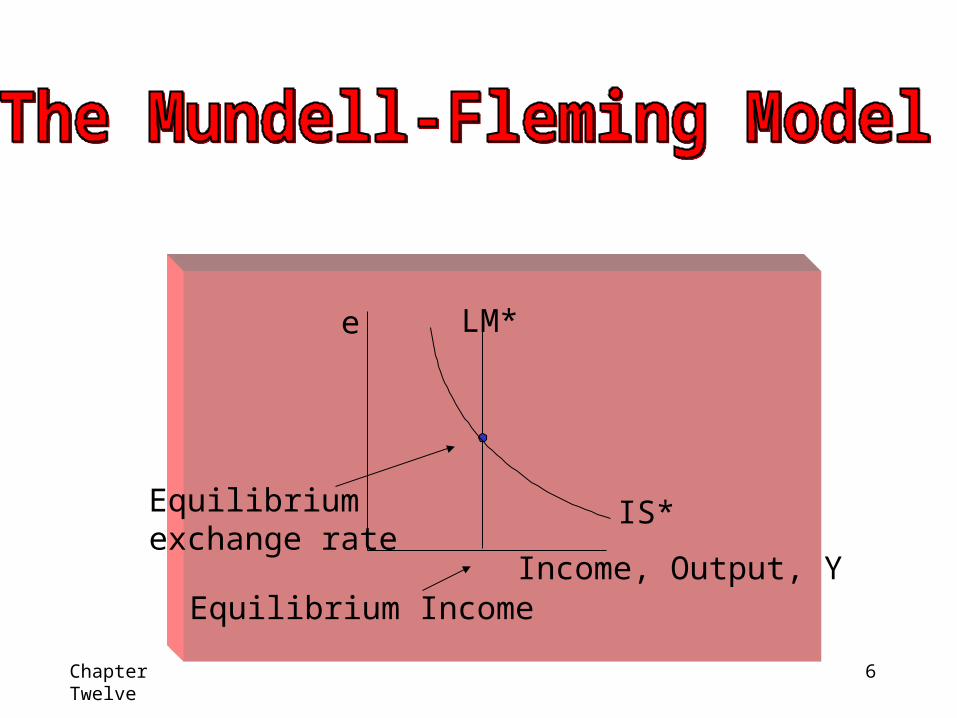
e

Income, Output, Y

LM*

IS*Equilibrium exchange rate

Equilibrium Income

Chapter Twelve

7

Exchange Rates Regimes in Europe, 2004

1. European Monetary Union (fixed exchange rates among themselves, by the adoption of a common currency, the euro): Austria, Belgium, Finland, France, Germany, Greece, Ireland, Italy, Luxembourg, Netherlands, Portugal, Spain

2. Members of the Exchange Rate Mechanism of the European Monetary System: Cyprus, Czech Republic, Denmark, Hungary, Latvia, Malta, Poland, Slovak Republic, Slovenia

Chapter Twelve

8

3. Managed floaters (follow the euro closely, they actively limit the fluctuations of their exchange rates, usually vis-a-vis the euro): Croatia, Macedonia, Norway, Romania, Russia, Sweden, Ukraine

4. Free floaters (largely allow the market to determine their exchange rate): Albania, Iceland, Switzerland, United Kingdom

5. Currency board (they peg to the euro): Estonia, Lithuania, Bosnia-Herzegovina, Bulgaria

Chapter Twelve

9

e

Income, Output, Y

LM*

IS*

e

Income, Output, Y

LM*

IS*IS*'

LM*'

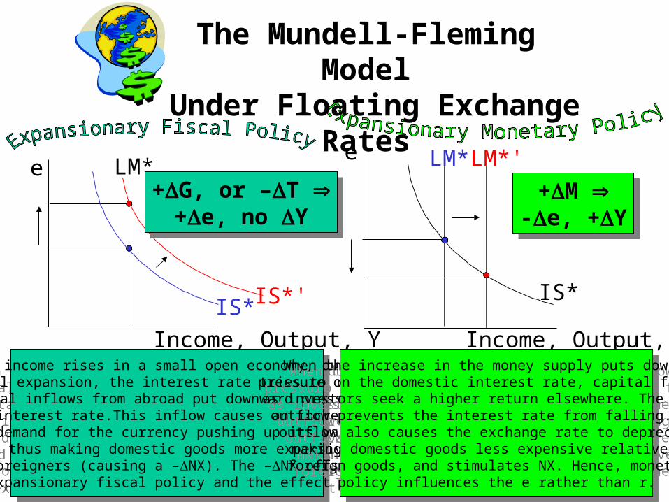
When income rises in a small open economy, due tothe fiscal expansion, the interest rate tries to rise but capital inflows from abroad put downward pressure on the interest rate.This inflow causes an increase in

the demand for the currency pushing up its value and thus making domestic goods more expensive

to foreigners (causing a –NX). The –NX offsets the expansionary fiscal policy and the effect on Y.

When income rises in a small open economy, due tothe fiscal expansion, the interest rate tries to rise but capital inflows from abroad put downward pressure on the interest rate.This inflow causes an increase in

the demand for the currency pushing up its value and thus making domestic goods more expensive

to foreigners (causing a –NX). The –NX offsets the expansionary fiscal policy and the effect on Y.

When the increase in the money supply puts downwardpressure on the domestic interest rate, capital flows outas investors seek a higher return elsewhere. The capital

outflow prevents the interest rate from falling. The outflow also causes the exchange rate to depreciate making domestic goods less expensive relative to

foreign goods, and stimulates NX. Hence, monetary policy influences the e rather than r.

When the increase in the money supply puts downwardpressure on the domestic interest rate, capital flows outas investors seek a higher return elsewhere. The capital

outflow prevents the interest rate from falling. The outflow also causes the exchange rate to depreciate making domestic goods less expensive relative to

foreign goods, and stimulates NX. Hence, monetary policy influences the e rather than r.

+G, or –T +e, no Y

+G, or –T +e, no Y

+M -e, +Y

+M -e, +Y

The Mundell-Fleming Model

Under Floating Exchange Rates

Chapter Twelve

10

The Mundell-Fleming Model Under Fixed Exchange Rates

The goal of the monetary policy of the Central Bank: keep the exchange rate at the announced level.

The essence of a fixed-exchange rate system: the commitment of the Central Bank to allow the money supply to adjust to whatever level will ensure that the equilibrium exchange rate equals the announced exchange rate.

Let’s see how fixing the exchange rate determines the money supply!

ARBITRAGE: the process of buying something such as a commodity or a currency in one place and sell it in another place at the same time.

Chapter Twelve

11

(a) The Equilibrium Exchange Rate is Greater Than the Fixed Exchange Rate

Exchange rate, e

Income, output, Y

IS*

LM1* LM2*

Equilibrium exchange rate

Fixed exchange rate

The Central Bank must increase the money supply

Chapter Twelve

12

(b) The Equilibrium Exchange Rate is Less Than the Fixed Exchange Rate

Exchange rate, e

Income, output, Y

IS*

LM1*LM2*

Equilibrium exchange rate

Fixed exchange rate

The Central Bank must decrease the money supply

Chapter Twelve

13

e

Income, Output, Y

LM*

IS*

e

Income, Output, Y

LM*

IS*IS*'

A fiscal expansion shifts IS* to the right. To maintainthe fixed exchange rate, the Fed must increase themoney supply, thus increasing LM* to the right.

Unlike the case with flexible exchange rates, there is nocrowding out effect on NX due to a higher exchange

rate.

A fiscal expansion shifts IS* to the right. To maintainthe fixed exchange rate, the Fed must increase themoney supply, thus increasing LM* to the right.

Unlike the case with flexible exchange rates, there is nocrowding out effect on NX due to a higher exchange

rate.

If the Fed tried to increase the money supply bybuying bonds from the public, that would put down-

ward pressure on the interest rate. Arbitragers respondby selling the domestic currency to the central bank,

causing the money supply and the LM curveto contract to their initial positions.

If the Fed tried to increase the money supply bybuying bonds from the public, that would put down-

ward pressure on the interest rate. Arbitragers respondby selling the domestic currency to the central bank,

causing the money supply and the LM curveto contract to their initial positions.

+G, or –T + Y+G, or –T + Y

LM*'

+ no Y+ no Y

The Mundell-Fleming Model Under Fixed Exchange Rates

Chapter Twelve

14

Policy in the Mundell-Fleming Model:

A SummaryThe Mundell-Fleming model shows that the effect of almost any economic policy on a small open economy depends on whether the exchange rate is floating or fixed.

The Mundell-Fleming model shows that the power of monetary and fiscal policy to influence aggregate demand depends on the exchange rate regime.

The Mundell-Fleming model shows that the effect of almost any economic policy on a small open economy depends on whether the exchange rate is floating or fixed.

The Mundell-Fleming model shows that the power of monetary and fiscal policy to influence aggregate demand depends on the exchange rate regime.

Chapter Twelve

15

Fixed vs. Floating Exchange Rate Conclusions

The Mundell-Fleming Model: Summary of Policy Effects

Exchange rate regimeFLOATING FIXED

Impact on:Policy

Y e NX Y e NX

Fiscalexpansion

0 0 0

Monetaryexpansion

0 0 0

Importrestriction

0 0 0

Chapter Twelve

16

Fixed vs. Floating Exchange Rate Conclusions

Fixed Exchange Rates

Floating Exchange Rates • Fiscal Policy is Powerful.

• Monetary Policy is Powerless.• Fiscal Policy is Powerless.• Monetary Policy is Powerful.

The Mundell-Fleming model shows that fiscal policy does not influenceaggregate income under floating exchange rates. A fiscal expansioncauses the currency to appreciate, reducing net exports and offsettingthe usual expansionary impact on aggregate demand.

The Mundell –Fleming model shows that monetary policy does not influence aggregate income under fixed exchange rates. Any attempt to expand the money supply is futile, because the money supplymust adjust to ensure that the exchange rate stays at its announced level.

Hint: (Think of floating money.) Hint: (Fixed and Fiscal sound alike).

Chapter Twelve

17

Should Exchange Rates Be Floating or Fixed?

Historically - most economists have favoured a system of floating exchange ratesIn recent years - some advice the return to fixed exchange rates

Arguments for floating exchange rate:- it allows monetary policy to be used for other purposes (stabilizing employment or prices)

Arguments for fixed exchange rates:- exchange rate uncertainty makes international trade more difficult (after Bretton Woods, real and nominal exchange rates became much more volatile than anyone expected)- a commitment to a fixed exchange rate is a way to discipline a nation’s monetary authority and prevent excessive growth in the money supply

Chapter Twelve

18

The choice between floating and fixed exchange rate is more flexible than it may seem at first:

- during periods of fixed exchange rates, countries can change the value of their currency if they notice that maintaining the exchange rate is in conflict with other goals

- during periods of floating exchange rates, countries may use formal or informal targets for the exchange rates when deciding whether to expand or contract the money supply

We rarely observe exchange rates that are completely fixed or completely floating.

The main objective of the central bank: stability of the exchange rate.

Chapter Twelve

19

The higher return will attract funds from the rest of the world, driving the US interest rate back down.

And, if the interest rate were below the world interest rate, domestic residents would lend

abroad to earn a higher return, driving the domestic interest rate back up. In the end, the domestic

interest rate would equal the world interest rate.

What if the domestic interest rate were above the world interest rate?

Chapter Twelve

20

Why doesn’t this logic always apply? There are two reasons why interestrates differ across countries:

1) Country Risk: when investors buy US government bonds, or makeloans to US corporations, they are fairly confident that they will berepaid with interest. By contrast, in some less developed countries, itis plausible to fear that political upheaval may lead to a default on loanrepayments. Borrowers in such countries often have to pay higherinterest rates to compensate lenders for this risk.

2) Exchange Rate Expectations: suppose that people expect the Frenchfranc to fall in value relative to the US dollar. Then loans made in francswill be repaid in a less valuable currency than loans made in dollars. Tocompensate for the expected fall in the French currency, the interest rate in France will be higher than the interest rate in the US.

Chapter Twelve

21

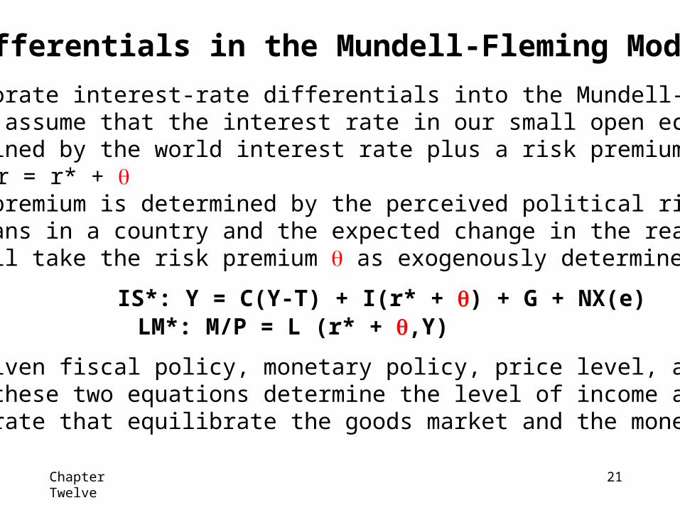
Differentials in the Mundell-Fleming Model

To incorporate interest-rate differentials into the Mundell-Flemingmodel, we assume that the interest rate in our small open economyis determined by the world interest rate plus a risk premium r = r* + The risk premium is determined by the perceived political risk ofmaking loans in a country and the expected change in the real interestrate. We’ll take the risk premium as exogenously determined.

For any given fiscal policy, monetary policy, price level, and riskpremium, these two equations determine the level of income andexchange rate that equilibrate the goods market and the money market.

IS*: Y = C(Y-T) + I(r* + ) + G + NX(e)LM*: M/P = L (r* + ,Y)

Chapter Twelve

22

Now suppose that political turmoil causes the country’s risk premium to rise. The most direct effect is that the domestic interest rate r rises.The higher interest rate has two effects:1) IS* curve shifts to the left, because the higher interest rate reducesinvestment.2) LM* shifts to the right, because the higher interest rate reduces thedemand for money, and this allows a higher level of income for anygiven money supply. These two shifts cause income to rise and thus push down the equilibriumexchange rate on world markets.The important implication: expectations of the exchange rate are partiallyself-fulfilling. For example, suppose that people come to believe that theFrench franc will not be valuable in the future. Investors will place alarger risk premium on French assets: will rise in France. Thisexpectation will drive up French interest rates and will drive down the value of the French franc. Thus, the expectation that a currency will losevalue in the future causes it to lose value today. The next slide will demonstrate the mechanics.

Chapter Twelve

23

e

Income, Output, Y

LM*

IS*

LM*'

IS*'

An Increase in the Risk Premium

An increase in the risk premium associated with a country drives upits interest rate. Because the higher interest rate reduces investment,

the IS* curve shifts to the left. Because it also reduces moneydemand, the LM* curve shifts to the right. Income rises, and the

exchange rate depreciates.

An increase in the risk premium associated with a country drives upits interest rate. Because the higher interest rate reduces investment,

the IS* curve shifts to the left. Because it also reduces moneydemand, the LM* curve shifts to the right. Income rises, and the

exchange rate depreciates.

Is this really is where the economy ends

up? In the next slide, we’ll see that

increases in country risk are not desirable.

Is this really is where the economy ends

up? In the next slide, we’ll see that

increases in country risk are not desirable.

Chapter Twelve

24

There are three reasons why, in practice, such a boom in income does not occur. 1. First, the central bank might want to avoid the large depreciation of the domestic currency and, therefore, may respond by decreasing the money supply M. 2. Second, the depreciation of the domestic currency may suddenly increase the price of domestic goods, causing an increase in the overall price level P. 3. Third, when some event increase the country risk premium, residents of the country might respond to the same event by increasing their demand for money (for any given income and interest rate), because money is often the safest asset available. All three of these changes would tend to shift the LM* curve toward the left, which mitigates the fall in the exchange rate but also tends to depress income.

Chapter Twelve

25

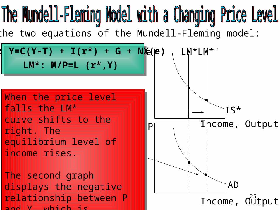
IS*: Y=C(Y-T) + I(r*) + G + NX(e)

LM*: M/P=L (r*,Y)

Recall the two equations of the Mundell-Fleming model:

e

Income, Output,Y

LM*

IS*

LM*'

P

Income, Output,Y

AD

When the price level falls the LM*curve shifts to the right. Theequilibrium level of income rises.

The second graph displays the negative relationship between P and Y, which is summarized by the aggregate demand curve.

When the price level falls the LM*curve shifts to the right. Theequilibrium level of income rises.

The second graph displays the negative relationship between P and Y, which is summarized by the aggregate demand curve.

Chapter Twelve

26

International Financial Crisis: Mexico 1994-1995

• August 1994: a Mexican peso=30 cents• August 1995: a Mexican peso=16cents

What can explain this large fall? COUNTRY RISK is a large part of the story.

Some facts:

- beginning of 1994: NAFTA (North American Free Trade Agreement) reduced trade barriers among USA, Canada and Mexico

- increasing confidence in the Mexican economy

Chapter Twelve

27

- Political changes: a violent uprising in the Chiapas region of Mexico, Luis Donaldo Colosio (the leading presidential candidate) was assasinated

investors started to place a larger risk premium on Mexican assets

Mexico had a fixed exchange rate system at the beginning, the value of peso was not affected (the Mexican Central Bank bought pesos and sold dollars)

But……Mexico’s reserves of foreign currency were too small the government announced a devaluation of the peso at the end of 1994

Chapter Twelve

28

This increased even more the country risk premium (investors became even more distrustful of Mexican policymakers).

Mexican government was unable to pay its debts that were coming due Mexico became in a few months a risky economy with a government on the edge of bankruptcy.

Indebted local firms and banks which had borrowed in foreign currency, mostly dollars, saw their debts double overnight, making them effectively bankrupt.

Chapter Twelve

29

Then……. USA enters. Why? For 3 reasons:

1. To help its neighbor on the south

2. To prevent massive illegal immigration

3. To prevent the investor pessimism regarding Mexico from spreading to other developing countries

Chapter Twelve

30

USA provided loan guarantees for Mexican government debt some of the confidence in the Mexican economy was restored.

Anyway, this was a painful experience for Mexican people, because the country experienced a deep recession as well.

The lesson from this: changes in perceived country risk (political instability) are an important determinant of interest rates and exchange rates in small open economies.

Chapter Twelve

31

Mundell-Fleming ModelFloating exchange ratesFixed exchange rates

Mundell-Fleming ModelFloating exchange ratesFixed exchange rates