chapter three

Chapter 3

Motion of a pointlike particle witha single degree of freedom

3.1 Continuous observables

In this chapter, we study basic quantum physics of the simplest mechanical system: translationalmotion of a pointlike particle with a single degree of freedom. In classical mechanics, this motionis described by two canonical variables, position and momentum. Accordingly, in our quantumtreatment, we introduce two observable operators: position x and momentum p.

In a Hilbert space of finite dimension, we expect (see Ex. 1.76) the set of eigenstates of anyphysical observable to form an orthonormal basis. However, in the present case this rule can beapplied only partially. This is because, although the geometric space containing the particle is one-dimensional, the associated Hilbert space is of infinite dimension: for example, there are infinitelymany position eigenstates |x⟩, and all these eigenstates are incompatible1. Furthermore, positioneigenstates form a continuum: for every real value of x there exists an associated eigenstate |x⟩.The same is true for the momentum observable.

The continuous nature of these observables implies that most mathematical rules (state andoperator decomposition, normalization, basis conversion, etc.) derived for finite-dimension Hilbertspaces have to be modified: summation must be replaced by integration. This is our task for thissection. In order to reproduce these rules in the form that closely resembles those for the discretecase, we need to define a special normalization convention for continuous observable eigenstates.Instead of normalizing these states to one, as we would do in the discrete case [cf. Eq. (1.8)], wewrite:

⟨x| x′⟩ = δ(x− x′); (3.1)

⟨p| p′⟩ = δ(p− p′). (3.2)

This appears strange at first. According to Eq. (3.1), the inner product of the position eigenstate|x⟩ with itself is ⟨x| x⟩ = δ(0), so this state has infinite norm. The same applies to momentumeigenstates. How is this consistent with the First postulate of quantum mechanics, which says thatall physical states must have norm 1? We answer this question by saying that continuous-observableeigenstates are unphysical : it is impossible to set a particle at an absolutely precise location or makeit move at an absolutely precise velocity. Therefore, the First postulate does not apply to thesestates; they are just a mathematical abstraction2. This notwithstanding, all physically realistic

1One may argue that one can also introduce continuous observables in finite-dimensional Hilbert spaces: forexample, the polarization angle of a photon can take on any value from 0 to 180◦. However, this would not be anobservable in the quantum mechanical sense, because the relevant eigenstates are not orthogonal: a photon polarizedat 45◦ is a superposition of the 0◦ and 90◦ polarization states. On the other hand, a particle located at x = 4m is nota superposition of the |x = 3m⟩ and |x = 5m⟩ position eigenstates. A particle’s position is a valid observable while aphoton’s polarization angle is not.

2To treat this matter more rigorously, one introduces a special construction called rigged Hilbert space.

51

52 Quantum Mechanics I

states, which have some uncertainty both in the position and momentum, do have norm one inaccordance with the First postulate.

Any quantum states |ψ⟩ can be decomposed into the basis associated with a continuous-variableobservable according to

|ψ⟩ =∫ +∞

−∞ψ(x) |x⟩ dx. (3.3)

This equation replaces Eq. (1.1) for the decomposition of a state into a discrete basis. The functionψ(x) is called the wavefunction of the state |ψ⟩ in the x-basis (-representation) and is the continuous-observable analog of the column representation of a vector in a Hilbert space of a finite dimension.Taking the adjoint of both sides of Eq. (3.3),

⟨ψ| =∫ +∞

−∞ψ∗(x) ⟨x| dx. (3.4)

we also find that the wavefunction of ⟨ψ| is ψ∗(x).

Exercise 3.1 Show that we can construct the following continuous analogues to important discrete-case relations:

a) Instead of Eq. (1.11), we can writeψ(x) = ⟨x| ψ⟩ ; (3.5)

b) Instead of Eq. (1.31), we can write ∫ +∞

−∞|x⟩⟨x| dx = 1; (3.6)

c) Instead of Eq. (1.9), we can write

⟨ψ1| ψ2⟩ =∫ +∞

−∞ψ∗1(x)ψ2(x)dx; (3.7)

Exercise 3.2 Show that, if the normalization rule were, as in the finite-dimensional case, ⟨x| x′⟩ ={1 if x=x′

0 if x =x′ , the above relations would be invalid.

Exercise 3.3 Show that, for physical states,∫ +∞

−∞|ψ(x)|2dx = 1. (3.8)

Exercise 3.4 Calculate the normalization factor A for the states with the following wavefunctions:

a) a “top-hat function”

ψtop−hat(x) =

{0 if x < a or x > b;A if a ≤ x ≤ b; (3.9)

b) a Gaussian wavefunction

ψGauss(x) = Ae−x2

2d2 . (3.10)

Exercise 3.5 Find the wavefunction of the state of definite position |x0⟩ in the position basis.

As in the discrete case, operators associated with continuous observables are given by

x =

∫ +∞

−∞x |x⟩ ⟨x| dx. (3.11)

3.1. CONTINUOUS OBSERVABLES 53

The operator functions are naturally defined as

f(x) =

∫ +∞

−∞f(x) |x⟩ ⟨x| dx. (3.12)

For an arbitrary operator A, the two-dimensional function

A(x, x′) = ⟨x| A |x′⟩ , (3.13)

is referred to as the operator’s matrix element.As we see below and similarly to the discrete-variable case, the information about the matrix

element ⟨x| A |x′⟩ for all x and x′ is sufficient to reconstruct the operator. More generally, we canperform operations with states and operators represented by one- and two-dimensional functions,respectively, just as we operate with matrices in the discrete case, only replacing summation withintegration.

Exercise 3.6 Show that x |x⟩ = x |x⟩.

Exercise 3.7 Prove that:

a) any operator A can be written as

A =

∫ +∞

−∞

∫ +∞

−∞A(x, x′) |x⟩⟨x′| dx dx′; (3.14)

b) if the operator is a function of x,

⟨ψ| f(x) |ψ⟩ =∫ +∞

−∞ψ∗(x)f(x)ψ(x)dx; (3.15)

c) for any operator A, and any two states |ψ⟩, |ϕ⟩

⟨ϕ| A |ψ⟩ =∫ +∞

−∞

∫ +∞

−∞ϕ∗(x)A(x, x′)ψ(x′)dx dx′; (3.16)

d) the wavefunction of the state A |ψ⟩ is⟨x∣∣∣ A∣∣∣ ψ⟩ =

∫ +∞

−∞A(x, x′)ψ(x′)dx′; (3.17)

e) the wavefunction of the state ⟨ψ| A is⟨ψ∣∣∣ A∣∣∣ x⟩ =

∫ +∞

−∞ψ∗(x′)A(x′, x)dx′; (3.18)

f) matrix elements of an operator A and its adjoint A† are related as

(A†)(x, x′) = A∗(x′, x); (3.19)

g) the product of operators A and B can be written in terms of their “matrices” as⟨x∣∣∣ AB∣∣∣ x′⟩ =

∫ +∞

−∞A(x, x′′)B(x′′, x′)dx′′. (3.20)


Figure 3.1: Approximate measurement of the position by projecting state |ψ⟩ onto a state with a“top-hat” wavefunction.

Let us now reformulate the Second postulate of quantummechanics for measurements in continuous-variable bases. Suppose observable x is measured in quantum state |ψ⟩ with wavefunction ⟨x| ψ⟩ =ψ(x). Acting similarly to the discrete case, we assign value prx = |ψ(x)|2 as the probability toobserve a particular value of x. A subtlety arises, though, because if we associate this (or any otherfinite) probability value to each specific x out of the continuum, the total probability to detect anyx will be infinite. This is not surprising because, as we discussed earlier, eigenstates of the posi-tion operator are unphysical, and so is a projection measurement involving these states. It is eventheoretically not feasible to realize a perfectly precise measurement of the position observable.

As an alternative, let us model the measurement of x project state |ψ⟩ onto the state with a“top-hat” wavefunction (3.9) that takes a constant, non-zero value in the interval between x andx+∆x, where ∆x is arbitrarily small (Fig. 3.1). We find in the first order approximation

⟨ψ| ψtop−hat⟩ =1√∆x

x+∆x∫x

ψ(x)dx ≈√∆xψ(x) (3.21)

and hence the probability to detect state |ψtop−hat⟩ in state |ψ⟩ equals

prx∆x = |⟨ψ| ψtop−hat⟩|2 = |ψ(x)|2∆x. (3.22)

Of course, not all apparata that measure the particle’s position involve projection onto the top-hat function. However, the above result is universally applicable: the probability to detect a particlein state |ψ⟩ within a small interval [x, x + ∆x] is given by Eq. (3.22). Accordingly, the quantityprx = |ψ(x)|2 has the meaning of the probability density associated with the state at position x.

If we apply Eq. (3.22) to find the probability to detect any value of x between −∞ to +∞, wefind unity in accordance with Eq. (3.8). This is not surprising: the particle can with certainty befound somewhere, even though its precise position is not known.

Upon which state |ψ⟩ will project after the measurement? The self-suggesting answer |x⟩ is, aswe discussed, unphysical. Yet it is useful as an approximation for many theoretical applications, aslong as we do not forget to take the normalization issue into account. The more physically realisticanswer will depend on the specifics of the measurement apparatus; generally, one would obtain somesuperposition or statistical mixture of multiple position eigenstates within a certain narrow interval.For example, in the case studied above, the answer is |ψtop−hat⟩.

Closely related to measurements is the notion of the expectation value. Definition 1.26 canbe reformulated for the continuous domain as follows: the expectation value associated with ameasurement of a random continuous variable x with probability density prx is given by

⟨x⟩ =∫ +∞

−∞xprxdx. (3.23)

Under this definition, the expression (1.36) for the quantum expectation value remains the same. Iinvite the reader to verify this independently in the following exercise.

3.2. DE BROGLIE WAVE 55

Exercise 3.8 Show that the expectation value of a continuous observable x [defined as ⟨x⟩ =∫ +∞−∞ xpr(x) dx] in a state |ψ⟩ is given by ⟨x⟩ = ⟨ψ| x |ψ⟩.

Exercise 3.9 Show that the eigenstates of a Hermitian operator corresponding to different eigen-values are orthogonal3.

Table 3.1: Comparative summary of rules for operating with discrete-and continuous-variable bases

discrete basis {|vi⟩} continuous basis {|x⟩}orthonormality ⟨vi| vj⟩ = δij ⟨x| x′⟩ = δ(x− x′)decomposition |ψ⟩ =

∑i

ψi |vi⟩ |ψ⟩ =∫ +∞−∞ ψ(x) |x⟩

of a state ψi = ⟨vi| ψ⟩ ψ(x) = ⟨x| ψ⟩second postulate pri = | ⟨vi| ψ⟩ |2 prx = | ⟨x| ψ⟩ |2

(probability) (probability density)

decomposition Aij =⟨vi

∣∣∣ A∣∣∣ vj⟩ A(x, x′) =⟨x∣∣∣ A∣∣∣ x′⟩

of an operator A =∑i,j

Aij |vi⟩⟨vj | A =∫ +∞−∞

∫ +∞−∞ A(x, x′) |x⟩⟨x′| dxdx′

decomposition of 1 1 =∑i

|vi⟩⟨vi| 1 =∫ +∞−∞ |x⟩⟨x| dx

product of operators (AB)ij =∑k

AikBkj (AB)(x, x′) =∫ +∞−∞ A(x, x′′)B(x′′, x)dx′

3.2 De Broglie wave

In the previous section, we studied the general mathematical machinery for handling the basis ofthe Hilbert space formed by the eigenstates of a continuous observable. Now it is time to bring somephysics into the picture. We begin by postulating the relation between the position and momentumeigenstates:

⟨x| p⟩ = 1√2π~

eipx~ . (3.24)

Relation (3.24) states that the wavefunction of the state with definite momentum is an infinite waveof wavelength

λdB = 2π~/p, (3.25)

which is known as the de Broglie wave. It manifests one of the central concepts of quantum mechanics— wave-particle duality, i.e. the property of all quantum matter to exhibit both particle and wavefeatures.

The de Broglie wave cannot be derived from the quantum mechanics postulates we studied so far.Rather, it is a generalization of a multitude of experimental observations and theoretical insights.The historical path towards the de Broglie wave can be briefly outlined as follows.

In 1900, Max Planck explained the experimentally observed spectrum of blackbody radiationby introducing the quantum of light, now known as the photon4. He found that a good agreementbetween theory and experiment can be obtained if one assumes that the energy of the photon isproportional to the frequency ω of the light wave. The proportionality coefficient, ~, became knownas the Planck constant.

Subsequently, in 1913, Niels Bohr has used the Planck constant in developing his model of theatom, according to which, the electron’s orbital is stable if its angular momentum equals an integernumber of ~. Based on this assumption one can calculate the spectrum of optical transitions ofthe hydrogen atom, which exhibits very good agreement with the experiment. Similarly to Planck’s

3This appears to follow from Ex. 1.76. However, the statement of that Exercise was proven for a Hilbert space ofa finite dimension. In the present Chapter, the dimensions are infinite.

4The term photon has been introduced much later, in 1926, by the physical chemist Gilbert Lewis.


theory of light, Bohr’s model was empirical: it seemed to explain experimental results, but thephysics behind it remained a mystery.

The next major step towards the discovery of the de Broglie wave was made in 1923 by ArthurHolly Compton, who provided theoretical explanation of diffraction of X rays on free electrons. InCompton’s theory, photons were treated as ultrarelativistic particles, whose energy follows the fa-mous Einstein’s relation E = mc2. Since we also have E = ~ω due to Planck, we can calculate themass of the photon, m = ~ω/c2, and its momentum5, p = mc = ~ω/c. Expressing the electromag-netic wave frequency in terms of the wavelength, ω = 2πc/λ, we find p = 2π~/λ [cf. Eq. (3.25)]. Thecollision between a photon and an electron can then be treated using the laws of momentum andenergy conservation, and an experimentally verifiable dependence of the wavelength of the scatteredwaves as a function of the scattering angle can be obtained. Again, this dependence showed excellentagreement with the experiment.

Louis De Broglie in his 1924 PhD thesis hypothesized that Compton’s theory did not have tobe limited to light particles. In fact, any particle that is moving with a certain momentum can beassociated with a wave with the wavelength given by Eq. (3.25). Under this assumption, one canreinterpret Bohr’s rule as a standing wave condition: the electron’s model is stable if its circumferencefits an integer number n of de Brolie waves:

2πr = nλdB , (3.26)

where r is the radius of the orbit6. Substituting expression (3.25) into Eq. (3.26), we find pr = n~.This is equivalent to Bohr’s condition, because the electron’s angular momentum is the product ofits momentum and the orbit’s radius.

The hypothesis of de Broglie was quickly confirmed by experiment. In 1927 at Bell Labs, ClintonDavisson and Lester Germer observed diffraction of a flux of electrons on the crystalline latticeof nickel and measured the associated wavelength, which turned out to be in agreement with deBroglie’s calculations.

We now proceed to derive some of the main consequences of the relationship between the positionand momentum eigenstates defined by the de Broglie wave.

Exercise 3.10 Estimate the de Broglie wavelength for

a) a car;

b) air molecules at the room temperature;

c) electrons in an electron microscope with a kinetic energy of 100 keV;

d) rubidium atoms in a Bose-Einstein condensate ate a temperature of 100 nanokelvin.

Exercise 3.11 Show that, according to the property (3.24), the position and momentum eigen-states can be expressed through each other as follows:

|p⟩ =1√2π~

∫ +∞

−∞ei

px~ |x⟩ dx; (3.27)

|x⟩ =1√2π~

∫ +∞

−∞e−i

px~ |p⟩dp. (3.28)

Exercise 3.12 Relying on the relation ⟨x| x′⟩ = δ(x − x′), show explicitly that Eq. (3.24) isconsistent with the orthonormality condition ⟨p| p′⟩ = δ(p− p′).Hint: use Eq. (3.7).

5The relation p = E/c between the momentum and energy of the photon is consistent with the expression for theradiation pressure, which, according to Maxwell’s theory, equals the intensity of that radiation divided by the speedof light. Radiation pressure has been experimentally observed by Peter Lebedev in 1900.

6“Smearing” of the wave function was not known at that time.

3.3. POSITION AND MOMENTUM REPRESENTATIONS 57

As we discussed earlier, the convention to normalize continuous-variable eigenstates to a deltafunction is mathematically convenient, but unphysical. For this reason, it is not correct to interpretthe square absolute value of the de Broglie wave, ⟨x| p⟩ = 1/2π~, as a probability density in thesense defined in Sec. 3.1. Actually, the deBroglie wave has infinite extent in space, and thus theprobability to detect the particle within any final interval is infinitesimal.

The wavevector of the de Broglie wave is

k =2π

λdB=p

~. (3.29)

Sometimes it is convenient to handle momentum eigenstates |p⟩ in the physically equivalent form ofwavevector eigenstates |k = p/~⟩, because then we need not worry about the Planck constant in theexponent.

A minor subtlety associated with wavevector eigenstates is their normalization. The de Brogliewavefunction for these states is given by

⟨x| k⟩ = 1√2πeikx, (3.30)

i.e. there is no factor of√~ in the denominator, in contrast to Eq. (3.24). Indeed, recalculating

Ex. 3.12 with Eq. (3.30), we obtain ⟨k| k′⟩ = δ(k − k′) as we would expect from eigenstates of acontinuous observable. Accordingly,

|k⟩ =√~ |p⟩ . (3.31)

We see that two physically equivalent states, |p⟩ and |k⟩, have a different norm. This is anotherconsequence of the unphysical character of normalization for continuous observable eigenstates.

3.3 Position and momentum representations

This section is dedicated to converting the representations of various states and operators betweenthe position and momentum bases. As in the discrete case, the primary tool for such conversion isthe method of “inserting the identity operator”, i.e. utilizing the fact that the operator

1 =

∫ +∞

−∞|x⟩⟨x| dx =

∫ +∞

−∞|p⟩⟨p| dp (3.32)

can be inserted into any inner product expression.

Exercise 3.13 Find the explicit formulae for converting between the position ψ(x) and momentumψ(p) representations of a given quantum state |ψ⟩.Answer:

ψ(x) =1√2π~

∫ +∞

−∞ψ(p)ei

px~ dp; (3.33a)

ψ(p) =1√2π~

∫ +∞

−∞ψ(x)e−i

px~ dx (3.33b)

For reference, we also write these formulae in the wavevector representation:

ψ(x) =1√2π

∫ +∞

−∞ψ(k)eikxdk; (3.34)

ψ(k) =1√2π

∫ +∞

−∞ψ(x)e−ikxdx. (3.35)

As we see, conversion between the position and wavevector representations and back is simply thedirect and inverse Fourier transformation, respectively.


In this course, we will always use a tilde [e.g. ψ(p) or ψ(k)] to denote wavefunctions in themomentum or wavevector representations. Comparing Eqs. (3.33b) and (3.35) we find the relationbetween these two representations:

ψ(p) =ψ(k)√

~(3.36)

for p = k~.

Exercise 3.14 Consider a function V (x) of the position operator. Write the matrix element ofthis operator in the momentum basis.Answer:

V (p′, p′′) = ⟨p′|V (x) |p′′⟩ = 1

2π~

∫ +∞

−∞e

i~x(p

′′−p′)V (x)dx. (3.37)

Exercise 3.15 Find the momentum representation of the position operator function V (x) =V0δ(x).Answer: Constant V0/(2π~).

Exercise 3.16 For a normalized Gaussian wavefunction

ψ(x) =1

(πd2)1/4ei

p0x~ e−

(x−a)2

2d2 , (3.38)

a) calculate the corresponding wavefunction in the momentum basis. Verify normalization.(Hint: use the standard rules for the Fourier transformation);

b) calculate the expectation values of the position and momentum.

Answer:

ψ(k) =

(d2

π

)1/4

e−i(k−k0)ae−(k−k0)2d2/2, (3.39)

where k0 = p0/~. ⟨x⟩ = a, ⟨p⟩ = p0.

Exercise 3.17 Show that the matrix element ⟨x| p |x′⟩ of the momentum in the position represen-tation is given by

⟨x| p |x′⟩ = −i~ d

dxδ(x− x′) = i~

d

dx′δ(x− x′) (3.40)

Exercise 3.18 Show that, for an arbitrary state |ψ⟩,

⟨x| p |ψ⟩ = −i~ d

dx⟨x| ψ⟩ = −i~ d

dxψ(x). (3.41)

Exercise 3.19 Show that ⟨x| p2 |ψ⟩ = −~2d2ψ(x)/dx2.

Equation (3.41) is an important relation demonstrating the action of the momentum operatorupon a quantum state in the position basis. If state |ψ⟩ has wavefunction ψ(x) in the position basis,state p |ψ⟩ has wavefunction −i~dψ(x)/dx.

Exercise 3.20 Obtain the analogues of the two expressions above for the position operator in themomentum representation.

a) Show that the matrix element is

⟨p| x |p′⟩ = i~d

dpδ(p− p′) (3.42)

b) Show that, for an arbitrary state |ψ⟩,

⟨p| x |ψ⟩ = i~d

dpψ(p). (3.43)

3.3. POSITION AND MOMENTUM REPRESENTATIONS 59

An important operator in one-dimensional quantum mechanics is the position displacement oper-ator, which translates the wavefunction in the position basis by a certain distance. As we see below,this operator is given by e−ipx0/~, where x0 is the displacement distance (Fig. 3.2). The momen-tum displacement operator is defined similarly and given by eip0x/~ψ(x), p0 being the displacementmomentum.

Figure 3.2: Effect of the position displacement operator on a wavefunction.

Exercise 3.21 Show that

a)

e−ipx0/~ |x⟩ = |x+ x0⟩ ; (3.44)

b) if the wavefunction of state |ψ⟩ is ψ(x), then the wavefunction of state e−ipx0/~ |ψ⟩ is ψ(x−x0);

c) application of the position displacement operator to a state adds x0 to the mean position value,but does not change the mean momentum value;

d) application of the position displacement operator to a state does not change the position andmomentum uncertainties.

Exercise 3.22 Show that the momentum displacement operator eip0x~ has similar properties withrespect to the momentum as does the position displacement operator with respect to the position.

Exercise 3.23 Do the position and momentum displacement operators commute?

Exercise 3.24 Show that for a real wave function ψ(x), pr(p) = pr(−p). Show that the expectationvalue of the momentum observable is zero.

Now that we have practiced switching between the position and momentum bases, we are readyto introduce the uncertainty relation between these observables. As we know from Sec. 1.14, theuncertainty relation of any two observables is determined by their commutator.

Exercise 3.25 Show that, for any state |ψ⟩,

a)

⟨x| xp| ψ⟩ = −i~x d

dxψ(x); (3.45)

b)

⟨x| px| ψ⟩ = −i~x d

dxψ(x)− i~ψ(x); (3.46)

c)

[x, p] = i~. (3.47)

Exercise 3.26 Show that the Heisenberg uncertainty principle for the position and momentumoperators has the form ⟨

∆x2⟩ ⟨

∆p2⟩≥ ~2

4. (3.48)


Exercise 3.27 For a Gaussian wavefunction,

ψGauss(x) =1

π1/4√de−

x2

2d2 , (3.49)

calculate ⟨∆x2⟩, ⟨∆p2⟩ and verify the uncertainty principle.Hint: ∫ +∞

−∞x2e−x

2

dx =√π/2 (3.50)

Answer: ⟨∆x2⟩ = d2/2, ⟨∆p2⟩ = ~2/2d2.

We have thus obtained the uncertainty principle in its original form, as defined by WernerHeisenberg in 1927: simultaneous, precise measurement of a particle’s position and momentumis not possible. From the last example above we see that the position-momentum uncertaintycan be interpreted as a consequence of one of the properties of the Fourier transformation: if thewavefunction in the position basis becomes “narrower”, its Fourier transform, i.e. the wavefunctionin the momentum basis, becomes “wider”. A reduction in the position uncertainty of a state entailsan increase in the momentum uncertainty, and vice versa.

Now let us reproduce in its original form another research masterpiece, the 1935 Einstein-Podolsky-Rosen paradox.

Exercise 3.28 Suppose each of the two observers, Alice and Bob, holds a one-dimensional point-like particle. The two particles are prepared in entangled state |ΨAB⟩ whose wavefunction is

Ψ(xA, xB) = δ(xA − xB) (3.51)

a) Express the state of the two particles in the momentum representation. Neglect normalization.

b) Suppose Alice performs a measurement of her particle’s position and obtains some result x0.Onto which state will Bob’s particle project?

c) Suppose Alice instead performs a measurement of her particle’s momentum and obtains someresult p0. Onto which state will Bob’s particle project?

Answer: a)Ψ(pA, pB) = δ(pA + pB); b)|x0⟩; c)|−p0⟩.

Here is how Einstein, Podolsky and Rosen describe this paradoxical situation:...either one or the other, but not both simultaneously, of the quantities P and Q can be predicted,

they are not simultaneously real. This makes the reality of P and Q depend upon the progress of themeasurement carried out on the first system, which does not disturb the second system in any way.No reasonable definition of reality could be expected to permit that.7

In other words, by choosing to measure in the position or momentum basis, Alice can createone of two mutually incompatible physical realities associated with Bob’s particle: either a statewith a certain position and uncertain momentum or the other way around. This appears unphysicalbecause the physical reality at Bob’s location is changed through a remote action by Alice withoutany interaction.

3.4 The free space potential

For the remainder of this chapter, we will solve the Schrodinger equation for the motion of a pointlikeparticle in a field of some conservative force. In classical physics, this motion is determined by theHamiltonian, i.e. the sum of the kinetic and potential energies expressed as a function of theparticle’s position and momentum. The quantum expression for the Hamiltonian is identical toclassical except that the canonical observables are written as operators:

H = V (x) +p2

2m. (3.52)

7Einstein, Podolsky and Rosen use symbols Q and P for the position and momentum observables, respectively.

3.4. THE FREE SPACE POTENTIAL 61

Here m ia the particle’s mass, p2/2m is the kinetic energy operator and V (x) is the potential energyoperator, which is the function of the position operator. Our goal is to solve the Schrodinger equationassociated with this Hamiltonian.

Because both canonical observables can be expressed in the position basis (see Ex. 3.19), it isalso convenient to write the Schrodinger equation in this basis — that is, take the inner product of⟨x| with both sides of Eq. (1.76).

Exercise 3.29 Show that in the x-basis, the Schrodinger equation (1.76) takes the form

dψ(x, t)

dt= − i

~

[V (x)− ~2

2m

d2

dx2

]ψ(x, t). (3.53)

We have thus rewritten the Schrodinger equation, describing the quantum evolution of an abstractobject — the quantum state — as something much more concrete: a partial differential equation.Let us now solve this equation for the simplest case, V (x) ≡ 0 (the free space evolution). Under thiscondition, any eigenstate |p⟩ of the momentum operator with eigenvalue p is also an eigenstate ofthe Hamiltonian (3.52) with the eigenvalue E = p2/2m.

Exercise 3.30 Show that the wavefunction describing the evolution of state |p⟩ under Hamiltonian(3.52) with V (x) ≡ 0 is given by

ψp(x, t) =1√2π~

eip~x−i

p2

2m~ t. (3.54)

Find the phase velocity of this wave.

According to the above, the time-dependent behavior of the wavefunction of the momentumeigenstate is similar to that of a traveling wave of wavevector k = p/m and angular frequency

ω = p2/2m~ = ~k2/2m. (3.55)

The evolution of this wave consists of translation with the phase velocity vph = λdB/T = ω/k =p/2m, where T = 2π/ω is the period associated with the wave motion.

Note that the phase velocity is different from the value p/m expected classically. The explanationis that in the momentum eigenstate, the position is completely uncertain and the probability offinding the particle anywhere in space is the same, prx ∝ |ψp(x, t)|2 = 1/2π~. This probability doesnot change with time. Accordingly, the phase velocity of the de Broglie wave does not have anydirect correspondence to the motion of matter8.

In order to understand how the Schrodinger evolution translates into motion, we have to studya state whose wavefunction is to some extent localized in space (we use the term wavepacket forsuch wavefunctions). For example, let us investigate the Gaussian wavepacket with a nonzero meanmomentum.

Exercise 3.31 Consider a wavefunction that at the moment t = 0 has a Gaussian form (3.38)with a = 0.

a) Find the corresponding wavefunction ψ(k, 0) in the wavevector representation. Find its evo-lution ψ(k, t) under the free space Hamiltonian.

8In fact, the phase velocity of the de Broglie wave is a matter of convention rather than physics. If we assumea constant potential V (x) = V0 and calculate the Hamiltonian eigenstate with energy E + V0, its time-dependentwavefunction will be of the form

ψp(x, t) =1

√2π~

eip~x−i

E+V0~ t.

The spatial behavior of this wavefunction is the same as that in Eq. (3.54), because the energy is related to themomentum according to E = p2/2m. But the time evolution will be faster because the frequency of the wave nowequals (E+V0)~ rather than E/~. Accordingly, the wavefunction, which describes the physical setting that is identicalto that of a free particle of energy E, will have a different phase velocity.


b) Find the wavefunction ψ(x, t) in the position basis.Hint: express k = k0+ δk. Perform the inverse Fourier transformation with respect to δk andthen use Eqs. (C.24) and (C.25) for the Fourier transformation of a shifted function.

c) Find the mean value of the position ⟨x⟩ and its variance ⟨∆x2⟩ as functions of time. Comparethe velocity of the wavepacket with that expected classically and the phase velocity of the deBroglie wave.

Answer: ⟨x⟩ = (p0/m)t, ⟨∆x2⟩ = d2

2

(1 + ~2t2

m2d4

)We see that the evolution of the Gaussian wavepacket consists of three features: (1) multiplication

by an overall phase factor (which has no physical consequences), (2) translation with the effectivevelocity vgr = p0/m and (3) spreading in space. As we see below, the spreading is a secondaryeffect that can often be neglected. Aside from that spreading, the shape of the Gaussian wavepacketremains the same; it travels as a single unit, reproducing the classical motion of a pointlike particle.

Exercise 3.32 a) Show that if p0 greatly exceeds the momentum uncertainty of the initialwavepacket, the distance traveled by the center of the wavepacket during time t is muchgreater than the length over which it spreads.

b) Estimate the time required by a wavepacket associated with a single electron with the positionuncertainty on the scale of 1 A, to spread over a length of 1 mm.

It is instructive to draw an analogy with wave optics. In its many aspects, the evolution of thewavepacket resembles that of a short laser pulse. Such a pulse can be decomposed, by means ofthe Fourier transform, into a set of plane waves with different frequencies. If the pulse propagatesin vacuum, such that all its plane wave components travel with the same phase velocity (c), thegroup velocity of the wavepacket is also c and the wavepacket does not spread. But if the pulseenters a refractive medium in which the phase velocity depends on the wavelength (i.e. dispersionis present), then the wavepacket motion will be determined by its group velocity,

vgr = dω/dk, (3.56)

and the wavepacket may experience spreading. This is exactly what we observe with our matterwavepacket.

Exercise 3.33 Apply expression (3.56) to Eq. (3.55) to show that the group velocity of a matterwavepacket with a mean momentum p0 and momentum uncertainty ∆p≪ p0 equals vgr ≈ p0/m.

Classical features associated with the motion of wavepackets can be revealed in an even moregeneral form by way of the following calculations.

Exercise 3.34 Show that for any arbitrary state |ψ⟩ that evolves in accordance with the Schrodingerequation and any arbitrary operator A,

d⟨A⟩

dt=i

~

⟨[H, A]

⟩, (3.57)

where averaging is meant in the quantum-mechanical sense, i.e.⟨A⟩= ⟨ψ| A |ψ⟩.

Exercise 3.35 For the Schrodinger evolution of a state of a pointlike particle, show that

a)⟨ ˙x⟩ = ⟨p⟩/m. (3.58)

b)

d ⟨p⟩dt

=

∫ +∞

−∞ψ(x)ψ∗(x)

(−dV (x)

dx

)dx = −

⟨ψ

∣∣∣∣∣ dVdx∣∣∣∣∣ ψ⟩, (3.59)

where V (x) is the potential as a function of the position.

3.5. MULTIDIMENSIONAL MOTION AND PROBABILITY FLUX 63

Relation (3.59) is known as the Ehrenfest theorem. In order to understand its meaning, let usremember that, in classical mechanics, we associate a potential energy with a conservative force fieldby means of the following expression (here specialized to one-dimensional motion):

U(x1)− U(x2) =

x2∫x1

F (x)dx. (3.60)

Using the Newton-Leibniz axiom, we can rewrite it as

F (x) = −dV (x)

dx. (3.61)

But the right-hand side of the above equation is identical to that entering Eq. (3.59). In other words,Eq. (3.59) tells us that the time derivative of the particle’s mean momentum equals the mean forceacting on that particle. But this is simply the second Newton’s law!

3.5 Multidimensional motion and probability flux

Exercise 3.36 Recalling that pr(x) = ψ(x)ψ∗(x), derive the following equation:

dpr(x)

dt= − dj

dx, (3.62)

where

j = −i ~2m

(ψ∗ dψ

dx− ψdψ

∗

dx

). (3.63)

Definition 3.1 The quantity j in the above equation is the probability current density indicatingthe flow of the probability density per unit time. Eq. (3.62) is called the continuity equation.

Note 3.1 The continuity equation, whose multidimensional form is dpr(x)dt = −∇ · j governs the

flow of any conserved quantity and is present in many fields of physics, for example, electro- andhydrodynamics.

Exercise 3.37 If the wavefunction can be made real through multiplying by an overall phasefactor, the probability flow vanishes.

Exercise 3.38 Show that the probability density current for the de Broglie wave is proportionalto its momentum.

Exercise 3.39 Verify the continuity equation explicitly for a spreading Gaussian wavepacket atrest (Ex. 3.31).

Exercise 3.40 Consider a wavefunction which is a superposition of two wavepackets, one definedby Eq. (3.38) and one being its mirror image around the point x = 0. Assume p0 = 0 and a ≫ d,i.e. the two wavepackets have almost no spatial overlap.

a) What is the correct normalization factor?

b) Find the corresponding probability density pr(p) in the momentum space.

c)∗ Using the result of Exercise 3.31, find the probability density in the position space after a verylong time t. Discuss the analogy with two-slit diffraction in optics.

Exercise 3.41 Derive, for a three-dimensional geometric space,

a) the Schrodinger equation in the x-basis;

b) the quantum-mechanical continuity equation.


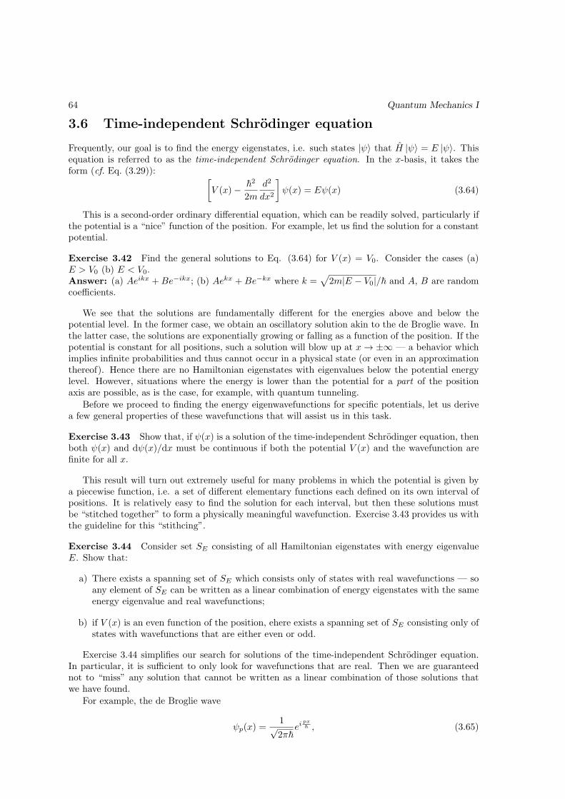
3.6 Time-independent Schrodinger equation

Frequently, our goal is to find the energy eigenstates, i.e. such states |ψ⟩ that H |ψ⟩ = E |ψ⟩. Thisequation is referred to as the time-independent Schrodinger equation. In the x-basis, it takes theform (cf. Eq. (3.29)): [

V (x)− ~2

2m

d2

dx2

]ψ(x) = Eψ(x) (3.64)

This is a second-order ordinary differential equation, which can be readily solved, particularly ifthe potential is a “nice” function of the position. For example, let us find the solution for a constantpotential.

Exercise 3.42 Find the general solutions to Eq. (3.64) for V (x) = V0. Consider the cases (a)E > V0 (b) E < V0.Answer: (a) Aeikx +Be−ikx; (b) Aekx +Be−kx where k =

√2m|E − V0|/~ and A, B are random

coefficients.

We see that the solutions are fundamentally different for the energies above and below thepotential level. In the former case, we obtain an oscillatory solution akin to the de Broglie wave. Inthe latter case, the solutions are exponentially growing or falling as a function of the position. If thepotential is constant for all positions, such a solution will blow up at x→ ±∞ — a behavior whichimplies infinite probabilities and thus cannot occur in a physical state (or even in an approximationthereof). Hence there are no Hamiltonian eigenstates with eigenvalues below the potential energylevel. However, situations where the energy is lower than the potential for a part of the positionaxis are possible, as is the case, for example, with quantum tunneling.

Before we proceed to finding the energy eigenwavefunctions for specific potentials, let us derivea few general properties of these wavefunctions that will assist us in this task.

Exercise 3.43 Show that, if ψ(x) is a solution of the time-independent Schrodinger equation, thenboth ψ(x) and dψ(x)/dx must be continuous if both the potential V (x) and the wavefunction arefinite for all x.

This result will turn out extremely useful for many problems in which the potential is given bya piecewise function, i.e. a set of different elementary functions each defined on its own interval ofpositions. It is relatively easy to find the solution for each interval, but then these solutions mustbe “stitched together” to form a physically meaningful wavefunction. Exercise 3.43 provides us withthe guideline for this “stithcing”.

Exercise 3.44 Consider set SE consisting of all Hamiltonian eigenstates with energy eigenvalueE. Show that:

a) There exists a spanning set of SE which consists only of states with real wavefunctions — soany element of SE can be written as a linear combination of energy eigenstates with the sameenergy eigenvalue and real wavefunctions;

b) if V (x) is an even function of the position, ehere exists a spanning set of SE consisting only ofstates with wavefunctions that are either even or odd.

Exercise 3.44 simplifies our search for solutions of the time-independent Schrodinger equation.In particular, it is sufficient to only look for wavefunctions that are real. Then we are guaranteednot to “miss” any solution that cannot be written as a linear combination of those solutions thatwe have found.

For example, the de Broglie wave

ψp(x) =1√2π~

eipx~ , (3.65)

3.7. BOUND STATES 65

associated with momentum eigenstate |p⟩, is a solution of the time-independent Schrodinger equationwith energy eigenvalue E = p2/2m. The same is true for the wavefunction

ψ−p(x) =1√2π~

e−ipx~ , (3.66)

which is the de Broglie wave for momentum eigenstate |−p⟩. But then the real wavefunctions

ψp,+(x) =ψp(x) + ψ−p(x)

2=

1√2π~

cospx

~(3.67)

and

ψp,−(x) =ψp(x)− ψ−p(x)

2i=

1√2π~

sinpx

~(3.68)

also represent energy eigenstates with the same eigenvalue. The de Broglie wavefunctions (3.65) and(3.66) — and hence can any other wavefunction corresponding to the same energy — can be writtenas linear combinations of these real wavefunctions.

3.7 Bound states

Bound states are characterized by a wavefunction that tends to zero at |x| → ±∞, so the particleexhibits some degree of localization. This property is typical for energy eigenstates in well-shapedpotentials, i.e. such fields in which the particle is attracted towards a certain location or a set oflocations. Physical examples include a pea inside a glass, a ball on a spring (harmonic oscillator)or an electron within an atom. For this type of potentials, we usually take advantage of Ex. 3.44(a)and look for solutions of the time-independent Schrodinger equation in the real domain.

Exercise 3.45 Consider a potential V (x) that approaches a particular value V0 at |x| → ±∞.Show that an energy eigenstate is bound if and only if its energy does not exceed V0.

As we shall see in the examples below, the boundary conditions imposed on the behavior of thewavefunction at |x| → ±∞ can be satisfied only for specific, discrete values of the energy. In otherwords, a well-shaped potential features a discrete or quantized spectrum of energy eigenvalues.

V0

?a / 2 a / 2

0

V0

Figure 3.3: Potential for Ex. 3.69

Exercise 3.46 Find the energy eigenvalues and eigenwavefunctions for the finite square well po-tential:

V (x) =

{V0 for |x| > a/2

0 for |x| ≤ a/2(3.69)

a) Write the general solution for each region where the potential is constant. Eliminate unphysicalterms that grow at infinity.

b) Apply the statement of Ex. 3.43 to “stitch” these results together. Derive the transcendentalequation defining the energy eigenvalues.


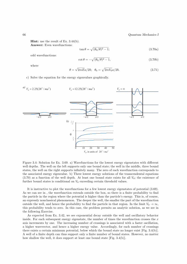
Hint: use the result of Ex. 3.44(b).Answer: Even wavefunctions:

tan θ =√

(θ0/θ)2 − 1; (3.70a)

odd wavefunctions:

cot θ = −√

(θ0/θ)2 − 1, (3.70b)

where

θ =√2mEa/2~; θ0 =

√2mV0a/2~. (3.71)

c) Solve the equation for the energy eigenvalues graphically.

0 10 20 30 40 50

-a/2 a/2

a)

b)

, in units of 2 22 / mah0V

q

-a/2 a/2 -a/2 a/2

2 2

0 12.25(2 / )V ma= h2 2

0 2.25(2 / )V ma= h 0V = ¥

Figure 3.4: Solution for Ex. 3.69. a) Wavefunctions for the lowest energy eigenstates with differentwell depths. The well on the left supports only one bound state; the well in the middle, three boundstates, the well on the right supports infinitely many. The zero of each wavefunction corresponds tothe associated energy eigenvalue. b) Three lowest energy solutions of the transcendental equations(3.70) as a function of the well depth. At least one bound state exists for all V0; the existence offurther bound states is conditional on V0 exceeding certain threshold values.

It is instructive to plot the wavefunctions for a few lowest energy eigenstates of potential (3.69).As we can see in , the wavefunction extends outside the box, so there is a finite probability to findthe particle in the region where the potential is higher than the particle’s energy. This is, of course,an expressly nonclassical phenomenon. The deeper the well, the smaller the part of the wavefunctionoutside the well, and hence the probability to find the particle in that region. In the limit V0 →∞,this probability tends to zero. In this case, the problem permits an analytic solution, as we see inthe following Exercise.

As expected from Ex. 3.42, we see exponential decay outside the well and oscillatory behaviorinside. For each subsequent energy eigenstate, the number of times the wavefunction crosses the xaxis increments by one. The increasing number of crossings is associated with a faster oscillation,a higher wavevector, and hence a higher energy value. Accordingly, for each number of crossingsthere exists a certain minimum potential, below which the bound state no longer exist [Fig. 3.4(b)].A well of a finite depth can thus support only a finite number of bound states. However, no matterhow shallow the well, it does support at least one bound state [Fig. 3.4(b)].

3.7. BOUND STATES 67

Exercise 3.47 Find the energy eigenvalues and bound stationary states for Ex. 3.46 in the caseV0 →∞ (the potential referred to as the potential box ).Answer: A discrete energy spectrum with

En =~2π2n2

2ma2; (3.72)

ψn(x) =

√

2a sin

(nπxa

), even n√

2a cos

(nπxa

), odd n.

, −a/2 ≤ x ≤ a/2; (3.73)

ψn(x) = 0, |x| > a/2.

These wavefunctions are displayed in Fig. 3.4(a), right panel.

The above wavefunctions exhibit a number of interesting features:

• ψ(x) = 0 outside the box;

• dψ(x)/dx exhibits discontinuities at x = ±a/2;

• ψ(x) is continuous for all position values.

In order to better understand them, let us rewrite the time-independent Schrodinger equation (3.64)as follows:

− ~2

2m

d2

dx2ψ(x) = [E − V (x)]ψ(x). (3.74)

Outside the box, V (x) =∞. Therefore, if ψ(x) is nonzero, the right-hand side of the above equationbecomes infinite, and so does d2ψ(x)/dx2 over a continuous interval of positions. This is not possiblefor any regular function.

The infinite value of the potential outside the box also implies that the conditions of Ex. 3.43 arenot fulfilled, so neither the wavefunction nor its derivative have to be continuous at x = ±a/2. In thepresent case, we observe that the wavefunction is continuous but the derivative is not. Intuitivelythis can be understood as follows. A discontinuity in dψ(x)/dx implies that the right-hand side ofEq. (3.74) is singular, i.e. it takes on infinite values — which is exactly what we have in our problem.But if the wavefunction itself is not continuous, the potential must exhibit singularity of the secondorder — i.e. be a derivative of a function that is already singular. Such potentials are extremelyexotic and do not occur within the scope of basic quantum mechanics. Therefore, in solving thetime-independent Schrodinger equation in the position basis, it is generally safe to assume that thewavefunction behaves continuously.

Exercise 3.48 For the eigenstates of the previous problem, find the uncertainties of the positionand momentum and verify the uncertainty principle.

Exercise 3.49 Consider the state ψ(x) ={Ax for |x|<a/20 for |x|≥a/2 (A = 2

√3/a3/2 being the norm) in the

potential of the previous problem. Find the energy spectrum of this state, i.e. the probabilitiespr(En) to measure each energy eigenvalue. Show that these probabilities sum up to 1. (Hint:∑

1/n2 = π2/6.)

Exercise 3.50 For the finite well potential (3.69):

a) Find analytically the approximate corrections to the first two energy levels of an infinitely deeppotential well (Ex. 3.47) when it is replaced by a finite well with a V0 ≫ E1, where E1 is givenby Eq. (3.72).

b) Find numerically all energy eigenvalues for k0a = 10. How many energy levels are therealtogether? Is your result for n = 1, 2 consistent with the result of part (a)?


c) What is the minimum depth that is required in order for the well to contain a given numberN of bound eigenstates?

Exercise 3.51 Find the transcendental equation for the energy eigenvalues associated with thebound stationary states of the potential

V (x) =

+∞ for x ≤ 0;0 for 0 < x ≤ a;V0 for x > a.

Compare your result with that of Ex. 3.69.

V0

a

?

0

0

Figure 3.5: Potential for Ex. 3.51

Exercise 3.52 Solve the time-independent Schrodinger equation for the finite well potential (3.69)anlytically in the limit of an infinitely deep and narrow potential well: a → 0, V0 = W0/a, withW0 = const. How many bound states can this well contain?

Exercise 3.53 Find the energy eigenvalues and the bound stationary states of the potential V (x) =−W0δ(x)

a) (a) using the position basis; (b) using the momentum basis.

Verify the consistency of your solutions with one another and with the result of Ex. finitewellEx2Hint: ∫ +∞

−∞

1

1 + x2dx = π;

∫ +∞

−∞

1

(1 + x2)2dx = π/2 (3.75)

Answer: Single eigenstate with E = −W 20m/2~2. Wavefunctions:

ψ(x) =√k0

{e−k0x at x > 0

ek0x at x ≤ 0;

ψ(k) =2k

3/20√

2π(k20 + k2),

where k0 =√−2mE/~ =W0m/~2.

Exercise 3.54 A particle is in the bound state of the potential V (x) = −W0δ(x). The potentialsuddenly changes to V (x) = −2W0δ(x). Find the probability that the particle will remain in abound state.

Exercise 3.55 Investigate the bound states of the potential V (x) = −W0δ(x− a)−W0δ(x+ a).

a) Find the transcendental equation for the energy eigenvalues (consider both the even and oddcase).

b) Show that in the limit a→∞ this equation becomes identical to that for a single well.

3.8. UNBOUND STATES 69

c) Find the first order correction to the solution of the transcendental equation for the case of abeing very large (k0a≫ 1), but not infinite.

Exercise 3.56 Under the conditions of the previous problem (distant wells), suppose the particleat the moment t = 0 is localized at the first well (i.e. its wavefunction is that of Ex. 3.53 centeredat x = a). What is the probability of finding it in the second well as a function of time?

Exercise 3.57∗(Kronig-Penney solid state model). Find allowed ranges (zones) of energy eigenvaluesfor a particle in a periodic potential field

a)

V (x) =

∞∑n=−∞

~2k0m

δ(x− na); (3.76)

b)

V (x) = −∞∑

n=−∞

~2k0m

δ(x− na). (3.77)

Consider both limiting cases k0a≫ 1 and k0a≪ 1.

Exercise 3.58∗ Show that bound energy eigenstates states of a pointlike particle with a single degreeof freedom cannot be degenerate.

3.8 Unbound states

Unbound wavefunctions take finite, nonzero values at infinity. In contrast to bound states, stationaryunbound states possess the following properties.

• Their energy exceeds the value of the potential at x→ −∞ or x→ +∞ or both.

• They are not normalizable.

• Their associated energy eigenvalues form a continuous spectrum.

• They can be degenerate: more than one linearly independent wavefunctions may correspondto a specific energy eigenvalue.

The most straightforward example of the unbound state is the momentum eigenstate |p⟩ in freespace. The associated energy eigenvalue, E = p2/2m, exceeds the potential V (x) = 0 at infinity.Since there exists a momentum eigenstate |p⟩, where p =

√2mE, for every energy value, these values

form a continuum. For every energy value, states |±p⟩ are degenerate.Let us now study the unbound energy eigenstates that correspond to more complicated potential

energy functions.

Exercise 3.59 (the single-step potential). Find the eigenstates of the Hamiltonian

V (x) =

{0 for x ≤ 0

V0 for x > 0(3.78)

(Fig. 3.6) corresponding to a given energy E > V0. Show that, for every value of E, there existtwo linearly independent solutions. Choose the solutions that correspond to the following physicalsituations: (1) a wave approaching the step only from the left and (2) a wave approaching only fromthe right.Answer (in the notation of Fig. 3.6). First solution (D = 0):

B = Ak0 − k1k0 + k1

; C = A2k0

k0 + k1, (3.79a)


Figure 3.6: Notation for the de Broglie component waves in a single-step potential (Ex. 3.59 and3.62)

and (2) an initial de Broglie wave approaching from the right (A = 0)

B = D2k1

k0 + k1; C = D

k1 − k0k0 + k1

. (3.79b)

Now let us try and relate our calculation to the intuitive physical picture of a material particleencountering a potential step. Making this connection may be difficult because the energy eigenstateis time independent, whereas the collision of a particle with a step, as we intuitively imagine it, isan intrinsically time-dependent phenomenon.

Some intuitive connection can be drawn in we recall that even stationary states experiencequantum evolution, which consists of the time-dependent phase factor e−iEt/~. Accordingly, thede Broglie waves associated with amplitudes A and C (we will call them the A- and C-waves,respectively) move to the right while the B-wave is moving to the left.

This situation resembles a continuous laser beam which propagates from air into glass, experi-encing partial reflection in accordance with the Fresnel equations. Similarly to the situation withthe quantum particle, the reflection is not an instantaneous event but a stationary process whichcomprises motion of the electromagnetic waves in space and time. In fact, if we compare the Fresnelequations for the field amplitudes with Eqs. (3.79), and take into account that the optical wavevec-tor is proportional to the index of refraction, we will find these two sets of equations completelyidentical!

An interesting feature of the result (3.79) is that the amplitude C of the transmitted de Brogliewave is higher than the amplitude A of the incident one. The particle appears more likely to befound behind the step than within the same interval in front of it. Doesn’t that contradict the lawof conservation of matter?

We can gain some insight for answering this question by looking at optical waves again. Accordingto Fresnel equations, the amplitude of the light wave inside glass is also higher than that in the air.However, this does not conflict with the law of energy conservation because the wave inside the glasstravels at a lower speed. Accordingly, the flux of energy (Poynting vector) carried by the transmittedwave is lower than that of the incident wave.

A similar argument can be drawn in the case of a quantum particle. It is not the probabilitydensity associated with the wavefunction that determines the conservation of matter but rather theprobability density current studied in Sec. 3.5. As we learned in Ex. 3.38, this current is proportionalnot only to the squared absolute value of the de Broglie wave amplitude, but also to its momentum.If we take this into account, we will observe that the conservation of matter is perfectly sustained.

Exercise 3.60 Find the probability density currents for each wave in Eqs. (3.79a) and (3.79b).Find the reflection and transmission coefficients for these currents and show that their sum is one.What is the behavior of these coefficients for E → V0 and E →∞?

Exercise 3.61 Solve Ex. 3.59 for energies below V0. Verify that the reflection coefficient is one.

3.8. UNBOUND STATES 71

An even better overview of the quantum reflection of a particle on a potential step can be obtainedif we combine multiple de Broglie waves into a Gaussian wavepacket and then study its evolution ina way that is similar to Ex. 3.31, but in the potential given by Eq. (3.78).

Exercise 3.62 Find the evolution of a Gaussian packet initially described by Eq. (3.38) with apositive p0 and negative a in the single-step potential field (Fig. 3.6). Assume that

• |a| ≫ d so the wavepacket is at first entirely to the left of the step;

• d2 ≫ ~t/m so spreading of the wavepacket (Ex. 3.31) can be neglected;

• the initial average energy of the particle E = p20/2m is greater than V0;

• the rms momentum uncertainty of the wavepacket ~/2d is small compared to the averagemomentum ~k1 =

√2m(E0 − V0) behind the step.

As we see, upon encountering the step the initial wavepacket splits. A part of the wavepacketcontinues to propagate past the step with a lower group velocity, and another part reflects off thestep and begins to propagate in the backward direction.

As the final comment about the potential step problem let us note that the fact that the particlehas a probability to bounce off a potential step that is lower than the particle’s energy or evennegative (as in the case described by Eq. (3.79b)) is expressly quantum. Any classical particlewill simply “fly above” the potential step, reducing or increasing the speed but never reversing thedirection of its motion.

Even more nonclassical is the effect of quantum tunneling, which we study next.

Figure 3.7: Tunnelling through a barrier (Ex. 3.63)

Exercise 3.63 Consider the potential in Fig. 3.7, i.e.

V (x) =

{0 for x ≤ 0 or x > L

V0 for 0 < x ≤ L(3.80)

a) What is the degeneracy of energy levels?

b) Find the solution of the time-independent Schrodinger equation corresponding to a de Brogliewave entering from the left and 0 < E < V0.

c) Find the transmission and reflection coefficients for the probability current. Is their sum equalto one?

d) Investigate the boundary cases E → 0 and E → V0.

Answer.

T =

∣∣∣∣EA∣∣∣∣2 =

4k20k21

4k20k21 + (k21 + k20)

2 sinh(k1L); (3.81a)

R =

∣∣∣∣BA∣∣∣∣2 =

(k21 + k20)2 sinh(k1L)

4k20k21 + (k21 + k20)

2 sinh(k1L). (3.81b)


We observe that a particle encountering a finite potential barrier which is higher than the parti-cle’s kinetic energy has a finite probability of “tunnelling” through this barrier. This phenomenonhas, of course, no analogy in classical physics.

Exercise 3.64 Repeat Ex. 3.63 for E > V0. Is the sum of the reflection and transmission coeffi-cients equal to one in this case?

Exercise 3.65 Calculate the reflection and transmission for scattering on a delta-potential V (x) =W0δ(x). Compare your results with those obtained from Eqs. (3.81) for an infinitely thin and highrectangular potential barrier (L→ 0, V0 =W0/L).

Exercise 3.66∗ Perform numerical investigations of the propagation of a Gaussian wavepacket in apotential shown in Fig. 3.7. Make simplifying assumptions as necessary. What time does it take thewavepacket to penetrate the barrier?

Solving the previous exercise, we find that the wavepacket spends no time inside the barrier.The tunnelling occurs instantaneously : the transmitted wavepacket emerges behind the barriersimultaneously with the initial wavepacket being absorbed. This can be traced back to the fact thatthe C- and D-waves have a constant phase, so the complex argument Argψ(x) of the wavefunctionat points x = 0 and x = L is the same. Schrodinger evolution of a de Broglie wave is equivalent to aphase shift, and the lack thereof translates into a zero delay between the incident and transmittedwaves, resulting in an infinite group velocity.

In Chapter 2 we already encountered a quantum phenomenon that appeared to enable faster-than-light communication, but, after careful analysis, found this to be only an illusion. The samecan be said about the present situation, although the reason is different. Let us ask ourselves: atwhat moment does an observer behind the barrier learn that the particle is entering the barrier? Isit when a half of the wavepacket has emerged from the barrier, three-fourths or nine-tenths?

The correct answer is, much earlier than that. From complex analysis, we know that the Gaussianfunction is analytic: any fragment of this function allows one to reconstruct its behavior in the entirecomplex plane. Therefore, any observer anywhere in space is aware of the presence of the particlewith a Gaussian wavefunction, and can predict its evolution, from the initial moment of our analysis.With this in mind, it makes no sense to talk about instant communication.

What if we instead tried a different wavefunction, for example, of the top-hat shape (3.9), whichtakes on nonzero values only within a finite spatial region? The problem with such wavefunctionsis that, in contrast to the Gaussian case, their decompositions into the momentum basis are notnarrow: for example, the Fourier transform of the top-hat function is the sinc function. For suchfunctions, we cannot apply the approximations used to calculate the evolution of Gaussian functions(see Ex. 3.62) — for example, because they have significant components corresponding to energiesabove the barrier. This tremendously complicates the calculations; however, if the analysis is performthoroughly, it will exclude any possibility of superluminal propagation.

3.9 Harmonic oscillator

3.9.1 Annihilation and creation operators

The harmonic oscillator is a physical system of primary importance. Its applications extend farbeyond the motion of simple mechanical systems. For example, the quantum description of light,not limited by the single-photon subspace studied in Chapters 1 and 2, is identical to that of theharmonic oscillator. Other applications include solid state physics, molecular spectroscopy and evenatomic physics.

Figure 3.8(a) displays a classical harmonic oscillator — a “ball on a spring”. The oscillationfrequency ω is related to the spring constant k in accordance with k = mω2. Because the potentialenergy of the spring is U = kx2/2, its full Hamiltonian is given by

H =p2

2m+mω2x2

2(3.82)

3.9. HARMONIC OSCILLATOR 73

x

p

max maxp m xw=

maxx

k m

a) b)

x

Figure 3.8: A classical harmonic oscillator. a) The physical model; b) motion in the phase space.

The trajectory is elliptical with the half-axes pmax = mωxmax.The harmonic oscillator is a typical potential well. Therefore its energy eigenstates are bound and

nondegenerate (see Ex. 3.58). It is possible to find the wavefunctions of these states by solving thetime-independent Schrodinger equation (3.64) in the position basis. However, because the harmonicoscillator is such an important physical system, we choose to develop its quantum theory in a moregeneral fashion. We begin by rescaling the position and momentum observables so they are moreconvenient to operate with.

Exercise 3.67 Rescale the position and momentum observables, i.e. define new observables (X =Ax,P = Bp) with proportionality constants A and B such that (a) in the new variables (X, P ) thephase space trajectory is circular [Pmax = Xmax, see Fig. 3.8(b)] and (b) for corresponding quantumoperators, [X, P ] = i.Answer:

X = x

√mω

~; P =

p√mω~

(3.83)

Exercise 3.68 Show that the rescaled observables X and P are dimensionless.

Exercise 3.69 If a certain quantum state has wavefunctions ψ(x) = ⟨x| ψ⟩ and ψ(p) = ⟨p| ψ⟩, whatare the corresponding wavefunctions ψ(X) = ⟨X| ψ⟩ and ψ(P ) = ⟨P | ψ⟩ in the rescaled variables?Write the relations analogous to (3.33) for converting wavefunctions between X- and P - bases.


⟨X| P |ψ⟩ = −i ddX

ψ(X); ⟨P | X |ψ⟩ = id

dPψ(P ). (3.84)

Exercise 3.71 Write the Hamiltonian in terms of X and PAnswer:

H =1

2~ω(X2 + P 2

). (3.85)

We now proceed to defining and studying the properties of the two operators which, as we shallsee in the next subscection, enact transitions between adjacent energy eigenstates.

Definition 3.2 The annihilation operator is defined as follows:

a =1√2

(X + iP

); (3.86)

The operator a† is called the creation operator.

Exercise 3.72 Show that:


a) the creation operator is

a† =1√2

(X − iP

); (3.87)

b) the creation and annihilation operators are not Hermitian;

c) their commutator is

[a, a†] = 1; (3.88)

d) position and momentum can be expressed as

X =1√2

(a+ a†

); P =

1

i√2

(a− a†

); (3.89)

e) the hamiltonian can be written as

H = ~ω(a†a+

1

2

); (3.90)

f) the commutators

[a, a†a] = a; [a†, a†a] = −a†. (3.91)

3.9.2 Fock states

Our next goal is to find eigenvalues and eigenstates of the Hamiltonian. Because of Eq. (3.90), theyare also eigenstates of operator n = a†a.

Exercise 3.73 Suppose some state |n⟩ is an eigenstate of the operator a†a with eigenvalue n:

a†a |n⟩ = n |n⟩ (3.92)

Show that

a) the state a |n⟩ is also an eigenstate of a†a with eigenvalue n− 1;

b) the state a† |n⟩ is also an eigenstate of a†a with eigenvalue n+ 1.

Hint: Use Eq. (3.91).

As we know, energy spectra of bound states are nondegenerate, i.e. for each value of n thereexists no more than a single energy eigenstate |n⟩. Therefore Ex. 3.73 shows that the states a |n⟩and a† |n⟩ are proportional to states |n− 1⟩ and |n+ 1⟩, respectively. The proportionality coefficientcan be found from the requirement that the energy eigenstates must be normalized.


a)

a |n⟩ =√n |n− 1⟩ ; (3.93a)

b)

a† |n⟩ =√n+ 1 |n+ 1⟩ ; (3.93b)

Hint: use ⟨n| a†a |n⟩ = n.


We found that, if state |n⟩ with energy ~ω(n+1/2) exists as a physical state (i.e. is a normalizedelement of the Hilbert space), so does the state |n− 1⟩ with energy ~ω(n − 1/2). Similarly, states|n− 2⟩, |n− 3⟩, and so on must also exist. Continuing this chain for sufficiently many steps, we willend up with energy eigenstates with negative energy values.

How can we resolve this contradiction? The only way is to assume that n must be nonnegativeinteger so the chain is broken at n = 0, in which case

a |0⟩ = |zero⟩ . (3.94)

Then (provided that the state |n = 0⟩ exists), energy eigenstates form an infinite set with equidistanteigenvalues ~ω(n+ 1/2).

Definition 3.3 Energy eigenstates of a harmonic oscillator are called Fock or number states. Thestate |0⟩ is called the vacuum state.

Exercise 3.75 Express |n⟩ through |0⟩.Answer:

|n⟩ =(a†)n

√n!|0⟩ (3.95)

Exercise 3.76 Calculate the wavefunction of the vacuum state in the position and momentumrepresentations.Hint: use Eqs. (3.84), (3.86) and (3.94).Answer:

ψ0(X) =1

π1/4e−X

2/2; ψ0(P ) =1

π1/4e−P

2/2. (3.96)

Note that the above wavefunctions are unique up to an arbitrary overall phase factor. For thevacuum state, by convention, we choose this factor so as to obtain a real and positive definitewavefunction in the position basis. It then automatically follows that the wavefunction in themomentum basis is also real and positive. Furthermore, as we shall see below, this conventionensures that the wavefunctions of all other Fock states are also real.

By having explicitly found the wavefunction of the vacuum states, we have proven its existence,and thus, automatically, the existence of all other Fock states — because these states are obtainedfrom the vacuum state by applying the creation operator.

Now the physical meaning of the eigenvalue n of operator n becomes also clear: this is thenumber of excitation quanta in the harmonic oscillator. The number of such quanta is alwaysinteger and, because energy levels are equidistant, all of them have the same energy, ~ω. In thisway, the excitation quanta in a harmonic oscillator resemble particles and, in many cases, they dobehave like particles. Among the examples are photons in an optical pulse phonons in a vibrationalmode of a solid state.

Exercise 3.77 a) By applying Eq. (3.95), calculate the wavefunctions of Fock states |1⟩ and|2⟩.

b) Show that the wavefunction of an arbitrary Fock state |n⟩ is given by

ψn(X) =Hn(X)

π1/4√2nn!

e−X2/2, (3.97)

where Hn(X) are the Hermite polynomials,

Hn(X) = (−1)nex2/2 dn

dXne−x

2/2. (3.98)

As we have proven in Ex. 1.76, eigenstates of a Hermitian operator form a basis of the relevantHilbert space. Since the proof was made for Hilbert spaces of finite dimensions, one should generallybe careful applying that result to infinite-dimensional spaces, such as those studied in this chapter.For example, all the eigenstates of the infinite potential box (Ex. 3.47) have wavefunctions that


n = 0

n = 1

n = 2

n = 3

X0

Figure 3.9: Wavefunctions of the first three energy levels of a harmonic oscillator.

vanish outside the box, so they do not span the space of all possible wavefunctions. On the otherhand, these wavefunctions do span the space of all quantum states that are localized within thebox, i.e. are physically allowed under this potential. Even more complicated is the situation with afinite well (Ex. 3.69), whose energy eigenstates combine a discrete (for E < V0) and continuous (forE ≥ V0) spectra.

The situation with the Harmonic oscillator is convenient in this respect because, on the onehand, there are no quantum states that are not physically allowed and, on the other hand, the entireenergy spectrum is discrete. As a result, the Fock states do form an orthonormal basis in the Hilbertspace. This statement also follows from mathematical properties of the Hermite functions (3.97),which are known to form a basis in the Hilbert space of all normalizable functions defined on thereal axis.

It is instructive to compare the wavefunctions of the Fock states with those of energy eigenstatesof the finite potential well (shown in Fig. 3.4). In both cases, the wavefunctions exhibit oscillatorybehavior inside the well and exponentially fall off outside. The difference is that the energy levelsare equidistant for the harmonic oscillator, but not equidistant for the rectangular well. Also, eacheigenwavefunction of the well is defined in a piecewise fashion [see Eqs. (8.19) and (8.28)] while forthe harmonic oscillator potential it is a single elementary function.

Exercise 3.78 For an arbitrary |n⟩, calculate ⟨X⟩, ⟨∆X2⟩, ⟨P ⟩, ⟨∆P 2⟩ and verify the uncertaintyprinciple.Hint: Rather than integrating the wavefunctions, it is more convenient to employ Eqs. (3.89) and(3.93).

Note 3.2 The vacuum state is the only minimum-uncertainty Fock state.

Exercise 3.79 Find the evolution of the state α |0⟩+ β |1⟩; calculate the time dependence of ⟨X⟩,⟨P ⟩ and plot the trajectory in the phase space.Answer (for real α, β):

⟨X⟩ =√2αβ(cosωt); ⟨P ⟩ = −

√2αβ(sinωt).

This last result is remarkable. The Fock states themselves are stationary and thus exhibit notime variation of the mean position and momentum. But in their linear combinations, the meanposition and momentum oscillate similarly to those of a classical harmonic oscillator. Of course,this behavior is still very dissimilar to classical: the mean values of the position and momentum aremicroscopic, and their scale is compatible to that of their own uncertainties. In the next subsectionwe will study those states whose behavior under Schrodinger evolution resembles classical muchmore significantly.

3.9.3 Coherent states

The coherent state is the closest quantum approximation of the classical picture of the harmonicoscillator motion. As we shall see, in this state the mean position and momentum vary as functions of


time in the same way as do those of a classical ball on a spring. The amplitude of this oscillation canbe arbitrarily high, but the position and momentum uncertainties remain as low as in the vacuumstate. Because of their classical-like behavior, coherent states frequently occur in nature, not onlyin mechanical oscillators, but also in other “incarnations” of the harmonic oscillator. For example,the quantum state of light in a laser pulse is also a coherent state.

Definition 3.4 The coherent state |α⟩ is an eigenstate of the annihilation operator with eigenvalueα:

a |α⟩ = α |α⟩ . (3.99)

The quantity |α| is called the amplitude, Argα the phase of the coherent state.

Exercise 3.80 For a coherent state |α⟩, show that its wavefunctions in the position and momentumbases are given by

ψα(X) =1

π1/4e−i

PαXα2 eiPαXe−

(X−Xα)2

2 ; (3.100)

ψα(P ) =1

π1/4ei

PαXα2 e−iXαP e−

(P−Pα)2

2 , (3.101)

where

Xα =√2Reα; Pα =

√2Imα. (3.102)

The overall phase factors e±iPαXα/2 are included into Eqs. (3.100) and Eq. (3.101) as a matterof convention in order to make these two equations (which are obtained from one another by meansof a direct or inverse Fourier transform) look similar. We will see shortly that this convention is infact pretty useful.

By comparing Eq. (3.100) with Eq. (3.38) we observe that the coherent state wavefunction is aGaussian wavepacket centered at

√2Reα. Aside from a linearly varying phase factor and the shift

of the center, the shape of the wavefunction is identical to that of the vacuum state. This is notsurprising given that, according to the above definition, the vacuum state is a coherent state withzero amplitude. In fact, one can show the following:

Exercise 3.81 Show that the coherent state can be obtained from the vacuum state by applyingdisplacement operators

|α⟩ = e−iPαXα/2eiPαXe−iXαP |0⟩ (3.103)

= eiPαXα/2e−iXαP eiPαX |0⟩ .

Exercise 3.82 Show that the expectation values of the position and momentum in coherent state|α⟩ are

⟨X⟩ =√2Reα; ⟨P ⟩ =

√2Imα. (3.104)

Show that the uncertainties of these observables equal⟨∆X2

⟩=⟨∆P 2

⟩=

1

2. (3.105)

One can picture the coherent state in the phase space as a circle positioned at points (√2Reα,

√2 Imα)

(Fig. 3.10). The radius of the circle, 1/√2, symbolically represents the standard deviation of the

position and momentum, which are independent of the coherent amplitude9. In all coherent states,similarly to the vacuum state, the position-momentum uncertainty product takes the minimumpossible value.

Now let us find the Schrodinger evolution of the coherent state in time. To this end, we decomposethe coherent state into energy eigenstates and apply the evolution operator to each of these states.

9In fact, this circle has more than just a symbolic value. The behavior of uncertainties in the phase space isdescribed by the so-called Wigner function, which is the analog of the classical phase-space probability density.


Arg a

2 Rea

2 Ima

X

P

Figure 3.10: The phase space picture and evolution of the position and momentum observables inthe coherent state.

Exercise 3.83∗ Show that the coherent state can be written as

|α⟩ = e−|α|2/2eαa†e−α

∗a |0⟩ . (3.106)

Show that Eq. (3.106) can be simplified as follows:

|α⟩ = e−|α|2/2eαa†|0⟩ . (3.107)

Hint: use Eq. (3.103) and the Baker-Hausdorff-Campbell formula (1.70).

Exercise 3.84 Find the decomposition of the coherent state into the number basis (make sureyour answer is properly normalized).Answer:

|α⟩ = e−|α|2/2∑n

αn√n!|n⟩ . (3.108)

Now the role of the convention for the overall phase in Eqs. (3.100) and (3.100) becomes clear.With this convention, the decomposition (3.108) of the coherent state in to the Fock basis takes anextremely simple form.

If one performs an energy measurement on a coherent state, one will find, in accordance withEq. (3.108), that that the probability to project onto a particular Fock state is given by:

prn = |⟨n| α⟩|2 = e−|α|2 |α|2n

n!. (3.109)

This probability distribution is very well known in mathematical statistics. It is the so-called Poissondistribution, which expresses the probability of a number of events to occur within a given periodof time if these events occur with a known average rate and independently of each other. Let usdistract ourselves from pure quantum physics for a few minutes and study the properties of thisdistribution.

Exercise 3.85 Find ⟨n⟩, ⟨∆n2⟩ for a coherent state.Answer: ⟨n⟩ = ⟨∆n2⟩ = |α|2.

For example, in a certain city, 25 babies are born per day on average. The exact number ofbabies that are born on each day varies: sometimes there are exactly 25, sometimes (for example)


22, and sometimes 32. The probability that a specific number n of babies are born on some specificday is then given by Eq. (3.109) with ⟨n⟩ = |α|2 = 25. The mean square uncertainty in the numberof babies equals

√⟨∆n2⟩ =

√⟨n⟩ = 5, i.e. on a typical day it is much more likely to see 20 or 30

babies rather than 10 or 40 (Fig. 3.11).

10 20 30 40

0.05

0.10

0.15

n

prn

Figure 3.11: the Poisson distribution with ⟨n⟩ = 4 (empty circles) and ⟨n⟩ = 25 (filled circles).

Although the absolute uncertainty of n increases with ⟨n⟩, the relative uncertainty√⟨∆n2⟩/ ⟨n⟩

decreases. In our example above, the relative uncertainty is 5/25 = 20%. But in a smaller town,where ⟨n⟩ = 4, the relative uncertainty is as high as 2/4 = 50%.

Returning to the quantum oscillator, the higher the amplitude of the coherent state, the loweris the relative uncertainty in the number of excitation quanta within that state. For example, if wemeasure the energies of laser pulses (which are in the coherent state), the observed value will varyfrom pulse to pulse — the phenomenon known as the shot noise. For a higher intensity laser beam,with a higher average pulse energy, the relative magnitude of the shot noise will decrease. The moremacroscopic the coherent state becomes, the less significant are its quantum features.

Exercise 3.86 A laser of wavelength λ = 800 nm emits pulses with a repetition rate f = 100MHz. The average power of the laser is P = 1 Watt. Calculate

a) the mean energy of each laser pulse;

b) the mean number of photons in each pulse;

c) the relative uncertainty in the energy of the pulses due to the shot noise.

How will the answer in part (c) change if the average laser power is P ′ = 1 µW?

Exercise 3.87 Show that ⟨α| α′⟩ = e−|α|2/2−|α′|2/2+α′∗α.

In regards to the last exercise, one may ask how come the coherent states associated with dif-ferent α’s are not orthogonal. Didn’t we prove in Ex. 1.76 that eigenstates of an operator form anorthonormal basis? The answer is that the statement of Ex. 1.76 only applies to Hermitian operator— and the annihilation operator is not Hermitian. Coherent states do form a spanning set, but theyare not orthogonal.

Exercise 3.88 Do eigenstates of the creation operator exist and if so, what is their decompositioninto the number basis?

Exercise 3.89 Show that the action of the evolution operator exp(iHt/~) upon the state α isgiven by

exp(−iHt/~) |α⟩ = e−iωt/2∣∣e−iωtα⟩ . (3.110)


This result is remarkable. Neglecting the overall quantum phase factor e−iωt/2, a coherentstate evolves into another coherent state with the same amplitude, but different phase. Note thedistinction between the quantum phase factor outside the ket in Eq. (3.110) (which does not reflectin any measurement results) and the coherent phase factor e−iωt inside the ket, which indicates adifferent eigenvalue of the annihilation operator and hence a physically different quantum state.

The role of the coherent phase is evident from Fig. 3.10. The Hamiltonian evolution of thecoherent state entails linear growth of the phase and hence the circular motion of the expectationvalues in the phase space. Assuming α real, we find:

⟨X⟩ =√2Re(e−iωtα) =

√2α cosωt;

⟨P ⟩ =√2Im(e−iωtα) =

√2α sinωt. (3.111)

Aside from a microscopic uncertainty, the behavior of the position and momentum observables inthe coherent state is identical to classical.

Exercise 3.90 Are coherent states stationary?

chapter three

Documents

position x

associated eigenstate

real value of x

momentum observable

momentum p

position eigenstatex

particles position

set of eigenstates