chapter ten general equilibrium and economic welfare
Post on 19-Dec-2015
221 views
TRANSCRIPT

Chapter Ten
General Equilibrium and Economic Welfare

© 2007 Pearson Addison-Wesley. All rights reserved. 10–2
焦點新聞
• 政院稅改方案 大幅調降營所稅綜所稅• 鋼價狂漲 暫不限制出口
–由於國內外鋼價急驟上揚,近期陸續有營造等相關業界建議政府希望限制廢鋼、鋼筋等出口。經濟部工業局表示,按照 WTO精神,禁止出口有可能損及台灣形象,同時也會打亂台灣既有鋼鐵產銷體系,造成業界的反彈,甚至危及單軋廠的生存,因此,是否禁止出口尚未定論。

© 2007 Pearson Addison-Wesley. All rights reserved. 10–3
General Equilibrium and Economic Welfare
• In this chapter, we examine five main topics– General equilibrium– Trading between two people– Competitive exchange – Production and trading– Efficiency and equity

© 2007 Pearson Addison-Wesley. All rights reserved. 10–4
General Equilibrium
• partial-equilibrium analysis– an examination of equilibrium and changes
in equilibrium in one market in isolation
• general-equilibrium analysis– the study of how equilibrium is determined
in all markets simultaneously

© 2007 Pearson Addison-Wesley. All rights reserved. 10–5
Feedback Between Competitive Markets
• Sequence of Events– We can demonstrate the effect of a shock
in one market on both markets by tracing the sequence of events in the two markets.
– Whether these steps occur nearly instantaneously or take some times depends on how quickly consumers and producers react.

© 2007 Pearson Addison-Wesley. All rights reserved.
Figure 10.1 Relationship Between the Corn and Soybean Markets Corn, Billion bushels per year
e0c
e1c
e3c
D0c
D1c
S3c
S0c
$2.15
$1.9171$1.9057
8.448.26138.227
(a) Corn Market
Soybeans, Billion bushels per year
e0s
e2s
e4s
D4s
D2s
S4s
S2s
S0s
D0s
$4.12
$3.8325$3.8180
2.072.05142.0505
(b) Soybean Market

© 2007 Pearson Addison-Wesley. All rights reserved. 10–7
Minimum Wages With Incomplete Coverage
• Minimum Wages With Incomplete Coverage– In the absence of a minimum wage, the
equilibrium wage is . – Applying a minimum wage, , to only one
sector causes the quantity of labor services demanded in the covered sector to fall.
– The extra labor moves to the uncovered sector, driving the wage there down to .
1w
2w
w

© 2007 Pearson Addison-Wesley. All rights reserved. 10–8
Figure 10.2 Minimum Wage with Incomplete Coverage
(b) Uncovered Sector
w1
w2
Lu2Lu
1
Du
Su
Lu, Annual hours
(a) Covered Sector
w1
w–
Lc2 Lc
1
Dc
Lc, Annual hours L, Annual hours
(c) Total Labor Market
w1
S
Lc1 Lu
1L1 = +
D

© 2007 Pearson Addison-Wesley. All rights reserved. 10–9
Trading Between Two People
• Endowments– an initial allocation of goods
• Pareto efficient– describing an allocation of goods or
services such that any reallocation harms at least one person

© 2007 Pearson Addison-Wesley. All rights reserved. 10–10
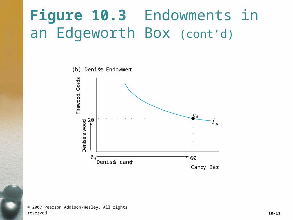
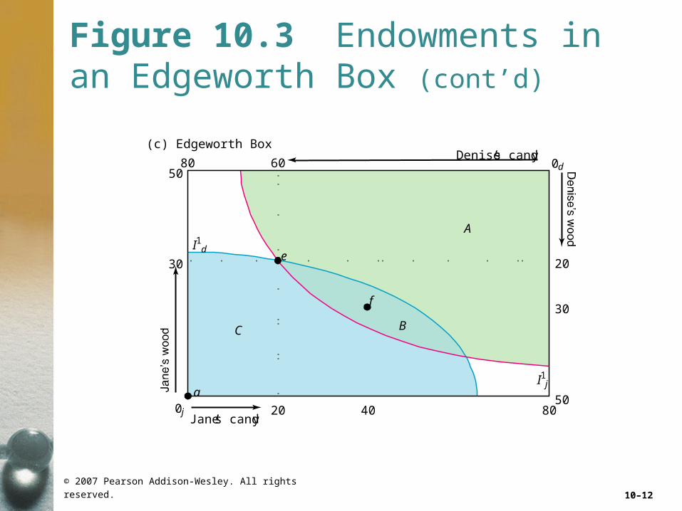
Figure 10.3 Endowments in an Edgeworth Box
I1j
(a) Jane’s Endowment
Jane’s candy20
30
Candy, Bars
0j
ej
© 2007 Pearson Addison-Wesley. All rights reserved. 10–11
Figure 10.3 Endowments in an Edgeworth Box (cont’d)
I1d
(b) Denise’s Endowment
Denise’s candy60
20
Candy, Bars
0d
ed
© 2007 Pearson Addison-Wesley. All rights reserved. 10–12
Figure 10.3 Endowments in an Edgeworth Box (cont’d)
(c) Edgeworth Box
Jane’s candy
Denise’s candy
C
A
B
20 40
608050
30e
a
f
8050
30
20
0j
0d
I1j
I1d

© 2007 Pearson Addison-Wesley. All rights reserved. 10–13
Mutually Beneficial Trades
• We make four assumptions about their tastes and behavior:– Utility maximization– Usual-shaped indifference curves– Nonsatiation– No interdependence

© 2007 Pearson Addison-Wesley. All rights reserved. 10–14
Figure 10.4 Contract Curve
Jane’s candy
Denise’s candy
20 40
608050
30
20
40g
c
d
e
b
a
fB
8050
30
20
Contract curve
0j
0d
I1jI2j
I3j
I4j
I 0d
I1dI2d
I3d
© 2007 Pearson Addison-Wesley. All rights reserved. 10–15
Mutually Beneficial Trades
• Trades are possible where indifference curves intersect because marginal rates of substitution are unequal.

© 2007 Pearson Addison-Wesley. All rights reserved. 10–16
Mutually Beneficial Trades
• To summarize, we can make four equivalent statements about allocation :1.The indifference curves of the two parties
are tangent at .2.The parties’ marginal rates of substitution
are equal at .3.No further mutually beneficial trades are
possible at .4.The allocation at is Pareto efficient: One
party cannot be made better off without harming the other.
f
f
f
ff

© 2007 Pearson Addison-Wesley. All rights reserved. 10–17
Mutually Beneficial Trades
• Indifference curves are also tangent at Bundles , , and , so these allocations, like , are Pareto efficient.
• By connecting all such bundles, we draw the contract curve: the set of all Pareto-efficient bundles.
bf
c d

© 2007 Pearson Addison-Wesley. All rights reserved. 10–18
Bargaining Ability
• All the allocations in area B are beneficial.
• Where will they end up on the contract curve between and ?
• That depends on who is better at bargaining.
b c
© 2007 Pearson Addison-Wesley. All rights reserved. 10–19
Competitive Exchange
• The First Theorem of Welfare Economics
– The competitive equilibrium is efficient: Competition results in a Pareto-efficient allocation—no one can be made better off without making someone worse off—in all markets.

© 2007 Pearson Addison-Wesley. All rights reserved. 10–20
Competitive Exchange
• The Second Theorem of Welfare Economics
– Any efficient allocations can be achieved by competition: All possible efficient allocations can be obtained by competitive exchange, given an appropriate initial allocation of goods.

© 2007 Pearson Addison-Wesley. All rights reserved. 10–21
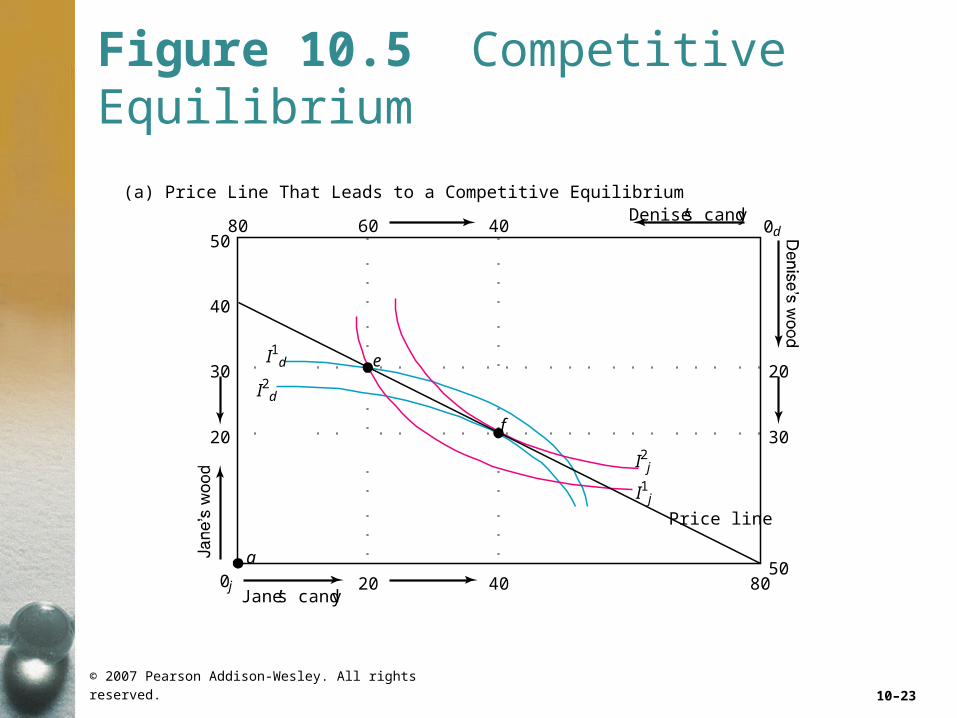
Competitive Equilibrium
• The initial endowment is .
a) If, along the price line facing Jane and Denise, and , they trade to point , where Jane’s indifference curve, , is tangent to the price line and to Denise’s indifference curve, .
$2wp $1cp
2jI
2dI
f
e
© 2007 Pearson Addison-Wesley. All rights reserved. 10–22
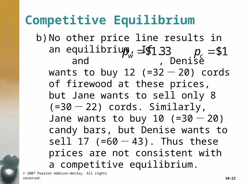
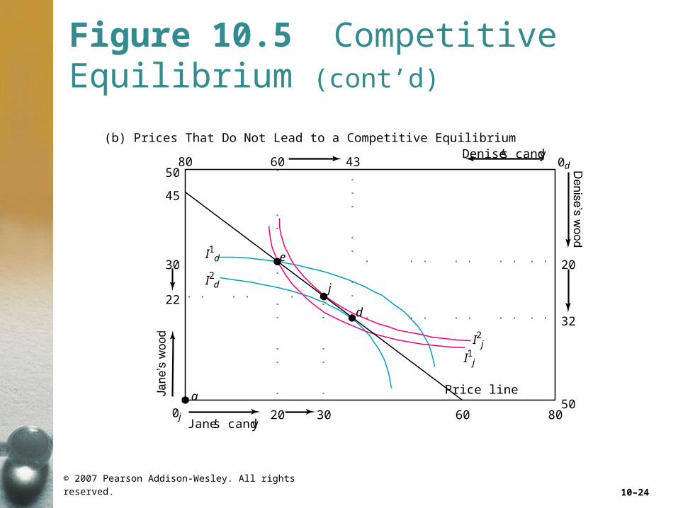
Competitive Equilibrium
b) No other price line results in an equilibrium, If and , Denise wants to buy 12 (=32 - 20) cords of firewood at these prices, but Jane wants to sell only 8 (=30 - 22) cords. Similarly, Jane wants to buy 10 (=30 - 20) candy bars, but Denise wants to sell 17 (=60 - 43). Thus these prices are not consistent with a competitive equilibrium.
$1.33wp $1cp
© 2007 Pearson Addison-Wesley. All rights reserved. 10–23
(a) Price Line That Leads to a Competitive Equilibrium
Jane’s candy
Denise’s candy
Price line
20 40
608050
30
40
20
40
e
a
f
8050
30
20
0j
0d
I1j
I2j
I1d
I2d
Figure 10.5 Competitive Equilibrium
© 2007 Pearson Addison-Wesley. All rights reserved. 10–24
Figure 10.5 Competitive Equilibrium (cont’d)
80
(b) Prices That Do Not Lead to a Competitive Equilibrium
Jane’s candy
Denise’s candy
Price line
20 30
608050
30
45
22
43
e
a
j
d
6050
32
20
0j
0d
I1j
I2j
I1d
I2d
© 2007 Pearson Addison-Wesley. All rights reserved. 10–25
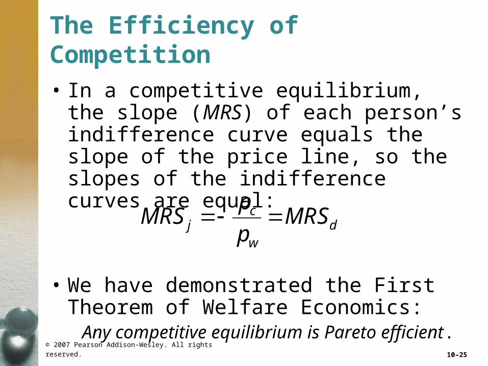
The Efficiency of Competition
• In a competitive equilibrium, the slope (MRS) of each person’s indifference curve equals the slope of the price line, so the slopes of the indifference curves are equal:
• We have demonstrated the First Theorem of Welfare Economics:
Any competitive equilibrium is Pareto efficient.
cj d
w
pMRS MRS
p
© 2007 Pearson Addison-Wesley. All rights reserved. 10–26
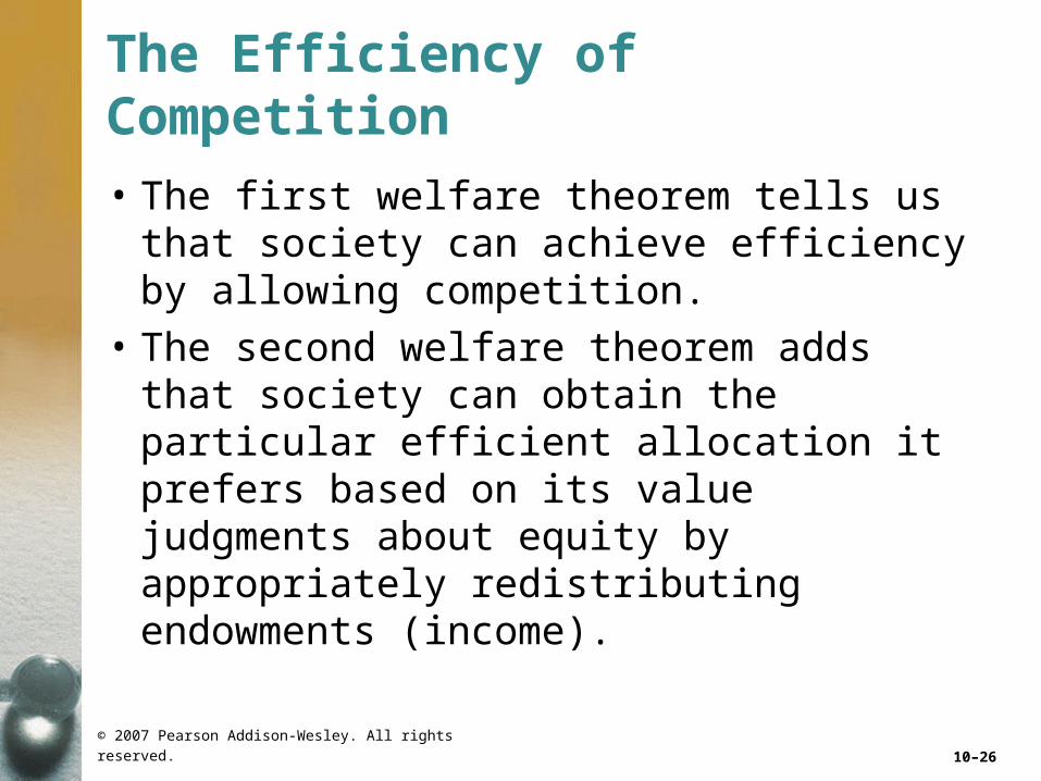
The Efficiency of Competition
• The first welfare theorem tells us that society can achieve efficiency by allowing competition.
• The second welfare theorem adds that society can obtain the particular efficient allocation it prefers based on its value judgments about equity by appropriately redistributing endowments (income).

© 2007 Pearson Addison-Wesley. All rights reserved. 10–27
Production and Trading
Comparative Advantage
• Production Possibility Frontier– Jane’s production possibility frontier (
; Chapter 7), which shows the maximum combinations of wood and candy that she can produce from a given amount of input.
jPPF
© 2007 Pearson Addison-Wesley. All rights reserved. 10–28
Production and Trading
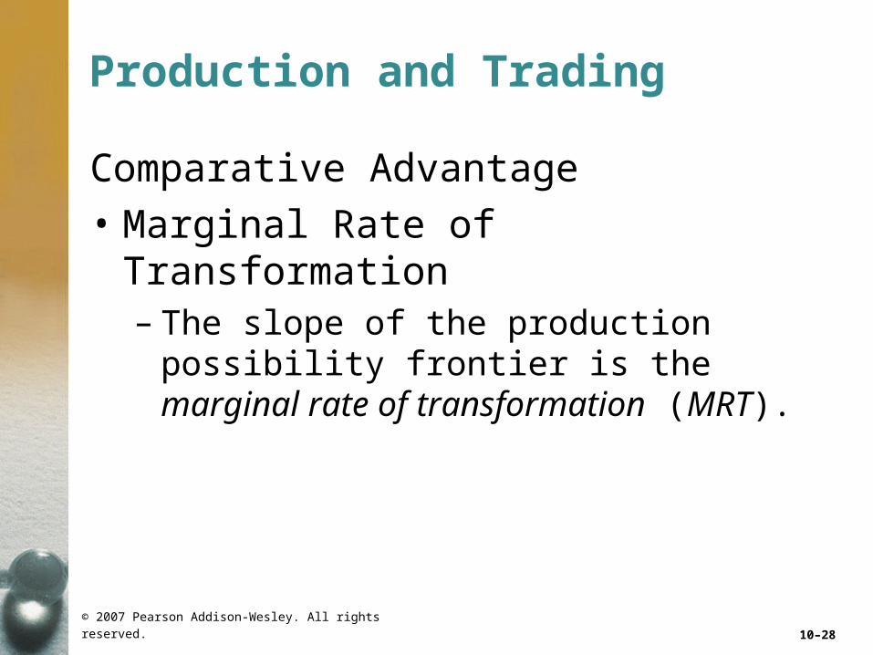
Comparative Advantage
• Marginal Rate of Transformation– The slope of the production possibility
frontier is the marginal rate of transformation (MRT).
© 2007 Pearson Addison-Wesley. All rights reserved. 10–29
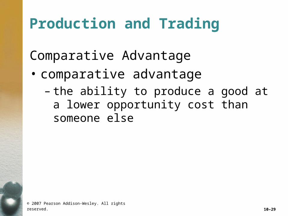
Production and Trading
Comparative Advantage
• comparative advantage– the ability to produce a good at a lower
opportunity cost than someone else

© 2007 Pearson Addison-Wesley. All rights reserved. 10–30
Production and Trading
Comparative Advantage
• Benefits of Trade– Because of the difference in their marginal
rates of transformation, Jane and Denise can benefit from a trade.

© 2007 Pearson Addison-Wesley. All rights reserved. 10–31
Production and Trading
• Comparative Advantage and Production Possibility Frontiers.
a) Jane’s production possibility frontier, , shows that in a day, she can produce 6 cords of firewood or 3 candy bars or any combination of the two. Her marginal rate of transformation (MRT) is -2.
jPPF

© 2007 Pearson Addison-Wesley. All rights reserved. 10–32
Production and Trading
b) Denise’s production possibility frontier, , has an MRT of .
c) Their joint production possibility frontier, PPF, has a kink at 6 cords of firewood (produced by Jane) and 6 candy bars (produced by Denise) and is concave to the origin.
dPPF1
2

© 2007 Pearson Addison-Wesley. All rights reserved. 10–33
Figure 10.6 Comparative Advantage and Production Possibility Frontiers
PPFd
Candy, Bars
3
2
(b) Denise
1
62
MRT = – 1–2
MRT = –2
6
PPFj
Candy, Bars
2
(a) Jane
1
2 3
PPF
MRT =–2(Jane)
Candy, Bars
6
9
(c) Joint Production
1
96
MRT = – (Denise)1–2
1

© 2007 Pearson Addison-Wesley. All rights reserved. 10–34
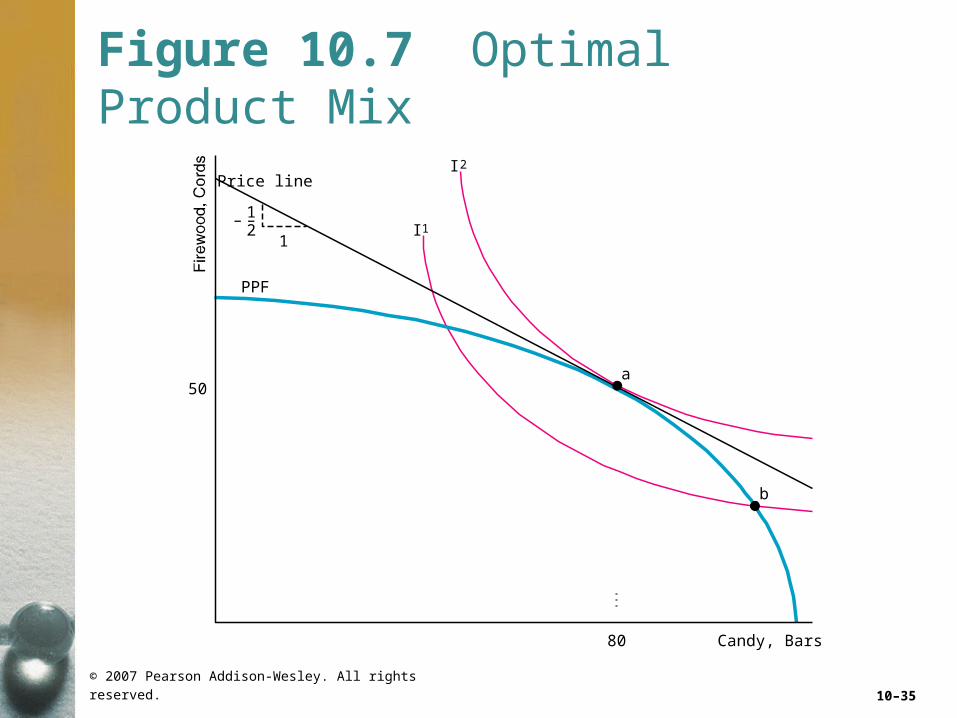
Comparative Advantage
• Optimal Product Mix.– The optimal product mix, , could be
determined by maximizing an individual’s utility by picking the allocation for which an indifference curve is tangent to the production possibility frontier.
– It could also be determined by picking the allocation where the relative competitive price, , equals the slope of the PPF.
a
/c fp p
© 2007 Pearson Addison-Wesley. All rights reserved. 10–35
Figure 10.7 Optimal Product Mix
I 1
I 2
Price line
PPF
1
80
50
Candy, Bars
a
b
1–2
–

© 2007 Pearson Addison-Wesley. All rights reserved. 10–36
Comparative Advantage
• The marginal rate of transformation along this smooth PPF tells us about the marginal cost of producing one good relative to the marginal cost of producing the other good.
c
w
MCMRT
MC
© 2007 Pearson Addison-Wesley. All rights reserved. 10–37
Comparative Advantage
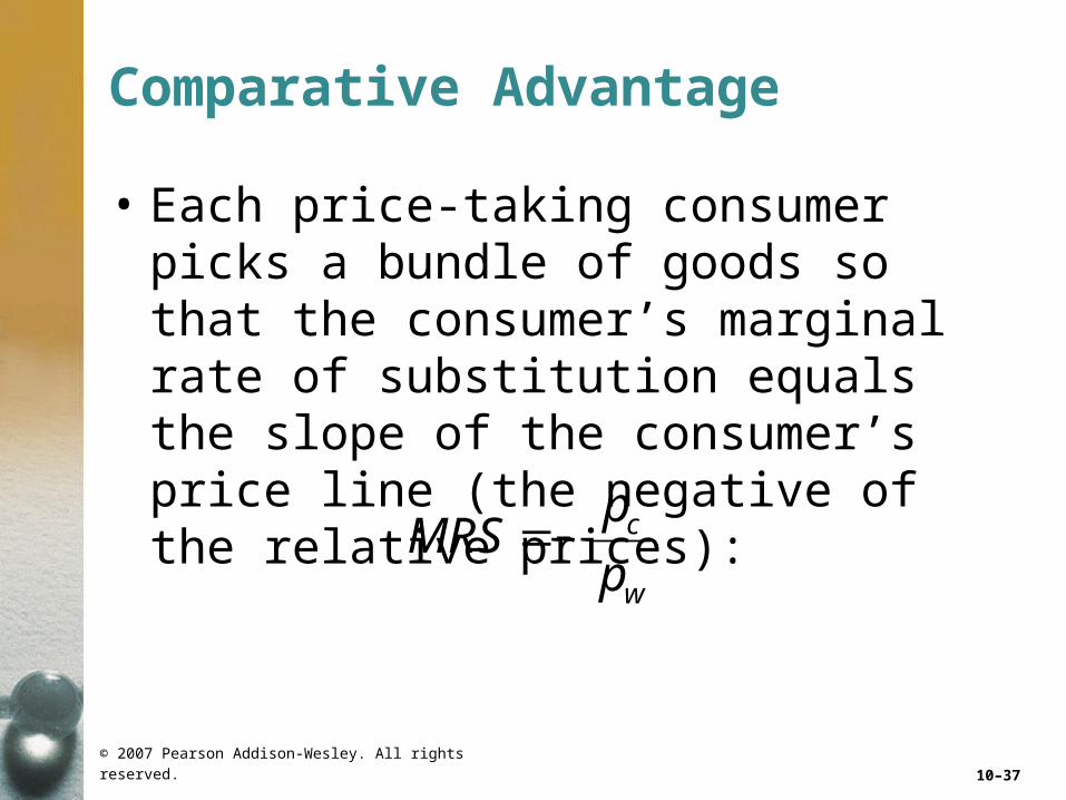
• Each price-taking consumer picks a bundle of goods so that the consumer’s marginal rate of substitution equals the slope of the consumer’s price line (the negative of the relative prices):
c
w
pMRS
p

© 2007 Pearson Addison-Wesley. All rights reserved. 10–38
Comparative Advantage
• If candy and wood are sold by competitive firms, and in the competitive equilibrium, the MRS equals the relative prices, which equals the MRT:
w wp MCc cp MC
c
w
pMRS MRT
p
© 2007 Pearson Addison-Wesley. All rights reserved. 10–39
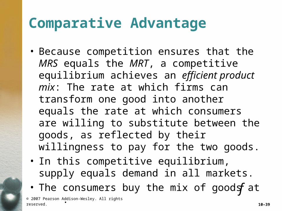
Comparative Advantage
• Because competition ensures that the MRS equals the MRT, a competitive equilibrium achieves an efficient product mix: The rate at which firms can transform one good into another equals the rate at which consumers are willing to substitute between the goods, as reflected by their willingness to pay for the two goods.
• In this competitive equilibrium, supply equals demand in all markets.
• The consumers buy the mix of goods at .f

© 2007 Pearson Addison-Wesley. All rights reserved. 10–40
Figure 10.8 Competitive Equilibrium
Ij
Id
Jane’s candy
Price line
Price line
PPF
40
40
1
1–2
–
1
80
40
20 30
50
Candy, Bars0j
f
a
1–2
–
Denise’s candy

© 2007 Pearson Addison-Wesley. All rights reserved. 10–41
Efficiency and Equity
• Role of the Government– By altering the efficiency with which goods
are produced and distributed and the endowment of resources, governments help determine how much is produced and how goods are allocated.
– By redistributing endowments or by refusing to do so, governments, at least implicitly, are making value judgments about which members of society should get relatively more of society’s goodies.
© 2007 Pearson Addison-Wesley. All rights reserved. 10–42
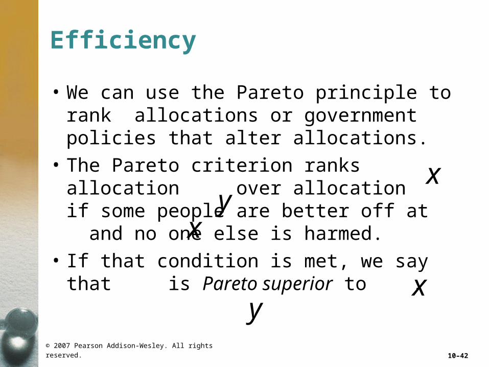
Efficiency
• We can use the Pareto principle to rank allocations or government policies that alter allocations.
• The Pareto criterion ranks allocation over allocation if some people are better off at and no one else is harmed.
• If that condition is met, we say that is Pareto superior to .
xy
x
xy
© 2007 Pearson Addison-Wesley. All rights reserved. 10–43
Efficiency
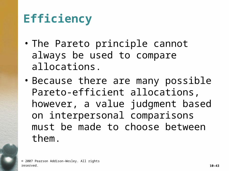
• The Pareto principle cannot always be used to compare allocations.
• Because there are many possible Pareto-efficient allocations, however, a value judgment based on interpersonal comparisons must be made to choose between them.

© 2007 Pearson Addison-Wesley. All rights reserved. 10–44
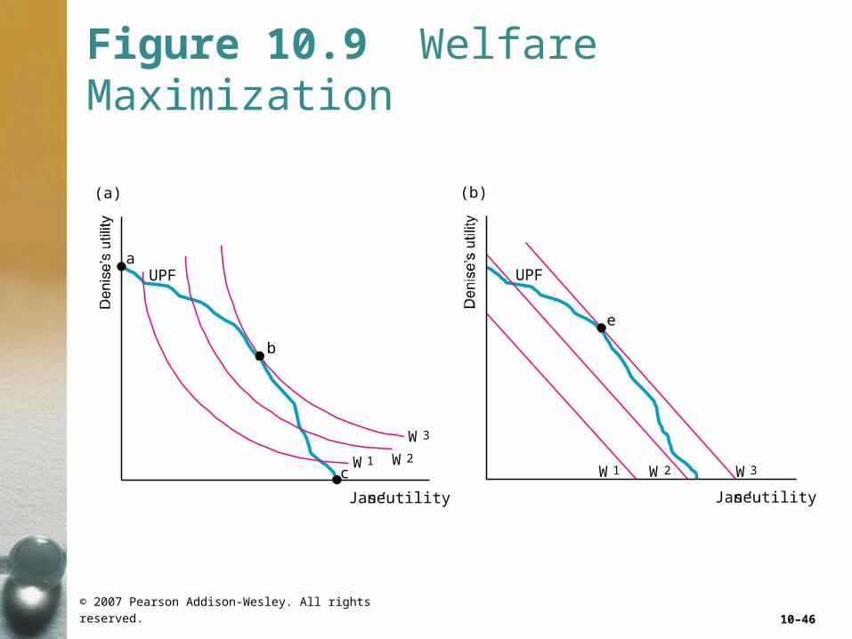
Equity
• If we are unwilling to use the Pareto principle or if that criterion does not allow us to rank the relevant allocations, we must make additional value judgments to rank these allocations.
• A way to summarize these value judgments is to use a social welfare function that combines various consumers’ utilities to provide a collective ranking of allocations.

© 2007 Pearson Addison-Wesley. All rights reserved. 10–45
Equity
• Who decides on the welfare function?
• In most countries, government leaders make decisions about which allocations are most desirable.
© 2007 Pearson Addison-Wesley. All rights reserved. 10–46
Figure 10.9 Welfare Maximization
UPF
c
a
b
(a)
Jane’s utility
W 1 W 2
W 3
UPF
e
(b)
Jane’s utility
W 1 W 2 W 3

© 2007 Pearson Addison-Wesley. All rights reserved. 10–47
Equity• Voting.
– In a democracy, important government policies that determine the allocation of goods are made by voting.
– Such democratic decision making is often difficult because people fundamentally disagree on how issues should be resolved and which groups of people should be favored.

© 2007 Pearson Addison-Wesley. All rights reserved. 10–48
Equity
• Unfortunately, sometimes voting does not work well, and the resulting social ordering of allocations is not transitive.

© 2007 Pearson Addison-Wesley. All rights reserved. 10–49
Equity
• Arrow’s Impossibility Theorem.
• Arrow suggested that a socially desirable decision making system, or social welfare function, should satisfy the following criteria:– Social preferences should be complete
(Chapter 4) and transitive, like individual preferences.

© 2007 Pearson Addison-Wesley. All rights reserved. 10–50
Equity
– If everyone prefers Allocation to Allocation , should be socially preferred to .
– Society’s ranking of and should depend only on individual’s ordering of these two allocations, not on how they rank other alternatives.
– Dictatorship is not allowed; social preferences must not reflect the preferences of only a single individual.
ab a
ba b

© 2007 Pearson Addison-Wesley. All rights reserved. 10–51
Equity
• Although each of these criteria seems reasonable—indeed, innocuous—Arrow proved that it is impossible to find a social decision-making rule that always satisfies all of these criteria.
© 2007 Pearson Addison-Wesley. All rights reserved. 10–52
Equity
• Social Welfare Functions.– How would you rank various allocations if
you were asked to vote?
• Jeremy Bentham (1748-1832) and his followers (including John Stuart Mill), the utilitarian philosophers, suggested that society should maximize the sum of the utilities of all members of society.
© 2007 Pearson Addison-Wesley. All rights reserved. 10–53
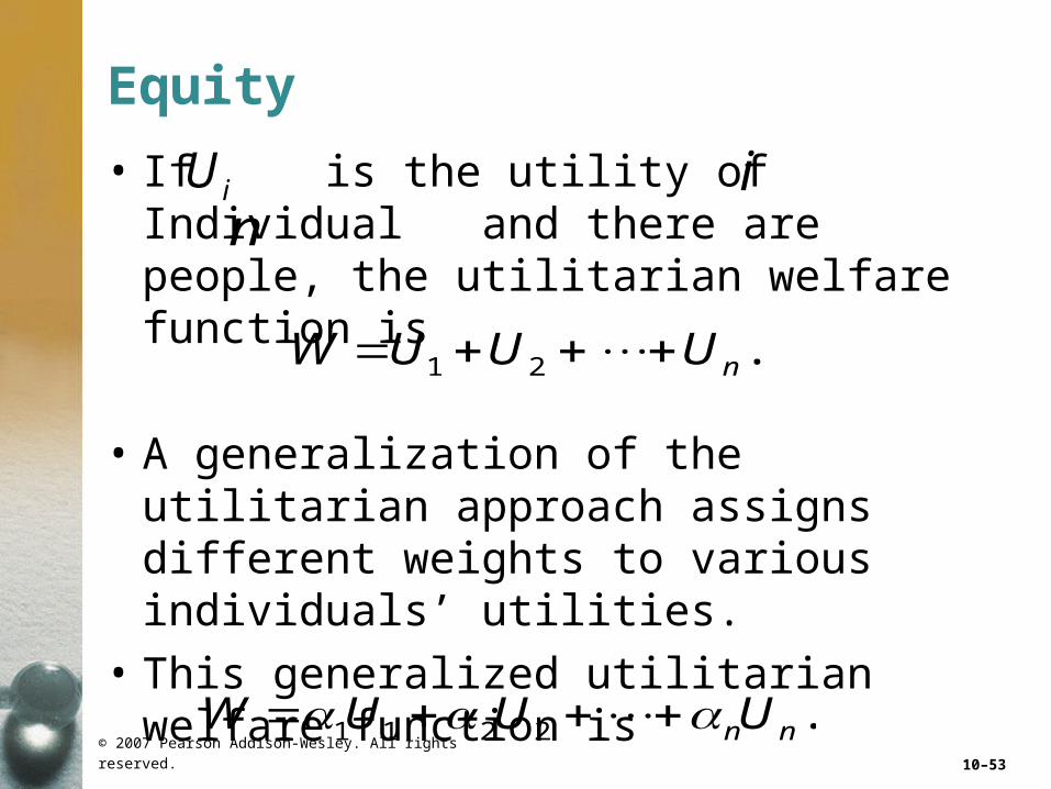
Equity
• If is the utility of Individual and there are people, the utilitarian welfare function is
• A generalization of the utilitarian approach assigns different weights to various individuals’ utilities.
• This generalized utilitarian welfare function is
iUn
i
1 2 . nW U U U
1 1 2 2 . n nW U U U
© 2007 Pearson Addison-Wesley. All rights reserved. 10–54
Equity
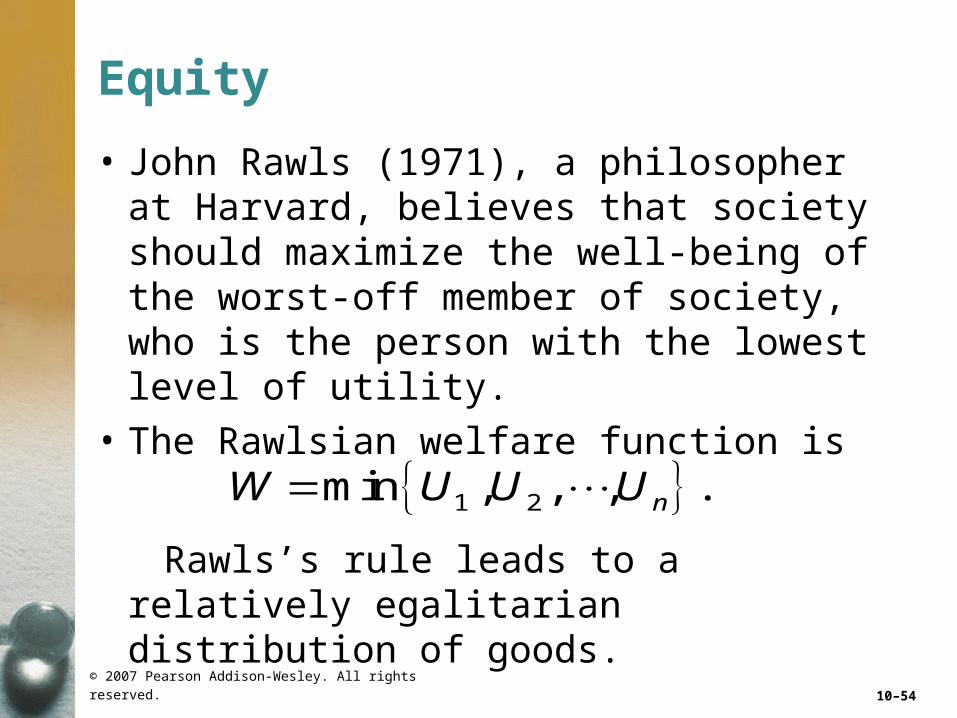
• John Rawls (1971), a philosopher at Harvard, believes that society should maximize the well-being of the worst-off member of society, who is the person with the lowest level of utility.
• The Rawlsian welfare function is
Rawls’s rule leads to a relatively egalitarian distribution of goods.
1 2min , , , . nW U U U

© 2007 Pearson Addison-Wesley. All rights reserved. 10–55
Efficiency Versus Equity
• Given a particular social welfare function, society might prefer an inefficient allocation to an efficient one.
© 2007 Pearson Addison-Wesley. All rights reserved. 10–56
Efficiency Versus Equity
• Competitive equilibrium may not be very equitable even though it is Pareto efficient.
• Consequently, societies that believe in equitable may tax the rich to give to the poor.
• If the money taken from the rich is given directly to the poor, society moves from one Pareto-efficient allocation to another.
© 2007 Pearson Addison-Wesley. All rights reserved. 10–57
Efficiency Versus Equity
• Unfortunately, there is frequently a conflict between a society’s goal of efficiency and the goal of achieving an equitable allocation.
• Even when the government redistributes money form one group to another, there are significant costs to this redistribution.