chapter sequence processing with recurrent networksjurafsky/slp3/9.pdf · niscent of the markov...
TRANSCRIPT
Speech and Language Processing. Daniel Jurafsky & James H. Martin. Copyright c© 2018. All
rights reserved. Draft of September 23, 2018.
CHAPTER
9 Sequence Processing withRecurrent Networks
Time will explain.Jane Austin, Persuasion
In Chapter 7, we explored feedforward neural networks along with their applicationsto neural language models and text classification. In the case of language models,we saw that such networks can be trained to make predictions about the next word ina sequence given a limited context of preceding words — an approach that is remi-niscent of the Markov approach to language modeling discussed in Chapter 3. Thesemodels operated by accepting a small fixed-sized window of tokens as input; longersequences are processed by sliding this window over the input making incrementalpredictions, with the end result being a sequence of predictions spanning the input.Fig. 9.1, reproduced here from Chapter 7, illustrates this approach with a windowof size 3. Here, we’re predicting which word will come next given the window theground there. Subsequent words are predicted by sliding the window forward oneword at a time.
Unfortunately, the sliding window approach is problematic for a number of rea-sons. First, it shares the primary weakness of Markov approaches in that it limitsthe context from which information can be extracted; anything outside the contextwindow has no impact on the decision being made. This is problematic since thereare many language tasks that require access to information that can be arbitrarily dis-tant from the point at which processing is happening. Second, the use of windowsmakes it difficult for networks to learn systematic patterns arising from phenomenalike constituency. For example, in Fig. 9.1 the phrase the ground appears twice indifferent windows: once, as shown, in the first and second positions in the window,and in in the preceding step in the second and third slots, thus forcing the networkto learn two separate patterns for a single constituent.
The subject of this chapter is recurrent neural networks, a class of networksdesigned to address these problems by processing sequences explicitly as sequences,allowing us to handle variable length inputs without the use of arbitrary fixed-sizedwindows.
9.1 Simple Recurrent Networks
A recurrent neural network is any network that contains is a cycle within its networkconnections. That is, any network where the value of a unit is directly, or indirectly,dependent on its own output as an input. In general, such networks are difficult toreason about, and to train. However, within the general class of recurrent networks

2 CHAPTER 9 • SEQUENCE PROCESSING WITH RECURRENT NETWORKS
h1 h2
y1
h3 hdh…
…
U
W
y42 y|V|
Projection layer 1⨉3dconcatenated embeddings
for context words
Hidden layer
Output layer P(w|u) …
in thehole... ...ground there lived
word 42embedding for
word 35embedding for
word 9925embedding for
word 45180
wt-1wt-2 wtwt-3
dh⨉3d
1⨉dh
|V|⨉dh P(wt=V42|wt-3,wt-2,wt-3)
1⨉|V|
Figure 9.1 A simplified view of a feedforward neural language model moving through a text. At eachtimestep t the network takes the 3 context words, converts each to a d-dimensional embeddings, and con-catenates the 3 embeddings together to get the 1×Nd unit input layer x for the network.
there are constrained architectures that have proven to be extremely useful whenapplied to language problems. In this section, we’ll introduce a class of recurrentnetworks referred to as Simple Recurrent Networks (SRNs) or Elman Networks
SimpleRecurrentNetworksElmanNetworks (Elman, 1990). These networks are useful in their own right, and will serve as the
basis for more complex approaches to be discussed later in this chapter and again inChapter 22.
Fig. 9.2 abstractly illustrates the recurrent structure of an SRN. As with ordinaryfeed-forward networks, an input vector representing the current input element, xt ,is multiplied by a weight matrix and then passed through an activation function tocompute an activation value for a layer of hidden of units. This hidden layer is,in turn, used to calculate a corresponding output, yt . Sequences are processed by
ht
yt
xt
Figure 9.2 Simple recurrent neural network after Elman (Elman, 1990). The hidden layerincludes a recurrent connection as part of its input. That is, the activation value of the hiddenlayer depends on the current input as well as the activation value of the hidden layer from theprevious timestep.
9.1 • SIMPLE RECURRENT NETWORKS 3
U
V
W
yt
xt
ht
ht-1
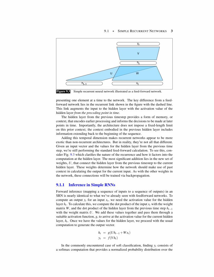
Figure 9.3 Simple recurrent neural network illustrated as a feed-forward network.
presenting one element at a time to the network. The key difference from a feed-forward network lies in the recurrent link shown in the figure with the dashed line.This link augments the input to the hidden layer with the activation value of thehidden layer from the preceding point in time.
The hidden layer from the previous timestep provides a form of memory, orcontext, that encodes earlier processing and informs the decisions to be made at laterpoints in time. Importantly, the architecture does not impose a fixed-length limiton this prior context; the context embodied in the previous hidden layer includesinformation extending back to the beginning of the sequence.
Adding this temporal dimension makes recurrent networks appear to be moreexotic than non-recurrent architectures. But in reality, they’re not all that different.Given an input vector and the values for the hidden layer from the previous timestep, we’re still performing the standard feed-forward calculation. To see this, con-sider Fig. 9.3 which clarifies the nature of the recurrence and how it factors into thecomputation at the hidden layer. The most significant addition lies in the new set ofweights, U , that connect the hidden layer from the previous timestep to the currenthidden layer. These weights determine how the network should make use of pastcontext in calculating the output for the current input. As with the other weights inthe network, these connections will be trained via backpropagation.
9.1.1 Inference in Simple RNNsForward inference (mapping a sequence of inputs to a sequence of outputs) in anSRN is nearly identical to what we’ve already seen with feedforward networks. Tocompute an output yt for an input xt , we need the activation value for the hiddenlayer ht . To calculate this, we compute the dot product of the input xt with the weightmatrix W , and the dot product of the hidden layer from the previous time step ht−1with the weight matrix U . We add these values together and pass them through asuitable activation function, g, to arrive at the activation value for the current hiddenlayer, ht . Once we have the values for the hidden layer, we proceed with the usualcomputation to generate the output vector.
ht = g(Uht−1 +Wxt)
yt = f (V ht)
In the commonly encountered case of soft classification, finding yt consists ofa softmax computation that provides a normalized probability distribution over the

4 CHAPTER 9 • SEQUENCE PROCESSING WITH RECURRENT NETWORKS
U
V
W
U
V
W
U
V
W
x1
x2
x3y1
y2
y3
h1
h3
h2
h0
Figure 9.4 A simple recurrent neural network shown unrolled in time. Network layers are copied for eachtimestep, while the weights U , V and W are shared in common across all timesteps.
possible output classes.
yt = softmax(V ht)
The sequential nature of simple recurrent networks can be illustrated by un-rolling the network in time as is shown in Fig. 9.4. In figures such as this, thevarious layers of units are copied for each time step to illustrate that they will havediffering values over time. However the weights themselves are shared across thevarious timesteps. Finally, the fact that the computation at time t requires the valueof the hidden layer from time t−1 mandates an incremental inference algorithm thatproceeds from the start of the sequence to the end as shown in Fig. 9.5.
function FORWARDRNN(x, network) returns output sequence y
h0←0for i←1 to LENGTH(x) do
hi←g(U hi−1 + W xi)yi← f (V hi)
return y
Figure 9.5 Forward inference in a simple recurrent network.
9.1.2 TrainingAs we did with feed-forward networks, we’ll use a training set, a loss function, andbackpropagation to adjust the sets of weights in these recurrent networks. As shownin Fig. 9.3, we now have 3 sets of weights to update: W , the weights from the input
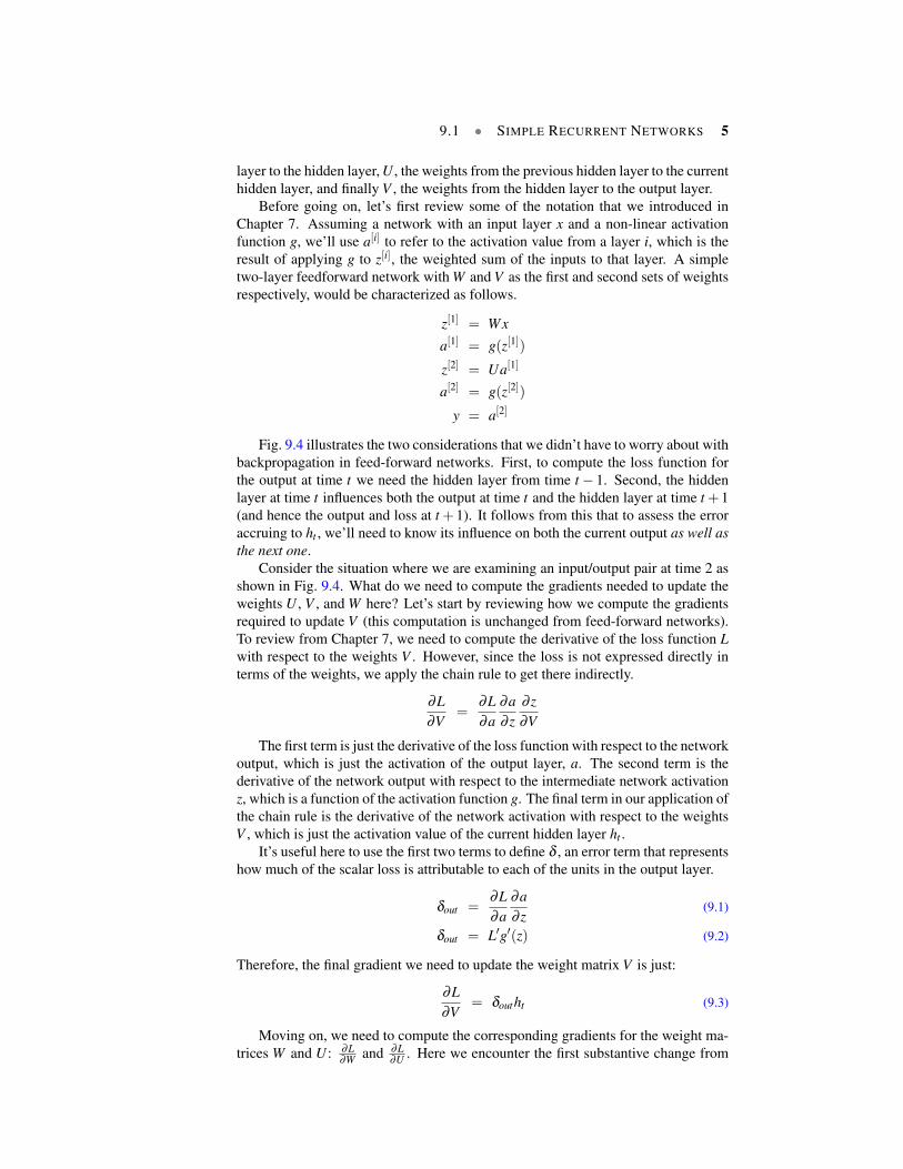
9.1 • SIMPLE RECURRENT NETWORKS 5
layer to the hidden layer, U , the weights from the previous hidden layer to the currenthidden layer, and finally V , the weights from the hidden layer to the output layer.
Before going on, let’s first review some of the notation that we introduced inChapter 7. Assuming a network with an input layer x and a non-linear activationfunction g, we’ll use a[i] to refer to the activation value from a layer i, which is theresult of applying g to z[i], the weighted sum of the inputs to that layer. A simpletwo-layer feedforward network with W and V as the first and second sets of weightsrespectively, would be characterized as follows.
z[1] = Wx
a[1] = g(z[1])
z[2] = Ua[1]
a[2] = g(z[2])
y = a[2]
Fig. 9.4 illustrates the two considerations that we didn’t have to worry about withbackpropagation in feed-forward networks. First, to compute the loss function forthe output at time t we need the hidden layer from time t− 1. Second, the hiddenlayer at time t influences both the output at time t and the hidden layer at time t +1(and hence the output and loss at t +1). It follows from this that to assess the erroraccruing to ht , we’ll need to know its influence on both the current output as well asthe next one.
Consider the situation where we are examining an input/output pair at time 2 asshown in Fig. 9.4. What do we need to compute the gradients needed to update theweights U , V , and W here? Let’s start by reviewing how we compute the gradientsrequired to update V (this computation is unchanged from feed-forward networks).To review from Chapter 7, we need to compute the derivative of the loss function Lwith respect to the weights V . However, since the loss is not expressed directly interms of the weights, we apply the chain rule to get there indirectly.
∂L∂V
=∂L∂a
∂a∂ z
∂ z∂V
The first term is just the derivative of the loss function with respect to the networkoutput, which is just the activation of the output layer, a. The second term is thederivative of the network output with respect to the intermediate network activationz, which is a function of the activation function g. The final term in our application ofthe chain rule is the derivative of the network activation with respect to the weightsV , which is just the activation value of the current hidden layer ht .
It’s useful here to use the first two terms to define δ , an error term that representshow much of the scalar loss is attributable to each of the units in the output layer.
δout =∂L∂a
∂a∂ z
(9.1)
δout = L′g′(z) (9.2)
Therefore, the final gradient we need to update the weight matrix V is just:
∂L∂V
= δoutht (9.3)
Moving on, we need to compute the corresponding gradients for the weight ma-trices W and U : ∂L
∂W and ∂L∂U . Here we encounter the first substantive change from
6 CHAPTER 9 • SEQUENCE PROCESSING WITH RECURRENT NETWORKS
U
V
W
U
V
W
U
V
W
x1
x2
x3y1
y2
y3
h1
h3
h2
h0
t1
t2
t3
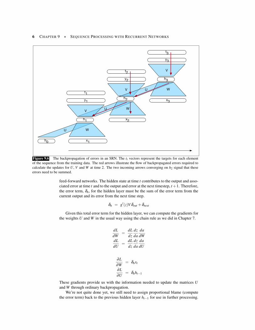
Figure 9.6 The backpropagation of errors in an SRN. The ti vectors represent the targets for each elementof the sequence from the training data. The red arrows illustrate the flow of backpropagated errors required tocalculate the updates for U , V and W at time 2. The two incoming arrows converging on h2 signal that theseerrors need to be summed.
feed-forward networks. The hidden state at time t contributes to the output and asso-ciated error at time t and to the output and error at the next timestep, t+1. Therefore,the error term, δh, for the hidden layer must be the sum of the error term from thecurrent output and its error from the next time step.
δh = g′(z)V δout +δnext
Given this total error term for the hidden layer, we can compute the gradients forthe weights U and W in the usual way using the chain rule as we did in Chapter 7.
dLdW
=dLdz
dzda
dadW
dLdU
=dLdz
dzda
dadU
∂L∂W
= δhxt
∂L∂U
= δhht−1
These gradients provide us with the information needed to update the matrices Uand W through ordinary backpropagation.
We’re not quite done yet, we still need to assign proportional blame (computethe error term) back to the previous hidden layer ht−1 for use in further processing.

9.1 • SIMPLE RECURRENT NETWORKS 7
function BACKPROPTHROUGHTIME(sequence, network) returns gradients for weightupdatesforward pass to gather the lossbackward pass compute error terms and assess blame
Figure 9.7 Backpropagation training through time. The forward pass computes the re-quired loss values at each time step. The backward pass computes the gradients using thevalues from the forward pass.
This involves backpropagating the error from δh to ht−1 proportionally based on theweights in U .
δnext = g′(z)Uδh (9.4)
At this point we have all the gradients needed to perform weight updates for eachof our three sets of weights. Note that in this simple case there is no need to back-propagate the error through W to the input x, since the input training data is assumedto be fixed. If we wished to update our input word or character embeddings wewould backpropagate the error through to them as well. We’ll discuss this more inSection 9.5.
Taken together, all of these considerations lead to a two-pass algorithm for train-ing the weights in SRNs. In the first pass, we perform forward inference, computinght , yt , and an loss at each step in time, saving the value of the hidden layer at eachstep for use at the next time step. In the second phase, we process the sequencein reverse, computing the required error terms gradients as we go, computing andsaving the error term for use in the hidden layer for each step backward.
Unfortunately, computing the gradients and updating weights for each item of asequence individually would be extremely time-consuming. Instead, much as we didwith mini-batch training in Chapter 7, we will accumulate gradients for the weightsincrementally over the sequence, and then use those accumulated gradients in per-forming weight updates.
9.1.3 Unrolled Networks as Computational GraphsWe used the unrolled network shown in Fig. 9.4 as a way to understand the dynamicbehavior of these networks over time. However, with modern computational frame-works and adequate computing resources, explicitly unrolling a recurrent networkinto a deep feed-forward computational graph is quite practical for word-by-wordapproaches to sentence-level processing. In such an approach, we provide a tem-plate that specifies the basic structure of the SRN, including all the necessary pa-rameters for the input, output, and hidden layers, the weight matrices, as well as theactivation and output functions to be used. Then, when provided with an input se-quence such as a training sentence, we can compile a feed-forward graph specific tothat input, and use that graph to perform forward inference or training via ordinarybackpropagation.
For applications that involve much longer input sequences, such as speech recog-nition, character-by-character sentence processing, or streaming of continuous in-puts, unrolling an entire input sequence may not be feasible. In these cases, we canunroll the input into manageable fixed-length segments and treat each segment as adistinct training item. This approach is called Truncated Backpropagation ThroughTime (TBTT).

8 CHAPTER 9 • SEQUENCE PROCESSING WITH RECURRENT NETWORKS
Janet will back
RNN
the bill
Figure 9.8 Part-of-speech tagging as sequence labeling with a simple RNN. Pre-trainedword embeddings serve as inputs and a softmax layer provides a probability distribution overthe part-of-speech tags as output at each time step.
9.2 Applications of RNNs
Simple recurrent networks have proven to be an effective approach to language mod-eling, sequence labeling tasks such as part-of-speech tagging, as well as sequenceclassification tasks such as sentiment analysis and topic classification. And as we’llsee in Chapter 22, they form the basic building blocks for sequence to sequenceapproaches to applications such as summarization and machine translation.
9.2.1 Generation with Neural Language Models[Coming soon]
9.2.2 Sequence LabelingIn sequence labeling, the network’s job is to assign a label to each element of asequence chosen from a small fixed set of labels. The canonical example of such atask is part-of-speech tagging, discussed in Chapter 8. In a recurrent network-basedapproach to POS tagging, inputs are words and the outputs are tag probabilitiesgenerated by a softmax layer over the POS tagset, as illustrated in Fig. 9.8.
In this figure, the inputs at each time step are pre-trained word embeddings cor-responding to the input tokens. The RNN block is an abstraction that representsan unrolled simple recurrent network consisting of an input layer, hidden layer, andoutput layer at each time step, as well as the shared U , V and W weight matrices thatcomprise the network. The outputs of the network at each time step represent thedistribution over the POS tagset generated by a softmax layer. To generate an actualtag sequence as output, we can run forward inference over the input sequence andselect the most likely tag from the softmax at each step. Since we’re using a softmaxlayer to generate the probability distribution over the output tagset at each timestep,we’ll rely on the cross entropy loss introduced in Chapter 7 to train the network.
A closely related, and extremely useful, application of sequence labeling is tofind and classify spans of text corresponding to items of interest in some task do-main. An example of such a task is named entity recognition — the problem ofnamed entity
recognition
9.2 • APPLICATIONS OF RNNS 9
finding all the spans in a text that correspond to names of people, places or organi-zations (a problem we’ll study in gory detail in Chapter 17).
To turn a problem like this into a per-word sequence labeling task, we’ll use atechnique called IOB encoding (Ramshaw and Marcus, 1995). In its simplest form,we’ll label any token that begins a span of interest with the label B, tokens that occurinside a span are tagged with an I, and any tokens outside of any span of interest arelabeled O. Consider the following example:
(9.5) UnitedB
cancelledO
theO
flightO
fromO
DenverB
toO
SanB
Francisco.I
Here, the spans of interest are United, Denver and San Francisco.In applications where we are interested in more than one class of entity (e.g.,
finding and distinguishing names of people, locations, or organizations), we canspecialize the B and I tags to represent each of the more specific classes, thus ex-panding the tagset from 3 tags to 2 ∗N + 1 where N is the number of classes we’reinterested in.
(9.6) UnitedB-ORG
cancelledO
theO
flightO
fromO
DenverB-LOC
toO
SanB-LOC
Francisco.I-LOC
With such an encoding, the inputs are the usual word embeddings and the outputconsistes of a sequence of softmax distributions over the tags at each point in thesequence.
9.2.3 Viterbi and Conditional Random Fields (CRFs)As we saw with applying logistic regression to part-of-speech tagging, choosing themaximum probability label for each element in a sequence does not necessarily re-sult in an optimal (or even very good) tag sequence. In the case of IOB tagging, itdoesn’t even guarantee that the resulting sequence will be well-formed. For exam-ple, nothing in approach described in the last section prevents an output sequencefrom containing an I following an O, even though such a transition is illegal. Simi-larly, when dealing with multiple classes nothing would prevent an I-LOC tag fromfollowing a B-PER tag.
A simple solution to this problem is to use combine the sequence of probabilitydistributions provided by the softmax outputs with a tag-level language model as wedid with MEMMs in Chapter 8. Thereby allowing the use of the Viterbi algorithmto select the most likely tag sequence.
[Or a CRF layer... Coming soon]
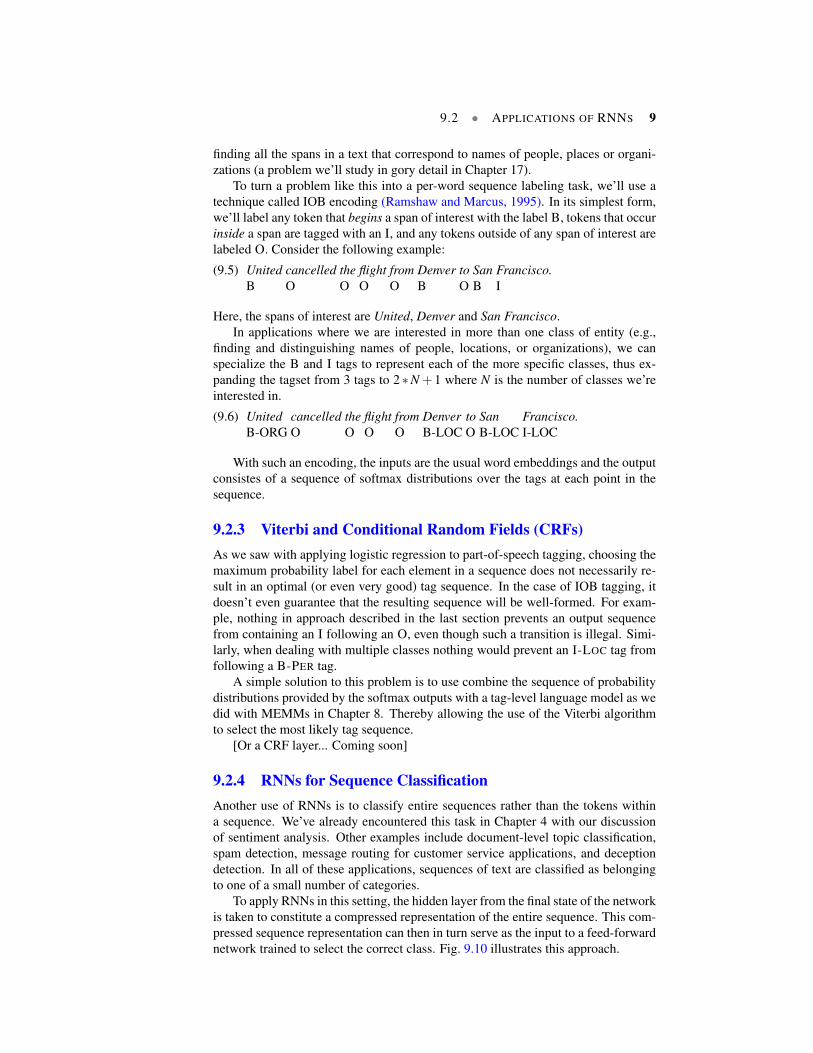
9.2.4 RNNs for Sequence ClassificationAnother use of RNNs is to classify entire sequences rather than the tokens withina sequence. We’ve already encountered this task in Chapter 4 with our discussionof sentiment analysis. Other examples include document-level topic classification,spam detection, message routing for customer service applications, and deceptiondetection. In all of these applications, sequences of text are classified as belongingto one of a small number of categories.
To apply RNNs in this setting, the hidden layer from the final state of the networkis taken to constitute a compressed representation of the entire sequence. This com-pressed sequence representation can then in turn serve as the input to a feed-forwardnetwork trained to select the correct class. Fig. 9.10 illustrates this approach.
10 CHAPTER 9 • SEQUENCE PROCESSING WITH RECURRENT NETWORKS
x1 x2 x3 xn
RNN
hn
Softmax
Figure 9.9 Sequence classification using a simple RNN combined with a feedforward net-work.
Note that in this approach, there are no intermediate outputs for the items in thesequence preceding the last element, and therefore there are no loss terms associ-ated with those individual items. Instead, the loss used to train the network weightsis based on the loss from the final classification task. Specifically, we use the outputfrom the softmax layer from the final classifier along with a cross-entropy loss func-tion to drive our network training. The loss is backpropagated all the way throughthe weights in the feedforward classifier through to its input, and then through to thethree sets of weights in the RNN as described earlier in Section 9.1.2. This combina-tion of a simple recurrent network with a feedforward classifier is our first exampleof a deep neural network.
9.3 Deep Networks: Stacked and Bidirectional RNNs
As suggested by the sequence classification architecture shown in Fig. 9.9, recur-rent networks are in fact quite flexible. Combining the feedforward nature of un-rolled computational graphs with vectors as common inputs and outputs, complexnetworks can be treated as modules that can be combined in creative ways. Thissection introduces two of the more common network architectures used in languageprocessing with RNNs.
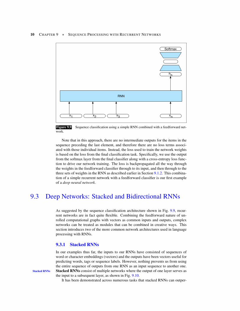
9.3.1 Stacked RNNsIn our examples thus far, the inputs to our RNNs have consisted of sequences ofword or character embeddings (vectors) and the outputs have been vectors useful forpredicting words, tags or sequence labels. However, nothing prevents us from usingthe entire sequence of outputs from one RNN as an input sequence to another one.Stacked RNNs consist of multiple networks where the output of one layer serves asStacked RNNs
the input to a subsequent layer, as shown in Fig. 9.10.It has been demonstrated across numerous tasks that stacked RNNs can outper-
9.3 • DEEP NETWORKS: STACKED AND BIDIRECTIONAL RNNS 11
y1 y2 y3yn
x1 x2 x3 xn
RNN 1
RNN 3
RNN 2
Figure 9.10 Stacked recurrent networks. The output of a lower level serves as the input tohigher levels with the output of the last network serving as the final output.
form single-layer networks. One reason for this success has to do with the networksability to induce representations at differing levels of abstraction across layers. Justas the early stages of the human visual system detects edges that are then used forfinding larger regions and shapes, the initial layers of stacked networks can inducerepresentations that serve as useful abstractions for further layers — representationsthat might prove difficult to induce in a single RNN.
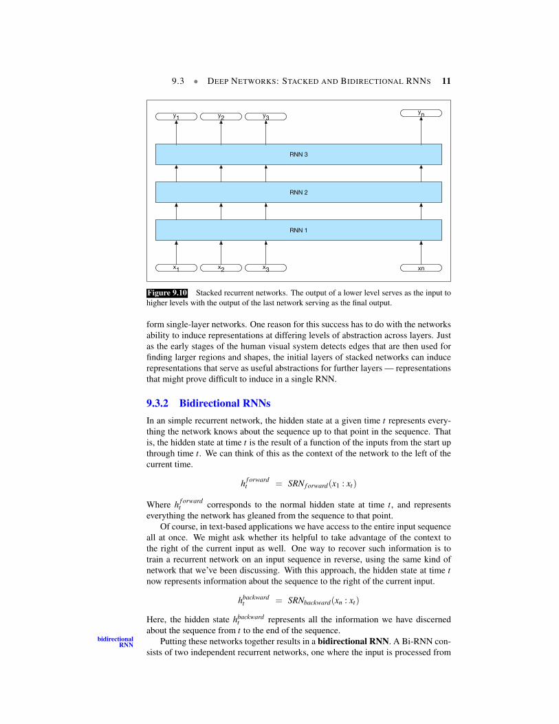
9.3.2 Bidirectional RNNsIn an simple recurrent network, the hidden state at a given time t represents every-thing the network knows about the sequence up to that point in the sequence. Thatis, the hidden state at time t is the result of a function of the inputs from the start upthrough time t. We can think of this as the context of the network to the left of thecurrent time.
h f orwardt = SRN f orward(x1 : xt)
Where h f orwardt corresponds to the normal hidden state at time t, and represents
everything the network has gleaned from the sequence to that point.Of course, in text-based applications we have access to the entire input sequence
all at once. We might ask whether its helpful to take advantage of the context tothe right of the current input as well. One way to recover such information is totrain a recurrent network on an input sequence in reverse, using the same kind ofnetwork that we’ve been discussing. With this approach, the hidden state at time tnow represents information about the sequence to the right of the current input.
hbackwardt = SRNbackward(xn : xt)
Here, the hidden state hbackwardt represents all the information we have discerned
about the sequence from t to the end of the sequence.Putting these networks together results in a bidirectional RNN. A Bi-RNN con-bidirectional
RNNsists of two independent recurrent networks, one where the input is processed from
12 CHAPTER 9 • SEQUENCE PROCESSING WITH RECURRENT NETWORKS
y1
x1 x2 x3 xn
RNN 1 (Left to Right)
RNN 2 (Right to Left)
+
y2
+
y3
+
yn
+
Figure 9.11 A bidirectional RNN. Separate models are trained in the forward and backwarddirections with the output of each model at each time point concatenated to represent the stateof affairs at that point in time. The box wrapped around the forward and backward networkemphasizes the modular nature of this architecture.
the start to the end, and the other from the end to the start. We can then combine theoutputs of the two networks into a single representation that captures the both theleft and right contexts of an input at each point in time.
ht = h f orwardt ⊕hbackward
t (9.7)
Fig. 9.11 illustrates a bidirectional network where the outputs of the forward andbackward pass are concatenated. Other simple ways to combine the forward andbackward contexts include element-wise addition or multiplication. The output ateach step in time thus captures information to the left and to the right of the currentinput. In sequence labeling applications, these concatenated outputs can serve as thebasis for a local labeling decision.
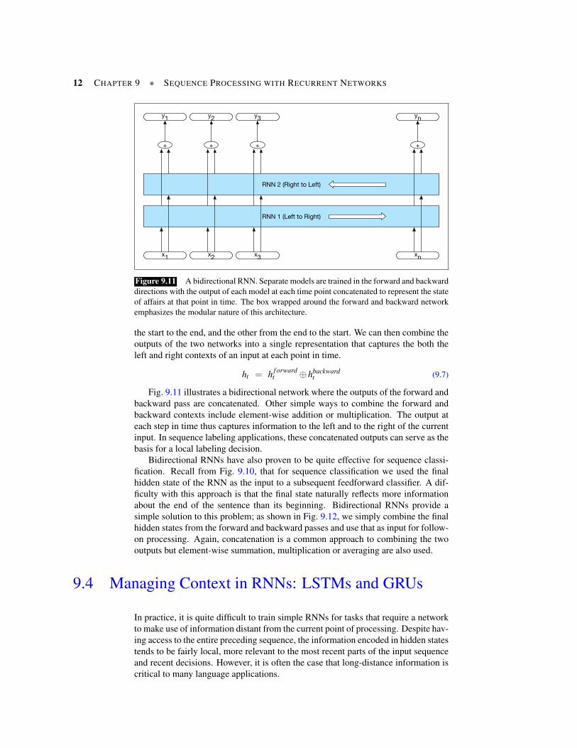
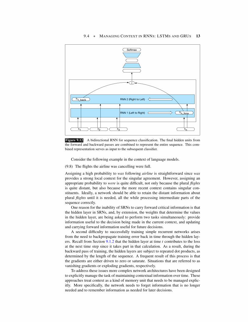
Bidirectional RNNs have also proven to be quite effective for sequence classi-fication. Recall from Fig. 9.10, that for sequence classification we used the finalhidden state of the RNN as the input to a subsequent feedforward classifier. A dif-ficulty with this approach is that the final state naturally reflects more informationabout the end of the sentence than its beginning. Bidirectional RNNs provide asimple solution to this problem; as shown in Fig. 9.12, we simply combine the finalhidden states from the forward and backward passes and use that as input for follow-on processing. Again, concatenation is a common approach to combining the twooutputs but element-wise summation, multiplication or averaging are also used.
9.4 Managing Context in RNNs: LSTMs and GRUs
In practice, it is quite difficult to train simple RNNs for tasks that require a networkto make use of information distant from the current point of processing. Despite hav-ing access to the entire preceding sequence, the information encoded in hidden statestends to be fairly local, more relevant to the most recent parts of the input sequenceand recent decisions. However, it is often the case that long-distance information iscritical to many language applications.
9.4 • MANAGING CONTEXT IN RNNS: LSTMS AND GRUS 13
x1 x2 x3 xn
RNN 1 (Left to Right)
RNN 2 (Right to Left)
+
hn_forw
h1_back
Softmax
Figure 9.12 A bidirectional RNN for sequence classification. The final hidden units fromthe forward and backward passes are combined to represent the entire sequence. This com-bined representation serves as input to the subsequent classifier.
Consider the following example in the context of language models.
(9.8) The flights the airline was cancelling were full.
Assigning a high probability to was following airline is straightforward since wasprovides a strong local context for the singular agreement. However, assigning anappropriate probability to were is quite difficult, not only because the plural flightsis quite distant, but also because the more recent context contains singular con-stituents. Ideally, a network should be able to retain the distant information aboutplural flights until it is needed, all the while processing intermediate parts of thesequence correctly.
One reason for the inability of SRNs to carry forward critical information is thatthe hidden layer in SRNs, and, by extension, the weights that determine the valuesin the hidden layer, are being asked to perform two tasks simultaneously: provideinformation useful to the decision being made in the current context, and updatingand carrying forward information useful for future decisions.
A second difficulty to successfully training simple recurrent networks arisesfrom the need to backpropagate training error back in time through the hidden lay-ers. Recall from Section 9.1.2 that the hidden layer at time t contributes to the lossat the next time step since it takes part in that calculation. As a result, during thebackward pass of training, the hidden layers are subject to repeated dot products, asdetermined by the length of the sequence. A frequent result of this process is thatthe gradients are either driven to zero or saturate. Situations that are referred to asvanishing gradients or exploding gradients, respectively.
To address these issues more complex network architectures have been designedto explicitly manage the task of maintaining contextual information over time. Theseapproaches treat context as a kind of memory unit that needs to be managed explic-itly. More specifically, the network needs to forget information that is no longerneeded and to remember information as needed for later decisions.
14 CHAPTER 9 • SEQUENCE PROCESSING WITH RECURRENT NETWORKS
+
ost-1 if g
x tht-1
Y Y
Y
st
ht
Figure 9.13 A single LSTM memory unit displayed as a computation graph.
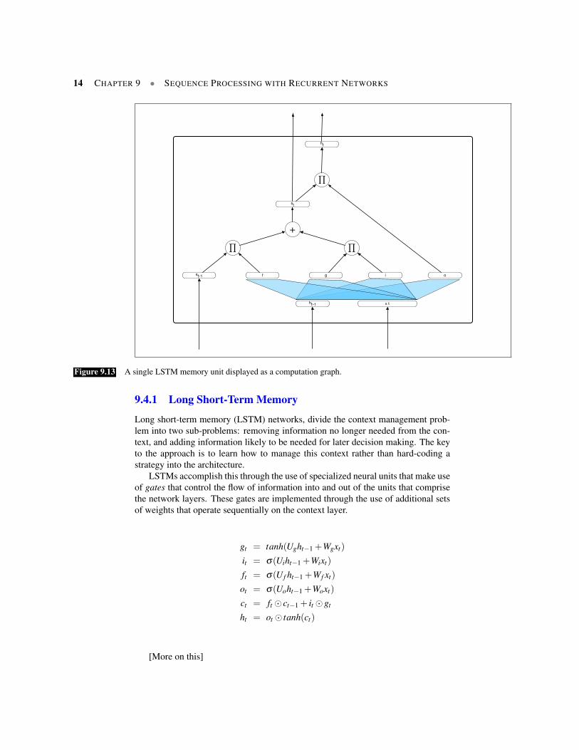
9.4.1 Long Short-Term Memory
Long short-term memory (LSTM) networks, divide the context management prob-lem into two sub-problems: removing information no longer needed from the con-text, and adding information likely to be needed for later decision making. The keyto the approach is to learn how to manage this context rather than hard-coding astrategy into the architecture.
LSTMs accomplish this through the use of specialized neural units that make useof gates that control the flow of information into and out of the units that comprisethe network layers. These gates are implemented through the use of additional setsof weights that operate sequentially on the context layer.
gt = tanh(Ught−1 +Wgxt)
it = σ(Uiht−1 +Wixt)
ft = σ(U f ht−1 +Wf xt)
ot = σ(Uoht−1 +Woxt)
ct = ft � ct−1 + it �gt
ht = ot � tanh(ct)
9.4 • MANAGING CONTEXT IN RNNS: LSTMS AND GRUS 15
h
x xt xtht-1
ht ht
ct-1
ct
ht-1 xt
ht
ct-1
ct
ht-1
(b)(a) (c) (d)
⌃
g
z
a
⌃
g
zLSTMUnit
GRUUnit
a
Figure 9.14 Basic neural units used in feed-forward, simple recurrent networks (SRN),long short-term memory (LSTM) and gate recurrent units.
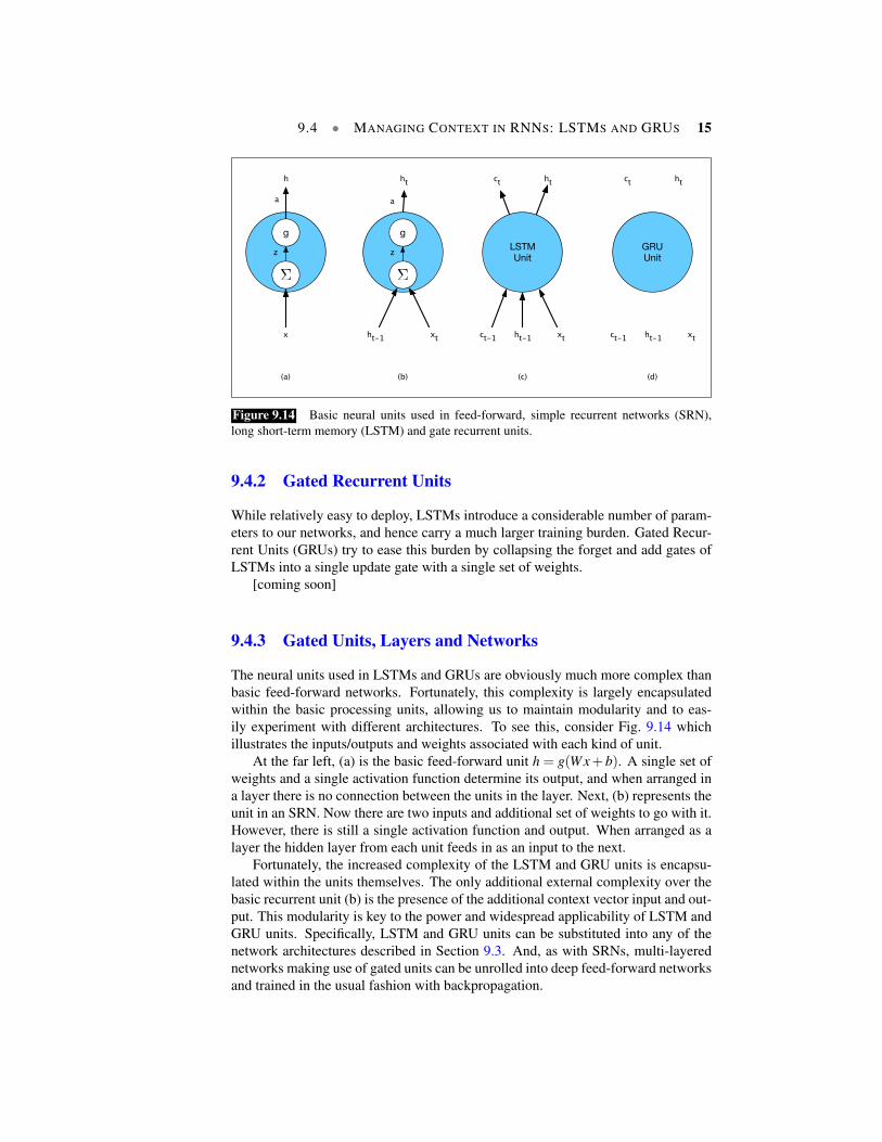
9.4.2 Gated Recurrent Units
While relatively easy to deploy, LSTMs introduce a considerable number of param-eters to our networks, and hence carry a much larger training burden. Gated Recur-rent Units (GRUs) try to ease this burden by collapsing the forget and add gates ofLSTMs into a single update gate with a single set of weights.
[coming soon]
9.4.3 Gated Units, Layers and Networks
The neural units used in LSTMs and GRUs are obviously much more complex thanbasic feed-forward networks. Fortunately, this complexity is largely encapsulatedwithin the basic processing units, allowing us to maintain modularity and to eas-ily experiment with different architectures. To see this, consider Fig. 9.14 whichillustrates the inputs/outputs and weights associated with each kind of unit.
At the far left, (a) is the basic feed-forward unit h = g(Wx+b). A single set ofweights and a single activation function determine its output, and when arranged ina layer there is no connection between the units in the layer. Next, (b) represents theunit in an SRN. Now there are two inputs and additional set of weights to go with it.However, there is still a single activation function and output. When arranged as alayer the hidden layer from each unit feeds in as an input to the next.
Fortunately, the increased complexity of the LSTM and GRU units is encapsu-lated within the units themselves. The only additional external complexity over thebasic recurrent unit (b) is the presence of the additional context vector input and out-put. This modularity is key to the power and widespread applicability of LSTM andGRU units. Specifically, LSTM and GRU units can be substituted into any of thenetwork architectures described in Section 9.3. And, as with SRNs, multi-layerednetworks making use of gated units can be unrolled into deep feed-forward networksand trained in the usual fashion with backpropagation.
16 CHAPTER 9 • SEQUENCE PROCESSING WITH RECURRENT NETWORKS
Janet
RNN
Bi-RNN
J a n te
+
will Bi-RNN
w i l l
+
…
…
Figure 9.15 Sequence labeling RNN that accepts distributional word embeddings aug-mented with character-level word embeddings.
9.5 Words, Characters and Byte-Pairs
To this point, we’ve assumed that the inputs to our networks would be either pre-trained or trained word embeddings. As we’ve seen, word-based embeddings aregreat at finding distributional (syntactic and semantic) similarity between words.However, there are significant issues with any solely word-based approach:
• For some languages and applications, the lexicon is simply too large to prac-tically represent every possible word as an embedding. Some means of com-posing words from smaller bits is needed.
• No matter how large the lexicon, we will always encounter unknown wordsdue to new words entering the language, misspellings and borrowings fromother languages.
• Morphological information, below the word level, is clearly an importantsource of information for many applications. Word-based methods are blindto such regularities.
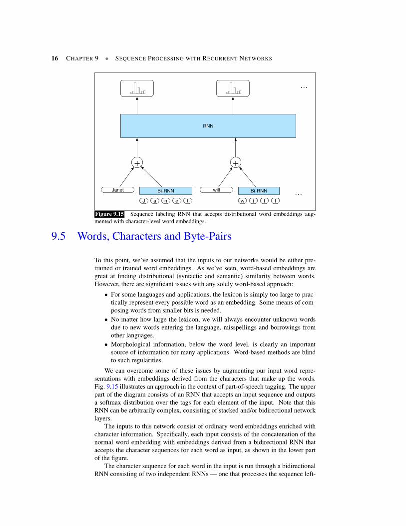
We can overcome some of these issues by augmenting our input word repre-sentations with embeddings derived from the characters that make up the words.Fig. 9.15 illustrates an approach in the context of part-of-speech tagging. The upperpart of the diagram consists of an RNN that accepts an input sequence and outputsa softmax distribution over the tags for each element of the input. Note that thisRNN can be arbitrarily complex, consisting of stacked and/or bidirectional networklayers.
The inputs to this network consist of ordinary word embeddings enriched withcharacter information. Specifically, each input consists of the concatenation of thenormal word embedding with embeddings derived from a bidirectional RNN thataccepts the character sequences for each word as input, as shown in the lower partof the figure.
The character sequence for each word in the input is run through a bidirectionalRNN consisting of two independent RNNs — one that processes the sequence left-
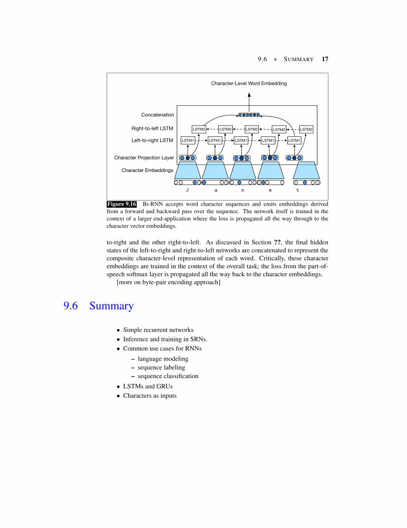
9.6 • SUMMARY 17
J a n e
Character Projection Layer
LSTM1 LSTM1 LSTM1 LSTM1
LSTM2 LSTM2 LSTM2 LSTM2Right-to-left LSTM
Left-to-right LSTM
t
LSTM2
LSTM1
Concatenation
Character-Level Word Embedding
Character Embeddings
Figure 9.16 Bi-RNN accepts word character sequences and emits embeddings derivedfrom a forward and backward pass over the sequence. The network itself is trained in thecontext of a larger end-application where the loss is propagated all the way through to thecharacter vector embeddings.
to-right and the other right-to-left. As discussed in Section ??, the final hiddenstates of the left-to-right and right-to-left networks are concatenated to represent thecomposite character-level representation of each word. Critically, these characterembeddings are trained in the context of the overall task; the loss from the part-of-speech softmax layer is propagated all the way back to the character embeddings.
[more on byte-pair encoding approach]
9.6 Summary
• Simple recurrent networks• Inference and training in SRNs.• Common use cases for RNNs
– language modeling– sequence labeling– sequence classification
• LSTMs and GRUs• Characters as inputs
18 Chapter 9 • Sequence Processing with Recurrent Networks
Elman, J. L. (1990). Finding structure in time. Cognitivescience, 14(2), 179–211.
Ramshaw, L. A. and Marcus, M. P. (1995). Text chunkingusing transformation-based learning. In Proceedings of the3rd Annual Workshop on Very Large Corpora, pp. 82–94.