chapter 14testbanksinstant.eu/samples/solution manual for... · web viewfull file at...

Full file at http://testbanksinstant.eu/ Solution-Manual-for-essentials-of-business-analytics-15th-jeffrey

Chapter 10Nonlinear Optimization Models

Solutions:

1.

a. With $2000 being spent on radio and $1000 being spent on direct mail we can simply substitute those values into the sales function (remembering that the variables are defined as thousands of dollars).

Sales of $36,000 will be realized with this allocation of the media budget.

b. We simply add a budget constraint and nonnegativity constraint to the sales function that is to be maximized.

The solution is R = $2,500 and M = $500 with Sales of $37,000. The spreadsheet model is:

10 - 1


2. a. The optimization model is

10 - 2


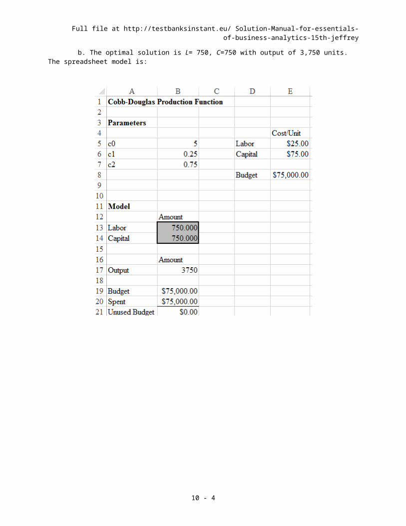
b. The optimal solution is L= 750, C=750 with output of 3,750 units. The spreadsheet model is:

10 - 3


10 - 4


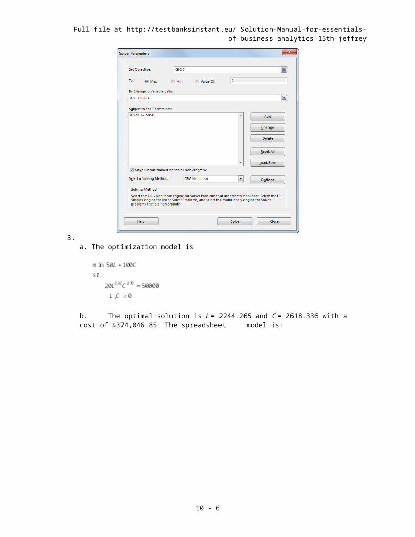
3. a. The optimization model is

b. The optimal solution is L = 2244.265 and C = 2618.336 with a cost of $374,046.85. The spreadsheet model is:

10 - 5


10 - 6


4. Let OT be the number of overtime hours scheduled. Then the optimization model is

The optimal solution is: x1 = 3.667 and x2 = 3.00 with a profit of $887.333. The spreadsheet model is:

10 - 7


10 - 8


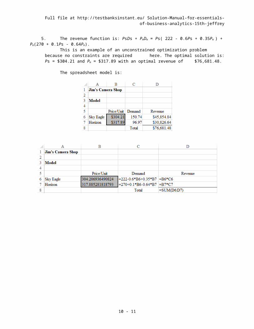
5. The revenue function is: PsDs + PHDH = Ps( 222 - 0.6Ps + 0.35PH ) + PH(270 + 0.1Ps - 0.64PH).This is an example of an unconstrained optimization problem because no constraints are required here. The optimal solution is: Ps = $304.21 and PH = $317.89 with an optimal revenue of $76,681.48.

The spreadsheet model is:

10 - 9


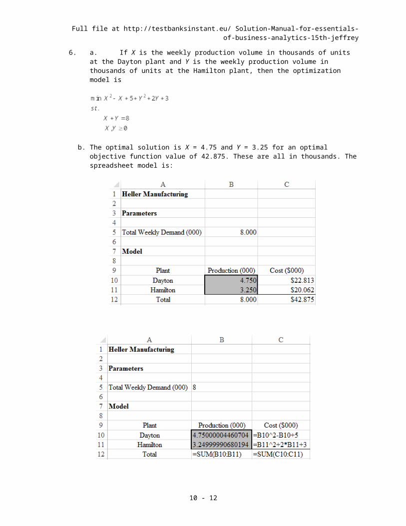
6. a. If X is the weekly production volume in thousands of units at the Dayton plant and Y is the weekly production volume in thousands of units at the Hamilton plant, then the optimization model is

b. The optimal solution is X = 4.75 and Y = 3.25 for an optimal objective function value of 42.875. These are all in thousands. The spreadsheet model is:

10 - 10


10 - 11


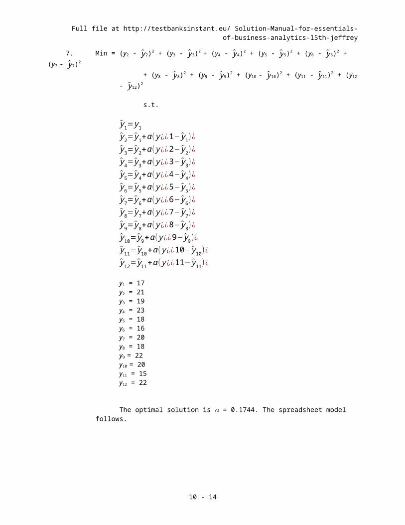
7. Min = (y2 - y2)2 + (y3 - y3)2 + (y4 - y4)2 + (y5 - y5)2 + (y6 - y6)2 + (y7 - y7)2 + (y8 - y8)2 + (y9 - y9)2 + (y10 - y10)2 + (y11 - y11)2 + (y12 - y12)2

s.t.

y1= y1

y2= y1+α ( y¿¿1− y1)¿y3= y2+α ( y¿¿2− y2)¿y4= y3+α ( y¿¿3− y3)¿y5= y 4+α ( y¿¿4− y4)¿y6= y5+α ( y¿¿5− y5)¿y7= y6+α ( y¿¿6− y6)¿y8= y7+α ( y¿¿7− y7)¿y9= y8+α ( y¿¿8− y8)¿y10= y9+α ( y¿¿9− y9)¿y11= y10+α ( y¿¿10− y10)¿y12= y11+α ( y¿¿11− y11)¿

y1 = 17y2 = 21y3 = 19y4 = 23y5 = 18y6 = 16y7 = 20y8 = 18y9 = 22y10 = 20y11 = 15y12 = 22

The optimal solution is = 0.1744. The spreadsheet model follows.

10 - 12


10 - 13


8. The objective is to minimize total production cost. To minimize total production cost, we minimize the production cost at Aynor plus the production cost at Spartanburg subject to the constraint that total production of kitchen chairs is equal to 40. The model is:

The optimal solution to this model is to produce 10 chairs at Aynor for a production cost of $1350 and 30 chairs at Spartanburg for a production cost of $3150. The total cost is $4500. The spreadsheet model follows.

10 - 14


10 - 15


10 - 16


9. The optimal solution is Q1 = 52.223, Q2 = 70.065, Q3 = 37.689 with a total cost of $25,830.

10 - 17


10 - 18


10. Max 1.2712 LN(XA) + 17.414 + 0.3970 LN(XB) + 16.109s.t.

XA + XB ≤ 500XA ≥ 0XB ≥ 0

The optimal solution is XA = 381.009 and XB = 118.006 (these are in thousands of dollars) with a profit of $42.975 million. The spreadsheet model follows.

10 - 19


10 - 20


11. The demand-weighted objective is:

The solution to the un-weighted model is X = 2.23 and Y = 3.349 (from section 10.3)

The solution to the demand-weighted model is: X = 1.909 and Y = 2.721

The solutions are shown in the charts below. The size of the bubble indicates the demand. The demand weighted solution shifts the optimal location towards the Paint station.

10 - 21


12. Let X = the horizontal coordinate of the tower.Y = the vertical coordinate of the tower.

The optimal solution is X = 12, Y = 16, with an objective function value of 16.797.

10 - 22


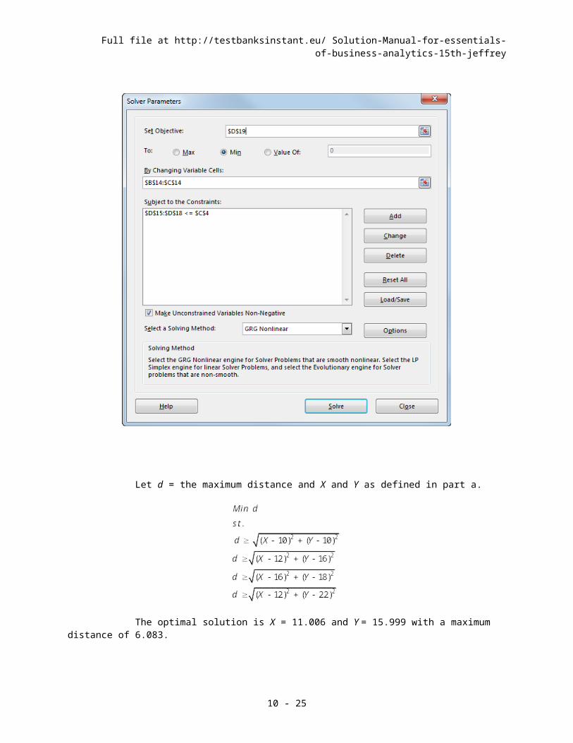
Let d = the maximum distance and X and Y as defined in part a.

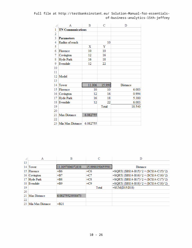
The optimal solution is X = 11.006 and Y = 15.999 with a maximum distance of 6.083.

10 - 23


10 - 24


Note that the decision variable d is located in cell B21 and the objective function is cell B23. This approach is necessary because Excel Solver will not let the objective function and a decision variable be the same cell.

10 - 25


13. Let X = the latitude of the optimal wedding location.Y = the longitude of the optimal wedding location.

The optimal solution is X = 40.204, Y = -75.214, with an objective function value of 67,444.286.

10 - 26


10 - 27


14. Let X = the fraction of the portfolio to invest in AAPLY = the fraction of the portfolio to invest in AMDZ = the fraction of the portfolio to invest in ORCL

10 - 28


10 - 29


10 - 30


15. Let:

= the expected return of the portfolio

= the return of the portfolio in year s

10 - 31


10 - 32


10 - 33


10 - 34


16. Let X = the fraction of the portfolio to invest in Stock 1Y = the fraction of the portfolio to invest in Stock 2Z = the fraction of the portfolio to invest in Stock 3

10 - 35


10 - 36


10 - 37


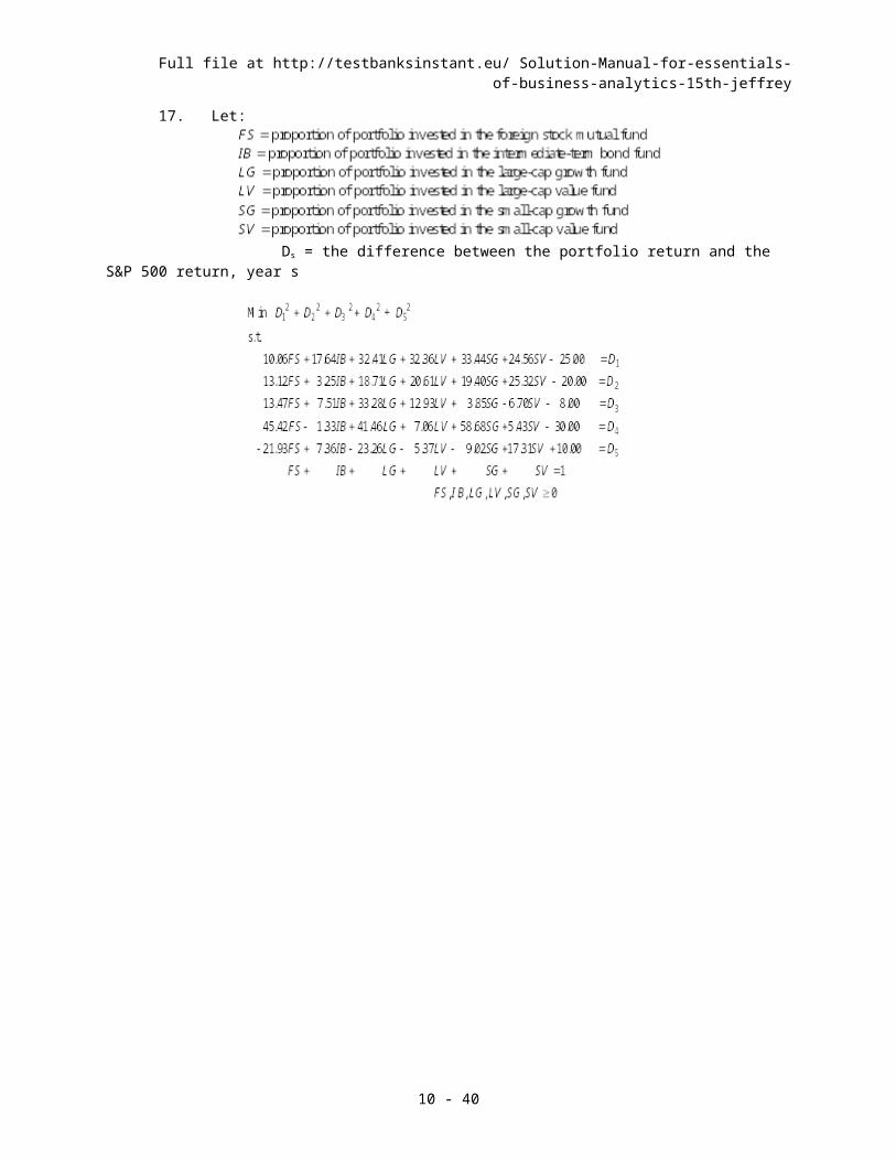
17. Let:

Ds = the difference between the portfolio return and the S&P 500 return, year s

10 - 38


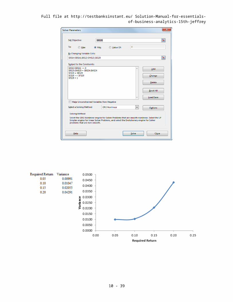
Note from the dialog box that follows, cells B17 through F17 are not designated as decision variables. Rather they are simple calculations in the spreadsheet. These cells correspond

to the deviation variables defined in the algebraic model.

10 - 39


10 - 40


18. Let:

= expected return of the portfolio Rs = the return of the portfolio in year s

ds = the difference between the expected portfolio return and return for year s

10 - 41


10 - 42


10 - 43


10 - 44


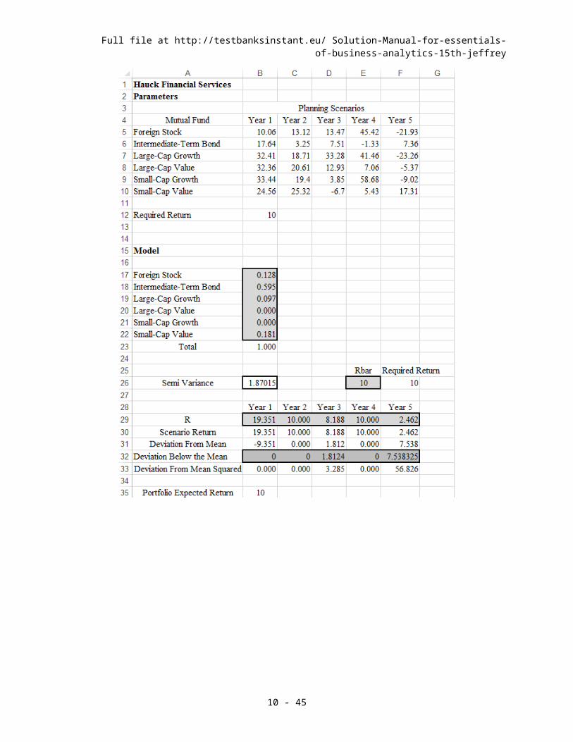
19. The frontier is shown below. As the maximum variance increases the expected return increases but at a decreasing rate. In Figure 10.12, as the required expected return increases, the variance

increases at an increasing rate. These curves are known as the efficient frontier and are really the same curve from two different perspectives. For example, a variance of 40 with an expected return of 11.835 is on both curves.

10 - 45


20. A spreadsheet model follows. Results might vary somewhat form the values in Table 10.4

10 - 46


10 - 47


We used the Multistart option with population size of 100, but not requiring bounds. We used a starting point of m = 149.89, with p = q = 0.

10 - 48

chapter 14testbanksinstant.eu/samples/solution manual for... · web viewfull file at...

Documents