chapter laplace transforms - uncw faculty and staff...

Chapter 5

Laplace Transforms

“We could, of course, use any notation we want; do not laugh at notations; inventthem, they are powerful. In fact, mathematics is, to a large extent, invention ofbetter notations.” - Richard P. Feynman (1918-1988)

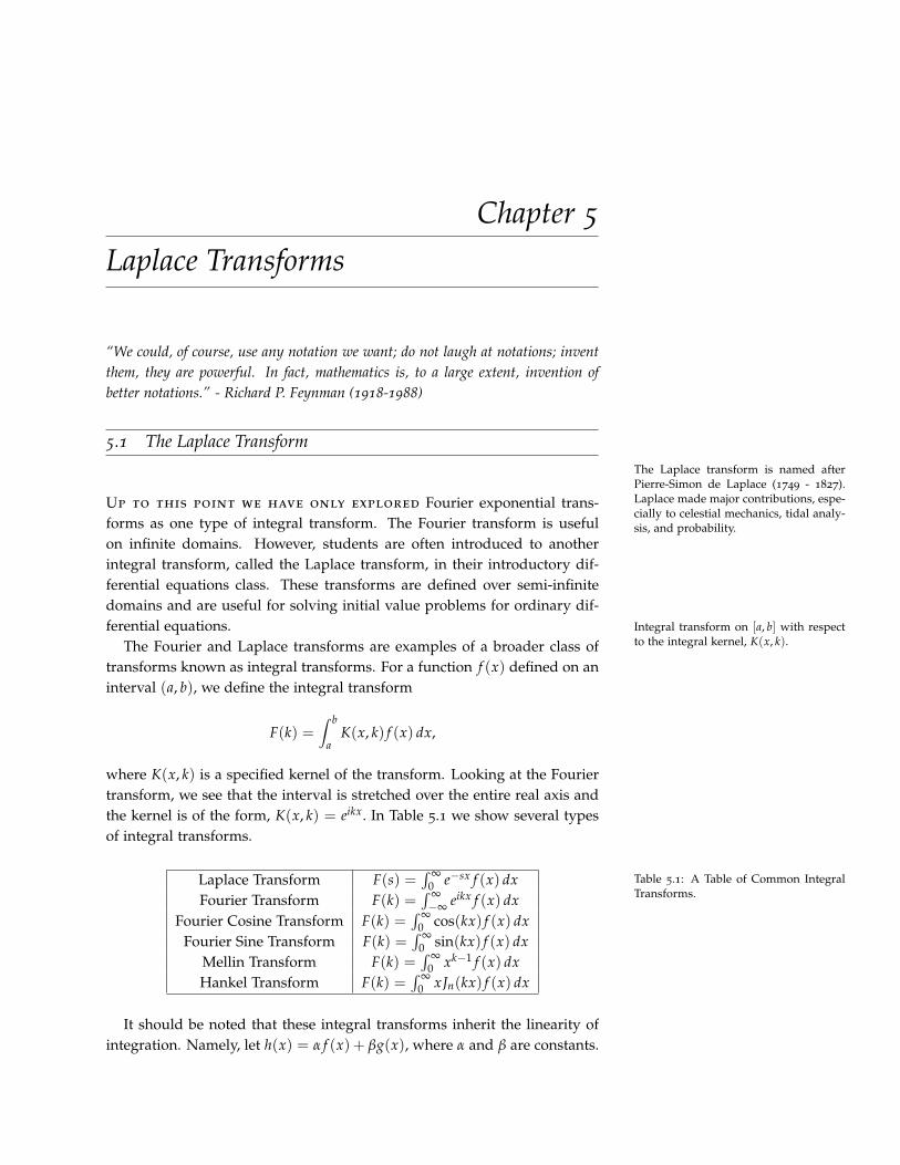
5.1 The Laplace TransformThe Laplace transform is named afterPierre-Simon de Laplace (1749 - 1827).Laplace made major contributions, espe-cially to celestial mechanics, tidal analy-sis, and probability.

Up to this point we have only explored Fourier exponential trans-forms as one type of integral transform. The Fourier transform is usefulon infinite domains. However, students are often introduced to anotherintegral transform, called the Laplace transform, in their introductory dif-ferential equations class. These transforms are defined over semi-infinitedomains and are useful for solving initial value problems for ordinary dif-ferential equations. Integral transform on [a, b] with respect

to the integral kernel, K(x, k).The Fourier and Laplace transforms are examples of a broader class oftransforms known as integral transforms. For a function f (x) defined on aninterval (a, b), we define the integral transform

F(k) =∫ b

aK(x, k) f (x) dx,

where K(x, k) is a specified kernel of the transform. Looking at the Fouriertransform, we see that the interval is stretched over the entire real axis andthe kernel is of the form, K(x, k) = eikx. In Table 5.1 we show several typesof integral transforms.

Laplace Transform F(s) =∫ ∞

0 e−sx f (x) dxFourier Transform F(k) =

∫ ∞−∞ eikx f (x) dx

Fourier Cosine Transform F(k) =∫ ∞

0 cos(kx) f (x) dxFourier Sine Transform F(k) =

∫ ∞0 sin(kx) f (x) dx

Mellin Transform F(k) =∫ ∞

0 xk−1 f (x) dxHankel Transform F(k) =

∫ ∞0 xJn(kx) f (x) dx

Table 5.1: A Table of Common IntegralTransforms.

It should be noted that these integral transforms inherit the linearity ofintegration. Namely, let h(x) = α f (x) + βg(x), where α and β are constants.

178 differential equations

Then,

H(k) =∫ b

aK(x, k)h(x) dx,

=∫ b

aK(x, k)(α f (x) + βg(x)) dx,

= α∫ b

aK(x, k) f (x) dx + β

∫ b

aK(x, k)g(x) dx,

= αF(x) + βG(x). (5.1)

Therefore, we have shown linearity of the integral transforms. We have seenthe linearity property used for Fourier transforms and we will use linearityin the study of Laplace transforms.The Laplace transform of f , F = L[ f ].

We now turn to Laplace transforms. The Laplace transform of a functionf (t) is defined as

F(s) = L[ f ](s) =∫ ∞

0f (t)e−st dt, s > 0. (5.2)

This is an improper integral and one needs

limt→∞

f (t)e−st = 0

to guarantee convergence.Laplace transforms also have proven useful in engineering for solving

circuit problems and doing systems analysis. In Figure 5.1 it is shown thata signal x(t) is provided as input to a linear system, indicated by h(t). Oneis interested in the system output, y(t), which is given by a convolutionof the input and system functions. By considering the transforms of x(t)and h(t), the transform of the output is given as a product of the Laplacetransforms in the s-domain. In order to obtain the output, one needs tocompute a convolution product for Laplace transforms similar to the convo-lution operation we had seen for Fourier transforms earlier in the chapter.Of course, for us to do this in practice, we have to know how to computeLaplace transforms.

Figure 5.1: A schematic depicting theuse of Laplace transforms in systemstheory.

x(t)

LaplaceTransform

X(s)

h(t)

H(s)

y(t) = h(t) ∗ x(t)

Inverse LaplaceTransform

Y(s) = H(s)X(s)

5.2 Properties and Examples of Laplace Transforms

It is typical that one makes use of Laplace transforms by referring toa Table of transform pairs. A sample of such pairs is given in Table 5.2.

laplace transforms 179

Combining some of these simple Laplace transforms with the properties ofthe Laplace transform, as shown in Table 5.3, we can deal with many ap-plications of the Laplace transform. We will first prove a few of the givenLaplace transforms and show how they can be used to obtain new trans-form pairs. In the next section we will show how these transforms can beused to sum infinite series and to solve initial value problems for ordinarydifferential equations.

f (t) F(s) f (t) F(s)

ccs

eat 1s− a

, s > a

tn n!sn+1 , s > 0 tneat n!

(s− a)n+1

sin ωtω

s2 + ω2 eat sin ωt ω(s−a)2+ω2

cos ωts

s2 + ω2 eat cos ωts− a

(s− a)2 + ω2

t sin ωt2ωs

(s2 + ω2)2 t cos ωts2 −ω2

(s2 + ω2)2

sinh ata

s2 − a2 cosh ats

s2 − a2

H(t− a)e−as

s, s > 0 δ(t− a) e−as, a ≥ 0, s > 0

Table 5.2: Table of Selected LaplaceTransform Pairs.

We begin with some simple transforms. These are found by simply usingthe definition of the Laplace transform.

Example 5.1. Show that L[1] = 1s .

For this example, we insert f (t) = 1 into the definition of theLaplace transform:

L[1] =∫ ∞

0e−st dt.

This is an improper integral and the computation is understood byintroducing an upper limit of a and then letting a → ∞. We will notalways write this limit, but it will be understood that this is how onecomputes such improper integrals. Proceeding with the computation,we have

L[1] =∫ ∞

0e−st dt

= lima→∞

∫ a

0e−st dt

= lima→∞

(−1

se−st

)a

0

= lima→∞

(−1

se−sa +

1s

)=

1s

. (5.3)

Thus, we have found that the Laplace transform of 1 is 1s . This result

can be extended to any constant c, using the linearity of the transform,L[c] = cL[1]. Therefore,

L[c] = cs

.


Example 5.2. Show that L[eat] = 1s−a , for s > a.

For this example, we can easily compute the transform. Again, weonly need to compute the integral of an exponential function.

L[eat] =∫ ∞

0eate−st dt

=∫ ∞

0e(a−s)t dt

=

(1

a− se(a−s)t

)∞

0

= limt→∞

1a− s

e(a−s)t − 1a− s

=1

s− a. (5.4)

Note that the last limit was computed as limt→∞ e(a−s)t = 0. Thisis only true if a− s < 0, or s > a. [Actually, a could be complex. Inthis case we would only need s to be greater than the real part of a,s > Re(a).]

Example 5.3. Show that L[cos at] = ss2+a2 and L[sin at] = a

s2+a2 .For these examples, we could again insert the trigonometric func-

tions directly into the transform and integrate. For example,

L[cos at] =∫ ∞

0e−st cos at dt.

Recall how one evaluates integrals involving the product of a trigono-metric function and the exponential function. One integrates by partstwo times and then obtains an integral of the original unknown in-tegral. Rearranging the resulting integral expressions, one arrives atthe desired result. However, there is a much simpler way to computethese transforms.

Recall that eiat = cos at + i sin at. Making use of the linearity of theLaplace transform, we have

L[eiat] = L[cos at] + iL[sin at].

Thus, transforming this complex exponential will simultaneously pro-vide the Laplace transforms for the sine and cosine functions!

The transform is simply computed as

L[eiat] =∫ ∞

0eiate−st dt =

∫ ∞

0e−(s−ia)t dt =

1s− ia

.

Note that we could easily have used the result for the transform of anexponential, which was already proven. In this case, s > Re(ia) = 0.

We now extract the real and imaginary parts of the result using thecomplex conjugate of the denominator:

1s− ia

=1

s− ias + ias + ia

=s + ia

s2 + a2 .


Reading off the real and imaginary parts, we find the sought-aftertransforms,

L[cos at] =s

s2 + a2 ,

L[sin at] =a

s2 + a2 . (5.5)

Example 5.4. Show that L[t] = 1s2 .

For this example we evaluate

L[t] =∫ ∞

0te−st dt.

This integral can be evaluated using the method of integration byparts: ∫ ∞

0te−st dt = −t

1s

e−st∣∣∣∞0+

1s

∫ ∞

0e−st dt

=1s2 . (5.6)

Example 5.5. Show that L[tn] = n!sn+1 for nonnegative integer n.

We have seen the n = 0 and n = 1 cases: L[1] = 1s and L[t] = 1

s2 .We now generalize these results to nonnegative integer powers, n > 1,of t. We consider the integral

L[tn] =∫ ∞

0tne−st dt.

Following the previous example, we again integrate by parts:1 1 This integral can just as easily be doneusing differentiation. We note that(− d

ds

)n ∫ ∞

0e−st dt =

∫ ∞

0tne−st dt.

Since ∫ ∞

0e−st dt =

1s

,∫ ∞

0tne−st dt =

(− d

ds

)n 1s=

n!sn+1 .

∫ ∞

0tne−st dt = −tn 1

se−st

∣∣∣∞0+

ns

∫ ∞

0t−ne−st dt

=ns

∫ ∞

0t−ne−st dt. (5.7)

We could continue to integrate by parts until the final integral iscomputed. However, look at the integral that resulted after one inte-gration by parts. It is just the Laplace transform of tn−1. So, we canwrite the result as

L[tn] =nsL[tn−1].

We compute∫ ∞

0 tne−st dt by turning itinto an initial value problem for a first-order difference equation and findingthe solution using an iterative method.

This is an example of a recursive definition of a sequence. In thiscase, we have a sequence of integrals. Denoting

In = L[tn] =∫ ∞

0tne−st dt

and noting that I0 = L[1] = 1s , we have the following:

In =ns

In−1, I0 =1s

. (5.8)

This is also what is called a difference equation. It is a first-orderdifference equation with an “initial condition,” I0. The next step is tosolve this difference equation.


Finding the solution of this first-order difference equation is easy todo using simple iteration. Note that replacing n with n− 1, we have

In−1 =n− 1

sIn−2.

Repeating the process, we find

In =ns

In−1

=ns

(n− 1

sIn−2

)=

n(n− 1)s2 In−2

=n(n− 1)(n− 2)

s3 In−3. (5.9)

We can repeat this process until we get to I0, which we know. Wehave to carefully count the number of iterations. We do this by iterat-ing k times and then figuring out how many steps will get us to theknown initial value. A list of iterates is easily written out:

In =ns

In−1

=n(n− 1)

s2 In−2

=n(n− 1)(n− 2)

s3 In−3

= . . .

=n(n− 1)(n− 2) . . . (n− k + 1)

sk In−k. (5.10)

Since we know I0 = 1s , we choose to stop at k = n obtaining

In =n(n− 1)(n− 2) . . . (2)(1)

sn I0 =n!

sn+1 .

Therefore, we have shown that L[tn] = n!sn+1 .

Such iterative techniques are useful in obtaining a variety of inte-grals, such as In =

∫ ∞−∞ x2ne−x2

dx.

As a final note, one can extend this result to cases when n is not aninteger. To do this, we use the Gamma function, which was discussed inSection 4.7. Recall that the Gamma function is the generalization of thefactorial function and is defined as

Γ(x) =∫ ∞

0tx−1e−t dt. (5.11)

Note the similarity to the Laplace transform of tx−1 :

L[tx−1] =∫ ∞

0tx−1e−st dt.

For x− 1 an integer and s = 1, we have that

Γ(x) = (x− 1)!.


Thus, the Gamma function can be viewed as a generalization of the factorialand we have shown that

L[tp] =Γ(p + 1)

sp+1

for p > −1.Now we are ready to introduce additional properties of the Laplace trans-

form in Table 5.3. We have already discussed the first property, which is aconsequence of the linearity of integral transforms. We will prove the otherproperties in this and the following sections.

Laplace Transform PropertiesL[a f (t) + bg(t)] = aF(s) + bG(s)

L[t f (t)] = − dds

F(s)

L[

d fdt

]= sF(s)− f (0)

L[

d2 fdt2

]= s2F(s)− s f (0)− f ′(0)

L[eat f (t)] = F(s− a)L[H(t− a) f (t− a)] = e−asF(s)

L[( f ∗ g)(t)] = L[∫ t

0f (t− u)g(u) du] = F(s)G(s)

Table 5.3: Table of selected Laplacetransform properties.

Example 5.6. Show that L[

d fdt

]= sF(s)− f (0).

We have to compute

L[

d fdt

]=∫ ∞

0

d fdt

e−st dt.

We can move the derivative off f by integrating by parts. This is sim-ilar to what we had done when finding the Fourier transform of thederivative of a function. Letting u = e−st and v = f (t), we have

L[

d fdt

]=

∫ ∞

0

d fdt

e−st dt

= f (t)e−st∣∣∣∞0+ s

∫ ∞

0f (t)e−st dt

= − f (0) + sF(s). (5.12)

Here we have assumed that f (t)e−st vanishes for large t.The final result is that

L[

d fdt

]= sF(s)− f (0).

Example 6: Show that L[

d2 fdt2

]= s2F(s)− s f (0)− f ′(0).

We can compute this Laplace transform using two integrations byparts, or we could make use of the last result. Letting g(t) = d f (t)

dt , wehave

L[

d2 fdt2

]= L

[dgdt

]= sG(s)− g(0) = sG(s)− f ′(0).


But,

G(s) = L[

d fdt

]= sF(s)− f (0).

So,

L[

d2 fdt2

]= sG(s)− f ′(0)

= s [sF(s)− f (0)]− f ′(0)

= s2F(s)− s f (0)− f ′(0). (5.13)

We will return to the other properties in Table 5.3 after looking at a fewapplications.

5.3 Solution of ODEs Using Laplace Transforms

One of the typical applications of Laplace transforms is the so-lution of nonhomogeneous linear constant coefficient differential equations.In the following examples we will show how this works.

The general idea is that one transforms the equation for an unknownfunction y(t) into an algebraic equation for its transform, Y(t). Typically,the algebraic equation is easy to solve for Y(s) as a function of s. Then,one transforms back into t-space using Laplace transform tables and theproperties of Laplace transforms. The scheme is shown in Figure 5.2.

Figure 5.2: The scheme for solvingan ordinary differential equation usingLaplace transforms. One transforms theinitial value problem for y(t) and obtainsan algebraic equation for Y(s). Solve forY(s) and the inverse transform gives thesolution to the initial value problem.

L[y] = g

y(t)

F(Y) = G

Y(s)

Laplace Transform

Inverse Laplace Transform

ODEfor y(t)

Algebraic

Equation

Y(s)

Example 5.7. Solve the initial value problem y′ + 3y = e2t, y(0) = 1.The first step is to perform a Laplace transform of the initial value

problem. The transform of the left side of the equation is

L[y′ + 3y] = sY− y(0) + 3Y = (s + 3)Y− 1.

Transforming the right-hand side, we have

L[e2t] =1

s− 2.

Combining these two results, we obtain

(s + 3)Y− 1 =1

s− 2.


The next step is to solve for Y(s) :

Y(s) =1

s + 3+

1(s− 2)(s + 3)

.

Now we need to find the inverse Laplace transform. Namely, weneed to figure out what function has a Laplace transform of the aboveform. We will use the tables of Laplace transform pairs. Later wewill show that there are other methods for carrying out the Laplacetransform inversion.

The inverse transform of the first term is e−3t. However, we have notseen anything that looks like the second form in the table of transformsthat we have compiled, but we can rewrite the second term using apartial fraction decomposition. Let’s recall how to do this.

The goal is to find constants A and B such that

1(s− 2)(s + 3)

=A

s− 2+

Bs + 3

. (5.14)

We picked this form because we know that recombining the two terms This is an example of carrying out a par-tial fraction decomposition.into one term will have the same denominator. We just need to make

sure the numerators agree afterward. So, adding the two terms, wehave

1(s− 2)(s + 3)

=A(s + 3) + B(s− 2)

(s− 2)(s + 3).

Equating numerators,

1 = A(s + 3) + B(s− 2).

There are several ways to proceed at this point.

a. Method 1.

We can rewrite the equation by gathering terms with common powersof s, we have

(A + B)s + 3A− 2B = 1.

The only way that this can be true for all s is that the coefficients of thedifferent powers of s agree on both sides. This leads to two equationsfor A and B:

A + B = 0,

3A− 2B = 1. (5.15)

The first equation gives A = −B, so the second equation becomes−5B = 1. The solution is then A = −B = 1

5 .

b. Method 2.

Since the equation 1(s−2)(s+3) =

As−2 + B

s+3 is true for all s, we can pick

specific values. For s = 2, we find 1 = 5A, or A = 15 . For s = −3, we

find 1 = −5B, or B = − 15 . Thus, we obtain the same result as Method

1, but much quicker.1 2

2

4

6

8

t

y(t)

Figure 5.3: A plot of the solution to Ex-ample 5.7.


c. Method 3.

We could just inspect the original partial fraction problem. Since thenumerator has no s terms, we might guess the form

1(s− 2)(s + 3)

=1

s− 2− 1

s + 3.

But, recombining the terms on the right-hand side, we see that

1s− 2

− 1s + 3

=5

(s− 2)(s + 3).

Since we were off by 5, we divide the partial fractions by 5 to obtain

1(s− 2)(s + 3)

=15

[1

s− 2− 1

s + 3

],

which once again gives the desired form.

Returning to the problem, we have found that

Y(s) =1

s + 3+

15

(1

s− 2− 1

s + 3

).

We can now see that the function with this Laplace transform is givenby

y(t) = L−1[

1s + 3

+15

(1

s− 2− 1

s + 3

)]= e−3t +

15

(e2t − e−3t

)works. Simplifying, we have the solution of the initial value problem

y(t) =15

e2t +45

e−3t.

We can verify that we have solved the initial value problem.

y′ + 3y =25

e2t − 125

e−3t + 3(15

e2t +45

e−3t) = e2t

and y(0) = 15 + 4

5 = 1.

Example 5.8. Solve the initial value problem y′′ + 4y = 0, y(0) = 1,y′(0) = 3.

We can probably solve this without Laplace transforms, but it is asimple exercise. Transforming the equation, we have

0 = s2Y− sy(0)− y′(0) + 4Y

= (s2 + 4)Y− s− 3. (5.16)

Solving for Y, we have

Y(s) =s + 3s2 + 4

.

We now ask if we recognize the transform pair needed. The denom-inator looks like the type needed for the transform of a sine or cosine.


We just need to play with the numerator. Splitting the expression intotwo terms, we have

Y(s) =s

s2 + 4+

3s2 + 4

.

The first term is now recognizable as the transform of cos 2t. Thesecond term is not the transform of sin 2t. It would be if the numeratorwere a 2. This can be corrected by multiplying and dividing by 2:

3s2 + 4

=32

(2

s2 + 4

).

The solution is then found as

y(t) = L−1[

ss2 + 4

+32

(2

s2 + 4

)]= cos 2t +

32

sin 2t.

The reader can verify that this is the solution of the initial value prob-lem and is shown in Figure 5.4. 2 4 6 8

−2

2

t

y(t)

Figure 5.4: A plot of the solution to Ex-ample 5.8.

5.4 Step and Impulse Functions

5.4.1 Heaviside Step Function

Often, the initial value problems that one faces in differentialequations courses can be solved using either the Method of UndeterminedCoefficients or the Method of Variation of Parameters. However, using thelatter can be messy and involves some skill with integration. Many circuitdesigns can be modeled with systems of differential equations using Kir-choff’s Rules. Such systems can get fairly complicated. However, Laplacetransforms can be used to solve such systems, and electrical engineers havelong used such methods in circuit analysis.

In this section we add a couple more transform pairs and transform prop-erties that are useful in accounting for things like turning on a driving force,using periodic functions like a square wave, or introducing impulse forces.

We first recall the Heaviside step function, given by

H(t) =

0, t < 0,1, t > 0.

(5.17)

t

H(t− a)

1

a

Figure 5.5: A shifted Heaviside function,H(t− a).

A more general version of the step function is the horizontally shiftedstep function, H(t− a). This function is shown in Figure 5.5. The Laplacetransform of this function is found for a > 0 as

L[H(t− a)] =∫ ∞

0H(t− a)e−st dt

=∫ ∞

ae−st dt

=e−st

s

∣∣∣∞a=

e−as

s. (5.18)


The Laplace transform has two Shift Theorems involving the multiplica-tion of the function, f (t), or its transform, F(s), by exponentials. The Firstand Second Shift Properties/Theorems are given by

L[eat f (t)] = F(s− a), (5.19)

L[ f (t− a)H(t− a)] = e−asF(s). (5.20)

The Shift Theorems.We prove the First Shift Theorem and leave the other proof as an exercise

for the reader. Namely,

L[eat f (t)] =∫ ∞

0eat f (t)e−st dt

=∫ ∞

0f (t)e−(s−a)t dt = F(s− a). (5.21)

Example 5.9. Compute the Laplace transform of e−at sin ωt.This function arises as the solution of the underdamped harmonic

oscillator. We first note that the exponential multiplies a sine function.The First Shift Theorem tells us that we first need the transform of thesine function. So, for f (t) = sin ωt, we have

F(s) =ω

s2 + ω2 .

Using this transform, we can obtain the solution to this problem as

L[e−at sin ωt] = F(s + a) =ω

(s + a)2 + ω2 .

More interesting examples can be found using piecewise defined func-tions. First we consider the function H(t)− H(t− a). For t < 0, both termsare zero. In the interval [0, a], the function H(t) = 1 and H(t− a) = 0. There-fore, H(t)− H(t− a) = 1 for t ∈ [0, a]. Finally, for t > a, both functions areone and therefore the difference is zero. The graph of H(t) − H(t − a) isshown in Figure 5.6.t

1

0 a

Figure 5.6: The box function, H(t) −H(t− a).

We now consider the piecewise defined function:

g(t) =

f (t), 0 ≤ t ≤ a,0, t < 0, t > a.

This function can be rewritten in terms of step functions. We only need tomultiply f (t) by the above box function,

g(t) = f (t)[H(t)− H(t− a)].

We depict this in Figure 5.7.t

1

0 a

Figure 5.7: Formation of a piecewisefunction, f (t)[H(t)− H(t− a)].

Even more complicated functions can be written in terms of step func-tions. We only need to look at sums of functions of the form f (t)[H(t −a) − H(t − b)] for b > a. This is similar to a box function. It is nonzerobetween a and b and has height f (t).


We show as an example the square wave function in Figure 5.8. It can berepresented as a sum of an infinite number of boxes,

f (t) =∞

∑n=−∞

[H(t− 2na)− H(t− (2n + 1)a)],

for a > 0.

Example 5.10. Find the Laplace Transform of a square wave “turnedon” at t = 0.

t-2a 0 a 2a 4a 6a

Figure 5.8: A square wave, f (t) =

∑∞n=−∞[H(t− 2na)− H(t− (2n + 1)a)].

We let

f (t) =∞

∑n=0

[H(t− 2na)− H(t− (2n + 1)a)], a > 0.

Using the properties of the Heaviside function, we have

L[ f (t)] =∞

∑n=0

[L[H(t− 2na)]−L[H(t− (2n + 1)a)]]

=∞

∑n=0

[e−2nas

s− e−(2n+1)as

s

]

=1− e−as

s

∞

∑n=0

(e−2as

)n

=1− e−as

s

(1

1− e−2as

)=

1− e−as

s(1− e−2as)

=1

s(1 + e−as . (5.22)

Note that the third line in the derivation is a geometric series. Wesummed this series to get the answer in a compact form since e−2as <

1.

5.4.2 Periodic Functions

The previous example provides us with a causal function ( f (t) = 0 fort < 0.) which is periodic with period a. Such periodic functions can beteated in a simpler fashion. We will now show that Laplace transform of periodic functions.

Theorem 5.1. If f (t) is periodic with period T and piecewise continuous on [0, T],then

F(s) =1

1− e−sT

∫ T

0f (t)e−st dt.


Proof.

F(s) =∫ ∞

0f (t)e−st dt

=∫ T

0f (t)e−st dt +

∫ ∞

Tf (t)e−st dt

=∫ T

0f (t)e−st dt +

∫ ∞

Tf (t− T)e−st dt

=∫ T

0f (t)e−st dt + e−sT

∫ ∞

0f (τ)e−sτ dτ

=∫ T

0f (t)e−st dt + e−sT F(s). (5.23)

Solving for F(s), one obtains the desired result.

Example 5.11. Use the periodicity of

f (t) =∞

∑n=0

[H(t− 2na)− H(t− (2n + 1)a)], a > 0

to obtain the Laplace transform.We note that f (t) has period T = 2a. By Theorem 5.1, we have

F(s) =∫ ∞

0f (t)e−st dt

=1

1− e−2as

∫ 2a

0[H(t)− H(t− a)]e−st dt

=1

1− e−2as

[∫ 2a

0e−st dt−

∫ 2a

ae−st dt

]=

11− e−2as

[e−st

−s

∣∣∣2a

0− e−st

−s

∣∣∣2a

a

]=

1s(1− e−2as)

[1− e−2as + e−2as − e−as

]=

1− e−as

s(1− e−2as)

=1

s(1 + e−as). (5.24)

This is the same result that was obtained in the previous example.

5.4.3 Dirac Delta Function

Another useful concept is the impulse function. If we want toapply an impulse function, we can use the Dirac delta function δ(x). This

P. A. M. Dirac (1902-1984) introducedthe δ function in his book, The Princi-ples of Quantum Mechanics, 4th Ed., Ox-ford University Press, 1958, originallypublished in 1930, as part of his orthog-onality statement for a basis of func-tions in a Hilbert space, < ξ ′|ξ ′′ >=cδ(ξ ′ − ξ ′′) in the same way we intro-duced discrete orthogonality using theKronecker delta. Historically, a numberof mathematicians sought to understandthe Diract delta function, culminating inLaurent Schwartz’s (1915-2002) theory ofdistributions in 1945.

is an example of what is known as a generalized function, or a distribution.Dirac had introduced this function in the 1930s in his study of quantum

mechanics as a useful tool. It was later studied in a general theory of dis-tributions and found to be more than a simple tool used by physicists. TheDirac delta function, as any distribution, only makes sense under an in-tegral. Here will will introduce the Dirac delta function through its mainproperties.


The delta function satisfies two main properties:

1. δ(x) = 0 for x 6= 0.

2.∫ ∞−∞ δ(x) dx = 1.

Integration over more general intervals gives

∫ b

aδ(x) dx =

1, 0 ∈ [a, b],0, 0 6∈ [a, b].

(5.25)

Another important property is the sifting property:∫ ∞

−∞δ(x− a) f (x) dx = f (a).

This can be seen by noting that the delta function is zero everywhere exceptat x = a. Therefore, the integrand is zero everywhere and the only contribu-tion from f (x) will be from x = a. So, we can replace f (x) with f (a) underthe integral. Since f (a) is a constant, we have that∫ ∞

−∞δ(x− a) f (x) dx =

∫ ∞

−∞δ(x− a) f (a) dx

= f (a)∫ ∞

−∞δ(x− a) dx = f (a). (5.26)

Example 5.12. Evaluate:∫ ∞−∞ δ(x + 3)x3 dx.

This is a simple use of the sifting property:∫ ∞

−∞δ(x + 3)x3 dx = (−3)3 = −27.

Properties of the Dirac delta function:∫ ∞

−∞δ(x− a) f (x) dx = f (a).

∫ ∞

−∞δ(ax) dx =

1|a|

∫ ∞

−∞δ(y) dy.

Another property results from using a scaled argument, ax. In this case,we show that

δ(ax) = |a|−1δ(x). (5.27)

As usual, this only has meaning under an integral sign. So, we place δ(ax)inside an integral and make a substitution y = ax:

∫ ∞

−∞δ(ax) dx = lim

L→∞

∫ L

−Lδ(ax) dx

= limL→∞

1a

∫ aL

−aLδ(y) dy. (5.28)

If a > 0 then ∫ ∞

−∞δ(ax) dx =

1a

∫ ∞

−∞δ(y) dy.

However, if a < 0 then∫ ∞

−∞δ(ax) dx =

1a

∫ −∞

∞δ(y) dy = −1

a

∫ ∞

−∞δ(y) dy.

The overall difference in a multiplicative minus sign can be absorbed intoone expression by changing the factor 1/a to 1/|a|. Thus,


∫ ∞

−∞δ(ax) dx =

1|a|

∫ ∞

−∞δ(y) dy. (5.29)

Example 5.13. Evaluate∫ ∞−∞(5x + 1)δ(4(x− 2)) dx.

This is a straightforward integration:∫ ∞

−∞(5x + 1)δ(4(x− 2)) dx =

14

∫ ∞

−∞(5x + 1)δ(x− 2) dx =

114

.

The first step is to write δ(4(x − 2)) = 14 δ(x − 2). Then, the final

evaluation is given by

14

∫ ∞

−∞(5x + 1)δ(x− 2) dx =

14(5(2) + 1) =

114

.

The Dirac delta function can be used to represent a unit impulse. Sum-ming over a number of impulses, or point sources, we can describe a generalfunction as shown in Figure 5.9. The sum of impulses located at points ai,i = 1, . . . , n, with strengths f (ai) would be given by

f (x) =n

∑i=1

f (ai)δ(x− ai).

A continuous sum could be written as

f (x) =∫ ∞

−∞f (ξ)δ(x− ξ) dξ.

This is simply an application of the sifting property of the delta function.

f (x)

xa1 a2 a3 a4 a5 a6 a7 a8 a9 a10

Figure 5.9: Plot representing im-pulse forces of height f (ai). The sum∑n

i=1 f (ai)δ(x − ai) describes a generalimpulse function.

We will investigate a case when one would use a single impulse. Whilea mass on a spring is undergoing simple harmonic motion, we hit it foran instant at time t = a. In such a case, we could represent the force as amultiple of δ(t− a).L[δ(t− a)] = e−as.

One would then need the Laplace transform of the delta function to solvethe associated initial value problem. Inserting the delta function into theLaplace transform, we find that for a > 0,

L[δ(t− a)] =∫ ∞

0δ(t− a)e−st dt

=∫ ∞

−∞δ(t− a)e−st dt

= e−as. (5.30)

Example 5.14. Solve the initial value problem y′′ + 4π2y = δ(t − 2),y(0) = y′(0) = 0.

This initial value problem models a spring oscillation with an im-pulse force. Without the forcing term, given by the delta function, thisspring is initially at rest and not stretched. The delta function modelsa unit impulse at t = 2. Of course, we anticipate that at this time thespring will begin to oscillate. We will solve this problem using Laplacetransforms.


First, we transform the differential equation:

s2Y− sy(0)− y′(0) + 4π2Y = e−2s.

Inserting the initial conditions, we have

(s2 + 4π2)Y = e−2s.

Solving for Y(s), we obtain

Y(s) =e−2s

s2 + 4π2 .

We now seek the function for which this is the Laplace transform.The form of this function is an exponential times some Laplace trans-form, F(s). Thus, we need the Second Shift Theorem since the solutionis of the form Y(s) = e−2sF(s) for

F(s) =1

s2 + 4π2 .

We need to find the corresponding f (t) of the Laplace transformpair. The denominator in F(s) suggests a sine or cosine. Since thenumerator is constant, we pick sine. From the tables of transforms, wehave

L[sin 2πt] =2π

s2 + 4π2 .

So, we write

F(s) =1

2π

2π

s2 + 4π2 .

This gives f (t) = (2π)−1 sin 2πt.We now apply the Second Shift Theorem, L[ f (t − a)H(t − a)] =

e−asF(s), or

y(t) = L−1[e−2sF(s)

]= H(t− 2) f (t− 2)

=1

2πH(t− 2) sin 2π(t− 2). (5.31)

5 10 15 20

−0.2

0.2

t

y(t)

Figure 5.10: A plot of the solution to Ex-ample 5.14 in which a spring at rest ex-periences an impulse force at t = 2.

This solution tells us that the mass is at rest until t = 2 and thenbegins to oscillate at its natural frequency. A plot of this solution isshown in Figure 5.10

Example 5.15. Solve the initial value problem

y′′ + y = f (t), y(0) = 0, y′(0) = 0,

where

f (t) =

cos πt, 0 ≤ t ≤ 2,

0, otherwise.

We need the Laplace transform of f (t). This function can be writ-ten in terms of a Heaviside function, f (t) = cos πtH(t − 2). In or-der to apply the Second Shift Theorem, we need a shifted version


of the cosine function. We find the shifted version by noting thatcos π(t− 2) = cos πt. Thus, we have

f (t) = cos πt [H(t)− H(t− 2)]

= cos πt− cos π(t− 2)H(t− 2), t ≥ 0. (5.32)

The Laplace transform of this driving term is

F(s) = (1− e−2s)L[cos πt] = (1− e−2s)s

s2 + π2 .

Now we can proceed to solve the initial value problem. The Laplacetransform of the initial value problem yields

(s2 + 1)Y(s) = (1− e−2s)s

s2 + π2 .

Therefore,

Y(s) = (1− e−2s)s

(s2 + π2)(s2 + 1).

We can retrieve the solution to the initial value problem using theSecond Shift Theorem. The solution is of the form Y(s) = (1 −e−2s)G(s) for

G(s) =s

(s2 + π2)(s2 + 1).

Then, the final solution takes the form

y(t) = g(t)− g(t− 2)H(t− 2).

We only need to find g(t) in order to finish the problem. This iseasily done using the partial fraction decomposition

G(s) =s

(s2 + π2)(s2 + 1)=

1π2 − 1

[s

s2 + 1− s

s2 + π2

].

Then,

g(t) = L−1[

s(s2 + π2)(s2 + 1)

]=

1π2 − 1

(cos t− cos πt) .

The final solution is then given by

y(t) =1

π2 − 1[cos t− cos πt− H(t− 2)(cos(t− 2)− cos πt)] .

A plot of this solution is shown in Figure 5.11.

5 10

−0.4

−0.2

0.2

0.4

t

y(t)

Figure 5.11: A plot of the solution to Ex-ample 5.15 in which a spring at rest ex-periences an piecewise defined force.

5.5 The Convolution Theorem

Finally, we consider the convolution of two functions. Often, we arefaced with having the product of two Laplace transforms that we know andwe seek the inverse transform of the product. For example, let’s say we have


obtained Y(s) = 1(s−1)(s−2) while trying to solve an initial value problem. In

this case, we could find a partial fraction decomposition. But, there areother ways to find the inverse transform, especially if we cannot performa partial fraction decomposition. We could use the Convolution Theoremfor Laplace transforms or we could compute the inverse transform directly.We will look into these methods in the next two sections. We begin withdefining the convolution.

We define the convolution of two functions defined on [0, ∞) much thesame way as we had done for the Fourier transform. The convolution f ∗ gis defined as

( f ∗ g)(t) =∫ t

0f (u)g(t− u) du. (5.33)

Note that the convolution integral has finite limits as opposed to the Fouriertransform case.

The convolution operation has two important properties:The convolution is commutative.

1. The convolution is commutative: f ∗ g = g ∗ f

Proof. The key is to make a substitution y = t− u in the integral. Thismakes f a simple function of the integration variable.

(g ∗ f )(t) =∫ t

0g(u) f (t− u) du

= −∫ 0

tg(t− y) f (y) dy

=∫ t

0f (y)g(t− y) dy

= ( f ∗ g)(t). (5.34)

2. The Convolution Theorem: The Laplace transform of a convolution isthe product of the Laplace transforms of the individual functions:

L[ f ∗ g] = F(s)G(s).The Convolution Theorem for Laplacetransforms.

Proof. Proving this theorem takes a bit more work. We will makesome assumptions that will work in many cases. First, we assumethat the functions are causal, f (t) = 0 and g(t) = 0 for t < 0. Second,we will assume that we can interchange integrals, which needs morerigorous attention than will be provided here. The first assumptionwill allow us to write the finite integral as an infinite integral. Thena change of variables will allow us to split the integral into the prod-uct of two integrals that are recognized as a product of two Laplacetransforms.

Carrying out the computation, we have

L[ f ∗ g] =∫ ∞

0

(∫ t

0f (u)g(t− u) du

)e−st dt


=∫ ∞

0

(∫ ∞

0f (u)g(t− u) du

)e−st dt

=∫ ∞

0f (u)

(∫ ∞

0g(t− u)e−st dt

)du (5.35)

Now, make the substitution τ = t− u. We note that

int∞0 f (u)

(∫ ∞

0g(t− u)e−st dt

)du =

∫ ∞

0f (u)

(∫ ∞

−ug(τ)e−s(τ+u) dτ

)du

However, since g(τ) is a causal function, we have that it vanishes forτ < 0 and we can change the integration interval to [0, ∞). So, after alittle rearranging, we can proceed to the result.

L[ f ∗ g] =∫ ∞

0f (u)

(∫ ∞

0g(τ)e−s(τ+u) dτ

)du

=∫ ∞

0f (u)e−su

(∫ ∞

0g(τ)e−sτ dτ

)du

=

(∫ ∞

0f (u)e−su du

)(∫ ∞

0g(τ)e−sτ dτ

)= F(s)G(s). (5.36)

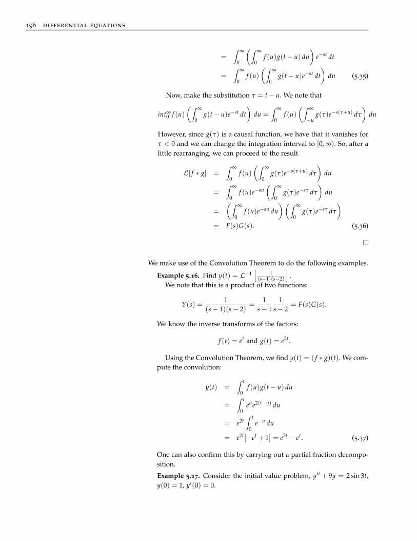
We make use of the Convolution Theorem to do the following examples.

Example 5.16. Find y(t) = L−1[

1(s−1)(s−2)

].

We note that this is a product of two functions:

Y(s) =1

(s− 1)(s− 2)=

1s− 1

1s− 2

= F(s)G(s).

We know the inverse transforms of the factors:

f (t) = et and g(t) = e2t.

Using the Convolution Theorem, we find y(t) = ( f ∗ g)(t). We com-pute the convolution:

y(t) =∫ t

0f (u)g(t− u) du

=∫ t

0eue2(t−u) du

= e2t∫ t

0e−u du

= e2t[−et + 1] = e2t − et. (5.37)

One can also confirm this by carrying out a partial fraction decompo-sition.

Example 5.17. Consider the initial value problem, y′′ + 9y = 2 sin 3t,y(0) = 1, y′(0) = 0.


The Laplace transform of this problem is given by

(s2 + 9)Y− s =6

s2 + 9.

Solving for Y(s), we obtain

Y(s) =6

(s2 + 9)2 +s

s2 + 9.

The inverse Laplace transform of the second term is easily found ascos(3t); however, the first term is more complicated.

We can use the Convolution Theorem to find the Laplace transformof the first term. We note that

6(s2 + 9)2 =

23

3(s2 + 9)

3(s2 + 9)

is a product of two Laplace transforms (up to the constant factor).Thus,

L−1[

6(s2 + 9)2

]=

23( f ∗ g)(t),

where f (t) = g(t) = sin3t. Evaluating this convolution product, wehave

L−1[

6(s2 + 9)2

]=

23( f ∗ g)(t)

=23

∫ t

0sin 3u sin 3(t− u) du

=13

∫ t

0[cos 3(2u− t)− cos 3t] du

=13

[16

sin(6u− 3t)− u cos 3t]t

0

=19

sin 3t− 13

t cos 3t. (5.38)

Combining this with the inverse transform of the second term ofY(s), the solution to the initial value problem is

y(t) = −13

t cos 3t +19

sin 3t + cos 3t.

Note that the amplitude of the solution will grow in time from the firstterm. You can see this in Figure 5.12. This is known as a resonance. 2 4 6 8

−2

2

t

y(t)

Figure 5.12: Plot of the solution to Exam-ple 5.17 showing a resonance.

Example 5.18. Find L−1[ 6(s2+9)2 ] using partial fraction decomposition.

If we look at Table 5.2, we see that the Laplace transform pairs withthe denominator (s2 + ω2)2 are

L[t sin ωt] =2ωs

(s2 + ω2)2 ,

and

L[t cos ωt] =s2 −ω2

(s2 + ω2)2 .


So, we might consider rewriting a partial fraction decomposition as

6(s2 + 9)2 =

A6s(s2 + 9)2 +

B(s2 − 9)(s2 + 9)2 +

Cs + Ds2 + 9

.

Combining the terms on the right over a common denominator, wefind

6 = 6As + B(s2 − 9) + (Cs + D)(s2 + 9).

Collecting like powers of s, we have

Cs3 + (D + B)s2 + 6As + (D− B) = 6.

Therefore, C = 0, A = 0, D + B = 0, and D− B = 23 . Solving the last

two equations, we find D = −B = 13 .

Using these results, we find

6(s2 + 9)2 = −1

3(s2 − 9)(s2 + 9)2 +

13

1s2 + 9

.

This is the result we had obtained in the last example using the Con-volution Theorem.

5.6 Systems of ODEs

Lapace transforms are also useful for solving systems of differentialequations. We will study linear systems of differential equation in Chapter6. For now, we will just look at simple examples of the application of Laplacetransforms.

An example of a system of two differential equations for two unknownfunctions, x(t) and y(t), is given by the pair of coupled differential equations

x′ = 3x + 4y,

y′ = 2x + y. (5.39)

Neither equation can be solved on its own without knowledge of the otherunknown function. This is why they are called couple. We will also needinitial values for the system. We will choose x(0) = 1 and y(0) = 0.

Now, what would happen if we were to take the Laplace transform ofeach equation? We can apply the rules as before. Letting the Laplace trans-forms of x(t) and y(t) be X(t) and Y(t), respectively, we have

sX− 1 = 3X + 4Y,

sY = 2X + Y. (5.40)

We have obtained a system of algebraic equations for X and Y. Usingstandard methods, like Cramer’s Method, we can solve this system of twoequations and two unknowns. First, we rewrite the equations as

(s− 3)X− 4Y = 1,

−2X + (s− 1)Y = 0. (5.41)


Using Cramer’s (determinant) Rule for solving such systems, we have

X =

∣∣∣∣∣ 1 −40 s− 1

∣∣∣∣∣∣∣∣∣∣ s− 3 −4−2 s− 1

∣∣∣∣∣, Y =

∣∣∣∣∣ s− 3 1−2 0

∣∣∣∣∣∣∣∣∣∣ s− 3 −4−2 s− 1

∣∣∣∣∣. (5.42)

Note that the denominator in each solution is a 2× 2 determinant consistingof the coefficients of X and Y in the appropriate order. The numerators arethe same determinant but with the right-hand side of the equation replacingthe respective columns.

Computing the determinants, using∣∣∣∣∣ a bc d

∣∣∣∣∣ = ad− bc,

we have

X =1

(s− 3)(s− 1)− 8, Y =

2(s− 3)(s− 1)− 8

,

or

X =s− 1

s2 − 4s− 5, Y =

2s2 − 4s− 5

.

We now know the Laplace transforms of the solutions, so a simple inverseLaplace transform is in order. The denominators are the same,

s2 − 4s− 5 = (s− 5)(s + 1).

We can apply a partial fraction decomposition to each function to obtain

X =s− 1

(s− 5)(s + 1)

=s− 5 + 4

(s− 5)(s + 1)

=1

s + 1+

4(s− 5)(s + 1)

=1

s + 1+

23

[1

s− 5− 1

s + 1

]=

23

1s− 5

+13

1s + 1

.

Y =2

(s− 5)(s + 1)

=13

[1

s− 5− 1

s + 1

].

So, the solutions to the system of differential equations is given by

x(t) =23

e5t +13

e−t.

y(t) =13(e5t − e−t).


We can verify that x(0) = 1 and y(0) = 0.

x′ =103

e5t − 13

e−t

3x + 4y = (2e5t + e−t) +43(e5t − e−t)

=103

e5t − 13

e−t.

y′ =53

e5t +13

e−t

2x + y = (43

e5t +23

e−t) +13(e5t − e−t)

=53

e5t +13

e−t.

(5.43)

Example 5.19. Determine the current in Figure 5.13 for the followingvalues: i1(0) = i2(0) = i3(0) = 0 and

v(t) =

v0, 0 ≤ t ≤ 3.00, otherwise.

+

−v(t)

L1

L2

R2

A

R1

B

i1 i3

i2

1 2

Figure 5.13: A circuit with two loopscontaining two resistors and two induc-tors in parallel.

The problem can be modeled by a system of differential equations.In Figure 5.13 there are three currents indicated. Kirchoff’s Point(Junction) Rule indicates that i1 = i2 + i3.

In order to apply Kirchoff’s Loop Rule , we need to tally the po-tential drops and rises. For resistors, these come from Ohm’s Law,v = iR, and for inductors, this comes from Faraday’s Law, v = L di

dt .For the left loop (2), we have

L2i′3 = R1i2,

where the prime denotes the time derivative. For the right loop (1),we have

L1i′1 + R1i2 + R2i1 = v(t).

We can use the Point Rule to eliminate one of the currents, i2 = i1− i3,leaving the model as two first order differential equations,

L2i′3 − R1(i1 − i3) = 0

L1i′1 + R1(i1 − i3) + R2i1 = v(t),

or

L2i′3 − R1i1 + R1i3 = 0

L1i′1 + (R1 + R2)i1 − R1i3 = v0(1− H(t− 3)),

where H(t) is the Heaviside function.Taking the Laplace transform, assuming that i1(0) = i2(0) = 0, we

obtain the algebraic system of equations

−R1 I1 + (sL2 + R1)I3 = 0

(sL1 + R1 + R2)I1 − R1 I3 =v0

s

(1− e−3s

).


Here I1(s) and I3(s) are the Laplace transforms of i1(t) and i3(t), re-spectively.

As before, we use Cramer’s Rule to find the solutions.

I1 =

∣∣∣∣∣ 0 sL2 + R1v0s(1− e−3s) −R1

∣∣∣∣∣∣∣∣∣∣ −R1 sL2 + R1

sL1 + R1 + R2 −R1

∣∣∣∣∣,

=−v0(sL2 + R1)

(1− e−3s)

s[R21 − (sL2 + R1)(sL1 + R1 + R2)]

=v0(sL2 + R1)

(1− e−3s)

s[(L1L2)s2 + (R1L1 + L2(R1 + R2))s + R1R2].

I3 =

∣∣∣∣∣ −R1 0sL1 + R1 + R2

v0s(1− e−3s)

∣∣∣∣∣∣∣∣∣∣ −R1 sL2 + R1

sL1 + R1 + R2 −R1

∣∣∣∣∣=

v0R1(1− e−3s)

s[R21 − (sL2 + R1)(sL1 + R1 + R2)]

=−v0R1

(1− e−3s)

s[(L1L2)s2 + (R1L1 + L2(R1 + R2))s + R1R2]. (5.44)

The denominator in these expressions cannot be factored. So, tomake any further progress, one needs specific values for the constants.Let R1 = 2.00Ω, R2 = 18.0Ω, L1 = 48.0 H, L2 = 6.00 H. and v0 = 18V. Then,

I1 =3s + 1

s(2s + 1)(4s + 1)

(1− e−3s

)I3 = − 1

s(2s + 1)(4s + 1)

(1− e−3s

)Using partial fractions on the coefficient of

(1− e−3s) , we find that

3s + 1s(2s + 1)(4s + 1)

=1s− 2

4s + 1− 1

2s + 1,

1s(2s + 1)(4s + 1)

=1s− 8

4s + 1+

22s + 1

.

This gives

I1 =

(1s− 1

21

s + 14− 1

21

s + 12

)(1− e−3s)

I3 =

(−1

s+

2s + 1

4− 1

s + 12

)(1− e−3s)

Taking the inverse Laplace transform, we find the solutions

i1 = 1− 12

e−t4 − 1

2e−

t2 +

(−1 +

12

e−t−3

4 +12

e−t−3

2

)H(t− 3)


=

1− 1

2 e−t4 − 1

2 e−t2 , t ≤ 3,

− 12 (1− e

34 )e−

t4 − 1

2 (1− e32 )e−

t2 , t ≥ 3.

i3 = −1 + 2e−t4 − e−

t2 +

(1− 2e−

t−34 + e−

t−32

)H(t− 3).

=

−1 + 2e−

t4 − e−

t2 , t ≤ 3,

2(1− e34 )e−

t4 − (1− e

32 )e−

t2 , t ≥ 3.

In Figure 5.14 we plot the currents vs time. The taller curve repre-sents i1 and the other curve is −i3. We note that the derived current,i3, is negative, indicating a flow in reverse of the direction shown inFigure 5.13. Not the sudden change in i[1] at t = 3, the time that thevoltage is turned on.Figure 5.14: A plot of the currents vs

time for Example 5.19 with the voltagev(t) = v0(1− H(t− 3)). The taller curverepresents i1 and the other curve is −i3.

One can easily change the time that the voltage is applied. Namely,if

v(t) =

v0, 0 ≤ t ≤ t0

0, otherwise,

then the solutions are given by

i1 = 1− 12

e−t4 − 1

2e−

t2 +

(−1 +

12

e−t−t0

4 +12

e−t−t0

2

)H(t− t0)

i3 = −1 + 2e−t4 − e−

t2 +

(1− 2e−

t−t04 + e−

t−t02

)H(t− t0).

A plot of the currents for t0 = 10 are shown in Figure 5.15.Figure 5.15: A plot of the currents vstime for Example 5.19 for the voltagegiven by v(t) = v0(1− H(t− 10)). Thetaller curve represents i1 and the othercurve is −i3.


Problems

1. Find the Laplace transform of the following functions:

a. f (t) = 9t2 − 7.

b. f (t) = e5t−3.

c. f (t) = cos 7t.

d. f (t) = e4t sin 2t.

e. f (t) = e2t(t + cosh t).

f. f (t) = t2H(t− 1).

g. f (t) =

sin t, t < 4π,

sin t + cos t, t > 4π.

h. f (t) =∫ t

0 (t− u)2 sin u du.

i. f (t) =∫ t

0cosh u du.

j. f (t) = (t + 5)2 + te2t cos 3t and write the answer in the simplestform.

2. Find the inverse Laplace transform of the following functions using theproperties of Laplace transforms and the table of Laplace transform pairs.

a. F(s) =18s3 +

7s

.

b. F(s) =1

s− 5− 2

s2 + 4.

c. F(s) =s + 1s2 + 1

.

d. F(s) =3

s2 + 2s + 2.

e. F(s) =1

(s− 1)2 .

f. F(s) =e−3s

s2 − 1.

g. F(s) =1

s2 + 4s− 5.

h. F(s) =s + 3

s2 + 8s + 17.

3. Compute the convolution ( f ∗ g)(t) (in the Laplace transform sense) andits corresponding Laplace transform L[ f ∗ g] for the following functions:

a. f (t) = t2, g(t) = t3.

b. f (t) = t2, g(t) = cos 2t.

c. f (t) = 3t2 − 2t + 1, g(t) = e−3t.

d. f (t) = δ(t− π

4)

, g(t) = sin 5t.


4. For the following problems, draw the given function and find the Laplacetransform in closed form.

a. f (t) = 1 +∞

∑n=1

(−1)n H(t− n).

b. f (t) =∞

∑n=0

[H(t− 2n + 1)− H(t− 2n)].

c.

f (t) =∞

∑n=0

(t− 2n)[H(t− 2n)− H(t− 2n− 1)]

+∞

∑n=0

(2n + 2− t)[H(t− 2n− 1)− H(t− 2n− 2)].

5. The period, T, and the function defined on its first period are given.Sketch several periods of these periodic functions. Make use of the period-icity to find the Laplace transform of each function.

a. f (t) = sin t, T = 2π.

b. f (t) = t, T = 1.

c. f (t) =

t, 0 ≤ t ≤ 1,

2− t, 1 ≤ t ≤ 2,T = 2.

d. f (t) = t[H(t)− H(t− 1)], T = 2.

e. f (t) = sin t[H(t)− H(t− π)], T = π.

6. Use the Convolution Theorem to compute the inverse transform of thefollowing:

a. F(s) =2

s2(s2 + 1).

b. F(s) =e−3s

s2 .

c. F(s) =1

s(s2 + 2s + 5).

7. Find the inverse Laplace transform in two different ways: (i) Use tables.(ii) Use the Convolution Theorem.

a. F(s) =1

s3(s + 4)2 .

b. F(s) =1

s2 − 4s− 5.

c. F(s) =s + 3

s2 + 8s + 17.

d. F(s) =s + 1

(s− 2)2(s + 4).

e. F(s) =s2 + 8s− 3

(s2 + 2s + 1)(s2 + 1).


8. Use Laplace transforms to solve the following initial value problems.Where possible, describe the solution behavior in terms of oscillation anddecay.

a. y′′ − 5y′ + 6y = 0, y(0) = 2, y′(0) = 0.

b. y′′ − y = te2t, y(0) = 0, y′(0) = 1.

c. y′′ + 4y = δ(t− 1), y(0) = 3, y′(0) = 0.

d. y′′ + 6y′ + 18y = 2H(π − t), y(0) = 0, y′(0) = 0.

9. A linear Volterra integral equation, introduced by Vito Volterra (1860-1940), is of the form

y(t) = f (t) +∫ t

0K(t− τ)y(τ) dτ,

where y(t) is an unknown function and f (t) and the “kernel,” K(t), aregiven functions. The integral is in the form of a convolution integral andsuch equations can be solved using Laplace transforms. Solve the followingVolterra integral equations.

a. y(t) = e−t +∫ t

0 cos(t− τ)y(τ) dτ.

b. y(t) = t−∫ t

0 (t− τ)y(τ) dτ.

c. y(t) = t + 2∫ t

0 et−τy(τ) dτ.

d. sin t =∫ t

0 et−τy(τ) dτ. Note: This is a Volterra integral equation ofthe first kind.

10. Use Laplace transforms to convert the following system of differentialequations into an algebraic system and find the solution of the differentialequations.

x′′ = 3x− 6y, x(0) = 1, x′(0) = 0,

y′′ = x + y, y(0) = 0, y′(0) = 0.

11. Use Laplace transforms to convert the following nonhomogeneous sys-tems of differential equations into an algebraic system and find the solutionsof the differential equations.

a.

x′ = 2x + 3y + 2 sin 2t, x(0) = 1,

y′ = −3x + 2y, y(0) = 0.

b.

x′ = −4x− y + e−t, x(0) = 2,

y′ = x− 2y + 2e−3t, y(0) = −1.

c.

x′ = x− y + 2 cos t, x(0) = 3,

y′ = x + y− 3 sin t, y(0) = 2.


12. Redo Example 5.19 using the values R1 = 1.00Ω, R2 = 1.40Ω, L1 = 0.80H, L2 = 1.00 H. and v0 = 100 V in v(t) = v0(1−H(t− t0)). Plot the currentsas a function of time for several values of t0.

chapter laplace transforms - uncw faculty and staff...

Documents