chapter 7civilwares.free.fr/geotechnical engineering - principles and... · 212 chapter 7 pressure...

CHAPTER 7COMPRESSIBILITY AND CONSOLIDATION

7.1 INTRODUCTIONStructures are built on soils. They transfer loads to the subsoil through the foundations. The effectof the loads is felt by the soil normally up to a depth of about two to three times the width of thefoundation. The soil within this depth gets compressed due to the imposed stresses. Thecompression of the soil mass leads to the decrease in the volume of the mass which results in thesettlement of the structure.

The displacements that develop at any given boundary of the soil mass can be determined ona rational basis by summing up the displacements of small elements of the mass resulting from thestrains produced by a change in the stress system. The compression of the soil mass due to theimposed stresses may be almost immediate or time dependent according to the permeabilitycharacteristics of the soil. Cohesionless soils which are highly permeable are compressed in arelatively short period of time as compared to cohesive soils which are less permeable. Thecompressibility characteristics of a soil mass might be due to any or a combination of the followingfactors:

1. Compression of the solid matter.2. Compression of water and air within the voids.3. Escape of water and air from the voids.

It is quite reasonable and rational to assume that the solid matter and the pore water arerelatively incompressible under the loads usually encountered in soil masses. The change in volumeof a mass under imposed stresses must be due to the escape of water if the soil is saturated. But if thesoil is partially saturated, the change in volume of the mass is partly due to the compression andescape of air from the voids and partly due to the dissolution of air in the pore water.

The compressibility of a soil mass is mostly dependent on the rigidity of the soil skeleton.The rigidity, in turn, is dependent on the structural arrangement of particles and, in fine grained

207

208 Chapter 7

soils, on the degree to which adjacent particles are bonded together. Soils which possess ahoneycombed structure possess high porosity and as such are more compressible. A soil composedpredominantly of flat grains is more compressible than one containing mostly spherical grains. Asoil in an undisturbed state is less compressible than the same soil in a remolded state.

Soils are neither truly elastic nor plastic. When a soil mass is under compression, the volumechange is predominantly due to the slipping of grains one relative to another . The grains do notspring back to their original positions upon removal of the stress. However, a small elastic reboundunder low pressures could be attributed to the elastic compression of the adsorbed watersurrounding the grains.

Soil engineering problems are of two types. The first type includes all cases wherein there isno possibility of the stress being sufficiently large to exceed the shear strength of the soil, butwherein the strains lead to what may be a serious magnitude of displacement of individual grainsleading to settlements within the soil mass. Chapter 7 deals with this type of problem. The secondtype includes cases in which there is danger of shearing stresses exceeding the shear strength of thesoil. Problems of this type are called Stability Problems which are dealt with under the chapters ofearth pressure, stability of slopes, and foundations.

Soil in nature may be found in any of the following states

1. Dry state.

2. Partially saturated state.

3. Saturated state.

Settlements of structures built on granular soils are generally considered only under twostates, that is, either dry or saturated. The stress-strain characteristics of dry sand, depend primarilyon the relative density of the sand, and to a much smaller degree on the shape and size of grains.Saturation does not alter the relationship significantly provided the water content of the sand canchange freely. However, in very fine-grained or silty sands the water content may remain almostunchanged during a rapid change in stress. Under this condition, the compression is time-dependent. Suitable hypotheses relating displacement and stress changes in granular soils have notyet been formulated. However, the settlements may be determined by semi-empirical methods(Terzaghi, Peck and Mesri, 1996).

In the case of cohesive soils, the dry state of the soils is not considered as this state is only ofa temporary nature. When the soil becomes saturated during the rainy season, the soil becomesmore compressible under the same imposed load. Settlement characteristics of cohesive soils are,therefore, considered only under completely saturated conditions. It is quite possible that there aresituations where the cohesive soils may remain partially saturated due to the confinement of airbubbles, gases etc. Current knowledge on the behavior of partially saturated cohesive soils underexternal loads is not sufficient to evolve a workable theory to estimate settlements of structures builton such soils.

7.2 CONSOLIDATIONWhen a saturated clay-water system is subjected to an external pressure, the pressure applied isinitially taken by the water in the pores resulting thereby in an excess pore water pressure. Ifdrainage is permitted, the resulting hydraulic gradients initiate a flow of water out of the clay massand the mass begins to compress. A portion of the applied stress is transferred to the soil skeleton,which in turn causes a reduction in the excess pore pressure. This process, involving a gradualcompression occurring simultaneously with a flow of water out of the mass and with a gradualtransfer of the applied pressure from the pore water to the mineral skeleton is called consolidation.The process opposite to consolidation is called swelling, which involves an increase in the watercontent due to an increase in the volume of the voids.

Compressibility and Consolidation 209

Consolidation may be due to one or more of the following factors:

1. External static loads from structures.2. Self-weight of the soil such as recently placed fills.3. Lowering of the ground water table.4. Desiccation.

The total compression of a saturated clay strata under excess effective pressure may beconsidered as the sum of

1. Immediate compression,2. Primary consolidation, and3. Secondary compression.

The portion of the settlement of a structure which occurs more or less simultaneously with theapplied loads is referred to as the initial or immediate settlement. This settlement is due to theimmediate compression of the soil layer under undrained condition and is calculated by assumingthe soil mass to behave as an elastic soil.

If the rate of compression of the soil layer is controlled solely by the resistance of the flow ofwater under the induced hydraulic gradients, the process is referred to as primary consolidation.The portion of the settlement that is due to the primary consolidation is called primaryconsolidation settlement or compression. At the present time the only theory of practical value forestimating time-dependent settlement due to volume changes, that is under primary consolidationis the one-dimensional theory.

The third part of the settlement is due to secondary consolidation or compression of the claylayer. This compression is supposed to start after the primary consolidation ceases, that is after theexcess pore water pressure approaches zero. It is often assumed that secondary compressionproceeds linearly with the logarithm of time. However, a satisfactory treatment of this phenomenonhas not been formulated for computing settlement under this category.

The Process of ConsolidationThe process of consolidation of a clay-soil-water system may be explained with the help of amechanical model as described by Terzaghi and Frohlich (1936).

The model consists of a cylinder with a frictionless piston as shown in Fig. 7.1. The piston issupported on one or more helical metallic springs. The space underneath the piston is completelyfilled with water. The springs represent the mineral skeleton in the actual soil mass and the waterbelow the piston is the pore water under saturated conditions in the soil mass. When a load of p isplaced on the piston, this stress is fully transferred to the water (as water is assumed to beincompressible) and the water pressure increases. The pressure in the water is

u = p

This is analogous to pore water pressure, u, that would be developed in a clay-water systemunder external pressures. If the whole model is leakproof without any holes in the piston, there is nochance for the water to escape. Such a condition represents a highly impermeable clay-water systemin which there is a very high resistance for the flow of water. It has been found in the case of compactplastic clays that the minimum initial gradient required to cause flow may be as high as 20 to 30.

If a few holes are made in the piston, the water will immediately escape through the holes.With the escape of water through the holes a part of the load carried by the water is transferred tothe springs. This process of transference of load from water to spring goes on until the flow stops

210 Chapter 7

Piston

Spring

Pore water

Figure 7.1 Mechanical model to explain the process of consolidation

when all the load will be carried by the spring and none by the water. The time required to attain thiscondition depends upon the number and size of the holes made in the piston. A few small holesrepresents a clay soil with poor drainage characteristics.

When the spring-water system attains equilibrium condition under the imposed load, thesettlement of the piston is analogous to the compression of the clay-water system under externalpressures.

One-Dimensional Consolidation

In many instances the settlement of a structure is due to the presence of one or more layers of softclay located between layers of sand or stiffer clay as shown in Fig. 7.2A. The adhesion between thesoft and stiff layers almost completely prevents the lateral movement of the soft layers. The theorythat was developed by Terzaghi (1925) on the basis of this assumption is called theone-dimensional consolidation theory. In the laboratory this condition is simulated most closely bythe confined compression or consolidation test.

The process of consolidation as explained with reference to a mechanical model may now beapplied to a saturated clay layer in the field. If the clay strata shown in Fig 7.2 B(a) is subjected to anexcess pressure Ap due to a uniformly distributed load/? on the surface, the clay layer is compressed over

Sand

Sand

Drainagefaces

Figure 7.2A Clay layer sandwiched between sand layers


Drainageboundary

Ap = 55 kPa

Impermeableboundary

10 20 30 40 50Excess porewater pressure (kPa) (a)

Properties of clay:wn = 56-61%, w, = 46%w =24%,pc/p0=l3l

Clay from Berthier-Ville, Canada

3 4 5 6 7Axial compression (mm) (b)

Figure 7.2B (a) Observed distribution of excess pore water pressure duringconsolidation of a soft clay layer; (b) observed distribution of vertical compression

during consolidation of a soft clay layer (after Mesri and Choi, 1985, Mesri andFeng, 1986)

time and excess pore water drains out of it to the sandy layer. This constitutes the process ofconsolidation. At the instant of application of the excess load Ap, the load is carried entirely by water inthe voids of the soil. As time goes on the excess pore water pressure decreases, and the effective vertical

212 Chapter 7

pressure in the layer correspondingly increases. At any point within the consolidating layer, the value uof the excess pore water pressure at a given time may be determined from

u = M. -

where, u = excess pore water pressure at depth z at any time t

u{ = initial total pore water pressure at time t = 0Ap, = effective pressure transferred to the soil grains at depth i and time t

At the end of primary consolidation, the excess pore water pressure u becomes equal to zero.This happens when u = 0 at all depths.

The time taken for full consolidation depends upon the drainage conditions, the thickness of theclay strata, the excess load at the top of the clay strata etc. Fig. 7.2B (a) gives a typical example of anobserved distribution of excess pore water pressure during the consolidation of a soft clay layer 50 cmthick resting on an impermeable stratum with drainage at the top. Figure 7.2B(b) shows thecompression of the strata with the dissipation of pore water pressure. It is clear from the figure that thetime taken for the dissipation of pore water pressure may be quite long, say a year or more.

7.3 CONSOLIDOMETERThe compressibility of a saturated, clay-water system is determined by means of the apparatusshown diagrammatically in Fig. 7.3(a). This apparatus is also known as an oedometer. Figure 7.3(b)shows a table top consolidation apparatus.

The consolidation test is usually performed at room temperature, in floating or fixed rings ofdiameter from 5 to 1 1 cm and from 2 to 4 cm in height. Fig. 7.3(a) is a fixed ring type. In a floatingring type, the ring is free to move in the vertical direction.

Extensometer

Water reservoir

(a)

Figure 7.3 (a) A schematic diagram of a consolidometer


Figure 7.3 (b) Table top consolidation apparatus (Courtesy: Soiltest, USA)

The soil sample is contained in the brass ring between two porous stones about 1.25 cm thick. Bymeans of the porous stones water has free access to and from both surfaces of the specimen. Thecompressive load is applied to the specimen through a piston, either by means of a hanger and deadweights or by a system of levers. The compression is measured on a dial gauge.

At the bottom of the soil sample the water expelled from the soil flows through the filter stoneinto the water container. At the top, a well-jacket filled with water is placed around the stone inorder to prevent excessive evaporation from the sample during the test. Water from the sample alsoflows into the jacket through the upper filter stone. The soil sample is kept submerged in a saturatedcondition during the test.

7.4 THE STANDARD ONE-DIMENSIONAL CONSOLIDATION TESTThe main purpose of the consolidation test on soil samples is to obtain the necessary information aboutthe compressibility properties of a saturated soil for use in determining the magnitude and rate ofsettlement of structures. The following test procedure is applied to any type of soil in the standardconsolidation test.

Loads are applied in steps in such a way that the successive load intensity, p, is twice thepreceding one. The load intensities commonly used being 1/4, 1/2,1, 2,4, 8, and 16 tons/ft2 (25, 50,100,200,400, 800 and 1600 kN/m2). Each load is allowed to stand until compression has practicallyceased (no longer than 24 hours). The dial readings are taken at elapsed times of 1/4, 1/2, 1,2,4, 8,15, 30, 60, 120, 240, 480 and 1440 minutes from the time the new increment of load is put on thesample (or at elpased times as per requirements). Sandy samples are compressed in a relatively shorttime as compared to clay samples and the use of one day duration is common for the latter.

After the greatest load required for the test has been applied to the soil sample, the load isremoved in decrements to provide data for plotting the expansion curve of the soil in order to learn

214 Chapter 7

its elastic properties and magnitudes of plastic or permanent deformations. The following datashould also be obtained:

1. Moisture content and weight of the soil sample before the commencement of the test.

2. Moisture content and weight of the sample after completion of the test.

3. The specific gravity of the solids.

4. The temperature of the room where the test is conducted.

7.5 PRESSURE-VOID RATIO CURVESThe pressure-void ratio curve can be obtained if the void ratio of the sample at the end of eachincrement of load is determined. Accurate determinations of void ratio are essential and may becomputed from the following data:

1. The cross-sectional area of the sample A, which is the same as that of the brass ring.

2. The specific gravity, G^, of the solids.

3. The dry weight, Ws, of the soil sample.

4. The sample thickness, h, at any stage of the test.

Let Vs =• volume of the solids in the samplewhere

w

where yw - unit weight of waterWe can also write

Vs=hsA or hs=^

where, hs = thickness of solid matter.

If e is the void ratio of the sample, then

Ah -Ah, h- h.e =

Ah.. h.. (7.1)

In Eq. (7.1) hs is a constant and only h is a variable which decreases with increment load. Ifthe thickness h of the sample is known at any stage of the test, the void ratio at all the stages of thetest may be determined.

The equilibrium void ratio at the end of any load increment may be determined by the changeof void ratio method as follows:

Change of Void-Ratio Method

In one-dimensional compression the change in height A/i per unit of original height h equals thechange in volume A V per unit of original volume V.

(7.2)h V

V may now be expressed in terms of void ratio e.


; I

V"\>

(a) Initial condition (b) Compressed condition

Figure 7.4 Change of void ratio

We may write (Fig. 7.4),

V

Therefore,

A/i _~h~

or

V-VV

e-eV l+e l + e

l + e

h(7.3)

wherein, t±e = change in void ratio under a load, h = initial height of sample, e = initial void ratio ofsample, e' - void ratio after compression under a load, A/i = compression of sample under the loadwhich may be obtained from dial gauge readings.

Typical pressure-void ratio curves for an undisturbed clay sample are shown in Fig. 7.5,plotted both on arithmetic and on semilog scales. The curve on the log scale indicates clearly twobranches, a fairly horizontal initial portion and a nearly straight inclined portion. The coordinatesof point A in the figure represent the void ratio eQ and effective overburden pressure pQ

corresponding to a state of the clay in the field as shown in the inset of the figure. When a sample isextracted by means of the best of techniques, the water content of the clay does not changesignificantly. Hence, the void ratio eQ at the start of the test is practically identical with that of theclay in the ground. When the pressure on the sample in the consolidometer reaches p0, the e-log pcurve should pass through the point A unless the test conditions differ in some manner from those inthe field. In reality the curve always passes below point A, because even the best sample is at leastslightly disturbed.

The curve that passes through point A is generally termed as afield curve or virgin curve. Insettlement calculations, the field curve is to be used.

216 Chapter 7

Virgincurve

A)

Figure 7.5 Pressure-void ratio curves

Pressure-Void Ratio Curves for Sand

Normally, no consolidation tests are conducted on samples of sand as the compression of sandunder external load is almost instantaneous as can be seen in Fig. 7.6(a) which gives a typical curveshowing the time versus the compression caused by an increment of load.

In this sample more than 90 per cent of the compression has taken place within a period ofless than 2 minutes. The time lag is largely of a frictional nature. The compression is about the samewhether the sand is dry or saturated. The shape of typical e-p curves for loose and dense sands areshown in Fig. 7.6(b). The amount of compression even under a high load intensity is not significantas can be seen from the curves.

Pressure-Void Ratio Curves for Clays

The compressibility characteristics of clays depend on many factors.The most important factors are

1. Whether the clay is normally consolidated or overconsolidated2. Whether the clay is sensitive or insensitive.

% c

onso

lidat

ion

O

OO

ON

-fc'

KJ

O

O

O

O

O

C

\\V

V 1

) 1 2 3 4 5Time in min

l .U

0.9

•2 0.8£

*o'| 0.7

0.6

0.5£

\

^

Rebou

^

S~\

\r\nd cun

Comp

<^•/e

Dense/

ression

— ̂™

sand

curve

j sand

^=^

) 2 4 6 8 1(

(a)

Pressure in kg/cm^

(b)

Figure 7.6 Pressure-void ratio curves for sand


Normally Consolidated and Overconsolidated ClaysA clay is said to be normally consolidated if the present effective overburden pressure pQ is themaximum pressure to which the layer has ever been subjected at any time in its history, whereas aclay layer is said to be overconsolidated if the layer was subjected at one time in its history to agreater effective overburden pressure, /?c, than the present pressure, pQ. The ratio pc I pQ is called theoverconsolidation ratio (OCR).

Overconsolidation of a clay stratum may have been caused due to some of the followingfactors

1. Weight of an overburden of soil which has eroded2. Weight of a continental ice sheet that melted3. Desiccation of layers close to the surface.

Experience indicates that the natural moisture content, wn, is commonly close to the liquidlimit, vv;, for normally consolidated clay soil whereas for the overconsolidated clay, wn is close toplastic limit w .

Fig. 7.7 illustrates schematically the difference between a normally consolidated clay stratasuch as B on the left side of Section CC and the overconsolidated portion of the same layer B on theright side of section CC. Layer A is overconsolidated due to desiccation.

All of the strata located above bed rock were deposited in a lake at a time when the water levelwas located above the level of the present high ground when parts of the strata were removed byerosion, the water content in the clay stratum B on the right hand side of section CC increasedslightly, whereas that of the left side of section CC decreased considerably because of the loweringof the water table level from position DQDQ to DD. Nevertheless, with respect to the presentoverburden, the clay stratum B on the right hand side of section CC is overconsolidated clay, andthat on the left hand side is normally consolidated clay.

While the water table descended from its original to its final position below the floor of theeroded valley, the sand strata above and below the clay layer A became drained. As a consequence,layer A gradually dried out due to exposure to outside heat. Layer A is therefore said to beoverconsolidated by desiccation.

Overconsolidated bydesiccation

DO

C Original water table

Original ground surface

StructurePresent ground

surface

JNormally consolidated clay

• . ; ̂ — Overconsolidated clay/ _ • • : '.

Figure 7.7 Diagram illustrating the geological process leading to overconsolidationof clays (After Terzaghi and Peck, 1967)

218 Chapter 7

7.6 DETERMINATION OF PRECONSOLIDATION PRESSURESeveral methods have been proposed for determining the value of the maximum consolidationpressure. They fall under the following categories. They are

1. Field method,2. Graphical procedure based on consolidation test results.

Field Method

The field method is based on geological evidence. The geology and physiography of the site mayhelp to locate the original ground level. The overburden pressure in the clay structure with respectto the original ground level may be taken as the preconsolidation pressure pc. Usually thegeological estimate of the maximum consolidation pressure is very uncertain. In such instances, theonly remaining procedure for obtaining an approximate value of pc is to make an estimate based onthe results of laboratory tests or on some relationships established between pc and other soilparameters.

Graphical Procedure

There are a few graphical methods for determining the preconsolidation pressure based onlaboratory test data. No suitable criteria exists for appraising the relative merits of the variousmethods.

The earliest and the most widely used method was the one proposed by Casagrande (1936).The method involves locating the point of maximum curvature, 5, on the laboratory e-log p curveof an undisturbed sample as shown in Fig. 7.8. From B, a tangent is drawn to the curve and ahorizontal line is also constructed. The angle between these two lines is then bisected. The abscissaof the point of intersection of this bisector with the upward extension of the inclined straight partcorresponds to the preconsolidation pressure/^,.

Tangent at B

e-log p curve

log p Pc

Figure 7.8 Method of determining p by Casagrande method


7.7 e-log p FIELD CURVES FOR NORMALLY CONSOLIDATED ANDOVERCONSOLIDATED CLAYS OF LOW TO MEDIUM SENSITIVITYIt has been explained earlier with reference to Fig. 7.5, that the laboratory e-log p curve of anundisturbed sample does not pass through point A and always passes below the point. It has beenfound from investigation that the inclined straight portion of e-log p curves of undisturbed orremolded samples of clay soil intersect at one point at a low void ratio and corresponds to 0.4eQ

shown as point C in Fig. 7.9 (Schmertmann, 1955). It is logical to assume the field curve labelled asKf should also pass through this point. The field curve can be drawn from point A, havingcoordinates (eQ, /?0), which corresponds to the in-situ condition of the soil. The straight line AC inFig. 7.9(a) gives the field curve AT,for normally consolidated clay soil of low sensitivity.

The field curve for overconsolidated clay soil consists of two straight lines, represented byAB and BC in Fig. 7.9(b). Schmertmann (1955) has shown that the initial section AB of the fieldcurve is parallel to the mean slope MNof the rebound laboratory curve. Point B is the intersectionpoint of the vertical line passing through the preconsolidation pressure pc on the abscissa and thesloping line AB. Since point C is the intersection of the laboratory compression curve and thehorizontal line at void ratio 0.4eQ, line BC can be drawn. The slope of line MN which is the slopeof the rebound curve is called the swell index Cs.

Clay of High SensitivityIf the sensitivity St is greater than about 8 [sensitivity is defined as the ratio of unconfmedcompressive strengths of undisturbed and remolded soil samples refer to Eq. (3.50)], then the clayis said to be highly sensitive. The natural water contents of such clay are more than the liquidlimits. The e-log p curve Ku for an undisturbed sample of such a clay will have the initialbranch almost flat as shown in Fig. 7.9(c), and after this it drops abruptly into a steep segmentindicating there by a structural breakdown of the clay such that a slight increase of pressureleads to a large decrease in void ratio. The curve then passes through a point of inflection at dand its slope decreases. If a tangent is drawn at the point of inflection d, it intersects the lineeQA at b. The pressure corresponding to b (pb) is approximately equal to that at which thestructural breakdown takes place. In areas underlain by soft highly sensitive clays, the excesspressure Ap over the layer should be limited to a fraction of the difference of pressure (pt-p0).Soil of this type belongs mostly to volcanic regions.

7.8 COMPUTATION OF CONSOLIDATION SETTLEMENT

Settlement Equations for Normally Consolidated ClaysFor computing the ultimate settlement of a structure founded on clay the following data arerequired

1. The thickness of the clay stratum, H2. The initial void ratio, eQ

3. The consolidation pressure pQ or pc

4. The field consolidation curve K,

The slope of the field curve K.on a semilogarithmic diagram is designated as the compressionindex Cc (Fig. 7.9)

The equation for Cc may be written as

C e°~e e°~e Ag

Iogp-logp0 logp/Po logp/pQ (7'4)

220 Chapter 7

0.46>0

Remoldedcompression curve

Laboratorycompressioncurve of anundisturbedsample ku

Field curve

K,

Po PlOg/7

(a) Normally consolidated clay soil

A b

Laboratory compression curve

Ae Field curveor virgincompressioncurve

Po PC Po +logp

(b) Preconsolidated clay soil

0.4 e

PoPb

e-log p curve

(c) Typical e-log p curve for an undisturbed sample of clay of high sensitivity (Peck et al., 1974)

Figure 7.9 Field e-log p curves

In one-dimensional compression, as per Eq. (7.2), the change in height A// per unit oforiginal H may be written as equal to the change in volume AV per unit of original volume V(Fig. 7.10).

Art _ AV

H ~ V

Considering a unit sectional area of the clay stratum, we may write

(7.5)

Vl=Hl

= Hs (eQ -


H

fn,

I J

A//

Figure 7.10 Change of height due to one-dimensional compression

Therefore,

Substituting for AWVin Eq. (7.5)

Ae

(7.6)

(7.7)

If we designate the compression A// of the clay layer as the total settlement St of the structurebuilt on it, we have

A// = S =l + er

(7.8)

Settlement Calculation from e-log p Curves

Substituting for Ae in Eq. (7.8) we have

Po

or •/flog-Po

(7.9)

(7.10)

The net change in pressure Ap produced by the structure at the middle of a clay stratum iscalculated from the Boussinesq or Westergaard theories as explained in Chapter 6.

If the thickness of the clay stratum is too large, the stratum may be divided into layers ofsmaller thickness not exceeding 3 m. The net change in pressure A/? at the middle of each layer willhave to be calculated. Consolidation tests will have to be completed on samples taken from themiddle of each of the strata and the corresponding compression indices will have to be determined.The equation for the total consolidation settlement may be written as

(7.11)

222 Chapter 7

where the subscript ;' refers to each layer in the subdivision. If there is a series of clay strata ofthickness Hr //2, etc., separated by granular materials, the same Eq. (7.10) may be used forcalculating the total settlement.

Settlement Calculation from e-p Curves

We can plot the field e-p curves from the laboratory test data and the field e-\og p curves. Theweight of a structure or of a fill increases the pressure on the clay stratum from the overburdenpressure pQ to the value p() + A/? (Fig. 7.11). The corresponding void ratio decreases from eQ to e.Hence, for the range in pressure from pQ to (pQ + A/?), we may write

-e -

or a v (cm 2 /gm) = (7.12)/?(cm2 /gin)

where av is called the coefficient of compressibility.For a given difference in pressure, the value of the coefficient of compressibility decreases as

the pressure increases. Now substituting for Ae in Eq. (7.8) from Eq. (7.12), we have the equationfor settlement

a HS; = —-—Ap = mvH A/? (7.13)

where mv = av/( 1 + eQ) is known as the coefficient of volume compressibility.It represents the compression of the clay per unit of original thickness due to a unit increase

of the pressure.

Clay stratum

Po PConsolidation pressure, p

Figure 7.11 Settlement calculation from e-p curve


Settlement Calculation from e-log p Curve for Overconsolidated Clay Soil

Fig. 7.9(b) gives the field curve Kffor preconsolidated clay soil. The settlement calculation dependsupon the excess foundation pressure Ap over and above the existing overburden pressure pQ.

Settlement Computation, if pQ + A/0 < pc (Fig. 7.9(b))

In such a case, use the sloping line AB. If Cs = slope of this line (also called the swell index), wehave

\a

c =log (po+Ap) (7.14a)

Po

or A* = C, log^ (7.14b)

By substituting for A<? in Eq. (7.8), we have

(7.15a)

Settlement Computation, if p0 < pc < p0 + Ap

We may write from Fig. 7.9(b)

Pc(715b)

In this case the slope of both the lines AB and EC in Fig. 7.9(b) are required to be considered.Now the equation for St may be written as [from Eq. (7.8) and Eq. (7.15b)]

CSH pc CCHlog— + — - — log

* Pc

The swell index Cs « 1/5 to 1/10 Cc can be used as a check.Nagaraj and Murthy (1985) have proposed the following equation for Cs as

C =0.0463 -̂ - G100 s

where wl = liquid limit, Gs = specific gravity of solids.

Compression Index Cc — Empirical Relationships

Research workers in different parts of the world have established empirical relationships betweenthe compression index C and other soil parameters. A few of the important relationships are givenbelow.

Skempton's Formula

Skempton (1944) established a relationship between C, and liquid limits for remolded clays as

Cc = 0.007 (wl - 10) (7.16)

where wl is in percent.

224 Chapter 7

Terzaghi and Peck Formula

Based on the work of Skempton and others, Terzaghi and Peck (1948) modified Eq. (7.16)applicable to normally consolidated clays of low to moderate sensitivity as

Cc = 0.009 (w, -10) (7.17)

Azzouz et al., Formula

Azzouz et al., (1976) proposed a number of correlations based on the statistical analysis of anumber of soils. The one of the many which is reported to have 86 percent reliability is

Cc = 0.37 (eQ + 0.003 w{ + 0.0004 wn - 0.34) (7.18)

where eQ = in-situ void ratio, wf and wn are in per cent. For organic soil they proposed

Cc = 0.115wn (7.19)

Hough's Formula

Hough (1957), on the basis of experiments on precompressed soils, has given the followingequation

Cc = 0.3 (e0- 0.27) (7.20)

Nagaraj and Srinivasa Murthy Formula

Nagaraj and Srinivasa Murthy (1985) have developed equations based on their investigation asfollows

Cc = 0.2343 e, (7.21)

Cc = 0.39*0 (7.22)

where el is the void ratio at the liquid limit, and eQ is the in-situ void ratio.In the absence of consolidation test data, one of the formulae given above may be used for

computing Cc according to the judgment of the engineer.

7.9 SETTLEMENT DUE TO SECONDARY COMPRESSIONIn certain types of clays the secondary time effects are very pronounced to the extent that in somecases the entire time-compression curve has the shape of an almost straight sloping line whenplotted on a semilogarithmic scale, instead of the typical inverted S-shape with pronouncedprimary consolidation effects. These so called secondary time effects are a phenomenon somewhatanalogous to the creep of other overstressed material in a plastic state. A delayed progressiveslippage of grain upon grain as the particles adjust themselves to a more dense condition, appears tobe responsible for the secondary effects. When the rate of plastic deformations of the individual soilparticles or of their slippage on each other is slower than the rate of decreasing volume of voidsbetween the particles, then secondary effects predominate and this is reflected by the shape of thetime compression curve. The factors which affect the rate of the secondary compression of soils arenot yet fully understood, and no satisfactory method has yet been developed for a rigorous andreliable analysis and forecast of the magnitude of these effects. Highly organic soils are normallysubjected to considerable secondary consolidation.

The rate of secondary consolidation may be expressed by the coefficient of secondary

compression, Ca as


c = cn or Ae = Ca log —*\

(7.23)

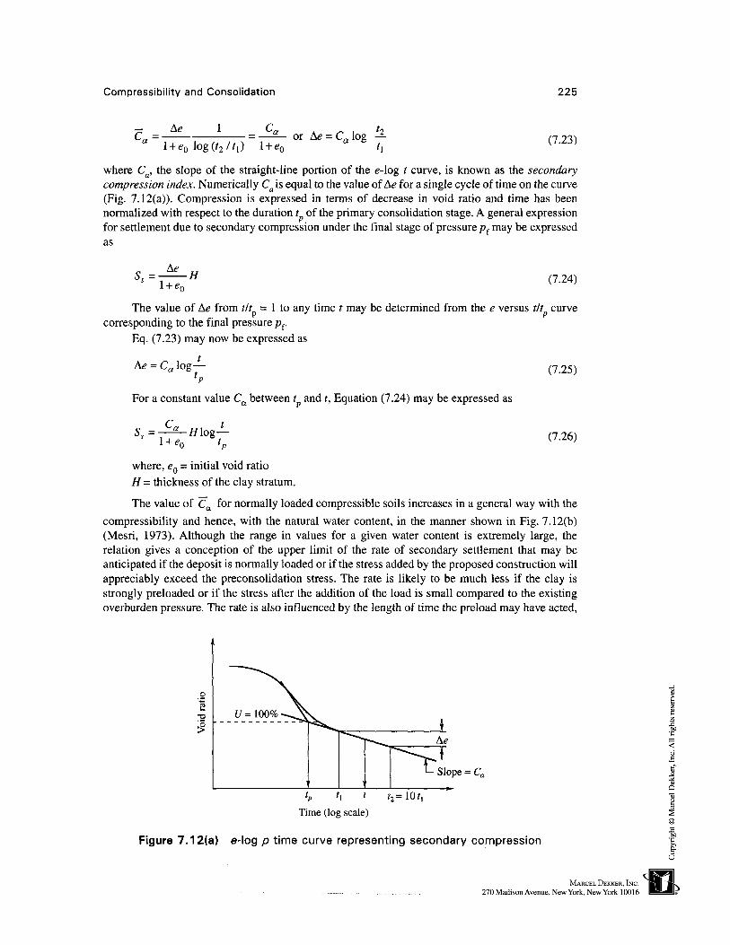
where Ca, the slope of the straight-line portion of the e-log t curve, is known as the secondarycompression index. Numerically Ca is equal to the value of Ae for a single cycle of time on the curve(Fig. 7.12(a)). Compression is expressed in terms of decrease in void ratio and time has beennormalized with respect to the duration t of the primary consolidation stage. A general expressionfor settlement due to secondary compression under the final stage of pressure pf may be expressedas

5 = •H (7.24)

The value of Ae from tit = 1 to any time / may be determined from the e versus tit curvecorresponding to the final pressure pf.

Eq. (7.23) may now be expressed as

A<? = Ca log —

For a constant value Ca between t and t, Equation (7.24) may be expressed as

(7.25)

(7.26)

where, eQ - initial void ratioH = thickness of the clay stratum.

The value of Ca for normally loaded compressible soils increases in a general way with the

compressibility and hence, with the natural water content, in the manner shown in Fig. 7.12(b)(Mesri, 1973). Although the range in values for a given water content is extremely large, therelation gives a conception of the upper limit of the rate of secondary settlement that may beanticipated if the deposit is normally loaded or if the stress added by the proposed construction willappreciably exceed the preconsolidation stress. The rate is likely to be much less if the clay isstrongly preloaded or if the stress after the addition of the load is small compared to the existingoverburden pressure. The rate is also influenced by the length of time the preload may have acted,

Slope = Ca

r 2 =10f ,

Time (log scale)

Figure 7.12(a) e-log p time curve representing secondary compression

226 Chapter 7

100

10

1.0-

0.110

1. Sensitive marine clay, NewZealand

2. Mexico city clay3. Calcareous organic clay4. Leda clay5. Norwegian plastic clay6. Amorphous and fibrous peat7. Canadian muskeg8. Organic marine deposits

9. Boston blue clay10. Chicago blue clay11. Organic silty clayO Organic silt, etc.

100Natural water content, percent

1000 3000

Figure 7.12(b) Relationship between coefficient of secondary consolidation andnatural water content of normally loaded deposits of clays and various compressible

organic soils (after Mesri, 1973)

by the existence of shearing stresses and by the degree of disturbance of the samples. The effects ofthese various factors have not yet been evaluated. Secondary compression is high in plastic claysand organic soils. Table 7.1 provides a classification of soil based on secondary compressibility. If'young, normally loaded clay', having an effective overburden pressure of p0 is left undisturbed forthousands of years, there will be creep or secondary consolidation. This will reduce the void ratioand consequently increase the preconsolidation pressure which will be much greater than theexisting effective overburden pressure pQ. Such a clay may be called an aged, normallyconsolidated clay.

Mesri and Godlewski (1977) report that for any soil the ratio Ca/Cc is a constant (where Cc isthe compression index). This is illustrated in Fig. 7.13 for undisturbed specimens of brown MexicoCity clay with natural water content wn = 313 to 340%, vv; = 361%, wp = 9\% andpc/po = 1.4

Table 7.2 gives values of Ca/Ccfor some geotechnical materials (Terzaghi, et al., 1996).It is reported (Terzaghi et al., 1996) that for all geotechnical materials Ca/Cc ranges from

0.01 to 0.07. The value 0.04 is the most common value for inorganic clays and silts.


0.3

0.2

•o§

0.1

i i

Mexico City clay

calcc = 0.046

0 1 2 3 4 5 6Compression index Cc

Figure 7.13 An example of the relation between Ca and Cc (after Mesri andGodlewski, 1977)

Table 7.1 Classification of soil based on secondary compressibility (Terzaghi,et al., 1996)

C Secondary compressibility

< 0.002

0.004

0.008

0.0160.0320.064

Very low

LowMedium

High

Very highExtremely high

Table 7.2 Values of CaICc for geotechnical materials (Terzaghi, et al., 1996)

Material

Granular soils including rockfill 0.02 ± 0.01

Shale and mudstone 0.03 ± 0.01

Inorganic clay and silts 0.04 ± 0.01

Organic clays and silts 0.05 ± 0.01

Peat and muskeg 0.06 ± 0.01

Example 7.1During a consolidation test, a sample of fully saturated clay 3 cm thick (= hQ) is consolidated undera pressure increment of 200 kN/m2. When equilibrium is reached, the sample thickness is reducedto 2.60 cm. The pressure is then removed and the sample is allowed to expand and absorb water.The final thickness is observed as 2.8 cm (ft,) and the final moisture content is determined as 24.9%.

228 Chapter 7

K, = 0.672 cm3

Figure Ex. 7.1

If the specific gravity of the soil solids is 2.70, find the void ratio of the sample before and afterconsolidation.

Solution

Use equation (7.3)

-h

A/z

1. Determination of 'e*

Weight of solids = Ws = VsGs Jm = 1 x 2.70 x 1 = 2.70 g.

W

W= 0.249 or Ww = 0.249 x 2.70 = 0.672 gm, ef = Vw= 0.672.

2. Changes in thickness from final stage to equilibrium stage with load on

(1 + 0.672)0.20A/i = 2.80 -2.60 = 0.20 cm,

2.80• = 0.119.

Void ratio after consolidation = e,- &e = 0.672 - 0.1 19 = 0.553.

3. Change in void ratio from the commencement to the end of consolidation

1 + 0-553(3.00 - 2.60) = x 0.40 = 0.239 .

2.6 2.6

Void ratio at the start of consolidation = 0.553 + 0.239 = 0.792

Example 7.2A recently completed fill was 32.8 ft thick and its initial average void ratio was 1.0. The fill wasloaded on the surface by constructing an embankment covering a large area of the fill. Somemonths after the embankment was constructed, measurements of the fill indicated an average voidratio of 0.8. Estimate the compression of the fill.


Solution

Per Eq. (7.7), the compression of the fill may be calculated as

where AH = the compression, Ae = change in void ratio, eQ = initial void ratio, HQ = thickness of fill.

Substituting, A/f = L0~0-8 x 32.8 = 3.28 ft .

Example 7.3A stratum of normally consolidated clay 7 m thick is located at a depth 12m below ground level.The natural moisture content of the clay is 40.5 per cent and its liquid limit is 48 per cent. Thespecific gravity of the solid particles is 2.76. The water table is located at a depth 5 m below groundsurface. The soil is sand above the clay stratum. The submerged unit weight of the sand is 1 1 kN/m3

and the same weighs 18 kN/m3 above the water table. The average increase in pressure at the centerof the clay stratum is 120 kN/m2 due to the weight of a building that will be constructed on the sandabove the clay stratum. Estimate the expected settlement of the structure.

Solution

1 . Determination of e and yb for the clay [Fig. Ex. 7.3]

W=1x2.76x1 = 2.76 g

405W = — x2.76 = 1.118 gw 100

„r

vs i= UI& + 2.76 = 3.878 g

W ' 1 Q - J / 3Y, = - = - = 1-83 g/cm' 2.118

Yb =(1.83-1) = 0.83 g/cm3.

2. Determination of overburden pressure pQ

PO = y\hi + Y2hi + yA °r

P0= 0.83x9.81x3.5 + 11x7 + 18x5 = 195.5 kN/m2

3. Compression index [Eq. 11.17]

Cc = 0.009(w, - 10) = 0.009 x (48 - 10) = 0.34

230 Chapter 7

w

w.

5 m

7m J

7 mI

(b)

Fig. Ex. 7.3

4. Excess pressure

A;? = 120 kN/m2

5. Total Settlement

Cst =

0.34 _ _ n i 195.5 + 120 000x 700 log = 23.3 cm2.118 " 195.5

Estimated settlement = 23.3 cm.

Example 7.4A column of a building carries a load of 1000 kips. The load is transferred to sub soil through a squarefooting of size 16 x 16 ft founded at a depth of 6.5 ft below ground level. The soil below the footingis fine sand up to a depth of 16.5 ft and below this is a soft compressible clay of thickness 16 ft. Thewater table is found at a depth of 6.5 ft below the base of the footing. The specific gravities of the solidparticles of sand and clay are 2.64 and 2.72 and their natural moisture contents are 25 and 40 percentrespectively. The sand above the water table may be assumed to remain saturated. If the plastic limitand the plasticity index of the clay are 30 and 40 percent respectively, estimate the probable settlementof the footing (see Fig. Ex. 7.4)

Solution

1. Required A/? at the middle of the clay layer using the Boussinesq equation

24.5

16= 1.53 < 3.0

Divide the footing into 4 equal parts so that Z/B > 3The concentrated load at the center of each part = 250 kips

Radial distance, r = 5.66 ftBy the Boussinesq equation the excess pressure A/? at depth 24.5 ft is (IB = 0.41)

0.41 = 0.683k/ft2

24.5'


. - . * ' . . •.•6.5 ft W.

CX

3

^^ferief,.

24.5 ft = Z

16ft

16ft - r = 5.66 ft

Figure Ex. 7.4

2. Void ratio and unit weights

Per the procedure explained in Ex. 7.3

For sand y, = 124 lb/ft3 yfc = 61.6 lb/ft3

For clay yb = 51.4 lb/ft3 <?0 = 1.09

3. Overburden pressure pQ

pQ = 8 x 51.4 + 10 x 62 + 13 x 124 = 2639 lb/ft2

4. Compression index

w/ = Ip + wp = 40 + 30 = 70%, Cc = 0.009 (70 - 10) = 0.54

0.54 ... . 2639 + 683 ft/liaA A 0, .Settlement S, = . ._x!6xlog = 0.413 ft = 4.96m.

1 + 1.09 2639

Example 7.5Soil investigation at a site gave the following information. Fine sand exists to a depth of 10.6 m andbelow this lies a soft clay layer 7.60 m thick. The water table is at 4.60 m below the ground surface.The submerged unit weight of sand yb is 10.4 kN/m3, and the wet unit weight above the water tableis 17.6 kN/m3. The water content of the normally consolidated clay wn = 40%, its liquid limitwt = 45%, and the specific gravity of the solid particles is 2.78. The proposed construction willtransmit a net stress of 120 kN/m2 at the center of the clay layer. Find the average settlement of theclay layer.

232 Chapter 7

Solution

For calculating settlement [Eq. (7.15a)]

C pn + A/?S = — — H log^ - - where &p = 120 kN / m2

l + eQ pQ

From Eq. (7.17), Cr = 0.009 (w, - 10) = 0.009(45 - 10) = 0.32

wGFrom Eq. (3. 14a), eQ = - = wG = 0.40 x 2.78 = 1.1 1 since S = 1

tJ

Yb, the submerged unit weight of clay, is found as follows

MG.+«.) = 9*1(2.78 + Ul) 3' ^"t 1 , 1 . 1 1 1l + eQ l + l.ll

Yb=Y^-Yw =18.1-9.81 = 8.28 kN/m 3

The effective vertical stress pQ at the mid height of the clay layer is

pQ = 4.60 x 17.6 + 6 x 10.4 + — x 8.28 = 174.8 kN / m2

_ 0.32x7.60, 174.8 + 120Now St = - log - = 0.26m = 26 cm1 1+1.11 174.8Average settlement = 26 cm.

Example 7.6A soil sample has a compression index of 0.3. If the void ratio e at a stress of 2940 Ib/ft2 is 0.5,compute (i) the void ratio if the stress is increased to 4200 Ib/ft2, and (ii) the settlement of a soilstratum 13 ft thick.

Solution

Given: Cc = 0.3, el = 0.50, /?, = 2940 Ib/ft2, p2 = 4200 Ib/ft2.(i) Now from Eq. (7.4),

p — pC i %."-)

C = l- 2—

or e2 = e]-c

substituting the known values, we have,

e- = 0.5 - 0.31og - 0.4542 2940

(ii) The settlement per Eq. (7.10) is

c cc „, Pi 0.3x13x12, 4200S = — — //log— = - log - = 4.83 m.

pl 1.5 2940


Example 7.7Two points on a curve for a normally consolidated clay have the following coordinates.

Point 1 : *, = 0.7, Pl = 2089 lb/ft2

Point 2: e2 = 0.6, p2 = 6266 lb/ft2

If the average overburden pressure on a 20 ft thick clay layer is 3133 lb/ft2, how muchsettlement will the clay layer experience due to an induced stress of 3340 lb/ft2 at its middepth.

SolutionFrom Eq. (7.4) we have

C - e^e> = °-7"a6 -021c \ogp2/pl log (6266/2089)

We need the initial void ratio eQ at an overburden pressure of 3133 lb/ft2.

en -e~C =—2 — T2— = 0.21

or (eQ - 0.6) = 0.21 log (6266/3 133) = 0.063or eQ = 0.6 + 0.063 = 0.663.

Settlement, s =Po

Substituting the known values, with Ap = 3340 lb/ft2

„ 0.21x20x12, 3133 + 3340 nee.$ = - log - = 9.55 in1.663 & 3133

7.10 RATE OF ONE-DIMENSIONAL CONSOLIDATION THEORY OFTERZAGHIOne dimensional consolidation theory as proposed by Terzaghi is generally applicable in all casesthat arise in practice where

1. Secondary compression is not very significant,2. The clay stratum is drained on one or both the surfaces,3. The clay stratum is deeply buried, and4. The clay stratum is thin compared with the size of the loaded areas.

The following assumptions are made in the development of the theory:

1. The voids of the soil are completely filled with water,2. Both water and solid constituents are incompressible,3. Darcy's law is strictly valid,4. The coefficient of permeability is a constant,5. The time lag of consolidation is due entirely to the low permeability of the soil, and6. The clay is laterally confined.

234 Chapter 7

Differential Equation for One-Dimensional Flow

Consider a stratum of soil infinite in extent in the horizontal direction (Fig. 7.14) but of suchthickness //, that the pressures created by the weight of the soil itself may be neglected incomparison to the applied pressure.

Assume that drainage takes place only at the top and further assume that the stratum has beensubjected to a uniform pressure of pQ for such a long time that it is completely consolidated underthat pressure and that there is a hydraulic equilibrium prevailing, i.e., the water level in thepiezometric tube at any section XY in the clay stratum stands at the level of the water table(piezometer tube in Fig. 7.14).

Let an increment of pressure A/? be applied. The total pressure to which the stratum issubjected is

Pl=pQ + Ap (7.27)

Immediately after the increment of load is applied the water in the pore space throughout theentire height, H, will carry the additional load and there will be set up an excess hydrostaticpressure ui throughout the pore water equal to Ap as indicated in Fig. 7.14.

After an elapsed time t = tv some of the pore water will have escaped at the top surface and as aconsequence, the excess hydrostatic pressure will have been decreased and a part of the load transferred tothe soil structure. The distribution of the pressure between the soil and the pore water, p and u respectivelyat any time t, may be represented by the curve as shown in the figure. It is evident that

Pi=p + u (7.28)

at any elapsed time t and at any depth z, and u is equal to zero at the top. The pore pressure u, at anydepth, is therefore a function of z and / and may be written as

u =f(z, t) (7.29)

Piezometers

Impermeable

(a) (b)

Figure 7.14 One-dimensional consolidation


Consider an element of volume of the stratum at a depth z, and thickness dz (Fig. 7.14). Letthe bottom and top surfaces of this element have unit area.

The consolidation phenomenon is essentially a problem of non-steady flow of water through aporous mass. The difference between the quantity of water that enters the lower surface at level X'Y'and the quantity of water which escapes the upper surface at level XY in time element dt must equal thevolume change of the material which has taken place in this element of time. The quantity of water isdependent on the hydraulic gradient which is proportional to the slope of the curve t .

The hydraulic gradients at levels XY and X'Y' of the element are

, 1 d du 1 du ̂ 1 d2u ,iss^-*u+** =TwTz+Tw^dz (7-30)

If k is the hydraulic conductivity the outflow from the element at level XY in time dt is

k dudql=ikdt = ——dt (7.31)

' W **

The inflow at level X'Y' is

k du d2udq2 = ikdt = ~^dt + -^dzdt (7.32)

The difference in flow is therefore

kdq = dq^ -dq2 = -— -r-^dz dt (7.33)

• w

From the consolidation test performed in the laboratory, it is possible to obtain therelationship between the void ratios corresponding to various pressures to which a soil is subjected.This relationship is expressed in the form of a pressure-void ratio curve which gives therelationship as expressed in Eq. (7.12)

de = avdp (7.34)

The change in volume Adv of the element given in Fig. 7.14 may be written as perEq. (7.7).

deMv = Mz = - - dz (7.35)

i + e

Substituting for de, we have

(7.36)

Here dp is the change in effective pressure at depth z during the time element dt. The increasein effective pressure dp is equal to the decrease in the pore pressure, du.

duTherefore, dp = -du = -^~dt (7.37)

at

236 Chapter 7

av du duHence, Mv = — — dtdz = -tnv—dtdz (7.38)

l + e at v dt v '

Since the soil is completely saturated, the volume change AJv of the element of thicknessdz in time dt is equal to the change in volume of water dq in the same element in time dt.

Therefore, dq = Mv (7.39)

or

or

k d2u-, -, di Lrw di2

k(\ + e}d2u

Ywav dz2

a du-it -i -ifu — , ^ az atl + e dt

dt v dz2

ky a y m' W V ' W V

is defined as the coefficient of consolidation.

(7.40)

(7.41)

Eq. (7.40) is the differential equation for one-dimensional flow. The differential equation forthree-dimensional flow may be developed in the same way. The equation may be written as

du l + e d2u d2u d2u(7'42)

where kx, ky and kz are the coefficients of permeability (hydraulic conductivity) in the coordinatedirections of jc, y and z respectively.

As consolidation proceeds, the values of k, e and av all decrease with time but the ratioexpressed by Eq. (7.41) may remain approximately constant.

Mathematical Solution for the One-Dimensional Consolidation Equation

To solve the consolidation Eq. (7.40) it is necessary to set up the proper boundary conditions. Forthis purpose, consider a layer of soil having a total thickness 2H and having drainage facilities atboth the top and bottom faces as shown in Fig. 7.15. Under this condition no flow will take placeacross the center line at depth H. The center line can therefore be considered as an imperviousbarrier. The boundary conditions for solving Eq. (7.40) may be written as

1 . u = 0 when z = 02. u = 0 when z = 2H

3. u = <\p for all depths at time t = 0

On the basis of the above conditions, the solution of the differential Eq. (7.40) can beaccomplished by means of Fourier Series.

The solution is

mz _m2 ru= - sin — e ml (7.43)

m H

1)* cvt .where m - - , / = — — = a non-dimensional time factor.

2 H2

Eq. (7.43) can be expressed in a general form as


H

H

Clay

'• Sand y..'•:.': I

P\

Figure 7.15 Boundary conditions

~Kp=f~H'T (7'44)

Equation (7.44) can be solved by assuming T constant for various values of z/H. Curvescorresponding to different values of the time factor T may be obtained as given in Fig. 7.16. It is ofinterest to determine how far the consolidation process under the increment of load Ap has progressedat a time t corresponding to the time factor T at a given depth z. The term £/, is used to express thisrelationship. It is defined as the ratio of the amount of consolidation which has already taken place tothe total amount which is to take place under the load increment.

The curves in Fig. 7.16 shows the distribution of the pressure Ap between solid and liquid phasesat various depths. At a particular depth, say z/H = 0.5, the stress in the soil skeleton is represented by ACand the stress in water by CB. AB represents the original excess hydrostatic pressure ui = Ap. The degreeof consolidation Uz percent at this particular depth is then

AC Ap-« uu % = ioox—- = -t-— = 100 i-—z AB Ap Ap (7.45)

r1.0

A/7- U

0.5

z/H 1.0

r=o1.5

2.0

T= oo

Figure 7.16 Consolidation of clay layer as a function T

238 Chapter 7

Following a similar reasoning, the average degree of consolidation U% for the entire layer ata time factor Tis equal to the ratio of the shaded portion (Fig. 7.16) of the diagram to the entire areawhich is equal to 2H A/?.

Therefore

2H

U% = u _.. xlOO

2H

or £/% = 2H—— udz2H ^p

o

Hence, Eq. (7.46) after integration reduces to

(7.46)

£/%=100 1- —-£ -m2T(7.47)

It can be seen from Eq. (7.47) that the degree of consolidation is a function of the time factor Tonly which is a dimensionless ratio. The relationship between Tand U% may therefore be establishedonce and for all by solving Eq. (7.47) for various values of T. Values thus obtained are given inTable 7.3 and also plotted on a semilog plot as shown in Fig. 7.17.

For values of U% between 0 and 60%, the curve in Fig. 7.17 can be represented almostexactly by the equation

T =4 100

which is the equation of a parabola. Substituting for T, Eq. (7.48) may be written as

U%

oo

(7.48)

(7.49)

u%

u

20

40

60

80

100O.C

— • — „

--\\,

k\

\

^^)03 0.01 0.03 0.1 0.3 1.0 3.0 10

Time factor T(log scale)

Figure 7.17 U versus T


Table 7.3 Relationship between U and T

u%0

10

15

20

25

30

35

T

0

0.0080.018

0.031

0.0490.071

0.096

U%

40

45

50

55

60

65

70

T

0.126

0.159

0.197

0.2380.2870.3420.405

U%

75

80

85

90

95

100

T

0.4770.5650.6840.8481.127oo

In Eq. (7.49), the values of cv and H are constants. One can determine the time required toattain a given degree of consolidation by using this equation. It should be noted that H representshalf the thickness of the clay stratum when the layer is drained on both sides, and it is the fullthickness when drained on one side only.

TABLE 7.4 Relation between U% and T (Special Cases)

Permeable Permeable

U%

ImpermeableCase 1

ImpermeableCase 2

Time Factors, T

Consolidation pressureincrease with depth

Consolidation pressuredecreases with depth

00

10

20

30

40

50

60

70

80

90

95

100

0

0.047

0.100

0.158

0.221

0.294

0.383

0.500

0.665

0.94

1oo

0

0.003

0.0090.024

0.0480.092

0.160

0.271

0.44

0.72

0.8oo

240 Chapter 7

For values of U% greater than 60%, the curve in Fig. 7.17 may be represented by the equation

T= 1.781 - 0.933 log (100 - U%) (7.50)

Effect of Boundary Conditions on Consolidation

A layer of clay which permits drainage through both surfaces is called an open layer. The thicknessof such a layer is always represented by the symbol 2H, in contrast to the symbol H used for thethickness of half-closed layers which can discharge their excess water only through one surface.

The relationship expressed between rand (/given in Table 7.3 applies to the following cases:

1. Where the clay stratum is drained on both sides and the initial consolidation pressuredistribution is uniform or linearly increasing or decreasing with depth.

2. Where the clay stratum is drained on one side but the consolidation pressure is uniformwith depth.

Separate relationships between T and U are required for half closed layers with thickness Hwhere the consolidation pressures increase or decrease with depth. Such cases are exceptional andas such not dealt with in detail here. However, the relations between U% and 7" for these two casesare given in Table 7.4.

7.11 DETERMINATION OF THE COEFFICIENT OF CONSOLIDATIONThe coefficient of consolidation c can be evaluated by means of laboratory tests by fitting theexperimental curve with the theoretical.

There are two laboratory methods that are in common use for the determination of cv. Theyare

1. Casagrande Logarithm of Time Fitting Method.2. Taylor Square Root of Time Fitting Method.

Logarithm of Time Fitting Method

This method was proposed by Casagrande and Fadum (1940).Figure 7.18 is a plot showing the relationship between compression dial reading and the

logarithm of time of a consolidation test. The theoretical consolidation curve using the log scale forthe time factor is also shown. There is a similarity of shape between the two curves. On thelaboratory curve, the intersection formed by the final straight line produced backward and thetangent to the curve at the point of inflection is accepted as the 100 per cent primary consolidationpoint and the dial reading is designated as /?100. The time-compression relationship in the earlystages is also parabolic just as the theoretical curve. The dial reading at zero primary consolidationRQ can be obtained by selecting any two points on the parabolic portion of the curve where times arein the ratio of 1 : 4. The difference in dial readings between these two points is then equal to thedifference between the first point and the dial reading corresponding to zero primary consolidation.For example, two points A and B whose times 10 and 2.5 minutes respectively, are marked on thecurve. Let z{ be the ordinate difference between the two points. A point C is marked vertically overB such that BC = zr Then the point C corresponds to zero primary consolidation. The procedure isrepeated with several points. An average horizontal line is drawn through these points to representthe theoretical zero percent consolidation line.

The interval between 0 and 100% consolidation is divided into equal intervals of percentconsolidation. Since it has been found that the laboratory and the theoretical curves have better


Asymptote

Rf\-

f i/4 t} log (time)

(a) Experimental curve (b) Theoretical curve

Figure 7.18 Log of time fitting method

correspondence at the central portion, the value of cy is computed by taking the time t and timefactor T at 50 percent consolidation. The equation to be used is

T-~Hlr (7.51)

T -15Q

c tv 50 orldr

where Hdr = drainage pathFrom Table 7.3, we have at U = 50%, T= 0.197. From the initial height //. of specimen and

compression dial reading at 50% consolidation, Hdr for double drainage is

H: ~

(7.52)

where hH= Compression of sample up to 50% consolidation.Now the equation for c may be written as

c = 0.197H

(7.53)

Square Root of Time Fitting Method

This method was devised by Taylor (1948). In this method, the dial readings are plotted against the

square root of time as given in Fig. 7.19(a). The theoretical curve U versus ^JT is also plotted andshown in Fig. 7.19(b). On the theoretical curve a straight line exists up to 60 percent consolidationwhile at 90 percent consolidation the abscissa of the curve is 1.15 times the abscissa of the straightline produced.

The fitting method consists of first drawing the straight line which best fits the early portion of thelaboratory curve. Next a straight line is drawn which at all points has abscissa 1.15 times as great as thoseof the first line. The intersection of this line and the laboratory curve is taken as the 90 percent (RQQ)consolidation point. Its value may be read and is designated as tgQ.

242 Chapter 7

(a) Experimental curve (b) Theoretical curve

Figure 7.19 Square root of time fitting method

Usually the straight line through the early portion of the laboratory curve intersects the zerotime line at a point (Ro) differing somewhat from the initial point (/?f.). This intersection point iscalled the corrected zero point. If one-ninth of the vertical distance between the corrected zeropoint and the 90 per cent point is set off below the 90 percent point, the point obtained is called the"100 percent primary compression point" (Rloo). The compression between zero and 100 per centpoint is called "primary compression".

At the point of 90 percent consolidation, the value of T = 0.848. The equation of cv may nowbe written as

H2

c =0.848-^ (7.54)'90

where H, - drainage path (average)

7.12 RATE OF SETTLEMENT DUE TO CONSOLIDATIONIt has been explained that the ultimate settlement St of a clay layer due to consolidation may becomputed by using either Eq. (7.10) or Eq. (7.13). If S is the settlement at any time t after theimposition of load on the clay layer, the degree of consolidation of the layer in time t may beexpressed as

U% = — x 100 percent

Since U is a function of the time factor T, we may write

(7.55)

= — x l O OO

(7.56)

The rate of settlement curve of a structure built on a clay layer may be obtained by thefollowing procedure:


Time t

Figure 7.20 Time-settlement curve

1. From consolidation test data, compute mv and cv.

2. Compute the total settlement St that the clay stratum would experience with the incrementof load Ap.

3. From the theoretical curve giving the relation between U and T, find T for different degreesof consolidation, say 5, 10, 20, 30 percent etc.

TH2,4. Compute from equation t = —— the values of t for different values of T. It may be noted

Cv

here that for drainage on both sides Hdr is equal to half the thickness of the clay layer.5. Now a curve can be plotted giving the relation between t and U% or t and S as shown in

Fig. 7.20.

7.13 TWO- AND THREE-DIMENSIONAL CONSOLIDATIONPROBLEMSWhen the thickness of a clay stratum is great compared with the width of the loaded area, theconsolidation of the stratum is three-dimensional. In a three-dimensional process of consolidationthe flow occurs either in radial planes or else the water particles travel along flow lines which do notlie in planes. The problem of this type is complicated though a general theory of three-dimensionalconsolidation exists (Biot, et al., 1941). A simple example of three-dimensional consolidation is theconsolidation of a stratum of soft clay or silt by providing sand drains and surcharge foraccelerating consolidation.

The most important example of two dimensional consolidation in engineering practice is theconsolidation of the case of a hydraulic fill dam. In two-dimensional flow, the excess water drainsout of the clay in parallel planes. Gilboy (1934) has analyzed the two dimensional consolidation ofa hydraulic fill dam.

Example 7.8A 2.5 cm thick sample of clay was taken from the field for predicting the time of settlement for aproposed building which exerts a uniform pressure of 100 kN/m2 over the clay stratum. The samplewas loaded to 100 kN/m2 and proper drainage was allowed from top and bottom. It was seen that 50percent of the total settlement occurred in 3 minutes. Find the time required for 50 percent of the

244 Chapter 7

total settlement of the building, if it is to be constructed on a 6 m thick layer of clay which extendsfrom the ground surface and is underlain by sand.

Solution

Tfor 50% consolidation = 0.197.

The lab sample is drained on both sides. The coefficient of consolidation c is found from

TH2 (2 5)2 1c = — = 0.197 x —— x - = 10.25 x 10~2 cm2 / min.

t 4 3

The time t for 50% consolidation in the field will be found as follows.

0.197x300x300x100 , „ „ _ ,t = : = 120 days.

10.25x60x24

Example 7.9The void ratio of a clay sample A decreased from 0.572 to 0.505 under a change in pressure from122 to 180 kN/m2. The void ratio of another sample B decreased from 0.61 to 0.557 under the sameincrement of pressure. The thickness of sample A was 1.5 times that of B. Nevertheless the timetaken for 50% consolidation was 3 times larger for sample B than for A. What is the ratio ofcoefficient of permeability of sample A to that of Bl

Solution

Let Ha = thickness of sample A, Hb = thickness of sample B, mva = coefficient of volumecompressibility of sample A, mvb = coefficient of volume compressibility of sample B, cva =coefficient of consolidation for sample A, cvb = coefficient of consolidation for sample B, A/?a =increment of load for sample A, A/?fe = increment of load for sample B, ka = coefficient ofpermeability for sample A, and kb = coefficient of permeability of sample B.

We may write the following relationship

Ae 1 A<?, lm = - a- -- —,mh= -

b- -- —va \ + e Aw vb l + e, Ap,a * a b rb

where e is the void ratio of sample A at the commencement of the test and Aea is the change in voidratio. Similarly eb and keb apply to sample B.

-, and T =^K T, = ^fy-

wherein Ta, ta, Tb and tb correspond to samples A and B respectively. We may write

c T H2 t,— = "F^p *« = cvamvarw> kb = cvbm

vbywvb b b a

k c m™ r. a va vaTherefore, k c m

b vb vb

Given ea = 0.572, and eb = 0.61

A<? = 0.572-0.505 = 0.067, Ae. =0.610-0.557 = 0.053a ' o


A D = Ap, = 180-122 = 58kN/m2, H=l.5H,

But tb = 3ta

Q.Q67 1 + 0.61a

We have, m = 0.053 * 1 + 0.572 = L29

vb

kTherefore, T2-= 6.75 x 1.29 = 8.7

KbThe ratio is 8.7 : 1.

Example 7.10A strata of normally consolidated clay of thickness 10 ft is drained on one side only. It has ahydraulic conductivity of h = 1.863 x 10~8 in/sec and a coefficient of volume compressibilityrav = 8.6 x 10"4 in2/lb. Determine the ultimate value of the compression of the stratum by assuminga uniformly distributed load of 5250 lb/ft2 and also determine the time required for 20 percent and80 percent consolidation.

Solution

Total compression,

S = m //A/? = 8.6 x 10~4 x 10 x 12 x 5250 x — = 3.763 in.< v f 144

For determining the relationship between U% and T for 20% consolidation use the equation

n U% 2 3.14 20 2

T = ̂ m orT = ~xm =a°314

For 80% consolidation use the equation

T = 1.781 - 0.933 log (100 - £/%)

Therefore T= 1.781 - 0.933 Iog10 (100 - 80) = 0.567.

The coefficient of consolidation is

k 1.863xlO~8 , m 4 • ? /c = = - 6 x 10~4 in2 / secywmv 3.61xlO~2x8.

The times required for 20% and 80% consolidation are

H2drT (10xl2)2x0.0314

f2o = —££L— = ~A = 8.72 dayscv 6xlO" 4x60x60x24

H2drT (10 x!2)2x 0.567?so = = A = 157.5 days

cv 6xlO" 4x60x60x24

246 Chapter 7

Example 7.11

The loading period for a new building extended from May 1995 to May 1997. In May 2000, theaverage measured settlement was found to be 11.43 cm. It is known that the ultimate settlement willbe about 35.56 cm. Estimate the settlement in May 2005. Assume double drainage to occur.

Solution

For the majority of practical cases in which loading is applied over a period, acceptable accuracy isobtained when calculating time-settlement relationships by assuming the time datum to be midwaythrough the loading or construction period.

St = 11.43 cm when t = 4 years and 5 = 35.56 cm.

The settlement is required for t = 9 years, that is, up to May2005. Assuming as a starting pointthat at t = 9 years, the degree of consolidation will be = 0.60. Under these conditions per Eq. (7.48),U= 1.13 Vl

If St = settlement at time t,, S, = settlement at time t,' l

= — sinceH2

dr

IT°r ~ cm

_where ~~ is a constant. Therefore ~T ~ A o" '2

VL ^ , 1 -*Hdr h

17.5Therefore at t = 9 years, U = 7777 = 0.48

35.56

Since the value of U is less than 0.60 the assumption is valid. Therefore the estimatedsettlement is 17.15 cm. In the event of the degree of consolidation exceeding 0.60, equation (7.50)has to be used to obtain the relationship between T and U.

Example 7.12An oedometer test is performed on a 2 cm thick clay sample. After 5 minutes, 50% consolidation isreached. After how long a time would the same degree of consolidation be achieved in the fieldwhere the clay layer is 3.70 m thick? Assume the sample and the clay layer have the same drainageboundary conditions (double drainage).

Solution

c,.tThe time factor T is defined as T -

where Hdr - half the thickness of the clay for double drainage.Here, the time factor T and coefficient of consolidation are the same for both the sample and

the field clay layer. The parameter that changes is the time /. Let tl and t2 be the times required toreach 50% consolidation both in the oedometer and field respectively. t{ = 5 min

=

Therefore t/2 t/2ndr(\) ndr(2)

2 jH, n, 3 7 0 1 1

Now fi = t,= x5x — x—days ~ 119 days.WOW 2 Hd ' 2 6 0 2 4 y


Example 7.13A laboratory sample of clay 2 cm thick took 15 min to attain 60 percent consolidation under adouble drainage condition. What time will be required to attain the same degree of consolidationfor a clay layer 3 m thick under the foundation of a building for a similar loading and drainagecondition?

Solution

Use Eq. (7.50) for U > 60% for determining T

T= 1.781-0.933 log(l00-£/%)

= 1.781-0.933 log (100-60) = 0.286.

From Eq. (7.51) the coefficient of consolidation, cv is

TH2 0.286 x (I)2

c = • = 1.91xlO~2 cm2/min.15

The value of cv remains constant for both the laboratory and field conditions. As such, wemay write,

lab \ J field

where Hdr - half the thickness = 1 cm for the lab sample and 150cm for field stratum, and15 min.Therefore,

tlab = 15 min.

or tf= (150)2 x 0.25 = 5625 hr or 234 days (approx).for the field stratum to attain the same degree of consolidation.

7.14 PROBLEMS7.1 A bed of sand 10m thick is underlain by a compressible of clay 3 m thick under which lies

sand. The water table is at a depth of 4 m below the ground surface. The total unit weightsof sand below and above the water table are 20.5 and 17.7 kN/m3 respectively. The clay hasa natural water content of 42%, liquid limit 46% and specific gravity 2.76. Assuming theclay to be normally consolidated, estimate the probable final settlement under an averageexcess pressure of 100 kN/m2.

7.2 The effective overburden pressure at the middle of a saturated clay layer 12 ft thick is2100 lb/ft2 and is drained on both sides. The overburden pressure at the middle of the claystratum is expected to be increased by 3150 lb/ft2 due to the load from a structure at theground surface. An undisturbed sample of clay 20 mm thick is tested in a consolidometer.The total change in thickness of the specimen is 0.80 mm when the applied pressure is2100 lb/ft2. The final water content of the sample is 24 percent and the specific gravity ofthe solids is 2.72. Estimate the probable final settlement of the proposed structure.

248 Chapter 7

7.3 The following observations refer to a standard laboratory consolidation test on anundisturbed sample of clay.

Pressure

kN/m2

0

50

100

200

Final Dial Gauge

Reading x 10~2 mm

0

180

250

360

Pressure

kN/m2

400

100

0

Final Dial Gauge

Reading x 10~2 mm

520

470

355

The sample was 75 mm in diameter and had an initial thickness of 18 mm. The moisturecontent at the end of the test was 45.5%; the specific gravity of solids was 2.53.Compute the void ratio at the end of each loading increment and also determine whetherthe soil was overconsolidated or not. If it was overconsolidated, what was theoverconsolidation ratio if the effective overburden pressure at the time of sampling was60 kN/m2?

7.4 The following points are coordinates on a pressure-void ratio curve for an undisturbed clay.

p 0.5 1 2 4 8 16 kips/ft2

e 1.202 1.16 1.06 0.94 0.78 0.58

Determine (i) Cc, and (ii) the magnitude of compression in a 10 ft thick layer of this clay fora load increment of 4 kips/ft2. Assume eQ = 1.320, andp0 =1.5 kips/ft2

7.5 The thickness of a compressible layer, prior to placing of a fill covering a large area, is 30ft. Its original void ratio was 1.0. Sometime after the fill was constructed measurementsindicated that the average void ratio was 0.8. Determine the compression of the soil layer.

7.6 The water content of a soft clay is 54.2% and the liquid limit is 57.3%. Estimate thecompression index, by equations (7.17) and (7.18). Given eQ = 0.85

7.7 A layer of normally consolidated clay is 20 ft thick and lies under a recently constructedbuilding. The pressure of sand overlying the clay layer is 6300 lb/ft2, and the new constructionincreases the overburden pressure at the middle of the clay layer by 2100 lb/ft2. If thecompression index is 0.5, compute the final settlement assuming vvn = 45%, Gs = 2.70, and theclay is submerged with the water table at the top of the clay stratum.

7.8 A consolidation test was made on a sample of saturated marine clay. The diameter andthickness of the sample were 5.5 cm and 3.75 cm respectively. The sample weighed 650 gat the start of the test and 480 g in the dry state after the test. The specific gravity of solidswas 2.72. The dial readings corresponding to the final equilibrium condition under eachload are given below.

Pressure, kN/m2

0

6.7

11.3

26.6

53.3

DR cm x 10~4

0

175

275

540

965

Pressure, kN/m2

106

213

426

852

£>/?cm x 10-4

1880

3340

5000

6600

(a) Compute the void ratios and plot the e-\og p curve.(b) Estimate the maximum preconsolidation pressure by the Casagrande method.(c) Draw the field curve and determine the compression index.


7.9 The results of a consolidation test on a soil sample for a load increased from 200 to400 kN/m2 are given below:

Time in Min .

0

0.10

0.25

0.50

1.00

2.25

4.00

9.00

Dial reading division

1255

1337

1345

1355

1384

1423

1480

1557

Time in Min .

1625

36

49

64

81

100

121

Dial reading division

1603

1632

1651

1661

1670

1677

1682

1687

The thickness of the sample corresponding to the dial reading 1255 is 1.561 cm. Determinethe value of the coefficient of consolidation using the square root of time fitting method incm2/min. One division of dial gauge corresponds to 2.5 x lO^4 cm. The sample is drainedon both faces.

7.10 A 2.5 cm thick sample was tested in a consolidometer under saturated conditions withdrainage on both sides. 30 percent consolidation was reached under a load in15 minutes. For the same conditions of stress but with only one way drainage, estimate thetime in days it would take for a 2 m thick layer of the same soil to consolidate in the field toattain the same degree of consolidation.

7.11 The dial readings recorded during a consolidation test at a certain load increment are givenbelow.

Time

min

0

0.10

0.25

0.50

1.00

2.00

4.00

8.00

Dial Reading

cm x 10~4

240

318

340

360

385

415

464

530

Time

min

15

30

60

120

240

1200

-

Dial Reading

cm x 10~4

622

738

842

930

975

1070

-

Determine cv by both the square root of time and log of time fitting methods. The thicknessof the sample at DR 240 = 2 cm and the sample is drained both sides.

7.12 In a laboratory consolidation test a sample of clay with a thickness of 1 in. reached 50%consolidation in 8 minutes. The sample was drained top and bottom. The clay layer fromwhich the sample was taken is 25 ft thick. It is covered by a layer of sand through whichwater can escape and is underlain by a practically impervious bed of intact shale. How longwill the clay layer require to reach 50 per cent consolidation?

7.13 The following data were obtained from a consolidation test performed on an undisturbedclay sample 3 cm in thickness:(i) pl = 3.5 kips/ft2, e{= 0.895

(ii) p2 = 6.5 kips/ft2, e2 = 0.782

250 Chapter 7

By utilizing the known theoretical relationship between percent consolidation and timefactor, compute and plot the decrease in thickness with time for a 10 ft thick layer of thisclay, which is drained on the upper surface only. Given : eQ = 0.92 /?0 = 4.5 kips/ft2,Ap = 1.5 kips/ft2, c , = 4.2 x 10~5 ft2/min.

7.14 A structure built on a layer of clay settled 5 cm in 60 days after it was built. If this settlementcorresponds to 20 percent average consolidation of the clay layer, plot the time settlementcurve of the structure for a period of 3 years from the time it was built. Given : Thickness ofclay layer = 3m and drained on one side

7.15 A 30 ft thick clay layer with single drainage settles 3.5 in. in 3.5 yr. The coefficientconsolidation for this clay was found to be 8.43 x 10"4 in.2/sec. Compute the ultimateconsolidation settlement and determine how long it will take to settle to 90% of thisamount.

7.16 The time factor T for a clay layer undergoing consolidation is 0.2. What is the averagedegree of consolidation (consolidation ratio) for the layer?

7.17 If the final consolidation settlement for the clay layer in Prob. 7.16 is expected to be 1.0 m,how much settlement has occurred when the time factor is (a) 0.2 and (b) 0.7?

7.18 A certain compressible layer has a thickness of 12 ft. After 1 yr when the clay is 50%consolidated, 3 in. of settlement has occurred. For similar clay and loading conditions, howmuch settlement would occur at the end of 1 yr and 4 yr, if the thickness of this new layerwere 20 ft?

7.19 A layer of normally consolidated clay 14 ft thick has an average void ratio of 1.3. Itscompression index is 0.6. When the induced vertical pressure on the clay layer is doubled,what change in thickness of the clay layer will result? Assume: pQ = 1200 lb/ft2 andA/? = 600 lb/ft2.

7.20 Settlement analysis for a proposed structure indicates that 2.4 in. of settlement will occur in4 yr and that the ultimate total settlement will be 9.8 in. The analysis is based on theassumption that the compressible clay layer is drained on both sides. However, it issuspected that there may not be drainage at the bottom surface. For the case of singledrainage, estimate the time required for 2.4 in. of settlement.

7.21 The time to reach 60% consolidation is 32.5 sec for a sample 1.27 cm thick tested in alaboratory under conditions of double drainage. How long will the corresponding layer innature require to reach the same degree of consolidation if it is 4.57 m thick and drained onone side only?

7.22 A certain clay layer 30 ft thick is expected to have an ultimate settlement of 16 in. If thesettlement was 4 in. after four years, how much longer will it take to obtain a settlement of6 in?

7.23 If the coefficient of consolidation of a 3 m thick layer of clay is 0.0003 cm2/sec, what is theaverage consolidation of that layer of clay (a) in one year with two-way drainage, and (b)the same as above for one-way drainage.

7.24 The average natural moisture content of a deposit is 40%; the specific gravity of the solidmatter is 2.8, and the compression index Cc is 0.36. If the clay deposit is 6.1 m thickdrained on both sides, calculate the final consolidation settlement St. Given: pQ = 60 kN/m2

and A/? = 30 kN/m2

7.25 A rigid foundation block, circular in plan and 6 m in diameter rests on a bed of compactsand 6 m deep. Below the sand is a 1.6 m thick layer of clay overlying on impervious bedrock. Ground water level is 1.5 m below the surface of the sand. The unit weight of sandabove water table is 19.2 kN/m3, the saturated unit weight of sand is 20.80 kN/m3, and thesaturated unit weight of the clay is 19.90 kN/m3.


A laboratory consolidation test on an undisturbed sample of the clay, 20 mm thick anddrained top and bottom, gave the following results:

Pressure (kN/m2) 50 100 200 400 800Void ratio 0.73 0.68 0.625 0.54 0.41

If the contact pressure at the base of the foundation is 200 kN/m2, and eQ = 0.80,calculate the final average settlement of the foundation assuming 2:1 method for thespread of the load.

7.26 A stratum of clay is 2 m thick and has an initial overburden pressure of 50 kN/m2 at themiddle of the clay layer. The clay is overconsolidated with a preconsolidation pressure of75 kN/m2. The values of the coefficients of recompression and compression indices are0.05 and 0.25 respectively. Assume the initial void ratio eQ = 1.40. Determine the finalsettlement due to an increase of pressure of 40 kN/m2 at the middle of the clay layer.

7.27 A clay stratum 5 m thick has the initial void ration of 1.50 and an effective overburdenpressure of 120 kN/m2. When the sample is subjected to an increase of pressure of120 kN/m2, the void ratio reduces to 1.44. Determine the coefficient of volumecompressibility and the final settlement of the stratum.

7.28 A 3 m thick clay layer beneath a building is overlain by a permeable stratum and isunderlain by an impervious rock. The coefficient of consolidation of the clay was found tobe 0.025 cm2/min. The final expected settlement for the layer is 8 cm. Determine (a) howmuch time will it take for 80 percent of the total settlement, (b) the required time for asettlement of 2.5 cm to occur, and (c) the settlement that would occur in one year.

7.29 An area is underlain by a stratum of clay layer 6 m thick. The layer is doubly drained andhas a coefficient of consolidation of 0.3 m2/month. Determine the time required for asurcharge load to cause a settlement of 40 cm if the same load cause a final settlement of60cm.

7.30 In an oedometer test, a clay specimen initially 25 mm thick attains 90% consolidation in10 minutes. In the field, the clay stratum from which the specimen was obtained has athickness of 6 m and is sandwiched between two sand layers. A structure constructed onthis clay experienced an ultimate settlement of 200 mm. Estimate the settlement at the endof 100 days after construction.

chapter 7civilwares.free.fr/geotechnical engineering - principles and... · 212 chapter 7 pressure...

Documents