chapter 9wellsmat.startlogic.com/.../sitebuilderfiles/apstat_ch9_studynotes.pdf · parameter and...
TRANSCRIPT

Chapter 9
Sampling Distributions
Lesson 9-1, Part 1
Sampling Distribution

Sampling Distributions
Suppose I randomly select 100 seniors in Sarasota County and record
each one’s GPA.
1.95 1.98 1.86 2.04 2.75 2.72 2.06 3.36 2.09 2.06
2.33 2.56 2.17 1.67 2.75 3.95 2.23 4.53 1.31 3.79
1.29 3.00 1.89 2.36 2.76 3.29 1.51 1.09 2.75 2.68
2.28 3.13 2.62 2.85 2.41 3.16 3.39 3.18 4.05 3.26
1.95 3.23 2.53 3.70 2.90 2.79 3.08 2.79 3.26 2.29
2.59 1.36 2.38 2.03 3.31 2.05 1.58 3.12 3.33 2.04
2.81 3.94 0.82 3.14 2.63 1.51 2.24 2.22 1.85 1.96
2.05 2.62 3.27 1.94 2.01 1.68 2.01 3.15 3.44 4.00
2.33 3.01 3.15 2.25 3.34 2.22 2.29 3.90 2.96 2.61
3.01 2.86 1.70 1.55 1.63 2.37 2.84 1.67 2.92 3.29
Sampling Distributions
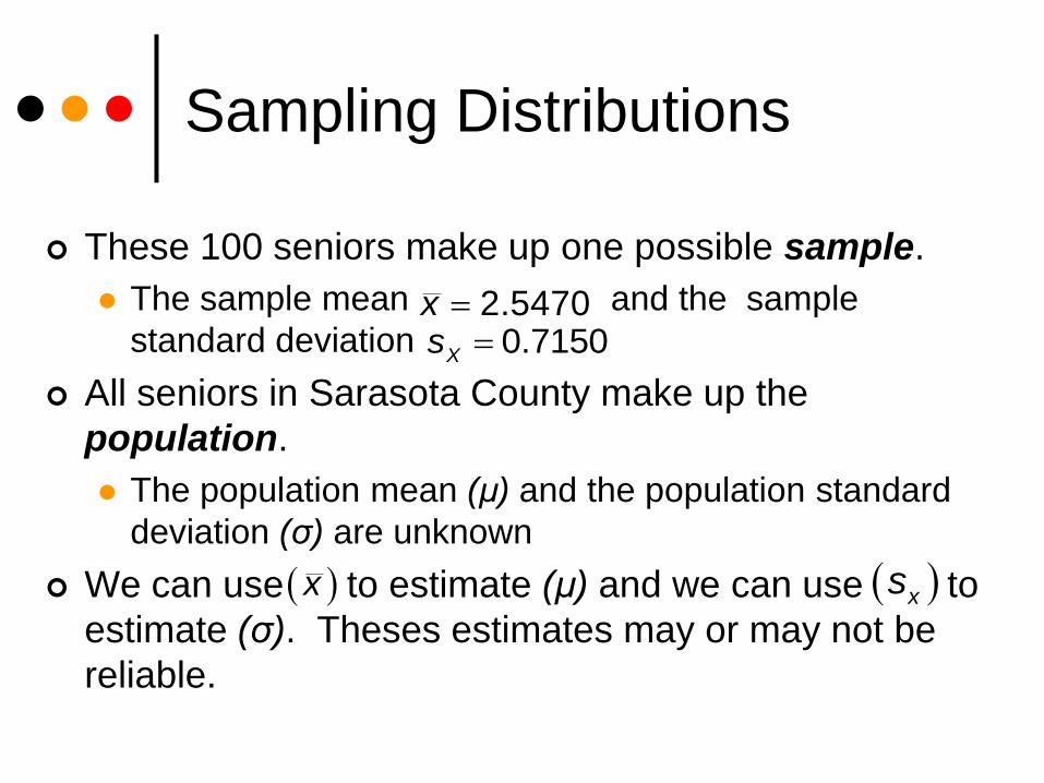
These 100 seniors make up one possible sample.
The sample mean and the sample
standard deviation
All seniors in Sarasota County make up the
population.
The population mean (μ) and the population standard
deviation (σ) are unknown
We can use to estimate (μ) and we can use to
estimate (σ). Theses estimates may or may not be
reliable.
2.5470x 0.7150Xs
x xs

Parameter and Statistics
A number that describes the population is
called a parameter.
Therefore, (μ) and (σ) are both parameters.
A parameter is usually represented by (p).
A number that is computed from a sample
is called a statistics.
Therefore, and are both statistics.
A statistic is usually represent by
x Xs
p̂

Sampling Variability
If I had chosen a different 100 seniors, then I would have a different sample, but it would still represent the same population.
A different sample almost always produce different results.
If I compare many different samples and the statistic is very similar in each one.
The sampling variability is low.
If I compare many different samples and the statistic is very different in each one.
The sampling variability is high.
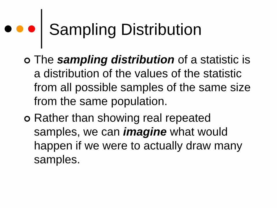
Sampling Distribution
The sampling distribution of a statistic is
a distribution of the values of the statistic
from all possible samples of the same size
from the same population.
Rather than showing real repeated
samples, we can imagine what would
happen if we were to actually draw many
samples.
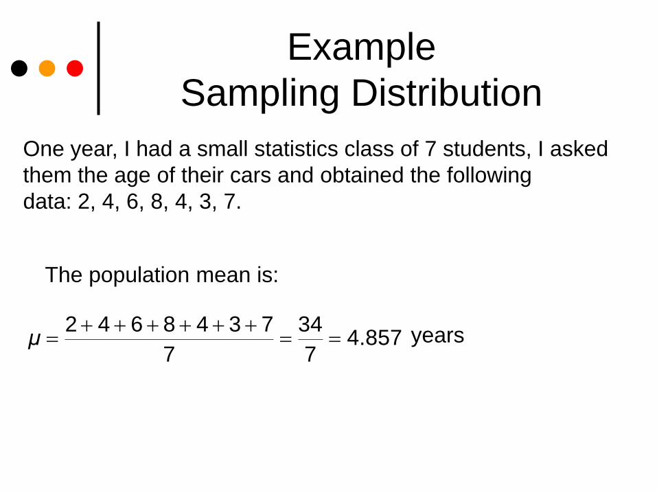
Example
Sampling Distribution
One year, I had a small statistics class of 7 students, I asked
them the age of their cars and obtained the following
data: 2, 4, 6, 8, 4, 3, 7.
The population mean is:
2 4 6 8 4 3 7 344.857
7 7μ
years

Example
Sampling Distribution
Construct a sampling distribution of the mean for sample
size n = 2.
There are total of 7 individuals in the population. We are
selecting them two at time without replacement. Therefore,
there are 7C2 = 21 samples of size n = 2.

Example
Sampling DistributionSample Sample Mean Sample Sample Mean Sample Sample Mean
2, 4 3 4, 8 6 6, 7 6.5
2, 6 4 4, 4 4 8, 4 6
2, 8 5 4, 3 3.5 8, 3 5.5
2, 4 3 4, 7 5.5 8, 7 7.5
2, 3 2.5 6, 8 7 4, 3 3.5
2, 7 4.5 6, 4 5 4, 7 5.5
4, 6 5 6, 3 4.5 3, 7 5
Mean of statistic values102
4.85721 21
x
x x x

Example
Sampling Distribution
0.00
0.05
0.10
0.15
0.20
Pro
bab
ilit
yty
2.5 3 3.5 4 4.5 5 5.5 6 6.5 7 7.5
Sample Means
Probability Distribution of the Sample Mean

Example
Sampling DistributionSample Distribution of the Sample Mean
Sample Mean Frequency Probability
2.5 1 1/21
3 2 2/21
3.5 2 2/21
4 2 2/21
4.5 2 2/21
5 4 4/21
5.5 3 3/21
6 2 2/21
6.5 1 1/21
6.5 1 1/21
7 1 1/21
7.5 1 1/21
What is the probability of
obtaining a sample mean
between 4 and 6 years,
inclusive – (4 6)?P x
13
(4 6) 0.61921
P x
If we took 10 random samples
of size 2 from this population,
about 6 of them would result
in sample means between 4
and 6 years inclusive.

Example – Page 493, #9.6
Use your calculator to replicate Exercise 9.5 as follows. The command
randbin(20,0.50) simulates tossing a coin 20 times. The output is the
number of heads in 20 tosses. The command randbin(20,0.50,10)/20
simulates 10 repetitions of tossing the coin 20 times and finding the
proportions of heads. Go into your statistics/List editor and place
your cursor on top of L1/list1. Execute the command
randbin(20,0.50,10)/20.
20,0.50,10)/20.

Example – Page 493, #9.6
A). Plot a histogram of the 10 values of p̂

Example – Page 493, #9.6
B). Increase the number of repetitions to 100. The
command should read randbin(20,0.50,100)/20.
Describe the shape of the distribution
The center is close to 0.50, and the shape is approximately normal

Example – Page 493, #9.6
C). Use PLOT 2 to be a boxplot. How close is the median
(in the boxplot) to the mean (balance point) of the
histogram?
The mean and median are extremely close.

Example – Page 493, #9.6
D). Note that we didn’t increase the sample size, only
the number of repetitions. Did the spread of the
distribution change? What would you change to
decrease the spread of the distribution?
The spread change very little. To decrease the
spread, I would increase the number of trials, n.
For example, randbin(50,0.50)

Describing
Sampling Distributions
Shape
Is the shape of the distribution symmetric or
approximately normal?
Center
Is the center of the distribution very close to the true
value?
Spread
Do the values of the sample have a large spread?
Outliers
Are there any deviations from the overall pattern?

Lesson 9-1, Part 2
Sampling Distribution

Unbiased Statistic
The statistic used to estimate a parameter is
unbiased if the mean of its sampling
distribution is equal to the true value of the
parameter being estimated.
Sample proportion is an unbiased
estimator of the population proportion (p).
Sample mean is an unbiased estimator of
the population mean (μ).
p̂
x

Variability of a Statistic
The variability of a statistic is described by
the spread of its sampling distribution.
This spread is determined by the sampling
design and size of the sample.
A statistics can be unbiased and still have
high variability. To avoid this, increase the
size of the sample.
Larger samples give smaller spread.

Example – Page 499, #9.8
The table below contains the results of simulating on a computer 100
repetitions of the drawing of an SRS of size 200 from a large lot of
ball bearings. Ten percent of the bearings in the lot do not conform
to the specifications. That is, p = 0.10 for this population. The numbers
in the table are the counts of nonconforming bearings in each sample
of 200.
17 23 18 27 15 17 18 13 16 18 20 15 18 16 21 17 18 19 16 23
20 18 18 17 19 13 27 22 23 26 17 13 16 14 24 22 16 21 24 21
30 24 17 14 16 16 17 24 21 16 17 23 18 23 22 24 23 23 20 19
20 18 20 25 16 24 24 24 15 22 22 16 28 15 22 9 19 16 19 19
25 24 20 15 21 25 24 19 19 20 28 18 17 17 25 17 17 18 19 18
Example – Page 499, #9.8
A). Make a table that shows how often each count occurs. For each
count in your table, give the corresponding value of sample
proportion . Then draw a histogram for the values
of the statistic .
ˆ / 200p count
p̂

Example – Page 499, #9.8
Count Count Count
9 9/200
= 0.045
1 18 18/200=
0.090
12 24 0.120 10
13 0.065 3 19 0.095 9 25 0.125 4
14 0.070 2 20 0.100 7 26 0.130 1
15 0.075 5 21 0.105 5 27 0.135 2
16 0.080 11 22 0.110 6 28 0.140 2
17 0.085 12 23 0.115 7 30 0.150 1
p p̂ p p̂ p p̂

Example – Page 499, #9.8
The histogram actually does not appear to have a normal shape. The
sampling distribution is quite normal in appearance, but even a sample of
size 100 does not necessarily show it.

Example – Page 499, #9.8
p̂The mean of is 0.0981
C). Find the mean of the 100 observations of . Mark the mean on your
histogram to show its center. Does the statistic appear to have a
large or small bias as an estimate of the population proportion p?
p̂p̂
The bias seems to be small

Example – Page 499, #9.8
D). The sampling distribution of is the distribution of the values of
from all possible samples of size 200 from this population. What
is the mean of this distribution?
p̂
p̂
The mean of the sampling distribution should be p = 0.10
p̂
E). If we repeatedly selected SRSs of size 1000 instead of 200 from
this same population, what would be the mean of the sampling
distribution of the sample proportion ? Would the spread be larger,
smaller, or about the same when compared with the spread of your
histogram in (a).
The mean would still be 0.10, but the spread would be smaller
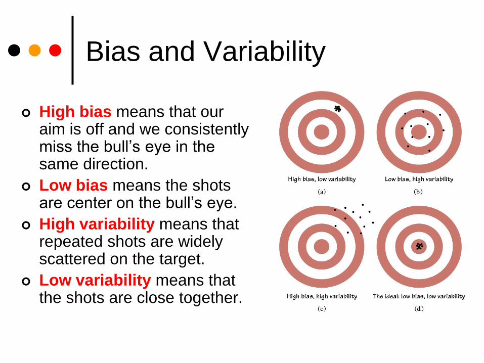
Bias and Variability
High bias means that our aim is off and we consistently miss the bull’s eye in the same direction.
Low bias means the shots are center on the bull’s eye.
High variability means that repeated shots are widely scattered on the target.
Low variability means that the shots are close together.

Example – Page 501, #9.10
Figure 9.10 shows histograms of four sampling distributions of
statistics intended to estimate the same parameter. Label each
distribution relative to the others as having large or small bias and
as having large or small variability.

Example – Page 501, #9.10
Large bias and large variability

Example – Page 501, #9.10
Small bias and small variability
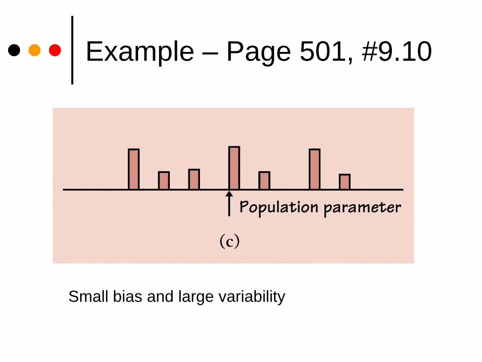
Example – Page 501, #9.10
Small bias and large variability

Example – Page 501, #9.10
Large bias and small variability
Lesson 9-2
Sample Proportions
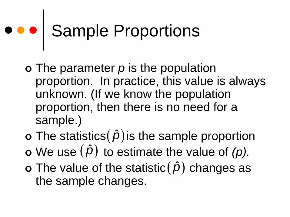
Sample Proportions
The parameter p is the population proportion. In practice, this value is always unknown. (If we know the population proportion, then there is no need for a sample.)
The statistics is the sample proportion
We use to estimate the value of (p).
The value of the statistic changes as the sample changes.
p̂
p̂
p̂

Sampling Distribution of
Sample Proportion
p̂
p̂
ˆx
pn
If our sample is an SRS of size n, then the following statements describe
the sampling distribution for
1. The shape is approximately normal.
ASSUMPTION: Sample size is sufficiently large
CONDITION: np 10 and n(1 – p) 10
2. Let be the proportion of the sample having that characteristic.
The mean of the sampling distribution is exactly p
Wherex is the count “success in a sample
n is the size of the sample

Sampling Distribution of
Sample Proportion
3. The standard deviation is
ASSUMPTION: Sample size is sufficiently large
CONDITION: The population is at least 10 times as large as the
sample.
(1 )x
p p pqs
n n

Summary
Select a large SRS from a population of which the proportion p are success.
The sampling distribution of the proportion of success in the sample
is approximately normal.
p̂

Sample Proportions
If we have categorical data, then we must use sample proportions to construct a sampling model.
Example – Suppose we want to know how many seniors in Florida plan to attend college. We want to now how many seniors answer, “Yes” to the question, “Do you plan to attend college?” These responses are categorical.
So p (our parameter) is the proportion of all seniors in Florida who plan to attend college
Let (our statistic) be the proportion of Florida students in an SRS of size 100 who plan to attend college.
To calculate the value of , we divide the number of “Yes” responses in our sample by the total number of students in the sample.
p̂
p̂

Sampling Model
If I graph the value of for all possible samples of
size 100, then I have constructed a sampling model.
What will the sample model look like?
It will be approximately normal. In fact, the larger my
sample size, the closer it will be a normal model.
So how large is large enough to ensure that the
sampling model is close normal?
Both np 10 and nq 10 in order for normal
approximations to be useful.
p̂

Sampling Model
The mean of sample model will equal the true
population
The standard deviation (if the population is
least 10 times as large as the sample) will be
pqσ
n

Example – Page 511, #9.20
The Gallup Poll asked a probability sample of 1785 adults whether they attended
church or synagogue during the past week. Suppose that 40% of the adult
population did attend. We would like to know the probability that SRS of size
1785 would come within plus or minus 3 percentage points of this true value.
A). If is the proportion of the sample who did attend church or
synagogue, what is the mean of the sampling distribution of ?
What is its standard deviation?
p̂
p̂
0.40μ p
0.40 1 0.40(1 )0.0116
1785
p pσ
n

Example – Page 511, #9.20
B). Explain why you can use the formula for the standard deviation of
in this setting (rule of thumb 1)p̂
0.40
1785
0.0116
μ p
n
σ
The population (U.S adults) is considerably larger than 10 times
the sample size

Example – Page 511, #9.20
C). Check that you can use the normal approximation for the
distribution of (rule of thumb 2).p̂0.40
1785
0.0116
μ p
n
σ
10 (1 ) 10np and n p
714 10 1071 10

Example – Page 511, #9.20
p̂
0.40
1785
0.0116
μ p
n
σ
D). Find the probability that takes a value between 0.37 and 0.43.
Will an SRS of size 1785 usually give a result within plus or
minus 3 percentage points of the true population proportion?
Explain.
p̂
ˆ(0.37 0.43) (0.37,0.43,.40,0.0116) 0.99P p normalcdf
Over 99% of all samples should give within ±3% of the
true population proportion
p̂

Example – Page 511, #9.22
Harley-Davidson motorcycles make up 14% of all the motorcycles in the
United States. You plan to interview an SRS of 500 motorcycles owners.
A) What is the approximate distribution of your sample who
own Harleys?
The distribution is approximately normal with mean
μ = p = 0.14
Standard deviation is
(1 ) 0.14(0.86)0.0155
500
p pσ
n

Example – Page 511, #9.22
B) How likely is your sample to contain 20% or more who own
Harley’s. Do a normal probability calculation to answer
this question.
μ = p = 0.14
σ = 0.0155ˆ( 0.20) 0.00005P p
5(0.20, 99,0.14,0.0155) 5.42 10 0.00005normalcdf E
20% or more Harley owners is unlikely

Example – Page 511, #9.22
C) How likely is your sample to contain 15% or more who own
Harley’s. Do a normal probability calculation to answer
this question.
μ = p = 0.14
σ = 0.0155ˆ( 0.15) 0.2594P p
(0.15, 99,0.14,0.0155) 0.2594normalcdf E
There is a fairly good chance of finding at least 15%
Harley owners.

Lesson 9-3, Part 1
Sample Means

Sample Means
If we have quantitative data, then we must use sample means to construct a sampling model.
Example – Suppose I randomly select 100 seniors in Florida and record each one’s GPA. I am interested in knowing the average GPA of a senior in Florida.
These 100 seniors make up one possible sample.• Sample mean is
• Sample standard deviation is
So p (our parameter) is the true mean GPA of a senior in Florida.
Let (our statistic) is the mean GPA of a senior in Florida in an SRS of size 100.
To calculate the value of , we find the mean our sample .
p̂
p̂
x xs
x
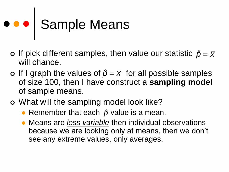
Sample Means
If pick different samples, then value our statistic will chance.
If I graph the values of for all possible samples of size 100, then I have construct a sampling modelof sample means.
What will the sampling model look like?
Remember that each value is a mean.
Means are less variable then individual observations because we are looking only at means, then we don’t see any extreme values, only averages.
p̂ x
p̂ x
p̂
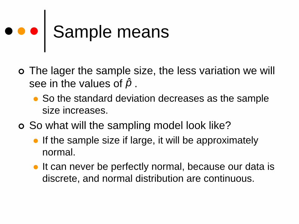
Sample means
The lager the sample size, the less variation we will
see in the values of .
So the standard deviation decreases as the sample
size increases.
So what will the sampling model look like?
If the sample size if large, it will be approximately
normal.
It can never be perfectly normal, because our data is
discrete, and normal distribution are continuous.
p̂

Sample Means
The mean of the sampling model of will
equal the true population mean
The standard deviation will be (if the
population is at least 10 times as large as
the sample)
x
σσ
n
x
xμ μ
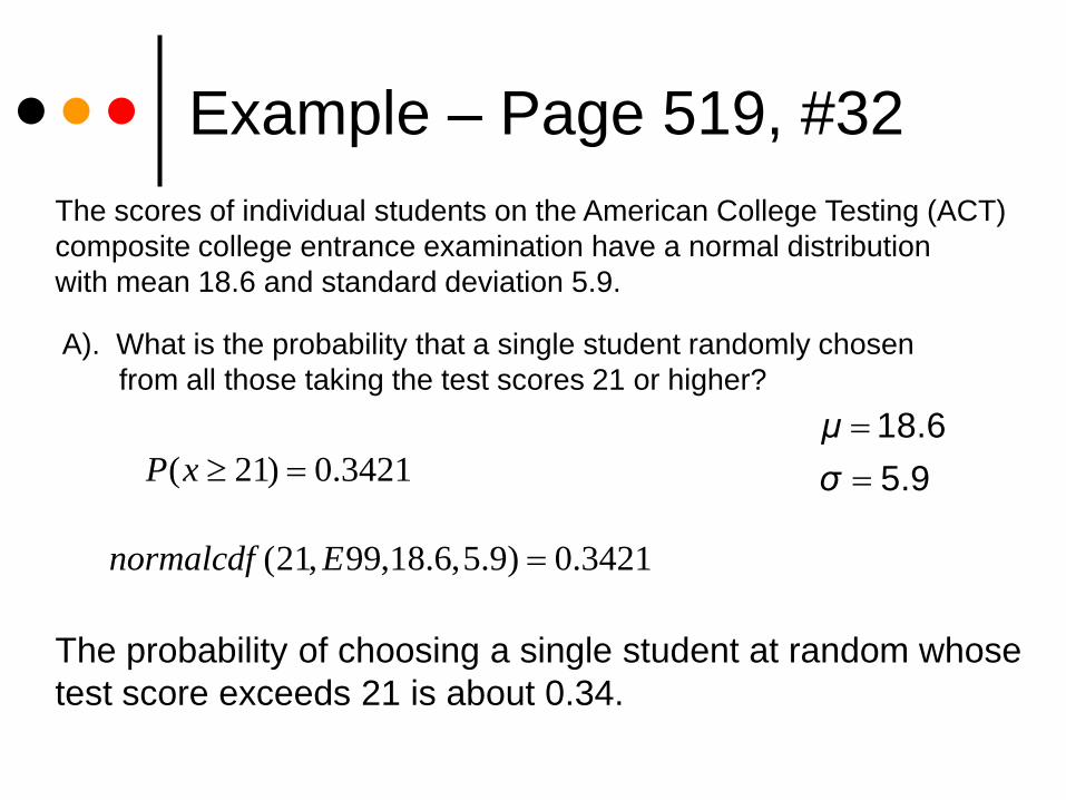
Example – Page 519, #32
The scores of individual students on the American College Testing (ACT)
composite college entrance examination have a normal distribution
with mean 18.6 and standard deviation 5.9.
A). What is the probability that a single student randomly chosen
from all those taking the test scores 21 or higher?
( 21) 0.3421 P x
(21, 99,18.6,5.9) 0.3421normalcdf E
18.6
5.9
μ
σ
The probability of choosing a single student at random whose
test score exceeds 21 is about 0.34.

Example – Page 519, #32
B). Know take an SRS of 50 students who took the test. What are the mean
and standard deviation of the average (sample mean) score for the
50 students? Do you results depend on the fact that individual scores
have a normal distribution?
18.6X 5.9 0.8344
50X
n
This result is independent of distribution shape.

Example – Page 519, #32
C). What is the probability that the mean score of these students is 21
or higher?
( 21) 0.0020 P x
(21, 99,18.6,0.8344) 0.0020normalcdf E
18.6
0.8344
x
x
μ μ
σ
It is very unlikely (less than 1% chance) that we would
draw an SRS of 50 students whose average score exceeds
21.

Example – Page 519, #9.34
A study of the health of teenagers plans to measure the blood
cholesterol level of an SRS of youth of ages 13 to 16 years. The
researchers will report the sample mean from their sample as the
estimate of the mean cholesterol level μ in this population.
A). Explain to someone who knows no statistics what it means to say
that x is “unbiased” estimator of μ.
If we choose many samples, the average of the x values
from these samples will be close μ.

Example – Page 519, #9.34
B). The sample result x is an unbiased estimator of the population
parameter μ no matter what the size SRS the study chooses.
Explain to someone you knows no statistics why a large sample
gives more trustworthy results than a small sample.
The larger sample will give more information, and therefore
more precise results; that is x is more likely to be close
to the true population.

Lesson 9-3, Part 2
Central Limit Theorem

Central Limit Theorem
For any population, regardless of
its shape, as the sample size
increases, the shape of the
distribution becomes more “normal”
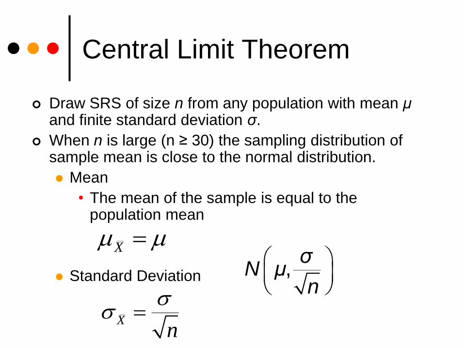
Central Limit Theorem
Draw SRS of size n from any population with mean μand finite standard deviation σ.
When n is large (n ≥ 30) the sampling distribution of sample mean is close to the normal distribution.
Mean
• The mean of the sample is equal to the population mean
Standard Deviation
X
Xn
,σ
N μn

Sampling Distribution of a
Sample Mean

Example – Page 525, #9.40
A company that owns and services a fleet of cars for its
sale force has found that the service lifetime of disc brake
pads varies from car to car according to a normal distribution
with mean μ = 55,000 miles and standard deviation σ = 4500
miles. The company installs a new brand of brake pads on
8 cars.
A). If the new brand has the same lifetime distribution as
the previous type, what is the distribution of the sample
mean lifetime for the 8 cars.
4500
55000, 55000,15918
N N
Example – Page 525, #9.40
B). The average life of the pads on these 8 cars turn out be
51,800 miles. What is the probability that the sample
mean lifetime is 51,800 miles or less if the lifetime
distribution is unchanged? (The company takes this
probability as evidence that the average lifetime of the
new brand of pads is less than 55,000 miles).
55000
4500
1591X
( 51800) 0.02215P x
( 99,51800,55000,1591) 0.02215normalcdf E

Example – Page 526, #9.42
Children in kindergarten are sometimes given the Ravin Progressive Matrices
Test (RPMT) to assess their readiness for learning. Experience at Southwark
Elementary School suggests that the RPMT scores for its kindergarten
pupils have mean 13.6 and standard deviation 3.1. The distribution is close
to normal. Mr. Lavin has 22 children in his kindergarten class this year. He
suspects that their RPMT scores will be unusually low because the test was
interrupted by a fire drill. To check this suspicion, he wants to find the level L
such that there is probability only 0.05 that the mean score of 22 children
falls below L when the usual Southwark distribution remains true. What is
the value of L?
L
0.05
13.6
3.10.05,13.6, 12.51322
invorm