Chapter 9

Scale space

Scale is one of the most important concepts in human vision. When we look at ascene, we instantaneously view its contents at multiple scale levels. For example,take a look at figure 9.1. This painting contains a wealth of objects ’living’ at a

wide range of scales, from small-scale objects such as the cracks in the pavement tolarge-scale structures such as the building in the background. Humans apparently arenot easily confused by the occurrence of multiple scales in a single scene, because wehave no trouble at all identifying what is building and what is not, despite the fact thatthe building consists of numerous details and components at lower scales.

Another vision phenomenon is that details (low-scale structures) simply seem to disap-pear if we move away from an object. For example, suppose you are facing the wallof a large brick building, close enough to distinguish individual bricks and the mortarbetween. If you move away from the building, the layers of mortar will disappear at acertain distance, giving the wall a uniform look. Instead of disappearing, details mayalso seem to merge under particular circumstances. For example, a row of shrubs mayseem to be a single structure when seen from a large enough distance.

Including the notion of scale into computer vision and image processing techniques isno trivial matter. In the previous chapters, almost all of the techniques presented fo-cused on small-scale image structures. The smallest scale in digital images is the scaleof the individual pixels (the inner scale of the image), and our spatial operators mostlyused discrete kernels with a size very close to this scale, such as 3 × 3 kernels, or con-tinuous kernels with a small support. In this chapter, we will examine a technique tocontrol the scale with which operators ’look’ at a digital image.

9.1 Scale space

The key to adjusting an operator to a certain scale seems to be altering the image res-olution. Put naively, we could re-sample a digital image at a low resolution to bring

248 Scale space

Figure 9.1 Canaletto’s San Marco square. An example of a scene with objects at multiplescales.

9.1 Scale space 249

large-scale object into the range of, e.g., our 3× 3 kernel. For an example, see figure 9.2,where we have decreased the resolution so that a 3 × 3 kernel operates on larger-scalestructures than in the original image. The resolution of an image can be decreased by

Figure 9.2 A 256× 256 image, and the same image re-sampled to a resolution of 25× 25 pixelsusing nearest neighbor interpolation. Using a 3 × 3 kernel on the right image now operateson structures of a much larger scale than in the original image. Notice that the re-samplingapparently introduces structures not present in the original. Consider for instance the shape andpatterning of the orca’s body as suggested by the low-resolution image, and compare it to theactual shape and pattern of the original.

merging the grey values of a block of pixels into the new grey value of a larger pixel.This merging can, e.g., be done by averaging grey values, by taking the center pixelvalue, or by taking the maximum, minimum, modal, nearest neighbor value, etc. Thistechnique of lowering the resolution to bring large-scale structures into ’kernel range’and remove small-scale structures, is a much-used and easy to implement technique;we will come back to this technique in section 9.3. It however suffers from some prob-lems that are inherent to the very blocky nature of representing low-resolution imagesby square pixels, the most serious of which is often the occurrence of spurious resolution:the apparent creation of structures that are not present in the original image. Spuriousresolution can be seen in figure 9.2.

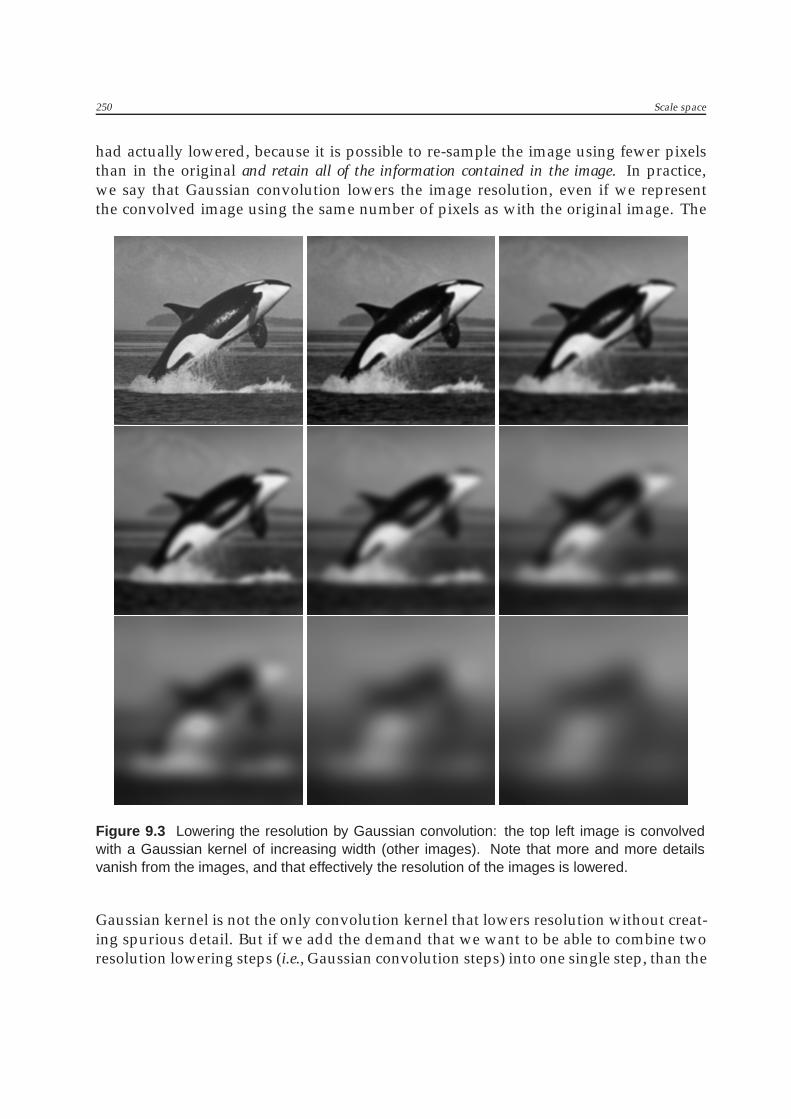
We are looking for an operation that lowers resolution but does not introduce new de-tails into the image; that avoids spurious resolution. We have already come across suchan operation many times: convolution with a Gaussian. Figure 9.3 shows example ofresolution lowering by convolution with a Gaussian. Note that we use the term res-olution here in a more abstract, intrinsic sense than before: upon convolution with aGaussian, the actual number of pixels used in an image need not change, so the resolu-tion in terms of the number of pixels used does not change. However, after convolutionthe smallest recognizable detail in the image has become larger, and it that sense the res-olution is lower than before. We can also say that the intrinsic resolution of the image

250 Scale space

had actually lowered, because it is possible to re-sample the image using fewer pixelsthan in the original and retain all of the information contained in the image. In practice,we say that Gaussian convolution lowers the image resolution, even if we representthe convolved image using the same number of pixels as with the original image. The

Figure 9.3 Lowering the resolution by Gaussian convolution: the top left image is convolvedwith a Gaussian kernel of increasing width (other images). Note that more and more detailsvanish from the images, and that effectively the resolution of the images is lowered.

Gaussian kernel is not the only convolution kernel that lowers resolution without creat-ing spurious detail. But if we add the demand that we want to be able to combine tworesolution lowering steps (i.e., Gaussian convolution steps) into one single step, than the

9.1 Scale space 251

Gaussian kernel is the only possible kernel. This demand makes intuitive sense: sup-pose we wish to lower the resolution by some amount a, and after that by some amountb, then it should be possible to do this in one step, lowering the resolution by an amounta+ b.

The stack of images as seen in figure 9.3 is called a Gaussian scale space. We denote theGaussian scale space of an image f(x, y) by fσ(x, y), where σ is the standard deviationof the Gaussian kernel gσ(x, y) used in the convolution:

fσ(x, y) = gσ(x, y) ∗ f(x, y).

The Gaussian scale space is called a one-parameter extension of the original image, be-cause we now have three parameters (x, y, and σ) instead of two (x and y). The resolu-tion parameter σ is called the scale of the image fσ(x, y)

The Gaussian scale space can be viewed as a stack of images, where the original imageis at the bottom of the stack (f0(x, y) = f(x, y)), and the image resolution gets lower aswe rise in the stack, see figure 9.4.

With the Gaussian scale space, we now have a construct that allows us to ‘select’ animage at a certain level of resolution. The next question is how to use this construct sothat we are able to apply an operator to an image only at a certain scale level σ1. Ingeneral, it is not very effective to apply such an operator directly to the image fσ1(x, y).The reason for this is that –even though the intrinsic resolution of the image fσ1(x, y)is lower than the resolution of the original1– we still use the same number of pixels asin the original image to represent the image at scale σ1. Subsampling the image so thatwe use less pixels than in the original image can partially solve this problem. However,there is a method that solves this problem in a mathematically sound way when theoperator we wish to apply is a differential operator. This method is covered in the nextsection.

9.1.1 Scaled differential operators

Given an image fσ1 ; an image at scale σ1: fσ1 = gσ1 ∗ f . Suppose we wish to computethe derivative of the image fσ1 to x, i.e., the derivative of f to x at scale σ1. Consider thisequation:

∂fσ1

∂x=

∂

∂x(gσ1 ∗ f)

F−→ 2πiu(Gσ1F ) = (2πiuGσ1)F

F−1

−→ ∂gσ1

∂x∗ f.

1Assuming that σ1 = 0.

252 Scale space

x

y

σ

Figure 9.4 The Gaussian scale space of an image. The original image rests at the bottom ofthe stack (σ = 0), and the scale σ increases as we rise in the stack.

Here, F and F−1 denote the Fourier and inverse Fourier transform. In this equation, wehave used the properties that convolution in the spatial domain becomes multiplicationin the Fourier domain, and that taking the derivative to x in the spatial domain becomesmultiplication with 2πiu in the Fourier domain. Cutting out the middle part of theequation gives us:

∂fσ1

∂x=∂gσ1

∂x∗ f.

The left term shows us what we wish to compute: the scaled (σ1) derivative of f to x.The right term shows us how we can compute this in a well-posed mathematical way:

9.1 Scale space 253

we compute the derivative of the Gaussian kernel and convolve the result with our origi-nal image f . This way, we avoid having to compute the derivative of the digital imagef , which is an ill-posed problem. Instead, we only need to compute the derivative of aGaussian, which is a well-posed problem, because the Gaussian function is a differen-tiable function. If we compute the scaled derivative entirely in the Fourier domain, onlymultiplications are needed.

Figure 9.5 shows some examples of scaled x derivatives of an image.

Figure 9.5 Scaled x derivatives of the top-left (256×256) image, respectively with σ = 1, 2, 4, 8, 16pixels.

This example with the scaled x derivative of an image can be generalized to all spatialderivatives: to compute a scaled spatial derivative, we need only compute the appro-priate derivative of the Gaussian kernel (with standard deviation σ equal to the desiredscale), and convolve the result with the original image. So, if we denote partial deriva-tives by subscripts x or y, for example:

fσ1,x = gσ1,x ∗ ffσ1,y = gσ1,y ∗ ffσ1,xy = gσ1,xy ∗ ffσ1,xxx = gσ1,xxx ∗ fetc.

254 Scale space

9.1.2 Scaled differential features

Many image features, such as edges, ridges, corners, etc. can be detected using differen-tial operators. In many cases, the detection of interesting features benefits from tuningthe differential operators to the appropriate scale.

Invariants. In many applications, features like the x or y derivative of an image arenot by themselves interesting features. More interesting are so-called invariant features–also concisely denoted simply by invariants– i.e., features that are insensitive to somekind of transformation. For example, the x derivative of an image is not invariant underrotation, because the following two operations give different results: (1) computing thex derivative, and (2) rotating the image, computing the x derivative, then rotating the

result back. The gradient norm (√f 2x(a) + f 2

y (a), in a point a), however, is invariantunder rotation because the two operations: (1) computing the gradient norm, and (2)rotating the image, computing the gradient norm, then rotating the result back, yieldsthe same result. All of the features treated in the below are invariant under translationsand rotations.

Gradient-based coordinate system. The gradient vector plays an important role in thedetection of many different types of features. It is therefore often convenient to abandonthe usual (x, y) Cartesian coordinate frame, and replace it with a local coordinate framebased on the gradient vector w and its right-handed normal vector v. This local (v, w)frame is sometimes called a gauge or Frenet frame. In formulas, the v and w vectors canbe written as

w =

(fxfy

)and v =

(fy−fx

).

Figure 9.6 shows an example of an image where we have drawn several (v, w) frames.Note that the gradient vector w always points ‘uphill’, and that the normal vector v isalways in the direction of an isophote (i.e., a curve of equal image intensity). It mayat first seem strange to use a coordinate system that may point a different way in eachpixel, but it is in fact very convenient when we consider features invariant under ro-tations (and translations). This is because when we rotate an image, the (v, w) framesrotate with it, because the v and w vectors are based on the local image structure. Thismeans that all derivatives computed in the v or w directions are also invariant. Putdifferently, the (v, w) frame captures some of the intrinsic differential structure of theimage, independent of how you have chosen your (x, y) coordinate system.

As we denote the derivative of an image in the x direction by fx, we adopt a similarnotation for derivatives in the v or w direction. For example, the first derivative of f inthe w direction is denoted by fw, the second by fww, etc.

9.1 Scale space 255

vv

vv

w

w

w

w

Figure 9.6 The (v,w) coordinate frame drawn at four random points in an image. The w vectorequals the local gradient.

For the actual computation of expressions such as fw, fvw, fwww, etc. we usually need torewrite them in a Cartesian form (using fx, fy, fxy, etc. which we know how to compute).The intermezzo below shows how this ‘translation’ can be achieved.

Intermezzo∗

Derivatives of a function f specified using v andw subscripting can be translated toa Cartesian form (using only partial derivatives to x and y) by using the definitionof the directional derivative:

The derivative of f in the direction of a certain row vector a is defined as

fa =1||a|| (a · ∇)f,

where ∇ is the Nabla vector defined by ∇ =

(∂∂x∂∂y

), and the dot (·) denotes the

inner product.

For example, if we take a to be the vector (1, 2), then fa equals:

fa = 1√5

((1 2) ·

(∂∂x∂∂y

))f = 1√

5

(∂∂x + 2 ∂

∂y

)f = 1√

5

(∂f∂x + 2∂f∂y

)=

= 1√5(fx + 2fy).

256 Scale space

Note that this directional derivative definition is consistent with the definition ofthe Cartesian derivatives. For example, fx, i.e., the directional derivative of f in thedirection (1, 0):

fx =11

((1 0) ·

(∂∂x∂∂y

))f =

(∂

∂x

)f =

∂f

∂x

We can now compute the derivatives fv and fw:2

fw =1√

f2x + f2

y

((fx fy) ·

(∂∂x∂∂y

))f =

fxfx + fyfy√f2x + f2

y

=√f2x + f2

y .

fv =1√

f2x + f2

y

((fy − fx) ·

(∂∂x∂∂y

))f =

(fyfx − fxfy)√f2x + f2

y

= 0.

Perhaps not surprisingly, the derivative fw equals the gradient magnitude, and fvis zero. The latter is because v is in the direction of the local isophote, i.e., the curvewhere f does not change value.

Higher order directional derivatives can be computed using the following exten-sion:

f a . . . a︸ ︷︷ ︸n times

=1||a||n (a · ∇)nf.

For example, the Cartesian form of fvv is

fvv = 1||v||2

((fy −fx) ·

(∂∂x∂∂y

))2

f

= 1f2

x+f2y

(fy

∂∂x − fx ∂

∂y

)2f

= 1f2

x+f2y

(f2y∂2

∂x2 − 2fxfy ∂2

∂x∂y + f2x∂2

∂y2

)f

= f2y fxx−2fxfyfxy+f2

xfyy

f2x+f2

y.

2Note that we compute the directional derivative along a straight line; the derivative along the v or wvector. We do not compute the derivative along the integral curves of the local v or w vectors. The latterform gives distinctly different results. Also, note that in our expressions we take the derivatives fx andfy to be constants, so the differential operators affect only f itself.

9.1 Scale space 257

Edges. In chapter 5 we introduced the gradient ∇f(b) in a certain point b as a vectorthat always points in the most uphill direction if we view the image as an intensitylandscape. The gradient is also perpendicular to the local isophote. The norm of the

gradient ||∇f(b)|| =√f 2x(b) + f 2

y (b) is a measure for the edgeness in b.

Another edgeness measure is based on the second derivatives of f : the Laplacian, Δf =fxx + fyy. In this case, edges are assumed to be located at the zero crossings of themeasure. Both the gradient norm and the Laplacian are computed using first or secondorder partial derivatives of the image f . We can now compute these derivatives in ascaled way, using a certain scale σ. The figures 9.7 and 9.8 show some examples ofscaled edgeness images. Note the results of high-scale operators in noisy environmentsin figure 9.8.

Ridges. If we view an image as an intensity landscape, one of the most characteristicfeatures are the landscape’s ridges. The definition of a ridge in terms of image deriva-tives still sparks some debate, apparently because different people usually have differ-ent ideas as to what exactly the ridges in an image are3. In fact, many different defini-tions can be found, each defining similar yet different ridge-like structures in an image.

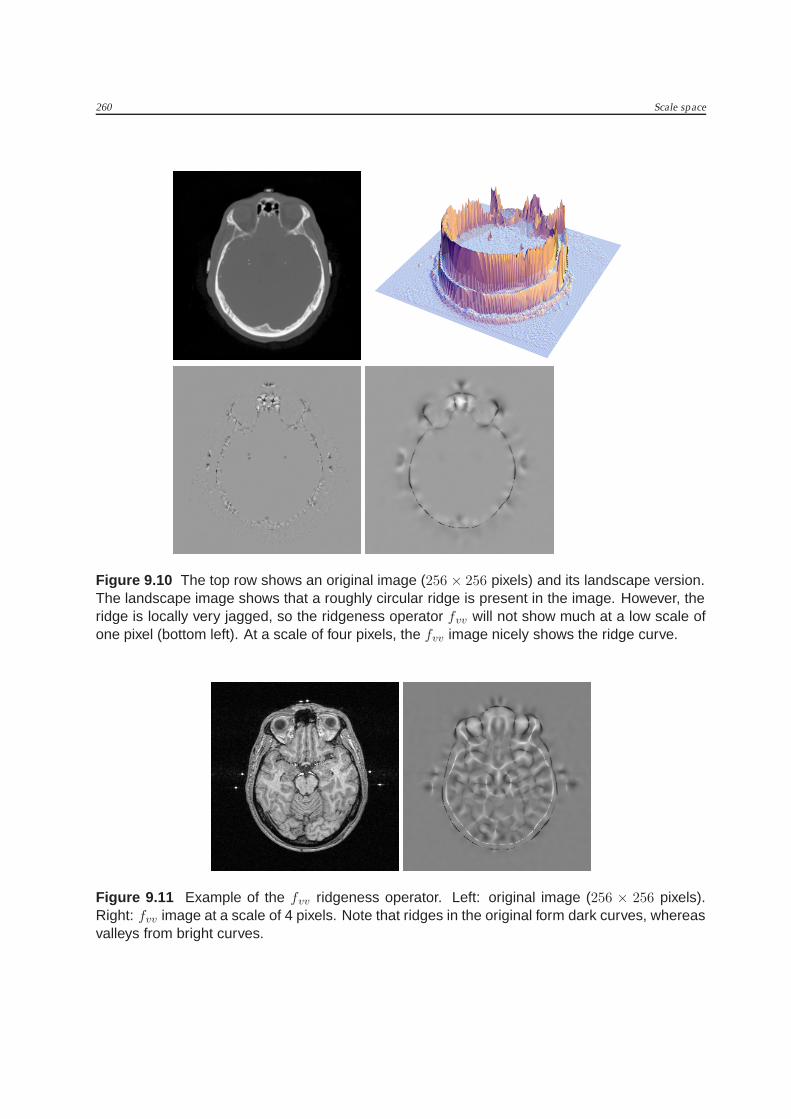
One ridge definition that appeals to the intuition is one based on the (v, w) gradient-based coordinate frame: figure 9.9 shows part of an image depicted as an intensitylandscape. At a ridge point (1), and two other randomly chosen points, we have drawnthe gradient vector w. If we plot the grey values around the ridge point in the v and thew direction (left two plots of the four), then only the v direction plot shows a concaveprofile. This is because the v direction is the direction crossing the ridge. The sameplots at a non-ridge point do not show any significant concavity. This is the basis ofour definition for ridgeness: the concavity of the grey-value profile in the v direction.Since the second derivative is a measure for concavity, our ridgeness measure is simplyfvv . For the Cartesian form of this measure see the intermezzo above. Figure 9.10 showssome examples of fvv images at different scales. The measure not only detects ridges(low fvv values), but also ‘valleys’ (high fvv values), see figure 9.11. Figure 9.9 can alsobe used to define another ridgeness operator: In any non-ridge point, it can be observedthat the local gradient is pointing roughly toward the ridge. In a ridge point, the gra-dient is directed along the ridge. This means that if we travel from the left point to theright one via the ridge point, the gradient will turn swiftly as we cross the ridge. Thegradient turning speed when traveling in the v direction through an image may there-fore be another ridgeness operator. We can measure this turning speed as follows: theorientation of the gradient can be characterized by an angle θ with the positive x-axis,i.e., θ = arctan(fy/fx). Its rate of change (turning speed of the gradient) equals its firstderivative, here taken in the v direction. This results in the expression 1

||v||(v ·∇)θ, which

3Unfortunately, this holds true to some extent for most types of image features.

258 Scale space

Figure 9.7 Edgeness images at different scales. Top row: original, 256×256 image. Middle row:gradient norm at scales 1, 4 and 8 pixels. Bottom row: Laplacian images at scales 1, 4, and 8pixels. Note that details vanish from the edgeness images as the scale increases. However, thelocalization certainty decreases with increasing scale; the ‘resolution’ of the edge is lowered.

9.1 Scale space 259

Figure 9.8 Gradient norm edgeness images of a 256 × 256 artificial image (top left), and of thesame image with added noise (bottom left). The middle and right column show the edgenessimages at scales of 1 and 16 pixels respectively. Note that only the 16 pixel scale performs wellin the noisy image.

vv

v

www

1 2

f f

ff

vv

w w

1 2

Figure 9.9 The grey-value profiles in the v and w (gradient) directions at a ridge point (1), anda non-ridge point (2). Note that only the v-profile in the ridge point is markedly concave.

260 Scale space

Figure 9.10 The top row shows an original image (256 × 256 pixels) and its landscape version.The landscape image shows that a roughly circular ridge is present in the image. However, theridge is locally very jagged, so the ridgeness operator fvv will not show much at a low scale ofone pixel (bottom left). At a scale of four pixels, the fvv image nicely shows the ridge curve.

Figure 9.11 Example of the fvv ridgeness operator. Left: original image (256 × 256 pixels).Right: fvv image at a scale of 4 pixels. Note that ridges in the original form dark curves, whereasvalleys from bright curves.

9.1 Scale space 261

can be worked out in the same manner as before:

1

||v||(v · ∇)θ =2fxfyfxy − f 2

y fxx − f 2xfyy

(f 2x + f 2

y )32

.

It turns out this expression is very similar to the fvv ridgeness operator. In fact, it equals−fvv

fw, so the only difference is the minus sign and a normalization with respect to the

gradient magnitude fw. This latter aspect makes that the fvv

fwresponds more in low-

contrast image areas than fvv . The measure fvv

fwis also known in literature as the isophote

curvature. Figure 9.12 shows some examples of −fvv

fwimages.

Figure 9.12 Examples of the fvv

fwridgeness operator. Left column: original 256 × 256 images.

Right column: fvv

fwimages at a scale of four pixels. Note that the operator also responds in low

contrast image areas.

Other differential geometric structures. It would be beyond the scope of this book totreat in detail other differential geometric structures. It is however illustrative to showsome examples of other operators, to give some idea of their capabilities in relation toimage processing. Table 9.1 lists a number of operators (all invariant under rotation andtranslation). Note that names for expressions (such as cornerness) are descriptive at best,and should not be taken in too literal a sense. The figures 9.13 through 9.16 show someexample images.

262 Scale space

Name (expression) Cartesian formEdgeness, fw

√f 2x + f 2

y

Ridgeness, fvvf2

y fxx−2fxfyfxy+f2xfyy

f2x+f2

y

Isophote curvature; ridgeness, −fvv

fw−f2

y fxx−2fxfyfxy+f2xfyy

(f2x+f2

y )32

Cornerness, fvvf 2w f 2

y fxx − 2fxfyfxy + f 2xfyy

Flowline curvature, −fvw

fw

fxfy(fyy−fxx)+fxy(f2x−f2

y )

(f2x+f2

y )32

Isophote density, fww (or fww

fw) fxxf2

x+2fxyfxfy+fyyf2y

f2x+f2

y

Umbilicity 2(fxxfyy−f2xy)

f2xx+2f2

xy+f2yy

Unflatness f 2xx + 2f 2

xy + f 2yy

Checkerboard detector −(fxxxxfyyyy − 4fxxxyfxyyy + 3fxxyyfxxyy)3 +

27(−fxxxy(fxxxyfyyyy − fxyyyfxxyy) +fxxyy(fxxxyfxyyy− fxxyyfxxyy)+ fxxxx(fxxyyfyyyy−fxyyyfxyyy))

2

Table 9.1 Examples of differential invariants.

9.2 Scale space and diffusion∗

The physical processes of diffusion and heat conduction offer a new view of scale space.At a first glance, these processes and scale space appear to be unrelated, but considerfigure 9.17. Suppose the left graph represents the temperature as a function of lengthalong a metal rod. After a certain amount of time, the temperature distribution willhave evolved to the state represented by the right graph. As you may have guessedfrom the shape of the graphs, the right graph is nothing but the left graph convolvedwith a Gaussian. The temperature distribution at any time after the initial state can becomputed by convolving the initial distribution with a Gaussian, where the width σis directly related to the time a certain state occurs. Figure 9.18 shows some evolutionstates. The collection of all evolution states equals the scale space of the original state.

The physical process of heat conduction is usually modeled by the following partialdifferential equation:

ft = α2fxx,

where f = f(x, t) represents the temperature at position x at time t, and α is a material-dependent constant. This equation is known as the heat or diffusion equation (it can beused as a model for either process). It models how the temperature distribution evolves:the change in time (ft) depends only on the current temperature distribution, and some

9.2 Scale space and diffusion∗ 263

Figure 9.13 Top row: original (256× 256) image, and two cornerness images at scales of 1 and16 pixels. Bottom row: same original image, with added noise, and the cornerness images atthe same two scales. Note that only the large scale can cope with the (small scale) noise.

nifty modeling that we won’t report here shows that the change in time is proportionalto the second spatial derivative of f , as the equation shows. The two-dimensional formof this equation is

ft = α2Δf,

where Δf equals the Laplacian Δf = ∇ · (∇f) = fxx + fyy. If we assume the function fhas an infinite spatial domain, it can be shown that a solution f(x, τ) at a certain time τcan be found by convolving the initial state f(x, 0) with a Gaussian function with widthσ =√

2α2t.

In terms of images, this means that we can regard a scaled image fσ(x, y) as the solutionof the heat equation at a time related to σ, where the original image f = f0(x, y) is theinitial ‘temperature distribution’, if we think of a grey value as a temperature.

The heat conduction model can be extended to include some common phenomena. Forexample, in practice we may need to model the heat conduction in situations where

264 Scale space

Figure 9.14 Top row: original noisy (256 × 256) image of part of a checkerboard, and twocheckerboard detector images at scales of 1 and 16 pixels. Bottom row: 256 × 256 CT imageand checkerboard detector images at scales of 1 and 8 pixels

Figure 9.15 fww isophote density images at scales of 1, 4, and 8 pixels of the CT image in theprevious figure.

9.2 Scale space and diffusion∗ 265

Figure 9.16 Umbilicity images at scales of 1, 4, and 8 pixels of the CT image used in theprevious figures. The umbilicity operator distinguishes elliptical (positive value) and hyperbolic(negative value) areas of the image intensity landscape.

Figure 9.17 Scale space and the physical process of heat conduction. Left: temperature as afunction of length of a metal rod. Right: the same function, after some time has elapsed andnormal heat conduction has taken place. These functions are related to scale space: the rightgraph is in fact the left graph convolved with a Gaussian.

Figure 9.18 Some temperature evolution states of the function in the previous figure (plottedvertically above each other for clarity). The space of the temperature evolution equals the scalespace of the original state.

266 Scale space

different materials –with different heat conduction speeds– are involved. An extendedheat equation that can handle heat conduction that changes in space and time is

ft = ∇ · (c∇f),

where c = c(x, y, t) is a measure for the local heat conduction. If c is very small at acertain location, then almost no heat will flow across that location when time passes.This is where the analogy of scale space vs. heat conduction becomes interesting: it isoften a drawback of scale space is that edges of objects become very blurred (diffused!)at high scales. Sometimes, it is useful if we could somehow preserve the edges of objectsat a scale σ or larger. We can do this by making c(x, y, t) small if (x, y) is located at anedge. To determine if (x, y) is located at an edge, we can use the gradient magnitude fw(computed at the right scale) as an edgeness measure. A suitable formula for c (one ofmany, really) is

c =1

1 +(fw

K

)2 ,

where K is a positive constant. The heat equation with this c substituted is known asthe Perona-Malik equation. Applying this equation to an image creates a totally differentscale space than when c = 1, as in the ’normal’ scale space.

We can create other scale spaces by modifying the c function so that diffusion aroundsome type of geometrical structures (edges, ridges, etc. ) is encouraged or discouraged.The generating equations can then, e.g., be ft = fw, ft = fvv , ft = f

1/3vv f

2/3w , etc. , to respec-

tively encourage diffusion at edges, at ridges (diffuse in the center of objects rather thanat the edges), and at corners4. Figure 9.19 shows some examples. Figure 9.20 shows anoise reduction application.

While computing a scaled image in the Gaussian scale space is relatively easy –it re-quires only convolution of the original image with a Gaussian– images in the other scalespaces mentioned cannot usually be computed directly, because the necessary convolu-tion kernel is different in each location of the image. In practice, scaled images are com-puted by letting the underlying differential equation evolve to the desired scale (time),using a numerical method (such as Euler’s method) to approximate the solution of theequation.

4Evolution of an image according to these three equations are also known as normal flow, Euclideanshortening flow, and affine shortening flow respectively.

9.3 The resolution pyramid 267

Figure 9.19 Top row: original image and two scaled versions from a scale space generated bythe equation ft = fvv. Bottom row: three scaled images from a scale space generated by thePerona-Malik equation.

9.3 The resolution pyramid

At the start of this chapter, we mentioned a simple method for lowering the resolutionof an image: divide the image in regular blocks of pixels (say 2 × 2 pixels each), andmerge the pixels in each block to a single new pixel. This merging can be done by,e.g., averaging the pixel values, taking (e.g.) the top-left pixel value, or taking the max-imum or minimum pixel value. We can apply the same operation to the results, andagain to its results, etc. creating a series of images –each image with a lower resolutionthan the image before it– called a resolution pyramid. Figure 9.21 shows an example.

This method of resolution lowering lacks most of the useful mathematical propertiesthat scale space has, and it is not straightforward how to lower the resolution by a factorthat is not integer. Nevertheless, the resolution pyramid is extremely useful in its ownright in many different applications. This is because an image in the pyramid retainsmuch of the global structure of the original image (exactly how much depending onthe pyramid level), while taking less memory bytes to store. In general, processing ofa pyramid image is significantly faster than processing the original image. A common

268 Scale space

way to employ the pyramid is to do fast and coarse processing on the top level image(the lowest resolution image), and use its results to guide processing at the level belowit, continuing until the original image (the bottom level of the pyramid) is reached. Foran example, we show the use of a pyramid in an image registration application.

Example: image registration using a multiresolution pyramid

Suppose we have two 256 × 256 images that need to be brought into registrationby rotation and translation of one of the two:

We want the registration error to be no more than one pixel size anywhere in theimage. The straightforward ’brute force’ approach to find the correct registrationis to examine all possible transformations, computing a suitable registration mea-sure in each case, in finally picking the transformation for which the measure ismaximum. Unfortunately, this approach results in over 60 million configurationsto check, and so is not usually a feasible approach to take.

A better approach is to build a (e.g.) four level pyramid:

9.3 The resolution pyramid 269

The top level images have a 32 × 32 resolution, and the number of possible trans-formations that are no more than one pixel length apart is now low enough foreach to be examined separately. Each examination in itself is also much faster thanexamining the original, because the number of pixels is reduced by a factor of 64.

The best transformation found at the top pyramid level will be too coarse to be veryaccurate at the next pyramid level, but it can function as a suitable starting positionat this level. At this level, we again examine a number of transformations and pickout the best one, but keep the number of transformations down by examining onlya suitable range of transformations around the starting position. In this fashion,we continue down the pyramid until we reach the original image, where we canfind the optimal transformation by examining only a relatively small number oftransformations around the starting position.

The possibility of a coarse-to-fine strategy such as the one described above is not onlyan asset of the resolution pyramid, but also of any scale space. The implementation anduse of the strategy is most straightforward in the case of the resolution pyramid. Thepyramid, however, lacks many of the useful mathematical properties of scale space thatenable a more robust approach using scale space techniques instead of the pyramid inmany applications.

270 Scale space

Figure 9.20 Scale space generated from the top left image using the equation f t = fvv. A zoomof the orginal and top right image shows that a moderate scaling of an image removes noisewithout touching essential image structures much.

9.3 The resolution pyramid 271

Figure 9.21 Example of a resolution pyramid. The original 256 × 256 image is on the left. Thenext image is formed by averaging each block of 4 pixels into a single pixel, forming a 128 × 128image. Each following image is formed in the same manner; the final image has a resolution of8× 8 pixels.

272 Scale space