Chapter 9

Optimal Control and InverseProblems

The purpose of Optimal Control is to influence the behavior of a dynamicalsystem in order to achieve a desired goal. Optimal control has a large va-riety of applications where the dynamics can be controlled optimally, suchas aerospace, aeronautics, chemical plants, mechanical systems, finance andeconomics, but also to solve inverse problems where the goal is to determineinput data in an equation from its solution values. An important applica-tion we will study in several settings is to determine the ”data” in di!erentialequations models using optimally controlled reconstructions of measured ”so-lution” values.

Inverse problems are typically harder to solve numerically than forwardproblems since they are often ill-posed (in contrast to forward problems),where ill-posed is the opposite of well-posed and a problem is defined to bewell-posed if the following three properties holds

(1) there is a solution,

(2) the solution is unique, and

(3) the solution depends continuously on the data.

It is clear that a solution that does not depend continuously on its data isdi"cult to approximate accurately, since a tiny perturbation of the data (ei-ther as measurement error and/or as numerical approximation error) may

99

give a large change in the solution. Therefore, the ill-posedness of inverseand optimal control problems means that they need to be somewhat mod-ified to be solved: we call this to regularize the problem. Optimal controltheory is suited to handle many inverse problems for di!erential equations,since we may formulate the objective – for instance to optimally reconstructmeasured data or to find an optimal design – with the di!erential equationas a constraint. This chapter explains:

• the reason to regularize inverse problems in an optimal control setting,

• a method how to regularize the control problem, and

• in what sense the regularized problem approximates the original prob-lem.

To give some intuition on optimal control and to introduce some basic con-cepts let us consider a hydro-power generator in a river. Suppose that we arethe owners of such a generator, and that our goal is to maximise our profit byselling electricity in some local electricity market. This market will o!er usbuying prices at di!erent hours, so one decision we have to make is when andhow much electricity to generate. To make this decision may not be a trivialtask, since besides economic considerations, we also have to meet technicalconstraints. For instance, the power generated is related to the amount ofwater in the reservoir, the turbined flow and other variables. Moreover, if wewant a plan for a period longer than just a few days the water inflow to thelake may not be precisely known, making the problem stochastic.

We can state our problem in optimal control terms as the maximization ofan objective function, the expected profit from selling electricity power duringa given period, with respect to control functions, like the hourly turbinedflow. Observe that the turbined flow is positive and smaller than a givenmaximum value, so it is natural to have a set of feasible controls, namelythe set of those controls we can use in practice. In addition, our dynamicalsystem evolves according to a given law, also called the dynamics, which herecomes from a mass balance in the dam’s lake. This law tells us how the statevariable, the amount of water in the lake, evolves with time according to thecontrol we give. Since the volume in the lake cannot be negative, there existadditional constraints, known as state constraints, that have to be fulfilledin the optimal control problem.

After introducing the formulation of an optimal control problem the nextstep is to find its solution. As we shall see, the optimal control is closely

100

related with the solution of a nonlinear partial di!erential equation, knownas the Hamilton-Jacobi-Bellman equation. To derive the Hamilton-Jacobi-Bellman equation we shall use the dynamic programming principle, whichrelates the solution of a given optimal control problem with solutions tosimpler problems.

9.1 The Determinstic Optimal Control Set-ting

A mathematical setting for optimally controlling the solution to a determin-istic ordinary di!erential equation

Xs = f(Xs, !s) t < s < T

X t = x(9.1)

is to minimize

inf!!A

! " T

t

h(Xs, !s) ds + g(XT )#

(9.2)

for given cost functions h : Rd ! [t, T ] " R and g : Rd " R and a given setof control functions A = {! : [t, T ]" A} and flux f : Rd !A" Rd. Here Ais a given compact subset of some Rm.

9.1.1 Examples of Optimal Control

Example 9.1 (Optimal control of spacecraft) To steer a spacecraft withminimal fuel consumption to an astronomical body may use the gravitationalforce from other bodies. The dynamics is determined by the classical New-ton’s laws with forces depending on the gravity on the spacecraft and its rocketforces, which is the control cf. [?].

Example 9.2 (Inverse problem: Parameter reconstruction) The op-tion values can be used to detemine the volatility function implicitly. The ob-jective in the optimal control formulation is then to find a volatility functionthat yields option prices that deviate as little as possible from the measuredoption prices. The dynamics is the Black-Scholes equation with the volatilityfunction to be determined, that is the dynamics is a determinstic partial dif-ferential equation and the volatility is the control function, see Section 9.2.1.

101

This is a typical inverse problem: it is called inverse because in the standardview of the Black-Scholes equation relating the option values and the volaility,the option price is the unknown and the volatility is the data; while here theformulation is reversed with option prices as data and volatility as unknownin the same Black-Scholes equation.

Example 9.3 (Inverse problem: Weather prediction) The incompress-ible Navier-Stokes equations are used to forecast weather. The standard math-ematical setting of this equation is an initial value problem with unknownvelocity and pressure to be determined from the initial data: in weather pre-diction one can use measured velocity and pressure not only at a single initialinstance but data given over a whole time history. An optimal control formu-lation of the weather prediction is to find the first initial data (the control)matching the time history of measured velocity and pressure with the Navier-Stokes dynamics as constraint. Such an optimal control setting improves theaccuracy and makes longer forecast possible as compared to the classical ini-tial value problem, see [?], [?]. This is an inverse problem since the velocityand pressure are used to determine the ”initial data”.

Example 9.4 (Merton’s stochastic portfolio problem) A basic problemin finance is to choose how much to invest in stocks and in bonds to maximizea final utility function. The dynamics of the portfolio value is then stochas-tic and the objective is to maximize an expected value of a certain (utility)function of the portfolio value, see section 9.3.1.

Example 9.5 (Euler-Lagrange equation) The shape of a soap bubble be-tween two wires can be deterimined as the surface that minimizes the area.Here the whole surface is the control function and its graph solves the Euler-Lagrange equation...

Example 9.6 (Inverse problem: Optimal design) An example of opti-mal design is to construct an electrical conductor to minimize the power lossby placing a given amount of conductor in a given domain, see Section9.2.1.This is an inverse problem since the conductivity is determined from the elec-tric potential in an equation where the standard setting is to determine theelectric potential from the given conductivity.

102

9.1.2 Approximation of Optimal Control

Optimal control problems can be solved by the Lagrange principle or dynamicprogramming. The dynamic programming approach uses the value function,

defined by u(x, t) := inf!!A

! $ T

t h(Xs, !s) ds + g(XT )#

for the ordinary dif-

ferential equation (9.1) with Xt # Rd, and leads to solution of a non linearHamilton-Jacobi-Bellman partial di!erential equation

"tu(x, t) + min!!A

%f(x, !) · "xu(x, t) + h(x, !)

&

' () *H("xu(x,t),x)

= 0, t < T,

u(·, T ) = g,

(9.3)

in (x, t) # Rd ! R+. The Lagrange principle (which seeks a minimum of thecost with the dynamics as a constraint) leads to the solution of a Hamiltoniansystem of ordinary di!erential equations, which are the characteristics of theHamilton-Jacobi-Bellman equation

X "t = f(X t, !t), X0 given,

$#"ti = "xif(X t, !t) · #t + h(X t, !t), #T = g"(XT ),

!t # argmina!A

!#t · f(X t, a) + h(X t, a)

#,

(9.4)

based on the Pontryagin Principle. The next sections explain these twomethods.

The non linear Hamilton-Jacobi partial di!erential approach has the the-oretical advantage of well established theory and that a global minimum isfound; its fundamental drawback is that it cannot be used computationallyin high dimension d % 1, since the computational work increases exponen-tially with the dimension d. The Lagrange principle has the computationaladvantage that high dimensional problems, d % 1, can often be solved andits drawback is that in practice only local minima can be found compu-tationally, often with some additional error introduced by a regularizationmethod. Another drawback with the Lagrange principle is that it (so far)has no e"cient implementation in the natural stochastic setting with adaptedMarkov controls, while the Hamilton-Jacobi PDE approach directly extendsto such stochastic controls, see Section 9.3; as a consequence computationsof stochastic controls is basically limited to low dimensional problems.

103

9.1.3 Motivation of the Lagrange formulation

Let us first review the Lagrange multiplier method to minimize a functionsubject to a constraint minx!A, y=g(x) F (x, y). Assume F : Rd ! Rn " R is adi!erentiable function. The goal is to find the minimum minx!A F (x, g(x))for a given di!erentiable function g : Rd " Rn and a compact set A & Rd.This problem leads to the usual necessary condition for an interior minimum

d

dxF

%x, g(x)

&= "xF

%x, g(x)

&+ "yF

%x, g(x)

&"xg(x) = 0. (9.5)

An alternative method to find the solution is to introduce the Lagrangianfunction L(#, y, x) := F (x, y) + # ·

%y $ g(x)

&with the Lagrange multiplier

# # Rn and choose # appropriately to write the necessary condition for aninterior minimum

0 = "#L(#, y, x) = y $ g(x),

0 = "yL(#, y, x) = "yF (x, y) + #,

0 = "xL(#, y, x) = "xF (x, y)$ # · "xg(x).

Note that the first equation is precisely the constraint. The second equationdetermines the multiplier to be # = $"yF (x, y). The third equation yieldsfor this multiplier "xL($"yF (x, y), y, x) = d

dxF%x, g(x)

&, that is the multi-

plier is chosen precisely so that the partial derivative with respect to x ofthe Lagrangian is the total derivative of the objective function F

%x, g(x)

&

to be minimized. This Lagrange principle is often practical to use whenthe constraint is given implicitly, e.g. as g(x, y) = 0 with a di!erentiableg : Rd ! Rn " Rn; then the condition det "yg(x, y) '= 0 in the implicitfunction theorem implies that the function y(x) is well defined and satis-fies g

%x, y(x)

&= 0 and "xy = $"yg(x, y)#1"xg(x, y), so that the Lagrange

multiplier method works.The Lagrange principle for the optimal control problem (9.1) -(9.2), to

minimize the cost with the dynamics as a constraint, leads to the Lagrangian

L(#, X, !) := g(XT ) +

" T

0

h(Xs, !s) ds +

" T

0

#s ·%f(Xs, !s)$ X

&ds (9.6)

with a Lagrange multiplier function # : [0, T ] " Rd. Di!erentiability ofthe Lagrangian leads to the necessary conditions for a constrained interior

104

minimum

"#L(X, #, !) = 0,

"XL(X, #, !) = 0,

"!L(X, #, !) = 0.

(9.7)

Our next step is to verify that the two first equations above are the same asthe two first in (9.4) and that the last equation is implied by the strongerPontryagin principle in the last equation in (9.4). We will later use theHamilton-Jacobi equation in the dynamic programming approach to verifythe Pontryagin principle.

The first equation. Choose a real valued continuous function v : [0, T ]"Rd and define the function L : R " R by L($) := L(X, # + $v,!). Thenthe first of the three equations means precisely that L"(0) = d

d$L(X, # +$v,!)|$=0 = 0, which implies that

0 =

" T

0

vs ·%f(Xs, !s)$ Xs

&ds

for any continuous function v. If we assume that f(Xs, !s)$Xs is continuouswe obtain f(Xs, !s)$ Xs = 0: since if %(s) := f(Xs, !s)$ Xs '= 0 for somes there is an interval where % is either positive or negative; by choosing v tobe zero outside this interval we conclude that % is zero everywhere and wehave derived the first equation in (9.4).

The second equation. The next equation dd$L(X + $v,#, !)|$=0 = 0 needs

v0 = 0 by the initial condition on X0 and leads by integration by parts to

0 =

" T

0

#s ·%"Xif(Xs, !s)vs

i $ vs&

+ "Xih(Xs, !s)vsi ds + "Xig(XT )vT

i

=

" T

0

#s · "Xif(Xs, !s)vsi + # · vs + "Xih(Xs, !s)vs

i ds

+ #0 · v0'()*=0

$%#T $ "Xg(XT )

&· vT

=

" T

0

%"Xf $(Xs, !s)#s + #s + "Xh(Xs, !s)

&· vs ds

$%#T $ "Xg(XT )

&· vT ,

using the summation convention aibi :=+

i aibi. Choose now the functionv to be zero outside an interior interval where possibly "Xf $(Xs, !s)#s +

105

#s + "Xh(Xs, !s) is non zero, so that in particular vT = 0. We see thenthat in fact "Xf $(Xs, !s)#s + #s + "Xh(Xs, !s) must be zero (as for the firstequation) and we obtain the second equation in (9.4). Since the integral inthe right hand side vanishes, varying vT shows that the final condition forthe Lagrange multiplier #T $ "Xg(XT ) = 0 also holds.

The third equation. The third equation in (9.7) implies as above that forany function v(t) compactly supported in A

0 =

" T

0

#s · "!f(Xs, !s)v + "!h(Xs, !s)v ds

which yields#s · "!f(Xs, !s) + "!h(Xs, !s) = 0 (9.8)

in the interior ! # A $ "A minimum point (X, #, !). The last equation in(9.4) is a stronger condition: it says that ! is a minimizer of #s · f(Xs, a) +h(Xs, a) = 0 with respect to a # A, which clearly implies (9.8) for interiorpoints ! # A$ "A. To derive the Pontryagin principle we will use dynamicprogramming and the Hamilton-Jacobi-Bellman equation which is the sub-ject of the next section.

9.1.4 Dynamic Programming and the Hamilton-Jacobi-Bellman Equation

The dynamic programming view to solve optimal control problems is based onthe idea to track the optimal solution backwards: at the final time the valuefunction is given u(x, T ) = g(x) and then, recursively for small time stepbackwards, find the optimal control to go from each point (x, t) on the timelevel t to the time level t+#t with the value function u(·, t+#t) , see Figure9.1. Assume for simplicity first that h ( 0 then any path X : [t, t+#t]" Rd

starting in X t = x will satisfy

u(x, t) = inf!:[t,t+!t]%A

u(X t+!t, t + #t),

so that if u is di!erentiable

du(X t, t) =%"tu(X t, t) + "xu(X t, t) · f(X t, !t)

&dt ) 0, (9.9)

since a path from (x, t) with value u(x, t) can lead only to values u(X t+!t, t+#t) which are not smaller than u(x, t). If also the infimum is attained, then

106

an optimal path X t$ exists, with control !t

$, and satisfies

du(X t$, t) =

%"tu(X t

$, t) + "xu(X t$, t) · f(X t

$, !t$)

&dt = 0. (9.10)

The combination of (9.9) and (9.10) implies that

"tu(x, t) + min!!A

%"xu(x, t) · f(x, !)

&= 0 t < T

u(·, T ) = g,

which is the Hamilton-Jacobi-Bellman equation in the special case h ( 0.

r\-I-i dty i"'

I - |

\ /

/L--

i t' t

,b i15 _

+

K-. rof4l , r i

i

ks**&

t * v,.t:Ay

f . ^i;r - fi'Uvu vrt4

J 'J

k^

eq*1

"- l"ti r.1

1

^ v/ , '

_-d

#;:I

i

f,, )

'tiu+-

1#

I

l i

r,

r4'.

- --t---),"1

'', /

/ \

1n'J' t

Y,

ril t

z {n1

Oy b u,,4 puirrt

Figure 9.1: Illustration of dynamics programming.

The case with h non zero follows similarly by noting that now

0 = inf!:[t,t+!t]%A

! " t+!t

t

h(Xs, !s) ds + u(X t+!t, t + #t)$ u(x, t)#, (9.11)

which for di!erentiable u implies the Hamilton-Jacobi-Bellman equation (9.3)

0 = inf!!A

%h(x, !) + "tu(x, t) + "xu(x, t) · f(x, !)

&

= "tu(x, t) + min!!A

%"xu(x, t) · f(x, !) + h(x, !)

&

' () *=:H

%"xu(x,t),x

&t < T,

g = u(·, T ).

Note that this derivation did not assume that an optimal path is attained,but that u is di!erentiable which in general is not true. There is fortunatelya complete theory for non di!erentiable solutions to Hamilton-Jacobi equa-tions, with its basics presented in Section (9.1.6). First we shall relate theLagrange multiplier method with the Pontryagin principle to the Hamilton-Jacobi-Bellman equation using charateristics.

107

9.1.5 Characteristics and the Pontryagin Principle

The following theorem shows that the characteristics of the Hamilton-Jacobiequation is a Hamiltonian system.

Theorem 9.7 Assume u # C2, H # C1 and

X t = "#H%#t, X t

&

with #t := "xu(X t, t). Then the characteristics (X t, #t) satisfy the Hamilto-nian system

X t = "#H(#t, X t)

#t = $"XH(#t, X t).(9.12)

Proof. The goal is to verify that the construction of X t implies that #has the dynamics (9.12). The definition X t = "#H(#t, X t) implies by x-di!erentiation of the Hamilton-Jacobi equation along the path (X t, t)

0 = "x"tu(X t, t) + "#H%"xu(X t, t), X t

&"x"xu(X t, t) + "xH

%"xu(X t, t), X t

&

=d

dt"xu(X t, t) + "xH

%"xu(X t, t), X t

&

which by the definition #t := "Xu(X t, t) is precisely #t + "xH(#t, X t) = 0.!

The next step is to relate the characteristics X t, #t to the solution of theLagrange principle (9.4). But note first that the Hamiltonian H in general isnot di!erentiable, even if f and h are very regular: for instance X = f(X t)and h(x, !) = x! implies for A = [$1, 1] that the Hamiltonian becomesH(#, x) = #f(x)$ |x| which is only Lipschitz continuous, that is |H(#, x)$H(#, y)| * K|x$y| with the Lipschitz constant K = 1++# ·"xf(·)+& in thiscase. In fact if f and h are bounded di!erentiable functions the Hamiltonianwill always be Lipschitz continuous satisfying |H(#, x)$H(&, y)| * K(|#$&| + |x$ y|) for some constant K, see Exercise ??.

Theorem 9.8 Assume that f, h are x-di!erentiable in (x, !$) and a control!$ is optimal for a point (x, #), i.e.

# · f(x, !$) + h(x, !$) = H(#, x),

108

and suppose also that H is di!erentiable in the point or that !$ is unique.Then

f(x, !$) = "#H(#, x),

# · "xif(x, !$) + "xih(x, !$) = "xiH(#, x).(9.13)

Proof. We have for any w, v # Rd

H(# + w, x + v)$H(#, x) * (# + w) · f(x + v,!$) + h(x + v, !$)

$ # · f(x, !$)$ h(x, !$)

= w · f(x, !$) +d,

i=1

(# · "xif + "xih)vi + o(|v| + |w|)

which implies (9.13) by choosing w and v in all directions.!This Theorem shows that the Hamiltonian system (9.12) is the same as

the system (9.4), given by the Lagrange principle using the optimal control!$ with the Pontryagin principle

# · f(x, !$) + h(x, !$) = inf!!A

%# · f(x, !) + h(x, !)

&=: H(#, x).

If !$ is not unique (i.e not a single point) the proof shows that (9.13) stillholds for the optimal controls, so that "#H and "xH become set valued. Weconclude that non unique local controls !$ is the phenomenon that makes theHamiltonian non di!erentiable in certain points. In particular a di!erentiableHamiltonian gives unique optimal control fluxes "#H and "xH, even if !$ isnot a single point. If the Hamiltonian can be explicitly formulated, it istherefore often practical to use the Hamiltonain system formulation with thevariables X and #, avoiding the control variable.

Clearly, the Hamiltonian needs to be di!erentiable for the Hamiltoniansystem to make sense; in fact its flux ("#H,$"xH) must be Lipschitz continu-ous to give well posedness. On the other hand we shall see that the Hamilton-Jacobi-Bellman formulation, based on dynamic programming, leads to nondi!erentiable value functions u, so that classical solutions lack well posedness.The mathematical setting for optimal control therefore seemed somewhattroublesome both on the Hamilton-Jacobi PDE level and on the HamiltonODE level. In the 1980’s the situation changed: Crandall-Lions-Evans [?] for-mulated a complete well posedness theory for generalized so called viscositysolutions to Hamilton-Jacobi partial di!erential equations, allowing Lipschitz

109

continuous Hamiltonians. The theory of viscosity solutions for Hamilton-Jacobi-Bellman partial di!erential equations provides good theoretical foun-dation also for non smooth controls. In particular this mathematical theoryremoves one of Pontryagin’s two reasons1, but not the other, to favor theODE approach (9.4) and (9.12): the mathematical theory of viscosity so-lutions handles elegantly the inherent non smoothness in control problems;analogous theoretical convergence results for an ODE approach was devel-oped later based on the so called minmax solutions, see [?]; we will use analternative ODE method to solve optimal control problems numerically basedon regularized Hamiltonians, where we approximate the Hamiltonian with atwo times di!erentiable Hamiltonian, see Section 9.2.

Before we formulate the generalized solutions, we show that classical so-lutions only exist for short time in general.

Example 9.9 The Hamilton-Jacobi equation

"tu$1

2("xu)2 = 0

has the characteristics

X t = $#t

#t = 0,

which implies X t = constant. If the initial data u(·, T ) is a concave function(e.g. a smooth version of $|x|) characteristics X will collide, see Figure 9.2.We can understand this precisely by studying blow-up of the derivative w of"xu =: v; since v satisfies

"tv $1

2"x(v

2)' () *

v"xv

= 0

1citation from chapter one in [?] “This equation of Bellman’s yields an approach tothe solution of the optimal control problem which is closely connected with, but di!erentfrom, the approach described in this book (see Chapter 9). It is worth mentioning thatthe assumption regarding the continuous di!erentiability of the functional (9.8) [(??) inthis paper] is not fulfilled in even the simplest cases, so that Bellman’s arguments yield agood heuristic method rather than a mathematical solution of the problem. The maximumprinciple, apart from its sound mathematical basis, also has the advantage that it leadsto a system of ordinary di!erential equations, whereas Bellman’s approach requires thesolution of a partial di!erential equation.”

110

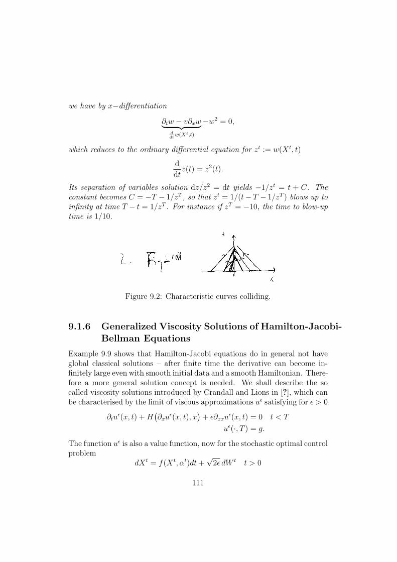
we have by x$di!erentiation

"tw $ v"xw' () *ddt w(Xt,t)

$w2 = 0,

which reduces to the ordinary di!erential equation for zt := w(X t, t)

d

dtz(t) = z2(t).

Its separation of variables solution dz/z2 = dt yields $1/zt = t + C. Theconstant becomes C = $T $ 1/zT , so that zt = 1/(t$ T $ 1/zT ) blows up toinfinity at time T $ t = 1/zT . For instance if zT = $10, the time to blow-uptime is 1/10.

r\-I-i dty i"'

I - |

\ /

/L--

i t' t

,b i15 _

+

K-. rof4l , r i

i

ks**&

t * v,.t:Ay

f . ^i;r - fi'Uvu vrt4

J 'J

k^

eq*1

"- l"ti r.1

1

^ v/ , '

_-d

#;:I

i

f,, )

'tiu+-

1#

I

l i

r,

r4'.

- --t---),"1

'', /

/ \

1n'J' t

Y,

ril t

z {n1

Oy b u,,4 puirrt

Figure 9.2: Characteristic curves colliding.

9.1.6 Generalized Viscosity Solutions of Hamilton-Jacobi-Bellman Equations

Example 9.9 shows that Hamilton-Jacobi equations do in general not haveglobal classical solutions – after finite time the derivative can become in-finitely large even with smooth initial data and a smooth Hamiltonian. There-fore a more general solution concept is needed. We shall describe the socalled viscosity solutions introduced by Crandall and Lions in [?], which canbe characterised by the limit of viscous approximations u$ satisfying for $ > 0

"tu$(x, t) + H

%"xu

$(x, t), x&

+ $"xxu$(x, t) = 0 t < T

u$(·, T ) = g.

The function u$ is also a value function, now for the stochastic optimal controlproblem

dX t = f(X t, !t)dt +,

2$ dW t t > 0

111

with the objective to minimize min! E[g(XT )+$ T

0 h(X t, !t)dt | X0given] overadapted controls ! : [0, T ]" A, where W : [0,-)" Rd is the d-dimensionalWiener process with independent components. Here adapted controls meansthat !t does not use values of W s for s > t. Section 9.3 shows that the valuefunction for this optimal control problem solves the second order Hamilton-Jacobi equation, that is u$(x, t) = min! E[g(XT ) +

$ T

0 h(X t, !t) dt | X t = x].

Theorem 9.10 (Crandall-Lions) Assume f, h and g are Lipschitz con-tinuous and bounded, then the limit lim$%0+ u$ exists. This limit is called theviscosity solution of the Hamilton-Jacobi equation

"tu(x, t) + H%"xu(x, t), x

&= 0 t < T

u(·, T ) = g.(9.14)

There are several equivalent ways to describe the viscosity solution di-rectly without using viscous or stochastic approximations. We shall use theone based on sub and super di!erentials presented first in [?]. To simplifythe notation introduce first the space-time coordinate y = (x, t), the space-time gradient p = (px, pt) # Rd+1 (related to ("xu(y), "tu(y))) and write theHamilton-Jacobi operator F (p, x) := pt +H(px, x). For a bounded uniformlycontinuous function v : Rd ! [0, T ] " R define for each space-time point yits sub di!erential set

D#v(y) = {p # Rd+1 : lim infz%0

|z|#1%v(y + z)$ v(y)$ p · z

&) 0}

and its super di!erential set

D+v(y) = {p # Rd+1 : lim supz%0

|z|#1%v(y + z)$ v(y)$ p · z

&* 0}.

These two sets always exist (one may be empty), see Example 9.11; theydegenerate to a single point, the space-time gradient of v, precisely if v isdi!erentiable, that is when

D#v(y) = D+v(y) = {p}./ v(y + z)$ v(y)$ p · z = o(z).

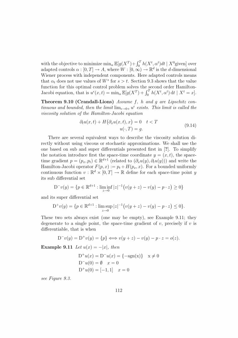
Example 9.11 Let u(x) = $|x|, then

D+u(x) = D#u(x) = {$sgn(x)} x '= 0

D#u(0) = 0 x = 0

D+u(0) = [$1, 1] x = 0

see Figure 9.3.

112

Definition 9.12 (Viscosity solution) A bounded uniformly continuous func-tion u is a viscosity solution to (9.14) if u(·, T ) = g and

F (p, x) ) 0 for all p # D+u(x, t)

andF (p, x) * 0 for all p # D#u(x, t).

Theorem 9.13 The first variation of the value function is in the superdif-ferential.

Proof. Consider an optimal path X$, starting in y = (x, t), with control!$. We define the first variation, (#t, & t) # Rd ! R, of the value functionalong this path, with respect to perturbations in the initial point y: let Xy

be a path starting from a point y = (x, t), close to y, using the control !$;the di!erentiability of the flux f and the cost h shows that

#ti = lim

z%0z#1

% " T

t

h(X tx+zei

, !t$)$ h(X t

x, !t$) dt + g(XT

x+zei)$ g(XT

x )&

(9.15)

and

$#t$ = "Xf(X t

$, !t$)#

t$ + "Xh(X t

$, !t$) t < t < T,

#T = g"(XT$ ),

where ei is the ith unit basis vector in Rd. The definition of the value functionshows that

$h(X t$, !

t$) =

du

dt(X t

$, t) = #t · f(X t$, !

t$) + &t

so that&t = $#t · f(X t

$, !t$)$ h(X t

$, !t$).

r\-I-i dty i"'

I - |

\ /

/L--

i t' t

,b i15 _

+

K-. rof4l , r i

i

ks**&

t * v,.t:Ay

f . ^i;r - fi'Uvu vrt4

J 'J

k^

eq*1

"- l"ti r.1

1

^ v/ , '

_-d

#;:I

i

f,, )

'tiu+-

1#

I

l i

r,

r4'.

- --t---),"1

'', /

/ \

1n'J' t

Y,

ril t

z {n1

Oy b u,,4 puirrt

Figure 9.3: Illustration of the sub and superdi!erential sets for $|x|.

113

Since the value function is the minimum possible cost, we have by (9.15)

lim sups%0+

s#1!u%y + s(y $ y)

&$ u(y)

#

* lim sups%0+

s#1! " T

t

h(X ty+s(y#y), !

t$) dt + g(XT

y+s(y#y))

$" T

t

h(X ty, !

t$) dt + g(XT

y )#

=!#t$,$

%#t$ · f(X t

$, !t$) + h(X t

$, !t$)

&#· (y $ y),

which means precisely that the first variation is in the superdi!erential. !

Theorem 9.14 The value function is semi-concave, that is for any point(x, t) either the value function is di!erentiable or the sub di!erential is empty(i.e. D#u(x, t) = 0 and D+u(x, t) is non empty).

Proof. Assume that the subdi!erential D#u(y) has at least two elementsp# and p+ (we will show that this leads to a contradiction). Then u is largeror equal to the wedge like function

u(y) ) u(y) + max%p# · (y $ y), p+ · (y $ y)

&, (9.16)

see Figure 9.4. The definition of the value function shows that the rightderivative satisfies

lim sups%0+

s#1!u%y + s(y $ y)

&$ u(y)

#* (#, &) · (y $ y) (9.17)

where (#, &) is the first variation (in x and t) of u around the optimal pathstarting in y. The wedge bound (9.16) implies

lim sups%0+

s#1!u%y + s(y $ y)

&$ u(y)

#) max

%p# · (y $ y), p+ · (y $ y)

&,

but the value function cannot be both below a (#, &)-half plane (9.17) andabove such wedge function, see Figure 9.5. Therefore the subdi!erentialcan contain at most one point: either the subdi!erential is empty or thereis precisely one point p in the subdi!erential and in this case we see thatthe the first variation coincides with this point (#, &) = p, that is the valuefunction is di!erentiable !

114

Theorem 9.15 The value function is a viscosity solution.

Proof. We have seen in Section 9.1.4 that for the points where the valuefunction is di!erentiable it satisfies the Hamilton-Jacobi-Bellman equation.Theorem 9.14 shows that the value function u is semi-concave. Therefore,by Definition 9.12, it is enough to verify that p # D+u(x, t) implies pt +H(px, x) ) 0. Assume for simplicity that h ( 0. Then the definition of thesuperdi!erential, for an optimal control !$ # A along an optimal path X t,and dynamic programming show that there is a p # D+u(x, t) that

pt + H(px, x) = p ·%f(x, !$), 1

&

) lim sup!t%0+

u(X t+!t, t + #t)$ u(X t, t)

#t= 0.

This means that any optimal control yields a super di!erential point p sat-isfying pt + H(px, x) ) 0. To finish the proof we note that any point in thesuper di!erential set can for some s # [0, 1] be written as a convex combi-nation sp1 + (1 $ s)p2 of two points p1 and p2 in the super di!erential thatcorrespond to optimal controls. Since H is concave in p (see Exercise 9.18)there holds

sp1t + (1$ s)p2

t + H%sp1

x + (1$ s)p2x, x

&

) s%p1

t + H(p1x, x)

&+ (1$ s)

%p2

t + H(p2x, x)

&

) 0

which shows that u is a viscosity solution. The general case with non zero his similar as in (9.11). !Theorem 9.16 Bounded uniformly continuous viscosity solutions are unique.

The standard uniqueness proof uses a special somewhat complex doubling ofvariables technique, see [?] inspired by Kruzkov. The maximum norm stabil-ity of semi-concave viscosity solutions in Section 9.1.7 also implies uniqueness.

r\-I-i dty i"'

I - |

\ /

/L--

i t' t

,b i15 _

+

K-. rof4l , r i

i

ks**&

t * v,.t:Ay

f . ^i;r - fi'Uvu vrt4

J 'J

k^

eq*1

"- l"ti r.1

1

^ v/ , '

_-d

#;:I

i

f,, )

'tiu+-

1#

I

l i

r,

r4'.

- --t---),"1

'', /

/ \

1n'J' t

Y,

ril t

z {n1

Oy b u,,4 puirrt

Figure 9.4: Characteristic curves colliding.

115

Example 9.17 Note that if we do not use that the subdi!erential is emptythe same technique as above works to verify that points p in the subdi!erential,generated by optimal paths, satisfy pt + H(px, x) * 0.

The Pontryagin Principle for Generalized Solutions

Assume that X$ and !$ is an optimal control solution. Let

$#t$ = "Xf(X t

$, !t$)#

t$ + "Xh(X t

$, !t$) t < T,

#T$ = g"(XT

$ ).

The proof of Theorem 9.13 shows first that!#t$,$

%#t$·f(X t

$, !t$)+h(X t

$, !t$)

&#

is the first variation in x and t of the value function at the point (X t, t) andconcludes then that the first variation is in the superdi!erential, that is

!#t$,$

%#t$ · f(X t

$, !t$) + h(X t

$, !t$)

&## D+u(X t

$, t).

Since the value function is a viscosity solution we conclude that

$%#t$ · f(X t

$, !t$) + h(X t

$, !t$)

&+ H(#t

$, x)' () *min!!A

%#t"·f(Xt

",!t")+h(Xt

",!t")&) 0

which means that !$ satisfies the Pontryagin principle also in the case of nondi!erentiable solutions to Hamilton-Jacobi equations.

Semiconcave Value Functions

There is an alternative and maybe more illustrative proof of the last theo-rem in a special setting: namely when the set of backward optimal paths

r\-I-i dty i"'

I - |

\ /

/L--

i t' t

,b i15 _

+

K-. rof4l , r i

i

ks**&

t * v,.t:Ay

f . ^i;r - fi'Uvu vrt4

J 'J

k^

eq*1

"- l"ti r.1

1

^ v/ , '

_-d

#;:I

i

f,, )

'tiu+-

1#

I

l i

r,

r4'.

- --t---),"1

'', /

/ \

1n'J' t

Y,

ril t

z {n1

Oy b u,,4 puirrt

Figure 9.5: Characteristic curves colliding.

116

{(X t, t) : t < T}, solving (9.26) and (9.44), may collide into a codimensionone surface $ in space-time Rd! [0, T ]. Assume the value function is attainedby precisely one path for (x, t) # Rd ! [0, T ] $ $ and that the minimum isattained by precisely two paths at (x, t) # $. Colliding backward paths (orcharacteristics) X in general lead to a discontinuity in the gradient of thevalue function, # = ux, on the surface of collision, which means that thesurface is a shock wave for the multidimensional system of conservation laws

"t#i(x, t) +

d

dxiH

%#(x, t), x

&= 0 (x, t) # Rd ! [0, T ], i = 1, . . . , d.

Denote the jump, for fixed t, of a function w at $ by [w]. To have twocolliding paths at a point on $ requires that # has a jump [#] '= 0 there, since[#] = 0 yields only one path. The implicit function theorem shows that forfixed t any compact subset of the set $(t) ( $ 1 (Rd ! {t}) is a C1 surface:the surface $(t) is defined by the value functions, u1 and u2 for the two pathscolliding on $, being equal on $ and there are directions n # Rd so that theJacobian determinant n ·2(u1$u2) = n · [#] '= 0. Therefore compact subsetsof the surface $(t) has a well defined unit normal n. We assume that $(t)has a normal everywhere and we will prove that [#] · n * 0, which impliesthat u is semi-concave.

Two optimal backwards paths that collide on (x, t) # $ must depart inopposite direction away from $, that is n·H#(#+, x) ) 0 and n·H#(##, x) * 0,see Figure 9.6, so that

0 * n · [H#(#, x)] = n ·" 1

0

H##(## + s[#]) ds' () *

=:H""' 0

[#].

We know that u is continuous also around $, therefore the jump of thegradient, [ux], has to be parallel to the normal, n, of the surface $. Lemma9.22 shows that [ux] = [#] and we conclude that this jump [#] is parallel ton so that [#] = [# · n]n, which combined with (??) and (??) shows that

0 * [# · n]H## n · n.

The #-concavity of the Hamiltonian, see Exercise 9.18, implies that the ma-trix H## is negative semidefinite and consequently

H## n · n * 0, (9.18)

117

which proves the claim [#] ·n * 0, if we can exclude equality in (9.18). Equal-ity in (9.18) means that H## n = 0 and implies H#(#+(t), x) = H#(##(t), x)which is not compatible with two outgoing backward paths. Hence equal-ity in (9.18) is ruled out. This derivation can be extended to several pathscolliding into one point, see Exercise ??.

r\-I-i dty i"'

I - |

\ /

/L--

i t' t

,b i15 _

+

K-. rof4l , r i

i

ks**&

t * v,.t:Ay

f . ^i;r - fi'Uvu vrt4

J 'J

k^

eq*1

"- l"ti r.1

1

^ v/ , '

_-d

#;:I

i

f,, )

'tiu+-

1#

I

l i

r,

r4'.

- --t---),"1

'', /

/ \

1n'J' t

Y,

ril t

z {n1

Oy b u,,4 puirrt

Figure 9.6: Optimal paths departing away from $.

Exercise 9.18 Show that the Hamiltonian

H(#, x) := min!!A

%# · f(x, !) + h(x, !)

&

is concave in the #-variable, that is show that for each #1 and #2 in Rd andfor all s # [0, 1] there holds

H%s#1 + (1$ s)#2, x

&) sH(#1, x) + (1$ s)H(#2, x).

9.1.7 Maximum Norm Stability of Viscosity Solutions

An important aspect of the viscosity solution of the Hamilton-Jacobi-Bellmanequation is its maximum norm stability with respect to maximum normperturbations of the data, in this case the Hamiltonian and the initial data;that is the value function is stable with respect to perturbations of the fluxf and cost functions h and g.

Assume first for simplicity that the optimal control is attained and thatthe value function is di!erentiable for two di!erent optimal control problemswith data f, h, g and the Hamiltonian H, respectively f , h, g and HamiltonianH. The general case with only superdi!erentiable value functions is studiedafterwards. We have for the special case with the same initial data X0 = X0

118

and g = g" T

0

h(X t, !t) dt + g(XT )' () *

u(X0.0)

$" T

0

h(X t, !t) dt + g(XT )' () *

u(X0,0)

=

" T

0

h(X t, !t) dt + u(XT , T )$ u(X0, 0)' () *u(X0,0)

=

" T

0

h(X t, !t) dt +

" T

0

du(X t, t)

=

" T

0

"tu(X t, t)' () *=#H

%"xu(Xt,t),Xt

&+ "xu(X t, t) · f(X t, !t) + h(X t, !t)' () *

(H%

"xu(Xt,t),Xt&

dt

)" T

0

(H $H)%"xu(X t, t), X t

&dt.

The more general case with g '= g yields the additional error term

(g $ g)(XT )

to the right hand side in (??).To find an upper bound, repeat the derivation above, replacing u along

X t with u along X t, to obtain" T

0

h(X t, !t) dt + g(XT )' () *

u(X0,0)

$" T

0

h(X t, !t) dt + g(XT )' () *

u(X0.0)

=

" T

0

h(X t, !t) dt + u(XT , T )$ u(X0, 0)' () *u(X0,0)

=

" T

0

h(X t, !t) dt +

" T

0

du(X t, t)

=

" T

0

"tu(X t, t)' () *=#H

%"xu(Xt,t),Xt

&+ "xu(X t, t) · f(X t, !t) + h(X t, !t)' () *

(H%

"xu(Xt,t),Xt&

dt

)" T

0

(H $ H)%"xu(X t, t), X t

&dt.

119

The two estimates above yields both an upper and a lower bound

" T

0

(H $ H)%"xu(X t, t), X t

&dt * u(X0, 0)$ u(X0, 0)

*" T

0

(H $ H)%"xu(X t, t), X t

&dt.

(9.19)

Remark 9.19 [ No minimizers] If there are no minimizers to (??), then forevery ' > 0, we can choose controls !, ! with corresponding states X, X suchthat

Elhs $ ' * u(X0, 0)$ u(X0, 0) * Erhs + '

with Elhs, Erhs being the left and right hand sides of (??).

Solutions to Hamilton-Jacobi equations are in general not di!erentiable aswe have seen in Example 9.9. Let us extend the derivation (??) to a case whenu is not di!erentiable. If u is a non di!erentiable semiconcave solution to aHamilton-Jacobi equation, Definition 9.12 of the viscosity solution reducesto

pt + H(px, x) = 0 for all (pt, px) # Du(x, t) and all t < T, x # Rd,

pt + H(px, x) ) 0 for all (pt, px) # D+u(x, t) and all t < T, x # Rd,

u(·, T ) = g.

Consider now a point (x, t) where the value function is not di!erentiable. Thismeans that in (??) we can for each t choose a point (pt, px) # D+u(X t, t) sothat" T

0

du(X t, t) +

" T

0

h(X t, !t) dt =

" T

0

%pt + px · f(X t, !t) + h(X t, !t)

&dt

)" T

0

%pt + H(px, X

t)&dt )

" T

0

%$H + H

&(px, X

t) dt .

Note that the only di!erence compared to the di!erentiable case is the in-equality instead of equality in the last step, which uses that optimal con-trol problems have semi-concave viscosity solutions. The analogous formu-lation holds for u. Consequently (??) holds for some (pt, px) # D+u(X t, t)replacing ("tu(X t, t), "xu(X t, t)) and some (pt, px) # D+u(X t, t) replacing%"tu(X t, t), "xu(X t, t)

&.

120

The present analysis is in principle valid even when we replace Rd to bean infinite dimensional Hilbert space for optimal control of partial di!erentialequations, although existence and semiconcavity of solutions is not derivedin full generality, see [?]

9.2 Numerical Approximation of ODE Con-strained Minimization

We consider numerical approximations with the time steps

tn =n

NT, n = 0, 1, 2, . . . , N.

The most basic approximation is based on the minimization

min!!BN

%g(XN) +

N#1,

n=0

h(Xn, !n)#t&, (9.20)

where #t = tn+1 $ tn, X0 = X0 and Xn ( X(tn), for 1 * n * N , satisfy theforward Euler constraint

Xn+1 = Xn + #t f(Xn, !n). (9.21)

The existence of at least one minimum of (9.20) is clear since it is a minimiza-tion of a continuous function in the compact set BN . The Lagrange principlecan be used to solve such a constrained minimization problem. We will focuson a variant of this method based on the discrete Pontryagin principle wherethe control is eliminated

Xn+1 = Xn + #tH#

%#n+1, Xn

&, X0 = X0,

#n = #n+1 + #tHx

%#n+1, Xn

&, #N = gx(XN),

(9.22)

called the symplectic Euler method for (??), cf. [?].A natural question is in what sense the discrete problem (9.22) is an

approximation to the continuous optimal control problem (9.12). In thissection we show that the value function of the discrete problem approxi-mates the continuous value function, using the theory of viscosity solutionsto Hamilton-Jacobi equations to construct and analyse regularized Hamilto-nians.

121

Our analysis is a kind of backward error analysis. The standard backwarderror analysis for Hamiltonian systems (??) uses an analytic Hamiltonianand shows that symplectic one step schemes generate approximate pathsthat solve a modified Hamiltonian system, with the perturbed Hamiltoniangiven by a series expansion cf. [?]. Our backward error analysis is di!erentand more related to the standard finite element analysis. We first extendthe approximate Euler solution to a continuous piecewise linear function intime and define a discrete value function, u : Rd ! [0, T ] " R. This valuefunction satisfies a perturbed Hamilton-Jacobi partial di!erential equation,with a small residual error. A special case of our analysis shows that if theoptimal ! in (??) is a di!erentiable function of x and # and if the optimalbackward paths, X(s) for s < T , do not collide, more about this later,the discrete value functions, u, for the Pontryagin method (9.22) satisfies aHamilton-Jacobi equation:

ut + H(ux, ·) = O(#t), as #t" 0+, (9.23)

where

u(x, tm) ( min!!BN

-g(XN) +

N#1,

n=m

h(Xn, !n)#t

.(9.24)

for solutions X to with X(tm) ( Xm = x. The minimum in (9.24) is takenover the solutions to the discrete Pontryagin principle (??). The maximumnorm stability of Hamilton–Jacobi PDE solutions and a comparison betweenthe two equations (9.67) and (9.23) show that

O +u$ u+C = O(#t). (9.25)

However, in general the optimal controls ! and ! in (9.21) and (??) arediscontinuous functions of x, and # or ux, respectively, and the backwardpaths do collide. There are two di!erent reasons for discontinuous controls:

• The Hamiltonian is in general only Lipschitz continuous, even if f andh are smooth.

• The optimal backward paths may collide.

The standard error analysis for ordinary di!erential equations is directly ap-plicable to control problems when the time derivative of the control function

122

is integrable. But general control problems with discontinuous controls re-quire alternative analysis, which will be in two steps. The first step in ourerror analysis is to construct regularizations of the functions f and h, basedon (??) applied to a C2(Rd ! Rd) approximate Hamiltonian H% which is#-concave and satisfies

+H% $H+C = O((), as ( " 0+,

and to introduce the regularized paths

Xn+1 = Xn + #tH%#

%#n+1, Xn

&, X0 = X0,

#n = #n+1 + #tH%x

%#n+1, Xn

&, #N = gx(XN).

(9.26)

We will sometimes use the notation f % ( H%# and h% ( H% $ #H%

#.The second step is to estimate the residual of the discrete value function in

the Hamilton-Jacobi-Bellman equation (9.67). The maximum norm stabilityof viscosity solutions and the residual estimate imply then an estimate forthe error in the value function. An approximation of the form (9.26) may beviewed as a general symplectic one step method for the Hamiltonian system(??), see Section 9.2.7.

There is a second reason to use Hamiltonians with smooth flux: in practicethe nonlinear boundary value problem (9.26) has to be solved by iterations. Ifthe flux is not continuous it seems di"cult to construct a convergent iterativemethod, in any case iterations perform better with smoother solutions. Whenthe Hamiltonian can be formed explicitly, the Pontryagin based method hasthe advantage that the Newton method can be applied to solve the discretenonlinear Hamiltonian system with a sparse Jacobian.

If the optimal discrete backward paths X(t) in (9.26) collide on a codi-mension one surface $ in Rd ! [0, T ], the dual variable # = ux may have adiscontinuity at $, as a function of x. Theorems 9.21 and ?? prove, for ubased on the Pontryagin method, that in the viscosity solution sense

ut + H(ux, ·) = O(#t + ( +(#t)2

(), (9.27)

where the discrete value function, u, in (9.24) has been modified to

u(x, tm) = minXm=x

!g(XN) +

N#1,

n=m

h%(Xn, #n+1)#t#. (9.28)

123

x

t

T

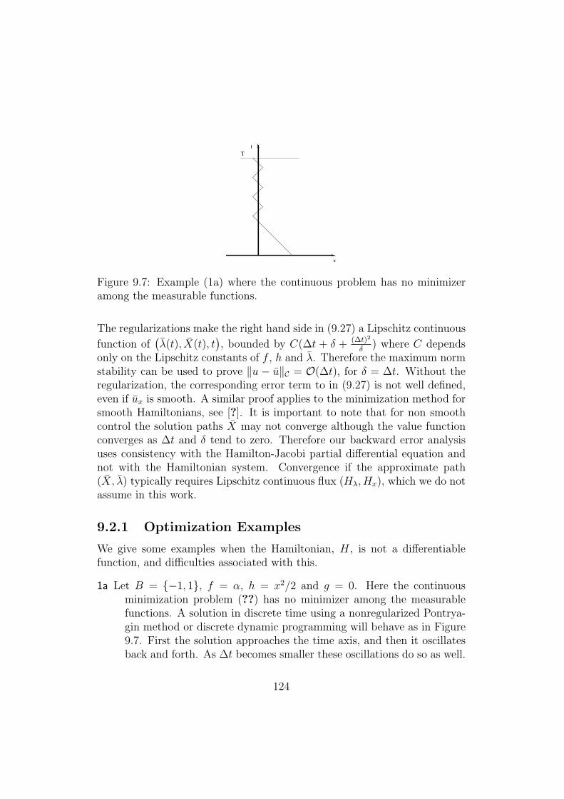
Figure 9.7: Example (1a) where the continuous problem has no minimizeramong the measurable functions.

The regularizations make the right hand side in (9.27) a Lipschitz continuous

function of%#(t), X(t), t

&, bounded by C(#t + ( + (!t)2

% ) where C dependsonly on the Lipschitz constants of f , h and #. Therefore the maximum normstability can be used to prove +u $ u+C = O(#t), for ( = #t. Without theregularization, the corresponding error term to in (9.27) is not well defined,even if ux is smooth. A similar proof applies to the minimization method forsmooth Hamiltonians, see [?]. It is important to note that for non smoothcontrol the solution paths X may not converge although the value functionconverges as #t and ( tend to zero. Therefore our backward error analysisuses consistency with the Hamilton-Jacobi partial di!erential equation andnot with the Hamiltonian system. Convergence if the approximate path(X, #) typically requires Lipschitz continuous flux (H#, Hx), which we do notassume in this work.

9.2.1 Optimization Examples

We give some examples when the Hamiltonian, H, is not a di!erentiablefunction, and di"culties associated with this.

1a Let B = {$1, 1}, f = !, h = x2/2 and g = 0. Here the continuousminimization problem (??) has no minimizer among the measurablefunctions. A solution in discrete time using a nonregularized Pontrya-gin method or discrete dynamic programming will behave as in Figure9.7. First the solution approaches the time axis, and then it oscillatesback and forth. As #t becomes smaller these oscillations do so as well.

124

t

T=1

x

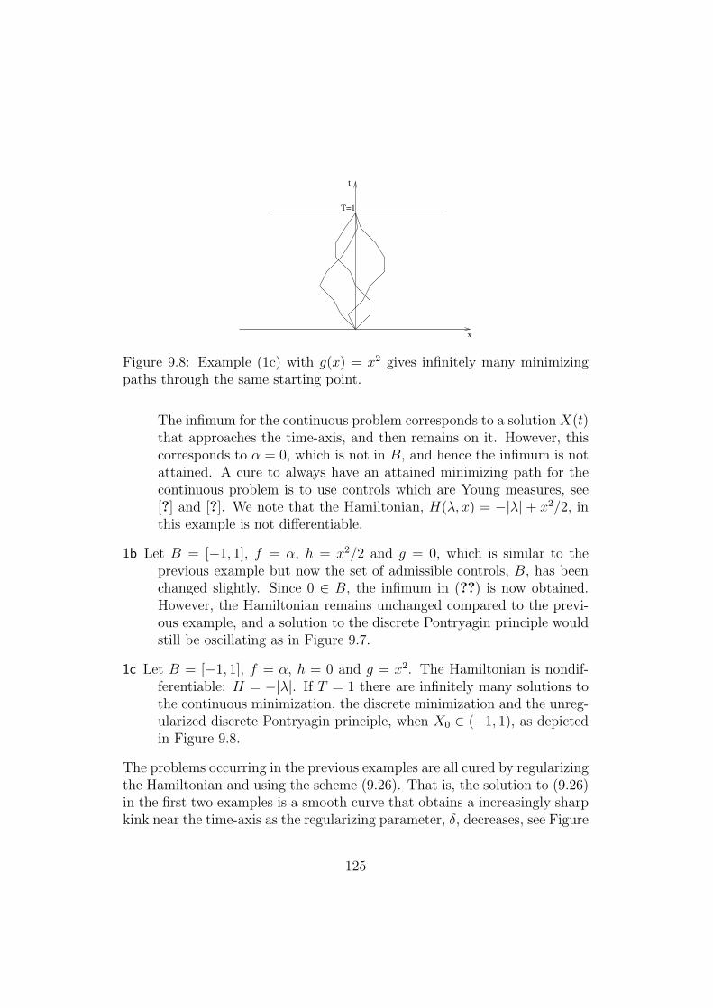
Figure 9.8: Example (1c) with g(x) = x2 gives infinitely many minimizingpaths through the same starting point.

The infimum for the continuous problem corresponds to a solution X(t)that approaches the time-axis, and then remains on it. However, thiscorresponds to ! = 0, which is not in B, and hence the infimum is notattained. A cure to always have an attained minimizing path for thecontinuous problem is to use controls which are Young measures, see[?] and [?]. We note that the Hamiltonian, H(#, x) = $|#| + x2/2, inthis example is not di!erentiable.

1b Let B = [$1, 1], f = !, h = x2/2 and g = 0, which is similar to theprevious example but now the set of admissible controls, B, has beenchanged slightly. Since 0 # B, the infimum in (??) is now obtained.However, the Hamiltonian remains unchanged compared to the previ-ous example, and a solution to the discrete Pontryagin principle wouldstill be oscillating as in Figure 9.7.

1c Let B = [$1, 1], f = !, h = 0 and g = x2. The Hamiltonian is nondif-ferentiable: H = $|#|. If T = 1 there are infinitely many solutions tothe continuous minimization, the discrete minimization and the unreg-ularized discrete Pontryagin principle, when X0 # ($1, 1), as depictedin Figure 9.8.

The problems occurring in the previous examples are all cured by regularizingthe Hamiltonian and using the scheme (9.26). That is, the solution to (9.26)in the first two examples is a smooth curve that obtains a increasingly sharpkink near the time-axis as the regularizing parameter, (, decreases, see Figure

125

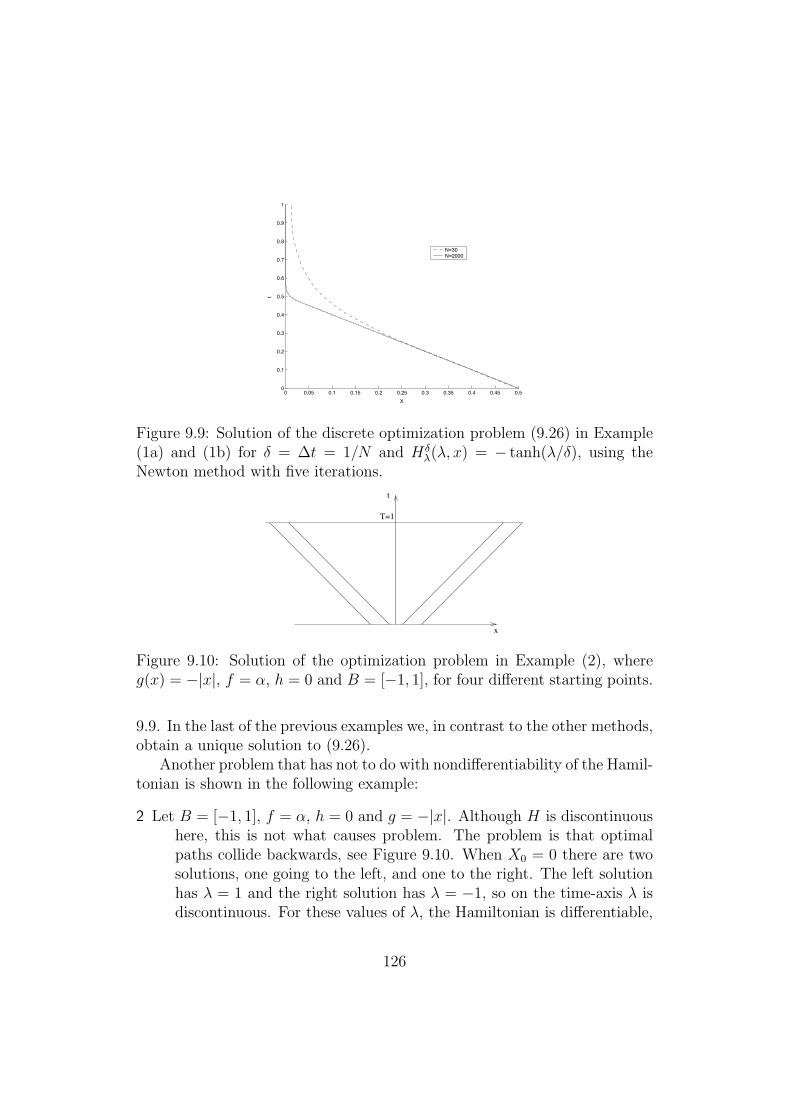
0 0.05 0.1 0.15 0.2 0.25 0.3 0.35 0.4 0.45 0.50

0.1

0.2

0.3

0.4

0.5

0.6

0.7

0.8

0.9

1

X

t

N=30

N=2000

Figure 9.9: Solution of the discrete optimization problem (9.26) in Example(1a) and (1b) for ( = #t = 1/N and H%

#(#, x) = $ tanh(#/(), using theNewton method with five iterations.

t

T=1

x

Figure 9.10: Solution of the optimization problem in Example (2), whereg(x) = $|x|, f = !, h = 0 and B = [$1, 1], for four di!erent starting points.

9.9. In the last of the previous examples we, in contrast to the other methods,obtain a unique solution to (9.26).

Another problem that has not to do with nondi!erentiability of the Hamil-tonian is shown in the following example:

2 Let B = [$1, 1], f = !, h = 0 and g = $|x|. Although H is discontinuoushere, this is not what causes problem. The problem is that optimalpaths collide backwards, see Figure 9.10. When X0 = 0 there are twosolutions, one going to the left, and one to the right. The left solutionhas # = 1 and the right solution has # = $1, so on the time-axis # isdiscontinuous. For these values of #, the Hamiltonian is di!erentiable,

126

therefore the nonsmoothness of the Hamiltonian is not the issue here.It is rather the global properties of the problem that play a role. Thisproblem is di"cult to regularize, and it will not be done here. However,we still can show convergence of the scheme (9.26). This is done inSection ??.

When using (9.26) to solve the minimization problem (??) it is assumedthat the Hamiltonian is exactly known. Is this an unrealistic assumption inpractice? In the following two examples we indicate that there exist inter-esting examples where we know the Hamiltonian. The first has to do withvolatility estimation in finance, and the latter with optimization of an electriccontact.

Implied Volatility

Black-Scholes equation for pricing general options uses the volatility of theunderlying asset. This parameter, however, is di"cult to estimate. One wayof estimation is to use measured market values of options on the consideredasset for standard European contracts. This way of implicitly determiningthe volatility is called implied volatility.

We assume that the financial asset obeys the following Ito stochasticdi!erential equation,

dS(t) = µS(t)dt + )%t, S(t)

&S(t)dW (t), (9.29)

where S(t) is the price of the asset at time t, µ is a drift term, ) is thevolatility and W : R+ " R is the Wiener process. If the volatility is asu"ciently regular function of S, t, the strike level K and the maturity dateT , the so called Dupire equation holds for the option price C(T,K) as afunction of T and K, with the present time t = 0 and stock price S(0) = Sfixed,

CT $ )CKK = 0, T # (0,-), K > 0,

C(0, K) = max{S $K, 0} K > 0,(9.30)

where

)(T,K) ( )2(T,K)K2

2.

Here the contract is an european call option with payo! function max{S(T )$K, 0}. We have for simplicity assumed the bank rate to be zero. The deriva-tion of Dupire’s equation (9.30) is given in [?] and [?].

127

The optimization problem now consists of finding )(T,K) such that

" T

0

"

R+

(C $ C)2(T,K)w(T,K)dKdT (9.31)

is minimized, where C are the measured market values on option prices fordi!erent strike prices and strike times and w is a non negative weight function.In practice, C is not known everywhere, but for the sake of simplicity, weassume it is and set w ( 1, that is there exists a future time T such thatC is defined in R+ ! [0, T ]. If the geometric Brownian motion would be aperfect model for the evolution of the price of the asset, the function )(T,K)would be constant, but as this is not the case, the ) that minimizes (9.31)(if a minimizer exists) varies with T and K.

It is possible to use (??) and (9.26) to perform the minimization of (9.31)over the solutions to a finite di!erence discretization of (9.30)

min&

" T

0

#K,

i

(C $ C)2i dT

subject to"Ci(T )

"T= )D2Ci(T ),

Ci(0) = max(S $ i#K, 0),

(9.32)

where we now let Ci(T ) 3 C(T, i#K) denote the discretized prize function,for strike time T and strike price i#K, and D2 is the standard three pointdi!erence approximation of the second order partial derivative in K, that is(D2C)i = (Ci+1 $ 2Ci + Ci#1)/#K2. In order to have a finite dimensionalproblem we restrict to a compact interval (0, M#K) in K with the boundaryconditions

C0 = S, CM = 0.

The Hamiltonian for this problem is

H(#, C) = #K min&

M#1,

i=1

!#i)i(D

2C)i + (C $ C)2i

#

= #KM#1,

i=1

!min

&i

#i)i(D2C)i + (C $ C)2

i

#

where # is the adjoint associated to the constraint (9.32). We have used thatthe components of the flux, f , in this problem is )i(D2C)i, that the running

128

cost, h, is #K+

i(C $ C)2i , and further that each )i minimizes #i)i(D2C)i

separately, so that the minimum can be moved inside the sum. If we makethe simplifying assumption that 0 * )# * ) * )+ < - we may introduce afunction s : R " R as

s(y) ( min&

y ) =

/y)#, y > 0

y)+, y < 0.

Using s, it is possible to write the Hamiltonian as

H(#, C) = #KM#1,

i=1

!s%#i(D

2C)i

&+

%C $ C

&2

i

#.

Since s is nondi!erentiable, so is H. However, s may easily be regularized,and it is possible to obtain the regularization in closed form, e.g. as in Ex-ample 1. Using a regularized version s% of s, the regularized Hamiltonianbecomes

H%(#, C) = #KM#1,

i=1

!s%

%#i(D

2C)i

&+

%C $ C

&2

i

#,

which using Gateaux derivatives gives the Hamiltonian system

"Ci(T )

"T= s"%

%#i(D

2C)i

&D2Ci(T ), C0 = S CM = 0,

$"#i(T )

"T= D2

!s"%

%#i(D

2C)i

&##

+ 2(C $ C)i,

#0 = #M = 0,

(9.33)

with dataCi(0) = max(S $ i#K, 0), #(T ) = 0.

The corresponding Hamilton-Jacobi equation for the value function

u(C, *) =

" T

'

M#1,

i=1

(C $ C)2i #KdT

is

uT + H(uC , C) = 0, T < T ,

u(T , ·) = 0,

129

!

"

#

!!$%

&

!$'

!$'%

&

&$!%

&$&

&$&%

()

!

!

"

#

!!$%

&

!$*%

!$'

!$'%

&

&$!%

&$&

&$&%

&$"

()

+,

&!!&!

&!!%

&!!

&!!%

&!!#

&!!-

&!!"

"

."/01121/23/42567809/:/5;<7+/50=+7109/:

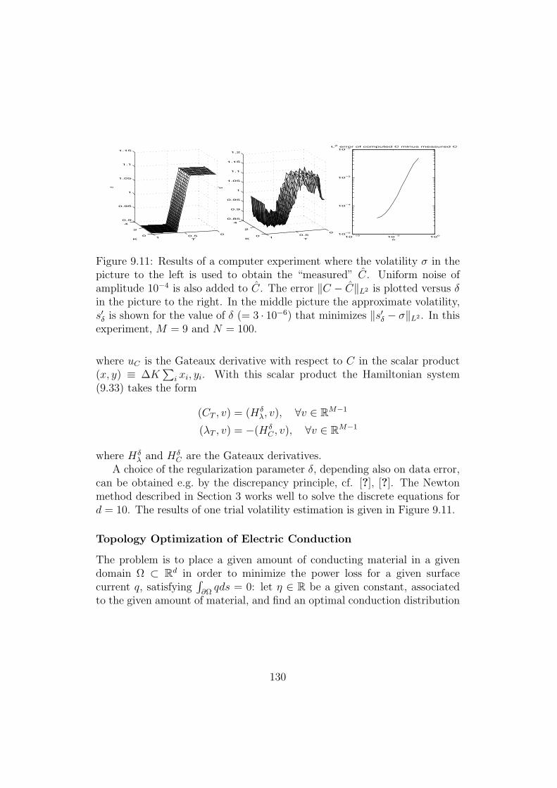
Figure 9.11: Results of a computer experiment where the volatility ) in thepicture to the left is used to obtain the “measured” C. Uniform noise ofamplitude 10#4 is also added to C. The error +C $ C+L2 is plotted versus (in the picture to the right. In the middle picture the approximate volatility,s"% is shown for the value of ( (= 3 · 10#6) that minimizes +s"% $ )+L2 . In thisexperiment, M = 9 and N = 100.

where uC is the Gateaux derivative with respect to C in the scalar product(x, y) ( #K

+i xi, yi. With this scalar product the Hamiltonian system

(9.33) takes the form

(CT , v) = (H%#, v), 4v # RM#1

(#T , v) = $(H%C , v), 4v # RM#1

where H%# and H%

C are the Gateaux derivatives.A choice of the regularization parameter (, depending also on data error,

can be obtained e.g. by the discrepancy principle, cf. [?], [?]. The Newtonmethod described in Section 3 works well to solve the discrete equations ford = 10. The results of one trial volatility estimation is given in Figure 9.11.

Topology Optimization of Electric Conduction

The problem is to place a given amount of conducting material in a givendomain % & Rd in order to minimize the power loss for a given surfacecurrent q, satisfying

$"" qds = 0: let + # R be a given constant, associated

to the given amount of material, and find an optimal conduction distribution

130

) : %" {)#, )+}, where )± > 0, such that

div%)2,(x)

&= 0, x # %, )

",

"n

000""

= q

min&

(

"

""

q, ds + +

"

"

) dx),(9.34)

where "/"n denotes the normal derivative and ds is the surface measure on"%. Note that (9.34) implies that the power loss satisfies

"

""

q, ds = $"

"

div()2,), dx +

"

""

)",

"n, ds

=

"

"

)2, ·2, dx.

The Lagrangian takes the form"

""

q(, + #) ds +

"

"

) (+ $2, ·2#)' () *v

dx

and the Hamiltonian becomes

H(#, ,) = min&

"

"

)v dx +

"

""

q(, + #) ds =

"

"

min&

)v' () *

s(v)

dx +

"

""

q(, + #) ds

with the regularization

H%(#, ,) =

"

"

s%(+ $2, ·2#) dx +

"

""

q(, + #) ds,

depending on the concave regularization s% # C2(R) as in Section 9.2.1. Thevalue function

u(,, *) =

" T

'

(

"

""

q, ds + +

"

"

) dx) dt

for the parabolic variant of (9.34), that is

,t = div%)2,(x)

&,

131

yields the infinite dimensional Hamilton-Jacobi equation

"tu + H("(u, ,) = 0 t < T, u(·, T ) = 0,

using the Gateaux derivative "(u = # of the functional u(,, t) in L2(%).The regularized Hamiltonian generates the following parabolic Hamiltoniansystem for , and #

"

"

%"t,w + s"(+ $2, ·2#)2, ·2w

&dx =

"

""

qw ds"

"

%$ "t#v + s"(+ $2, ·2#)2# ·2v

&dx =

"

""

qv ds

for all test functions v, w # V ( {v # H1(%)00 $

" vdx = 0}. Time indepen-dent solutions satisfy # = , by symmetry. Therefore the electric potentialsatisfies the nonlinear elliptic partial di!erential equation

div%s"%(+ $ |2,|2)2,(x)

&= 0 x # %, s"%

",

"n|"" = q, (9.35)

which can be formulated as the convex minimization problem: , # V is theunique minimizer (up to a constant) of

$! "

"

s%(+ $ |2,(x)|2) dx + 2

"

""

q, ds#. (9.36)

In [?] we study convergence of

limT%&

u(,, t)$ u(,, t)

T,

where u is the value function associated to finite element approximations ofthe minimization (9.36).

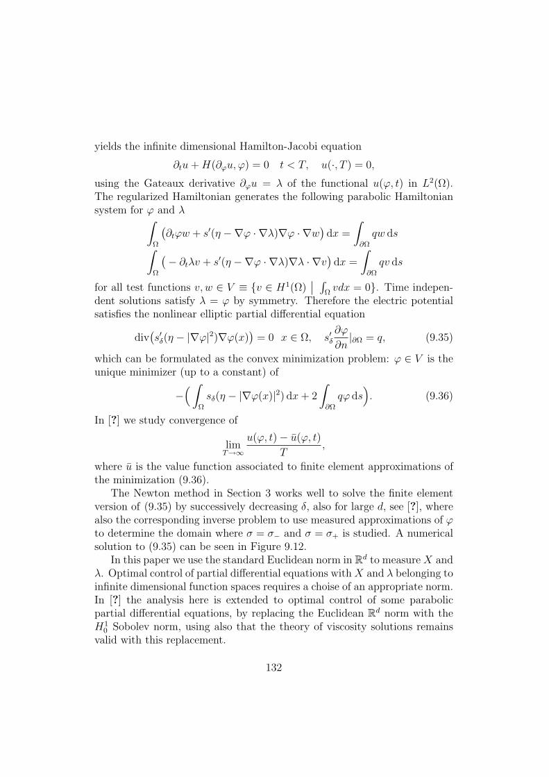
The Newton method in Section 3 works well to solve the finite elementversion of (9.35) by successively decreasing (, also for large d, see [?], wherealso the corresponding inverse problem to use measured approximations of ,to determine the domain where ) = )# and ) = )+ is studied. A numericalsolution to (9.35) can be seen in Figure 9.12.

In this paper we use the standard Euclidean norm in Rd to measure X and#. Optimal control of partial di!erential equations with X and # belonging toinfinite dimensional function spaces requires a choise of an appropriate norm.In [?] the analysis here is extended to optimal control of some parabolicpartial di!erential equations, by replacing the Euclidean Rd norm with theH1

0 Sobolev norm, using also that the theory of viscosity solutions remainsvalid with this replacement.

132

0 0.2 0.4 0.6 0.8 10

0.1

0.2

0.3

0.4

0.5

0.6

0.7

0.8

0.9

1

1 0.001

Figure 9.12: Contour plot of s"% as an approximation of the conductivity ).As seen, % is in this example a square with two circles cut out. Electricalcurrent enters % at two positions on the top of the square and leaves atone position on the bottom. The contours represent the levels 0.2, 0.4, 0.6and 0.8. A piecewise linear FEM was used with 31440 elements, maximumelement diameter 0.01, )# = 0.001, )+ = 1, + = 0.15 and ( = 10#5.

133

9.2.2 Solution of the Discrete Problem

We assume in the theorems that the Pontryagin minimization (9.26) hasbeen solved exactly. In practice (9.26) can only be solved approximatelyby iterations. The simplest iteration method to solve the boundary valueproblem (9.26) is the shooting method: start with an initial guess of #[0] andcompute, for all time steps n, the iterates

Xn+1 = Xn + #tH%#

%#n+1[i], Xn

&, n = 0, . . . , N $ 1, X0 = X0

#n[i + 1] = #n+1[i] + #tH%x

%#n+1[i], Xn

&, n = N $ 1, . . . , 0, #N = gx(XN).

(9.37)

An alternative method, better suited for many boundary value problems,is to use Newton iterations for the nonlinear system F (X, #) = 0 whereF : RNd ! RNd " R2Nd and

F (X, #)2n = Xn+1 $ Xn $#tH%#

%#n+1, Xn

&,

F (X, #)2n+1 = #n $ #n+1 $#tH%x

%#n+1, Xn

&.

(9.38)

An advantage with the Pontryagin based method (9.38) is that the Jacobianof F can be calculated explicitly and it is sparse. The Newton method canbe used to solve the volatility and topology optimization examples in Section2, where the parameter ( is successively decreasing as the nonlinear equation(9.38) is solved more accurately.

Example 9.20 The Newton equations can be solved iterativly, e.g. by ...

Let us use dynamic programming to show that the system (9.26) has asolution in the case that # is a Lipschitz continuous function of (x, t), withLipschitz norm independent of #t, and ( > C#t. One step

x = y + #tH%#

%#(x), y

&(9.39)

for fixed y # Rd has a solution x(y) since the iterations

x[i + 1] = y + #tH%#

%#(x[i]), y

&

yield a contraction for the error e[i] = x[i + m]$ x[i]

e[i + 1] = #t!H%

#

%#(x[i + m]), y

&$H%

#

%#(x[i]), y

&#= #tH%

###xe[i].

134

Conversely, for all x # Rd equation (9.39) has a solution y(x) for each stepsince the iterations

y[i + 1] = x$#tH%#

%#(x), y[i]

&

generate a contraction for the error. The dynamic programming principlethen shows that there are unique paths through all points Xn+1 leading toall Xn for all n.

9.2.3 Convergence of Euler Pontryagin Approximations

Theorem 9.21 Assume that the Hamiltonian H, defined in (??), is Lips-chitz continuous on Rd ! Rd and that (9.26) has a solution (X, #), where#n+1 has uniformly bounded first variation with respect to Xn for all n andall #t, that is there is a constant K such that

|"Xn#n+1| * K. (9.40)

Then the optimal solution, (X, #), of the Pontryagin method (9.26) satisfiesthe error estimate000 inf!!A

!g%X(T )

&+

" T

0

h%X(s), !(s)

&ds

#$

!g(XN) + #t

N#1,

n=0

h%(Xn, #n+1)#000

= O(#t + ( +(#t)2

()

= O(#t), for ( = #t.(9.41)

The bound O(#t) in (9.41) depends on the dimension d through theLipschitz norms of the Hamiltonian H and the constant K in (9.40).

The work [?] presents a convergence result for the case when backwardpaths X(t) collide on a C1 codimension one surface in Rd ! [0, T ]. Thenext subsections give a construction of a regularization H% and the proof ofTheorem 9.21.

Construction of a Regularization

A possible regularization of H is to let H% be a standard convolution molli-fication of H

H%(#, x) =

"

Rd

"

Rd

H(z, y)-%(z $ #)-%(y $ x) dz dy, (9.42)

135

with -% : Rd " R+ a C2 function compactly supported in the ball {y # Rd :|y| * (} and with integral one

$Rd -%(y)dy = 1. This regularization remains

concave in #. Our analysis is not dependent of this specific regularization,but uses that

+H $H%+C + (+H%+C1 + (2+H%+C2 = O((),

and that H% remains a concave function of #.

Convergence without Shocks and Colliding Paths

The proof of the theorem is based on four lemmas. In all of those we supposethat the assumptions of Theorem 9.21 are valid.

Lemma 9.22 The discrete dual function is the gradient of the value func-tion, that is

ux(Xn, tn) = #n. (9.43)

Proof. The relation (9.43) holds for tn = T . Use the induction assumptionthat (9.43) holds true fortN ( T , tN#1, . . . , tn+1. Then the definitions of f % and h% imply

"u

"Xn(Xn, tn) = "Xn

%u(Xn+1, tn+1) + #th%(#n+1, Xn)

&

= "XnXn+1

"u

"Xn+1(Xn+1, tn+1) + #t"Xn

h%(#n+1, Xn)

=%I + #t"Xn

H%#(#n+1, Xn)

&#n+1 + #t"Xn

h%(#n+1, Xn)

= #n+1 + #t"Xn(H%

## + h%)(#n+1, Xn)

$#tH%#(#n+1, Xn)"Xn

#n+1

= #n+1 + #tH%x(#n+1, Xn)

= #n.

Section 9.2.7 shows that (9.43) holds precisely for symplectic methods.We now extend u to be a function defined for all t. First extend the

solution X to all time as a continuous piecewise linear function

X(t) =tn+1 $ t

#tXn +

t$ tn#t

Xn+1, for tn * t < tn+1, (9.44)

136

so that

X "(t) = H%#(#n+1, Xn). (9.45)

The following lemma shows that two di!erent solutions can not collide forsuitable small #t.

Lemma 9.23 There is a positive constant c such that if #t * c( two di!er-ent solutions (X1, #1) and (X2, #2) of (9.26) do not intersect.

Proof. Assume there exist two optimal paths (X1, #1) and (X2, #2) thatintersect at time t, where tn < t * tn+1, then

X1n + (t$ tn)H%

#(#1n+1, X

1n) = X2

n + (t$ tn)H%#(#

2n+1, X

2n)

which can be written

X1n $ X2

n = (t$ tn)%H%

#(#2n+1, X

2n)$H%

#(#1n+1, X

1n)

&. (9.46)

To obtain an estimate of the size of the right hand side in (9.46) integratealong the line

X(s) = X1n + s(X2

n $ X1n),

with #in+1 a function of X i

n. The di!erence in the right hand side of (9.46) is

H%#(#

2n+1, X

2n)$H%

#(#1n+1, X

1n) =

" 1

0

dH%#

dsds

=

" 1

0

%H%

#x + H%##"Xn

#n+1

&ds(X2

n $ X1n).

By assumption it holds that +H%#x + H%

##"Xn#n+1+C = O

%C#(1 + K)/(

&.

Hence the norm of the right hand side in (9.46) is O((#1#t)O11X1

n $ X2n

11.Therefore there is a positive constant c such that if #t < c(, the equation(9.46) has only the solution X1

n = X2n.

Since the optimal paths X do not collide, for suitable small #t, the valuefunction u is uniquely defined along the optimal paths, by (9.28) and

u%X(t), t

&= u(Xn+1, tn+1) + (tn+1 $ t)h%(Xn, #n+1), tn < t < tn+1 (9.47)

and we are ready for the main lemma

137

Lemma 9.24 The value function for the Pontryagin method satisfies a Hamilton-Jacobi equation close to (9.67), more precisely there holds

ut + H(ux, ·) = O(( + #t +(#t)2

() in Rd ! (0, T ),

u = g on Rd.(9.48)

The error term O((+#t+ (!t)2

% ) in (9.48) is a Lipschitz continuous functionof ux(x, t), x and t satisfying

|O(( + #t +(#t)2

()| * CC#

!( + Cx#t + CxC#(1 + K)

(#t)2

(

#,

where Cx and C# are the Lipschitz constants of H in the x and # variable,respectively, and C 5 1 does not depend on the data.

Proof. The proof starts with the observation

0 =d

dtu(X(t), t) + h%(#n+1, Xn)

= ut(X(t), t) + ux(X(t), t) · f %(#n+1, Xn) + h%(#n+1, Xn).(9.49)

The idea is now to use that the dual function # is the gradient of u at the timelevels tn, by Lemma 9.22, (and a good approximation at times in between)and that the modified discrete Pontryagin method shows that the right handside in (9.49) is consistent with the correct Hamiltonian H.

We will first derive an estimate of |ux(X(t), t)$ #n+1| for tn < t < tn+1.We have that

u(X(t), t) = u(Xn+1, tn+1) + (tn+1 $ t)h%(#n+1, Xn)

Therefore ux(X(t), t) can be written as

ux(X(t), t) ="Xn

"Xt

!"Xn+1

"Xnux(Xn+1, tn+1) + (tn+1 $ t)"Xn

h%(#n+1, Xn)#

="Xn

"Xt

!"Xn+1

"Xn#n+1 + (tn+1 $ t)"Xn

h%(#n+1, Xn)#.

Introduce the notation

A ( "XnH%

#(#n+1, Xn) = H%#x(#n+1, Xn) + H%

##(#n+1, Xn)"Xn#n+1

= O%C#(1 + K)/(

&.

(9.50)

138

We have

"Xn+1

"Xn= I + #tA = I + (t$ tn)A + (tn+1 $ t)A

"Xn

"Xt=

%I + (t$ tn)A

&#1

therefore as in Lemma 9.22

ux(X(t), t)

= #n+1 + (tn+1 $ t)%I + (t$ tn)A

&#1%A#n+1 + "Xn

h%(#n+1, Xn)&

= #n+1 + (tn+1 $ t)%I + (t$ tn)A

&#1H%

x(#n+1, Xn)

= #n+1 + O%Cx#t + CxC#(K + 1)(#t)2/(

&.

(9.51)

Introduce the notation # ( ux(X(t), t) and split the Hamiltonian term in(9.49) into three error parts:

r(#, X(t), t) ( #f %(#n+1, Xn) + h%(#n+1, Xn)$H%#, X(t)

&

= #f %(#n+1, Xn) + h%(#n+1, Xn)$H%(#, Xn)

+ H%(#, Xn)$H%%#, X(t)

&

+ H%%#, X(t)

&$H

%#, X(t)

&

( I + II + III.

(9.52)

Taylor expansion of H% to second order and (9.51) show

|I| = |H%(#n+1, Xn) + (#$ #n+1)H%#(#n+1, Xn)$H%(#, Xn)|

* min%2C#|#$ #n+1|, |(#$ #n+1)H

%##(., Xn)(#$ #n+1)|/2

&

* CC#

%Cx#t + CxC#(K + 1)(#t)2/(

&;

the Lipschitz continuity of H% implies

|II| * |H%x||X(t)$ Xn| * |H%

x||H%#|#t;

and the approximation H% satisfies

|III| * CC#(.

The combination of these three estimates proves (9.48).

139

To finish the proof of the lemma we show that the error function r can beextended to a Lipschitz function in Rd!Rd! [0, T ]. We note that by (9.40),(9.44) and (9.51) # is a Lipschitz function of Xt and t, and r(#(Xt, t), Xt, t)is Lipschitz in Xt and t. By

r(#, X, t) ( r(#(X, t), X, t)

we obtain a Lipschitz function r in Rd ! Rd ! [0, T ].The results in these lemmas finishes the proof of Theorem 9.21: the com-

bination of the residual estimates in Lemma 9.24 and the C-stability estimateof viscosity solutions in Lemma 9.25 proves the theorem.

The approximation result can be extended to the case when the set ofbackward optimal paths {(X(t), t) : t < T}, solving (9.26) and (9.44) , maycollide into a codimension one surface $ in space-time Rd ! [0, T ], see [?].

Maximum Norm Stability for Hamilton-Jacobi Equations

The seminal construction of viscosity solutions by Crandall and Lions [?]also includes C stability results formulated in a general setting. We restatea variant adapted to the convergence results in this paper.

Lemma 9.25 Suppose H : Rd!Rd " R is a Lipschitz continuous Hamilto-nian satisfying for a constant C and for all x, x, #, # # Rd

|H(#, x)$H(#, x)| * Cx|x$ x|(1 + |#|),|H(#, x)$H(#, x)| * C#|#$ #|.

Suppose also that e : Rd ! [0, T ] " R and g : Rd " R are Lipschitz continu-ous. Then, the bounded uniformly continuous viscosity solutions u and u ofthe Hamilton-Jacobi equations

ut + H(ux, ·) = 0 in Rd ! (0, T ), u|Rd){T} = g, (9.53)

ut + H(ux, ·) = e in Rd ! (0, T ), u|Rd){T} = g, (9.54)

satisfy the C-stability estimate

O +u$ u+C(Rd)[0,T ]) * TO +e+C(Rd)[0,T ]) . (9.55)

This follows from the maximum norm stability (9.19), but other proofsbased on the maximum principle or the comparison principle are also possible,see [?].

140

9.2.4 How to obtain the Controls

The optimal control for the exact problem (9.67) is determined by the valuefunction through the Pontryagin principle

!(x, t) # argmina!B

%ux(x, t) · f(x, a) + h(x, a)

&.

Assume we have solved a discrete approximating optimal control problem andobtained the approximations X, # and u. Can they be used to determine anapproximation of the control !? Even in the case that the optimal controlS(#, x) ( argmina

%# · f(x, a) + h(x, a)

&is a function, it is in general not

continuous as function of x and # but only piecewise Lipschitz continuous.Therefore the approximate control S(#(t), x) cannot be accurate in maximumnorm. However, weaker measures of the control can converge; for instancethe value function is accurately approximated in Theorems 9.21 and ??.At the points where S is Lipschitz continuous the error in the control isproportional to the error |#(x, t) $ ux(x, t)|, for fixed x. If we assume thatthe error u(·, t) $ u(·, t) is bounded by $ in a

,$-neighborhood of x and

that uxx and uxx also are bounded there, we obtain, for di!erence quotients#u/#x and |#x| =

,$, the error estimate

#$ ux = #$ #u

#x+

#u

#x$ #u

#x+

#u

#x$ ux = O(#x + $/#x) = O(

,$).

Convergence of the approximate path (X, #) typically requires Lipschitz con-tinuous flux (H#, Hx), which we do not assume in this work.

9.2.5 Inverse Problems and Tikhonov Regularization

One way to introduce regularization of ill-posed inverse problems is to studya simple example such as u" = f : the forward problem to determine u fromf in this case becomes a well-posed integral u(x) = u(0) +

$ x

0 f(s)ds andthe inverse problem is then to determine f from u by the derivative f = u".Note that a small error in the data can be amplified when di!erentiated;for instance a small perturbation maximum-norm $ sin(-x) in u leads to thef -perturbation $- cos(-x) which is large (in maximum-norm) if -$% 1 evenif $ 6 1, while a small maximum-norm perturbation of f leads to a smallperturbation of u (in maximum norm). This is the reason that, to determineu from f is well posed (in maximum norm), while the inverse problem todetermine f from u is ill posed.

141

The simplest method to regularize the problem f = u" is to replace thederivative with a di!erence quotient with suitable step size h. If we assumethat our measured values u$ of u # C2 are polluted with an error + of size $in maximum norm so that u$ = u + +, we have

f = (u$ $ +)".

To avoid di!erentiating + we use the di!erence quotient

f(x) = u"(x)

=u(x + h)$ u(x)

h+ O(h)

=u$(x + h)$ u$(x)

h+ O($h#1 + h).

The error term is minimal if we choose h2 7 $, that is the optimal step size,h 7

,$, yields the error O($1/2) to compute f by the di!erence quotient.

This di!erence quotient converges to u" as $ tends to zero. If we take toosmall step size (e.g. h = $), the estimation error does not tend to zero as themeasurement error tends to zero.

We can write the inverse problem u" = f as the optimal control problem

X t = !t,

min!:(0,1)%[#M,M ]

2#1

" 1

0

|X t $X t$|2 dt,

where we changed notation to t := x, X = u, X$ = u$, ! := f and put theconstraint to seek ! in the bounded set [$M, M ] for some positive M . TheHamiltonian becomes

H(#, x, t) = min!![#M,M ]

%# · ! + 2#1|x$X t

$|2&

= $M |#| + 2#1|x$X t$|2

which is not di!erentiable and leads to the system

X t = $Msgn(#)

#t = $(X t $X t$).

A regularization of this is to replace sgn# by tanh #/( in the flux, whichyields the regularized Hamiltonian

H%(#, x, t) = $M( log(cosh#

() + 2#1|x$X t

$|2. (9.56)

142

A standard alternative and related regularization is to add a penaltyfunction depending on the control to the Lagrangian

L%(#, x,!) :=

" 1

0

#t(!t $ X t) + 2#1|X t $X t$|2 + (!2 dt

for some ( > 0, which generates the Hamiltonian system

X t = $Msgn%(#)

#t = $(X t $X t$),

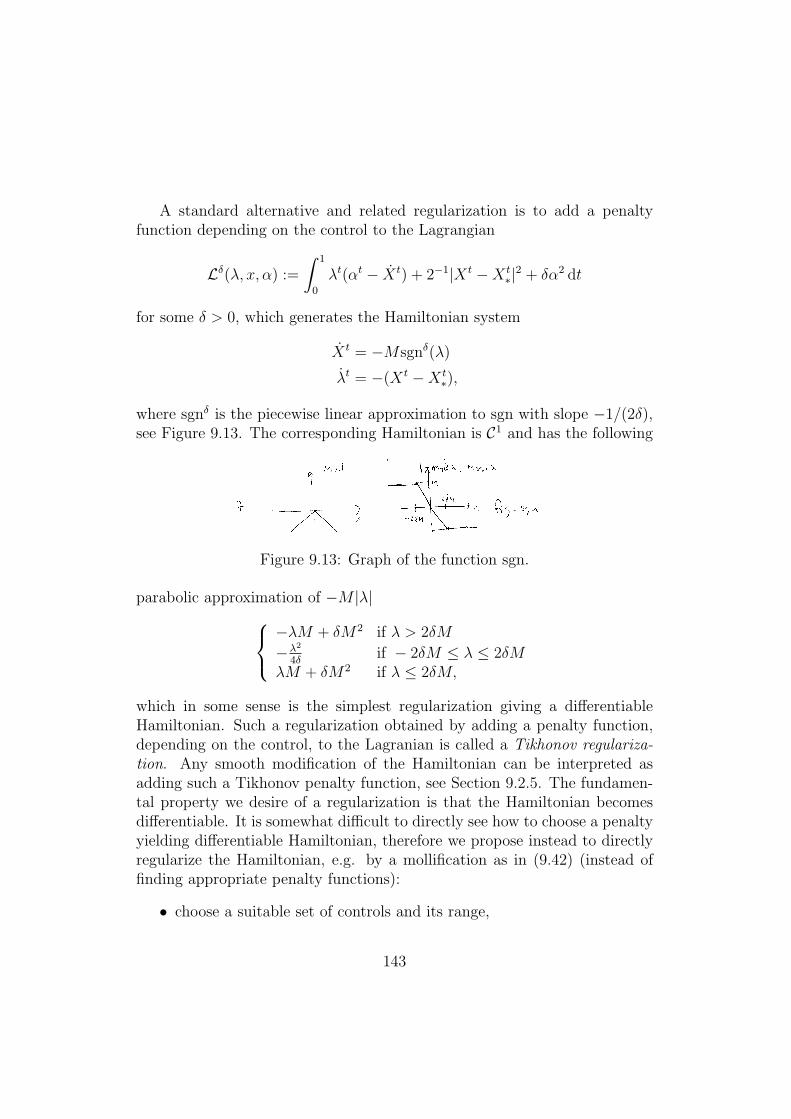
where sgn% is the piecewise linear approximation to sgn with slope $1/(2(),see Figure 9.13. The corresponding Hamiltonian is C1 and has the following

r\-I-i dty i"'

I - |

\ /

/L--

i t' t

,b i15 _

+

K-. rof4l , r i

i

ks**&

t * v,.t:Ay

f . ^i;r - fi'Uvu vrt4

J 'J

k^

eq*1

"- l"ti r.1

1

^ v/ , '

_-d

#;:I

i

f,, )

'tiu+-

1#

I

l i

r,

r4'.

- --t---),"1

'', /

/ \

1n'J' t

Y,

ril t

z {n1

Oy b u,,4 puirrt

Figure 9.13: Graph of the function sgn.

parabolic approximation of $M |#|23

4

$#M + (M2 if # > 2(M$#2

4% if $ 2(M * # * 2(M#M + (M2 if # * 2(M,

which in some sense is the simplest regularization giving a di!erentiableHamiltonian. Such a regularization obtained by adding a penalty function,depending on the control, to the Lagranian is called a Tikhonov regulariza-tion. Any smooth modification of the Hamiltonian can be interpreted asadding such a Tikhonov penalty function, see Section 9.2.5. The fundamen-tal property we desire of a regularization is that the Hamiltonian becomesdi!erentiable. It is somewhat di"cult to directly see how to choose a penaltyyielding di!erentiable Hamiltonian, therefore we propose instead to directlyregularize the Hamiltonian, e.g. by a mollification as in (9.42) (instead offinding appropriate penalty functions):

• choose a suitable set of controls and its range,

143

• determine the Hamiltonian,

• mollify the Hamiltonian with a parameter ( > 0 as in (9.42).

Another example of a forward problem is to determine the solution u,representing e.g. temperature, in the boundary value problem

%a(x)u"(x)

&"= f(x) 0 < x < 1

u(0) = u"(1) = 0

for a given source function f : (0, 1) " (c,-) and a given conductivitya : (0, 1) " (c,-) with c > 0. This is a well posed problem with thesolution

u(x) =

" x

0

F (s)$ F (1)

a(s)ds,

where F (s) =$ s

0 f(t) dt is a primitive function of f . The inverse problem tofind the conductivity a from given temperature u and source f leads to

a(x) =F (x)$ F (1)

u"(x),

which depends on the derivative u", as in the previous example, so that it isill posed (in maximum norm) by the same reason.

Example 9.26 [ ] Condition number, matrices, tomography

9.2.6 Smoothed Hamiltonian as a Tikhonov Regular-ization

The C2 regularization of the Hamiltonian can also be viewed as a specialTikhonov regularization, using the Legendre transformation: a preliminaryidea is to find the Tikhonov penalty function T (x, !) : Rd!A" R such that

min!!A

%# · f(x, !) + T (x, !)

&= H%(#, x).

In general this can only hold if the set A is dense enough, e.g. if A wouldconsist of only two elements the function H% would not be smooth. Thereforewe replace A seeking the minimum in the convex closure

5f(x, A) := {sf1 + (1$ s)f2 | s # [0, 1], and f1, f2 # f(x, A)}

144

and we instead want to find Tx(f) : Rd ! 5f(x, A)" R such that

min)! bf(x,A)

%# · / + Tx(/)

&= H%(#, x) for all # # Rd. (9.57)

To find the Tikhonov penalty, the first step is to observe that by Theorem ??there is for each #, where "#H(·, x) is defined, an ! such that "#H(#, x) =f(x, !); therefore the regularization H%(#, x) =

$Rd H(# $ y)+(y)dy, as in

(??), satisfies "#H%(Rd, x) & 5f(x, A), since H is Lipschitz continuous andhence di!erentiable almost everywhere. Define the Legendre transformation

Tx(/) := sup#!Rd

!$ # · / + H%(#, x)

#for all / # Rd. (9.58)

Figure 9.14 illustrates the value of the Legendre transform

T (/) = sup#!R

!$ # · / + H(#)

#

of a concave di!erentiable function H : R " R: find the tangent to the curve{%#, H(#)

&| # # R} with the slope /, then its intersection with the y-axis

is T (/); in multi dimension, d ) 1, find the tangent plane of the graph of Hwith normal (/,$1), then the point (0, T (/)) is in the plane. If the range of"#H(·, x) is only a subset S of Rd, we see that T (/) = +- for / # Rd $ S.

Figure 9.14: Illustratation of the Legendre transfrom.

Theorem 9.27 By defining Tx(/) := Tx(/), the relation (9.57) holds.

Proof. Fix a point x # Rd. The definition (9.58) of the Legendre transformimplies that for any / and all # # Rd we have

# · / + Tx(/) ) H%(#, x). (9.59)

It remains to show that for any # we can have equality here by choosing /precisely.

Since the Hamiltonian H%(·, x) is concave and di!erentiable, with "#H%(·, x) #5f(x, A), the maximum in the Legendre transform is, for / in the interior of5f(x, A), attained at a point #$ (depending on /) satisfying

Tx(/) = sup#!Rd

%$ # · / + H%(#, x)

&= $#$ · / + H%(#$, x)

145

and / = "#H%(#$, x), so that the choise / = "#H%(#, x) gives equality in(9.59). The fact that Tx is lower semicontinuous shows that

inf)! interior bf(x,A)

%# · / + Tx(/)

&= min

)! bf(x,A)

%# · / + Tx(/)

&.

!

Exercise 9.28 [ ] Show that Tikhonov penalty for the regularized Hamilto-nian (9.56) in the u" = f problem is

(M2

2

!(1 +

!

M) log((1 +

!

M) + (1$ !

M) log(1$ !

M)#

+1

2|x$X t

$|2.

9.2.7 General Approximations

The essential property of the symplectic Euler method we have used is thatux(Xn, tn) = #n. This relation holds precisely for symplectic approximations(cf. Remark 9.30):

Theorem 9.29 Consider a general one step method

Xn+1 = A(#n+1, Xn)

#n = C(#n+1, Xn)(9.60)

with

u(Xn, tn) = g(XN) +N#1,

m=n

B(#n+1, Xn)#t.

Then ux(Xn, tn) = #n, for all n, implies that the mapping / : (Xn, #n) 8"(Xn+1, #n+1) is symplectic. If / is symplectic it is possible to choose thefunction B so that ux(Xn, tn) = #n, for all n.

Proof. As in Lemma 9.22 we have

ux(Xn, tn) =dA

%Xn, #n+1(Xn)

&

dXnux(Xn+1, tn+1) +

dB%Xn, #n+1(Xn)

&

dXn.

Therefore the relationux(Xn, tn) = #n

146

holds if and only if #A# +B# = 0 and #Ax +Bx = C. Let S ( #A+B. Then#A# + B# = 0 is equivalent to S# = A, but S# = A implies B = S $ #S#

so that #Ax + Bx = Sx. Therefore #A# + B# = 0 and #Ax + Bx = C isequivalent to A = S# and C = Sx.

Let S ( #n+1 · Xn + #tH(#n+1, Xn). Then (9.60), with A = S# andC = Sx, becomes

Xn+1 = Xn + #tH#(Xn, #n+1)

#n = #n+1 + #tHx(Xn, #n+1),(9.61)

which by Remark 9.30 is equivalent to symplecticity of the mapping (Xn, #n) 8"(Xn+1, #n+1).

Remark 9.30 A one step method (9.60), interpreted as

(Xn, #n) 8" (Xn+1, #n+1),

is called symplectic if there exists a function H(#n+1, Xn) such that (9.61)holds, see Theorem 5.1, Lemma 5.2 and (5.5) in Chapter VI of [?], where athorough study on symplectic methods can be found.

To generalize the error estimate of Theorems 9.21 and ?? to general sym-plectic one step approximations (9.61), e.g. the second order symplecticRunge-Kutta method

H =1

2

!H(#n+1, Xn) + H

%#n+1 + #tHx(#n+1, Xn), Xn + #tH#(#n+1, Xn)

&#

requires first an extension of Xn and u to all time, by approximations (f , h)of (f %, h%) with

dX

dt= f and

du

dt= $h,

and then an estimate of the residual error r as in (9.52). In practice weneed more regularity of H% to take advantage of higher order methods. Sincewe only have Lipschitz bounds of H the estimate of r is not smaller thanthe error h% $ h, which is O(+H%+Cp)(#t)p = O((#t)p/(p#1) for a pth orderaccurate method. Consequently the residual error is not smaller than O(( +(#t)p/(p#1) = O(#t) for ( 7 #t, so that our error estimate does not improvefor higher order schemes, without additional assumptions. On the other hand

147

by extending X as a piecewise linear function, as before, the only change ofthe analysis in Sections 9.2.3 and ?? to other symplectic methods (9.61) isto replace H%(#n+1, Xn) by H(#n+1, Xn) and since

+H% $ H+C + (+H% $ H+C1 + (2+H% $ H+C2 = O(#t)

the estimate (9.48) holds for all symplectic methods which are at least firstorder accurate.

Similarly, by considering (Xn+1, #n), instead of (Xn, #n+1), as independentvariables the scheme

Xn = A(Xn+1, #n)

#n+1 = C(Xn+1, #n),

is symplectic if and only if

Xn = Xn+1 $#tH#(Xn+1, #n)

#n+1 = #n $#tHx(Xn+1, #n),(9.62)

and the error analysis of the methods (9.61) applies with

H(Xn, #n+1) = (Xn+1 $ Xn) · (#n+1 $ #n) + H(Xn+1, #n).

An example of a method (9.62) is the Euler method H = H, which is back-ward Euler for X forwards in time and backward Euler for # backwards intime, in contrast to (9.26) which is forward Euler for X forwards in time andforward Euler for # backwards in time.

9.3 Optimal Control of Stochastic Di!eren-tial Equations

In this section we study optimal control of the solution X(t) to the stochasticdi!erential equation6

dXi = ai(X(s), !(s, X(s)))dt + bij(X(s), !(s, X(s)))dWj, t < s < TX(t) = x

(9.63)

where T is a fixed terminal time and x # Rn is a given initial point. Assumethat ai, bij : Rn ! A" R are smooth bounded functions, where A is a given

148

compact subset of Rm. The function ! : [0, T ] ! Rn " A is a control andlet A be the set of admissible Markov control functions t" !(t, X(t)). TheMarkov control functions use the current value X(s) to a!ect the dynamicsof X by adjusting the drift and the di!usion coe"cients. Let us for theseadmissible controls ! # A define the cost

Ct,x(!) = E[

" T

t

h(X(s), !(s))ds + g(X(T ))]

where X solves the stochastic di!erential equation (9.63) with control ! and

h : Rn ! A" R, g : Rn " R

are given smooth bounded functions. We call h the running cost and g theterminal cost. Our goal is to find an optimal control !$ which minimizes theexpected cost, Ct,x(!).

Let us define the value function

u(t, x) ( inf!!A

Ct,x(!). (9.64)

The plan is to show that u solves a certain Hamilton-Jacobi equation andthat the optimal control can be reconstructed from u. We first assume forsimplicity that the optimal control is attained, i.e

u(t, x) = min!!A

Ct,x(!) = Ct,x(!$).

The generalization of the proofs without this assumption is discussed in Ex-ercise 9.37.

9.3.1 An Optimal Portfolio

Example 9.31 Assume that the value of a portfolio, X(t), consists of riskystocks, S(t) = !(t)X(t), and risk less bonds, B(t) = (1 $ !(t))X(t), where!(t) # [0, 1] and

dS = aSdt + cSdW, (9.65)

dB = bBdt, (9.66)

149

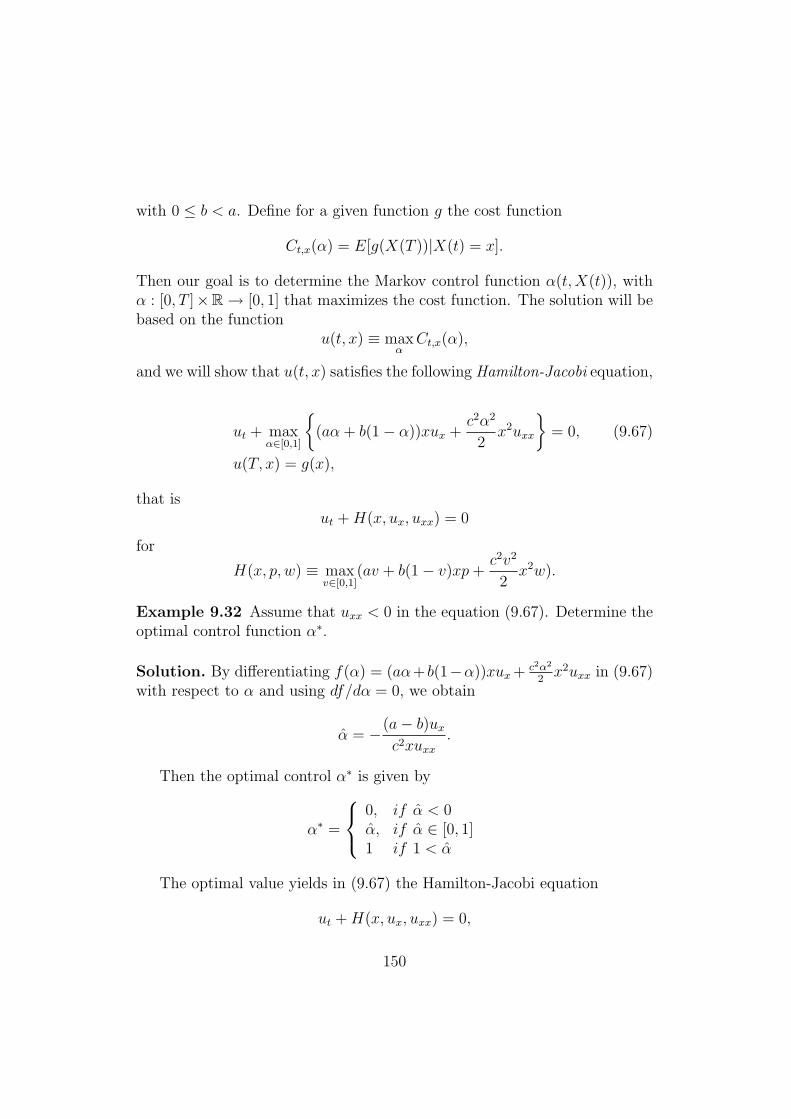
with 0 * b < a. Define for a given function g the cost function

Ct,x(!) = E[g(X(T ))|X(t) = x].

Then our goal is to determine the Markov control function !(t, X(t)), with! : [0, T ]!R " [0, 1] that maximizes the cost function. The solution will bebased on the function

u(t, x) ( max!

Ct,x(!),

and we will show that u(t, x) satisfies the following Hamilton-Jacobi equation,

ut + max!![0,1]

6(a! + b(1$ !))xux +

c2!2

2x2uxx

7= 0, (9.67)

u(T, x) = g(x),

that isut + H(x, ux, uxx) = 0

for

H(x, p, w) ( maxv![0,1]

(av + b(1$ v)xp +c2v2

2x2w).

Example 9.32 Assume that uxx < 0 in the equation (9.67). Determine theoptimal control function !$.

Solution. By di!erentiating f(!) = (a!+ b(1$!))xux + c2!2

2 x2uxx in (9.67)with respect to ! and using df/d! = 0, we obtain

! = $(a$ b)ux

c2xuxx.

Then the optimal control !$ is given by

!$ =

23

4

0, if ! < 0!, if ! # [0, 1]1 if 1 < !

The optimal value yields in (9.67) the Hamilton-Jacobi equation

ut + H(x, ux, uxx) = 0,

150

where

H(x, ux, uxx) =

288883

88884

bxux, if ! < 0

bxux $(a$ b)2u2

x

2c2uxx, if ! # [0, 1]

axux +c2x2uxx

2if 1 < !

(9.68)

!

Example 9.33 What is the optimal control function ! = !$ for g(x) =xr, 0 < r < 1 ?

Solution. We have dX = d(!X + (1 $ !)X) = dS + dB = (aS + bB)dt +cSdW = (a!X + b(1$ !)X)dt + c!XdW , so that the Ito formula yields

dg(X) = dXr = rXr#1dX +r(r $ 1)

2Xr#2(dX)2

= rXr(a! + b(1$ !))dt + rXr!cdW +1

2!2c2r(r $ 1)Xrdt.

Taking the expectation value in the above,

E[Xr(T )] = Xr(0) + E

9" T

0

rXr

:a! + b(1$ !) +

1

2!2c2(r $ 1)

;dt

<.

Finally, perturb the above equation with respect to $ # R+ provided ! =!$+$v for some feasible function v, that is !$+$v # [0, 1] for su"ciently small$. Then the optimal control, !$, should satisfy E[Xr

!"+$v(T )]$E[Xr!"(T )] *

0 4v. If we make the assumption !$ # (0, 1), then we obtain

E[

" T

0

rXrv(a$ b + !$c2(r $ 1))dt] = 0, 4v

which implies

!$ =a$ b

c2(1$ r).

!

Exercise 9.34 What is the optimal control in (9.67) for g(x) = log x ?

151

9.3.2 Dynamic Programming and Hamilton-Jacobi Equa-tions

Lemma 9.35 Assume that the assumptions in section 9.3.1 hold. Then, thefunction u satisfies, for all ( > 0, the dynamic programming relation

u(t, x) = min!:[t,t+%]%A

E[

" t+%

t

h(X(s), !(s, X(s)))ds + u(t + (, X(t + ())].(9.69)

Proof. The proof has two steps: to use the optimal control to verify

u(t, x) ) min!!A

E[

" t+%

t

h(X(s), !(s))ds + u(t + (, X(t + ())],

and then to show that an arbitrary control yields

u(t, x) * min!!A

E[

" t+%

t

h(X(s), !(s))ds + u(t + (, X(t + ())],

which together imply Lemma 9.35.Step 1: Choose the optimal control !$, from t to T , to obtain

u(t, x) = min!!A

E

9" T

t

h(X(s), !(s, X(s)))ds + g(X(T ))

<

= E[

" t+%

t

h(X(s), !$(s))ds] + E[

" T

t+%

h(X(s), !$(s))ds + g(X(T ))]

= E[

" t+%

t

h(X(s), !$(s))ds]

+E

9E[

" T

t+%

h(X(s), !$(s))ds + g(X(T ))| X(t + ()]

<

) E[

" t+%

t

h(X(s), !$(s))ds] + E[u(X(t + (), t + ()]

) min!!A

E

9" t+%

t

h(X(s), !(s, X(s))ds + u(X(t + (), t + ()

<.

Step 2: Choose the control !+ to be arbitrary from t to t + ( and then,given the value X(t + (), choose the optimal !$ from t + ( to T . Denote this

152

control by !" = (!+, !$). Definition (9.64) shows

u(t, x) * Ct,x(!")

= E[

" T

t

h(X(s), !"(s))ds + g(X(T ))]

= E[

" t+%

t

h(X(s), !+(s))ds] + E[

" T

t+%

h(X(s), !$(s))ds + g(X(T ))]

= E[

" t+%

t

h(X(s), !+(s))ds]

+E

9E[

" T

t+%

h(X(s), !$(s))ds + g(X(T ))| X(t + ()]

<

= E[

" t+%

t

h(X(s), !+(s))ds] + E[u(X(t + (), t + ()].

Taking the minimum over all controls !+ yields

u(t, x) * min!+!A

E

9" t+%

t

h(X(s), !+(s))ds + u(X(t + (), t + ()

<.

!

Theorem 9.36 Assume that X solves (9.63) with a Markov control function! and that the function u defined by (9.64) is bounded and smooth. Then usatisfies the Hamilton-Jacobi equation

ut + H(t, x,Du, D2u) = 0,

u(T, x) = g(x),

with the Hamiltonian function

H(t, x,Du, D2u) ( min!!A

9ai(x, !)"xiu(t, x) +

bik(x, !)bjk(x, !)

2"xixju(t, x) + h(x, !)

<

Proof. The proof has two steps: to show that the optimal control ! = !$

yields

ut + a$i "xiu +b$ikb

$jk

2"xixju + h$ = 0, (9.70)

153

where a$(x) = a(x, !$(t, x)), b$(x) = b(x, !$(t, x)) and h$(t, x) = h(t, x,!$(t, x)),and then that an arbitrary control !+ implies

ut + a+i "xiu +

b+ikb

+jk

2"xixju + h+ ) 0, (9.71)

where a+(x) = a(x, !+(t, x)), b+(x) = b(x, !+(t, x)) and h+(t, x) = h(t, x,!+(t, x)).The two equations (9.70) and (9.71) together imply Theorem 9.36.

Step 1 : Choose ! = !$ to be the optimal control in (9.63). Then bythe dynamic programming principle of Lemma 9.64

u(X(t), t) = E[

" t+%

t

h(X(s), !$(s, X(s)))ds + u(X(t + (), t + ()],

so that Ito ’s formula implies

$h(t, x,!$(t, x))dt = E[du(X(t), t)| X(t) = x] (9.72)

= (ut + a$i "xiu +b$ikb

$jk

2"xixju)(t, x)dt.

Definition (9.64) showsu(T, x) = g(x),

which together with (9.72) prove (9.70).Step 2 : Choose the control function in (9.63) to be arbitrary from time

t to t + ( and denote this choice by ! = !+. The function u then satisfies byLemma 9.64

u(t, x) * E[

" t+%

t

h(X(s), !+(s))ds] + E[u(X(t + (), t + ()].

Hence E[du] ) $h(x, !+)dt. We know that for any given !+, by Ito ’sformula,

E[du(t, X(t))] = E

=ut + a+

i "xiu +b+ikb

+jk

2"xixju

>dt.

Therefore, for any control !+,

ut + a+i "xiu +

b+ikb

+jk

2"xixju + h(x, !+) ) 0,

which proves (9.71) !

154

Exercise 9.37 Use a minimizing sequence !i of controls, satisfying

u(t, x) = limi%&

Ct,x(!i),

to prove Lemma 9.64 and Theorem 9.36 without the assumption that theminimum control is attained.

Exercise 9.38 Let A+ be the set of all adapted controls {! : [0, T ] !C[0, T ] " A} where !(s, X) may depend on {X(*) : * * s}. Show thatthe minimum over all adapted controls in A+ is in fact the same as theminimum over all Markov controls, that is

inf!!A+

Ct,x(!) = inf!!A

Ct,x(!),

e.g. by proving the dynamic programming relation (9.69) for adapted controlsand motivate why this is su"cient.

9.3.3 Relation of Hamilton-Jacobi Equations and Con-servation Laws

In this section we will analyze qualitative behavior of Hamilton-Jacobi equa-tions, in particular we will study the limit corresponding to vanishing noisein control of stochastic di!erential equations. The study uses the relationbetween the Hamilton-Jacobi equation for V : [0, T ]! R " R

Vt + H(Vx) = 0, V (0, x) = V0(x), (H $ J)

and the conservation law for U : [0, T ]! R " R

Ut + H(U)x = 0, U(0, x) = U0(x). (C $ L)

Observe that the substitution V (t, x) =$ x

#& U(t, y)dy, so that U = Vx, andintegration in x from $- to x in (C-L) shows

Vt + H(Vx) = H(U(t,$-)). (9.73)

Combined with the assumptions U(t, x) " 0 as |x| " - and H(0) = 0 weconclude that V solves (H-J), if U solves (C-L).

155

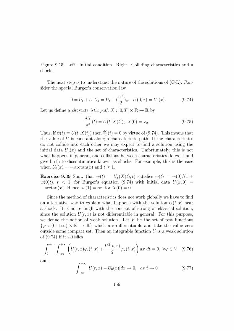
Figure 9.15: Left: Initial condition. Right: Colliding characteristics and ashock.

The next step is to understand the nature of the solutions of (C-L). Con-sider the special Burger’s conservation law

0 = Ut + U Ux = Ut + (U2

2)x, U(0, x) = U0(x). (9.74)

Let us define a characteristic path X : [0, T ]! R " R by

dX

dt(t) = U(t, X(t)), X(0) = x0. (9.75)

Thus, if 0(t) ( U(t, X(t)) then d*dt (t) = 0 by virtue of (9.74). This means that

the value of U is constant along a characteristic path. If the characteristicsdo not collide into each other we may expect to find a solution using theinitial data U0(x) and the set of characteristics. Unfortunately, this is notwhat happens in general, and collisions between characteristics do exist andgive birth to discontinuities known as shocks. For example, this is the casewhen U0(x) = $ arctan(x) and t ) 1.

Exercise 9.39 Show that w(t) = Ux(X(t), t) satisfies w(t) = w(0)/(1 +w(0)t), t < 1, for Burger’s equation (9.74) with initial data U(x, 0) =$ arctan(x). Hence, w(1) =-, for X(0) = 0.

Since the method of characteristics does not work globally we have to findan alternative way to explain what happens with the solution U(t, x) neara shock. It is not enough with the concept of strong or classical solution,since the solution U(t, x) is not di!erentiable in general. For this purpose,we define the notion of weak solution. Let V be the set of test functions{, : (0, +-) ! R " R} which are di!erentiable and take the value zerooutside some compact set. Then an integrable function U is a weak solutionof (9.74) if it satisfies

" +&

0

" +&

#&

:U(t, x),t(t, x) +

U2(t, x)

2,x(t, x)

;dx dt = 0, 4, # V (9.76)

and " +&

#&|U(t, x)$ U0(x)|dx" 0, as t" 0 (9.77)

156

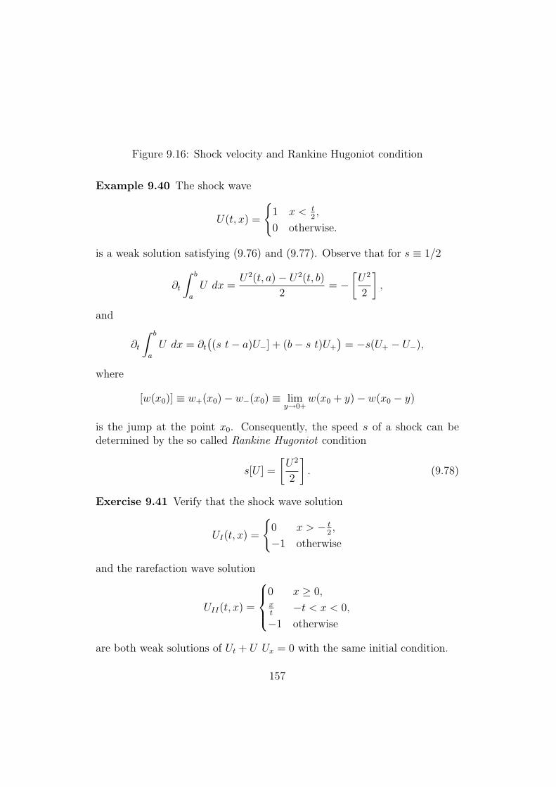
Figure 9.16: Shock velocity and Rankine Hugoniot condition

Example 9.40 The shock wave

U(t, x) =

/1 x < t

2 ,

0 otherwise.

is a weak solution satisfying (9.76) and (9.77). Observe that for s ( 1/2

"t

" b

a

U dx =U2(t, a)$ U2(t, b)

2= $

9U2

2

<,

and

"t

" b

a

U dx = "t

%(s t$ a)U#] + (b$ s t)U+

&= $s(U+ $ U#),

where

[w(x0)] ( w+(x0)$ w#(x0) ( limy%0+

w(x0 + y)$ w(x0 $ y)

is the jump at the point x0. Consequently, the speed s of a shock can bedetermined by the so called Rankine Hugoniot condition

s[U ] =

9U2

2

<. (9.78)

Exercise 9.41 Verify that the shock wave solution

UI(t, x) =

/0 x > $ t

2 ,

$1 otherwise

and the rarefaction wave solution

UII(t, x) =

283

84

0 x ) 0,xt $t < x < 0,

$1 otherwise

are both weak solutions of Ut + U Ux = 0 with the same initial condition.

157

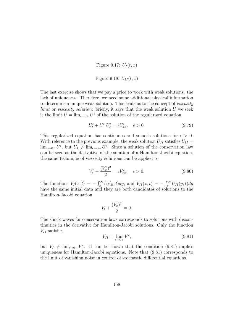
Figure 9.17: UI(t, x)

Figure 9.18: UII(t, x)

The last exercise shows that we pay a price to work with weak solutions: thelack of uniqueness. Therefore, we need some additional physical informationto determine a unique weak solution. This leads us to the concept of viscositylimit or viscosity solution: briefly, it says that the weak solution U we seekis the limit U = lim$%0+ U $ of the solution of the regularized equation

U $t + U $ U $

x = $U $xx, $ > 0. (9.79)

This regularized equation has continuous and smooth solutions for $ > 0.With reference to the previous example, the weak solution UII satisfies UII =lim$%0+ U $, but UI '= lim$%0+ U $. Since a solution of the conservation lawcan be seen as the derivative of the solution of a Hamilton-Jacobi equation,the same technique of viscosity solutions can be applied to

V $t +

(V $x )2

2= $V $

xx, $ > 0. (9.80)

The functions VI(x, t) = $$&

x UI(y, t)dy, and VII(x, t) = $$&

x UII(y, t)dyhave the same initial data and they are both candidates of solutions to theHamilton-Jacobi equation

Vt +(Vx)2

2= 0.

The shock waves for conservation laws corresponds to solutions with discon-tinuities in the derivative for Hamilton-Jacobi solutions. Only the functionVII satisfies

VII = lim$%0+

V $, (9.81)

but VI '= lim$%0+ V $. It can be shown that the condition (9.81) impliesuniqueness for Hamilton-Jacobi equations. Note that (9.81) corresponds tothe limit of vanishing noise in control of stochastic di!erential equations.

158

9.3.4 Numerical Approximations of Conservation Lawsand Hamilton-Jacobi Equations

We have seen that the viscous problem

"tu+ + "xH(u+) = 'u+

xx for (x, t) # R! (0, +-), (9.82)

u+(x, 0) = u0(x) for x # R,

can be used to construct unique solutions to the conservation law

"tu + "xH(u) = 0 for (x, t) # R! (0, +-), (9.83)

u(x, 0) = u0(x) for x # R.

In this section we will develop numerical approximations to the conservationlaw (9.83) and the related Hamilton-Jacobi equation

"tv + H("xv) = 0,

based on viscous approximations. We will also see that too little viscositymay give unstable approximations.

To show the di"culties to solve numerically a problem like (9.83) and(9.82) we consider a related steady-state problem (i.e. a problem that hasno dependence on t)

"xw(x)$ ' "2xw(x) = 0 for x < 0, (9.84)

limx%#&

w(x) = 1, w(0) = 0,

where ' ) 0 is fixed. It is easy to verify that the exact solution is w(x) =1 $ exp(x

+ ), for x * 0. Now, we construct a uniform partition of ($-, 0]with nodes xj = j#x for j = 0,$1,$2, . . ., where #x > 0 is a given meshsize. Denoting by Wj the approximation of w(xj), the use of a second orderaccurate finite element method or finite di!erence scheme method leads tothe scheme

Wj+1 $Wj#1

2#x$ '

Wj+1 $ 2Wj + Wj#1

(#x)2= 0, j = $N + 1, . . . ,$1,

W0 = 0, (9.85)

W#N = 1.

159

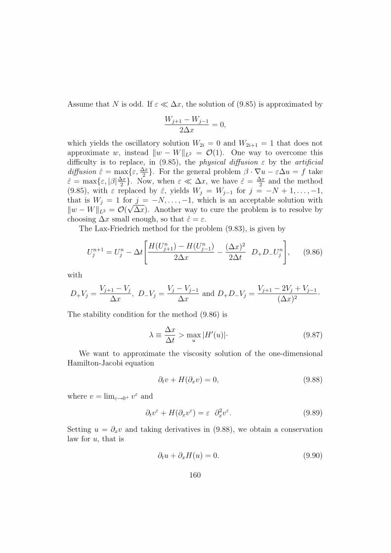
Assume that N is odd. If '6 #x, the solution of (9.85) is approximated by

Wj+1 $Wj#1

2#x= 0,

which yields the oscillatory solution W2i = 0 and W2i+1 = 1 that does notapproximate w, instead +w $ W+L2 = O(1). One way to overcome thisdi"culty is to replace, in (9.85), the physical di!usion ' by the artificialdi!usion ' = max{', !x

2 }. For the general problem % ·2u $ '#u = f take' = max{', |%|!x

2 }. Now, when ' 6 #x, we have ' = !x2 and the method

(9.85), with ' replaced by ', yields Wj = Wj#1 for j = $N + 1, . . . ,$1,that is Wj = 1 for j = $N, . . . ,$1, which is an acceptable solution with+w $W+L2 = O(

,#x). Another way to cure the problem is to resolve by

choosing #x small enough, so that ' = '.The Lax-Friedrich method for the problem (9.83), is given by

Un+1j = Un

j $#t

=H(Un

j+1)$H(Unj#1)

2#x$ (#x)2

2#tD+D#Un

j

>, (9.86)

with

D+Vj =Vj+1 $ Vj

#x, D#Vj =

Vj $ Vj#1

#xand D+D#Vj =

Vj+1 $ 2Vj + Vj#1

(#x)2·

The stability condition for the method (9.86) is

# ( #x

#t> max

u|H "(u)|· (9.87)

We want to approximate the viscosity solution of the one-dimensionalHamilton-Jacobi equation

"tv + H("xv) = 0, (9.88)

where v = lim+%0+ v+ and

"tv+ + H("xv

+) = ' "2xv

+. (9.89)

Setting u = "xv and taking derivatives in (9.88), we obtain a conservationlaw for u, that is

"tu + "xH(u) = 0. (9.90)

160

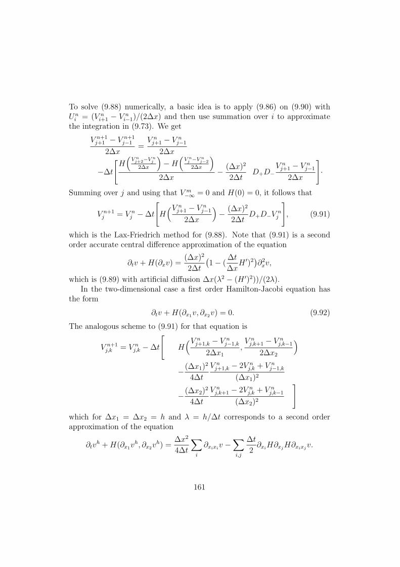
To solve (9.88) numerically, a basic idea is to apply (9.86) on (9.90) withUn

i = (V ni+1 $ V n

i#1)/(2#x) and then use summation over i to approximatethe integration in (9.73). We get

V n+1j+1 $ V n+1

j#1

2#x=

V nj+1 $ V n

j#1

2#x

$#t

=H

!V n

j+2#V nj

2!x

#$H

!V n

j #V nj#2

2!x

#

2#x$ (#x)2

2#tD+D#

V nj+1 $ V n

j#1

2#x

>·

Summing over j and using that V m#& = 0 and H(0) = 0, it follows that

V n+1j = V n

j $#t

=H

!V nj+1 $ V n

j#1

2#x

#$ (#x)2

2#tD+D#V n

j

>, (9.91)

which is the Lax-Friedrich method for (9.88). Note that (9.91) is a secondorder accurate central di!erence approximation of the equation

"tv + H("xv) =(#x)2

2#t

%1$ (

#t

#xH ")2

&"2

xv,

which is (9.89) with artificial di!usion #x(#2 $ (H ")2))/(2#).In the two-dimensional case a first order Hamilton-Jacobi equation has

the form

"tv + H("x1v, "x2v) = 0. (9.92)

The analogous scheme to (9.91) for that equation is

V n+1j,k = V n

j,k $#t

=H

!V nj+1,k $ V n

j#1,k

2#x1,V n

j,k+1 $ V nj,k#1

2#x2

#

$(#x1)2

4#t

V nj+1,k $ 2V n

j,k + V nj#1,k

(#x1)2

$(#x2)2

4#t

V nj,k+1 $ 2V n

j,k + V nj,k#1

(#x2)2

>

which for #x1 = #x2 = h and # = h/#t corresponds to a second orderapproximation of the equation

"tvh + H("x1v

h, "x2vh) =

#x2

4#t

,

i

"xixiv $,

i,j

#t

2"xiH"xjH"xixjv.

161