chapter 9 channel capacity and coding
TRANSCRIPT

Introduction to Communications Prof. Jae Hong Lee, SNU Chapter 9. Channel Capacity and Coding - 1 - 1st Semester, 2008
Chapter 9 Channel Capacity and Coding
Text. [1] J. G. Proakis and M. Salehi, Communication Systems Engineering, 2/e. Prentice Hall, 2002.
9.1 Modeling of Communication Channels
9.2 Channel Capacity
9.3 Bounds on Communication (partly skipped)
9.4 Coding for Reliable Communication (skipped)
9.5 Linear Block Codes (partly covered)
9.6 Cyclic Codes (skipped)
9.7 Convolutional Codes (partly covered)
9.8 Complex Codes Based on Combination of Simple Codes
9.9 Coding for Bandwidth-Constrained Channels
9.10 Practical Applications of Coding
The goal of any communication system is to transmit information from an information source to a
destination via a communication channel.

Introduction to Communications Prof. Jae Hong Lee, SNU Chapter 9. Channel Capacity and Coding - 2 - 1st Semester, 2008
9.1 Modeling of Communication Channels
A communication channel is a medium over which information can be transmitted or in which information can
be stored, such as coaxial cables, ionospheric propagation, free space, fiber optic cables, and magnetic and
optical disks.
They accept a signal at their inputs and deliver a signal at their outputs at another location (in case of
transmission) or at a later time (in case of storage).
The output of a communication channel becomes different from its input due to various factors such as
attenuation, nonlinearities, bandwidth limitations, multipath propagation, and noise.
Due to the presence of noise and fading, the input-output relation in a communication channel is, generally,
a stochastic relation.
A waveform channels accepts a (continuous-time) waveform signal as its input and produce a waveform
signal as its output.

Introduction to Communications Prof. Jae Hong Lee, SNU Chapter 9. Channel Capacity and Coding - 3 - 1st Semester, 2008
Because the bandwidth of any practical channel is limited, a waveform channel becomes equivalent to a
discrete-time channel by using the sampling theorem.
In a discrete-time channel, both input and output are discrete-time signals.
In a discrete-time channel, the channel is called a discrete channel if the values that the input and output
variables can take are finite or countably infinite.
In general, a discrete channel is defined by the input alphabet X , the output alphabet y , and the
conditional PMF ( | )p y x of the output sequence given the input sequence.
A schematic representation of a discrete channel is shown in Figure 9.1.

Introduction to Communications Prof. Jae Hong Lee, SNU Chapter 9. Channel Capacity and Coding - 4 - 1st Semester, 2008
Figure 9.1 A discrete channel.

Introduction to Communications Prof. Jae Hong Lee, SNU Chapter 9. Channel Capacity and Coding - 5 - 1st Semester, 2008
In general, the output iy does not only depend on the input at the same time ix but also on the previous
inputs (channels with ISI, see Chapter 8), or even previous and future inputs (in storage channels).
In this case, we say that the channel has memory.
For a discrete-memoryless channel, for any n∈y y and n∈x X , we have
1
( | ) ( | )n
i ii
p p y x=
=∏y x (9.1.1)
where ( | )i ip y x is transition probability.
All channel models that we will discuss in this chapter are memoryless.
A special case of a discrete-memoryless channel is the binary-symmetric channel (BSC).
Figure 9.2 shows a binary-symmetric channel.
In a binary-symmetric channel, (0 |1) (1| 0)P P= = ε is called the crossover probability.

Introduction to Communications Prof. Jae Hong Lee, SNU Chapter 9. Channel Capacity and Coding - 6 - 1st Semester, 2008
Figure 9.2 Binary-symmetric channel (BSC).

Introduction to Communications Prof. Jae Hong Lee, SNU Chapter 9. Channel Capacity and Coding - 7 - 1st Semester, 2008
Ex. 9.1.1
Consider an additive white Gaussian noise channel with binary antipodal signaling.
The error probability of a 1 being detected as 0 or a 0 being detected as 1 is given by
(1| 0)P=ε
(0 |1)P=
0
2 bQNε⎛ ⎞
= ⎜ ⎟⎜ ⎟⎝ ⎠
(9.1.2)
where 0N is the (single-sided) noise power spectral density and bε is the bit energy of each of the antipodal
signals representing 0 and 1.
This discrete channel is a binary symmetric channel.
Ex. 9.1.2
In an AWGN channel with binary antipodal signaling, the input is either bε or bε− .
The output is the sum of the input and the Gaussian noise.

Introduction to Communications Prof. Jae Hong Lee, SNU Chapter 9. Channel Capacity and Coding - 8 - 1st Semester, 2008
For this binary-input, continuous-output channel, we have { }bε= ±X and =y and 2
2( )
22
1( | )2
y x
f y x e σ
πσ
−−
=
where 2σ is the variance of the noise.
Ex.
As an example of a continuous-amplitude channel, consider the discrete-time additive white Gaussian noise
channel with an input power constraint.
In this channel, both the input alphabet X and output alphabet y are the set of real numbers.
If the channel input is X , the channel output is given by
Y Z= + (9.1.3)
where Z is the Gaussian noise in the channel with mean 0 and variance NP .
Assume that inputs to this channel satisfy power constraint such that,
for large n , an input block of length n satisfies

Introduction to Communications Prof. Jae Hong Lee, SNU Chapter 9. Channel Capacity and Coding - 9 - 1st Semester, 2008
2
1
1 n
ii
x Pn =
≤∑ (9.1.4)
where P is some fixed power constraint.
This channel model is shown in Figure 9.3.
Figure 9.3 Additive white Gaussian noise channel power constraint.

Introduction to Communications Prof. Jae Hong Lee, SNU Chapter 9. Channel Capacity and Coding - 10 - 1st Semester, 2008
9.2 Channel Capacity
The reliability of transmitting information over any communication channel is measured by the probability of
correct reception at the receiver.
By the noisy channel-coding theorem by Shannon (1948), reliable transmission (that is transmission with
error probability less any given value) is possible even over a noisy channel as long as the transmission rate is
less than some number called the channel capacity.
This implies that the basic limitation that noise causes in a communication channel is not on the
reliability of communication, but on the speed of communication.
Figure 9.4 shows an example of a discrete-memoryless channel with four inputs and outputs.

Introduction to Communications Prof. Jae Hong Lee, SNU Chapter 9. Channel Capacity and Coding - 11 - 1st Semester, 2008
Figure 9.4 Example of a discrete channel.

Introduction to Communications Prof. Jae Hong Lee, SNU Chapter 9. Channel Capacity and Coding - 12 - 1st Semester, 2008
Since the receiver does not know whether a or d was transmitted if it receives a ;
the receiver does not know whether a or b was transmitted if it receives b , etc.;
there always exists a possibility of error.
But if the transmitter and receiver agree that the transmitter only uses letters a and c , then there exists no
ambiguity.
In this case, if the receiver receives a or b it knows that a was transmitted; and if it receives c or d
it knows that c was transmitted.
This means that the two symbols a and c can be transmitted over this channel without error; that is,
errors can be avoided by using only a subset of all possible inputs whose corresponding possible outputs are
disjoint in this example.
The inputs in the chosen subset of possible inputs should be “far apart” such that their “images” under the
channel operation are nonoverlapping (or have negligible overlaps).
Notice that there is no way to have nonoverlapping outputs for a binary symmetric channel.

Introduction to Communications Prof. Jae Hong Lee, SNU Chapter 9. Channel Capacity and Coding - 13 - 1st Semester, 2008
In order to use the results of the above argument for the binary symmetric channel, we need to apply it not
to the channel itself, but to the extension channel.
The n th extension of a channel with input alphabet X , output alphabets alphabet y , and conditional
probabilities ( | )P y x is a channel with input and output alphabets nX and ny and conditional probability
1
( | ) ( | )n
i ii
P P y x=
=∏y x .
The n th extension of a binary symmetric channel takes binary sequences of length n as its input and
output which is shown in Figure 9.5.

Introduction to Communications Prof. Jae Hong Lee, SNU Chapter 9. Channel Capacity and Coding - 14 - 1st Semester, 2008
Figure 9.5 n th extension of a binary symmetric channel.

Introduction to Communications Prof. Jae Hong Lee, SNU Chapter 9. Channel Capacity and Coding - 15 - 1st Semester, 2008
By the law of large numbers (see Chapter 4), for n large enough, if a binary sequence of length n is
transmitted over the channel, the output will disagree with the input with high probability at nε positions.
The number of possible sequences that disagree with a sequence of length n at nε positions is given by
nn⎛ ⎞⎜ ⎟⎝ ⎠ε
.
By using Stirling’s approximation ! 2n nn n e nπ−≈ , we obtain
( )2 bnHnn⎛ ⎞
≈⎜ ⎟⎝ ⎠
ε
ε (9.2.1)
where 2 2( ) log (1 )log (1 )bH = − − − −ε ε ε ε ε is the binary entropy function (see Chapter 6).
This means that, for any input sequence of length n , there exist roughly ( )2 bnH ε highly probable
corresponding output sequences.
On the other hand, the total number of highly probable output sequences is roughly ( )2nH Y .

Introduction to Communications Prof. Jae Hong Lee, SNU Chapter 9. Channel Capacity and Coding - 16 - 1st Semester, 2008
Therefore, the maximum number of input sequences that produce almost nonoverlapping output sequences,
is at most equal to ( )
( )22 b
nH Y
nHM = ε
( )( ) ( )2 bn H Y H−= ε (9.2.2)
and the transmission rate per channel use is given by
log MRn
=
( ) ( )bH Y H= − ε . (9.2.3)
Note that ε depends on the channel and we cannot control it.
However, the probability distribution of the random variable Y depends both on the input distribution
( )p x and the channel properties characterized by ε .
Figure 9.6 gives a schematic representation of this case.

Introduction to Communications Prof. Jae Hong Lee, SNU Chapter 9. Channel Capacity and Coding - 17 - 1st Semester, 2008
Figure 9.6 Schematic representation of a BSC.

Introduction to Communications Prof. Jae Hong Lee, SNU Chapter 9. Channel Capacity and Coding - 18 - 1st Semester, 2008
To maximize the transmission rate over the channel, one has to choose ( )p x that maximizes ( )H Y .
If X is chosen to be a uniformly distributed random variable, that is, ( 0) ( 1) 0.5P X P X= = = = , then Y
is uniformly distributed and ( )H Y is maximized.
Since the maximum value of ( )H Y is 1, from (9.2.3) the maximum of the transmission rate is given by
1 ( )bR H= − ε . (9.2.4)
It can be proved that the above rate is the maximum rate at which reliable transmission over the BSC is
possible.
By reliable transmission we mean that the error probability can be made to tend to 0 as the sequence
length n tends to infinity.
The channel capacity in this case is shown in Figure 9.7.

Introduction to Communications Prof. Jae Hong Lee, SNU Chapter 9. Channel Capacity and Coding - 19 - 1st Semester, 2008

Introduction to Communications Prof. Jae Hong Lee, SNU Chapter 9. Channel Capacity and Coding - 20 - 1st Semester, 2008
Note that the both cases with 0=ε and 1=ε result in a perfect channel having channel capapcity 1C = .
This means that a channel that always flips the input is as good as the channel that transmits the input
without error.
The worst case happens when the channel flips the input with probability 12
which leads to a useless
channel having channel capacity 0C = .
The maximum rate at which one can communicate over a discrete-memoryless channel and still make the
error probability to approach 0 as the code block length increases, is called the channel capacity which is
denoted by C .
Theorem 9.2.1 [Noisy Channel-Coding Theorem]
The capacity of a discrete-memoryless channel is given by
( )max ( ; )
p xC I X Y= (9.2.5)
where ( ; )I X Y is the mutual information between the channel input X and the channel output Y (see

Introduction to Communications Prof. Jae Hong Lee, SNU Chapter 9. Channel Capacity and Coding - 21 - 1st Semester, 2008
Chapter 6).
Definition 6.4.1
The mutual information between two discrete random variables X and Y is denoted by ( );I X Y and
defined by
( ) ( ) ( );I X Y H X H X Y= − . (6.4.1)
If the transmission rate R is less than C , then for any 0δ > there exists a code with block length n
large enough whose error probability is less than δ .
If R C> , the error probability of any code with any block length is bounded away from 0 .
According to this theorem, any communication channel is characterized by a number called capacity that
determines how much information can be transmitted over it, regardless of all other properties.
Therefore, to compare two channels from an information transmission point of view, it is enough to
compare their capacities.
Introduction to Communications Prof. Jae Hong Lee, SNU Chapter 9. Channel Capacity and Coding - 22 - 1st Semester, 2008
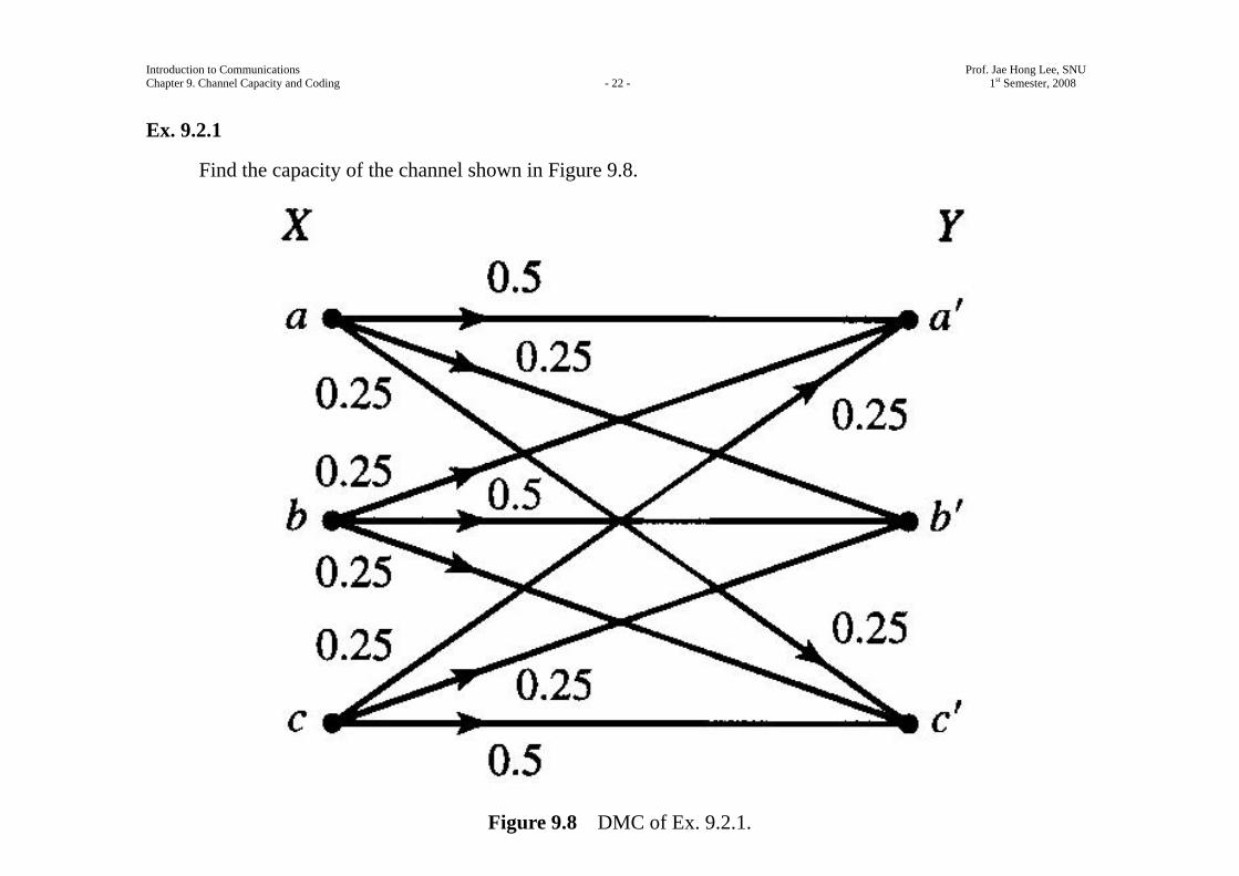
Ex. 9.2.1
Find the capacity of the channel shown in Figure 9.8.
Figure 9.8 DMC of Ex. 9.2.1.

Introduction to Communications Prof. Jae Hong Lee, SNU Chapter 9. Channel Capacity and Coding - 23 - 1st Semester, 2008
Solution
We have ( ; ) ( ) ( | )I X Y H Y H Y X= − .
But
( | ) ( ) ( | ) ( ) ( | ) ( ) ( | )H Y X P X a H Y X a P X b H Y X b P X c H Y X c= = = + = = + = = .
From Figure 9.8, for all three cases of X a= , X b= , and X c= , the random variable Y is ternary with
probabilities 0.25 , 0.25 , and 0.5 .
Therefore,
( | ) ( | )H Y X a H Y X b= = =
( | )H Y X c= =
1.5= .
Because ( ) ( ) ( ) 1P X a P X b P X c= + = + = = ,
we have
( | ) 1.5H Y X =
and
Introduction to Communications Prof. Jae Hong Lee, SNU Chapter 9. Channel Capacity and Coding - 24 - 1st Semester, 2008
( ; ) ( ) ( | )I X Y H Y H Y X= −
( ) 1.5H Y= − .
To maximize ( ; )I X Y , it needs to maximize ( )H Y , which is maximized when the random variable Y is
equiprobable.
It is not clear in general if there exists an input distribution that results in a uniform distribution on the
output.
However, in this special case (due to the symmetry of the channel) a uniform input distribution results in a
uniform output distribution and
2( ) log 3H Y =
1.585= (bits).
Hence, the capacity of this channel is given by
( )max ( ; )
p xC I X Y=
( ) ( | )H Y H Y X= −
1.585 1.5= − 0.085= bits/transmission.

Introduction to Communications Prof. Jae Hong Lee, SNU Chapter 9. Channel Capacity and Coding - 25 - 1st Semester, 2008
9.2.1 Gaussian Chanel Capacity
A discrete-time Gaussian channel with input power constraint is characterized by the input-output relation
Y X Z= + (9.2.6)
where Z is a zero-mean Gaussian random variable with variance NP , and an input power constraint that
2
1
1 n
ii
x Pn =
≤∑ (9.2.7)
applies to any input sequence of length n for n large enough.
For blocks of length n at the input, output, and noise, we have
= +y x z . (9.2.8)
By the law of large numbers, if n is large, we have
2 2
1 1
1 1 ( )n n
i i ii i
z y xn n= =
= −∑ ∑
NP≤ (9.2.9)
or 2|| || Nn P− ≤y x . (9.2.10)

Introduction to Communications Prof. Jae Hong Lee, SNU Chapter 9. Channel Capacity and Coding - 26 - 1st Semester, 2008
This means that, with probability approaching 1 (as n increases), y will be located within an n -
dimensional sphere (hypersphere) of radius NnP centered at x .
On the other hand, due to the power constraint of P on the input and the independence of the input and
noise, the output power is the sum of the input power and the noise power, that is,
2 2
1 1
1 1 ( )n n
i i ii i
y x zn n= =
= +∑ ∑
2 2
1
1 ( )n
i ii
x zn =
= +∑
NP P≤ + (9.2.11)
or 2|| || ( )Nn P P≤ +y . (9.2.12)
This implies that the output sequences (again, asymptotically and with high probability) will be located
within an n -dimensional hypersphere of radius ( )Nn P P+ centered at the origin.
Figure 9.9 shows the sequences in the output space.

Introduction to Communications Prof. Jae Hong Lee, SNU Chapter 9. Channel Capacity and Coding - 27 - 1st Semester, 2008

Introduction to Communications Prof. Jae Hong Lee, SNU Chapter 9. Channel Capacity and Coding - 28 - 1st Semester, 2008
Now the question is: how many x sequences can we transmit over this channel such that the hyperspheres
corresponding to these sequences do not overlap in the output space?
An equivalent question is: how many hyperspheres of radius NnP can we pack in the hypersphere of
radius ( )Nn P P+ ?
The answer is roughly the ratio of the volumes of the two hyperspheres.
Let the volume of an n -dimensional hypersphere is given by n
n nV K R= (9.2.13)
where R is the radius of the hypersphere and nK is a constant independent of R .
Then, the number of messages that can be reliably transmitted over this channel is given by
( )2
2
( )
( )
n
n Nn
n N
K n P PM
K nP
+=
2n
N
N
P PP
⎛ ⎞+= ⎜ ⎟⎝ ⎠

Introduction to Communications Prof. Jae Hong Lee, SNU Chapter 9. Channel Capacity and Coding - 29 - 1st Semester, 2008
21
n
N
PP
⎛ ⎞= +⎜ ⎟⎝ ⎠
. (9.2.14)
Therefore, the capacity of a discrete-time additive white Gaussian noise channel with input power constraint
P is given by
21 logC Mn
=
21 log 1
2 N
n Pn P
⎛ ⎞= ⋅ +⎜ ⎟
⎝ ⎠
21 log 12 N
PP
⎛ ⎞= +⎜ ⎟
⎝ ⎠ bits/transmission . (9.2.15)
We can sample a continuous-time, bandlimited, additive white Gaussian noise channel with noise power
spectral density 0
2N , input power constraint P , and bandwidth W at the Nyquist rate to obtain a discrete-
time channel.

Introduction to Communications Prof. Jae Hong Lee, SNU Chapter 9. Channel Capacity and Coding - 30 - 1st Semester, 2008
Then, the power per sample becomes P and the noise power per sample is given by
0
2W
N W
NP df+
−= ∫
0WN= .
Substituting these results into (9.2.15), we obtain
20
1 log 1 bits/transmission2
PCN W
⎛ ⎞= +⎜ ⎟
⎝ ⎠. (9.2.16)
If we multiply this result by the number of transmissions/sec, which is 2W , we obtain the channel capacity
20
log 1 bits/secPC WN W
⎛ ⎞= +⎜ ⎟
⎝ ⎠. (9.2.17)
Ex. 9.2.2
Find the capacity of a telephone channel with bandwidth 3000W = Hz and SNR of 39 dB.
Solution
The SNR of 39 dB is equivalent to 7943.

Introduction to Communications Prof. Jae Hong Lee, SNU Chapter 9. Channel Capacity and Coding - 31 - 1st Semester, 2008
Using Shannon’s relation in (9.2.17) we have
20
log 1 PC WN W
⎛ ⎞= +⎜ ⎟
⎝ ⎠
23000 log (1 7943)= +
38,867 bits/sec≈ .
9.3 Bounds on Communication
There exists a trade-off between signal power P and bandwidth W in the sense that one can compensate for
the other.
Increasing the input signal power increases the channel capacity, because when one has more power to
spend, one can choose a larger number of input levels which are far apart and, hence, more information
bits/transmission are possible.
However, the increase in capacity as a function of power is logarithmic and slow.

Introduction to Communications Prof. Jae Hong Lee, SNU Chapter 9. Channel Capacity and Coding - 32 - 1st Semester, 2008
This is because if one is transmitting with a certain number of input levels that are Δ apart to allow a
certain level of immunity against noise and wants to increase the number of input levels,
one has to introduce new levels with amplitudes higher than the existing levels, and this requires a lot of power.
Nevertheless, the capacity of the channel can be increased to any value by increasing the input power.
Increasing channel bandwidth W has two contrasting effects.
On one hand, on a larger bandwidth channel one can transmit more samples/sec and, therefore, increase the
transmission rate.
On the other hand, a larger bandwidth means a larger input noise to the receiver and this degrades the
performance of the channel.
These effects are seen from the two W ’s which appear in (9.2.17).

Introduction to Communications Prof. Jae Hong Lee, SNU Chapter 9. Channel Capacity and Coding - 33 - 1st Semester, 2008
Applying L’Hospital’s rule to (9.2.17), we obtain
0
lim logW
PC eN→∞
=
0
1.44 PN
= (9.3.1)
which implies that by increasing the bandwidth alone the capacity is not increased to any desired value,
contrary to the case of power.
Figure 9.10 shows the channel capacity C versus bandwidth W .

Introduction to Communications Prof. Jae Hong Lee, SNU Chapter 9. Channel Capacity and Coding - 34 - 1st Semester, 2008
Figure 9.10 Channel capacity versus bandwidth.

Introduction to Communications Prof. Jae Hong Lee, SNU Chapter 9. Channel Capacity and Coding - 35 - 1st Semester, 2008
In any practical communication system, we must have R C< .
If an AWGN channel is employed, we have
0
log 1 PR WN W
⎛ ⎞< +⎜ ⎟
⎝ ⎠. (9.3.2)
By dividing both sides by W and defining the spectral bit rate RrW
= , we obtain
0
log 1 PrN W
⎛ ⎞< +⎜ ⎟
⎝ ⎠. (9.3.3)
The energy per bit is given by bPR
ε = .
By substituting this into (9.3.3), we obtain
0
log 1 br rNε⎛ ⎞
< +⎜ ⎟⎝ ⎠
(9.3.4)
or, equivalently,

Introduction to Communications Prof. Jae Hong Lee, SNU Chapter 9. Channel Capacity and Coding - 36 - 1st Semester, 2008
0
2 1rb
N rε −
> . (9.3.5)
Figure 9.11 shows the spectral bit rate r versus 0
b
Nε .
In Figure 9.11, the curve is given by
0
log 1 br rNε⎛ ⎞
= +⎜ ⎟⎝ ⎠
(9.3.6)
which divides the plane into two regions.
In the region below the curve, reliable communication is possible; and
in the region above the curve, reliable communication is not possible

Introduction to Communications Prof. Jae Hong Lee, SNU Chapter 9. Channel Capacity and Coding - 37 - 1st Semester, 2008

Introduction to Communications Prof. Jae Hong Lee, SNU Chapter 9. Channel Capacity and Coding - 38 - 1st Semester, 2008
The performance of any communication system can be marked by a point in Figure 9.11 and the closer the
point is to the curve, the closer is the performance of the system to that of an optimal system.
From this curve, it is seen that (as r tends to 0 ),
0
ln 2b
Nε
=
0.693=
1.6dB−∼ (9.3.7)
is an absolute minimum which is needed for reliable communication.
In other words, for reliable communication, we must have
0
0.693b
Nε
> . (9.3.8)
In Figure 9.11, if the spectral bit rate 1r << , the channel bandwidth is large and the main concern is
limitation on power.
This case is usually referred to as the power-limited case.

Introduction to Communications Prof. Jae Hong Lee, SNU Chapter 9. Channel Capacity and Coding - 39 - 1st Semester, 2008
Signaling schemes with high dimensionality such as orthogonal, biorthogonal, and simplex are used in this
case.
If the spectral bit rate 1r >> , the channel bandwidth is small and, therefore, it is referred to as the
bandwidth-limited case.
Signaling schemes with low dimensionality (that is, with crowded constellations) such as 256 -QAM are
used in this case.
Entropy gives a lower bound on the rate of the codes that are capable of reproducing the source output with
no error, and the rate-distortion function gives a lower bound on the rate of the source with no error, and the
rate-distortion function gives a lower bound on the rate of the codes capable of reproducing the source with
distortion D .
If we want to transmit a source U reliably via a channel with capacity C , we require that
( )H U C< . (9.3.9)

Introduction to Communications Prof. Jae Hong Lee, SNU Chapter 9. Channel Capacity and Coding - 40 - 1st Semester, 2008
If transmission with a maximum distortion equal to D is desired, then the condition is given by
( )R D C< . (9.3.10)
These two relations define fundamental limits on the transmission of information.
In both cases, we have assumed that one transmission over the channel is possible for each source output.
Ex. 9.3.1
A zero-mean Gaussian source with power-spectral density
( )20,000X
fS f ⎛ ⎞= Π⎜ ⎟⎝ ⎠
is to be transmitted via a telephone channel described in Example 9.2.2.
Find the minimum distortion achievable if mean-squared distortion is used.
Solution
The bandwidth of the source is 10,000 Hz, and hencee, it can be sampled at a rate of 20,000 samples/sec.

Introduction to Communications Prof. Jae Hong Lee, SNU Chapter 9. Channel Capacity and Coding - 41 - 1st Semester, 2008
The power of the source is given by
( )X XP S f df∞
−∞= ∫
20,000=
The variance of each sample is given by 2 20,000σ =
and the rate distortion function for 20,000D < is given by 21( ) log
2R D
Dσ
=
1 20,000log bits/sample2 D
=
which is equivalent to
20,000( ) 10,000log bits/secR DD
= .
Since the capacity of the channel (derived in Example 9.2.2) ( )R D is 38,867 bits/sec, we can derive the
least possible distortion by solving
20,00038,867 10,000logD
=

Introduction to Communications Prof. Jae Hong Lee, SNU Chapter 9. Channel Capacity and Coding - 42 - 1st Semester, 2008
for D , which results in 1352D = .
In general, it can be shown that the rate-distortion function for a waveform Gaussian source with power-
spectral density
, | | ,( )
0, otherwise,S
X
A f WS f
<⎧= ⎨⎩
(9.3.11)
and with distortion measure
( ) 22
2
1( ), ( ) lim [ ( ) ( )]T
TTd u t v t u t v t dt
T→∞ −= −∫ (9.3.12)
is given by
2log , 2 ,( )
0, 2 .
SS S
S
AWW D AWR D D
D AW
⎧ ⎛ ⎞ <⎪ ⎜ ⎟= ⎝ ⎠⎨⎪ ≥⎩
(9.3.13)
If this source is to be transmitted via an additive white Gaussian noise channel with bandwidth cW , power
P , and noise-spectral density 0N , the minimum achievable distortion is obtained by solving the equation
0
2log 1 log Sc S
c
P AWW WN W D
⎛ ⎞ ⎛ ⎞+ =⎜ ⎟ ⎜ ⎟⎝ ⎠⎝ ⎠
. (9.3.14)

Introduction to Communications Prof. Jae Hong Lee, SNU Chapter 9. Channel Capacity and Coding - 43 - 1st Semester, 2008
From (9.3.14), we obtain
0
2 1c
S
WW
Sc
PD AWN W
−⎛ ⎞
= +⎜ ⎟⎝ ⎠
. (9.3.15)
It is seen that, in an optimal system, distortion decreases exponentially as c
S
WW
increases.
The ratio c
S
WW
is called the bandwidth-expansion factor.
We can also find the SQNR as
2SQNR SAWD
=
0
1c
S
WW
c
PN W
⎛ ⎞= +⎜ ⎟⎝ ⎠
(9.3.16)
In an optimal system, the final signal-to-noise (distortion) ratio increases exponentially with the bandwidth
expansion factor.

Introduction to Communications Prof. Jae Hong Lee, SNU Chapter 9. Channel Capacity and Coding - 44 - 1st Semester, 2008
9.3.1 Transmission of Analog Sources by PCM (skipped)
PCM is one of the most commonly used schemes for transmission of analog data.
In a PCM system the quantization noise (distortion) is given by [Section 6.6] 2
2 max[ ]3 4v
xE X =⋅
where maxx is the maximum input amplitude and v is the number of bits/sample.
If the source bandwidth is sW , then the sampling frequency in an optimal system is 2s sf W= , and the bit
rate is 2 sR vW= .
Assuming that the binary data is directly transmitted over the channel, the minimum channel bandwidth that
can accommodate this bit rate [Nyquist criterion, see Chapter 8] is given by
2cRW =
sv W= . (9.3.17)
Therefore, the quantization noise is given by

Introduction to Communications Prof. Jae Hong Lee, SNU Chapter 9. Channel Capacity and Coding - 45 - 1st Semester, 2008
22 max[ ]
3 4c
s
WW
xE X =
⋅
. (9.3.18)
If the output of a PVM system is transmitted over a noisy channel with error probability bP , some bits will
be received in error and another type of distortion, due to transmission, will also be introduced.
This distortion will be independent from the quantization distortion and since the quantization error is zero
mean, the total distortion will be the sum of these distortions [see Section 4.3.2].
Assume that bP is small enough such that in a block of length v , either no error or one error can occur.
This one error can occur at any of the v locations and, therefore, its contribution to the total distortion
varies accordingly.
If an error occurs in the least significant bit, it results in a change of Δ in the output level;
if it happens in the next bit, it results in 2Δ change in the output; and
if it occurs at the most significant bit, it causes a level change equal to 12v− Δ at the output.

Introduction to Communications Prof. Jae Hong Lee, SNU Chapter 9. Channel Capacity and Coding - 46 - 1st Semester, 2008
Assuming these are the only possible errors, the transmission distortion is obtained as
2 1 2
1[ ] (2 )
vi
T bi
E D P −
=
= Δ∑
2 4 13
c
s
WW
bP −= Δ (9.3.19)
and the total distortion is given by
22max
total4 1
33 4
c
s
c
s
WW
bWW
xD P −= + Δ
⋅
. (9.3.20)
Note that
max22v
xΔ =
max
2 1v
x=
−. (9.3.21)
Substituting for Δ , and assuming 4 1v , (9.3.20) is simplified to 2max
total (4 4 )3
c
s
WW
bxD P
−
≈ + . (9.3.22)

Introduction to Communications Prof. Jae Hong Lee, SNU Chapter 9. Channel Capacity and Coding - 47 - 1st Semester, 2008
The signal-to-noise (distortion) ratio at the receiving end is given by 2
2max
3SNR(4 4 )
c
s
WW
b
X
x P−
=
+
. (9.3.23)
bP depends on the modulation scheme employed to transmit the outputs of the PCM system.
If binary antipodal signaling is employed is employed, then
0
2 bbP Q
Nε⎛ ⎞
= ⎜ ⎟⎜ ⎟⎝ ⎠
(9.3.24)
and if binary orthogonal signaling with coherent detection is used, then
0
bbP Q
Nε⎛ ⎞
= ⎜ ⎟⎜ ⎟⎝ ⎠
. (9.3.25)
In (9.3.23), it is seen that for small bP , the SNR grows almost exponentially with c
s
WW
, the bandwidth-
expansion factor, and in this sense, a PCM system uses the available bandwidth efficiently.
Recall from Section 5.3, that another frequently used system that trades bandwidth for noise immunity is an

Introduction to Communications Prof. Jae Hong Lee, SNU Chapter 9. Channel Capacity and Coding - 48 - 1st Semester, 2008
FM system.
However, the SNR of an FM system is a quadratic function of the bandwidth-expansion factor [see (5.3.26)]
and, therefore, an FM system is not as bandwidth efficient as a PCM system.
9.4 Coding for Reliable Communication (skipped)
In Chapter 7, it was shown that both in baseband and carrier-modulation schemes, the error probability is a
function of the distance between the points in the signal constellation.
In fact, for binary equiprobable signals the error probability can be expressed as [see (7.6.10)]
12
02edP Q
N
⎛ ⎞= ⎜ ⎟⎜ ⎟
⎝ ⎠ (9.4.1)
where 12d is the Euclidean distance between 1( )s t and 2( )s t , given by
2 212 1 2[ ( ) ( )]d s t s t dt
∞
−∞= −∫ . (9.4.2)

Introduction to Communications Prof. Jae Hong Lee, SNU Chapter 9. Channel Capacity and Coding - 49 - 1st Semester, 2008
On the other hand, antipodal signaling with coherent demodulation performs best and has a Euclidean
distance 12 2 bd ε= .
Therefore,
0
2 beP Q
Nε⎛ ⎞
= ⎜ ⎟⎜ ⎟⎝ ⎠
. (9.4.3)
From the above, it is seen that to decrease the error probability, one has to increase the signal energy.
Increasing the signal energy can be done in two ways: 1) increasing the transmitter power 2) increasing the
transmission duration.
Increasing the transmitter power is not always feasible because each transmitter has a limitation on its
average power.
Increasing the transmission duration, in turn, decreases the transmission rate and, therefore, it seems that the
only way to make the error probability vanish is to let the transmission rate vanish.

Introduction to Communications Prof. Jae Hong Lee, SNU Chapter 9. Channel Capacity and Coding - 50 - 1st Semester, 2008
In fact, this was the communication engineers’ viewpoint in the pre-Shannon era.
By employing orthogonal signals, one can achieve reliable transmission at nonzero rate, as long as
0
2ln 2b
Nε
> (see Chapter 7).
Here, we show that 0
ln 2b
Nε
> is sufficient to achieve reliable transmission.
Note that this is the same condition which guarantees reliable transmission over an additive white Gaussian
noise channel when the bandwidth goes to infinity (see Figure 9.11 and (9.3.7)).
<Skipped.>
Comparing the two bounds, it is concluded that coding results in a power gain equivalent to
coding minH
cG d R= (9.4.55)
which is called the asymptotic-coding gain, or simply, the coding gain.
The coding gain is a function of two main code parameters, the minimum Hamming distance and the code

Introduction to Communications Prof. Jae Hong Lee, SNU Chapter 9. Channel Capacity and Coding - 51 - 1st Semester, 2008
rate.
Note that in general, 1cR < and , min 1Hd ≥ and, therefore, the coding gain can be greater or less than one.†
There exist many codes that can provide good coding gains.
For a given n and k the best code is the code that can provide the highest minimum Hamming distance.
To study the bandwidth requirements of coding, we observe that when no coding is used, the width of the
pulses employed to transmit one bit is given by
1bT
R= . (9.4.56)
After using coding, in the same time duration that k pulses were transmitted, we must now transmit n
pulses, which means that the duration of each pulse is reduced by a factor of ck Rn= .
† Although in a very bad code design we can even have , min 0Hd = , we will ignore such cases.

Introduction to Communications Prof. Jae Hong Lee, SNU Chapter 9. Channel Capacity and Coding - 52 - 1st Semester, 2008
Therefore, the bandwidth-expansion ratio is given by
coding
no coding
WB
W=
1
cR=
nk
= (9.4.57)
which implies that the bandwidth has increased linearly.
It can be proved that, in an AWGN channel, there exists a sequence of codes with parameters ( , )i in k with
fixed rate ( ic
i
k Rn= independent of i ) satisfying
0
1 log 12c
k PRn N W
⎛ ⎞= < +⎜ ⎟
⎝ ⎠ (9.4.58)
where 0
1 log 12
PN W
⎛ ⎞+⎜ ⎟
⎝ ⎠ is the capacity of the channel in bits/transmission,† for which the error probability
goes to zero as in becomes larger and larger.
† Recall that in the capacity of this channel in bits/sec is 0
log 1 PWN W
⎛ ⎞+⎜ ⎟
⎝ ⎠

Introduction to Communications Prof. Jae Hong Lee, SNU Chapter 9. Channel Capacity and Coding - 53 - 1st Semester, 2008
For such a scheme, the bandwidth expands by a modest factor and does not, as in orthogonal signaling,
grow exponentially.
There are two major types of codes: block codes, and convolutional codes.
In a block code, the information sequence is broken into blocks of length k and each block is mapped into
channel inputs of length n .
This mapping is independent from the previous blocks; i.e., there exists no memory from one block to
another block.
In convolutional codes, there exists a shift register of length 0k L as shown in Figure 9.15.
The information bits enter the shift register 0k bits at a time and then 0n bits which are linear
combinations of various shift register bits are transmitted over the channel.

Introduction to Communications Prof. Jae Hong Lee, SNU Chapter 9. Channel Capacity and Coding - 54 - 1st Semester, 2008

Introduction to Communications Prof. Jae Hong Lee, SNU Chapter 9. Channel Capacity and Coding - 55 - 1st Semester, 2008
These 0n bits depend not only on the recent 0k bits that just entered the shift register, but also on the
0( 1)L k− previous contents of the shift register that constitute its state.
The quantity
cm L= (9.4.59)
is defined as the constraint length of the convolutional code.
The number of states of the convolutional code are equal to 0( 1)2 L k− .
The rate of a convolutional code is defined as
0
0c
kRn
= . (9.4.60)
The main difference between block codes and convolutional codes is the existence of memory in
convolutional codes.
Introduction to Communications Prof. Jae Hong Lee, SNU Chapter 9. Channel Capacity and Coding - 56 - 1st Semester, 2008
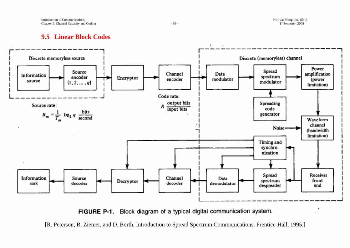
9.5 Linear Block Codes
[R. Peterson, R. Ziemer, and D. Borth, Introduction to Spread Spectrum Communications. Prentice-Hall, 1995.]

Introduction to Communications Prof. Jae Hong Lee, SNU Chapter 9. Channel Capacity and Coding - 57 - 1st Semester, 2008
An ( , )n k (binary) block code† is completely defined by 2kM = binary sequences of length n called
codewords.
For the time being we consider only binary codes.
A code C consists of M codewords ic for 1 2ki≤ ≤ , that is,
1 2{ , , , }MC = c c c
where each ic is a sequence if length n with components equal to 0 or 1.
Definition 9.5.1.
A block code is linear if any linear combination of two codewords is also a codeword.
In the binary case this requires that if ic and jc are codewords then i j⊕c c is also a codeword, where ⊕
stands for component-wise modulo- 2 addition.
A linear block code is a k -dimensional subspace of an n -dimensional space.
It is also obvious that the all zero sequence 0 is a codeword of any linear block code since it can be written † From now on we will deal with binary codes unless otherwise specified.

Introduction to Communications Prof. Jae Hong Lee, SNU Chapter 9. Channel Capacity and Coding - 58 - 1st Semester, 2008
as i i⊕c c for any codeword ic .
Note that linearity of a code only depends on the codewords and not on the way that the information
sequences (messages) are mapped to the codewords.
From now on we assume the linear codes we study satisfies a special property that if the information
sequence 1x (of length k ) is mapped into the codeword 1c (of length n ) and the information sequence 2x
is mapped into 2c , then 1 2⊕x x is mapped into 1 2⊕c c .
Ex.9.5.1
A (5, 2) code is defined by
{00000,10100, 01111,11011}C = .
Verify that this code is linear.
Solution
a) If the mapping between the information sequences and codewords is given by

Introduction to Communications Prof. Jae Hong Lee, SNU Chapter 9. Channel Capacity and Coding - 59 - 1st Semester, 2008
00 0000001 0111110 1010011 11011
→→→→
then, the special property mentioned above is satisfied as well.
b) If the mapping is given by 00 1010001 0111110 0000011 11011,
→→→→
then, the special property is not satisfied.
However, in both cases the code is linear.
Definition 9.5.3
The Hamming weight, or simply the weight, ( )iw c of a codeword ic is the number of nonzero components
of the codeword.
Definition 9.5.2

Introduction to Communications Prof. Jae Hong Lee, SNU Chapter 9. Channel Capacity and Coding - 60 - 1st Semester, 2008
The Hamming distance ( , )i jd c c between two codewords ic and jc is the number of components at
which the two codewords differ,† that is,
( , ) ( )i j i jd w= −c c c c
Definition 9.5.4
The minimum distance of a code mind is the minimum Hamming distance between any two different
codewords in the code, that is,
min ,min ( , )
i ji j
i j
d d≠
=c c
c c . (9.5.1)
Definition 9.5.5
The minimum weight of a code minw is the minimum of the weights of the codewords except the all-zero
codeword, that is,
min min ( )i
iw w≠
=c 0
c . (9.5.2)
Theorem 9.5.1
In any linear code, min mind w= .
† From now on Hamming distance is denoted by d and Euclidean distance is denoted by Ed .

Introduction to Communications Prof. Jae Hong Lee, SNU Chapter 9. Channel Capacity and Coding - 61 - 1st Semester, 2008
Proof
If c is a codeword, then ( ) ( , )iw d=c c 0 .
min ,min ( , )
i ji j
i j
d d≠
=c c
c c
,
min ( )i j
i j
i j
w≠
= −c c
c c
min ( )
l
l
lw≠
=c
c 0
c
minw= .
This implies that, in a linear code, corresponding to any weight of a codeword, there exists a Hamming
distance between two codewords; and corresponding to any Hamming distance, there exists a weight of a
codeword.
Generator and Parity Check Matrices In an ( , )n k (binary) linear block code, let the codeword corresponding to the information sequences
1 (1000 0)=e , 2 (0100 0)=e , 3 (0010 0)=e , , (0000 1)k =e of length k be denoted by
1 2 3, , , , kg g g g of length n , respectively, where each of the ig sequences is a binary sequences of length

Introduction to Communications Prof. Jae Hong Lee, SNU Chapter 9. Channel Capacity and Coding - 62 - 1st Semester, 2008
n .
Now, any information sequence 1 2 3( , , , , )kx x x x=x can be written as
1
n
i ii
x=
=∑x e (9.5.3)
and the corresponding codeword is given by
1
n
i ii
x=
=∑c g . (9.5.4)
If we define the generator matrix for this code as
1
2
k
⎡ ⎤⎢ ⎥⎢ ⎥⎢ ⎥⎢ ⎥⎣ ⎦
gg
G
g
11 12 1
21 22 2
1 2
n
n
k k kn
g g gg g g
g g g
⎡ ⎤⎢ ⎥⎢ ⎥=⎢ ⎥⎢ ⎥⎣ ⎦
, (9.5.5)
then, we can write
=c xG . (9.5.6)

Introduction to Communications Prof. Jae Hong Lee, SNU Chapter 9. Channel Capacity and Coding - 63 - 1st Semester, 2008
This shows that any linear combination of the rows of the generator matrix is a codeword.
The generator matrix for any linear block code is a k n× matrix of rank k (because the dimension of the
subspace is k , by definition).
The generator matrix of a code completely describes the code, that is, when the generator matrix is given,
the structure of an encoder is quite simple.
Ex. 9.5.2
Find the generator matrix for the first code given in Example 9.5.1.
Solution
We have to find the codewords corresponding to information sequences 10 and 01 which are orthogoanl.
These are 10100 and 01111, respectively.
Therefore, we have

Introduction to Communications Prof. Jae Hong Lee, SNU Chapter 9. Channel Capacity and Coding - 64 - 1st Semester, 2008
1010001111⎡ ⎤
= ⎢ ⎥⎣ ⎦
G (9.5.7)
It is seen that for the information sequence 1 2( , )x x , the codeword is given by
1 2 3 4 5 1 2( , , , , ) ( , )c c c c c x x= G (9.5.8)
or
1 1c x=
2 2c x=
3 1 2c x x= ⊕
4 2c x=
5 2c x=
The codeword corresponding to each information sequence starts with a replica of the information sequence
itself followed by some extra bits.
Such a code is called a systematic code and the extra bits following the information sequence in the
codeword are called the parity check bits or redundant bits (or redundancy).

Introduction to Communications Prof. Jae Hong Lee, SNU Chapter 9. Channel Capacity and Coding - 65 - 1st Semester, 2008
A code which is not systematic is called a non-systematic code.
A necessary and sufficient condition for a code to be systematic is that the generator matrix be in the form
[ | ]k=G I P (9.5.9)
where kI denotes a k k× identity matrix and P is a ( )k n k× − binary matrix.
In a systematic code, we have
1
, 1 ,
, 1 ,
ik
ij i j
j
x i kc
p x k i n=
≤ ≤⎧⎪= ⎨ + ≤ ≤⎪⎩∑
(9.5.10)
where summations are modulo- 2 .
By definition, a linear block code C is a k -dimensional linear subspace of the n -dimensional space.
If we take all sequences of length n that are orthogonal to all vectors in this k -dimensional linear
subspace, the result will be an ( )n k− -dimensional linear subspace called the orthogonal complement of the
k -dimensional subspace.

Introduction to Communications Prof. Jae Hong Lee, SNU Chapter 9. Channel Capacity and Coding - 66 - 1st Semester, 2008
This ( )n k− -dimensional linear subspace defines an ( , )n n k− linear code which is known as the dual of
the original ( , )n k code C .
The dual code is denoted by C⊥ .
The codewords of the original code C and the dual code C⊥ are orthogonal to each other.
In particular, if we denote the generator matrix of the dual code by H , which is an ( )n k n− × matrix, then
any codeword of the original code is orthogonal to all rows of H , that is, T =c H 0 for all C∈c . (9.5.11)
The matrix H , which is the generator matrix of the dual code C⊥ , is called the parity check matrix of the
original code C .
Since all rows of the generator matrix are codewords, we have T =GH 0 . (9.5.12)
In the special case of a systematic code where

Introduction to Communications Prof. Jae Hong Lee, SNU Chapter 9. Channel Capacity and Coding - 67 - 1st Semester, 2008
[ | ]k=G I P , (9.5.13)
the parity check matrix is given in the form of
[ | ]Tk= −H P I . (9.5.14)
Note that T T− =P P in the case of binary code.
Ex. 9.5.3
Find the parity check matrix for the code given in Example 9.5.1.
Solution
Here
1010001111⎡ ⎤
= ⎢ ⎥⎣ ⎦
G
1001⎡ ⎤
= ⎢ ⎥⎣ ⎦
I
100111⎡ ⎤
= ⎢ ⎥⎣ ⎦
P .

Introduction to Communications Prof. Jae Hong Lee, SNU Chapter 9. Channel Capacity and Coding - 68 - 1st Semester, 2008
Since T T− =P P in the case of binary code, we have
110101
t
⎡ ⎤⎢ ⎥= ⎢ ⎥⎢ ⎥⎣ ⎦
P
and, hence,
11 10001 01001 001
⎡ ⎤⎢ ⎥= ⎢ ⎥⎢ ⎥⎣ ⎦
H .
Hamming Codes Hamming codes are a class of ( , )n k linear block codes with 2 1,mn = − 2 1,mk m= − − and min 3d = , for
some integer 2m ≥ .
These codes are capable of correcting all single errors.
The parity check matrix for a Hamming code consists of all binary sequences of length m except the all-
zero sequence.

Introduction to Communications Prof. Jae Hong Lee, SNU Chapter 9. Channel Capacity and Coding - 69 - 1st Semester, 2008
The rate of a Hamming code is given by
2 12 1
m
c m
mR − −=
− (9.5.15)
which becomes close to 1 as m takes large values.
Hamming codes are high-rate codes with relatively small minimum distance min( 3)d = .
Ex. 9.5.4
Find the parity check matrix and the generator matrix of a (7, 4) Hamming code in the systematic form.
Solution
Since 2 1 7mn = − = , 3m = .
Hence, the parity check matrix H consists of all binary sequences of length 3 except the all-zero
sequence.

Introduction to Communications Prof. Jae Hong Lee, SNU Chapter 9. Channel Capacity and Coding - 70 - 1st Semester, 2008
The parity check matrix in the systematic form is given by
1 0 1 1 1 0 01 1 0 1 0 1 00 1 1 1 0 0 1
⎡ ⎤⎢ ⎥= ⎢ ⎥⎢ ⎥⎣ ⎦
H
[ | ]T
k= −P I
and the generator matrix is obtained as
[ | ]k=G I P
1 0 0 0 1 1 00 1 0 0 0 1 10 0 1 0 1 0 10 0 0 1 1 1 1
⎡ ⎤⎢ ⎥⎢ ⎥=⎢ ⎥⎢ ⎥⎣ ⎦
G .
9.5.1 Decoding and Performance of Linear Block Codes
The purpose of using channel coding in communication systems is to reduce the error probability at a given
transmitted power by increasing the Euclidean distance between the transmitted signals.
Hence, codes are compared is based on the minimum distance of the code, which is equal to the minimum

Introduction to Communications Prof. Jae Hong Lee, SNU Chapter 9. Channel Capacity and Coding - 71 - 1st Semester, 2008
weight for linear codes.
For a given n and k , a code with a larger minimum distance, mind (or minw ), usually has better
performance than a code with a smaller minimum distance.
Soft-Decision Decoding
In the optimum signal-detection scheme on an additive white Gaussian noise channel, detection is made such
that the Euclidean distance between the received signal and the transmitted signal is minimized.
In using coded waveforms the concept is the same.
Assuming that binary PSK is adopted for transmission of the coded message, a codeword
1 2( , , , )i i i i nc c c=c is mapped into the sequence ( )1
( ) ( 1)n
i ikk
s t t k Tψ=
= − −∑ , where
( ), 1,( )
( ), 0,ik
ikik
t ct
t cψ
ψψ
=⎧= ⎨− =⎩
(9.5.16)
and the waveform ( )tψ has duration T and energy ε , and is equal to zero outside the interval [0, ]T .

Introduction to Communications Prof. Jae Hong Lee, SNU Chapter 9. Channel Capacity and Coding - 72 - 1st Semester, 2008
The Euclidean distance between any two signal waveforms is given by 2 2
1:
( ) ( )
i l j l
Eij i l j l
l nl c c
d c c≤ ≤≠
= −∑
2
1:
(2 )
i l j l
l nl c c
ε≤ ≤≠
= ∑
H4 i jd ε= . (9.5.17)
For orthogonal signaling, where 1( )tψ and 2 ( )tψ are orthogonal, the Euclidean distance between any two
signal waveforms is given by
( )221 201
:
( ) ( ) ( )
i l j l
TEij
l nl c c
d t t dtψ ψ≤ ≤≠
= −∑ ∫
2
1:
( 2 )
i l j l
l nl c c
ε≤ ≤≠
= ∑
2 Hi jd ε= . (9.5.18)

Introduction to Communications Prof. Jae Hong Lee, SNU Chapter 9. Channel Capacity and Coding - 73 - 1st Semester, 2008
Using the relation
02
E
edP Q
N
⎛ ⎞= ⎜ ⎟⎜ ⎟
⎝ ⎠, (9.5.19)
we obtain
0
0
, for orthogonal signaling,
( received | sent)2
, for antipodal signaling.
i j
i j
dQ
NP j i
dQ
N
ε
ε
⎧ ⎛ ⎞⎪ ⎜ ⎟⎜ ⎟⎪⎪ ⎝ ⎠= ⎨
⎛ ⎞⎪⎜ ⎟⎪ ⎜ ⎟⎪ ⎝ ⎠⎩
(9.5.20)
Since ( )Q x is a decreasing function of x and minijd d≥ , we have
min
0
min
0
, for orthogonal signaling,
( received | sent)2 , for antipodal signaling.
dQN
P j idQ
N
ε
ε
⎧ ⎛ ⎞⎪ ⎜ ⎟⎜ ⎟⎪ ⎝ ⎠= ⎨
⎛ ⎞⎪⎜ ⎟⎪ ⎜ ⎟⎝ ⎠⎩
(9.5.21)
Using the union bound (see Chapter 7), we obtain

Introduction to Communications Prof. Jae Hong Lee, SNU Chapter 9. Channel Capacity and Coding - 74 - 1st Semester, 2008
min
0
min
0
( 1) , for orthogonal signaling,
(error | sent)2( 1) , for antipodal signaling.
dM QN
P idM QN
ε
ε
⎧ ⎛ ⎞−⎪ ⎜ ⎟⎜ ⎟⎪ ⎝ ⎠= ⎨
⎛ ⎞⎪ − ⎜ ⎟⎪ ⎜ ⎟⎝ ⎠⎩
(9.5.22)
Assuming equiprobable messages, we have
min
0
min
0
( 1) , for orthogonal signaling,
2( 1) , for antipodal signaling.e
dM QN
PdM QN
ε
ε
⎧ ⎛ ⎞−⎪ ⎜ ⎟⎜ ⎟⎪ ⎝ ⎠≤ ⎨
⎛ ⎞⎪ − ⎜ ⎟⎪ ⎜ ⎟⎝ ⎠⎩
(9.5.23)
In optimal demodulation, the received signal ( )r t is passed through a bank of matched filters to obtain the
received vector r , and then the closet point in the constellation to r is found in the Euclidean distance sense.
The type of decoding which involves finding the minimum Euclidean distance is called soft-decision
decoding, and requires real number computation.

Introduction to Communications Prof. Jae Hong Lee, SNU Chapter 9. Channel Capacity and Coding - 75 - 1st Semester, 2008
Ex. 9.5.5
Compare the performances of an uncoded data transmission system with a coded transmission using the (7, 4)
Hamming code given in Example 9.5.4.
Assume that a binary source has rate 410R = bits/sec and the modulation scheme is binary PSK.
Also assume that the channel is an additive white Gaussian noise channel, the received power is 1 Wμ , and
the noise power-spectral density is 110 102
N −= .
Solution
1. If no coding is employed, we have
0
2 bbP Q
Nε⎛ ⎞
= ⎜ ⎟⎜ ⎟⎝ ⎠
0
2PQRN
⎛ ⎞= ⎜ ⎟⎜ ⎟
⎝ ⎠. (9.5.24)
As 6
4 110
2 1010 10
PRN
−
−=×
10= , we have

Introduction to Communications Prof. Jae Hong Lee, SNU Chapter 9. Channel Capacity and Coding - 76 - 1st Semester, 2008
( 10)bP Q=
(3.16)Q=
47.86 10−≈ × . (9.5.25)
The error probability for a four-bit sequence is given by 4
error in 4 bits 1 (1 )bP P= − −
33.1 10−≈ × . (9.5.26)
2. If coding is employed, we have min 3d = , and
0 0
bcR
N Nε ε
=
0c
PRRN
=
4 57
= ×
207
= .
The message error probability is given by
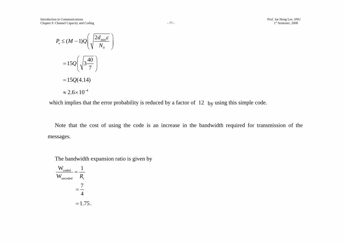
Introduction to Communications Prof. Jae Hong Lee, SNU Chapter 9. Channel Capacity and Coding - 77 - 1st Semester, 2008
min
0
2( 1)edP M QN
ε⎛ ⎞≤ − ⎜ ⎟⎜ ⎟
⎝ ⎠
4015 37
Q⎛ ⎞
= ⎜ ⎟⎝ ⎠
15 (4.14)Q=
42.6 10−≈ ×
which implies that the error probability is reduced by a factor of 12 by using this simple code.
Note that the cost of using the code is an increase in the bandwidth required for transmission of the
messages.
The bandwidth expansion ratio is given by
coded
uncoded
W 1W cR
=
74
=
1.75= .

Introduction to Communications Prof. Jae Hong Lee, SNU Chapter 9. Channel Capacity and Coding - 78 - 1st Semester, 2008
Hard-Decision Decoding
A simpler decoding scheme is to make hard binary decisions on the components of the received vector r , and
then to find the codeword which is closest to it in the sense of Hamming distance.
Ex.9.5.6
A (3,1) code consists of the two codewords 000 and 111.
The codewords are transmitted using binary PSK modulation with 1ε = .
Suppose that the received vector (that is, the sampled outputs of the matched filters) is (0.5, 0.5, 3)= −r .
In soft decision decoding, we compare the Euclidean distance between r and the two signal points (1,1,1)
which corresponds to 111 and ( 1, 1, 1)− − − which corresponds to 000 and choose the signal point which
gives smaller distance.
We have
( )2E 2 2 2( , (1,1,1) 0.5 0.5 4 16.5d = + + =r and

Introduction to Communications Prof. Jae Hong Lee, SNU Chapter 9. Channel Capacity and Coding - 79 - 1st Semester, 2008
( )2E 2 2 2( ,( 1, 1, 1) 1.5 1.5 ( 2) 8.5d − − − = + + − =r
Hence, In soft-decision decoding the decoder would decode r as ( 1, 1, 1)− − − or, equivalently, (0, 0, 0) .
However, if hard-decision decoding is employed, r is first component-wise detected as 1 or 0 .
The resulting vector y is therefore (1,1, 0)=y .
Hence, in hard-decision decoding the decoder compare y with the (1,1,1) and (0, 0, 0) and find the
closer one in the Hamming distance sense, of which result is (1,1,1) .
Notice that the results of soft-decision decoding and hard-decision decoding can be different.
Soft-decision decoding is the optimal detection method and achieves a lower probability of error than hard-
decision decoding
There are three basic steps involved in hard-decision decoding.

Introduction to Communications Prof. Jae Hong Lee, SNU Chapter 9. Channel Capacity and Coding - 80 - 1st Semester, 2008
First, we perform demodulation by passing the received ( )r t through the matched filters and sampling the
output to obtain the r vector.
Second, we compare the components of r with the thresholds and quantize each component to one of the
two levels to obtain y vector.
Third, we perform decoding by finding the codeword that is closest to y in the sense of Hamming distance.
In this section, we present a systematic approach to perform hard-decision decoding.
First, we introduce a standard array.
Let the codewords of the code be denoted by 1 2, , , Mc c c , where each of them is of length n and
2kM = , and let 1c denote the all-zero codeword.
A standard array is a 2 2n k k− × array whose elements are binary sequences of length n and is generated by
writing all the codewords in a row starting with the all zero codeword.

Introduction to Communications Prof. Jae Hong Lee, SNU Chapter 9. Channel Capacity and Coding - 81 - 1st Semester, 2008
This constitutes the first row of the standard array.
To write the second row, we look among all the binary sequences of length n that are not in the first row
of the array.
Choose one of these sequences that has the minimum weight and denote it by 1e .
Write it under† 1c and write 1 i⊕e c under ic for 2 i M≤ ≤ .
The third row of the array is written similarly to the second row as follows.
From the binary n -tuples that have not been used in the first two rows, we choose one with minimum
weight and call it 2e .
Then, the elements of the third row become 2i ⊕c e , 2 i M≤ ≤ .
† Note that 1 1 1⊕ =c e e , since 1 (0, 0, , 0)c = .

Introduction to Communications Prof. Jae Hong Lee, SNU Chapter 9. Channel Capacity and Coding - 82 - 1st Semester, 2008
This process is continued until no binary n -tuples remains to start a new row.
Figure 9.16 shows the standard array generated as explained above.
Figure 9.16 Standard array.
Each row of the standard array is called a coset and the first element of each coset ( le , in general) is called
the coset leader.

Introduction to Communications Prof. Jae Hong Lee, SNU Chapter 9. Channel Capacity and Coding - 83 - 1st Semester, 2008
Theorem 9.5.2.
All elements of the standard array are distinct.
Proof.
Assume that two elements of the standard array are equal.
This can happen in two ways.
1. The two equal elements belong to the same coset.
In this case we have l i l j⊕ = ⊕c c e c , from which we conclude i j=c c which is impossible.
2. The two equal elements belong to two different cosets.
In this case we have l i k j⊕ = ⊕e c e c , for l m≠ , which means ( ) ( )cl k j i k j i= ⊕ ⊕ = ⊕ ⊕e e c c e c c
where cic is a complement of ic modulo 2
By linearity of the code i j⊕c c is also a codeword which is denoted by mc .
Therefore, l k m= ⊕e e c and, hence, le and ke belong to the same coset, which is impossible since by

Introduction to Communications Prof. Jae Hong Lee, SNU Chapter 9. Channel Capacity and Coding - 84 - 1st Semester, 2008
assumption k l≠ .
From Theorem 9.5.2, we conclude that the standard array contains exactly
# of sequences of length 2 2# of codewords 2
nn k
k
n −= = rows.
Theorem 9.5.3.
If 1y and 2y are elements of the same coset, we have 1 2T T=y H y H .
Proof.
Since 1y and 2y are in the same coset, 1 l i= ⊕y e c and 2 l j= ⊕y e c , where i j≠c c , therefore
1 ( )T Tl i= ⊕y H e c H
Tl= +e H 0
( ) Tl j= ⊕e c H
2T= y H .
From Theorem 9.5.3, we conclude that each coset of the standard array is uniquely identified by the product T
le H .

Introduction to Communications Prof. Jae Hong Lee, SNU Chapter 9. Channel Capacity and Coding - 85 - 1st Semester, 2008
For any binary sequence y of length n , we define the syndrome s as T=s yH . (9.5.27)
If l i= ⊕y e c , that is, y belongs to the ( 1)l + st coset, then obviously Tl=s e H .
The syndrome is a binary sequence of length n k− and there exists a unique syndrome corresponding to
each coset.
Obviously, the syndrome corresponding to the first coset, which consists of the codewords, is T=s 0H = 0 .
Ex.9.5.7
Find the standard array for the (5, 2) code with codewords 00000, 10100, 01111, 11011.
Also find the syndromes corresponding to each coset.
Solution
The generator polynomial of the code is given by

Introduction to Communications Prof. Jae Hong Lee, SNU Chapter 9. Channel Capacity and Coding - 86 - 1st Semester, 2008
1 0 1 0 00 1 1 1 1⎡ ⎤
= ⎢ ⎥⎣ ⎦
G
and the parity check matrix corresponding to G is given by
1 1 1 0 00 1 0 1 00 1 0 0 1
⎡ ⎤⎢ ⎥= ⎢ ⎥⎢ ⎥⎣ ⎦
H .
Using the construction procedure described before, the standard array is obtained as
00000 01111 10100 11011 syndrome 00010000 11111 00100 01011 syndrome 10001000 00111 11100 10011 syndrome 11100010 01101 10110 11001 syndrome 01000001 01110 10101 11010 syndrome 00111000 10111 01100 00011 syndrome 01110010 111
======
01 00110 01001 syndrome 11010001 11110 00101 01010 syndrome 101
==
Assume that that the received vector r is compared component-wise with a threshold for hard decision
and the resulting binary vector is y .
Then, find the codeword which is at the shortest Hamming distance from y .

Introduction to Communications Prof. Jae Hong Lee, SNU Chapter 9. Channel Capacity and Coding - 87 - 1st Semester, 2008
First, we find the coset in which y is located .
To do this, calculate the syndrome of y by T=s yH and refer to the standard array to find the coset
corresponding to s .
Suppose that the coset leader corresponding to this coset is le .
Then, l i= ⊕y e c for some i , because y belongs to this coset.
Hence, the Hamming distance of y from any codeword jc is given by
( , ) ( )j jd w= ⊕y c y c
( )l i jw= ⊕ ⊕e c c . (9.5.28)
Because the code C is linear, i j⊕c c is also a codeword, that is, i j k⊕ =c c c for some integer k ,
1 k M≤ ≤ .
This implies that

Introduction to Communications Prof. Jae Hong Lee, SNU Chapter 9. Channel Capacity and Coding - 88 - 1st Semester, 2008
( , ) ( )j k ld w= ⊕y c c e (9.5.29)
where k l⊕c e belongs to the same coset which y belongs to.
Therefore, to minimize ( , )jd y c , we have to find the minimum weight element in the coset to which y
belongs.
By the construction procedure of the standard array, this element is the coset leader, that is, we choose
k =c 0 and, therefore, j i=c c .
This implies that y is decoded into i=c c by finding
l= ⊕c y e
i= c . (9.5.30)
This procedure for hard-decision decoding can be summarized as follows.
1. Find r , the vector representation of the received signal.
2. Compare each component of r to the optimal threshold (usually 0 ) and make a binary decision on it to

Introduction to Communications Prof. Jae Hong Lee, SNU Chapter 9. Channel Capacity and Coding - 89 - 1st Semester, 2008
obtain the binary vector y .
3. Find T=s yH the syndrome of y .
4. Find the coset corresponding to s by using the standard array.
5. Find the coset leader e and decoded y as = ⊕c y e .
Because in this decoding scheme the difference between the vector y and the decoded vector c is e , the
binary n -tuple e is frequently referred to as the error pattern.
This means that the coset leaders constitute the set of all correctable error patterns.
In hard-decision decoding the error probability for each bit for antipodal signaling is given by
0
2 bbP Q
Nε⎛ ⎞
= ⎜ ⎟⎜ ⎟⎝ ⎠
(9.5.31)
and that for orthogonal signaling is given by

Introduction to Communications Prof. Jae Hong Lee, SNU Chapter 9. Channel Capacity and Coding - 90 - 1st Semester, 2008
0
bbP Q
Nε⎛ ⎞
= ⎜ ⎟⎜ ⎟⎝ ⎠
. (9.5.32)
The channel between the input codeword c and the output of the hard limiter y is a binary-input binary-
output channel that can be modeled by a binary-symmetric channel with crossover probability bP .
Because the code is linear, the distance between any two codeword ic and jc is the distance between the
all-zero codeword 0 and i j k⊕ =c c c .
Assume that the all-zero codeword 0 is transmitted without loss of generality.
By the union bound, the error probability cannot exceed ( 1)M − times the probability of decoding into the
codeword that is closet to 0 in the sense of Hamming distance.
For this codeword, denoted by c , which is at distance mind from 0 , we have

Introduction to Communications Prof. Jae Hong Lee, SNU Chapter 9. Channel Capacity and Coding - 91 - 1st Semester, 2008
minmin
min
min minminmin
min
minmin
12
minmin 2 2
minmin1
2
(1 ) , odd,
(decode to | sent)1(1 ) (1 ) , even,2
2
dd ii
b bdi
d ddd ii
b b b bdi
dP P d
i
P ddP P P P ddi
−
+=
−
= +
⎧ ⎛ ⎞−⎪ ⎜ ⎟
⎝ ⎠⎪⎪≤ ⎨ ⎛ ⎞⎪ ⎛ ⎞ ⎜ ⎟− + −⎪ ⎜ ⎟ ⎜ ⎟⎝ ⎠⎪ ⎝ ⎠⎩
∑
∑c 0
or, in general, min
min
min
min
12
(decode to | sent) (1 )d
d iib b
di
dP P P
i−
+⎢ ⎥=⎢ ⎥⎣ ⎦
⎛ ⎞≤ −⎜ ⎟
⎝ ⎠∑c 0 . (9.5.33)
Therefore,
( 1) (decode to | sent)eP M P≤ − c 0
minmin
min
min
12
( 1) (1 )d
d iib b
di
dM P P
i−
+⎢ ⎥=⎢ ⎥⎣ ⎦
⎛ ⎞≤ − −⎜ ⎟
⎝ ⎠∑ (9.5.34)
which is an upper bound on the error probability of a linear block code using hard-decision decoding.
Both in soft-decision and hard-decision decoding, mind plays a major role in bounding the error probability.
For a given ( , )n k , it is desirable to have codes with large mind .

Introduction to Communications Prof. Jae Hong Lee, SNU Chapter 9. Channel Capacity and Coding - 92 - 1st Semester, 2008
It can be shown that soft-decision decoding has roughly 2 dB better performance than hard-decision
decoding for an additive white Gaussian noise channel.
It can also be shown that if an 8 -level quantizer (three bits/component) is employed instead of to a 2 -level
quantizer for each component of r , performance difference with soft decision (with infinite precision)
reduces to 0.1 dB.
This multilevel quantization scheme, which is a compromise between soft decision (having infinite
precision) and hard decision, is also referred to as soft decision in the literature.
Ex.9.5.8
If hard-decision decoding is employed in Example 9.5.5, how will the results change?
Solution
Here 40 (2.39) 0.00847bP Q Q
⎛ ⎞= = =⎜ ⎟
⎝ ⎠ and
min 3d = .

Introduction to Communications Prof. Jae Hong Lee, SNU Chapter 9. Channel Capacity and Coding - 93 - 1st Semester, 2008
Therefore,
2 5 3 4 77 7(1 ) (1 )
2 3e b b b b bP P P P P P⎛ ⎞ ⎛ ⎞
≤ − + − + +⎜ ⎟ ⎜ ⎟⎝ ⎠ ⎝ ⎠
221 bP≈ 31.5 10−≈ × .
In this case, coding has decreased the error probability by a factor of 2 , compared to 12 in the soft-
decision case.
Error Detection versus Error Correcting Let C be a linear block code with minimum distance mind .
Then, if c is transmitted and hard-decision decoding is employed, any codeword will be decoded correctly
if the received y is closer to c than any other codeword as shown in Figure 9.17.

Introduction to Communications Prof. Jae Hong Lee, SNU Chapter 9. Channel Capacity and Coding - 94 - 1st Semester, 2008

Introduction to Communications Prof. Jae Hong Lee, SNU Chapter 9. Channel Capacity and Coding - 95 - 1st Semester, 2008
As shown in Figure 9.17, around each codeword there is a “Hamming sphere” of radius ce where ce is
the number of correctable errors.
As long as these spheres are disjoint, the code is capable of correcting ce errors.
The condition for nonoverlapping spheres is expressed as
min min
min min
2 1 , odd,2 2 , even,
c
c
e d de d d+ =⎧
⎨ + =⎩
or
minmin
minmin
1, odd,2
2 , even,2
c
d de
d d
−⎧⎪⎪= ⎨ −⎪⎪⎩
(9.5.35)
which can be summarized as
min 12c
de −⎢ ⎥= ⎢ ⎥⎣ ⎦. (9.5.36)

Introduction to Communications Prof. Jae Hong Lee, SNU Chapter 9. Channel Capacity and Coding - 96 - 1st Semester, 2008
In a communication system where a feedback link is available from the receiver to the transmitter, it might
be desirable to detect if an error has occurred and, if so, to ask the transmitter via the feedback channel to
retransmit the message.
The error-detection capability of a code in the absence of error correction is given by min 1de d= − , because
if min 1d − or fewer errors occur, the transmitted codeword will be converted to a word sequence which is not
a codeword and, therefore, an error is detected.
If both error correction and error detection are desirable, then there is a trade-off between them as shown
Figure 9.18.

Introduction to Communications Prof. Jae Hong Lee, SNU Chapter 9. Channel Capacity and Coding - 97 - 1st Semester, 2008
Figure 9.18 Relation between ce , de and mind .
In Figure 9.18, we see that
min 1c de e d+ = − (9.5.37)
with the extra condition c de e≤ .

Introduction to Communications Prof. Jae Hong Lee, SNU Chapter 9. Channel Capacity and Coding - 98 - 1st Semester, 2008
9.5.2 Burst-Error-Correcting-Codes
Most of the linear block codes are designed for correcting random errors, that is, errors that occur
independently from the location of other channel errors.
Channel models including the additive white Gaussian noise channel can be modeled as channels with
random errors.
However, the assumption of independently generated errors is not a valid in some other physical channels
such as a fading channel.
In such a channel, if the channel is in deep fade, a large number of errors occur in sequence, that is, the
errors are bursty.
In this channel, the probability of error at a certain location or time depends on whether its adjacent bits are
received correctly or not.
Another example of a channel with burst error is a compact disc.

Introduction to Communications Prof. Jae Hong Lee, SNU Chapter 9. Channel Capacity and Coding - 99 - 1st Semester, 2008
Any physical damage to a compact disc, such as a scratch, damages a sequence of bits and, therefore, the
errors tend to occur in bursts.
Any random error-correcting code can be used to correct burst errors as long as the number of errors is less
than half of the minimum distance of the code.
But there are more efficient coding schemes to correct burst errors such as Fire codes and Burton codes.
An effective method for correction of error bursts is to interleave the coded data such that the location of
errors looks random and is distributed over many codewords rather than a few codewords.
In this way, the number of errors that occur in each block becomes small and can be corrected by using a
random error correcting code.
At the receiver, a deinterleaver is employed to reverse the effect of the interleaver.
A block diagram of a coding system employing interleaving/deinterleaving is shown in Figure 9.19.

Introduction to Communications Prof. Jae Hong Lee, SNU Chapter 9. Channel Capacity and Coding - 100 - 1st Semester, 2008
Figure 9.19 Block diagram of a system that employs interleaving/deinterleaving for burst-error-correction.
An interleaver of depth m reads m codewords of length n each and arranges them in a block with m
rows and n columns.
Then, this block is read by column and the output is sent to the digital modulator.
At the receiver, the output of the detector is supplied to the deinterleaver, which generates the same m n×
block structure and then reads by row and sends the output to the channel decoder as shown in Figure 9.20.

Introduction to Communications Prof. Jae Hong Lee, SNU Chapter 9. Channel Capacity and Coding - 101 - 1st Semester, 2008

Introduction to Communications Prof. Jae Hong Lee, SNU Chapter 9. Channel Capacity and Coding - 102 - 1st Semester, 2008
Assume that 8m = and the code in use is a (15,11) Hamming code capable of correcting one
error/codeword.
Then, the block generated by the interleaver is a 8 15× block containing 120 binary symbols.
Any burst of errors of length 8 or less will result in at most one error/codeword and, therefore, can be
corrected by the decoding of (15,11) Hamming code.
If interleaving/deinterleaving was not employed, an error burst of length 8 could possibly result in
erroneous detection in 2 codewords (up to 22 information bits).

Introduction to Communications Prof. Jae Hong Lee, SNU Chapter 9. Channel Capacity and Coding - 103 - 1st Semester, 2008
9.6 Cyclic Codes
Cyclic codes are a subset of linear block codes for which easily implementable encoders and decoders exists.
Definition 9.6.1.
A cyclic code is a linear block code with the extra condition that if c is a codeword, a cyclic shift† of it is
also a codeword.
Ex.9.6.1
The code {000,110,101, 011} is a cyclic code because it is easily verified to be linear and a cyclic shift of any
codeword is also a codeword.
The code {000, 010,101,111} is not cyclic because, although it is linear, a cyclic shift of 101 is not a
codeword.
† A cyclic shift of the codeword 1 2 1( , , , , )n nc c c c−=c is defined to be (1)2 3 1 1( , , , , , )n nc c c c c−=c .

Introduction to Communications Prof. Jae Hong Lee, SNU Chapter 9. Channel Capacity and Coding - 104 - 1st Semester, 2008
9.6.1 Structure of Cyclic Codes
To study the properties of cyclic codes, it is easier to represent each codeword as a polynomial, called the
codeword polynomial.
The codeword polynomial corresponding to 1 2 1( , , , , )n nc c c c−=c is simply defined to be
1 1 21 2 1
1( )
nn n n
i n ni
c p c p c p c p c p c− − −−
=
= = + + + +∑ . (9.6.1)
The codeword polynomial of (1)2 3 2 1 1( , , , , , , )n n nc c c c c c− −=c , the cyclic shift of c , is
(1) 1 2 22 3 1 1( ) n n
n nc p c p c p c p c p c− −−= + + + + + (9.6.2)
which can be written as (1)
1( ) ( ) ( 1)nc p pc p c p= + + . (9.6.3)
Nothing that in the binary field addition and subtraction are equivalent, this reduces to (1)
1( ) ( ) ( 1)npc p c p c p= + + (9.6.4)
or (1) ( ) ( ) (mod ( 1))nc p pc p p= + . (9.6.5)

Introduction to Communications Prof. Jae Hong Lee, SNU Chapter 9. Channel Capacity and Coding - 105 - 1st Semester, 2008
If we shift (1)c once more the result will also be a codeword and its codeword polynomial will be (2) (1)( ) ( ) (mod ( 1))nc p pc p p= + (9.6.6)
2 ( ) (mod ( 1))np c p p= + (9.6.7)
where
( ) ( ) (mod ( ))a p b p d p=
means that ( )a p and ( )b p have the same remainder when divided by ( )d p .
In general, for i shifts we have the codeword polynomial ( ) ( ) ( ) (mod( 1))i i nc p p c p p= + . (9.6.8)
For i n= , we have ( ) ( ) ( ) (mod ( 1))n n nc p p c p p= + (9.6.9)
( 1) ( ) ( ) (mod( 1))n np c p c p p= + + + (9.6.10)
( )c p= (9.6.11)
which is obvious because shifting any codeword n times leaves it unchanged.

Introduction to Communications Prof. Jae Hong Lee, SNU Chapter 9. Channel Capacity and Coding - 106 - 1st Semester, 2008
Theorem 9.6.1.
In any ( , )n k cyclic code all codeword polynomials are multiples of a polynomial of degree n k− of the
form 1 2
2 3( ) 1n k n k n kn kg p p g p g p g p− − − − −−= + + + + +
called the generator polynomial, where ( )g p divides 1np + .
Furthermore, for any information sequence 1 2 1( , , , , )k kx x x x−=x , we have the information sequence
polynomial ( )X p defined by 1 2
1 2 1( ) k kk kX p x p x p x p x− −−= + + + +
and the codeword polynomial corresponding to x is given by ( ) ( ) ( )c p X p g p= .
Any codeword polynomial is the product of the generator polynomial and the information polynomial.
That is, 1 2 1( , , , , )n nc c c c−=c is the discrete convolution of the two sequences 1 2( , , , )kx x x=x and
2(1, , , ,1)n kg g −=g .

Introduction to Communications Prof. Jae Hong Lee, SNU Chapter 9. Channel Capacity and Coding - 107 - 1st Semester, 2008
9.7 Convolutional Codes
Convolutional codes are different from the block codes by the existence of memory in the encoding scheme.
In block codes, each block (or sequence) of k input bits is mapped into a block of length n of output bits
by a rule defined by the code (for example by G or ( )g p ) and regardless of the previous inputs to the
encoder.
The rate of a block code is given by
ckRn
= . (9.7.1)
In convolutional codes, each block of k bits is again mapped into a block of n bits to be transmitted over
the channel, but these n bits are not only determined by the present k -information bits but also by the
previous information bits.
The block diagram of a convolutional encoder is given in Figure 9.24.

Introduction to Communications Prof. Jae Hong Lee, SNU Chapter 9. Channel Capacity and Coding - 108 - 1st Semester, 2008

Introduction to Communications Prof. Jae Hong Lee, SNU Chapter 9. Channel Capacity and Coding - 109 - 1st Semester, 2008
The convolutional encoder consists of a shift register with kL stages where L is called the constraint
length of the code.
At each instant of time, k -information bits enter the shift register and the contents of the last k stages of
the shift register are dropped.
After the k bits have entered the shift register, n -linear combinations of the contents of the shift register,
as shown in Figure 9.24, are computed to generate the encoded sequence.
The n -encoder outputs not only depend on the most recent k bits that have entered the encoder but also
on the ( 1)L k− contents of the first ( 1)L k− stages of the shift register before the k bits arrived.
Therefore, the shift register is a finite state machine with ( 1)2 L k− states.
Because for each k -input bits, we have n -output bits, the rate of this code is simply given by
ckRn
= . (9.7.2)

Introduction to Communications Prof. Jae Hong Lee, SNU Chapter 9. Channel Capacity and Coding - 110 - 1st Semester, 2008
Ex.9.7.1
An encoder for a convolutional code is shown in Figure 9.25.

Introduction to Communications Prof. Jae Hong Lee, SNU Chapter 9. Channel Capacity and Coding - 111 - 1st Semester, 2008
Figure 9.25 Rate 12
convolutional encoder.
For the encoder in Figure 9.25, 1k = , 2n = , and 3L = .
The rate of the code is 12c
kRn
= = and the number of states is ( 1) (3 1) 12 2 4L k− − ⋅= = .
One way to describe a convolutional code (other than drawing the encoder) is to specify how the two output
bits of the encoder depend on the contents of the shift register by n vectors 1 2, , , ng g g , known as
generator sequences of the convolutional code.
The i th, 1 2kLi≤ ≤ , component of jg , 1 j n≤ ≤ , is 1 if the i th stage of the shift register is connected to
the combiner corresponding to the j th bit in the output and 0 otherwise.
The generator sequences are given by
1 [1 0 1]=g
2 [1 1 1]=g .

Introduction to Communications Prof. Jae Hong Lee, SNU Chapter 9. Channel Capacity and Coding - 112 - 1st Semester, 2008
9.7.1 Basic Properties of Convolutional Codes
Because a convolutional encoder has finite memory, it can be represented by a state-transition diagram.
In the state-transition diagram, each state of the convolutional encoder is represented by a node and
transitions between states are denoted by branches connecting these nodes.
The number of branches emerging from each state is equal to 2k .
Figure 9.26 shows the state transition diagram for the convolutional code in Figure 9.25.

Introduction to Communications Prof. Jae Hong Lee, SNU Chapter 9. Channel Capacity and Coding - 113 - 1st Semester, 2008
Figure 9.26 State transition diagram for the encoder in Figure 9.25.

Introduction to Communications Prof. Jae Hong Lee, SNU Chapter 9. Channel Capacity and Coding - 114 - 1st Semester, 2008
A second method to describe a convolutional code is to specify its trellis diagram.
The trellis diagram is obtained by specifying all states on a vertical axis and repeating this vertical axis
along the time on a horizontal axis.
Then, each transition from a state to another state is denoted by a branches connecting the two states on two
adjacent vertical axes.
As was the case with the state transition diagram, we have 2k branches of the trellis leaving each state and
2k branches merging at each state.
Figure 9.27 shows the trellis diagram for the code described by the encoder in Figure 9.25.

Introduction to Communications Prof. Jae Hong Lee, SNU Chapter 9. Channel Capacity and Coding - 115 - 1st Semester, 2008

Introduction to Communications Prof. Jae Hong Lee, SNU Chapter 9. Channel Capacity and Coding - 116 - 1st Semester, 2008
Encoding
Assume that the encoder, before the first information bit enters it, is loaded with zeros (that is, the encoder is
in the all-zero state).
The information bits enter the encoder k bits at a time and the corresponding n -output bits are
transmitted over the channel.
This procedure is continued until the last group of k bits is loaded into the encoder and the corresponding
n -outputs are transmitted over the channel.
Assume that after the last group of k bits, another group of ( 1)k L − enters encoder so that the
corresponding n outputs are transmitted over the channel. This returns the encoder to the all-zero state to
make it ready for next transmission.
Ex.9.7.2
In the convolutional code shown in Figure 9.25, what is the encoded sequence corresponding to the
information sequence (1101011)=x ?

Introduction to Communications Prof. Jae Hong Lee, SNU Chapter 9. Channel Capacity and Coding - 117 - 1st Semester, 2008
Solution
After transmission of the last information bit, two 0 bits are transmitted which means that the transmitted
sequence is 1 (110101100)=x .
We have the codeword (111010000100101011)=c .
Transfer Function
Any codeword of a convolutional encoder corresponds to a path through the trellis that starts from the all-zero
state and returns to the all-zero state.
To obtain the transfer function of a convolutional code, we split the all-zero state into two states, one
denoting the starting state and one denoting the first return to the all-zero state.
All other states are denoted as in-between states.
Corresponding to each branch connecting two states, a function of the form D N Jα β is defined where α
denotes the number of ones in the output bit sequence for that branch and β is the number of ones in the
corresponding input sequence for that branch.

Introduction to Communications Prof. Jae Hong Lee, SNU Chapter 9. Channel Capacity and Coding - 118 - 1st Semester, 2008
The transfer function of the convolutional code is, then, the transfer function of the flow graph between
the starting all-zero state and the final all-zero state, and will be a function of the tree parameters , ,D N J and
denoted by ( , , )T D N J .
Each element of ( , , )T D N J corresponds to a path through the trellis starting from zero the all-zero state
and ending at the all-zero state.
The exponent of J indicates the number of branches spanned by that path, the exponent of D shows the
number of ones in the codeword corresponding to that path (or equivalently the Hamming weight if the
codeword), and finally, the exponent of N indicates the number of ones in the input information sequence.
Since ( , , )T D N J indicates the properties of all paths through the trellis starting from the all-zero path and
returning to it for the first time, then, in deriving it, any self loop at the all-zero state is ignored.
Ex.9.7.3
Find the transfer function of the convolutional code of Figure 9.25.

Introduction to Communications Prof. Jae Hong Lee, SNU Chapter 9. Channel Capacity and Coding - 119 - 1st Semester, 2008
Solution
Figure 9.28 shows the diagram used to find the transfer function of this code.
Figure 9.28 Flow graph for finding the transfer function.

Introduction to Communications Prof. Jae Hong Lee, SNU Chapter 9. Channel Capacity and Coding - 120 - 1st Semester, 2008
The code has a total of four states denoted by the contents of the first two stages of the shift register.
We denote these states by the following letters
00011011 .
abcd
→→→→
As seen in the figure, state a is split into states 'a and ''a denoting the starting and returning state.
We can write 2
'c a bX X D NJ NJX= +
b d bX DJX DJX= +
d c dX DNJX DNJX= + 2
"a bX D JX= .
Eliminating bX , cX , and dX results in

Introduction to Communications Prof. Jae Hong Lee, SNU Chapter 9. Channel Capacity and Coding - 121 - 1st Semester, 2008
"
'
( , , ) a
a
XT D N JX
=
5 3
21D NJ
DNJ DNJ=
− −. (9.7.3)
Expanding ( , , )T D N J in a polynomial form, we obtain 5 3 6 2 4 6 2 5 7 3 5( , , )T D N J D NJ D N J D N J D N J= + + + + . ( 9.7.4)
The term 5 3D NJ indicates that there exists a path through the trellis starting from the all-zero state and
returning to the all-zero state for the first time, which spans three branches, corresponding to an input-
information sequence containing one 1 (and, therefore, two 0 ’s), and the codeword for this path has
Hamming weight equal to 5 .
This oath is indicated with bole lines in the Figure 9.29.

Introduction to Communications Prof. Jae Hong Lee, SNU Chapter 9. Channel Capacity and Coding - 122 - 1st Semester, 2008
Figure 9.29 Path corresponding to 5 3D NJ in code represented in Figure 9.25.

Introduction to Communications Prof. Jae Hong Lee, SNU Chapter 9. Channel Capacity and Coding - 123 - 1st Semester, 2008
This path is somewhat similar to the minimum-weight codeword on block codes. In fact, this path
corresponds to the codeword that is equal to the minimum power of D in the expansion of ( , , )T D N J is
called the free distance of the code and denoted by freed .
The free distance of the above code is equal to 5 .
The general form of the transfer function is, therefore, given by
free
( ) ( )( , , ) d f d g dd
d d
T D N J a D N J∞
=
= ∑ . (9.7.5)
A shorter form of transfer function, which only provides information about the weight of the codewords,
can be obtained from ( , , )T D N J by setting 1N J= = .
This shorter form is given by
free
1( ) dd
d d
T D a D∞
=
= ∑ (9.7.6)
which will be used in deriving bounds on the error probabilities of the convolutional codes.

Introduction to Communications Prof. Jae Hong Lee, SNU Chapter 9. Channel Capacity and Coding - 124 - 1st Semester, 2008
Ex.9.7.4
For the code of Figure 9.25 we have
5 3
1 21
( )1 N J
D NJT DDNJ DNJ
= =
=− −
5
1 2D
D=
−
5 6 72 4D D D= + + +
5
0
2i i
i
D∞
+
=
=∑ .
Catastrophic Codes
The purpose of coding is to provide higher levels of protection against channel noise.
A code that maps information sequences that are far apart into codewords that are not far apart into
codewords that are not far apart is not a good code since these two codewords can be mistaken rather easily
and the result would be a large number of bit errors in the information stream.
A limiting case of this undesirable property happens when two information sequences that are different in
infinitely many positions are mapped into codewords that differ only in a finite number of positions.

Introduction to Communications Prof. Jae Hong Lee, SNU Chapter 9. Channel Capacity and Coding - 125 - 1st Semester, 2008
In such a case, since the codewords differ in a finite number of bits, there always exists the probability that
they will be erroneously decoded and this, in turn, results in an infinite number of errors in detecting the input
information sequence.
Codes that exhibit this property are called catastrophic codes and should be avoided in practice.
As an example of a catastrophic code, let us consider the (2,1) code described by
1 [1 1 0]=g
2 [0 1 1]=g .
The encoder and the state-transition diagram for this code are given in Figure 9.30.

Introduction to Communications Prof. Jae Hong Lee, SNU Chapter 9. Channel Capacity and Coding - 126 - 1st Semester, 2008

Introduction to Communications Prof. Jae Hong Lee, SNU Chapter 9. Channel Capacity and Coding - 127 - 1st Semester, 2008
There exists a self loop in state “11” that corresponds to a “1” input to the encoder and the corresponding
output consists of all zeros.
Therefore, if an input-information stream consists of all ones, the corresponding output will be
(10010000 0001001)=c .
Comparing this codeword to the codeword corresponding to the all-zero information sequence
0 (0000 000)=c ,
we observe that, although the information sequences are different in a large number of positions, the
corresponding output sequences are quite close (the Hamming distance being only 4 ) and they can be
mistaken very easily.
The existence of such a self loop corresponding to k inputs which are not all zeros and for which the n
output bits are all zeros, shows that a code is catastrophic and should be avoided.

Introduction to Communications Prof. Jae Hong Lee, SNU Chapter 9. Channel Capacity and Coding - 128 - 1st Semester, 2008
9.7.2 Optimum Decoding of Convolutional Codes—Viterbi Algorithm
In hard-decision decoding of convolutional codes, we want to choose a path through the trellis whose
codeword, denoted by c , is at minimum Hamming distance from the quantized received sequence y .
In hard-decision decoding, the channel is binary memoryless (the fact that the channel is memoryless
follows from the fact that the channel noise is assumed to be white).
Because the desired path starts from the all-zero state and returns back to the all-zero state, we assume that
this path spans a total of m branches, and since each branch corresponds to n bits of the encoder output, the
total number of bits in c , and also in y , is m n .
Denote the sequence of bits corresponding to the i th branch by ic and iy , respectively, where 1 i m≤ ≤ ,
and each ic and iy is of length n .
Then, the Hamming distance between c and y is given by
1( , ) ( , )
m
i ii
d d=
=∑c y c y . (9.7.7)

Introduction to Communications Prof. Jae Hong Lee, SNU Chapter 9. Channel Capacity and Coding - 129 - 1st Semester, 2008
In soft-decision decoding, we have a similar situation with three differences.
1. Instead of y , we are dealing directly with the vector r , the vector output of the optimal (matched-
filter type or correlators-type) digital demodulator.
2. Instead of the binary 0 , 1 sequence c , we are dealing with the corresponding sequence 'c with
' , 1,
, 0,ij
ijij
cc
c
ε
ε
⎧ =⎪= ⎨− =⎪⎩
for 1 i m≤ ≤ and 1 j n≤ ≤ .
3. Instead of Hamming distance, we are using Euclidean distance because the channel is an additive
white Gaussian noise channel.
Then, we have
2 2E E
1( ', ) ( ', )
m
i ii
d d=
=∑c r c r . (9.7.8)
From (9.7.7) and (9.7.8), the problem we have to solve is stated as follows.

Introduction to Communications Prof. Jae Hong Lee, SNU Chapter 9. Channel Capacity and Coding - 130 - 1st Semester, 2008
Given a vector (or sequence) a , find a path through the trellis, starting at the all-zero state 1 0S = and
ending at the all-zero state 0mS = , such that some distance measure between the sequence a and a sequence
b corresponding to that path is minimized.†
From (9.7.7) and (9.7.8), it is shown that the distance between a and b in both hard- and soft-decision
decoding can be written as the sum of distance corresponding to individual branches of the path.
Assume that the problem is formulated as minimizing a metric μ given by
1( , ) ( , )
m
i ii
μ μ=
=∑a b a b .
First, observe that if the path 1( 0, , 0)i mS S l S= = = , 1 i m≤ ≤ , is the optimal path, where 0 1l M≤ ≤ −
(where ( 1)2 L kM −= is the number of states), then the metric contribution of the path 1( 0, )iS S l= = is lower
than the metric contribution of any other path 1( 0, )iS S l= = connecting 1 0S = to iS l= .
Otherwise, the path consisting of 1( 0, )iS S l= = and ( , 0)i mS l S= = would be the optimal path.
This is shown in Figure 9.31. † The problem can also be formulated as a maximization problem. For example, instead of minimizing the Euclidean distance, one could maximize the correlation.

Introduction to Communications Prof. Jae Hong Lee, SNU Chapter 9. Channel Capacity and Coding - 131 - 1st Semester, 2008
Let 1i−Λ denote the set of 2k states that are connected with a branch to iS l= .

Introduction to Communications Prof. Jae Hong Lee, SNU Chapter 9. Channel Capacity and Coding - 132 - 1st Semester, 2008
If the path from 1 0S = to iS l= is the optimal path between these two states, then this path must be the
concatenation of an optimal path connecting 1 0S = to a state 1iS λ− = for some 1iλ −∈Λ and the branch
connecting 1iS λ− = to iS l= .
The optimal path connectings 1 0S = to 1iS λ− = is called a survivor path at state 1iS λ− = , or simply a
survivor.
Therefore, in order to find the survivor path at state iS l= , it is sufficient to have the survivors (and their
metrics) for all 1iS λ− = , 1iλ −∈Λ , append them with the branches connecting elements of 1i−Λ to iS l= ,
find the metric of the resulting paths from 1 0S = to iS l= , and pick the one with minimum metric; this will
be the new survivor at iS l= .
This process is started at 1 0S = and is finished at 0mS = ; the final survivor at 0mS = is the optimal path
and the best (maximum-likelihood) match to the received sequence as shown in Figure 9.32.

Introduction to Communications Prof. Jae Hong Lee, SNU Chapter 9. Channel Capacity and Coding - 133 - 1st Semester, 2008

Introduction to Communications Prof. Jae Hong Lee, SNU Chapter 9. Channel Capacity and Coding - 134 - 1st Semester, 2008
At each step, the new survivor metric is given by
11 1 1 1( 0, ) min{ ( 0, ) ( , )}
ii i i iS S l S S S S l
λμ μ λ μ λ
−− −∈Λ
= = = = = + = = . (9.7.9)
Having found the survivor metric, the new survivor at iS l= is the path 1 1( 0, , )i iS S S lλ−= = = for the λ
that minimizes the survivor matric in (9.7.9).
The above procedure can be summarized with the Viterbi algorithm.
1. Parse the received sequence into m subsequences each of length n .
2. Draw a trellis of depth m for the code under study.
For the last 1L − stages of the trellis, draw only paths corresponding to the all-zero input sequences
(because we know that the input sequence has been padded with ( 1)k L − zeros).
3. Set 1i = , and set the metric of the initial all-zero state equal to zero.
4. Find the distance of the i th stage states to the ( 1)i + st-stage states of the trellis.
5. Add these distances to the metrics of the i th stage states to obtain the metric candidates for the ( 1)i +
st-stage states.
For each state of the ( 1)i + st stage, there are 2k metric candidates, each corresponding to one branch
ending at that state.

Introduction to Communications Prof. Jae Hong Lee, SNU Chapter 9. Channel Capacity and Coding - 135 - 1st Semester, 2008
6. For each state at the ( 1)i + st stage, choose the minimum of the metric candidates, label the branch
corresponding th this minimum value as the survivor, and assign the minimum of the metric candidates
as the metrics of the ( 1)i + st-stage states.
7. If i m= , go to step 8 , otherwise increase i by 1 and go to step 4 .
8. Starting with the all-zero state at the final stage, go back through the trellis along the survivors to reach
the initial all-zero state.
This path is the optimal path and the input-bit sequence corresponding to it is the ML decoded
information sequence.
To obtain the best guess about the input bit sequence, remove the last ( 1)k L − zeros from this sequence.
In the above algorithm, the decoding delay and the amount of memory required for decoding a long
information sequence is unacceptable.
The decoding cannot be started until the whole sequence is received, and all surviving paths have to be
stored.
A suboptimal solution that does not cause problems is desirable.

Introduction to Communications Prof. Jae Hong Lee, SNU Chapter 9. Channel Capacity and Coding - 136 - 1st Semester, 2008
One such approach, referred to as path-memory truncation, is that the decoder at each stage only searches
δ stages back in the trellis instead of searching back to the start of the trellis.
With this approach at the ( 1)δ + th stage, the decoder makes a decision on the input bits corresponding to
the first stage of the trellis (the first k bits) and future received bits do not change this decision.
This means that the decoding delay will be kδ bits and it is only required to keep the surviving paths
corresponding to the last δ stages.
Computer simulation have shown that if 5Lδ ≈ , the degradation in performance due to path-memory
truncation is negligible.
Ex.9.7.5
Assume that in hard-decision decoding.
Suppose the quantized received sequence is given by
(0110111101001)=y .

Introduction to Communications Prof. Jae Hong Lee, SNU Chapter 9. Channel Capacity and Coding - 137 - 1st Semester, 2008
Suppose that the convolutional code shown in Figure 9.25 is used.
Find the ML information sequence and the number of errors.
Solution
The code is a (2,1) code with 3L = .
The length of the received sequence y is 14 which means that 7m = and we have to draw a trellis of
depth 7 .
Because the input-information sequence is padded with ( 1) 2k L − = zeros, for the final two stages of the
trellis we will only draw the branches corresponding to all zero inputs.
This means that the actual length of the input sequence is 5 , which, after padding with 2 zeros, has
increased to 7 .
The trellis diagram is shown in Figure 9.33.

Introduction to Communications Prof. Jae Hong Lee, SNU Chapter 9. Channel Capacity and Coding - 138 - 1st Semester, 2008

Introduction to Communications Prof. Jae Hong Lee, SNU Chapter 9. Channel Capacity and Coding - 139 - 1st Semester, 2008
In the trellis in the last two stages, we have only considered the zero inputs to the encoder.
The metric of the initial all-zero state is set to zero and the metrics of the next stage are computed.
In the third stage, a comparison has to be made here and survivors are to be chosen.
From the two branches that enter each state, one which corresponds to the least total accumulated metric
remains as a survivor and the other branches are deleted.
If at any stage, two paths result in the same metric, each one of them can be a survivor which is marked by a
“?” in the trellis diagram.
The procedure is continued to the final all-zero state of the trellis and then starting from that state, we move
along the surviving paths to the initial all-zero state.
The input bit sequence corresponding to this path is 1100000 where the last two zeros are not information
bits but were added to return the encoder to the all-zero state.

Introduction to Communications Prof. Jae Hong Lee, SNU Chapter 9. Channel Capacity and Coding - 140 - 1st Semester, 2008
Therefore, the information sequence is 11000.
The corresponding codeword for the selected path is 11101011000000, which is at Hamming distance 4
from the received sequence.
No other path through the trellis is at a Hamming distance less than 4 from the received y .
For soft-decision decoding a similar procedure is followed with squared Euclidean distance substituted for
Hamming distance.

Introduction to Communications Prof. Jae Hong Lee, SNU Chapter 9. Channel Capacity and Coding - 141 - 1st Semester, 2008
9.7.3 Other Decoding Algorithms for Convolutional Codes
The Viterbi algorithm provides maximum-likelihood decoding for convolutional codes.
However, as the complexity of the algorithm is proportional to the number of states in the trellis diagram,
the complexity increase exponentially with the constraint length of the convolutional codes.
Therefore, the Viterbi algorithm can be allied only to codes with low-constraint lengths.
For higher constraint-length codes, other suboptimal decoding schemes have been proposed, such as the
sequential decoding of Wozencraft (1957); the Fano algorithm (1963), the stack algorithm (Zigangirov (1966)
and Jelinek (1969)); the feedback-decoding algorithm (Heller (1975)); and majority logic decoding (Massey
(1963)).
9.7.4 Bounds on Error Probability of Convolutional Codes

Introduction to Communications Prof. Jae Hong Lee, SNU Chapter 9. Channel Capacity and Coding - 142 - 1st Semester, 2008
Finding bounds on the error performance of convolutional codes is different from the method used to find
error bounds for block codes, because, here we are dealing with sequences of very large length and, since the
free distance of these codes is usually small, some errors will eventually occur.
The number of errors is a random variable that depends both on the channel characteristics (SNR in soft-
decision decoding and crossover probability in hard-decision decoding) and the length of the input sequence.
The longer the input sequence, the higher the probability of making errors. Therefore, it makes sense to
normalize the number of bit errors to the length of the input sequence, that is, the expected number of bits
received in error/input bit.
To find a bound on the average number of bits in error for each input bit, we first derive a bound on the
average number of bits in error for ach input sequence of length k .
Assume that the all-zeros sequence is transmitted† and, up to stage l in the decoding, there has been no
error.
† Because of the linearity of convolutional codes we can, without loss of generality, make this assumption.

Introduction to Communications Prof. Jae Hong Lee, SNU Chapter 9. Channel Capacity and Coding - 143 - 1st Semester, 2008
Now k -information bits enter the encoder and result in moving to the next stage in the trellis.
Because we are assuming that up to stage l there has been no error, then up to this stage the all-zero path
through the trellis has the minimum metric.
Now, moving to the next stage (stage ( 1)l + th), it is possible that another path through the trellis will have
a metric less than the all-zero path and, therefore, cause errors.
If this happens, we must have a path through the trellis that merges with the all-zero path, for for the first
time, at the ( 1)l + th stage and has a metric less than the all-zero path as shown in Figure 9.34.

Introduction to Communications Prof. Jae Hong Lee, SNU Chapter 9. Channel Capacity and Coding - 144 - 1st Semester, 2008
Figure 9.34 Path corresponding to the first-error-event.
Such an event is called the first-error-event and the corresponding probability is called the first-error-
event probability.

Introduction to Communications Prof. Jae Hong Lee, SNU Chapter 9. Channel Capacity and Coding - 145 - 1st Semester, 2008
Let 2 ( )P d denote the probability that a path through the trellis which is at Hamming distance d from the
all-zero path, is the survivor at the ( 1)l + st stage.
Denoting the number of paths of weight d by da , we can bound the first-error-event probability by
free
2 ( )e dd d
P a P d∞
=
≤ ∑ (9.7.10)
where on the right-hand side, we have included all paths through the trellis that merge with the all-zero path
at the ( 1)l + st stage.
2 ( )P d depends on whether soft-or hard-decision decoding is employed.
<Skipped.>
Therefore, the coding gain is given by 2coded
coding 2uncoded
dGd
=
2 ~ 3dB= (9.9.13)
which implies this simple coding scheme is capable of achieving a 3-dB coding gain without increasing

Introduction to Communications Prof. Jae Hong Lee, SNU Chapter 9. Channel Capacity and Coding - 146 - 1st Semester, 2008
bandwidth but at increased complexity in encoding and decoding.
Instead of a 8-state trellis, a trellis with a higher number of states yields higher coding gains.
Extensive computer simulations by Ungerboeck indicate that with 8 , 16 , 32 , 64 , 128 , and 256 states
coding gains in the range of 3.6 -5.75 dB can be achieved.
The trellis diagram for an 8-state trellis is shown in Figure 9.50.

Introduction to Communications Prof. Jae Hong Lee, SNU Chapter 9. Channel Capacity and Coding - 147 - 1st Semester, 2008

Introduction to Communications Prof. Jae Hong Lee, SNU Chapter 9. Channel Capacity and Coding - 148 - 1st Semester, 2008
9.10 Practical Applications of Coding
Coding can be employed to improve the effective SNR and, thus, enhance the performance of the digital
communication system.
Block and convolutional codes and combinations of them in the form of concatenated and turbo codes as
discussed earlier, have been applied to communication where bandwidth is not a major concern.
In cases where bandwidth is a major concern, as in digital communication over telephone channels, coded
modulation can be employed.
By using coding, performance of digital communication systems are improved by up to 9 dB, depending
on the application and the type of the code employed.
These include deep-space communications, telephone-line modems, and coding for compact discs (CDs).

Introduction to Communications Prof. Jae Hong Lee, SNU Chapter 9. Channel Capacity and Coding - 149 - 1st Semester, 2008
9.10.1 Coding for Deep-Space Communications
Deep-space communication channels have very low SNRs and practically no bandwidth limitations.
The transmitter power is usually obtained from on-board solar cells and, therefore, is typically limited
20 30 W− .
The physical dimensions of the transmitting antenna are also limited and, therefore, its gain is limited too.
The enormous distance between the transmitter and the receiver and lack of repeaters results in a very low
SNR at the receiver.
The channel noise can be characterized by a white Gaussian random process.
These channels are very well modeled as AWGN channels.
Because bandwidth is not a major concern on these channels both block and convolution codes can be
applied.

Introduction to Communications Prof. Jae Hong Lee, SNU Chapter 9. Channel Capacity and Coding - 150 - 1st Semester, 2008
In the Viking orbiters and landers mission to Mars, a (32, 6) block code (Reed-Muller code) was employed
that provided a coding gain a gain of approximately 4 dB with respect to an uncoded PSK system at an error
rate of 610− .
Later, in the Voyager space mission to outer planets (Mars, Jupiter, and Saturn), convolutional codes with
Viterbi decoding were employed.
Two codes that were designed at the Jet Propulsion Laboratory (JPL) for that mission were a (2,1)
convolutional code with a constraint length of 7L = with
1 [1 1 0 1 1 0 1]=g
2 [1 0 0 1 1 1 1]=g
and a (3, 1) convolutional code with 7L = and
1 [1 1 0 1 1 0 1]=g
2 [1 0 0 1 1 1 1]=g
3 [1 0 1 0 1 1 1]=g .
The first code has a free distance of free 10d = and for the second code free 15d = .

Introduction to Communications Prof. Jae Hong Lee, SNU Chapter 9. Channel Capacity and Coding - 151 - 1st Semester, 2008
Both codes were decoded using the Viterbi algorithm and a soft-decoding scheme in which the output was
quantized to 8Q = levels.
The first code provides a coding gain of 5.1 dB with respect to an uncoded PSK system operating at an
error rate of 510− .
The second code provides a gain of 5.7 dB.
Both codes operate about 4.5 dB above the theoretical limit predicted by Shannon’s formula.
In subsequent missions of the Voyager to Uranus, in 1986, the (2,1) convolutional code with 7L = was
used as an inner code in a concatenated coding scheme where a (255, 223) Reed-Solomon code served as the
outer code.
Viterbi decoding followed by a Reed-Solomon decoder at the Earth terminal provided a total coding gain of
8 dB at an error rate of 610− .

Introduction to Communications Prof. Jae Hong Lee, SNU Chapter 9. Channel Capacity and Coding - 152 - 1st Semester, 2008
This system operated at a data rate of approximately 30 Kbits/sec. For NASA’s Pioneer 9 mission a (2,1)
convolutional code with a constraint length of 21L = was designed with generator sequences (in octal
representation)
1 [4 0 0 0 0 0 0]=g
2 [7 1 5 4 7 3 7]=g
which employed Fano’s algorithm with a soft-decision decoding scheme and eight levels of output
quantization.
Pioneers 10, 11, and 12 and also in Helios A and B German solar orbiter missions employed a (2,1)
convolutional code with a constraint length of 32L = .
The generator sequences for this code (in octal representation) are given by
1 [7 3 3 5 3 3 6 7 6 7 2]=g
2 [5 3 3 5 3 3 6 7 6 7 2]=g .
This code has a free distance of free 23d = .
For decoding, the Fano decoding algorithm with eight-level output quantization was employed.

Introduction to Communications Prof. Jae Hong Lee, SNU Chapter 9. Channel Capacity and Coding - 153 - 1st Semester, 2008
Majority logic decoding has also been used in a number of coding schemes designed for the INTELSAT
communication satellites.
As an example a (8, 7) code with 48L = designed to operate at 64 Kbits/sec on an INTELSAT satellite
was capable of improving the error rate from 410− to 85 10−× .
In the Galileo space mission a (4, 1, 14) convolutional code was used, resulting in a spectral-bit rate of 14
,
which at 0
b
Nε of 1.75 dB, achieved an error probability of 510− .
This code performed 2.5 dB from the Shannon limit.
Using an outer (255, 223) Reed-Solomon code improves the coding gain by another 0.8 dB, resulting in a
concatenated code operating 1.7-dB from the Shannon limit.
Turbo codes performing at a spectral-bit rate of 0.5 and operating only 0.7-dB from the Shannon limit,
compare quite favorably with all systems described above.

Introduction to Communications Prof. Jae Hong Lee, SNU Chapter 9. Channel Capacity and Coding - 154 - 1st Semester, 2008
9.10.2 Coding for Telephone-Line Modems
Telephone-line channels have a limited bandwidth, typically between 300-3000 Hz, and a rather high SNR,
which is usually 28 dB or more.
Therefore, telephone-line channels is bandwidth limited, while the deep-space communication channel is
power limited.
This corresponds to the case of 1r in Figure 9.11.
Because bandwidth is limited, we have to use low dimensional signaling schemes, and since power is rather
abundant, we can employ multilevel modulation schemes.
Trellis-coded modulation is an appropriate scheme to be employed in such a case (see Section 9.5).
Historically, the first modems on telephone channels (prior to 1960s) employed frequency-shift keying with
asynchronous detection and achieved bit rates in the range of 300 1200− bits/sec.
Introduction to Communications Prof. Jae Hong Lee, SNU Chapter 9. Channel Capacity and Coding - 155 - 1st Semester, 2008
Later, in the early 1960s, the first generation of synchronous modems employing 4-PSK modulation
achieved bit rates of up to 2400 bit/sec.
Advances in equalization techniques allowed for more sophisticated constellations which resulted in higher
bit rates.
These included 8-PSK modems achieving a bit rate of 4800 bit/sec and 16 -point QAM modems that
increased the bit rate to 9600 bits/sec.
In early 1980s, modems with a bit rate of 14,400 bits/sec were introduced that employed a 64-point
QAM signal constellation.
All these improvements were results of advances in equalization and signal-processing techniques and also
improvments in the characteristics of telephone lines.
The advent of trellis-coded modulation made it possible to design coded modulation systems that improves
overall system performance without requiring excess bandwidth.

Introduction to Communications Prof. Jae Hong Lee, SNU Chapter 9. Channel Capacity and Coding - 156 - 1st Semester, 2008
Trellis-coded modulation schemes based on variations of the original Ungerboeck’s codes and introduced by
Wei (1984) were adopted as standard by the CCITT standard committees.
These codes are based on linear or nonlinear convolutional codes to guarantee invariance to 180°-or 90°-
phase rotations.
This is crucial in applications where differential encoding is employed to avoid phase ambiguities when a
PLL is employed for carrier-phase estimation at the receiver.
These codes achieve a coding gain comparable to Ungerboeck’s codes with the same number of states but,
at the same time, provide the required phase invariance.
In Figure 9.51 we show the combination for the 8-state trellis-coded modulation system that is adopted in
the CCITT V.32 standard.

Introduction to Communications Prof. Jae Hong Lee, SNU Chapter 9. Channel Capacity and Coding - 157 - 1st Semester, 2008

Introduction to Communications Prof. Jae Hong Lee, SNU Chapter 9. Channel Capacity and Coding - 158 - 1st Semester, 2008
9.10.3 Coding for Compact Discs
The storage medium for digital audio recording on a compact disc is a plastic disc with a diameter of 120 mm,
a thickness of 1.2 mm and a track pitch of 1.6 mμ .
At playing time, this disc is read by a laser beam at a velocity of 1.25 m/s.
Inside the spiral track on the disc, there are depressions called “pits” and flat areas between pits called
“lands.”
The digital audio is stored by the length of these pits and lands.
A 1 is represented by a transition from a pit to a land or vice versa, whereas a 0 corresponds to no
transition (NRZI modulation).
Constraints on the physical length of pits and lands make it necessary to employ runlength-limited (RLL)
codes (see Chapter 8).

Introduction to Communications Prof. Jae Hong Lee, SNU Chapter 9. Channel Capacity and Coding - 159 - 1st Semester, 2008
The eight-to-fourteen modulation (EFM) code with 2d = and 10κ = is used in compact-disc recording.
The main source of errors in a compact disc is imperfections in the manufacturing of the disc, such as air
bubbles in the plastic material or pit inaccuracies; and damages to the disc, such as fingerprints or scratches,
dust, dirt, and surface abrasions.
Since each pit is almost 0.5 mμ wide and between 0.9 and 3.3 mμ long, these sources of errors result in
error bursts, affecting many adjacent information bits.
This means that a good model for this storage channel is a channel with bursts of error, and well-known
techniques for corresponding bursts of errors can be employed. Reed-Solomon codes are particularly attractive
for such applications (see Section 9.6.1).
The left and the right channel are sampled at a rate of 44.1 KHz and then each sample is quantized to 16
levels (see Chapter 6).
Therefore, at each sampling instant there are 32 bits, or four 8-bit sequences to be encoded.

Introduction to Communications Prof. Jae Hong Lee, SNU Chapter 9. Channel Capacity and Coding - 160 - 1st Semester, 2008
Each 8-bit sequence is called a “symbol.”
For error correction and detection, two Reed-Solomon codes are employed,† as shown in Fig.9.52.
† These are in fact, shortened Reed-Solomon codes, obtained from Reed-Solomon codes by putting some information bits equal to zero, and therefore reducing both k and n by a constant, while keeping the minimum distance intact.

Introduction to Communications Prof. Jae Hong Lee, SNU Chapter 9. Channel Capacity and Coding - 161 - 1st Semester, 2008
The first code, denoted by 1C is a (28, 24) RS code and the second code, 2C , is a (32, 28) RS code.
The alphabet on which these codes are defined consists of binary sequences of length 8, which coincides
with our definition of a symbol.

Introduction to Communications Prof. Jae Hong Lee, SNU Chapter 9. Channel Capacity and Coding - 162 - 1st Semester, 2008
The input sequence to the 1C encoder consists of 24 symbols (usually known as a “frame”), which are
encoded into 28 symbols.
The 28 symbol at the output of the 1C encoder are interleaved (see Section 9.5.2) to reduce the effect of
error bursts and spread them over a longer interval, making them look more “random.”
These are encoded by the 2C encoder to 32 symbols.
At the output of the 2C encoder, the odd-numbered symbols of each frame are grouped with the even-
numbered symbols of the next frame to form a new frame.
At the output of the 2C encoder corresponding to each set of six audio samples, we have 32 eight-bit
symbols.
One more 8-bit symbol is added that contains the control and display (C&D) information, bringing the total
to 33 symbols/frame.

Introduction to Communications Prof. Jae Hong Lee, SNU Chapter 9. Channel Capacity and Coding - 163 - 1st Semester, 2008
The output is then applied to the eight-to-fourteen (EFM) runlength-limited encoder, which maps each
symbol into a binary sequence of length 14 .
Three more bits, called “merger” bits, are added for each symbol to make sure that the merger of codewords
satisfies the runlength constraint (see Chapter 8).
These bring the length of each sequence to 17 .
Next, a frame is completed by adding a 24 synchronization pattern and 3 additional “merger” bits to
guarantee the runlength constraint after a merger.
This brings the total number of encoded bits/frame (six samples, or 6 2 16 192× × = audio bits) to
33 17 24 3 588× + + =
channel bits as shown Figure 8.29.
This means that an expansion of, roughly, three times has taken place.
These extra bits are used to protect the digital audio information bits from errors (the RS codes) and also

Introduction to Communications Prof. Jae Hong Lee, SNU Chapter 9. Channel Capacity and Coding - 164 - 1st Semester, 2008
make sure that the runlength constraint is satisfied (the EFM code).
On the playback, first synchronization and merger bits are separated, and then the 32 symbols are
deinterleaved.
The result then enters the decoder for the code 2C .
This code has a minimum distance of 5 and, therefore, is capable of correcting up to 2 errors. The
decoder, however, is designed to correct only 1 error.
Then according to the relation in (9.5.37)
min 1c de e d+ = −
it can detect up to 3 errors with certainty and 4 or more errors with high probability.
If a single error is encountered, it is corrected, of multiple errors are detected, then all 28 symbols are
flagged as “unreliable.”
After deinterleaving, these symbols are passed to the decoder for the code 1C .

Introduction to Communications Prof. Jae Hong Lee, SNU Chapter 9. Channel Capacity and Coding - 165 - 1st Semester, 2008
Decoder 1C tries single error, or 2 erasure corrections.
If it fails, all output symbols are flagged; if there are more 3 or more flags at its input, it copies them to its
output.
At the output of the second decoder, the symbol corresponding to “unreliable” positions are filled in by
interpolation of the other positions.
Using this rather complex encoding-decoding technique together with the signal processing methods, burst
errors of up to 12,000 data bits, which correspond to a track length of 7.5 mm on the disc, can be conce