chapter 8 supervised classiﬁcation techniques - cee...

Chapter 8Supervised Classification Techniques

8.1 Introduction

Supervised classification is the technique most often used for the quantitativeanalysis of remote sensing image data. At its core is the concept of segmenting thespectral domain into regions that can be associated with the ground cover classesof interest to a particular application. In practice those regions may sometimesoverlap. A variety of algorithms is available for the task, and it is the purpose ofthis chapter to cover those most commonly encountered. Essentially, the differentmethods vary in the way they identify and describe the regions in spectral space.Some seek a simple geometric segmentation while others adopt statistical modelswith which to associate spectral measurements and the classes of interest. Somecan handle user-defined classes that overlap each other spatially and are referred toas soft classification methods; others generate firm boundaries between classes andare called hard classification methods, in the sense of establishing boundariesrather than having anything to do with difficulty in their use. Often the data from aset of sensors is available to help in the analysis task. Classification methods suitedto multi-sensor or multi-source analysis are the subject of Chap. 12.

The techniques we are going to develop in this chapter come from a field thathas had many names over the years, often changing as the techniques themselvesdevelop. Most generically it is probably called pattern recognition or patternclassification but, as the field has evolved, the names

learning machinespattern recognitionclassification, andmachine learning

have been used. Learning machine theory commenced in the late 1950s in anendeavour to understand brain functioning and to endow machines with a degree

J. A. Richards, Remote Sensing Digital Image Analysis,DOI: 10.1007/978-3-642-30062-2_8, � Springer-Verlag Berlin Heidelberg 2013

247

http://dx.doi.org/10.1007/978-3-642-30062-2_12

of decision making intelligence1; so the principle of what we are going to develophere is far from new, although some of the procedures are.

8.2 The Essential Steps in Supervised Classification

Recall from Fig. 3.3 that supervised classification is essentially a mapping fromthe measurement space of the sensor to a field of labels that represent the groundcover types of interest to the user. It depends on having enough pixels available,whose class labels are known, with which to train the classifier. In this context‘‘training’’ refers to the estimation of the parameters that the classifier needs inorder to be able to recognise and label unseen pixels. The labels represent theclasses on the map that the user requires. The map is called the thematic map,meaning a map of themes.

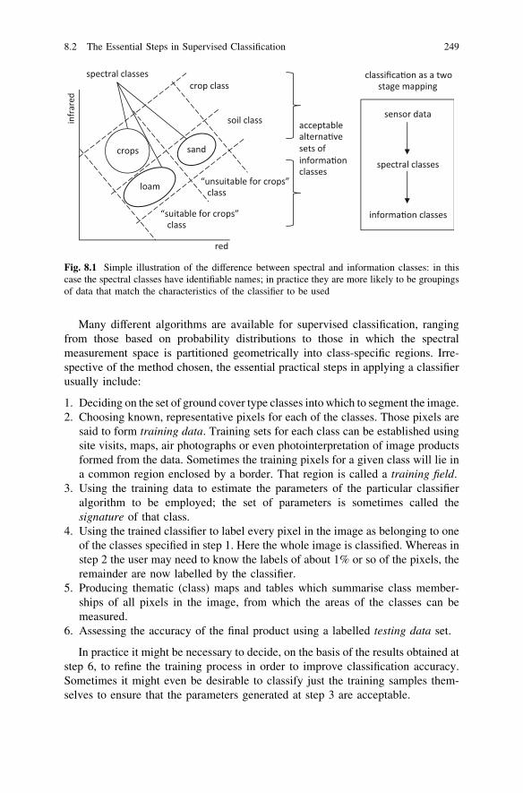
An important concept must be emphasised here, which is often overlooked inpractice and about which we will have much to say in Chap. 11. That concernswhether the classes of interest to the user occupy unique regions in spectral space,and whether there is a one-to-one mapping between the measurement vectors andclass labels. A simple illustration is shown in Fig. 8.1, which is an infrared versusvisible red spectral space of a geographical region used for growing crops. Thedata is shown to be in three moderately distinct clusters, corresponding to rich,fully growing crops (on loam), a loam soil and a sandy soil. One user might beinterested in a map of crops and soil—just two classes, but the soil class has twosub-classes—loam and sand. Another user might be interested in which parts of theregion are used to support cropping, and those that are not. The former will alsohave two sub-classes—fully growing crops and loam—but they are different fromthose of the first user. We call the classes into which the data naturally groups thespectral classes (in this simple example the crops, loam and sand) whereas thosethat match user requirements are called information classes.2

This simple example has been used to introduce the distinction. In practice thedifference may be more subtle. Spectral classes are groupings of pixel vectors inspectral space that are well matched to the particular classifier algorithm beingused. Sometimes it will be beneficial to segment even simple classes like vege-tation into sub-groups of data and let the classifier work on the sub-groups. Afterclassification is complete the analyst then maps the sub-groups to the informationclasses of interest. For most of this chapter we will not pursue any further thedistinction between the two class types. Generally, we will assume the informationand spectral classes are the same.

1 N.J. Nilsson, Learning Machines, McGraw-Hill, N.Y., 1965.2 The important distinction between information and spectral classes was first made inP.H. Swain and S.M. Davis, eds., Remote Sensing: the Quantitative Approach, McGraw-Hill,N.Y., 1978.

248 8 Supervised Classification Techniques

http://dx.doi.org/10.1007/978-3-642-30062-2_3#Fig3

http://dx.doi.org/10.1007/978-3-642-30062-2_11

Many different algorithms are available for supervised classification, rangingfrom those based on probability distributions to those in which the spectralmeasurement space is partitioned geometrically into class-specific regions. Irre-spective of the method chosen, the essential practical steps in applying a classifierusually include:

1. Deciding on the set of ground cover type classes into which to segment the image.2. Choosing known, representative pixels for each of the classes. Those pixels are

said to form training data. Training sets for each class can be established usingsite visits, maps, air photographs or even photointerpretation of image productsformed from the data. Sometimes the training pixels for a given class will lie ina common region enclosed by a border. That region is called a training field.

3. Using the training data to estimate the parameters of the particular classifieralgorithm to be employed; the set of parameters is sometimes called thesignature of that class.

4. Using the trained classifier to label every pixel in the image as belonging to oneof the classes specified in step 1. Here the whole image is classified. Whereas instep 2 the user may need to know the labels of about 1% or so of the pixels, theremainder are now labelled by the classifier.

5. Producing thematic (class) maps and tables which summarise class member-ships of all pixels in the image, from which the areas of the classes can bemeasured.

6. Assessing the accuracy of the final product using a labelled testing data set.

In practice it might be necessary to decide, on the basis of the results obtained atstep 6, to refine the training process in order to improve classification accuracy.Sometimes it might even be desirable to classify just the training samples them-selves to ensure that the parameters generated at step 3 are acceptable.

Fig. 8.1 Simple illustration of the difference between spectral and information classes: in thiscase the spectral classes have identifiable names; in practice they are more likely to be groupingsof data that match the characteristics of the classifier to be used

8.2 The Essential Steps in Supervised Classification 249

It is our objective now to consider the range of algorithms that could be used insteps 3 and 4. Recall that we are assuming that each information class consists ofjust one spectral class, unless specified otherwise, and we will use the namesinterchangeably. That allows the development of the basic algorithms to proceedwithout the added complexity of considering spectral classes, which are also calledsub-classes. Sub-classes are treated in Sect. 8.4 and in Chaps. 9 and 11.

8.3 Maximum Likelihood Classification

Maximum likelihood classification is one of the most common supervised clas-sification techniques used with remote sensing image data, and was the firstrigorous algorithm to be employed widely. It is developed in the following in astatistically acceptable manner. A more general derivation is given in Appendix E,although the present approach is sufficient for most remote sensing purposes.

8.3.1 Bayes’ Classification

Let the classes be represented by xi; i ¼ 1. . .M where M is the number of classes.In determining the class or category to which a pixel with measurement vector xbelongs, the conditional probabilities

p xijxð Þ; i ¼ 1. . . M

play a central role. The vector x is a column vector of the brightness values for thepixel in each measurement band. It describes the pixel as a point in spectral space.The probability p xijxð Þ tells us the likelihood that xi is the correct class for thepixel at position x in the spectral space. If we knew the complete set of p xijxð Þ forthe pixel, one for each class, then we could label the pixel—classify it—accordingto the decision rule

x 2 xi if p xijxð Þ[ p xjjx� �

for all j 6¼ i ð8:1Þ

This says that the pixel with measurement vector x is a member of class xi ifp xijxð Þ is the largest probability of the set. This intuitive statement is a specialcase of a more general rule in which the decisions can be biased according todifferent degrees of significance being attached to different incorrect classifica-tions. That general approach is called Bayes’ classification which is the subject ofAppendix E.

The rule of (8.1) is sometimes called a maximum posterior or MAP decisionrule, a name which will become clearer in the next section.


http://dx.doi.org/10.1007/978-3-642-30062-2_9

http://dx.doi.org/10.1007/978-3-642-30062-2_11

8.3.2 The Maximum Likelihood Decision Rule

Despite the simplicity of (8.1) the p xijxð Þ are unknown. What we can find rela-tively easily, though, are the set of class conditional probabilities p xjxið Þ; whichdescribe the chances of finding a pixel at position x in spectral space from each ofthe classes xi: Those conditional probability functions are estimated from labelledtraining data for each class. Later we will adopt a specific form for the distributionfunction, but for the moment we will retain it in general form.

The desired p xijxð Þ in (8.1) and the available p xjxið Þ; estimated from trainingdata, are related by Bayes’ theorem3

p xijxð Þ ¼ p xjxið Þ pðxiÞ=pðxÞ ð8:2Þ

in which pðxiÞ is the probability that pixels from class xi appear anywhere in theimage. If 15% of the pixels in the scene belong to class xi then we could usepðxiÞ ¼ 0:15: The pðxiÞ are referred to as prior probabilities—or sometimes justpriors. If we knew the complete set then they are the probabilities with which wecould guess the class label for a pixel before (prior to) doing any analysis. Incontrast the p xijxð Þ are the posterior probabilities since, in principle, they are theprobabilities of the class labels for a pixel at position x; after analysis. What westrive to do in statistical classification is to estimate, via (8.2), the set of classposterior probabilities for each pixel so that the pixels can be labelled according tothe largest of the posteriors, as in (8.1).

The term pðxÞ is the probability of finding a pixel with measurement vector x inthe image, from any class. Although pðxÞ is not important in the followingdevelopment it should be noted that

p xð Þ ¼XM

i¼1

pðxjxiÞpðxiÞ

On substituting from (8.2) the decision rule of (8.1) reduces to

x 2 xi if p xjxið ÞpðxiÞ[ p xjxj

� �pðxjÞ for all j 6¼ i ð8:3Þ

in which pðxÞ has been removed as a common factor, since it is not classdependent. The decision rule of (8.3) is more acceptable than that of (8.1) since thep xjxið Þ are known from training data, and it is conceivable that the priors pðxiÞare also known or can be estimated.

It is mathematically convenient now to define the discriminant function

gi xð Þ ¼ ln p xjxið Þp xið Þf g ¼ ln p xjxið Þ þ ln p xið Þ ð8:4Þ

Because the natural logarithm is a monotonic function we can substitute (8.4)directly into (8.3) to give as the decision rule:

3 J.E. Freund, Mathematical Statistics, 5th ed., Prentice Hall, N.J., 1992.

8.3 Maximum Likelihood Classification 251

x 2 xi if gi xð Þ[ gj xð Þ for all j 6¼ i ð8:5Þ

8.3.3 Multivariate Normal Class Models

To develop the maximum likelihood classifier further we now choose a particularprobability model for the class conditional density function p xjxið Þ: The mostcommon choice is to assume p xjxið Þ is a multivariate normal distribution, alsocalled a Gaussian distribution. This tacitly assumes that the classes of pixels ofinterest in spectral space are normally distributed. That is not necessarily ademonstrable property of natural spectral or information classes, but the Gaussianis a simple distribution to handle mathematically and its multivariate properties arewell known. For an N dimensional space the specific form of the multivariateGaussian distribution function is4

p xjxið Þ ¼ ð2pÞ�N=2 Cij j�1=2exp � 1=2ðx�miÞTC�1

i x�mið Þn o

ð8:6Þ

where mi and Ci are the mean vector and covariance matrix of the data in class xi:We will sometimes write the normal distribution in the shorthand formNðxjmi;CiÞ:

Substituting (8.6) into (8.4) gives the discriminant function

gi xð Þ ¼ �1=2Nln2p� 1=2 ln jCij � 1=2ðx�miÞTC�1i x�mið Þ þ ln pðxiÞ

Since the first term is not class dependent is doesn’t aid discrimination and can beremoved, leaving as the discriminant function

gi xð Þ ¼ ln pðxiÞ � 1=2 ln jCij � 1=2ðx�miÞTC�1i x�mið Þ ð8:7Þ

If the analyst has no useful information about the values of the prior probabilitiesthey are assumed all to be equal. The first term in (8.7) is then ignored, allowingthe 1=2 to be removed as well, leaving

gi xð Þ ¼ � ln jCij � ðx�miÞTC�1i x�mið Þ ð8:8Þ

which is the discriminant function for the Gaussian maximum likelihood classifier,so-called because it essentially determines class membership of a pixel based onthe highest of the class conditional probabilities, or likelihoods. Its implementationrequires use of either (8.7) or (8.8) in (8.5). There is an important practical con-sideration concerning whether all the classes have been properly represented in thetraining data available. Because probability distributions like the Gaussian existover the full domain of their argument (in this case the spectral measurements) useof (8.5) will yield a class label even in the remote tails of the distribution functions.In Sect. 8.3.5 the use of thresholds allows the user to avoid such inappropriatelabelling and thereby to identify potentially missing classes.

4 See Appendix D.


8.3.4 Decision Surfaces

The probability distributions in the previous section have been used to discriminateamong the candidate class labels for a pixel. We can also use that material to seehow the spectral space is segmented into regions corresponding to the classes. Thatrequires finding the shapes of the separating boundaries in vector space. As willbecome evident, an understanding of the boundary shapes will allow us to assessthe relative classification abilities, or strengths, of different classifiers.

Spectral classes are defined by those regions in spectral space where theirdiscriminant functions are the largest. Those regions are separated by surfaceswhere the discriminant functions for adjoining spectral classes are equal. The ithand jth spectral classes are separated by the surface

gi xð Þ � gj xð Þ ¼ 0

which is the actual equation of the surface. If all such surfaces were known thenthe class membership of a pixel can be made on the basis of its position in spectralspace relative to the set of surfaces.

The construction ðx�miÞTC�1i x�mið Þ in (8.7) and (8.8) is a quadratic

function of x: Consequently, the decision surfaces generated by Gaussian maxi-mum likelihood classification are quadratic and thus take the form of parabolas,ellipses and circles in two dimensions, and hyperparaboloids, hyperellipsoids andhyperspheres in higher dimensions.

8.3.5 Thresholds

It is implicit in the rule of (8.1) and (8.5) that pixels at every point in spectral spacewill be classified into one of the available classes xi; irrespective of how small theactual probabilities of class membership are. This is illustrated for one dimensionaldata in Fig. 8.2a. Poor classification can result as indicated. Such situations canarise if spectral classes have been overlooked or, if knowing other classes existed,enough training data was not available to estimate the parameters of their distri-butions with any degree of accuracy (see Sect. 8.3.6 following).

In situations such as those it is sensible to apply thresholds to the decisionprocess in the manner depicted in Fig. 8.2b. Pixels which have probabilities for allclasses below the threshold are not classified. In practice, thresholds are applied tothe discriminant functions and not the probability distributions, since the latter arenever actually computed. With the incorporation of a threshold the decision rule of(8.5) becomes

x 2 xi if gi xð Þ[ gj xð Þ for all j 6¼ i ð8:9aÞ

and gi xð Þ[ Ti ð8:9bÞ


where Ti is the threshold to be used on class xi:We now need to understand how a reasonable value for Ti can be chosen.

Substituting (8.7) into (8.9b) gives

ln pðxiÞ � 1=2 ln jCij � 1=2ðx�miÞTC�1i x�mið Þ[ Ti

or

ðx�miÞTC�1i x�mið Þ\� 2Ti þ 2 ln pðxiÞ � ln jCij ð8:10Þ

If x is normally distributed, the expression on the left hand side of (8.10) has a v2

distribution with N degrees of freedom,5 where N is the number of bands in thedata. We can, therefore, use the properties of the v2 distribution to determine that

value of ðx�miÞTC�1i x�mið Þ below which a desired percentage of pixels will

Fig. 8.2 Illustration of the use of thresholds to avoid questionable classification decisions

5 See Swain and Davis, loc. cit.


exist. Larger values of ðx�miÞTC�1i x�mið Þ correspond to pixels lying further

out in the tails of the normal distribution. That is shown in Fig. 8.3.As an example of how this is used consider the need to choose a threshold such

that 95% of all pixels in a class will be classified, or such that the 5% least likelypixels for the class will be rejected. From the v2 distribution we find that 95% ofall pixels have v2 values below 9.488. Thus, from (8.10)

Ti ¼ �4:744þ ln pðxiÞ � 1=2 ln jCij

which can be calculated from a knowledge of the prior probability and covariancematrix for the ith spectral class.

8.3.6 Number of Training Pixels Required

Enough training pixels for each spectral class must be available to allow reason-able estimates to be obtained of the elements of the class conditional mean vectorand covariance matrix. For an N dimensional spectral space the mean vector has Nelements. The covariance matrix is symmetric of size N � N; it has 1=2 NðN þ 1Þdistinct elements that need to be estimated from the training data. To avoid thematrix being singular, at least NðN þ 1Þ independent samples are needed. Fortu-nately, each N dimensional pixel vector contains N samples, one in each wave-band; thus the minimum number of independent training pixels required isðN þ 1Þ: Because of the difficulty in assuring independence of the pixels, usuallymany more than this minimum number are selected. A practical minimum of 10Ntraining pixels per spectral class is recommended, with as many as 100N per classif possible.6 If the covariance matrix is well estimated then the mean vector will bealso, because of its many fewer elements.

Fig. 8.3 Use of the v2

distribution for obtainingclassifier thresholds

6 See Swain and Davis, loc. cit., although some authors regard this as a conservatively highnumber of samples.


For data with low dimensionality, say up to 10 bands, 10N to 100N can usuallybe achieved, but for higher order data sets, such as those generated by hyper-spectral sensors, finding enough training pixels per class is often not practical,making reliable training of the traditional maximum likelihood classifier difficult.In such cases, dimensionality reduction procedures can be used, including methodsfor feature selection. They are covered in Chap. 10.

Another approach that can be adopted when not enough training samples areavailable is to use a classification algorithm with fewer parameters, several ofwhich are treated in later sections. It is the need to estimate all the elements of thecovariance matrix that causes problems for the maximum likelihood algorithm.The minimum distance classifier, covered in Sect. 8.5, depends only on knowingthe mean vector for each training class—consequently there are only N unknownsto estimate.

8.3.7 The Hughes Phenomenon and the Curse of Dimensionality

Although recognised as a potential problem since the earliest application ofcomputer-based interpretation to remotely sensed imagery, the Hughes phenom-enon had not been a significant consideration until the availability of hyperspectraldata. It concerns the number of training samples required per class to train asupervised classifier reliably and is thus related to the material of the previoussection. Although that was focussed on Gaussian maximum likelihood classifi-cation, in principle any classifier that requires parameters to be estimated is subjectto the problem.7 It manifests itself in the following manner.

Clearly, if too few samples are available good estimates of the class parameterscannot be found; the classifier will not be properly trained and will not predict wellon data from the same classes that it has not already seen. The extent to which aclassifier predicts on previously unseen data, referred to as testing data, is calledgeneralisation. Increasing the set of random training samples would be expected toimprove parameter estimates, which indeed is generally the case, and thus lead tobetter generalisation.

Suppose now we have enough samples for a given number of dimensions toprovide reliable training and good generalisation. Instead of changing the numberof training samples, imagine now we can add more features, or dimensions, to theproblem. On the face of it that suggests that the results should be improvedbecause more features should bring more information into the training phase.However, if we don’t increase the number of training samples commensurately wemay not be able to get good estimates of the larger set of parameters created by the

7 See M. Pal and G.F. Foody, Feature selection for classification of hyperspectral data for SVM,IEEE Transactions on Geoscience and Remote Sensing, vol. 48, no. 5, May 2010, pp. 2297–2307for a demonstration of the Hughes phenomenon with the support vector machine of Sect. 8.14.


http://dx.doi.org/10.1007/978-3-642-30062-2_10

increased dimensionality, and both training and generalisation will suffer. That isthe essence of the Hughes phenomenon.

The effect of poorly estimated parameters resulting from too few trainingsamples with increased dimensionality was noticed very early in the history ofremote sensing image classification. Figure 8.4 shows the results of a five classagricultural classification using 12 channel aircraft scanner data.8 Classificationaccuracy is plotted as a function of the number of features (channels) used. Asnoted, when more features are added there is an initial improvement in classifi-cation accuracy until such time as the estimated maximum likelihood statisticsapparently become less reliable.

As another illustration consider the determination of a reliable linear separatingsurface; here we approach the problem by increasing the number of training samplesfor a given dimensionality, but the principle is the same. Figure 8.5 shows threedifferent training sets of data for the same two dimensional data set. The first has onlyone training pixel per class, and thus the same number of training pixels as dimensions.As seen, while a separating surface can be found it may not be accurate. The classifierperforms at the 100% level on the training data but is very poor on testing data.

Having two training pixels per class, as in the case of the middle diagram,provides a better estimate of the separating surface, but it is not until we havemany pixels per class compared to the number of channels, as in the right handfigure, that we obtain good estimates of the parameters of the supervised classifier,so that generalisation is good.

Fig. 8.4 Actual experimental classification results showing the Hughes phenomenon—the lossof classification accuracy as the dimensionality of the spectral domain increases

8 Based on results presented in K.S. Fu, D.A. Landgrebe and T.L. Phillips, Information processingof remotely sensed agricultural data, Proc. IEEE, vol. 57, no. 4, April 1969, pp. 639–653.


The Hughes phenomenon was first examined in 19689 and has become widelyrecognised as a major consideration whenever parameters have to be estimated in ahigh dimensional space. In the field of pattern recognition it is often referred to asthe curse of dimensionality.10

8.3.8 An Example

As a simple example of the maximum likelihood approach, the 256 9 276 pixelsegment of Landsat Multispectral Scanner image shown in Fig. 8.6 is to beclassified. Four broad ground cover types are evident: water, fire burn, vegetationand urban. Assume we want to produce a thematic map of those four cover types inorder to enable the distribution of the fire burn to be evaluated.

The first step is to choose training data. For such a broad classification, suitablesets of training pixels for each of the four classes are easily identified visually inthe image data. The locations of four training fields for this purpose are seen insolid colours on the image. Sometimes, to obtain a good estimate of class statisticsit may be necessary to choose several training fields for each cover type, located indifferent regions of the image, but that is not necessary in this case.

The signatures for each of the four classes, obtained from the training fields, aregiven in Table 8.1. The mean vectors can be seen to agree generally with theknown spectral reflectance characteristics of the cover types. Also, the classvariances, given by the diagonal elements in the covariance matrices, are small forwater as might be expected but on the large side for the developed/urban class,indicative of its heterogeneous nature.

Fig. 8.5 Estimating a linear separating surface using an increasing number of training samples,showing poor generalisation if too few per number of features are used; the dashed curverepresents the optimal surface

9 G. F Hughes, On the mean accuracy of statistical pattern recognizers, IEEE Transactions onInformation Theory, vol. IT-14, no.1, 1968, pp. 55–63.10 C.M. Bishop, Pattern Recognition and Machine Learning, Springer Science ? BusinessMedia, LLC, N.Y., 2006.


When used in a maximum likelihood algorithm to classify the four bands of theimage in Fig. 8.6, the signatures generate the thematic map of Fig. 8.7. The fourclasses, by area, are given in Table 8.2. Note that there are no unclassified pixels,since a threshold was not used in the labelling process. The area estimates areobtained by multiplying the number of pixels per class by the effective area of apixel. In the case of the Landsat multispectral scanner the pixel size is 0.4424hectare.

Table 8.1 Class signaturesgenerated from the trainingareas in Fig. 8.6

Class Meanvector

Covariance matrix

Water 44.27 14.36 9.55 4.49 1.1928.82 9.55 10.51 3.71 1.1122.77 4.49 3.71 6.95 4.0513.89 1.19 1.11 4.05 7.65

Fire burn 42.85 9.38 10.51 12.30 11.0035.02 10.51 20.29 22.10 20.6235.96 12.30 22.10 32.68 27.7829.04 11.00 20.62 27.78 30.23

Vegetation 40.46 5.56 3.91 2.04 1.4330.92 3.91 7.46 1.96 0.5657.50 2.04 1.96 19.75 19.7157.68 1.43 0.56 19.71 29.27

Urban 63.14 43.58 46.42 7.99 -14.8660.44 46.42 60.57 17.38 -9.0981.84 7.99 17.38 67.41 67.5772.25 -14.86 -9.09 67.57 94.27

Fig. 8.6 Image segment tobe classified, consisting of amixture of natural vegetation,waterways, urban regions,and vegetation damaged byfire. Four training areas areidentified in solid colour.They are water (violet),vegetation (green), fire burn(red) and urban (dark blue inthe bottom right handcorner). Those pixels wereused to generate thesignatures in Table 8.1


8.4 Gaussian Mixture Models

In order that the maximum likelihood classifier algorithm work effectively it isimportant that the classes be as close to Gaussian as possible. In Sect. 8.2 that wasstated in terms of knowing the number of spectral classes, sometimes also referredto as modes or sub-classes, of which each information class is composed. In Chap.11 we will employ the unsupervised technique of clustering, to be developed in thenext chapter, to help us do that. Here we present a different approach, based on theassumption that the image data is composed of a set of Gaussian distributions,some subsets of which may constitute information classes. This material isincluded at this point because it fits logically into the flow of the chapter, but it is alittle more complex and could be passed over on a first reading.11

We commence by assuming that the pixels in a given image belong to a prob-ability distribution that is a linear mixture of K Gaussian distributions of the form

p xð Þ ¼XK

k¼1

akNðxjmk;CkÞ ð8:11Þ

The ak are a set of mixture proportions, which are also considered to be the priorprobabilities of each of the components that form the mixture. They satisfy

0� ak � 1 ð8:12aÞ

Fig. 8.7 Thematic mapproduced using the maximumlikelihood classifier; bluerepresents water, red is firedamaged vegetation, green isnatural vegetation and yellowis urban development

Table 8.2 Tabular summaryof the thematic map ofFig. 8.7

Class Number of pixels Area (ha)

Water 4,830 2,137Fire burn 14,182 6,274Vegetation 28,853 12,765Urban 22,791 10,083

11 A very good treatment of Gaussian mixture models will be found in C.M. Bishop, loc. cit.


http://dx.doi.org/10.1007/978-3-642-30062-2_11

http://dx.doi.org/10.1007/978-3-642-30062-2_11

and

XK

k¼1

ak ¼ 1 ð8:12bÞ

Equation (8.11) is the probability of finding a pixel at position x in spectral spacefrom the mixture. It is the mixture equivalent of the probability p xjxið Þ of finding apixel at position x from the single class xi: Another way of writing the expressionfor the class conditional probability for a single distribution is p xjmi;Cið Þ; in whichthe class has been represented by its parameters—the mean vector and covariancematrix—rather than by class label itself. Similarly, p xð Þ in the mixture equationabove could be shown as conditional on the parameters of the mixture explicitly, viz.

p xjak;mK;CKð Þ ¼XK

k¼1

akNðxjmk;CkÞ ð8:13Þ

in which mK is the set of all K mean vectors, CK is the set of all K covariancematrices and aK is the set of mixture parameters.

What we would like to do now is find the parameters in (8.13) that give the bestmatch of the model to the data available. In what follows we assume we know, orhave estimated, the number of components K; what we then have to find are thesets of mean vectors, covariance matrices and mixture proportions.

Suppose we have available a data set of J pixels X ¼ fx1. . .xJg assumed to beindependent samples from the mixture. Their joint likelihood can be expressed

p Xjak;mK;CKð Þ ¼YJ

j¼1

p xjjak;mK;CK

� �

the logarithm12 of which is

ln p Xjak;mK;CKð Þ ¼XJ

j¼1

ln p xjjak;mK;CK

� �ð8:14Þ

We now want to find the parameters that will maximise the log likelihood that Xcomes from the mixture. In other words we wish to maximise (8.14) with respectto the members of the sets mK ¼ fmk; k ¼ 1. . .Kg; CK ¼ fCk; k ¼ 1. . .Kg;aK ¼ fak; k ¼ 1. . .Kg: Substituting (8.13) in (8.14) we have

ln p Xjak;mK;CKð Þ ¼XJ

j¼1

lnXK

k¼1

akNðxjjmk;CkÞ ð8:15Þ

12 As in Sect. 8.3, using the logarithmic expression simplifies the analysis to follow.

8.4 Gaussian Mixture Models 261

Differentiating this with respect to the mean vector of, say, the kth component, andequating the result to zero gives

XJ

j¼1

o

omklnXK

k¼1

akNðxjjmk;CkÞ ¼ 0

XJ

j¼1

1PK

k¼1 akNðxjjmk;CkÞo

omk

XK

k¼1

akNðxjjmk;CkÞ ¼ 0 ð8:16Þ

XJ

j¼1

akNðxjjmk;CkÞPK


omk�1=2ðxj �mkÞTC�1

k xj �mk

� �n o¼ 0

Using the matrix property13 oox xT Axf g ¼ 2Ax this can be written

XJ

j¼1

ak pðxjjmk;CkÞp xjjak;mK;CK

� �C�1k xj �mk

� ��XJ

j¼1

ak pðxjjmk;CkÞp xj

� � C�1k xj �mk

� �¼ 0

If we regard ak as the prior probability of the kth component then the fraction justinside the sum will be recognised, from Bayes’ Theorem, as pðmk;CkjxjÞ, theposterior probability for that component given the xjth sample,14 so that the lastequation becomes

XJ

j¼1

pðmk;CkjxjÞC�1k xj �mk

� �¼ 0

The inverse covariance matrix cancels out; rearranging the remaining terms gives

mk ¼PJ

j¼1 pðmk;CkjxjÞxjPJ

j¼1 pðmk;CkjxjÞ

The posterior probabilities in the denominator, p mk;Ckjxj

� �; express the likeli-

hood that the correct component is k for the sample xj: It would be high if thesample belongs to that component, and low otherwise. The sum over all samples ofthe posterior probability for component k in the denominator is a measure of theeffective number of samples likely to belong to that component,15 and we define itas Nk:

13 See K.B. Petersen and M.S. Pedersen, The Matrix Cookbook, 14 Nov 2008, http://matrixcookbook.com14 In C.M. Bishop, loc. cit., it is called the responsibility.15 See Bishop, loc. cit.


http://matrixcookbook.com

http://matrixcookbook.com

Nk ¼XJ

j¼1

pðmk;CkjxjÞ ð8:17Þ

Note that the numerator in the expression for mk above is a sum over all thesamples weighted by how likely it is that the kth component is the correct one ineach case. The required values of the mk that maximise the log likelihood in (8.15)can now be written

mk ¼1

Nk

XJ

j¼1

pðmk;CkjxjÞxj ð8:18Þ

To find the covariance matrices of the components that maximise (8.15) we pro-ceed in a similar manner by taking the first derivative with respect to Ck andequating the result to zero. Proceeding as before we have, similar to (8.16),

XJ

j¼1

akPK


oCkNðxjjmk;CkÞ ¼ 0 ð8:19Þ

The derivative of the normal distribution with respect to its covariance matrix is alittle tedious but relatively straightforward in view of two more useful matrixcalculus properties16:

o

oMMj j ¼ Mj jðM�1ÞT ð8:20aÞ

o

oMaTM�1a ¼ �ðM�1ÞTaaTðM�1ÞT ð8:20bÞ

Using these we find

o

oCkNðxjjmk;CkÞ ¼ N xjjmk;Ck

� �ðxj �mkÞðxj �mkÞTðC�1

k ÞT � 1

n o

When substituted in (8.19) this gives

XJ

j¼1

akN xjjmk;Ck

� �

PKk¼1 akNðxjjmk;CkÞ

ðxj �mkÞðxj �mkÞTðC�1k Þ

T � 1n o

¼ 0

Recognising as before that the fraction just inside the summation is the posteriorprobability, and multiplying throughout by C�1

k ; and recalling that the covariancematrix is symmetric, we have

16 See K.B. Petersen and M.S. Pedersen, loc. cit.


XJ

j¼1

pðmk;CkjxjÞ ðxj �mkÞðxj �mkÞT � Ck

n o¼ 0

so that, with (8.17), this gives

Ck ¼1

Nk

XJ

j¼1

pðmk;CkjxjÞ ðxj �mkÞðxj �mkÞTn o

ð8:21Þ

which is the expression for the covariance matrix of the kth component that willmaximise (8.15). Note how similar this is in structure to the covariance matrixdefinition for a single Gaussian component in (6.3). In (8.21) the terms are sum-med with weights that are the likelihoods that the samples come from the kthcomponent. If there were only one component then the weight would be unity,leading to (6.3).

The last task is to find the mixing parameter of the kth component that con-tributes to maximising the log likelihood of (8.15). The ak are also constrained by(8.12b). Therefore we maximise the following expression with respect to ak usingLagrange multipliers k to constrain the maximisation17:

XJ

j¼1

lnXK

k¼1

akNðxjjmk;CkÞ þ kXK

k¼1

ak � 1

( )

Putting the first derivative with respect to ak to zero gives

XJ

j¼1

Nðxjjmk;CkÞPKk¼1 akNðxjjmk;CkÞ

þ k ¼ 0

which, using (8.13), is

XJ

j¼1

Nðxjjmk;CkÞp xjjak;mK;CK

� �þ k ¼ 0

and, using Bayes’ Theorem

XJ

j¼1

p mk;Ckjxj

� �

akþ k ¼ 0

Multiplying throughout by ak and using (8.17) this gives

Nk þ akk ¼ 0 ð8:22Þ

17 For a good treatment of Lagrange multipliers see C.M. Bishop, loc. cit., Appendix E


http://dx.doi.org/10.1007/978-3-642-30062-2_6

http://dx.doi.org/10.1007/978-3-642-30062-2_6

so that if we take the sumXK

k¼1

Nk þ akkf g ¼ 0

we have, in view of (8.12b) k ¼ �N

Thus, from (8.22), ak ¼Nk

Nð8:23Þ

With (8.18), (8.21) and (8.23) we now have expressions for the parameters of theGaussian mixture model that maximise the log likelihood function of (8.14).Unfortunately, though, they each depend on the posterior probabilitiespðmk;CkjxjÞ which themselves are dependent on the parameters. The results of(8.18), (8.21) and (8.23) do not therefore represent solutions to the Gaussianmixing problem. However, an iterative procedure is available that allows theparameters and the posteriors to be determined progressively. It is called Expec-tation–Maximisation (EM) and is outlined in the algorithm of Table 8.3. It consistsof an initial guess for the parameters, following which values for the posteriors arecomputed—that is called the expectation step. Once the posteriors have beencomputed, new estimates for the parameters are computed from (8.18), (8.21) and(8.23). That is the maximisation step. The loop is repeated until the parametersdon’t change any further. It is also helpful at each iteration to estimate the loglikelihood of (8.14) and use it to check convergence.

8.5 Minimum Distance Classification

8.5.1 The Case of Limited Training Data

The effectiveness of maximum likelihood classification depends on reasonablyaccurate estimation of the mean vector m and the covariance matrix C for eachspectral class. This in turn depends on having a sufficient number of training pixelsfor each of those classes. In cases where that is not possible, inaccurate estimatesof the elements of C result, leading to poor classification.

When the number of training samples per class is limited it may sometimes bemore effective to resort to an algorithm that does not make use of covarianceinformation but instead depends only on the mean positions of the spectral classes,noting that for a given number of samples they can be more accurately estimatedthan covariances. The minimum distance classifier, or more precisely, minimumdistance to class means classifier, is such an approach. With this algorithm,training data is used only to determine class means; classification is thenperformed by placing a pixel in the class of the nearest mean.


The minimum distance algorithm is also attractive because it is faster thanmaximum likelihood classification, as will be seen in Sect. 8.5.6. However,because it does not use covariance data it is not as flexible. In maximum likelihoodclassification each class is modelled by a multivariate normal class model that canaccount for spreads of data in particular spectral directions. Since covariance datais not used in the minimum distance technique class models are symmetric in thespectral domain. Elongated classes will, therefore, not be well modelled. Insteadseveral spectral classes may need to be used with this algorithm in cases where onemight be suitable for maximum likelihood classification.

Table 8.3 The Expectation–Maximisation Algorithm for Mixtures of Gaussians

Step 1: Initialisation Choose initial values for ak;mk;Ck:

Call these aoldk ;mold

k ;Coldk

Step 2: Expectation Evaluate the posterior probabilities using the current estimates forak;mk;Ck; according to:

p mk;Ckjxj

� �¼

aoldk p xjjmold

k ;Coldk

� �

p xjjaoldK ;mold

K ;ColdK

� �

i.e.

p mk;Ckjxj

� �¼

aoldk p xjjmold

k ;Coldk

� �

PKk¼1 aold

k Nðxjjmoldk ;Cold

k Þ

Step 3: Maximisation Compute new values for ak;mk;Ck from (8.18), (8.21)and (8.23) in the following way:First compute

Nk ¼PJ

j¼1pðmold

k ;Coldk jxjÞ

then

mnewk ¼ 1

Nk

XJ

j¼1

pðmoldk ;Cold

k jxjÞxj

Cnewk ¼ 1

Nk

XJ

j¼1

pðmoldk ;Cold

k jxjÞfðxj �mnewk Þðxj �mnew

k ÞTg

anewk ¼ Nk

NAlso, evaluate the log likelihood

ln p Xjak;mK;CKð Þ ¼PJ

j¼1lnPK

k¼1aold

k Nðxjjmoldk ;Cold

k Þ

Step 4: Evaluation If mnewk � mold

k ; Cnewk � Cold

k ; anewk � aold

k

then terminate the process. Otherwise put

moldk ¼ mnew

k ; Coldk ¼ Cnew

k ; aoldk ¼ anew

k

and return to Step 2.This check can also be carried out on the basis of little or no changein the log likelihood calculation


8.5.2 The Discriminant Function

Suppose mi; i ¼ 1. . .M are the means of the M classes determined from trainingdata, and x is the position of the pixel in spectral space to be classified. Compute theset of squared Euclidean distances of the unknown pixel to each of the class means:

dðx;miÞ2 ¼ ðx�miÞT x�mið Þ ¼ ðx�miÞ � x�mið Þ i ¼ 1. . .M

Expanding the dot product form gives

dðx;miÞ2 ¼ x � x� 2mi � xþmi �mi

Classification is performed using the decision rule

x 2 xi if dðx;miÞ2\ dðx;mjÞ2 for all j 6¼ i

Since x � x is common to all squared distance calculations it can be removed fromboth sides in the decision rule. The sign of the remainder can then be reversed sothat the decision rule can be written in the same way as (8.5) to give

x 2 xi if gi xð Þ[ gj xð Þ for all j 6¼ i

in which gi xð Þ ¼ 2mi � x�mi �mi ð8:24Þ

Equation (8.24) is the discriminant function for the minimum distance classifier.18

8.5.3 Decision Surfaces for the Minimum Distance Classifier

The implicit surfaces in spectral space separating adjacent classes are defined bythe respective discriminant functions being equal. The surface between the ith andjth spectral classes is given by

gi xð Þ � gj xð Þ ¼ 0

which, when substituting from (8.24), gives

2 mi �mj

� �� x� mi �mi �mj �mj

� �¼ 0

This defines a linear surface, called a hyperplane in more than three dimensions.The surfaces between each pair of classes define a set of first degree separatinghyperplanes that partition the spectral space linearly. The quadratic decision

18 It is possible to implement a minimum distance classifier using distance measures other thanEuclidean: see A.G. Wacker and D.A. Landgrebe, Minimum distance classification in remotesensing, First Canadian Symposium on Remote Sensing, Ottawa, 1972.

8.5 Minimum Distance Classification 267

surface generated by the maximum likelihood rule in Sect. 8.3.4 renders thatalgorithm potentially more powerful than the minimum distance rule if properlytrained; the minimum distance classifier nevertheless is effective when the numberof training samples is limited or if linear separation of the classes is suspected.

8.5.4 Thresholds

Thresholds can be applied to minimum distance classification by ensuring not onlythat a pixel is closest to a candidate class but also that it is within a prescribeddistance of that class in spectral space. Such an assessment is often used with theminimum distance rule. The distance threshold is usually specified in terms of anumber of standard deviations from the class mean.

8.5.5 Degeneration of Maximum Likelihood to MinimumDistance Classification

The major difference between the minimum distance and maximum likelihoodclassifiers lies in the use, by the latter, of the sample covariance information.Whereas the minimum distance classifier labels a pixel as belonging to a particularclass on the basis only of its distance from the relevant mean in spectral space,irrespective of its direction from that mean, the maximum likelihood classifiermodulates its decision with direction, based on the information contained in thecovariance matrix. Furthermore, the entry 1=2 lnjCij in its discriminant functionshows explicitly that patterns have to be closer to some means than others to haveequivalent likelihoods of class membership. As a result, superior performance isexpected of the maximum likelihood classifier. The following situation howeverwarrants consideration since there is then no advantage in maximum likelihoodprocedures. It could occur in practice when class covariance is dominated bysystematic noise rather than by the natural spectral spreads of the individualspectral classes.

Consider the covariance matrices of all classes to be diagonal and equal, and thevariances in each component to be identical, so that

Ci ¼ r2I for all i

in which I is the identity matrix. The discriminant function for the maximumlikelihood classifier in (8.7) then becomes

gi xð Þ ¼ �1=2lnr2N � 12r2ðx�miÞT x�mið Þ þ lnpðxiÞ


The first term on the right hand side is common to all discriminant functions andcan be ignored. The second term can be expanded in dot product form in which theresulting x � x terms can also be ignored, leaving

gi xð Þ ¼ 12r2ð2mi � x�mi �miÞ þ lnpðxiÞ

If all the prior probabilities are assumed to be equal then the last term can beignored, allowing 1=2r2 to be removed as a common factor, leaving

gi xð Þ ¼ 2mi � x�mi �mi

which is the same as (8.24), the discriminant function for the minimum distanceclassifier. Therefore, minimum distance and maximum likelihood classification arethe same for identical and symmetric spectral class distributions.

8.5.6 Classification Time Comparison of the MaximumLikelihood and Minimum Distance Rules

For the minimum distance classifier the discriminant function in (8.24) must beevaluated for each pixel and each class. In practice 2mi and mi �mi would becalculated beforehand, leaving the computation of N multiplications and N addi-tions to check the potential membership of a pixel to one class, where N is thenumber of components in x. By comparison, evaluation of the discriminantfunction for maximum likelihood classification in (8.7) requires N2 þ N multi-plications and N2 þ 2N þ 1 additions to check a pixel against one class, given thatln pðxiÞ � 1=2 ln jCij would have been calculated beforehand. Ignoring additions bycomparison to multiplications, the maximum likelihood classifier takes N þ 1times as long as the minimum distance classifier to perform a classification. It isalso significant to note that classification time, and thus cost, increases quadrati-cally with the number of spectral components for the maximum likelihood clas-sifier, but only linearly for minimum distance classification.

8.6 Parallelepiped Classification

The parallelepiped classifier is a very simple supervised classifier that is trained byfinding the upper and lower brightness values in each spectral dimension. Oftenthat is done by inspecting histograms of the individual spectral components in theavailable training data, as shown in Fig. 8.8. Together the upper and lower boundsin each dimension define a multidimensional box or parallelepiped; Fig. 8.9 showsa set of two dimensional parallelepipeds. Unknown pixels are labelled as comingfrom the class of the parallelepiped within which they lie.

8.5 Minimum Distance Classification 269

While it is a very simple, and fast, classifier, it has several limitations. First,there can be considerable gaps between the parallelepipeds in spectral space;pixels in those regions cannot be classified. By contrast, the maximum likelihoodand minimum distance rules will always label unknown pixels unless thresholdsare applied. Secondly, for correlated data some parallelepipeds can overlap, asillustrated in Fig. 8.10, because their sides are always parallel to the spectral axes.

Fig. 8.8 Setting the parallelepiped boundaries by inspecting class histograms in each band

Fig. 8.9 A set of twodimensional parallelepipeds

Fig. 8.10 Classification ofcorrelated data showingregions of inseparability


As a result, there are some parts of the spectral domain that can’t be separated.Finally, as with the minimum distance classifier, there is no provision for priorprobability of class membership with the parallelepiped rule.

8.7 Mahalanobis Classification

Consider the discriminant function for the maximum likelihood classifier for thespecial case of equal prior probabilities in (8.8). If the sign is reversed the functioncan be considered as a distance squared measure because the quadratic entry hasthose dimensions and the other term is a constant. Thus we can define

d x;mið Þ2¼ ln jCij þ ðx�miÞTC�1i x�mið Þ ð8:25Þ

and classify an unknown pixel on the basis of the smallest dðx;miÞ; as for theEuclidean minimum distance classifier. Thus the maximum likelihood classifier(with equal priors) can be considered as a minimum distance algorithm but with adistance measure that is sensitive to direction in spectral space.

Assume now that all class covariances are the same and given by Ci ¼ C for alli. The ln jCj term is now not discriminating and can be ignored. The squareddistance measure then reduces to

d x;mið Þ2¼ ðx�miÞTC�1 x�mið Þ ð8:26Þ

A classifier using this simplified distance measure is called a Mahalanobis clas-sifier and the distance measure shown squared in (8.26) is called the Mahalanobisdistance. Under the additional simplification of C ¼ r2I the Mahalanobis classifierreduces to the minimum Euclidean distance classifier of Sect. 8.5.

The advantage of the Mahalanobis classifier over the maximum likelihoodprocedure is that it is faster and yet retains a degree of direction sensitivity via thecovariance matrix C; which could be a class average or a pooled covariance.

8.8 Non-parametric Classification

Classifiers such as the maximum likelihood and minimum distance rules are oftencalled parametric because the class definitions and discriminant functions aredefined in terms of sets of parameters, such as the mean vectors and covariancematrices for each class.

One of the valuable aspects of the parametric, statistical approach is that a set ofrelative likelihoods is produced. Even though, in the majority of cases, the max-imum of the likelihoods is chosen to indicate the most probable label for a pixel,there exists nevertheless information in the remaining likelihoods that could bemade use of in some circumstances, either to initiate processes such as relaxation

8.6 Parallelepiped Classification 271

labelling (Sect. 8.20.4) and Markov random fields (Sect. 8.20.5) or simply toprovide the user with some feeling for the other likely classes. Those situations arenot common however and, in most remote sensing applications, the maximumselection is made. That being so, the material in Sects. 8.3.4 and 8.5.3 shows thatthe decision process has a geometric counterpart in that a comparison of statisti-cally derived discriminant functions leads equivalently to a decision rule thatallows a pixel to be classified on the basis of its position in spectral space com-pared with the location of a decision surface.

There are also classifiers that, in principle, don’t depend on parameter sets andare thus called non-parametric. Two simple non-parametric methods are given inSects. 8.9 and 8.10, although the table look up approach of Sect. 8.9 is now rarelyused.

Non-parametric methods based on finding geometric decision surfaces werepopular in the very early days of pattern recognition19 but fell away over the 1980sand 1990s because flexible training algorithms could not be found. They have,however, been revived in the past two decades with the popularity of the supportvector classifier and the neural network, which we treat in Sects. 8.14 and 8.19respectively, after we explore the fundamental problems with non-parametricapproaches.

8.9 Table Look Up Classification

Since the set of discrete brightness values that can be taken by a pixel in eachspectral band is limited by the radiometric resolution of the data, there is a finite,although often very large, number of distinct pixel vectors in any particular image.For a given class there may not be very many different pixel vectors if theradiometric resolution is not high, as was the case with the earliest remote sensinginstruments. In such situations a viable classification scheme is to note the set ofpixel vectors corresponding to a given class based on representative training data,and then use those vectors to classify the image by comparing unknown pixelswith each pixel in the training data until a match is found. No arithmetic operationsare required and, notwithstanding the number of comparisons that might benecessary to determine a match, it is a fast classifier. It is referred to as a look uptable approach since the training pixel brightnesses are stored in tables that pointto the corresponding classes.

An obvious drawback with this technique is that the chosen training data mustcontain an example of every possible pixel vector for each class. Should some bemissed then the corresponding pixels in the image will be left unclassified. Withmodern data sets, in which there can be billions of individual data vectors, thisapproach is impractical.

19 See N.J. Nilsson, Learning Machines, McGraw-Hill, N.Y., 1965.


8.10 kNN (Nearest Neighbour) Classification

A classifier that is particularly simple in concept, but can be time consuming toapply, is the k Nearest Neighbour classifier. It assumes that pixels close to eachother in spectral space are likely to belong to the same class. In its simplest forman unknown pixel is labelled by examining the available training pixels in thespectral domain and choosing the class most represented among a pre-specifiednumber of nearest neighbours. The comparison essentially requires the distancesfrom the unknown pixel to all training pixels to be computed.

Suppose there are ki neighbours labelled as class xi among the k nearest

neighbours of a pixel vector x; noting thatPM

i¼1ki ¼ k where M is the total number

of classes. In the basic kNN rule we define the discriminant function for the ithclass as

gi xð Þ ¼ ki

and the decision rule as x 2 xi if gi xð Þ[ gj xð Þ for all j 6¼ i

The basic rule does not take the distance from each neighbour to the current pixelvector into account, and may lead to tied results. An improvement is to distance-weight and normalise the discriminant function:

gi xð Þ ¼Pki

j¼1 1=dðx; x ji Þ

PMi¼1

Pkij¼1 1=dðx; x j

i Þð8:27Þ

in which dðx; x ji Þ is the distance (usually Euclidean) from the unknown pixel

vector x to its neighbour x ji , the jth of the ki pixels in class xi:

If the training data for each class is not in proportion to its respective populationpðxiÞ in the image, a Bayesian version of the simple nearest neighbour discrim-inant function is

gi xð Þ ¼ pðxjxiÞpðxiÞPMi¼1 pðxjxiÞpðxiÞ

¼ kipðxiÞPMi¼1 kipðxiÞ

ð8:28Þ

In the kNN algorithm as many spectral distances as there are training pixels mustbe evaluated for each unknown pixel to be labelled. That requires an impracticallyhigh computational load, particularly when the number of spectral bands and/orthe number of training samples is large. The method is not well-suited therefore tohyperspectral datasets, although it is possible to improve the efficiency of thedistance search process.20

20 See B.V. Dasarathy, Nearest neighbour (NN) norms: NN Pattern Classification Techniques,IEEE Computer Society Press, Los Alamitos, California, 1991.

8.10 kNN (Nearest Neighbour) Classification 273

8.11 The Spectral Angle Mapper

A classifier sometimes used with data of high spectral dimensionality, such as thatrecorded by imaging spectrometers, is the spectral angle mapper21 (SAM) whichsegments the spectral domain on the basis of the angles of vectors measured fromthe origin, as illustrated in Fig. 8.11 for two dimensions. Every pixel point inspectral space has both a magnitude and angular direction when expressed in polar,as against the more usual Cartesian, form. The decision boundary shown inFig. 8.11b is based on the best angular separation between the training pixels indifferent classes, usually in an average sense. Only first order parameters areestimated, putting the SAM in the same class as the minimum distance classifier interms of its suitability for high dimensional imagery.

8.12 Non-Parametric Classification from a Geometric Basis

8.12.1 The Concept of a Weight Vector

Consider the simple two class spectral space shown in Fig. 8.12, which has beenconstructed intentionally so that a simple straight line can be drawn between thepixels as shown. This straight line will be a multidimensional linear surface, orhyperplane in general, and will function as a decision surface for classification. Inthe two dimensions shown, the equation of the line can be expressed

w1x1 þ w2x2 þ w3 ¼ 0

(a) (b)

Fig. 8.11 a Representing pixel vectors by their angles; b segmenting the spectral space by angle

21 F.A. Kruse, A.B. Letkoff, J.W. Boardman, K.B. Heidebrecht, A.T. Shapiro, P.J. Barloon andA.F.H. Goetz, The spectral image processing system (SIPS)—interactive visualization and analysisof imaging spectrometer data, Remote Sensing of Environment, vol. 44, 1993, pp. 145–163.


where the xi are the brightness value coordinates in the spectral space and the wi

are a set of coefficients, usually called weights. There will be as many weights asthe number of channels in the data, plus one. If the number of channels or bands isN; the equation of a general linear surface is

w1x1 þ w2x2 þ . . .þ wNxN þ wNþ1 ¼ 0

which can be written wTxþ wNþ1 � w � xþ wNþ1 ¼ 0 ð8:29Þ

where x is the pixel measurement vector and w is called the weight vector. Thetranspose operation has the effect of turning the column vector into a row vector.

The position of the separating hyperplane would generally not be known ini-tially and it would have to be found by training based on sets of reference pixels,just as the parameters of the maximum likelihood classifier are found by training.Note that there is not a unique solution; inspection of Fig. 8.12 suggests that anyone of an infinite number of slightly different hyperplanes would be acceptable.

8.12.2 Testing Class Membership

The calculation in (8.29) will be zero only for values of x lying exactly on thehyperplane (the decision surface). If we substitute into that equation values of xcorresponding to any of the pixel points shown in Fig. 8.12 the left hand side willbe non-zero. Pixels in one class will generate a positive inequality, while pixels inthe other class will generate a negative inequality. Once the decision surface, ormore specifically the weights w that define its equation, has been found throughtraining then a decision rule for labelling unknown pixels is

x 2 class 1 if wTxþ wNþ1 [ 0

x 2 class 2 if wTxþ wNþ1\ 0ð8:30Þ

Fig. 8.12 Two dimensionalspectral space, with twoclasses that can be separatedby a simple linear surface

8.12 Non-Parametric Classification from a Geometric Basis 275

8.13 Training a Linear Classifier

The simple linear classifier in Fig. 8.12 can be trained in several ways. A par-ticularly simple approach is to choose the hyperplane as the perpendicular bisectorof the line between the mean vectors of the two classes. Effectively, that is theminimum distance to class means classifier of Sect. 8.5. Another is to guess aninitial position for the separating hyperplane and then iterate it into position byreference, repetitively, to each of the training samples. Such a method has beenknown for almost 50 years.22 There is however a more elegant training methodthat is the basis of the support vector classifier treated in the next section.

8.14 The Support Vector Machine: Linearly SeparableClasses

Inspection of Fig. 8.12 suggests that the only training patterns that need to beconsidered in finding a suitable hyperplane are those from each class nearest thehyperplane. Effectively, they are the patterns closest to the border between theclasses. If a hyperplane can be found that satisfies those pixels then the pixelsfurther from the border must, by definition, also be satisfied. Moreover, again byinspecting Fig 8.12, we can induce that the ‘‘best’’ hyperplane would be that whichwould be equidistant, on the average, between the bordering pixels for each of thetwo classes. This concept, along with the concentration just on the border pixels,forms the basis of the support vector machine, which was introduced into remotesensing in 1998.23

If we expand the region in the vicinity of the hyperplane in Fig. 8.12 we can seethat the optimal position and orientation of the separating hyperplane is when thereis a maximum separation between the patterns of the two classes in the mannerillustrated in Fig. 8.13. We can draw two more hyperplanes, parallel to the sep-arating hyperplane, that pass through the nearest training pixels from the classes,as indicated. We call them marginal hyperplanes. Their equations are shown on thefigure, suitably scaled so that the right hand sides have a magnitude of unity. Forpixels that lie beyond the marginal hyperplanes we have

for class 1 pixels wTxþ wNþ1� 1

for class 2 pixels wTxþ wNþ1��1ð8:31Þ

22 See Nilsson, ibid.23 J.A. Gualtieri and R.F. Cromp, Support vector machines for hyperspectral remote sensingclassification, Proc. SPIE, vol. 3584, 1998, pp. 221–232.


On the marginal hyperplanes we have

for class 1 pixels wTxþ wNþ1 ¼ 1

for class 2 pixels wTxþ wNþ1 ¼ �1

or for class 1 pixels wTxþ wNþ1 � 1 ¼ 0

for class 2 pixels wTxþ wNþ1 þ 1 ¼ 0

The perpendicular distances of these hyperplanes from the origin are, respectively,1� wNþ1j j=kwk and �1� wNþ1j j=kwk in which kwk is the Euclidean length, or

norm, of the weight vector.24 The separation of the hyperplanes is the difference inthese perpendicular distances

margin ¼ 2= wk k ð8:32Þ

The best position for the separating hyperplane is that for which the margin of(8.32) is largest or, equivalently, when the weight vector norm wk k is smallest.This provides a goal for optimal training of the linear classifier. However, we mustalways ensure that every pixel vector stays on its correct side of the separatinghyperplane, which gives us a set of constraints that must be observed when seekingthe optimal hyperplane. We can capture those constraints mathematically in thefollowing manner.

Describe the class label for the ith training pixel by the variable yi; which takesthe values of +1 for class 1 pixels and �1 for class 2 pixels. The two equations in(8.31) can then be written in single expression, valid for pixels from both classes:

Fig. 8.13 An optimalseparating hyperplane can bedetermined by finding themaximum separation betweenclasses; two marginalhyperplanes can beconstructed using the pixelvectors closest to theseparating hyperplane

24 See Prob. 8.13.

8.14 The Support Vector Machine: Linearly Separable Classes 277

for pixel xi in its correct class yiðwTxi þ wNþ1Þ� 1

or yiðwTxi þ wNþ1Þ � 1� 0 ð8:33Þ

In seeking to minimise wk k we must observe the constraints of (8.33), one for eachtraining pixel. Constrained minimisation can be handled by the process ofLagrange multipliers.25 This entails setting up a function, called the Lagrangian L;which consists of the property to be minimised but from which is subtracted aproportion of each constraint. For later convenience we will seek to minimise halfthe square of the vector norm, so that the Lagrangian has the form:

L ¼ 12

wk k2�X

i

ai yi wTxi þ wNþ1� �

� 1� �

ð8:34Þ

The ai� 0 for all i; are called the Lagrange multipliers and are positive by defi-nition. How are they treated during the minimisation process? Suppose we choosea training pixel and find it is on the wrong side of the separating hyperplane, thusviolating (8.30) and (8.33). Given that ai is positive that would cause L to increase.What we need to do is find values for w and wNþ1 that minimise L while the ai aretrying to make it larger for incorrectly located training patterns. In other words weare shifting the hyperplane via its weights to minimise L in the face of the ai tryingto make it bigger for wrongly classified training data.

Consider, first, the values of w and wNþ1 that minimise L: That requiresequating to zero the derivatives of L with respect to the weights. Thus, noting

kwk2 � wTw;

oLow¼ w�

X

i

aiyixi ¼ 0

which gives w ¼X

i

aiyixi ð8:35Þ

Now oLowNþ1

¼ �X

i

aiyi ¼ 0 ð8:36Þ

We can use (8.35) and (8.36) to simplify (8.34). First, using (8.35), we can write

kwk2 ¼ wTw ¼X

j

ajyjxTj

X

i

aiyixi

25 See C.M. Bishop, loc. cit., Appendix E.


Substituting into (8.34) gives

L ¼ 12

X

j

ajyjxTj

X

i

aiyixi �X

i

aifyi

X

j

ajyjxTj xi þ wNþ1

!

� 1g

i.e. L ¼ 12

X

i;j

aiajyiyjxTj xi �

X

i;j

aiajyiyjxTj xi � wNþ1

X

i

aiyi þX

i

ai

Using (8.36) this simplifies to

L ¼X

i

ai �12

X

i;j

aiajyiyjxTj xi ð8:37Þ

We are now in the position to find the ai: Remember they are trying to make theLagrangian as large as possible, so we seek to maximise (8.37) with respect to theai: This is referred to as a dual representation in the field of optimisation. Note thatthere are constraints on this optimisation too. They are that

ai� 0 ð8:38aÞ

and, from (8.36)X

i

aiyi ¼ 0 ð8:38bÞ

Equation (8.37), for any real problem, has to be solved numerically, followingwhich the values of ai have been found. The one remaining unknown is wNþ1

which we will come to in a moment. First, however, there is another constraint on(8.37) which, together with (8.38a, b), give what are called the Karush–Kuhn–Tucker conditions.26 This further condition is


� 1� �

¼ 0 ð8:38cÞ

This is very interesting because it says that either ai ¼ 0 or yi wTxi þ wNþ1ð Þ ¼ 1:The latter expression is valid only for training vectors that lie on the marginalhyperplanes—what we call the support vectors. For any other training sample thiscondition is not valid so that (8.38c) can then only be satisfied if ai ¼ 0: In otherwords it seems that a whole lot of the training pixels are irrelevant. In a sense thatis true, but must be interpreted carefully. When maximising (8.37) we have no wayof knowing beforehand which of the training samples will end up being supportvectors because we don’t yet know the value of w. However once (8.37) has beenoptimised we know the optimal hyperplane and thus the support vectors. We arethen in the position to discard all the other training data. When is that important? Itis in the classification phase. That is done via the test of (8.30) or (8.33). To test the

26 See Bishop, loc. cit.

8.14 The Support Vector Machine: Linearly Separable Classes 279

class membership of a pixel at position x in multispectral space we evaluate thesign of wTxþ wNþ1 with w given by (8.35) but computed using only the supportvectors. Thus the test of class membership for pixel x is

sgn wTxþ wNþ1� �

¼ sgnX

i2Saiyix

Ti xþ wNþ1

( )

ð8:39Þ

where the symbol S in the sum refers only to the support vectors.How do we now find the value of wNþ1? A simple approach is to choose two

support vectors, one from each class; call these xð1Þ and xð�1Þ for which y ¼ 1and y ¼ �1 respectively. From (8.33) we have for those vectors

wTxð1Þ þ wNþ1 � 1 ¼ 0

�wTx �1ð Þ � wNþ1 � 1 ¼ 0

so that wNþ1 ¼12

wT x 1ð Þ þ x �1ð Þf g ð8:40Þ

We could alternately choose sets of xð1Þ and xð�1Þ and average the values ofwNþ1 so generated. Following Bishop,27 this can be generalised by noting from theargument of (8.39) that

yx

X

i2Saiyix

Ti xþ wNþ1

!

¼ 1 ð8:41Þ

in which yx is associated with the pixel x: Multiplying throughout by yx; andnoting y2

x ¼ 1; we have from (8.41)

wNþ1 ¼ yx �X

i2Saiyix

Ti x

This is for one support vector x: We now average over all support vectors to give

wNþ1 ¼1

NS

X

x2Syx �

X

i2Saiyix

Ti x

( )

ð8:42Þ

in which NS is the number of support vectors.

27 ibid.


8.15 The Support Vector Machine: Overlapping Classes

It is unrealistic to expect that the pixel vectors from two ground cover classes willbe completely separated, as implied in Fig. 8.13. Instead, there is likely to be classoverlap more like the situation depicted in Fig. 8.2. Any classifier algorithm, to beeffective, must be able to cope with such a situation by generating the best possiblediscrimination between the classes in the circumstances. As it has been developedin the previous section the support vector classifier will not find a solution foroverlapping classes and requires modification. That is done by relaxing therequirement on finding a maximum margin solution by agreeing that such a goal isnot possible for all training pixels and that we will have to accept that some willnot be correctly separated during training. Such a situation is accommodated byintroducing a degree of ‘‘slackness’’ in the training step. To develop this variationconsider the set of training pixels in Fig. 8.14.

We introduce a set of positive ‘‘slack variables’’ ni, one for each of the trainingpatterns, which are used to modify the constraint of (8.33) such that it now becomes

ðwTxi þ wNþ1Þyi� 1� ni 8i ð8:43aÞ

The slack variables are defined such that:ni ¼ 0 for training pixels that are on or on the correct side of

the marginal hyperplaneni ¼ 1 for a pixel on the separating hyperplane—the deci-

sion boundary—because wTxi þ wNþ1 ¼ 0 andyij j ¼ 1

ni [ 1 for pixels that are on the wrong side of the separatinghyperplane since wTxi þ wNþ1 has the opposite signto yi for misclassified pixels

ni ¼ yi � wTxi þ wNþ1ð Þj j for all other training pixels

Fig. 8.14 Slack variablesand overlapping classes

8.15 The Support Vector Machine: Overlapping Classes 281

When training the support vector machine with overlapping data we minimise thenumber of pixels in error while maximising the margin by minimising kwk:A measure of the number of pixels in error is the sum of the slack variables over allthe training pixels; they are all positive and the sum increases with misclassifi-cation error because the corresponding slack variables are greater than one.Minimising misclassification error and maximising the margin together can beachieved by seeking to minimise

12kwk2 þ C

X

i

ni ð8:43bÞ

in which the positive weight C, called the regularisation parameter, adjusts therelative importance of the margin versus misclassification error.

As before the minimisation is subject to constraints. One is (8.43a); the other isthat the slack variables are positive. We again accomplish the minimisation byintroducing Lagrange multipliers. However, now there is a different multiplierassociated with each constraint, so that the Lagrangian is

L ¼ 12kwk2 þ C

X

i

ni �X

i


� 1þ ni

� ��X

i

lini ð8:44Þ

in which the ai and the li are the Lagrange multipliers. We now equate to zero thefirst derivatives with respect to the weight vector and the slack variables in anattempt to find the values that minimise the Lagrangian.

FirstoLow¼ w�

X

i

aiyixi ¼ 0

which gives w ¼X

i

aiyixi ð8:45Þ

whileoL

owNþ1¼ �

X

i

aiyi ¼ 0 ð8:46Þ

NowoLoni¼ C � ai � li ¼ 0 ð8:47Þ

Remarkably, (8.47) removes the slack variables when substituted into (8.44). Since(8.45) and (8.46) are the same as (8.35) and (8.36), (8.44) reduces to

L ¼X

i

ai �12

X

i;j

aiajyiyjxTj xi ð8:48Þ

which is identical to the dual formulation of (8.37) which has to be maximisedwith respect to the Langrange multipliers ai: However, the constraints on the ai are


now different. Since, by definition the Lagrange multipliers, both ai and li; arenon-negative we have

0� ai�C ð8:49aÞ

and, from (8.46)X

i

aiyi ¼ 0 ð8:49bÞ

Again, (8.48) needs to be solved numerically subject to the constraints of (8.49).Once the ai are found (8.39) is used to label unknown pixels. As with the linearlyseparable case some of the ai will be zero, in which case the correspondingtraining pixels do not feature in (8.39). The training pixels for which ai 6¼ 0 areagain the support vectors.

There are more Karush–Kuhn–Tucker conditions in the case of slack variablesas seen in Bishop28 and Burges29; one is lini ¼ 0: We can use this to generate ameans for finding wNþ1: We know that ai [ 0 for support vectors. If, in addition,we have some vectors for which ai\C then (8.47) shows that li must be non-zero.Since lini ¼ 0 this requires ni ¼ 0 so that (8.42) can again be used to find wNþ1

but with the sums over those support vectors for which also ai\C:

8.16 The Support Vector Machine: Nonlinearly SeparableData and Kernels

When we examine the central equations for support vector classification, viz.(8.37), (8.39), (8.42) and (8.48) we see that the pixel vectors enter only via a scalar(or dot) product of the form xT

i x: As is often the case in thematic mapping, it ispossible to transform the original pixel vectors to a new set of features before weapply the support vector approach, in an endeavour to improve separability. Forexample, we could use a function / to generate the transformed feature vector/ðxÞ; so that equations such as (8.39) become

sgn /ðwÞT/ðxÞ þ wNþ1

n o¼ sgn

X

i2Saiyi/ðxiÞT/ðxÞ þ wNþ1

( )

ð8:50Þ

We refer to the scalar product of the transformed features as a kernel function,written as

k xi; xð Þ ¼ /ðxiÞT/ðxÞ ð8:51Þ

28 ibid.29 C.J.C. Burges, A tutorial on support vector machines for pattern recognition, Data Mining andKnowledge Discovery, vol. 2, 1998, pp. 121–166.

8.15 The Support Vector Machine: Overlapping Classes 283

which has a scalar value. Since the pixel vectors enter the calculations only in thisproduct form it is not necessary to know the actual transformation /ðxÞ; all wehave to do is specify a scalar kernel function k xi; xð Þ of the two pixel vectors.

What functions are suitable as kernels? Effectively, any function that isexpressible in the scalar (or dot) product form in (8.51) is suitable. Clearly, wecould build up kernels by choosing the transformations first, but that defeats thepurpose: the real benefit of the process known as kernel substitution or, sometimesthe kernel trick, is that we don’t need to know the transform but can just chooseappropriate kernels. All we need do is satisfy ourselves that the kernel chosen isequivalent to a scalar product. The test comes in the form of satisfying the Mercercondition30 which, for the kernels below, can always be assumed.

It is instructive to examine a classical example. Consider a kernel composed ofthe simple square of the scalar product:

k x; yð Þ ¼ xTy� �2

To avoid a complication with subscripts in the following the kernel has beenexpressed in terms of the variables x and y: We now restrict attention to the case of

two dimensional data, so that the column vectors can be written as x ¼ ½x1; x2T

and y ¼ ½y1; y2T: Expanding the kernel operation we have

k x; yð Þ ¼ xTy� �2¼ ½x1y1 þ x2y22

Expanding, we get ½x1y1 þ x2y22 ¼ x21y2

1 þ 2x1y1x2y2 þ x22y2

2

which can be expressed

½x1y1 þ x2y22 ¼ ½x21;

ffiffiffi2p

x1x2; x22

y21ffiffiffi

2p

y1y2

y22

2

4

3

5 ¼x2

1ffiffiffi2p

x1x2

x22

2

4

3

5

Ty2

1ffiffiffi2p

y1y2

y22

2

4

3

5

This shows that the quadratic kernel k x; yð Þ ¼ xTy½ 2 can be written in the scalarproduct form of (8.51) and is thus valid. The transformation is now seen explicitlyto be

/ xð Þ ¼x2

1ffiffiffi2p

x1x2

x22

2

4

3

5 ¼z1

z2

z3

2

4

3

5 ð8:52Þ

which transforms the original two dimensional space into three dimensions definedby the squares and products of the original variables. Figure 8.15 shows how thistransformation leads to linear separability of a two class data set that is not linearlyseparable in the original coordinates. In this example the original data lies either

30 ibid.


side of the quadrant of a circle defined by x21 þ x2

2 ¼ 2500; shown dotted inFig. 8.15a. Following transformation the circle becomes the straight line z1 þ z3 ¼2500; which has a negative unity slope and intersects the axes at 2,500, as shownin Fig. 8.15b. In this simple example the third dimension is not required forseparation and can be thought of as coming out of the page; Fig 8.15b is the twodimensional sub-space projection in the z1; z3 plane.

The simple quadratic kernel is of restricted value, but the above example servesto demonstrate the importance of using kernels as substitutions for the scalarproduct in the key equations. A more general polynomial kernel that satisfies theMercer condition is of the form

k xi; xð Þ ¼ ½xTi xþ bm ð8:53Þ

with b [ 0. Values for the parameters b and m have to be found to maximiseclassifier performance.

A popular kernel in remote sensing applications is the Gaussian radial basisfunction kernel, which has one parameter c[ 0 and is based on the distancebetween the two vector arguments:

k xi; xð Þ ¼ exp �ckx� xik2n o

ð8:54Þ

The distance metric chosen is normally Euclidean, although others are also pos-sible. It is interesting to note that the dimensionality of the transformed space withthe radial basis function kernel is infinite, which explains its power and popularity.That can be seen by expanding

kx� xik2 ¼ ðx� xiÞTðx� xiÞ ¼ xTx� 2xTxi þ xTi xi

(a) (b)

Fig. 8.15 Use of (8.52) to transform the linearly inseparable data set shown in a into theseparable case in b; the z2 dimension is out of the page, but doesn’t contribute to separation

8.16 The Support Vector Machine: Nonlinearly Separable Data and Kernels 285

so that

k xi; xð Þ ¼ exp �cxTx� �

exp 2cxTxi

� �exp �cxT

i x� �

Taking just the first exponential and replacing it by its power series we have

exp �cxTx� �

¼ 1� cxTxþ c2

2ðxTxÞ2 � c3

6ðxTxÞ3 þ . . .

Note the quadratic transformation of the scalar product in (8.52) led to one moredimension than the power. It is straightforward to demonstrate for two dimensionaldata that the cubic term leads to a four dimensional transformed space. Thus thefirst exponential, consisting of an infinite set of terms, leads to an infinite trans-formed space, as do the other exponentials in k xi; xð Þ:

A third option, that has an association with neural network classifiers treatedlater, is the sigmoidal kernel:

k xi; xð Þ ¼ tanhðjxTi xþ bÞ ð8:55Þ

which has two parameters to be determined. There is a set of rules that allow newkernels to be constructed from valid kernels, such as those above.31

When applying the support vector machine we have a number of parameters tofind, along with the support vectors. The latter come out of the optimisation stepbut the parameters—the weight C in (8.43b) and c for the radial basis functionkernel, or m and b for the polynomial kernel—have to be estimated to give bestclassifier performance. Generally that is done through a search procedure that wecome to in Sect. 11.6.

8.17 Multi-Category Classification with Binary Classifiers

Since the support vector classifier places unknown pixels into one of just twoclasses, a strategy is needed to allow its use in the multi-class situationsencountered in remote sensing. Several approaches are possible. A simple methodoften used with binary classifiers in the past is to construct a decision tree, at eachnode of which one of M classes is separated from the remainder as depicted inFig. 8.16a. The disadvantage with this method is that the training classes areunbalanced, especially in the early decision nodes, and it is not known optimallywhich classes should be separated first.

More recently, parallel networks have been used to perform multiclass decisionsfrom binary classifiers, as illustrated in Fig. 8.16b. They have been used principallyin one of two ways. First, each classifier can be trained to separate one class from therest, in which case there are as many classifiers as there are classes, in this case M.Again, this approach suffers from unbalanced training sets. If the classifiers are

31 See Bishop, loc. cit. p. 296.


support vector machines there is evidence to suggest that such imbalances can affectclassifier performance.32 Also, some form of logic needs to be applied in the decisionrule to choose the most favoured class recommendation over the others; that couldinvolve selecting the class which has the largest argument in (8.39).33 Despite theseconsiderations, the method is commonly adopted with support vector classifiers andis known as the one-against-the-rest or one-against-all (OAA) technique.

A better approach, again using Fig. 8.16b, is to train MðM � 1Þ=2 separatebinary classifiers, each of which is designed to separate a pair of the classes ofinterest. This number covers all possible class pairs. Once trained, an unknownpixel is subjected to each classifier and is placed in the class with the highestnumber of classification recommendations in favour. Of course, each individualclassifier will be presented with pixels from classes for which it was not trained.However, by training for every possible class pair, choosing the most recom-mended class always works, in principle.34 The method is called one-against-one(OAO). The disadvantage of this method is the very large number of binaryclassifiers needed. For example, if there were 10 classes, the OAO multiclassstrategy requires 45 separate binary classifiers, whereas the OAA only needs 10.Offsetting that problem, however, is the fact that the class-wise binary decisionsare generally easier than those in the one against the rest strategy, usuallyinvolving simpler SVMs with fewer support vectors for each separate classifier.35

(a) (b)

Fig. 8.16 a A simple binary decision tree, and b multiclass decisions using binary classifiers inparallel, followed by decision logic

32 K. Song, Tackling Uncertainties and Errors in the Satellite Monitoring of Forest CoverChange, Ph.D. Dissertation, The University of Maryland, 2010.33 See F. Melgani and L. Bruzzone, Classification of hyperspectral remote sensing images withsupport vector machines, IEEE Transactions on Geoscience and Remote Sensing, vol. 42, no. 8,August 2004, pp. 1778–1790.34 See Prob. 8.7.35 See Melgani and Bruzzone, loc. cit.

8.17 Multi-Category Classification with Binary Classifiers 287

8.18 Committees of Classifiers

Classically, a committee classifier consists of a number of algorithms that all operate onthe same data set to produce individual, sometimes competing, recommendations aboutthe class membership of a pixel, as shown in Fig. 8.17. Those recommendations are fedto a decision maker, or chairman, who resolves the final class label for the pixel.36

The decision maker resolves the conflicts by using one of several availablelogics. One is the majority vote, in which the chairman decides that the class mostrecommended by the committee members is the most appropriate one for the pixel.Another is veto logic, in which all classifiers have to agree about class membershipbefore the decision maker will label the pixel. Yet another is seniority logic, inwhich the decision maker always consults one particular classifier first (the most‘‘senior’’) to determine the label for a pixel. If that classifier is unable to recom-mend a class label, then the decision maker consults the next most senior memberof the committee, and so on until the pixel is labelled. Seniority logic has beenused as a means for creating piecewise linear decision surfaces.37

8.18.1 Bagging

Apart from the simple approach of committee labelling based on logical decisionsas in the previous section, several other procedures using a number of similarclassifiers have been devised in an endeavour to improve thematic mappingaccuracy. One is called bagging which entails training a set of classifiers onrandomly chosen subsets of data, and then combining the results.

The different data sets are chosen by the process called bootstrapping, in whichthe available K training pixels are used to generate L different data sets, eachcontaining N training pixels, in the following manner. N pixels are chosen ran-domly from the K available, with replacement; in other words the same pixel couldappear more than once among the N chosen. Each of the L data sets is used to traina classifier. The results of the individual classifiers are then combined by voting.The name bagging derives from bootstrap aggregating.

Fig. 8.17 A committee ofthree classifiers

36 See N.J. Nilsson, Learning Machines, McGraw-Hill, N.Y., 1965.37 See T. Lee and J.A. Richards, A low cost classifier for multi-temporal applications,Int. J. Remote Sensing, vol. 6, 1985, pp. 1405–1417.


8.18.2 Boosting and AdaBoost

Adaptive boosting, called AdaBoost, is a committee of binary classifiers in whichthe members are trained sequentially, in the following manner. The first classifieris trained. Training pixels that are found to be in error are then emphasised in thetraining set and the next classifier trained on that enhanced set. Training pixelsunable to be separated correctly by the second classifier are given a furtheremphasis and the third classifier is trained, and so on. The final label allocated to apixel is based on the outputs of all classifiers. Algorithmically, it proceeds in thefollowing steps.

Suppose there are K training pixels; the correct label for the kth pixel is rep-resented by the binary variable yk which takes the values {+1,-1} according towhich class the kth training pixel belongs. Define tk 2 fþ1;�1g as the actual classthat the pixel is placed into by the trained classifier. For correctly classified pixelstk ¼ yk while for incorrectly classified pixels tk 6¼ yk:

1. Initialise a set of weights for each of the training pixels in the first clas-sifier step according to38

w1k ¼ 1=K

2. For l ¼ 1. . .L; where L is the number of classifiers in the committee, carryout the following steps in sequence

a. Train a classifier using the available weighted training data. Ini-tially each training pixel in the set is weighted equally, as in 1.above.

b. Set up an error measure after the lth classification step according to

el ¼P

k wlkI tk; ykð ÞP

k wlk

in which I tk; ykð Þ ¼ 1 for tk 6¼ yk

¼ 0 otherwise

c. Form the weights for the ðlþ 1Þth classifier according to

either wlþ1k ¼ wl

kexpfalI tk; ykð Þg ð8:56aÞ

or wlþ1k ¼ wl

kexpf�altkykg ð8:56bÞ

with al ¼ lnfð1� elÞ=elg ð8:56cÞ

38 All superscripts in this section are stage (iteration) indices and not powers.

8.18 Committees of Classifiers 289

Both (8.56a) and (8.56b) enhance the weights of the incorrectlyclassified pixels; (8.56a) leaves the weights of the correct pixelsunchanged, while (8.56b) de-emphasises them.

d. Test the class membership of the kth pixel according to

TL xkð Þ ¼ sgnX

l

altlkðxkÞ ð8:56dÞ

This weights the class memberships recommended by theindividual classifiers to come up with the final label for the pixel.Note that TL 2 1;�1f g for this binary classifier.

Bishop39 gives a simple example of AdaBoost in which the improvement ofaccuracy is seen as more classifiers are added. Accuracy may not always improveinitially and many, sometimes 100s, of stages are needed to achieve good results.

8.19 Networks of Classifiers: The Neural Network

Decision trees, committee classifiers and processes such as boosting and baggingare examples of what more generally can be referred to as classifier networks, orsometimes layered classifiers.40 Perhaps the most popular network classifier in thepast two decades has been the artificial neural network (ANN), which is availablein several configurations. Here we will develop the most common—the multilayerPerceptron. The basic Perceptron is a simple, binary linear classifier that, oncetrained, places patterns into one of the two available classes by checking on whichside of the linear separating surface they lie. The surface is defined in (8.29) aswTxþ wNþ1 ¼ 0; so that the class test is given by (8.30):

x 2 class 1 if wTxþ wNþ1 [ 0

x 2 class 2 if wTxþ wNþ1\ 0

Diagrammatically this can be depicted as shown in Fig. 8.18, in which the sign ischecked via a thresholding operation. Together the weighting and thresholdingoperation are called a threshold logic unit (TLU), which is the essential buildingblock of the Perceptron but which effectively limits its value to linearly separable,binary data unless layered procedures are used.41

39 See C.M. Bishop, loc. cit.40 Nilsson, loc. cit.41 See Lee and Richards, loc. cit., for one approach.


8.19.1 The Processing Element

One of the breakthroughs that makes the ANN able to handle data that is notlinearly separable is that the hard thresholding of the TLU is replaced by the softerthresholding operation shown in Fig. 8.19. The building block is then referred to asa processing element (PE) and is described by the operation

g ¼ f ðwTxþ hÞ ð8:57Þ

where w is the vector of weighting coefficients and x is the vector of inputs. h is athreshold, sometimes set to zero, which takes the place of the weighting coefficientwNþ1: f is called the activation function which can take many forms, the mostcommon of which is

g ¼ f zð Þ ¼ 11þ expð�z=bÞ ð8:58Þ

where z ¼ wTxþ h: It approaches 1 for z large and positive, and 0 for z large andnegative, and is thus asymptotically thresholding. For a very small value of b itapproaches a hard thresholding operation and the PE behaves like a TLU. Usuallywe choose b ¼ 1. This is seen in Fig. 8.20, along with the behaviour of theactivation function for several other values of b.

A typical neural network used in remote sensing applications will appear asshown in Fig. 8.21. It is a layered classifier composed of processing elements ofthe type in Fig. 8.19. It is conventionally drawn with an input layer of nodes,which has the function of distributing the inputs, possibly with scaling, to a set ofprocessing elements that form the second layer. An output layer generates the classlabels for the input provided. The central layer is referred to as a hidden layer.

www

Fig. 8.18 The threshold logic unit (TLU)

N

Fig. 8.19 Neural networkprocessing element

8.19 Networks of Classifiers: The Neural Network 291

While we have shown only one here it is possible to use more than a single hiddenlayer. Even though one is usually sufficient in most remote sensing applications,choosing the number of processing elements to use in that layer is not simple andis often done by trial and error. We return to that in Sect. 8.19.3 below.

8.19.2 Training the Neural Network—Backpropagation

As with any supervised classifier the neural network must be trained before it can beused for thematic mapping. Available training data is used to determine the elementsof the weight vector w and offset h for each processing element in the network. Theparameter b, which governs the slope of the activation function, as seen in Fig. 8.20,is generally pre-specified and does not need to be estimated from training data.

Part of the complexity in understanding the training process for a neural net iscaused by the need to keep careful track of the parameters and variables over alllayers and processing elements, how they vary with the presentation of trainingpixels and, as it turns out, with iteration count. This can be achieved with adetailed subscript convention, or by the use of a simpler generalised notation.We will adopt the latter approach, following essentially the development givenby Pao.42 The derivation will be focussed on a 3 layer neural net, since thisarchitecture has been found sufficient for many applications. However the resultsgeneralise to more layers.

Figure 8.21 incorporates the nomenclature used. The three layers are lettered asi; j; k with k being the output. The set of weights linking layer i PEs with those inlayer j are represented by wji; while those linking layers j and k are represented bywkj: There will be a very large number of these weights, but in deriving the training

Fig. 8.20 Plots of theactivation function of (8.58)

42 Y.H. Pao, Adaptive Pattern Recognition and Neural Networks, Addison-Wesley, ReadingMass., 1989.


algorithm it is not necessary to refer to them all individually. Similarly, theactivation function arguments zi and outputs gi; can be used to represent all thearguments and outputs in the corresponding layer. For j and k layer PEs (8.58) is

gj ¼ f zj

� �with zj ¼

X

j

wjigi þ hj

� �ð8:59aÞ

gk ¼ f zkð Þ with zk ¼X

k

wkjgj þ hk

� �ð8:59bÞ

The sums in (8.59) are shown with respect to the indices j and k. This should beread as meaning the sums are taken over all inputs of the layer j and layer k PEsrespectively. Note also that the sums are expressed in terms of the outputs of theprevious layer since those outputs form the inputs to the PEs in question.

An untrained or poorly trained network will give erroneous outputs. As a measureof how well a network is functioning during training we assess the outputs at the lastlayer kð Þ. A suitable performance measure is the sum of the squared output error. Theerror made by the network when presented with a single training pixel is expressed

E ¼ 1=2X

k

tk � gkð Þ2 ð8:60Þ

where the tk represent the desired or target outputs43 and gk represents the actualoutputs from the output layer PEs in response to the training pixel. The factor of

Fig. 8.21 A three layer multilayer Perceptron neural network and the nomenclature used in thederivation of the backpropagation training algorithm

43 These will be specified in the labelling of the training data pixels. The actual value taken by tkwill depend on how the set of outputs is used to represent classes. Each individual output could bea specific class indicator, e.g. 1 for class 1 and 0 for class 2 as with the yi in (8.33); alternativelysome more complex coding of the outputs could be adopted. This is considered in Sect. 8.19.3.


1=2 is included for arithmetic convenience in the following. The sum is taken overall output layer PEs.

A logical training strategy is to adjust the weights in the processing elementsuntil the error has been minimised, at which stage the actual outputs are as close aspossible to the desired outputs.

A common approach for adjusting weights to minimise the value of a functionof which they are arguments, is to modify their values proportional to the negativeof the partial derivative of the function. This is called a gradient descent tech-nique.44 Thus for the weights linking the j and k layers let

w0kj ¼ wkj þ Dwkj

with Dwkj ¼ �goE

owkj

in which g is a positive constant that controls the degree of adjustment. This requiresan expression for the partial derivative, which can be found using the chain rule

oE

owkj¼ oE

ogk

ogk

ozk

ozk

owkjð8:61Þ

each term of which is now evaluated. From (8.58) and (8.59b) we see

ogk

ozk¼ 1

bð1� gkÞgk ð8:62aÞ

andozk

owkj¼ gj ð8:62bÞ

From (8.60) we haveoE

ogk¼ � tk � gkð Þ ð8:62cÞ

so that the correction to be applied to the weights is

Dwkj ¼ g tk � gkð Þð1� gkÞgkgj ð8:63Þ

in which we have chosen b ¼ 1. For a given training pixel all the terms in (8.63)are known, so that a beneficial adjustment can be made to the weights that link thehidden layer to the output layer.

Now consider the weights that link layers i and j: The weight adjustments aredetermined from

44 The conjugate gradient method can also be used: see J.A. Benediktsson, P.H. Swain and O.K.Esroy, Conjugate-gradient neural networks in classification of multisource and very highdimensional remote sensing data, Int. J. Remote Sensing, vol. 14, 1993, pp. 2883–2903.


Dwji ¼ �goE

owji¼ �g

oE

ogj

ogj

ozj

ozj

owji

In a manner similar to the above we can show, with b ¼ 1; that

Dwji ¼ �goE

ogjð1� gjÞgjgi

Unlike the case with the output layer we cannot generate an expression for oEogj

directly because it requires an expression for the output error in terms of hiddenlayer responses. Instead, we proceed by the following chain rule

oE

ogj¼X

k

oE

ozk

ozk

ogj¼X

k

oE

ozkwkj

The remaining partial derivative, from (8.62a) and (8.62c) with b ¼ 1; is

oE

ozk¼ � tk � gkð Þð1� gkÞgk

so that Dwji ¼ gð1� gjÞgjgi

X

k

tk � gkð Þð1� gkÞgkwkj ð8:64Þ

Having determined the wkj via (8.63) it is now possible to find values for wji using(8.64) since all the other entries in (8.64) are known or can be determined readily.

We now define

dk ¼ tk � gkð Þð1� gkÞgk ð8:65aÞ

and dj ¼ ð1� gjÞgj

X

k

dkwkj ð8:65bÞ

so that Dwkj ¼ gdkgj ð8:66aÞ

and Dwji ¼ gdjgi ð8:66bÞ

The thresholds hj and hk in (8.59) are found in exactly the same manner as for theweights, using (8.66), but with the corresponding inputs set to unity.

Now that we have the mathematics in place it is possible to describe howtraining is carried out. The network is initialised with an arbitrary set of weights sothat it can generate a nominal output. The training pixels are then presented one ata time to the network. For a given pixel the output of the network is computedusing the network equations. Almost certainly the output will be incorrect to startwith—i.e. gk will not match the desired class tk for the training pixel. Correction tothe output PE weights, described in (8.66a), is then carried out, using the definition


of dk in (8.65a). With these new values of dk; and thus wkj; (8.65b) and (8.66b) canbe applied to find the new weight values in the earlier layers. In this way the effectof the output being in error is propagated back through the network in order tocorrect the weights. The technique is thus referred to as backpropagation.

Pao45 recommends that the weights not be corrected on each presentation of asingle training pixel; instead the corrections for all pixels in the training set shouldbe aggregated into a single adjustment. For p training patterns the bulk adjustmentsare46

Dw0kj ¼X

p

Dwkj Dw0ji ¼X

p

Dwji

After the weights have been adjusted the training pixels are presented to thenetwork again and the outputs re-calculated to see if they correspond better to thedesired classes. Usually they will still be in error and the process of weightadjustment is repeated. The process is iterated as many times as necessary in orderthat the network respond with the correct class for each of the training pixels, oruntil the number of errors in classifying the training pixels is reduced to anacceptable level.

8.19.3 Choosing the Network Parameters

When considering the application of the neural network to thematic mapping it isnecessary to make several key decisions beforehand. First, the number of layers touse must be chosen. Generally, a three layer network is sufficient, with the purposeof the first layer being simply to distribute, or fan out, the components of the inputpixel vector to each of the processing elements in the second layer. The first layerdoes no processing as such, apart perhaps from scaling the input data if required.

The next choice relates to the number of elements in each layer. The input layerwill generally be given as many nodes as there are components (features) in thepixel vectors. The number to use in the output node will depend on how theoutputs are used to represent the classes. The simplest method is to let eachseparate output signify a different class, in which case the number of outputprocessing elements will be the same as the number of training classes. Alterna-tively, a single PE could be used to represent all classes, in which case a differentvalue or level of the output variable will be attributed to a given class. A furtherpossibility is to use the outputs as a binary code, so that two output PEs canrepresent four classes, three can represent eight classes and so on.

45 Y.H. Pao, loc. cit.46 This is tantamount to deriving the algorithm with the error being calculated over all pixels p inthe training set, viz E ¼

P

pEp; where Ep is the error for a single pixel in (8.60).


As a general guide, the number of PEs to choose for the hidden or processinglayers should be the same as, or larger than, the number of nodes in the input layer.47

8.19.4 Example

We now consider a simple example to see how a neural network is able to developthe solution to a classification problem. Figure 8.22 shows two classes of data,with three points in each, arranged so that they cannot be separated linearly. Thenetwork shown in Fig. 8.23 will be used to discriminate the data. The two PEs inthe first processing layer are described by activation functions with no thresh-olds—i.e. h ¼ 0 in (8.57), while the single output PE has a non-zero threshold inits activation function.

Table 8.4 shows the results of training the network with the backpropagationmethod of the previous section, along with the error measure of (8.60) at each step.As seen, the network approaches a solution quickly (approximately 50 iterations),but takes more iterations (approximately 250) to converge to a final result.

Having trained the network it is now possible to understand how it implementsa solution to the nonlinear pattern recognition problem. The arguments of theactivation functions of the PEs in the first processing layer each define a straightline (hyperplane in general) in the pattern space. Using the result at 250 iterations,these are:

2:901x1 � 2:976x2 ¼ 0

2:902x1 þ 2:977x2 ¼ 0

Fig. 8.22 Non-linearlyseparable two class data set

47 R.P. Lippman, An introduction to computing with neural nets, IEEE ASSP Magazine, April1987, pp. 4–22.


which are shown plotted in Fig. 8.24. Either one of these lines goes some waytowards separating the data but cannot accomplish the task fully. It is nowimportant to consider how the output PE operates on the outputs of the first layerPEs to complete the discrimination of the two classes. For pattern points lyingexactly on one of the above lines, the output of the respective PE will be 0.5, giventhat the activation function of (8.58) has been used. However, for patterns a littledistance away from those lines the output of the first layer PEs will be close to 0 or1 depending on which side of the hyperplane they lie. We can therefore regard thepattern space as being divided into two regions (0,1) by a particular hyperplane.Using these extreme values, Table 8.5 shows the possible responses of the outputlayer PE for patterns lying somewhere in the pattern space.

As seen, for this example the output PE functions in the nature of a logical ORoperation; patterns that lie on the 1 side of either of the first processing layer PEhyperplanes are labelled as belonging to one class, while those that lie on the 0side of both hyperplanes will be labelled as belonging to the other class. Therefore,patterns which lie in the shaded region shown in Fig. 8.24 will generate a 0 at theoutput of the network and will be labelled as belonging to class 1, while patterns inthe unshaded region will generate a 1 response and thus will be labelled asbelonging to class 2.

Although this exercise is based on just two classes, similar functionality of thePEs in a more complex network can, in principle, be identified. The input PEs willalways set up hyperplane divisions of the data and the later PEs will operate onthose results to generate a solution to a non-linearly separable problem.

An alternative way of considering how the network determines a solution is toregard the first processing layer PEs as transforming the data in such a way thatlater PEs (in this example only one) can apply linear discrimination. Figure 8.25shows the outputs of the first layer PEs when fed with the training data ofFig. 8.22. After transformation the data is seen to be linearly separable. Thehyperplane shown in the figure is that generated by the argument of the activationfunction of the output layer PE.

Fig. 8.23 Neural networkwith two processing layers, tobe applied to the data ofFig. 8.22


To illustrate how the network of Fig. 8.23 functions on unseen data Table 8.6shows its response to the testing patterns indicated in Fig. 8.26. For this simpleexample all patterns are correctly classified.

8.20 Context Classification

8.20.1 The Concept of Spatial Context

The classifiers treated above are often categorised as point, or pixel-specific, in thatthey label a pixel on the basis of its spectral properties alone. No account is taken ofhow their neighbours might be labelled. In any real image adjacent pixels are related

Fig. 8.24 Neural networksolution for the data ofFig. 8.22

Table 8.4 Training the network of Fig. 8.23; iteration 0 shows an arbitrary set of initial weights

Iteration w1 w2 w3 w4 w5 w6 h Error

0 0.050 0.100 0.300 0.150 1.000 0.500 -0.500 0.4611 0.375 0.051 0.418 0.121 0.951 0.520 -0.621 0.4242 0.450 0.038 0.455 0.118 1.053 0.625 -0.518 0.4083 0.528 0.025 0.504 0.113 1.119 0.690 -0.522 0.4104 0.575 0.016 0.541 0.113 1.182 0.752 -0.528 0.3955 0.606 0.007 0.570 0.117 1.240 0.909 -0.541 0.39110 0.642 -0.072 0.641 0.196 1.464 1.034 -0.632 0.37820 0.940 -0.811 0.950 0.882 1.841 1.500 -0.965 0.27930 1.603 -1.572 1.571 1.576 2.413 2.235 -1.339 0.13550 2.224 -2.215 2.213 2.216 3.302 3.259 -1.771 0.040100 2.670 -2.676 2.670 2.677 4.198 4.192 -2.192 0.010150 2.810 -2.834 2.810 2.835 4.529 4.527 -2.352 0.007200 2.872 -2.919 2.872 2.920 4.693 4.692 -2.438 0.006250 2.901 -2.976 2.902 2.977 4.785 4.784 -2.493 0.005


or correlated because imaging sensors acquire significant portions of energy fromadjacent pixels48 and because ground cover types generally occur over a region thatis large compared with the size of a pixel. In an agricultural area, for example, if aparticular pixel represents wheat it is highly likely that its neighbouring pixels willalso be wheat. Knowledge of neighbourhood relationships is a rich source ofinformation that is not exploited in simple, traditional classifiers. In this section weconsider the importance of spatial relationships—called spatial context—and seethe benefit of taking context into account when making classification decisions. Notonly is the inclusion of context important because it exploits spatial properties, butsensitivity to the correct context for a pixel can improve a thematic map byremoving individual pixel labelling errors that might result from noisy data, or fromunusual classifier performance (see Problem 8.6).

Classification methods that take into account the labelling of neighbours whenseeking to determine the most appropriate class for a pixel are said to be contextsensitive and are called context classifiers. They attempt to develop a thematicmap that is consistent both spectrally and spatially.

The degree to which adjacent pixels are strongly correlated will depend on thespatial resolution of the sensor and the scale of natural and cultural features on the

Table 8.5 Response of theoutput layer PE

g1 g2 g3

0 0 0.076 & 00 1 0.908 & 11 0 0.908 & 11 1 0.999 & 1

Fig. 8.25 Illustration of howthe first processing layer PEstransform the input data into alinearly separable set, whichis then separated by theoutput layer hyperplane

48 This is known as the point spread function effect.


earth’s surface. Adjacent pixels over an agricultural region will be strongly cor-related, whereas for the same sensor, adjacent pixels over a busier, urban regionwould not show strong correlation. Likewise, for a given area, neighbouringLandsat MSS pixels, being larger, may not demonstrate as much correlation asadjacent SPOT HRV pixels. In general terms, context classification techniquesusually warrant consideration when processing higher resolution imagery.

There are several approaches to context classification, the most common ofwhich are treated in the following sections.49

Fig. 8.26 Location of thetest data, indicated by thelettered crosses

Table 8.6 Performance of the network of Fig. 8.23 on the test data of Fig. 8.26

Pattern x1 x2 z1 g1 z2 g2 z3 g3 Class

a -3.0 2.8 -17.036 0.000 -0.370 0.408 -0.539 0.368 1b -3.0 2.0 -14.655 0.000 -2.752 0.056 -2.206 0.099 1c -2.0 -1.0 -2.826 0.056 -8.781 0.000 -2.224 0.098 1d -2.0 -1.94 -0.029 0.493 -11.579 0.000 -0.135 0.466 1e -1.0 1.1 -6.175 0.002 0.373 0.592 0.350 0.587 2f 1.0 2.0 -3.051 0.045 8.856 1.000 2.506 0.925 2g -1.0 -2.0 3.051 0.955 -8.856 0.000 2.077 0.889 2h 2.0 -2.0 11.754 1.000 -0.150 0.463 4.505 0.989 2

49 For statistical context methods see P.H. Swain, S.B. Varderman and J.C. Tilton, Contextualclassification of multispectral image data, Pattern Recognition, vol. 13, 1981, pp. 429–441, andN. Khazenie and M.M. Crawford, A spatial–temporal autocorrelation model for contextualclassification, IEEE Transactions on Geoscience and Remote Sensing, vol. 28, no. 4, July 1990,pp. 529–539.

8.20 Context Classification 301

8.20.2 Context Classification by Image Pre-processing

Perhaps the simplest method for exploiting spatial context is to process the imagedata before classification in order to modify or enhance its spatial properties.50

A median filter (Sect. 5.3.2) will help in reducing salt and pepper noise that wouldlead to inconsistent class labels with a point classifier, if not removed first. Theapplication of simple averaging filters, possibly with edge preserving thresholds,can be used to impose a degree of homogeneity among the brightness values ofadjacent pixels, thereby increasing the chance that neighbouring pixels may begiven the same label.

An alternative is to generate a separate channel of data that associates spatialproperties with pixels. For example, a texture channel could be added and clas-sification carried out on the combined spectral and texture channels.

One of the more useful spatial pre-processing techniques is the ECHO (Extractionand Classification of Homogeneous Objects) classification methodology51 in whichregions of similar spectral properties are ‘‘grown’’ before classification is performed.Several region growing techniques are available, possibility the simplest of which isto aggregate pixels into small regions by comparing their brightnesses in eachchannel; smaller regions are then combined into bigger regions in a similar manner.When that is done ECHO classifies the regions as single objects. It only resorts tostandard maximum likelihood classification when it has to treat individual pixels thatcould not be put into regions. ECHO is included in the Multispec image analysissoftware package.52

8.20.3 Post Classification Filtering

If a thematic map has been generated using a simple point classifier, a degree ofspatial context can be developed by logically filtering the map.53 If the map isexamined in, say, 3 9 3 windows, the label at the centre can be changed to thatmost represented in the window. Clearly this must be done carefully, with the usercontrolling the minimum size region of a given cover type that is acceptable in thefiltered image product.

50 See P. Atkinson, J.L. Cushnie, J.R. Townshend and A. Wilson, Improving thematic map landcover classification using filtered data, Int. J. Remote Sensing, vol. 6, 1985, pp. 955–961.51 R.L. Kettig and D.A. Landgrebe, Classification of multispectral image data by extraction andclassification of homogeneous objects, IEEE Transactions on Geoscience Electronics, vol. GE-14,no. 1, 1976, pp. 19–26.52 http://dynamo.ecn.purdue/-biehl/Multispec/.53 F.E. Townsend, The enhancement of computer classifications by logical smoothing,Photogrammetric Engineering and Remote Sensing, vol. 52, 1986, pp. 213–221.


http://dx.doi.org/10.1007/978-3-642-30062-2_5

http://dynamo.ecn.purdue/-biehl/Multispec/

8.20.4 Probabilistic Relaxation Labelling

Spatial consistency in a classified image product can be improved using the pro-cess of label relaxation. While it has little theoretical foundation, and is morecomplex than the methods outlined in the previous sections, it does allow thespatial properties of a region to be carried into the classification process in alogical manner.

8.20.4.1 The Algorithm

The process commences by assuming that a classification has already been carriedout, based on spectral data alone. Therefore, for each pixel a set of posteriorprobabilities is available that describe the likelihoods that the pixel belongs to eachof the possible ground cover classes under consideration. That set could becomputed from (8.6) or (8.7) if maximum likelihood classification had been used.If another classification method had been employed, some other assignment pro-cess will be required, which could be as simple as allocating a high probability tothe most favoured class label and lower probabilities to the others.

Although, in principle, we should perhaps use the posterior probabilitiesp xijxð Þ in what is to follow, for notational simplicity we instead adopt the fol-lowing expression for the set of label probabilities on a pixel m :

pm xið Þ i ¼ 1. . .M ð8:67Þ

where M is the total number of classes; pm xið Þ should be read as the probabilitythat xi is the correct class for pixel m. As posteriors, the full set of pm xið Þ for thepixel sum to unity:

X

i

pm xið Þ ¼ 1

Suppose now that a neighbourhood is defined surrounding pixel m. This can be ofany size and, in principle, should be large enough to ensure that all the pixelsconsidered to have any spatial correlation with m are included. For high resolutionimagery this is not practical and a simple neighbourhood such as that shown inFig. 8.27 is often adopted.

Now assume that a neighbourhood function QmðxiÞ can be found, by means tobe described below, through which the pixels in the prescribed neighbourhood caninfluence the classification of pixel m: This influence is exerted by multiplying thelabel probabilities in (8.67) by the QmðxiÞ: The results can be turned into a new setof label probabilities for the pixel by dividing by their sum:

p0

m xið Þ ¼pm xið ÞQmðxiÞPi pm xið ÞQmðxiÞ

ð8:68Þ


The modification is made to the set of label probabilities for all pixels. In thefollowing it will be seen that QmðxiÞ depends on the label probabilities of theneighbouring pixels, so that if all pixel probabilities are modified in the mannerjust described then the neighbours of any given pixel have also been altered.Consequently (8.68) should be applied again to give newer estimates still of thelabel probabilities. Indeed, (8.68) is applied as many times as necessary to ensurethat the p

0

m xið Þ have stabilised—i.e. that they do not change with further iteration.It is assumed that the p

0

m xið Þ then represent the correct set of label probabilities forthe pixel, having taken account of both spectral data, in the initial determination oflabel probabilities, and spatial context, via the neighbourhood functions. Since theprocess is iterative, (8.68) is usually written as an explicit iteration formula:

pkþ1m xið Þ ¼

pkm xið ÞQk

m xið ÞPi pk

m xið ÞQkm xið Þ

ð8:69Þ

where k is the iteration counter. Depending on the size of the image and its spatialcomplexity, the number of iterations required to stabilise the label probabilitiesmay be quite large. However, most change in the probabilities occurs in the firstfew iterations and there is good reason to believe that proceeding beyond say 5 to10 iterations may not be necessary in most cases (see Sect. 8.20.4.4).

8.20.4.2 The Neighbourhood Function

Consider just one of the neighbours of pixel m in Fig. 8.27—call it pixel n:Suppose there is available some measure of compatibility of the current labellingon pixel m and its neighbouring pixel n: Let rmnðxi;xjÞ describe numerically howcompatible it is to have pixel m classified as xi and neighbouring pixel n classifiedas xj: It would be expected, for example, that this measure would be high if theadjoining pixels are both wheat in an agricultural region, but low if one of theneighbours was snow. There are several ways these compatibility coefficients, asthey are called, can be defined. An intuitively appealing definition is based onconditional probabilities. The compatibility measure pmnðxijxjÞ is the probabilitythat xi is the correct label for pixel m if xj is the correct label for pixel n: A small

Fig. 8.27 A neighbourhoodabout pixel m


piece of evidence in favour of xi being correct for pixel m is pmnðxijxjÞpnðxjÞ—i.e. the probability that xi is correct for pixel m if xj is correct for pixel nmultiplied by the probability that xj is correct for pixel n: This is the jointprobability of pixel m being labelled xi and pixel n being labelled xj.

Since probabilities for all possible labels on pixel n are available (even thoughsome might be very small) the total evidence from pixel n in favour of xi being thecorrect class for pixel m will be the sum of the contributions from all pixel n’slabelling possibilities, viz.

X

j

pmnðxijxjÞpnðxjÞ

Consider now the full neighbourhood of the pixel m: All the neighbours contributeevidence in favour of labelling pixel m as belonging to class xi: These contri-butions are added54 via the use of neighbour weights dn that recognise that someneighbours may be more influential than others. Thus, at the kth iteration, the totalneighbourhood support for pixel m being classified as xi is:

Qkm xið Þ ¼

X

n

dn

X

j

pmnðxijxjÞpknðxjÞ ð8:70Þ

This is the definition of the neighbourhood function. In (8.69) and (8.70) it iscommon to include pixel m in its own neighbourhood so that the modificationprocess is not entirely dominated by the neighbours, particularly if the number ofiterations is so large as to take the process quite a long way from its starting point.Unless there is good reason to do otherwise the neighbour weights are generallychosen all to be the same.

8.20.4.3 Determining the Compatibility Coefficients

Several methods are possible for determining values for the compatibility coeffi-cients pmnðxijxjÞ: One is to have available a spatial model for the region underconsideration, derived from some other data source. In an agricultural area, forexample, some general idea of field sizes, along with a knowledge of the pixel sizeof the sensor, should make it possible to estimate how often one particular classoccurs simultaneously with a given class on an adjacent pixel. Another approach isto compute values for the compatibility coefficients from ground truth pixels,although the ground truth needs to be in the form of training regions that containheterogeneous and spatially representative cover types.

54 An alternative way of handling the full neighbourhood is to take the geometric mean of theneighbourhood contributions.


8.20.4.4 Stopping the Process

While the relaxation process operates on label probabilities, the user is interestedin the actual labels themselves. At the completion of relaxation, or at any inter-vening stage, each of the pixels can be classified according to the highest labelprobability. Thought has to be given as to how and when the iterations should beterminated. As suggested earlier, the process can be allowed to go to a naturalcompletion at which further iteration leads to no further changes in the labelprobabilities for all pixels. That however presents two difficulties. First, up toseveral hundred iterations may be involved. Secondly, it is observed in practicethat classification accuracy improves in the first few iterations but often deterio-rates later in the process.55 If the procedure is not terminated, the thematic map,after a large number of iterations, can be worse than before the technique wasapplied. To avoid those difficulties, a stopping rule or some other controllingmechanism is needed. As seen in the example following, stopping after just a fewiterations may allow most of the benefit to be drawn from the process. Alterna-tively, the labelling errors remaining at each iteration can be checked againstground truth, if available, and the iterations terminated when the labelling error isseen to be minimised.56

Another approach is to control the propagation of contextual information asiteration proceeds.57 In the first iteration, only the immediate neighbours of a pixelhave an influence on its labelling. In the second iteration the neighbours two awaywill now have an influence via the intermediary of the intervening pixels.As iterations proceed, information from neighbours further out is propagated intothe pixel of interest to modify its label probabilities. If the user has a view of theseparation between neighbours at which the spatial correlation has dropped tonegligible levels, then the appropriate number of iterations should be able to beestimated at which to terminate the process without unduly sacrificing any furtherimprovement in labelling accuracy. Noting also that the nearest neighbours shouldbe most influential, with those further out being less important, a useful variation isto reduce the values of the neighbour weights dn as iteration proceeds so that after,say, 5–10 iterations they have been brought to zero.58 Further iterations will haveno effect, and degradation in labelling accuracy cannot occur.

55 J.A. Richards, D.A. Landgrebe and P.H. Swain, On the accuracy of pixel relaxation labelling,IEEE Transactions on Systems, Man and Cybernetics, vol. SMC-11, 1981, pp. 303–309.56 P. Gong and P.J. Howarth, Performance analyses of probabilistic relaxation methods for land-cover classification, Remote Sensing of Environment, vol. 30, 1989, pp. 33–42.57 T. Lee, Multisource context classification methods in remote sensing, PhD Thesis, TheUniversity of New South Wales, Kensington, Australia, 1984.58 T. Lee and J.A. Richards, Pixel relaxation labelling using a diminishing neighbourhood effect,Proc. Int. Geoscience and Remote Sensing Symposium, IGARSS89, Vancouver, 1989, pp. 634–637.


8.20.4.5 Examples

Figure 8.28 shows a simple application of relaxation labelling,59 in which ahypothetical image of 100 pixels has been classified into just two classes—greyand white. The ground truth for the region is shown, along with the thematic mapassumed to have been generated from a point classifier, such as the maximumlikelihood rule. That map functions as the ‘‘initial labelling.’’ The compatibilitycoefficients are shown as conditional probabilities, computed from the ground truthmap. Label probabilities were assumed to be 0.9 for the favoured label in the initiallabelling and 0.1 for the less likely label. The initial labelling, by comparison withthe ground truth, can be seen to have an accuracy of 88%—there are 12 pixels inerror. The labelling at significant stages during iteration, selected on the basis ofthe largest current label probability, is shown, illustrating the reduction in clas-sification error owing to the incorporation of spatial information into the process.After l5 iterations all initial labelling errors have been removed, leading to athematic map 100% in agreement with the ground truth. In this case the relaxationprocess was allowed to proceed to completion and there have been no ill effects.This is an exception and stopping rules have to be applied in most cases.60

As a second example, the leftmost 82 9 100 pixels of the agricultural imageshown in Fig. 5.11 have been chosen61 to demonstrate the benefit of diminishingthe neighbourhood contribution with iteration. A maximum likelihood classifica-tion of the four Landsat multispectral scanner bands was carried out to label theimage into 7 classes and to initialise the relaxation process. The accuracy achievedwas 65.6%.

Conditional probabilities were not used as compatibility coefficients. Instead, aslightly different set of compatibilities was adopted.62 To control the propagationof context information, and thereby avoid the deleterious effect of allowing therelaxation process to proceed unconstrained, the neighbourhood weights werediminished with iteration count according to

dn kð Þ ¼ dn 1ð Þe�aðk�1Þ

in which a controls how the neighbour weights change with iteration. If a ¼ 0there is no reduction and normal relaxation applies. For a large the weights dropquickly with iteration. The central pixel was not included in the neighbourhooddefinition in this example.

Table 8.7 shows how the relaxation performance depends on a. Irrespective ofthe value chosen the optimal result is achieved after about 4 iterations, giving anaccuracy of 72.2%. The table also shows the result achieved if relaxation is left to

59 Other simple examples will be found in Richards, Landgrebe and Swain, loc. cit.60 ibid.61 Full details of this example will be found in T. Lee and J.A. Richards, loc. cit.62 S. Peleg and A. Rosenfeld, A new probabilistic relaxation procedure, IEEE Transactions onPattern Analysis and Machine Intelligence, vol. PAMI-2, 1980, pp. 362–369.


http://dx.doi.org/10.1007/978-3-642-30062-2_5

run for more iterations (final result). As seen, without diminishing the neighbourweights or without diminishing them sufficiently, the final result is worse than theinitial classification error. However, for values of a in the vicinity of 2 the result isfixed at 72.2% from iteration 4 onwards.

8.20.5 Handling Spatial Context by Markov Random Fields

Another method for incorporating the effect of spatial context is to use the con-struct of the Markov Random Field (MRF). When developing this approach it isuseful to commence by considering the whole image, rather than just a localneighbourhood. We will restrict our attention to a neighbourhood once we haveestablished some fundamental concepts.

Fig. 8.28 Simple example of pixel relaxation labelling

Table 8.7 Performance ofrelaxation labelling with adiminishing neighbourhoodinfluence

Optimal result Final result

a Accuracy At iteration Accuracy At iteration

0.0 72.2 4 70.6 321.0 72.2 4 71.4 171.8 72.2 4 72.1 102.0 72.2 4 72.2 92.2 72.2 4 72.2 82.5 72.2 5 72.2 73.0 72.2 4 72.2 6


Suppose there is a total of M pixels in the image, with measurement vectorsxm;m ¼ 1. . .M in which m ¼ ði; jÞ: We describe the full set of vectors byX ¼ fx1. . .xMg:

Let the labels on each of the M pixels, derived from a classification, be rep-resented by the set X ¼ fxc1. . .xcMg in which xcm is the label on pixel m; drawnfrom a set of c ¼ 1. . .C available classes. We refer to X as the scene labelling,because it looks at the classification of every pixel in the scene.

We want to find the scene labelling that best matches the ground truth—theactual classes of the pixels on the earth’s surface—which we represent by X:There will be a probability distribution pfXg associated with a labelling X of thescene, which describes the likelihood of finding that distribution of labels over theimage. X is sometimes referred to as a random field. In principle, what we want to

do is find the scene labelling X̂ that maximises the global posterior probabilitypðXjXÞ; and thus that best matches X: pðXjXÞ is the probability that X is thecorrect overall scene labelling given that the full set of measurement vectors forthe scene is X. By using Bayes’ theorem we can express it as

X̂ ¼ argmax|fflfflffl{zfflfflffl}

X

p XjXð Þp Xð Þf g ð8:71Þ

in which the argmax function says that we choose the value of X that maximises itsargument. The distribution pðXÞ is the prior probability of the scene labelling.

What we need to do now is to perform the maximisation in (8.71) recognising,however, that the pixels are contextually dependent; in other words noting that thereis spatial correlation among them. To render the problem tractable we now confineour attention to the neighbourhood immediately surrounding a pixel of interest. Ourtask is to find the class c that maximises the conditional posterior probabilityp xcmjxm;xomð Þ; where xom is the labelling on the pixels in the neighbourhood ofpixel m: A possible neighbourhood is that shown in Fig. 8.27, although often theimmediately diagonal neighbours about m are also included. Now we note

p xcmjxm;xomð Þ ¼ p xm;xom;xcmð Þ=pðxm;xomÞ¼ p xmjxom;xcmð Þpðxom;xcmÞ=pðxm;xomÞ¼ p xmjxom;xcmð Þp xcmjxomð ÞpðxomÞ=pðxm;xomÞ

The first term on the right hand side is a class conditional distribution function,conditional also on the labelling of the neighbouring pixels. While we do not knowthat distribution, it is reasonable to assume that the probability of finding a pixelwith measurement vector xm from class xcm is not dependent on the class mem-bership of spatially adjacent pixels so that p xmjxom;xcmð Þ ¼ p xmjxcmð Þ; the simpleclass conditional distribution function compiled for class xcm pixels from theremote sensing measurements. We also assume that the measurement vector xm andthe neighbourhood labelling are independent, so that p xm;xomð Þ ¼ p xmð ÞpðxomÞ:Substituting these simplifications into the last expression above gives


p xcmjxm;xomð Þ ¼ p xmjxcmð Þp xcmjxomð ÞpðxomÞ=pðxmÞpðxomÞ¼ p xmjxcmð Þp xcmjxomð Þ=pðxmÞ

Since pðxmÞ is not class dependent it does not contribute any discriminatinginformation so that the maximum posterior probability rule of (8.71) at the localneighbourhood level becomes

x̂cm ¼ argmax|fflfflffl{zfflfflffl}

xcm

p xcmjxm;xomð Þ

¼ argmax|fflfflffl{zfflfflffl}

xcm

p xmjxcmð Þp xcmjxomð Þ

or, expressed in the form of a discriminant function for class m;

gcm xmð Þ ¼ ln p xmjxcmð Þ þ ln p xcmjxomð Þ ð8:72Þ

We now need to consider the meaning of the conditional probability p xcmjxomð Þ:It is the probability that the correct class is c for pixel m given the labelling of theneighbouring pixels. It is analogous to the neighbourhood function in probabilisticrelaxation given in (8.70). Because it describes the labelling on pixel m; condi-tional on the neighbourhood labels, the random field of labels we are looking for iscalled a Markov Random Field (MRF).

How do we determine a value for p xcmjxomð Þ? It can be expressed in the formof a Gibbs distribution63

p xcmjxomð Þ ¼ 1Z

expf�U xcmð Þg ð8:73Þ

in which U xcmð Þ is called an energy function and Z is a normalising constant,referred to as the partition function, which ensures that the sum of (8.73) over allclasses c on pixel m is unity. To this point we have said nothing special about thestyle of the neighbourhood or how the individual neighbours enter into the com-putation in (8.73). In relaxation labelling they entered through the compatibilitycoefficients. In the MRF approach the neighbour influence is encapsulated in thedefinition of sets of cliques of neighbours. The cliques of a given neighbourhoodare sets of adjacent pixels that are linked (or related in some sense of beingcorrelated), as shown in Fig. 8.29 for the two neighbourhoods given.64 Once aneighbourhood definition has been chosen the energy function is evaluated as asum of clique potentials VCðxcmÞ; each one of which refers to a particular clique Cin the neighbourhood:

63 Although a little complex in view of the level of treatment here, see S. German and D. German,Stochastic relaxation, Gibbs distributions, and the Bayesian restoration of images, IEEETransactions on Pattern Analysis and Machine Intelligence, vol. PAMI-6, no. 6, 1984, pp. 721–741.64 For the simple first order (four neighbour) neighbourhood the concept of cliques is notimportant, since there are only the four neighbourhood relationships.


U xcmð Þ ¼X

CVCðxcmÞ ð8:74Þ

The neighbourhood most often chosen is that of Fig. 8.27 for which the cliques arejust the neighbour pairs vertically and horizontally, and the pixel itself, as seen inthe left hand side of Fig. 8.29. That leads to the so-called Ising model for which

VC xcmð Þ ¼ b½1� dðxcm;xCmÞ

where dðxcm; xCmÞ is the Kronecker delta; it is unity when the arguments are equaland zero otherwise. xCm is the labelling on the member of the binary clique otherthan the pixel m itself. b is a parameter to be chosen by the user, as below. ThusU xcmð Þ is found by summing over the neighbourhood:

U xcmð Þ ¼X

Cb 1� d xcm;xCmð Þ½ ð8:75Þ

which is now substituted into (8.73) and (8.72) to give, assuming a multivariatenormal class model,

first order neighbourhood second order neighbourhood

Fig. 8.29 First and second order neighbourhoods and their cliques


gcm xmð Þ ¼ � 1=2 ln jCcj � 1=2ðxm �mcÞTC�1c xm �mcð Þ

�X

Cb 1� d xcm;xCmð Þ½ ð8:76Þ

where the constant Z has been removed as non-discriminating. It is interesting tounderstand the structure of this last equation. Whenever a neighbour has the samelabel as the central pixel the spatial term is zero and thus the spectral evidence infavour of the labelling on the central pixel, via the class conditional distributionfunction, is unaffected. If a neighbour has a different label the discriminantfunction for the currently favoured class on the central pixel is reduced, thusmaking that class slightly less likely.

To use (8.76) there needs to be an allocation of classes over the scene before thelast term can be computed. Accordingly, an initial classification would beperformed, say with the maximum likelihood classifier of Sect. 8.3. Equation(8.76) is then used to modify the labels on the individual pixels to incorporate theeffect of context. However, in so doing some (initially, many) of the labels on thepixels will be modified. The process is then run again, and indeed as many timespresumably until there are no further changes. This process is referred to asiterated conditional modes.65

8.21 Bibliography on Supervised Classification Techniques

The machine learning techniques that underpin thematic mapping in remote sensingare covered in many texts at different levels of mathematical complexity. Althoughit does not have a remote sensing focus, the standard treatment for manyresearchers, which covers the basis of much of the material treated in this chapter, is

R.O. Duda, P.E. Hart and D.G. Stork, Pattern Classification, 2nd ed., John Wiley & Sons,N.Y., 2001.

A more recent, comprehensive, and slightly more mathematical, coverage con-taining good examples, but again without a remote sensing focus, is

C.M. Bishop, Pattern Recognition and Machine Learning, Springer Science ? BusinessMedia LLC, N.Y., 2006.

Although its treatment of the more standard procedures is not as easily assimilatedby those with a limited mathematical background, it is nevertheless an importantwork, especially for some of the more advanced topics covered in this chapter.A book at a comparable level of mathematical detail and which is a very goodcomplement to those above is

65 See J. Besag, On the statistical analysis of dirty pictures, J. Royal Statistical Society B, vol. 48,no. 3, 1986, pp. 259–302.


T. Hastie, R. Tibshirani and J. Friedman, The Elements of Statistical Learning, SpringerScience ? Business Media LLC, N.Y., 2009.

For a focus on the classification challenges of high dimensional (hyperspectral)image data see

D.A. Landgrebe, Signal Theory Methods in Multispectral Remote Sensing, John Wiley &Sons, Hoboken, N.J., 2003.

This book is written for the remote sensing practitioner, student and researcher andkeeps its mathematical detail at the level needed for understanding algorithms andtechniques. It is a very practical guide on how high dimensional image analysisshould be performed.

Although now largely of historical interest

N.J. Nilsson, Learning Machines, McGraw-Hill, N.Y., 1965

and its successor

N.J. Nilsson, The Mathematical Foundations of Learning Machines, Morgan Kaufmann,San Francisco, 1990.

are helpful to consult on the foundations of linear classifiers. Nilsson also has goodsections on the maximum likelihood rule and the committee (layered) classifierconcept.

Neural networks are covered in many machine learning texts, including Dudaet al., Bishop and Hastie et al., above. One of the earlier standard texts on neuralnetworks, which is very readable, is

Y.H. Pao, Adaptive Pattern Recognition and Neural Networks, Addison-Wesley, Reading,Mass., 1989

while the following paper is a good introduction

R.P. Lippman, An introduction to computing with neural nets, IEEE ASSP Magazine,April 1987, pp. 4–22.

Readable accounts of the performance of neural networks in remote sensing imageclassification are found in

J.A. Benediktsson, P.H. Swain and O.K. Ersoy, Neural network approaches versus sta-tistical methods in classification of multisource remote sensing data, IEEE Transactionson Geoscience and Remote Sensing, vol. 28, no. 4, July 1990, pp. 540–552,

J.D. Paola and R.A. Schowengerdt, A review and analysis of backpropagation neuralnetworks for classification of remotely sensed multispectral imagery, Int. J. RemoteSensing, vol. 16, 1995, pp. 3033–3058, and

J.D. Paola and R.A. Schowengerdt, A detailed comparison of backpropagation neuralnetwork and maximum likelihood classifiers for urban land use classification, IEEETransactions on Geoscience and Remote Sensing, vol. 33, no. 4, July 1995, pp. 981–996.

8.21 Bibliography on Supervised Classification Techniques 313

One cannot escape the Hughes phenomenon when considering the classification ofremotely sensed data, also called the curse of dimensionality in machine learningtreatments. The original paper is

G. F Hughes, On the mean accuracy of statistical pattern recognizers, IEEE Transactionson Information Theory, vol. IT-14, no.1, 1968, pp. 55–63,

while Landgrebe above also contains a good general discussion of the topic. Itsinfluence on the support vector machine is examined in

M. Pal and G.F. Foody, Feature selection for classification of hyperspectral data for SVM,IEEE Transactions on Geoscience and Remote Sensing, vol. 48, no. 5, May 2010,pp. 2297–2307.

The development of kernel transformation methods, and particularly their appli-cation to remote sensing, has been rapid over the past two decades. The standard,non-remote sensing treatment, which includes coverage of support vectormachines, is

B. Schölkopf and A. Smola, Learning with Kernels: Support Vector Machines, Regular-isation, Optimisation and Beyond, MIT Press, Cambridge, 2002.

For a concentration on remote sensing topics see

G. Camps-Valls and L. Bruzzone, Kernel Methods for Remote Sensing Data Analysis,John Wiley & Sons, Chichester, U.K., 2009.

A short review will be found in

L. Gómez-Chove, J Muñoz-Marí, V. Laparra, J. Malo-López and G. Camps-Valls, Areview of kernel methods in remote sensing data analysis, in S. Prasad, L.M. Bruce and J.Chanussot, eds., Optical Remote Sensing: Advances in Signal Processing and ExploitationTechniques, Springer, Berlin, 2011.

The formative paper for support vector machines in remote sensing is

J.A. Gualtieri and R.F. Cromp, Support vector machines for hyperspectral remote sensingclassification, Proc. SPIE, vol. 3584, 1998, pp. 221–232

while a good tutorial treatment is

C.T.C. Burges, A tutorial on support vector machines for pattern recognition, Data Miningand Knowledge Discovery, vol. 2, 1998, pp. 121–167.

Papers which demonstrate the application of kernel methods and support vectorclassifiers to remote sensing problems are

F. Melgani and L. Bruzzone, Classification of hyperspectral remote sensing images withsupport vector machines, IEEE Transactions on Geoscience and Remote Sensing, vol. 42,no. 8, August 2004, pp. 1778–1790,

G. Camps-Valls and L. Bruzzone, Kernel-based methods for hyperspectral image classi-fication, IEEE Transactions on Geoscience and Remote Sensing, vol. 43, no. 6, June 2005,pp. 1351–1362.


An review of the suitability of support vector classifiers in land cover classificationis

C. Huang, L.S. Davis and J.R.G. Townshend, An assessment of support vector machinesfor land cover classification, Int. J. Remote Sensing, vol. 23, no. 4, 2002, pp. 725–749,while

G. Mountrakis, J. Im and C. Ogole, Support vector machines in remote sensing: a review,ISPRS Journal of Photogrammetry and Remote Sensing, vol. 66, 2011, pp. 247–259

is an extensive, up to date critical literature review, although with some omissions.Material on Markov Random Fields (MRF) can be found in Bishop above, but thefundamental papers, both of which are quite detailed, are

S. German and D. German, Stochastic relaxation, Gibbs distributions, and the Bayesianrestoration of images, IEEE Transactions on Pattern Analysis and Machine Intelligence,vol. PAMI-6, no. 6, 1984, pp. 721–741, and

J. Besag, On the statistical analysis of dirty pictures, J. Royal Statistical Society B, vol. 48,no. 3, 1986, pp. 259–302.

One of the earliest applications of the MRF in remote sensing is in

B. Jeon and D.A. Landgrebe, Classification with spatio-temporal interpixel class depen-dency contexts, IEEE Transactions on Geoscience and Remote Sensing, vol. 30, 1992,pp. 663–672.

Other remote sensing applications that could be consulted are

A.H.S. Solberg, T. Taxt and A.K. Jain, A Markov Random Field model for classificationof multisource satellite imagery, IEEE Transactions on Geoscience and Remote Sensing,vol. 34, no. 1, January 1996, pp. 100–113, and

Y. Jung and P.H. Swain, Bayesian contextual classification based on modelling M-esti-mates and Markov Random Fields, IEEE Transactions on Geoscience and RemoteSensing, vol. 34, no. 1, January 1996, pp. 67–75.

Development of the fundamental probabilistic label relaxation algorithm is given in

A. Rosenfeld, R. Hummel and S. Zuker, Scene labeling by relaxation algorithms, IEEETransactions on Systems, Man and Cybernetics, vol. SMC-6, 1976, pp. 420–433.

8.22 Problems

8.1 Suppose you have been given the training data in Table 8.8 for three spectralclasses, in which each pixel is characterised by only two spectral componentsk1 and k2: Develop the discriminant functions for a maximum likelihoodclassifier and use them to classify the patterns

8.21 Bibliography on Supervised Classification Techniques 315

x1 ¼59

�x2 ¼

98

�x3 ¼

159

�

under the assumption of equal prior probabilities.8.2 Repeat the problem 8.1 but with the prior probabilities

pð1Þ ¼ 0:048

pð2Þ ¼ 0:042

Pð3Þ ¼ 0:910

8.3 Using the data of problem 8.1 develop the discriminant functions for a min-imum distance classifier and use them to classify the patterns x1; x2 and x3:

8.4 Develop a parallelepiped classifier from the training data given in problem 8.1and compare its classifications with those of the maximum likelihood classifierfor the patterns x1; x2 and x3 and the new pattern

x4 ¼37

�

At the conclusion of the tests in problems 8.1, 8.3 and 8.4, it would beworthwhile sketching a spectral space and locating in it the positions of thetraining data. Use this to form a subjective impression of the performance ofeach classifier in problems 8.1, 8.3 and 8.4.

8.5 The training data in Table 8.9 represents a subset of that in problem 8.1 forjust two of the classes. Develop discriminant functions for both the maximumlikelihood and minimum distance classifiers and use them to classify thepatterns

Table 8.8 Training data for three classes, each with two measurement dimensions (wavebands)

Class 1 Class 2 Class 3

k1 k2 k1 k2 k1 k2

16 13 8 8 19 618 13 9 7 19 320 13 6 7 17 811 12 8 6 17 117 12 5 5 16 4

8 11 7 5 14 514 11 4 4 13 810 10 6 3 13 1

4 9 4 2 11 67 9 3 2 11 3


x5 ¼147

�x6 ¼

2013

�

Also classify these patterns using the minimum distance and maximum like-lihood classifiers developed on the full training sets of problem 8.1 andcompare the results.

8.6 Suppose a particular scene consists of just water and soil, and that a classi-fication into these cover types is to be carried out on the basis of near infrareddata using the maximum likelihood rule. When the thematic map is producedit is noticed that some water pixels are erroneously labelled as soil. How canthat happen, and what steps could be taken to avoid it? It may help to sketchsome typical one dimensional normal distributions to represent the soil andwater in infrared data, noting that soil would have a very large variance whilethat for water would be small. Remember the mathematical distributionfunctions extend to infinity.

8.7 Figure 8.30 shows 3 classes of data, that are linearly separable. Draw threelinear separating surfaces on the diagram, each of which separates just two ofthe classes, in a maximum margin sense. Then demonstrate that the one-against-one multiclass process in Sect. 8.17 will generate the correct results.Extend the example to 4 and 5 classes.

8.8 Compare the properties of probabilistic relaxation and Markov Random Fieldsbased on iterated conditional modes, as methods for context classification inremote sensing.

Fig. 8.30 Three linearlyseparable classes

Table 8.9 Training data fortwo classes, each with twomeasurement dimensions(wavebands)

Class 1 Class 3

k1 k2 k1 k2

11 12 17 810 10 16 414 11 14 5

13 1

8.22 Problems 317

8.9 If you had to use a simple method for embedding spatial context would youchoose pre-classification filtering of the data or post-classification filtering ofthe thematic map?

8.10 Compare the steps you would need to take to perform thematic mappingbased on the maximum likelihood rule, a neural network and a support vectormachine with kernel.

8.11 Would kernels be of value in minimum distance classification?8.12 (This is a bit complex) With probabilistic relaxation treated in Sect. 8.20.4

the results can improve with early iterations and then deteriorate. That isbecause processes such as simple averaging take over when relaxation nearswhat is called a fixed point, at which individual labels are strongly favouredfor the pixels, but the iterations are then allowed to continue. SeeJ.A. Richards, P.H. Swain and D.A. Landgrebe, On the accuracy of pixelrelaxation labelling, IEEE Transactions on Systems, Man and Cybernetics,vol. SMC-11, 1981, pp. 303–309. Would you expect the same to happen withthe iterated conditional modes of the MRF approach?

8.13 In two dimensions the linear surface of (8.29) is written w1x1 þ w2x2 þ w3 ¼ 0:

Show that its perpendicular distance to the origin is w3=ffiffiffiffiffiffiffiffiffiffiffiffiffiffiffiffiffiw2

1 þ w22

p: Can you

generalise that expression to any number of dimensions?


chapter 8 supervised classiﬁcation techniques - cee...

Documents