CHAPTER 8Managing in Competitive, Monopolistic, and Monopolistically Competitive Markets

CHAPTER OUTLINE Perfect competition

Demand at the market and firm levels Short-run output decisions Long-run decisions

Monopoly Monopoly power Sources of monopoly power Maximizing profits Implications of entry barriers

Monopolistic competition Conditions for monopolistic competition Profit maximization Long-run equilibrium Implications of product differentiation

Chapter Overview

8-2

8.1 PERFECT COMPETITION

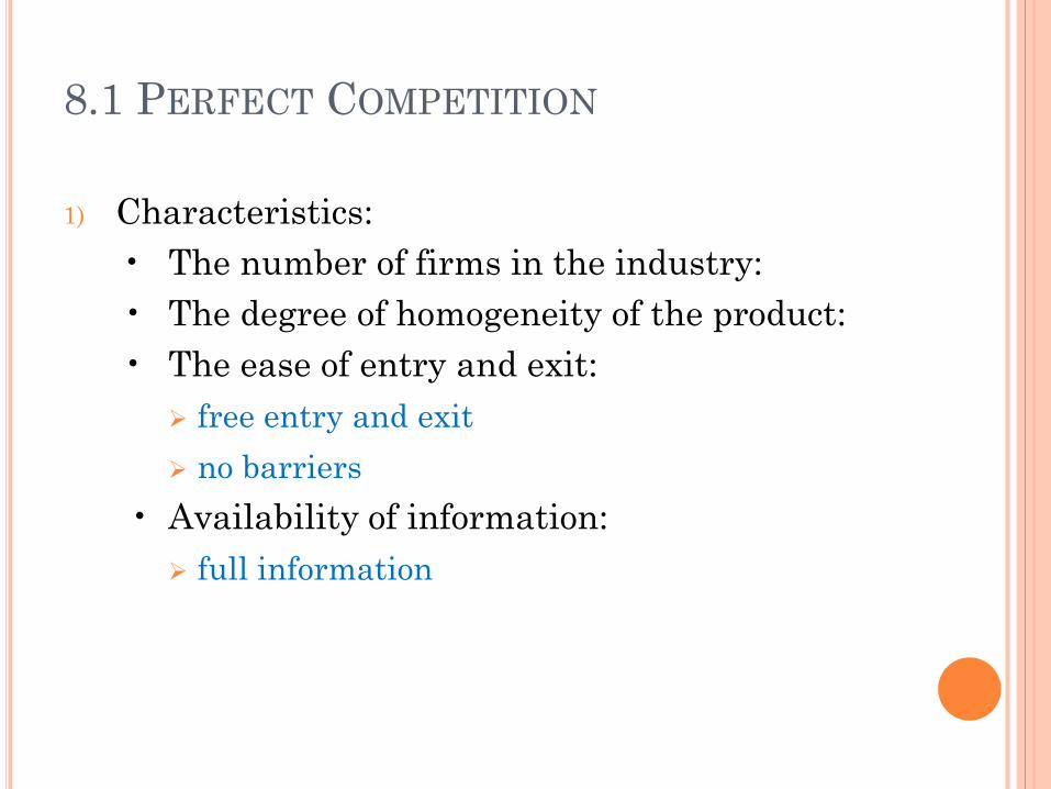
1) Characteristics:• The number of firms in the industry:

a large number of firms each firm is small relative to the market firms are “price takers”

• The degree of homogeneity of the product: homogeneous products no brand perfect substitutes

• The ease of entry and exit: free entry and exit• Availability of information: full information

8.1 PERFECT COMPETITION

1) Characteristics:• The number of firms in the industry:• The degree of homogeneity of the product:• The ease of entry and exit:

free entry and exit no barriers

• Availability of information: full information

8.1 PERFECT COMPETITION

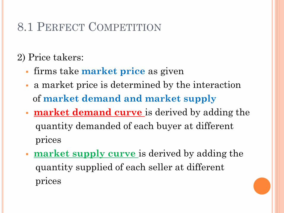
2) Price takers: firms take market price as given a market price is determined by the interaction

of market demand and market supply market demand curve is derived by adding the

quantity demanded of each buyer at different prices

market supply curve is derived by adding the quantity supplied of each seller at different prices

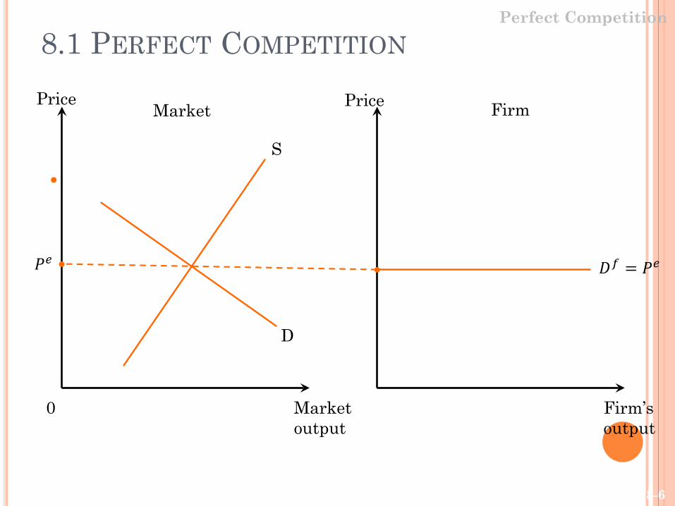
8.1 PERFECT COMPETITIONPerfect Competition

Market output

0

Price

𝑃𝑃𝑒𝑒 𝐷𝐷𝑓𝑓 = 𝑃𝑃𝑒𝑒

D

Price

Firm’soutput

S

Market Firm

8-6

SHORT-RUN PROFIT MAXIMIZATION: REVENUE-COST APPROACH

Perfect Competition

Firm’s output

$

0

Revenue𝑅𝑅 = 𝑃𝑃 × 𝑄𝑄

A

B

Slope of 𝐶𝐶 𝑄𝑄 = 𝑀𝑀𝐶𝐶

E

Costs𝐶𝐶 𝑄𝑄

Slope of 𝑅𝑅 = 𝑀𝑀𝑅𝑅 = 𝑃𝑃

Maximum profits

𝑄𝑄∗

8-7

8.1 PERFECT COMPETITION

3) The Profit maximizing rule Max profit=Total revenue- Total cost Optimal output level (q*)

Marginal Rule: MR(q)=MC(q)

In P.C. MR(q)=P=> P=MC(q)

Optimal output level (q*)

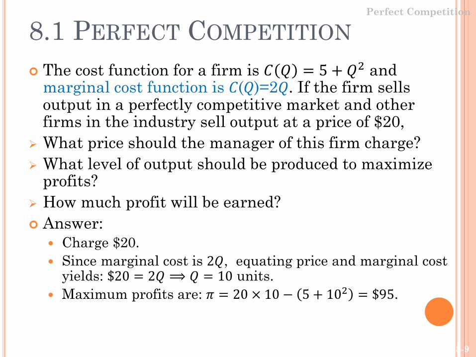
8.1 PERFECT COMPETITION The cost function for a firm is 𝐶𝐶 𝑄𝑄 = 5 + 𝑄𝑄2 and

marginal cost function is 𝐶𝐶(𝑄𝑄)=2𝑄𝑄. If the firm sells output in a perfectly competitive market and other firms in the industry sell output at a price of $20,

What price should the manager of this firm charge? What level of output should be produced to maximize

profits? How much profit will be earned? Answer:

Charge $20. Since marginal cost is 2𝑄𝑄, equating price and marginal cost

yields: $20 = 2𝑄𝑄 ⟹ 𝑄𝑄 = 10 units. Maximum profits are: 𝜋𝜋 = 20 × 10 − 5 + 102 = $95.

Perfect Competition

8-9

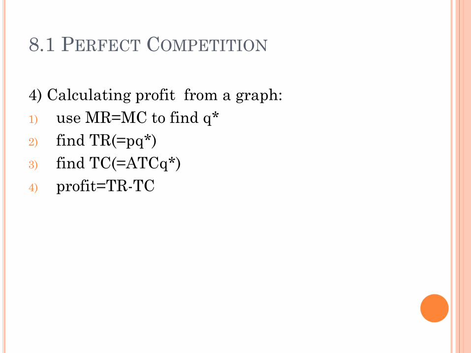
8.1 PERFECT COMPETITION

4) Calculating profit from a graph:1) use MR=MC to find q*2) find TR(=pq*)3) find TC(=ATCq*)4) profit=TR-TC

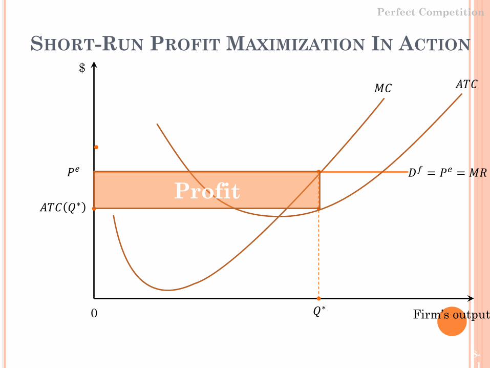
SHORT-RUN PROFIT MAXIMIZATION IN ACTION

Perfect Competition

Firm’s output

$

0 𝑄𝑄∗

𝑃𝑃𝑒𝑒

𝑀𝑀𝐶𝐶 𝐴𝐴𝐴𝐴𝐶𝐶

𝐷𝐷𝑓𝑓 = 𝑃𝑃𝑒𝑒 = 𝑀𝑀𝑅𝑅

𝐴𝐴𝐴𝐴𝐶𝐶 𝑄𝑄∗Profit

8-11

8.1 PERFECT COMPETITION

5) Four scenarios1) P>ATC firm makes a profit2) P=ATC firm breaks even (TR=TC)3) AVC<P<ATC experiences losses but

continues to produce4) P<AVC – shuts down production in the short

run

8.1 PERFECT COMPETITION To maximize short-run profits, a perfectly competitive

firm should produce in the range of increasing marginal cost where 𝑷𝑷 = 𝑴𝑴𝑴𝑴, provided that 𝑷𝑷 ≥ 𝑨𝑨𝑨𝑨𝑴𝑴.

If 𝑷𝑷 < 𝑨𝑨𝑨𝑨𝑴𝑴, the firm should shut down its plant to minimize it losses.

Perfect Competition

8-13

8.1 PERFECT COMPETITION The short-run supply curve for a perfectly competitive firm

is:its marginal cost curve above the minimum point of the 𝑨𝑨𝑨𝑨𝑴𝑴 curve.

Perfect Competition

8-14

8.1 PERFECT COMPETITIONPerfect Competition

Firm’s output

$

0 𝑄𝑄0

𝑃𝑃0

𝑀𝑀𝐶𝐶

𝐴𝐴𝐴𝐴𝐶𝐶𝑃𝑃1

𝑄𝑄1

Short-run supply curve for individual firm

8-15

Perfect Competition

Market outpu

P

0 1

$10

$12

Market supply curve

Individual firm’s supply curve

𝑀𝑀𝐶𝐶𝑖𝑖

500

S

8.1 PERFECT COMPETITION

8-16

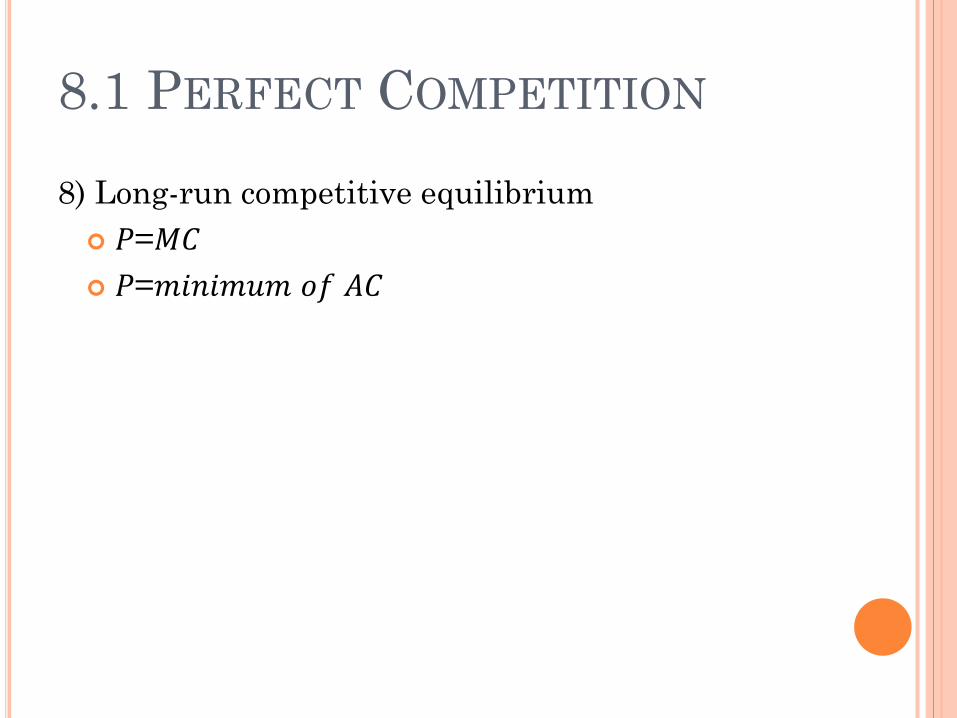
8) Long-run competitive equilibrium 𝑃𝑃=𝑀𝑀𝐶𝐶 𝑃𝑃=𝑚𝑚𝑖𝑖𝑛𝑛𝑖𝑖𝑚𝑚𝑢𝑢𝑚𝑚 𝑜𝑜𝑓𝑓 𝐴𝐴𝐶𝐶

8.1 PERFECT COMPETITION

8.1 LONG-RUN COMPETITIVEEQUILIBRIUM

Perfect Competition

Firm’s output

$

0 𝑄𝑄∗

𝑃𝑃𝑒𝑒

𝑀𝑀𝐶𝐶

𝐴𝐴𝐶𝐶

𝐷𝐷𝑓𝑓 = 𝑃𝑃𝑒𝑒 = 𝑀𝑀𝑅𝑅

Long-run competitive equilibrium

8-18

8.2 MONOPOLY

Definition: A market structure in which a single firm serves an entire market for a good that has no close substitutes.

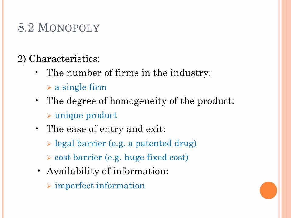
8.2 MONOPOLY

2) Characteristics:• The number of firms in the industry:

a single firm• The degree of homogeneity of the product:

unique product• The ease of entry and exit:

legal barrier (e.g. a patented drug) cost barrier (e.g. huge fixed cost)

• Availability of information: imperfect information

8.2 MONOPOLY

3) Monopolist’s demand and marginal revenue curve: firms are price setters market demand curve is the monopolist’s

demand curveHowever, a monopolist does not have unlimited

market power.

8.2 MONOPOLYMonopoly

Output

Price

0

𝑃𝑃0

𝐷𝐷𝑓𝑓 = 𝐷𝐷𝑀𝑀

𝑃𝑃1

𝑄𝑄1𝑄𝑄0

A

B

Monopolist’s power is constrained by the demand curve.

8-22

8.2 MONOPOLY

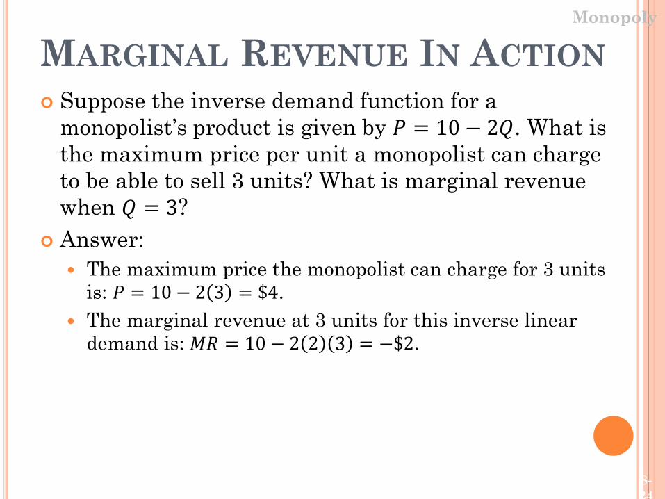
MARGINAL REVENUE IN ACTION Suppose the inverse demand function for a

monopolist’s product is given by 𝑃𝑃 = 10 − 2𝑄𝑄. What is the maximum price per unit a monopolist can charge to be able to sell 3 units? What is marginal revenue when 𝑄𝑄 = 3?

Answer: The maximum price the monopolist can charge for 3 units

is: 𝑃𝑃 = 10 − 2 3 = $4. The marginal revenue at 3 units for this inverse linear

demand is: 𝑀𝑀𝑅𝑅 = 10 − 2 2 3 = −$2.

Monopoly

8-24

8.2 MONOPOLY A profit-maximizing monopolist should produce the

output, 𝑄𝑄𝑀𝑀, such that marginal revenue equals marginal cost:

𝑴𝑴𝑴𝑴 𝑸𝑸𝑴𝑴 = 𝑴𝑴𝑴𝑴 𝑸𝑸𝑴𝑴

Monopoly

8-25

8.2 MONOPOLY

4) Calculating profit from a graph:1) use MR=MC to find q*2) find p (from demand curve)3) find TR(=pq*)4) find TC(=ATCq*)5) profit=TR-TC

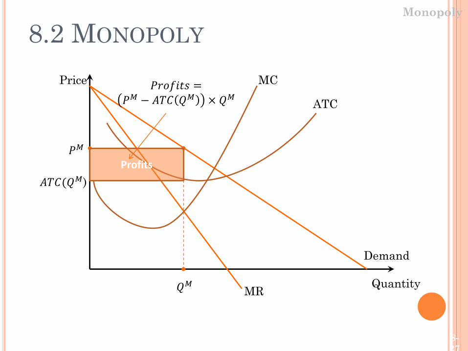
Price

Quantity

Demand

MR

MC

𝑄𝑄𝑀𝑀

𝑃𝑃𝑀𝑀

ATC

𝐴𝐴𝐴𝐴𝐶𝐶(𝑄𝑄𝑀𝑀)Profits

𝑃𝑃𝑃𝑃𝑜𝑜𝑓𝑓𝑖𝑖𝑃𝑃𝑃𝑃 =𝑃𝑃𝑀𝑀 − 𝐴𝐴𝐴𝐴𝐶𝐶 𝑄𝑄𝑀𝑀 × 𝑄𝑄𝑀𝑀

8.2 MONOPOLYMonopoly

8-27

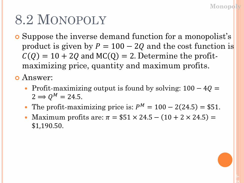
8.2 MONOPOLY Suppose the inverse demand function for a monopolist’s

product is given by 𝑃𝑃 = 100 − 2𝑄𝑄 and the cost function is 𝐶𝐶 𝑄𝑄 = 10 + 2𝑄𝑄 and MC Q = 2. Determine the profit-maximizing price, quantity and maximum profits.

Answer: Profit-maximizing output is found by solving: 100 − 4𝑄𝑄 =

2 ⟹𝑄𝑄𝑀𝑀 = 24.5. The profit-maximizing price is: 𝑃𝑃𝑀𝑀 = 100 − 2 24.5 = $51. Maximum profits are: 𝜋𝜋 = $51 × 24.5− 10 + 2 × 24.5 =

$1,190.50.

Monopoly

8-28

ABSENCE OF A SUPPLY CURVEMonopoly

Recall, firms operating in perfectly competitive markets determine how much output to produce based on price (𝑃𝑃 = 𝑀𝑀𝐶𝐶). Thus, a supply curve exists in perfectly competitive

markets. A monopolist’s market power implies 𝑃𝑃 > 𝑀𝑀𝑅𝑅 = 𝑀𝑀𝐶𝐶.

Thus, there is no supply curve for a monopolist, or in markets served by firms with market power.

8-29

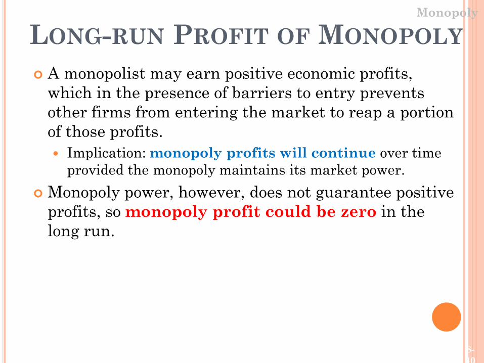
LONG-RUN PROFIT OF MONOPOLY A monopolist may earn positive economic profits,

which in the presence of barriers to entry prevents other firms from entering the market to reap a portion of those profits. Implication: monopoly profits will continue over time

provided the monopoly maintains its market power. Monopoly power, however, does not guarantee positive

profits, so monopoly profit could be zero in the long run.

Monopoly

8-30

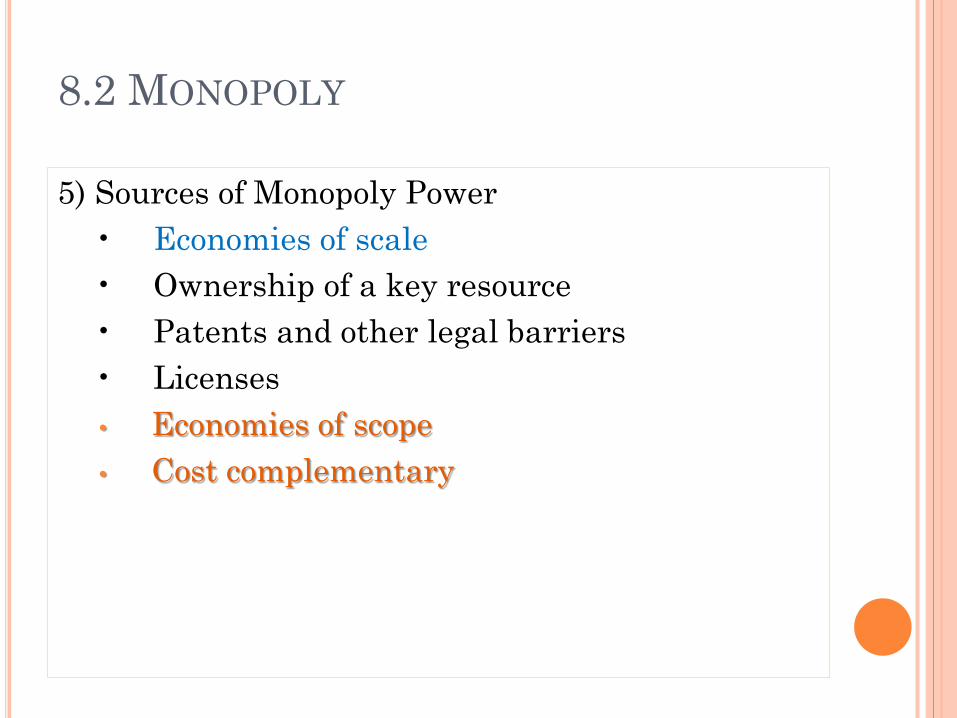
8.2 MONOPOLY

5) Sources of Monopoly Power• Economies of scale• Ownership of a key resource• Patents and other legal barriers • Licenses• Economies of scope• Cost complementary

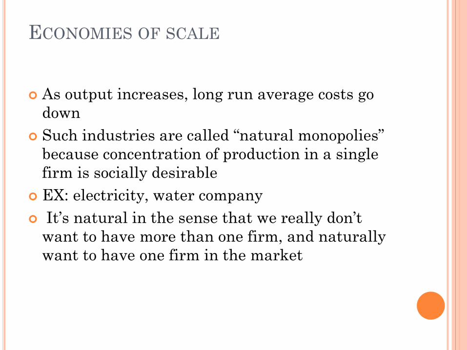
ECONOMIES OF SCALE

As output increases, long run average costs godown

Such industries are called “natural monopolies” because concentration of production in a single firm is socially desirable

EX: electricity, water company It’s natural in the sense that we really don’t

want to have more than one firm, and naturally want to have one firm in the market

8.2 MONOPOLY

5) Source of Monopoly Power• Economies of scale• Ownership of a key resource• Patents and other legal barriers • Licenses•

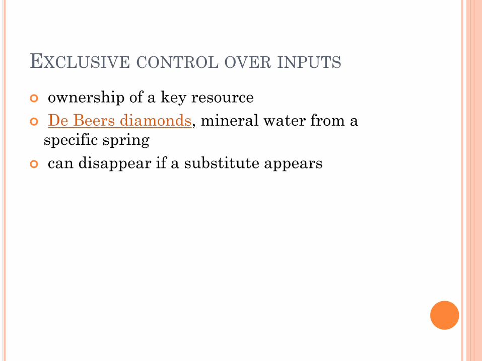
EXCLUSIVE CONTROL OVER INPUTS

ownership of a key resource De Beers diamonds, mineral water from a

specific spring can disappear if a substitute appears

DE BEER

De Beers is well known for its monopoly practices throughout the 20th century, whereby it used its dominant position to manipulate the international diamond market.

8.2 MONOPOLY

5) Source of Mon Economies of scale• Economies of scale• Ownership of a key resource• Patents and other legal barriers • Licenses

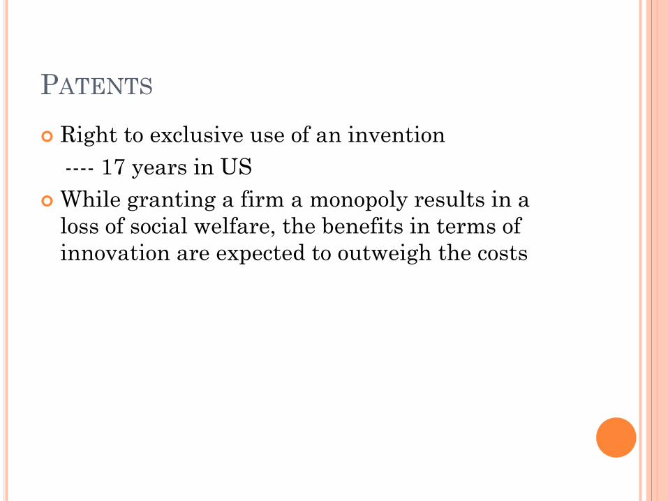
PATENTS

Right to exclusive use of an invention---- 17 years in US

While granting a firm a monopoly results in a loss of social welfare, the benefits in terms of innovation are expected to outweigh the costs

8.2 MONOPOLY

5) Source of Mon Economies of scale• Economies of scale• Ownership of a key resource• Patents and other legal barriers • Licenses

LICENSES

Authorities give permission to one firm to operate EX: airport vendors; exclusive rights to sell on

campus PP245

LONG-RUN PROFIT OF MONOPOLY A monopolist may earn positive economic profits,

which in the presence of barriers to entry prevents other firms from entering the market to reap a portion of those profits. Implication: monopoly profits will continue over time

provided the monopoly maintains its market power. Monopoly power, however, does not guarantee positive

profits, so monopoly profit could be zero in the long run.

Monopoly

8-40

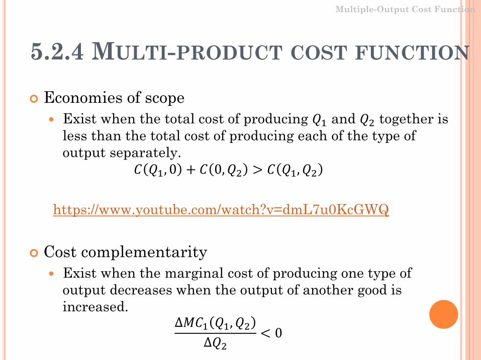
5.2.4 MULTI-PRODUCT COST FUNCTION

Economies of scope Exist when the total cost of producing 𝑄𝑄1 and 𝑄𝑄2 together is

less than the total cost of producing each of the type of output separately.

𝐶𝐶 𝑄𝑄1, 0 + 𝐶𝐶 0,𝑄𝑄2 > 𝐶𝐶 𝑄𝑄1,𝑄𝑄2

https://www.youtube.com/watch?v=dmL7u0KcGWQ

Cost complementarity Exist when the marginal cost of producing one type of

output decreases when the output of another good is increased.

∆𝑀𝑀𝐶𝐶1 𝑄𝑄1,𝑄𝑄2∆𝑄𝑄2

< 0

Multiple-Output Cost Function

5-41

MULTIPLANT DECISIONS Often a monopolist produces output in different

locations. Implications: manager has to determine how much output

to produce at each plant. Consider a monopolist producing output at two plants:

The cost of producing 𝑄𝑄1 units at plant 1 is 𝐶𝐶 𝑄𝑄1 , and the cost of producing 𝑄𝑄2 at plant 2 is 𝐶𝐶 𝑄𝑄2 .

When the monopolist produces a homogeneous product, the per-unit price consumers are willing to pay for the total output produced at the two plants is 𝑃𝑃 𝑄𝑄 , where 𝑄𝑄 = 𝑄𝑄1 +𝑄𝑄2.

Monopoly

8-42

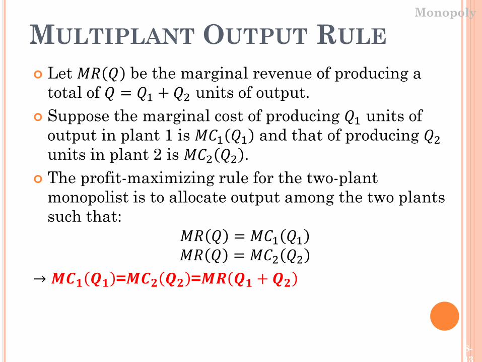
MULTIPLANT OUTPUT RULE Let 𝑀𝑀𝑅𝑅 𝑄𝑄 be the marginal revenue of producing a

total of 𝑄𝑄 = 𝑄𝑄1 + 𝑄𝑄2 units of output. Suppose the marginal cost of producing 𝑄𝑄1 units of

output in plant 1 is 𝑀𝑀𝐶𝐶1 𝑄𝑄1 and that of producing 𝑄𝑄2units in plant 2 is 𝑀𝑀𝐶𝐶2 𝑄𝑄2 .

The profit-maximizing rule for the two-plant monopolist is to allocate output among the two plants such that:

𝑀𝑀𝑅𝑅 𝑄𝑄 = 𝑀𝑀𝐶𝐶1 𝑄𝑄1𝑀𝑀𝑅𝑅 𝑄𝑄 = 𝑀𝑀𝐶𝐶2 𝑄𝑄2

→ 𝑴𝑴𝑴𝑴𝟏𝟏 𝑸𝑸𝟏𝟏 =𝑴𝑴𝑴𝑴𝟐𝟐 𝑸𝑸𝟐𝟐 =𝑴𝑴𝑴𝑴 𝑸𝑸𝟏𝟏 + 𝑸𝑸𝟐𝟐

Monopoly

8-43

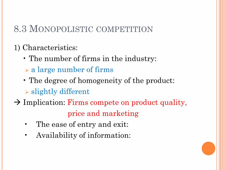
8.3 MONOPOLISTIC COMPETITION

1) Characteristics:• The number of firms in the industry: a large number of firms

• The degree of homogeneity of the product: slightly different

Implication: Firms compete on product quality, price and marketing

• The ease of entry and exit:• Availability of information:

8.3 MONOPOLISTIC COMPETITION

1) Characteristics:• The number of firms in the industry:• The degree of homogeneity of the product:

Implication: Firms compete on product quality, price and marketing

• The ease of entry and exit: free to enter and exit the industry

Implication: In the long run equilibrium, firm’s profit is zero

• Availability of information: imperfect information

PHONE INDUSTRY

WOMEN’S HANDBAG INDUSTRY

8.3 MONOPOLISTIC COMPETITION

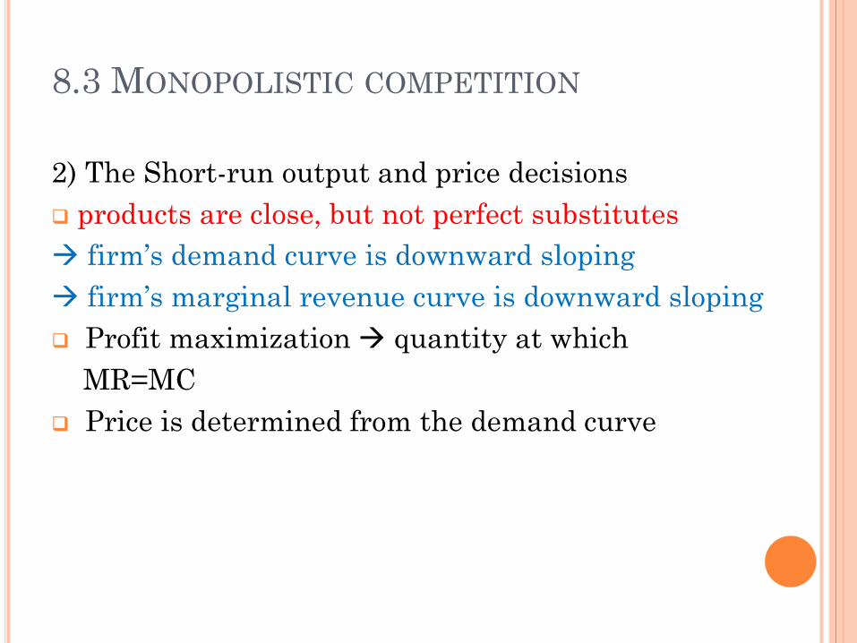
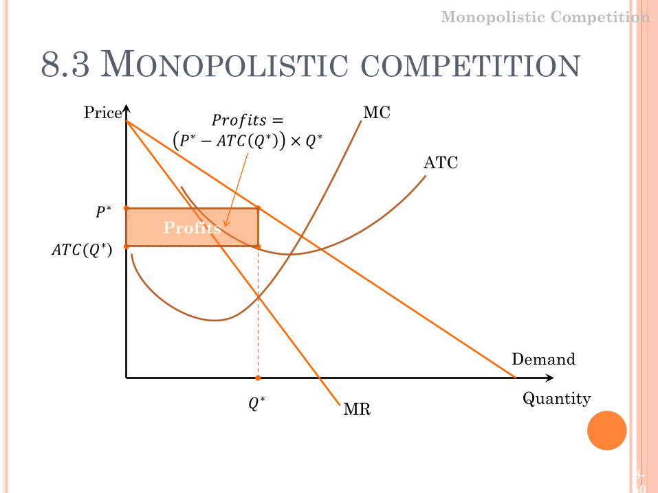
2) The Short-run output and price decisions products are close, but not perfect substitutes firm’s demand curve is downward sloping firm’s marginal revenue curve is downward sloping Profit maximization quantity at which

MR=MC Price is determined from the demand curve

8.3 MONOPOLISTIC COMPETITION

3) The Long-run equilibrium If firms in monopolistically competitive markets earn short-run profits, additional firms will enter in the long run

to capture some of those profits. losses, some firms will exit the industry in the

long run.

Price

Quantity

Demand

MR

MC

𝑄𝑄∗

𝑃𝑃∗

ATC

8.3 MONOPOLISTIC COMPETITION

Monopolistic Competition

𝐴𝐴𝐴𝐴𝐶𝐶(𝑄𝑄∗)

𝑃𝑃𝑃𝑃𝑜𝑜𝑓𝑓𝑖𝑖𝑃𝑃𝑃𝑃 =𝑃𝑃∗ − 𝐴𝐴𝐴𝐴𝐶𝐶 𝑄𝑄∗ × 𝑄𝑄∗

Profits

8-50

Price

Quantity of Brand X

Demand0

MR0

MC

𝑄𝑄∗

𝑃𝑃∗

ATC

8.3 MONOPOLISTIC COMPETITIONMonopolistic Competition

Demand1

MR1

Due to entry of new firms selling other brands

8-51

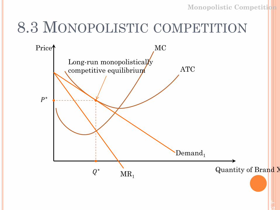
Price

Quantity of Brand X

MC

𝑄𝑄∗

𝑃𝑃∗

ATC

8.3 MONOPOLISTIC COMPETITION

Monopolistic Competition

Demand1

MR1

Long-run monopolistically competitive equilibrium

8-52

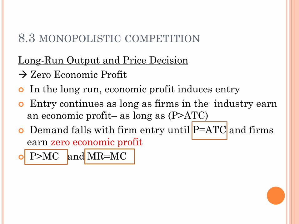
8.3 MONOPOLISTIC COMPETITION

Long-Run Output and Price Decision Zero Economic Profit In the long run, economic profit induces entry Entry continues as long as firms in the industry earn

an economic profit– as long as (P>ATC) Demand falls with firm entry until P=ATC and firms

earn zero economic profit P>MC and MR=MC

8.3 MONOPOLISTIC COMPETITION In the long run, monopolistically competitive firms

produce a level of output such that: 𝑃𝑃 > 𝑀𝑀𝐶𝐶 markup 𝑃𝑃 = 𝐴𝐴𝐴𝐴𝐶𝐶 > 𝑚𝑚𝑖𝑖𝑛𝑛𝑖𝑖𝑚𝑚𝑢𝑢𝑚𝑚 𝑜𝑜𝑓𝑓 𝑎𝑎𝑎𝑎𝑎𝑎𝑃𝑃𝑎𝑎𝑎𝑎𝑎𝑎 𝑐𝑐𝑜𝑜𝑃𝑃𝑃𝑃𝑃𝑃 excess capacity

Monopolistic Competition

8-54

MONOPOLY VS. PERFECT COMPETITION

Monopoly: Higher price Lower quantity Lower consumer surplus Higher producer surplus Lower total surplus Dead weight loss exists

CONCLUSION Firms operating in a perfectly competitive market

take the market price as given. Produce output where 𝑃𝑃 = 𝑀𝑀𝐶𝐶. Firms may earn profits or losses in the short run. but, in the long run, entry or exit forces economic profits to

zero. A monopoly firm, in contrast, can earn persistent

profits provided that the source of monopoly power is not eliminated.

A monopolistically competitive firm can earn profits in the short run, but entry by competing brands will erode these profits in the long run.

8-56