chapter 8: fundamentals of capital budgeting

Chapter 8: Fundamentals of Capital Budgeting - 1

Supplement to Text

Chapter 8: Fundamentals of Capital Budgeting

Note: Read the chapter then look at the following.

Fundamental question: How do we determine the cash flows we need to calculate the net present

value of a project?

Key: most managers estimate a project’s cash flows in two steps:

1) Impact of the project on the firm’s incremental earnings

2) Use incremental earnings to determine the project’s incremental cash flows

Notes:

1) incremental = change as a result of the investment decision

2) revenues and expenses occur throughout the year, but we will treat them as if they

come at end of the year

=> this is a standard assumption used by the text

8.1 Forecasting Earnings

Basic Question: How do firm’s unlevered earnings change as result of an investment

decision?

A. Excel

=> for real projects, difficult to do by hand => use Excel

Note: don’t hardcode (enter numbers) directly into formulas. Have your formulas refer to

the section of your spreadsheet where you input the numbers (the text makes this

point on p. 245).


Supplement to Text

B. Calculating by hand:

𝑈𝑁𝐼 = 𝐸𝐵𝐼𝑇 × (1 − 𝜏𝑐) = (𝑅 − 𝐸 − 𝐷)(1 − 𝜏𝑐) (8.2)

where:

UNI = incremental unlevered net income

=> counting only incremental operating cash flows, but no financing cash flows

EBIT = incremental earnings before interest and taxes

c = firm’s marginal corporate tax rate

R = incremental revenues

E = incremental expenses (or costs)

Note: Book uses costs, I will use “expenses” so can have an “E” instead of a “C”

in the equation. Will use “C” for cash in new working capital in section 8.2

D = incremental depreciation

C. Identifying Incremental Earnings

1. General Principles

Basic question: How do the earnings (and cash flows) for the entire firm differ with

the project verses without the project?

=> count anything that changes for the firm

=> count nothing that remains the same

Example of costs that often don’t change with new project: fixed overhead

expenses

=> don’t count previous or committed spending unless can get some back if don’t

proceed

=> part can’t get back is called sunk costs

Ex. money already spent to research and develop a product

Ex. completed feasibility studies

Ex. money spent on a partially completed building that can be sold


Supplement to Text

2. Specific Issues

a. Revenues and Costs

=> count changes in revenues or expenses that result from the project

=> count changes in revenues or expenses elsewhere in the firm if it undertakes

the project

=> called project externalities or cannibalization

Ex. sales from new project replace existing sales

Ex. no longer paying overtime at an existing facility

=> don’t count any interest expense

=> accepting/rejecting the project is a separate decision from how the firm

will finance the project

=> taxes are an expense

=> relevant tax rate: firm’s marginal corporate tax rate

b. Fixed assets

1) Fixed assets that acquire because undertake project

a) cash outflow when pay to build or acquire

b) reduction in taxes because of depreciation in years after the acquisition

=> treat as a cash inflow since reduces outflow for tax payments

Note: depreciation does not directly impact cash flow but indirectly

through taxes

=> can use straight line or accelerated (MACRS) depreciation

Note: firms often use a different depreciation method for taxes and

accounting statements

=> use depreciation expense calculated for taxes (because of tax

effect on cash flows).


Supplement to Text

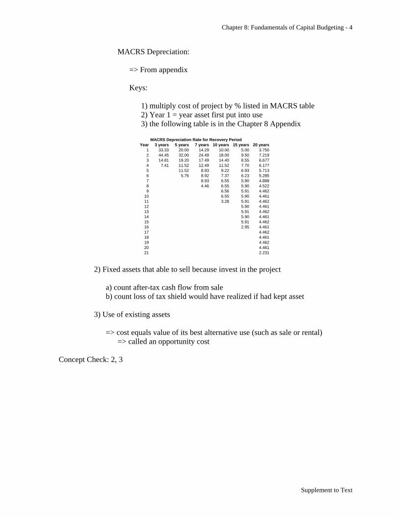
MACRS Depreciation:

=> From appendix

Keys:

1) multiply cost of project by % listed in MACRS table

2) Year 1 = year asset first put into use

3) the following table is in the Chapter 8 Appendix

2) Fixed assets that able to sell because invest in the project

a) count after-tax cash flow from sale

b) count loss of tax shield would have realized if had kept asset

3) Use of existing assets

=> cost equals value of its best alternative use (such as sale or rental)

=> called an opportunity cost

Concept Check: 2, 3

MACRS Depreciation Rate for Recovery Period

Year 3 years 5 years 7 years 10 years 15 years 20 years

1 33.33 20.00 14.29 10.00 5.00 3.750

2 44.45 32.00 24.49 18.00 9.50 7.219

3 14.81 19.20 17.49 14.40 8.55 6.677

4 7.41 11.52 12.49 11.52 7.70 6.177

5 11.52 8.93 9.22 6.93 5.713

6 5.76 8.92 7.37 6.23 5.285

7 8.93 6.55 5.90 4.888

8 4.46 6.55 5.90 4.522

9 6.56 5.91 4.462

10 6.55 5.90 4.461

11 3.28 5.91 4.462

12 5.90 4.461

13 5.91 4.462

14 5.90 4.461

15 5.91 4.462

16 2.95 4.461

17 4.462

18 4.461

19 4.462

20 4.461

21 2.231


Supplement to Text

8.2 Determining Free Cash Flow and NPV

A. Calculating Free Cash Flow from Earnings

Keys:

1) start with incremental unlevered net income

2) back out non-cash items in UNI

3) add cash items not in UNI

FCF = UNI + D – CE - NWC (8.5a)

where:

CE = incremental after-tax capital expenditures

NWC = change in net working capital associated with project

NWCt = NWCt – NWCt-1 (8.4)

NWC = CA – CL = C + AR + I – AP (8.3)

CA = incremental current assets

CL = incremental current liabilities

C = incremental cash

AR = incremental accounts receivable

I = incremental inventory

AP = incremental accounts payable

𝐹𝐶𝐹 = (𝑅 − 𝐸 − 𝐷) × (1 − 𝜏𝑐) + 𝐷 − 𝐶𝐸 − ∆𝑁𝑊𝐶 (8.5b)

𝐹𝐶𝐹 = (𝑅 − 𝐸) × (1 − 𝜏𝑐) − 𝐶𝐸 − ∆𝑁𝑊𝐶 + 𝜏𝑐 × 𝐷 (8.6)

Note: 𝜏𝑐 × 𝐷 is the depreciation tax shield

=> reduction in taxes that stem from deducting deprecation for tax purposes

=> depreciation increases cash flows because reduce tax payments

B. Notes

1. Depreciation (D)

=> add back to FCF since subtracted from UNI but doesn’t involve a cash outlay


Supplement to Text

2. Capital Expenditures (CE)

=> incremental capital spending creates an outflow of cash that isn’t counted in UNI

Note: cost is recognized in UNI over the life of the asset through depreciation

=> incremental asset sales are entered as a negative CE

=> creates a cash inflow

=> positive impact through equations as subtract a negative CE

=> must also consider tax implications of any asset sales

3. Change in Net Working Capital (NWC)

1) sales on credit generate revenue but no cash flow

2) the collection of receivables generates a cash inflow but no revenue

3) the sale of inventory generates an expense but no cash outflow

4) the purchase of inventory generates a cash outflow but no expense

=> subtracting the change in net working capital adjusts for these issues

Notes on changes in net working capital:

1. recovery of net working capital

=> Changes in net working capital are usually reversed at the end of the

project

Ex. Cash put into cash registers is no longer needed when close a store

2. taxability

=> changes in net working capital are not taxable

=> buying inventory doesn’t create taxable income, selling inventory for a

profit does

D. Calculating NPV

𝑃𝑉(𝐹𝐶𝐹𝑡) =𝐹𝐶𝐹𝑡

(1+𝑟)𝑡 = 𝐹𝐶𝐹𝑡 ×1

(1+𝑟)𝑡 (8.7)

Note: We really don’t need this equation. It is essentially (4.2)


Supplement to Text

8.3 Choosing Among Alternatives

A. Evaluating Manufacturing Alternatives

Note: To decide between alternatives, can compare the NPVs of alternatives.

However, can also decide by calculating the NPV of the difference in cash flows.

Example from text (p. 247):

Differences in Cash Flows (In-House – Outsourced):

Yr 0 = –3000 = – 3000 – 0

Yr 1 = –117 = – 5067 – (– 4950)

Yr 2 – 4 = +900 = – 5700 – (– 6600)

Yr 5 = +1017 = – 633 – (– 1650)

NPV (differences) = −3000 −117

1.12+

900

.12(1 − (

1

1.12)

3

) (1

1.12) +

1017

(1.12)5 = −597

Note: Same result as text

Difference in text = – 20,107 – (– 19,510) = – 597

Video Solution

Concept Check: all

8.4 Further Adjustments to Free Cash Flow

1. Other non-cash items

=> should back out (from UNI) any other non-cash items

2. Timing of Cash Flows

=> cash flows likely spread throughout year instead of at end of year

=> might increase accuracy if estimate cash flows over smaller time periods

3. Accelerated Depreciation

Key issue: accelerated depreciation allows earlier recognition of depreciation

=> get cash flows from tax shield earlier

=> present value of tax shield higher

http://business.baylor.edu/steve_rich/fin3310/videos/Ch08-3EX.mov


Supplement to Text

Note on Example 8.5: Firms can start depreciating the asset as soon as it is put into use.

Unless stated otherwise, I will assume that if we build or acquire an asset today, it

will be put into use at some point during the first year and so recognize depreciation

for the first time in year 1.

4. Liquidation or Salvage Value

G = SP – BV (8.8)

where:

G = gain

SP = sales price

BV = book value

BV = PP – AD (8.9)

where:

PP = purchase price

AD = accumulated depreciation

ATCF = SP – c × G (8.10)

where:

ATCF = after-tax cash flow from asset sale

5. Terminal or Continuation Value

Key issue: often assume cash flows grow at some constant rate forever beyond horizon

over which forecast cash flows.

6. Tax Carryforwards and Carrybacks

Key issue: can carryback losses to offset profits for previous two years and/or can

carryforward losses to offset profits for following 20 years.

A. Examples

Note: In the following examples, we start with the simplest case in which free cash flow

equals unlevered net income. Each subsequent example builds on the previous

example by adding (or changing) an assumption. The new assump are underlined in

each example.


Supplement to Text

Example 1:

Assume you are trying to decide whether to rent a building for $30,000 a year for the

next 2 years (payments are due at the end of the year). A year from today you plan

to purchase inventory for $50,000 that you will sell immediately for $110,000.

Two years from today you plan to purchase inventory for $70,000 that you will

sell immediately for $150,000. Calculate the store’s incremental unlevered net

income and free cash flow for each year of operation if the corporate tax rate is

35%.

𝑈𝑁𝐼 = 𝐸𝐵𝐼𝑇 × (1 − 𝜏𝑐) = (𝑅 − 𝐸 − 𝐷)(1 − 𝜏𝑐)

NWC = C + AR + I – AP FCF = UNI + D – CE - NWC

UNI1 = (110,000 – (30,000+50,000) – 0)(1 – .35) = $19,500

UNI2 = (150,000 – (30,000+70,000) – 0)(1 – .35) = $32,500

FCF1 = 19,500

FCF2 = 32,500

Video Solution

Notes:

1) FCF = UNI since no depreciation, capital expenditures or changes in net

working capital

2) Will build on this example. New information in later examples will be

underlined.

http://business.baylor.edu/steve_rich/fin3310/videos/Ch08-4A1EX.mov


Supplement to Text

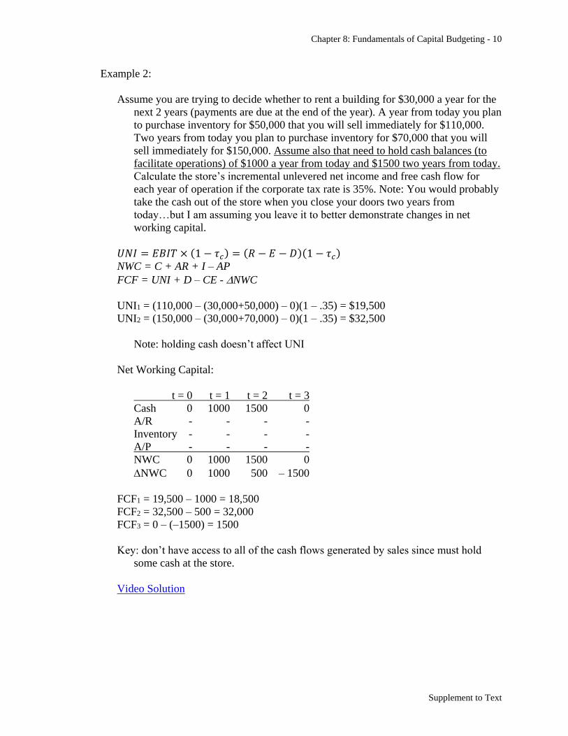
Example 2:





sell immediately for $150,000. Assume also that need to hold cash balances (to

facilitate operations) of $1000 a year from today and $1500 two years from today.

Calculate the store’s incremental unlevered net income and free cash flow for

each year of operation if the corporate tax rate is 35%. Note: You would probably

take the cash out of the store when you close your doors two years from

today…but I am assuming you leave it to better demonstrate changes in net

working capital.

𝑈𝑁𝐼 = 𝐸𝐵𝐼𝑇 × (1 − 𝜏𝑐) = (𝑅 − 𝐸 − 𝐷)(1 − 𝜏𝑐)


UNI1 = (110,000 – (30,000+50,000) – 0)(1 – .35) = $19,500

UNI2 = (150,000 – (30,000+70,000) – 0)(1 – .35) = $32,500

Note: holding cash doesn’t affect UNI

Net Working Capital:

t = 0 t = 1 t = 2 t = 3

Cash 0 1000 1500 0

A/R - - - -

Inventory - - - -

A/P - - - -

NWC 0 1000 1500 0

NWC 0 1000 500 – 1500

FCF1 = 19,500 – 1000 = 18,500

FCF2 = 32,500 – 500 = 32,000

FCF3 = 0 – (–1500) = 1500

Key: don’t have access to all of the cash flows generated by sales since must hold

some cash at the store.

Video Solution



Supplement to Text

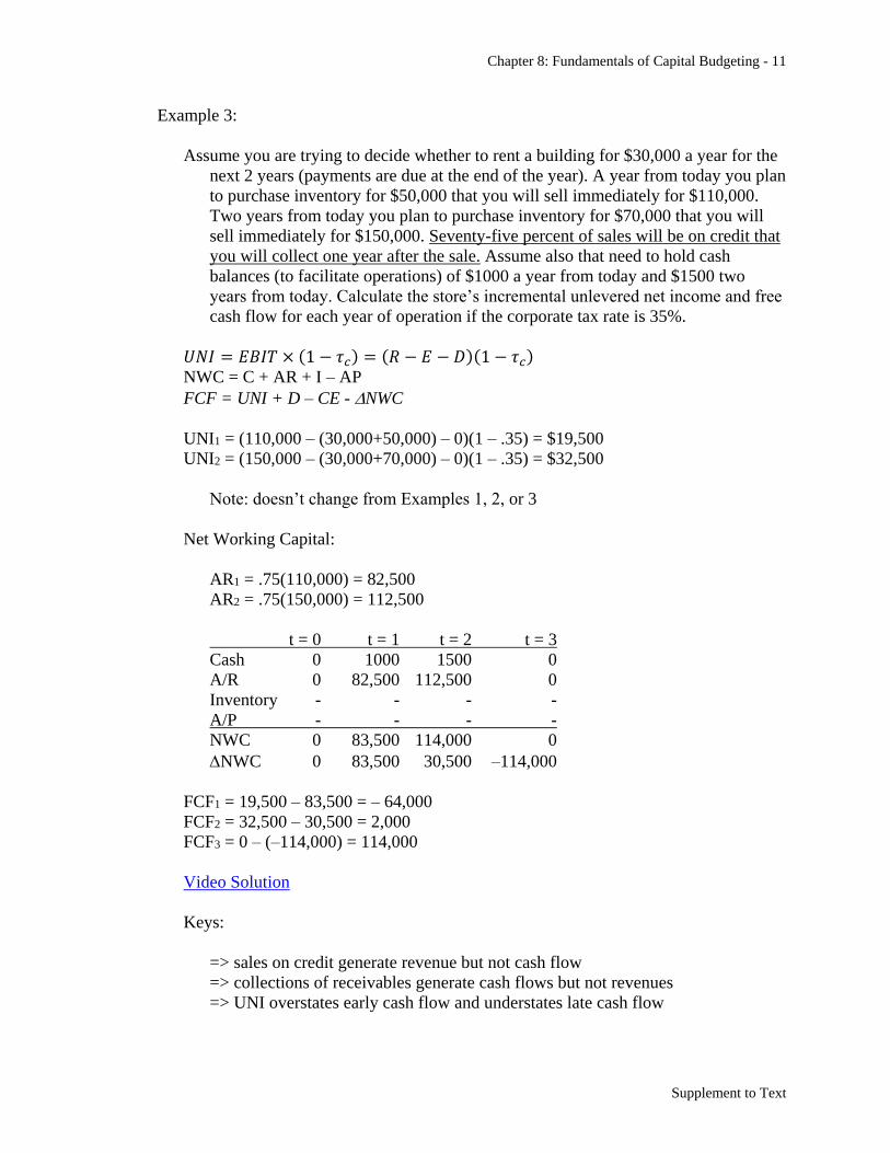
Example 3:





sell immediately for $150,000. Seventy-five percent of sales will be on credit that

you will collect one year after the sale. Assume also that need to hold cash

balances (to facilitate operations) of $1000 a year from today and $1500 two

years from today. Calculate the store’s incremental unlevered net income and free

cash flow for each year of operation if the corporate tax rate is 35%.

𝑈𝑁𝐼 = 𝐸𝐵𝐼𝑇 × (1 − 𝜏𝑐) = (𝑅 − 𝐸 − 𝐷)(1 − 𝜏𝑐)


UNI1 = (110,000 – (30,000+50,000) – 0)(1 – .35) = $19,500

UNI2 = (150,000 – (30,000+70,000) – 0)(1 – .35) = $32,500

Note: doesn’t change from Examples 1, 2, or 3


AR1 = .75(110,000) = 82,500

AR2 = .75(150,000) = 112,500

t = 0 t = 1 t = 2 t = 3

Cash 0 1000 1500 0

A/R 0 82,500 112,500 0

Inventory - - - -

A/P - - - -

NWC 0 83,500 114,000 0

NWC 0 83,500 30,500 –114,000

FCF1 = 19,500 – 83,500 = – 64,000

FCF2 = 32,500 – 30,500 = 2,000

FCF3 = 0 – (–114,000) = 114,000

Video Solution

Keys:

=> sales on credit generate revenue but not cash flow

=> collections of receivables generate cash flows but not revenues

=> UNI overstates early cash flow and understates late cash flow



Supplement to Text

Example 4:


next 2 years (payments are due at the end of the year). Today you plan to

purchase inventory for $50,000 that you will sell a year from today for $110,000.

A year from today you plan to purchase inventory for $70,000 that you will sell

two years from today for $150,000. Sixty percent of all inventory purchases will

be on credit due one year after you buy it. Seventy-five percent of sales will be on

credit that you will collect one year after the sale. Assume also that need to hold

cash balances (to facilitate operations) of $1000 a year from today and $1500 two

years from today. Calculate the store’s incremental unlevered net income and free

cash flow for each year of operation if the corporate tax rate is 35%.

𝑈𝑁𝐼 = 𝐸𝐵𝐼𝑇 × (1 − 𝜏𝑐) = (𝑅 − 𝐸 − 𝐷)(1 − 𝜏𝑐)


UNI1 = (110,000 – (30,000+50,000) – 0)(1 – .35) = $19,500

UNI2 = (150,000 – (30,000+70,000) – 0)(1 – .35) = $32,500

Note: doesn’t change from previous examples


AP0 = .6(50,000) = 30,000

AP1 = .6(70,000) = 42,000

t = 0 t = 1 t = 2 t = 3

Cash 0 1000 1500 0

A/R 0 82,500 112,500 0

Inventory 50,000 70,000 0 0

A/P 30,000 42,000 0 0

NWC 20,000 111,500 114,000 0

NWC 20,000 91,500 2500 –114,000

FCF0 = 0 – 20,000 = – 20,000

FCF1 = 19,500 – 91,500 = – 72,000

FCF2 = 32,500 – 2,500 = 30,000

FCF3 = 0 – (–114,000) = 114,000

Video Solution

Keys:

=> purchases on credit offset to some extent the differences between UNI and

Cash Flow associated with buying inventory



Supplement to Text

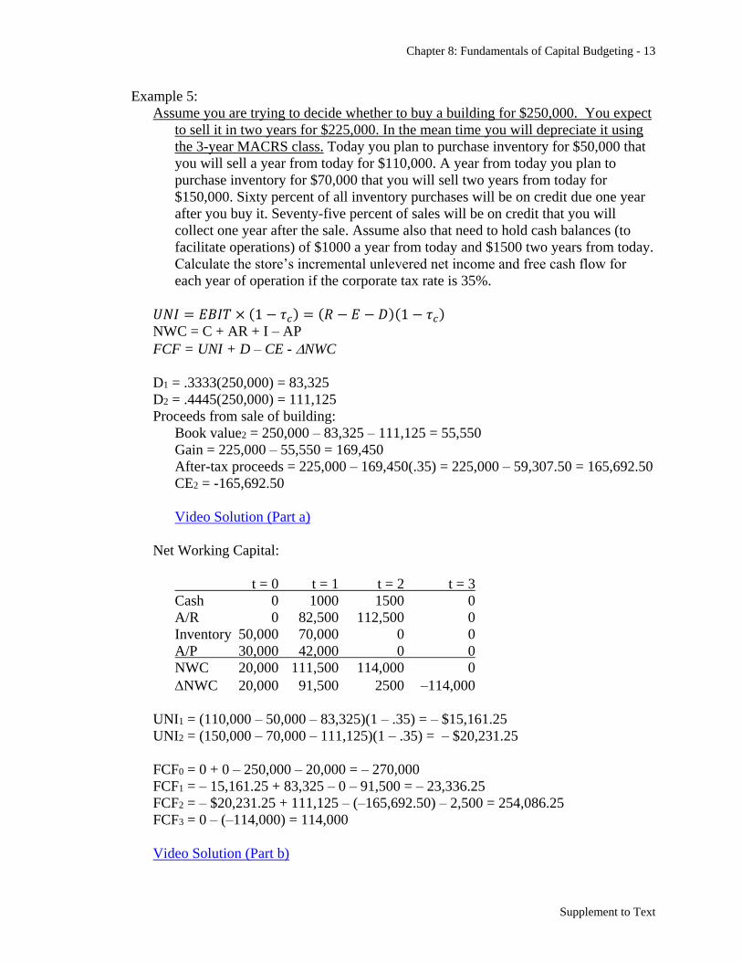
Example 5:

Assume you are trying to decide whether to buy a building for $250,000. You expect

to sell it in two years for $225,000. In the mean time you will depreciate it using

the 3-year MACRS class. Today you plan to purchase inventory for $50,000 that

you will sell a year from today for $110,000. A year from today you plan to

purchase inventory for $70,000 that you will sell two years from today for

$150,000. Sixty percent of all inventory purchases will be on credit due one year

after you buy it. Seventy-five percent of sales will be on credit that you will

collect one year after the sale. Assume also that need to hold cash balances (to

facilitate operations) of $1000 a year from today and $1500 two years from today.

Calculate the store’s incremental unlevered net income and free cash flow for

each year of operation if the corporate tax rate is 35%.

𝑈𝑁𝐼 = 𝐸𝐵𝐼𝑇 × (1 − 𝜏𝑐) = (𝑅 − 𝐸 − 𝐷)(1 − 𝜏𝑐)


D1 = .3333(250,000) = 83,325

D2 = .4445(250,000) = 111,125

Proceeds from sale of building:

Book value2 = 250,000 – 83,325 – 111,125 = 55,550

Gain = 225,000 – 55,550 = 169,450

After-tax proceeds = 225,000 – 169,450(.35) = 225,000 – 59,307.50 = 165,692.50

CE2 = -165,692.50

Video Solution (Part a)


t = 0 t = 1 t = 2 t = 3

Cash 0 1000 1500 0

A/R 0 82,500 112,500 0

Inventory 50,000 70,000 0 0

A/P 30,000 42,000 0 0

NWC 20,000 111,500 114,000 0

NWC 20,000 91,500 2500 –114,000

UNI1 = (110,000 – 50,000 – 83,325)(1 – .35) = – $15,161.25

UNI2 = (150,000 – 70,000 – 111,125)(1 – .35) = – $20,231.25

FCF0 = 0 + 0 – 250,000 – 20,000 = – 270,000

FCF1 = – 15,161.25 + 83,325 – 0 – 91,500 = – 23,336.25

FCF2 = – $20,231.25 + 111,125 – (–165,692.50) – 2,500 = 254,086.25

FCF3 = 0 – (–114,000) = 114,000

Video Solution (Part b)

http://business.baylor.edu/steve_rich/fin3310/videos/Ch08-4A5EXa.mov

http://business.baylor.edu/steve_rich/fin3310/videos/Ch08-4A5EXb.mov


Supplement to Text

Concept Check: all

8.5 Analyzing the Project

Key to all of section 8.5: Using goal seek and data tables in Excel.

Break-even: level of one input variable that makes NPV = 0

Sensitivity analysis: examines impact on NPV of changing one input variable

Key concern: identify which worse-case assumptions lead to a negative NPV

Scenario analysis: examines impact on NPV of changing multiple related input variables

Concept Check: all

Chapter 8 Appendix: MACRS Depreciation

=> covered earlier in notes

chapter 8: fundamentals of capital budgeting

Documents