chapter 8 fractal properties of plants - algorithmic...

$: Chapter 8 Fractal properties of plants - Algorithmic Botanyalgorithmicbotany.org/papers/abop/abop-ch8.pdf · Chapter 8 Fractal properties of plants What is a fractal? In his 1982$
Chapter 8

Fractal properties of plants

What is a fractal? In his 1982 book, Mandelbrot defines it as a set with Fractals vs.finite curvesHausdorff-Besicovitch dimension DH strictly exceeding the topological

dimension DT [95, page 15]. In this sense, none of the figures presentedin this book are fractals, since they all consist of a finite number ofprimitives (lines or polygons), and DH = DT . However, the situationchanges dramatically if the term “fractal” is used in a broader sense [95,page 39]:

Strictly speaking, the triangle, the Star of David, and thefinite Koch teragons are of dimension 1. However, bothintuitively and from the pragmatic point of view of the sim-plicity and naturalness of the corrective terms required, it isreasonable to consider an advanced Koch teragon as beingcloser to a curve of dimension log 4/log 3 than to a curveof dimension 1.

Thus, a finite curve can be considered an approximate renderingof an infinite fractal as long as the interesting properties of both areclosely related. In the case of plant models, this distinctive feature isself-similarity.

The use of approximate figures to illustrate abstract concepts has a Fractals vs.plantslong tradition in geometry. After all, even the primitives of Euclidean

geometry — a point and a line — cannot be drawn exactly. An in-teresting question, however, concerns the relationship between fractalsand real biological structures. The latter consist of a finite number ofcells, thus are not fractals in the strict sense of the word. To considerreal plants as approximations of “perfect” fractal structures would beacceptable only if we assumed Plato’s view of the supremacy of ideasover their mundane realization. A viable approach is the opposite one,to consider fractals as abstract descriptions of the real structures. Atfirst sight, this concept may seem strange. What can be gained by Complexity of

fractalsreducing an irregular contour of a compound leaf to an even more ir-regular fractal? Would it not be simpler to characterize the leaf using

176 Chapter 8. Fractal properties of plants

a smooth curve? The key to the answer lies in the meaning of the term“simple.” A smooth curve may seem intuitively simpler than a fractal,but as a matter of fact, the reverse is often true [95, page 41]. Accord-ing to Kolmogorov [80], the complexity of an object can be measuredby the length of the shortest algorithm that generates it. In this sense,many fractals are particularly simple objects.

The above discussion of the relationship between fractals and plantsPreviousviewpoints did not emerge in a vacuum. Mandelbrot [95] gives examples of the re-

cursive branching structures of trees and flowers, analyzes theirHausdorff-Besicovitch dimension and writes inconclusively “trees maybe called fractals in part.” Smith [136] recognizes similarities betweenalgorithms yielding Koch curves and branching plant-like structures,but does not qualify plant models as fractals. These structures are pro-duced in a finite number of steps and consist of a finite number of linesegments, while the “notion of fractal is defined only in the limit.” Op-penheimer [105] uses the term “fractal” more freely, exchanging it withself-similarity, and comments: “The geometric notion of self-similaritybecame a paradigm for structure in the natural world. Nowhere is thisprinciple more evident than in the world of botany.” The approach pre-sented in this chapter, which considers fractals as simplified abstractrepresentations of real plant structures, seems to reconcile these previ-ous opinions.

But why are we concerned with this problem at all? Does the no-Fractals inbotany tion of fractals provide any real assistance in the analysis and modeling

of real botanical structures? On the conceptual level, the distinctivefeature of the fractal approach to plant analysis is the emphasis onself-similarity. It offers a key to the understanding of complex-looking,compound structures, and suggests the recursive developmental mech-anisms through which these structures could have been created. Thereference to similarities in living structures plays a role analogous to thereference to symmetry in physics, where a strong link between conser-vation laws and the invariance under various symmetry operations canbe observed. Weyl [159, page 145] advocates the search for symmetryas a cognitive tool:

Whenever you have to deal with a structure-endowed entityΣ, try to determine its group of automorphisms, the groupof those element-wise transformations which leave all struc-tural relations undisturbed. You can expect to gain a deepinsight into the constitution of Σ in this way.

The relationship between symmetry and self-similarity is discussedin Section 8.1. Technically, the recognition of self-similar features ofplant structures makes it possible to render them using algorithms de-veloped for fractals as discussed in Section 8.2.

8.1. Symmetry and self-similarity 177

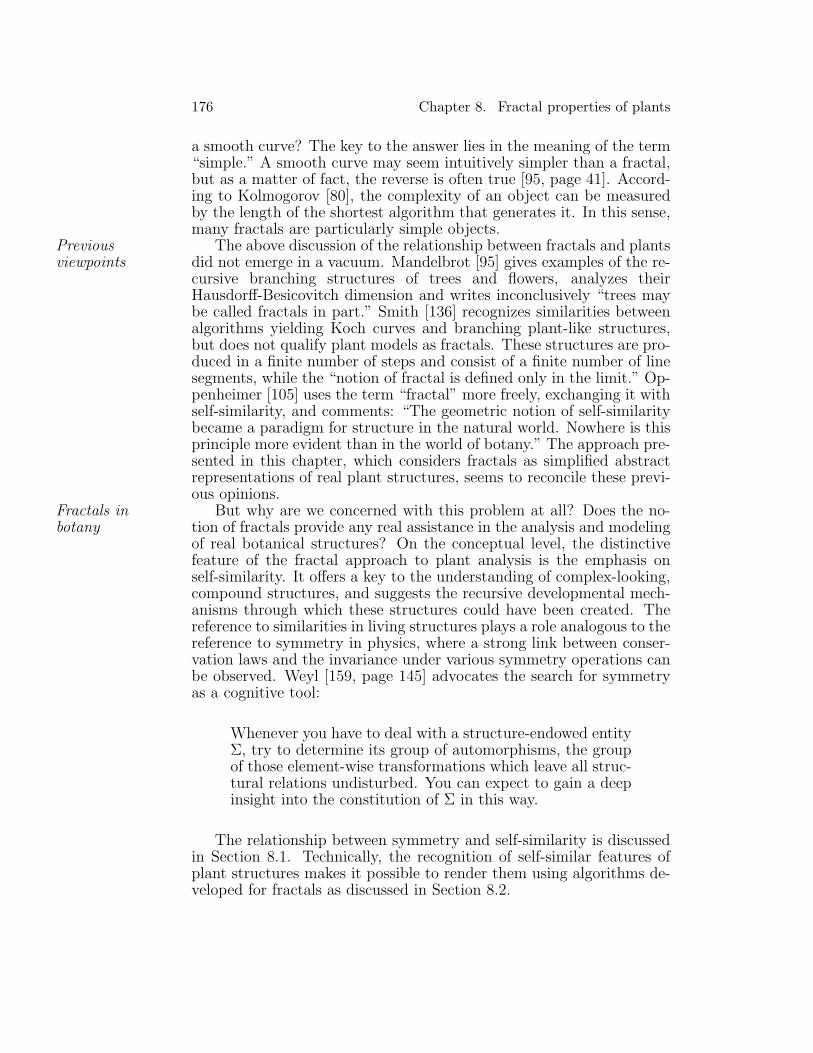
Figure 8.1: The Sierpinski gasket is closed with respect to transformationsT1, T2 and T3 (a), but it is not closed with respect to the set including theinverse transformations (b).

8.1 Symmetry and self-similarity

The notion of symmetry is generally defined as the invariance of a con-figuration of elements under a group of automorphic transformations.Commonly considered transformations are congruences, which can beobtained by composing rotations, reflections and translations. Couldwe extend this list of transformations to similarities, and consider self-similarity as a special case of symmetry involving scaling operations?

On the surface, this seems possible. For example, Weyl [159, page 68]suggests: “In dealing with potentially infinite patterns like band orna-ments or with infinite groups, the operation under which a pattern isinvariant is not of necessity a congruence but could be a similarity.”The spiral shapes of the shells Turritella duplicata and Nautilus aregiven as examples. However, all similarities involved have the samefixed point. The situation changes dramatically when similarities withdifferent fixed points are considered. For example, the Sierpinski gasketis mapped onto itself by a set of three contractions T1, T2 and T3 (Fig-ure 8.1a). Each contraction takes the entire figure into one of its threemain components. Thus, if A is an arbitrary point of the gasket, andT = Ti1Ti2 . . . Tin is an arbitrary composition of transformations T1, T2

and T3, the image T (A) will belong to the set A. On the other hand,if the inverses of transformations T1, T2 and T3 can also be includedin the composition, one obtains points that do not belong to the set Anor its infinite extension (Figure 8.1b). This indicates that the set oftransformations that maps A into itself forms a semigroup generatedby T1, T2 and T3, but does not form a group. Thus, self-similarity is aweaker property than symmetry, yet it still provides a valuable insightinto the relationships between the elements of a structure.


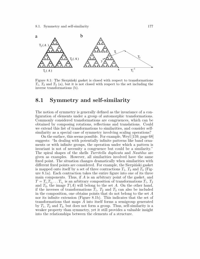
Figure 8.2: The fern leaf from Barnsley’s model [7]

8.2 Plant models and iterated function sys-

tems

Barnsley [7, pages 101–104] presents a model of a fern leaf (Figure 8.2),generated using an iterated function system, or IFS. This raises a ques-tion regarding the relationship between developmental plant modelsexpressed using L-systems and plant-like structures captured by IFSes.This section briefly describes IFSes and introduces a method for con-structing those which approximate structures generated by a certaintype of parametric L-system. The restrictions of this method are ana-lyzed, shedding light on the role of IFSes in the modeling of biologicalstructures.

By definition [74], a planar iterated function system is a finite setIFS definitionof contractive affine mappings T = {T1, T2, . . . , Tn} which map theplane R×R into itself. The set defined by T is the smallest nonemptyset A, closed in the topological sense, such that the image y of anypoint x ∈ A under any of the mappings Ti ∈ T also belongs to A.It can be shown that such a set always exists and is unique [74] (seealso [118] for an elementary presentation of the proof). Thus, startingfrom an arbitrary point x ∈ A, one can approximate A as a set ofimages of x under compositions of the transformations from T . On

8.2. Plant models and iterated function systems 179

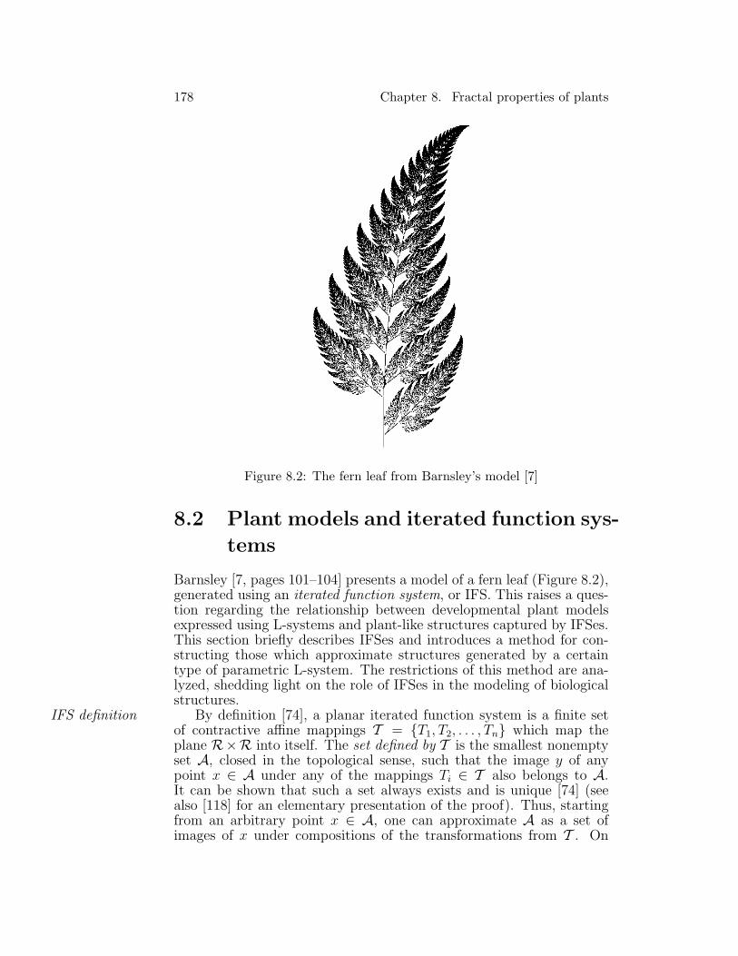
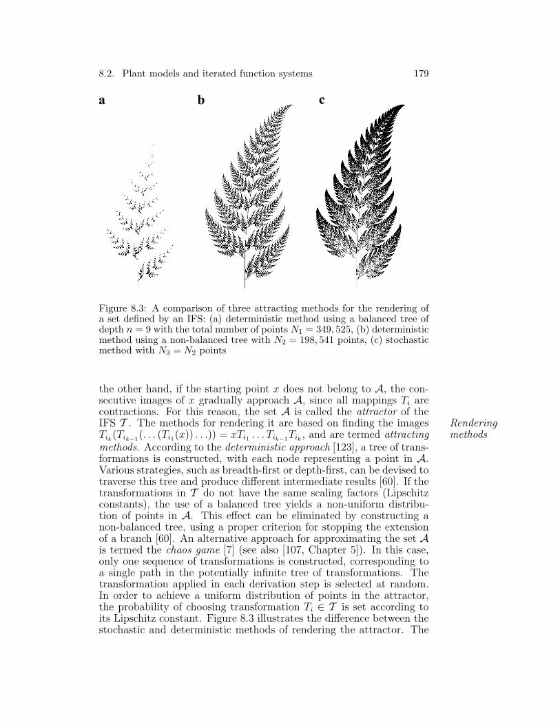
Figure 8.3: A comparison of three attracting methods for the rendering ofa set defined by an IFS: (a) deterministic method using a balanced tree ofdepth n = 9 with the total number of points N1 = 349, 525, (b) deterministicmethod using a non-balanced tree with N2 = 198, 541 points, (c) stochasticmethod with N3 = N2 points

the other hand, if the starting point x does not belong to A, the con-secutive images of x gradually approach A, since all mappings Ti arecontractions. For this reason, the set A is called the attractor of theIFS T . The methods for rendering it are based on finding the images Rendering

methodsTik(Tik−1(. . . (Ti1(x)) . . .)) = xTi1 . . . Tik−1

Tik , and are termed attractingmethods. According to the deterministic approach [123], a tree of trans-formations is constructed, with each node representing a point in A.Various strategies, such as breadth-first or depth-first, can be devised totraverse this tree and produce different intermediate results [60]. If thetransformations in T do not have the same scaling factors (Lipschitzconstants), the use of a balanced tree yields a non-uniform distribu-tion of points in A. This effect can be eliminated by constructing anon-balanced tree, using a proper criterion for stopping the extensionof a branch [60]. An alternative approach for approximating the set Ais termed the chaos game [7] (see also [107, Chapter 5]). In this case,only one sequence of transformations is constructed, corresponding toa single path in the potentially infinite tree of transformations. Thetransformation applied in each derivation step is selected at random.In order to achieve a uniform distribution of points in the attractor,the probability of choosing transformation Ti ∈ T is set according toits Lipschitz constant. Figure 8.3 illustrates the difference between thestochastic and deterministic methods of rendering the attractor. The


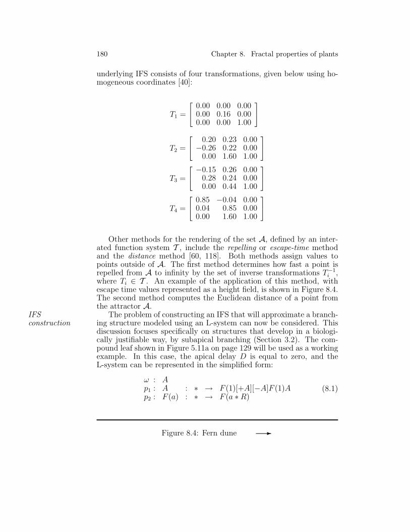
underlying IFS consists of four transformations, given below using ho-mogeneous coordinates [40]:

T1 =

0.00 0.00 0.00

0.00 0.16 0.000.00 0.00 1.00

T2 =

0.20 0.23 0.00−0.26 0.22 0.00

0.00 1.60 1.00

T3 =

−0.15 0.26 0.00

0.28 0.24 0.000.00 0.44 1.00

T4 =

0.85 −0.04 0.00

0.04 0.85 0.000.00 1.60 1.00

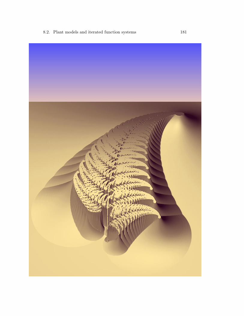
Other methods for the rendering of the set A, defined by an inter-ated function system T , include the repelling or escape-time methodand the distance method [60, 118]. Both methods assign values topoints outside of A. The first method determines how fast a point isrepelled from A to infinity by the set of inverse transformations T−1

i ,where Ti ∈ T . An example of the application of this method, withescape time values represented as a height field, is shown in Figure 8.4.The second method computes the Euclidean distance of a point fromthe attractor A.

The problem of constructing an IFS that will approximate a branch-IFSconstruction ing structure modeled using an L-system can now be considered. This

discussion focuses specifically on structures that develop in a biologi-cally justifiable way, by subapical branching (Section 3.2). The com-pound leaf shown in Figure 5.11a on page 129 will be used as a workingexample. In this case, the apical delay D is equal to zero, and theL-system can be represented in the simplified form:

ω : Ap1 : A : ∗ → F (1)[+A][−A]F (1)Ap2 : F (a) : ∗ → F (a ∗ R)

(8.1)

Figure 8.4: Fern dune �


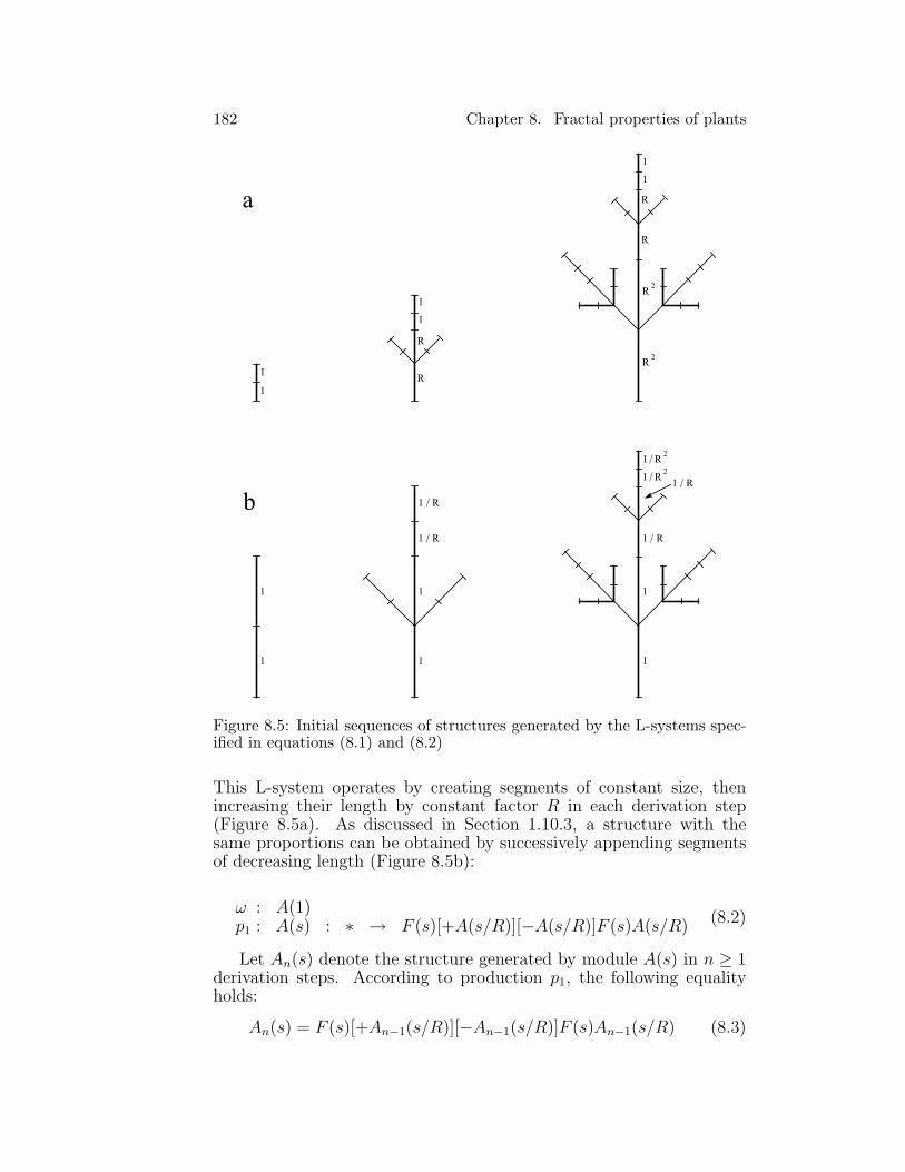
Figure 8.5: Initial sequences of structures generated by the L-systems spec-ified in equations (8.1) and (8.2)

This L-system operates by creating segments of constant size, thenincreasing their length by constant factor R in each derivation step(Figure 8.5a). As discussed in Section 1.10.3, a structure with thesame proportions can be obtained by successively appending segmentsof decreasing length (Figure 8.5b):

ω : A(1)p1 : A(s) : ∗ → F (s)[+A(s/R)][−A(s/R)]F (s)A(s/R) (8.2)

Let An(s) denote the structure generated by module A(s) in n ≥ 1derivation steps. According to production p1, the following equalityholds:

An(s) = F (s)[+An−1(s/R)][−An−1(s/R)]F (s)An−1(s/R) (8.3)


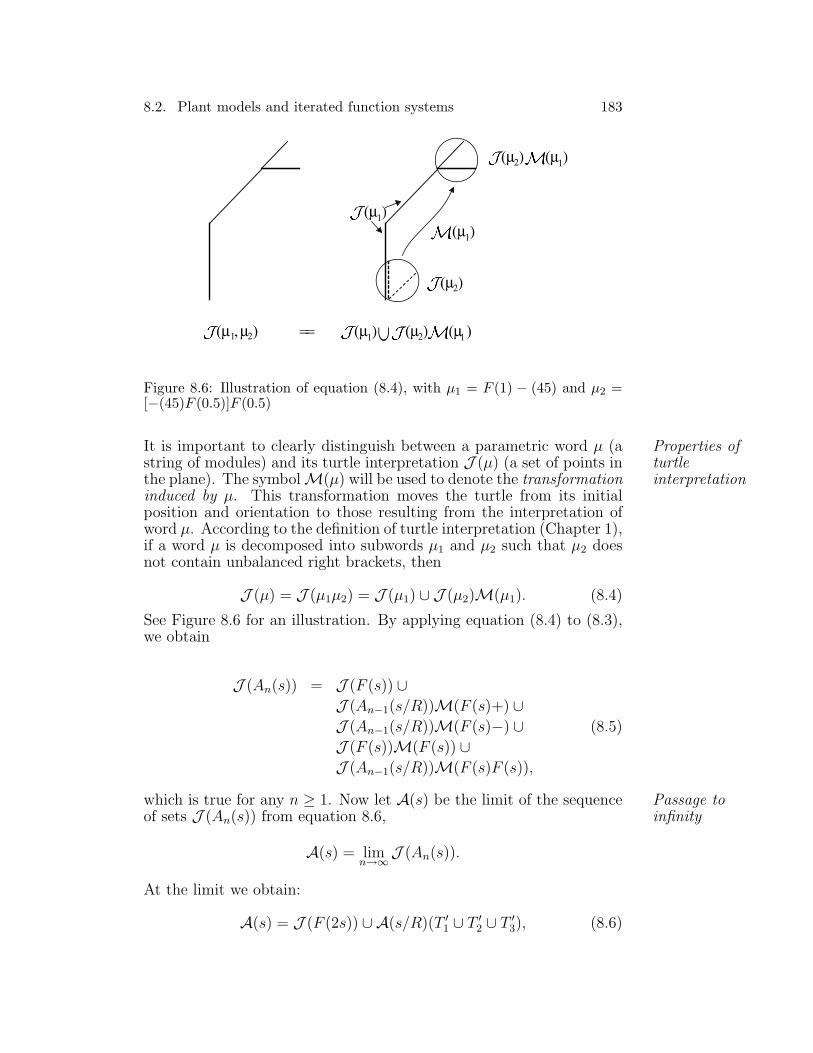
Figure 8.6: Illustration of equation (8.4), with µ1 = F (1) − (45) and µ2 =[−(45)F (0.5)]F (0.5)

It is important to clearly distinguish between a parametric word µ (a Properties ofturtleinterpretation

string of modules) and its turtle interpretation J (µ) (a set of points inthe plane). The symbol M(µ) will be used to denote the transformationinduced by µ. This transformation moves the turtle from its initialposition and orientation to those resulting from the interpretation ofword µ. According to the definition of turtle interpretation (Chapter 1),if a word µ is decomposed into subwords µ1 and µ2 such that µ2 doesnot contain unbalanced right brackets, then

J (µ) = J (µ1µ2) = J (µ1) ∪ J (µ2)M(µ1). (8.4)

See Figure 8.6 for an illustration. By applying equation (8.4) to (8.3),we obtain

J (An(s)) = J (F (s)) ∪J (An−1(s/R))M(F (s)+) ∪J (An−1(s/R))M(F (s)−) ∪ (8.5)

J (F (s))M(F (s)) ∪J (An−1(s/R))M(F (s)F (s)),

which is true for any n ≥ 1. Now let A(s) be the limit of the sequence Passage toinfinityof sets J (An(s)) from equation 8.6,

A(s) = limn→∞J (An(s)).

At the limit we obtain:

A(s) = J (F (2s)) ∪ A(s/R)(T ′1 ∪ T ′2 ∪ T ′3), (8.6)


where T ′1 = T (F (s)+), T ′2 = T (F (s)−), and T ′3 = T (F (2s)). LetS(s/R) be the operation of scaling by s/R, then

A(s/R) = A(s)S(s/R).

By noting Ti = T ′iS(s/R) for i = 1, 2, 3, equation (8.6) can be trans-formed to

A(s) = J (F (2s)) ∪ A(s)(T1 ∪ T2 ∪ T3). (8.7)

The solution of this equation with respect to A(s) is

A(s) = J (F (2s))(T1 ∪ T2 ∪ T3)∗, (8.8)

where (T1 ∪ T2 ∪ T3)∗ stands for the iteration of the union of transfor-

mations T1, T2 and T3. Equation (8.8) suggests the following methodfor constructing the set (A(s)):

• create segment J (F (2s))

• create images of J (F (2s)) using transformations T1, T2, T3 andtheir compositions

Equation (8.7) and the method of constructing the set A(s) basedon equation (8.8) are closely related to the definition of iterated functionsystems stated at the beginning of this chapter. However, instead ofstarting from an arbitrary point x ∈ A(s), the iteration begins withthe set J (F (2s)). Although this is simply a straight line segment, aquestion arises as to how its generation can be incorporated into anIFS. Two approaches can be distinguished.

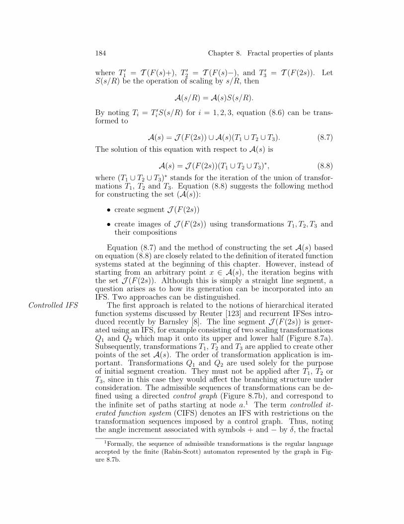
The first approach is related to the notions of hierarchical iteratedControlled IFSfunction systems discussed by Reuter [123] and recurrent IFSes intro-duced recently by Barnsley [8]. The line segment J (F (2s)) is gener-ated using an IFS, for example consisting of two scaling transformationsQ1 and Q2 which map it onto its upper and lower half (Figure 8.7a).Subsequently, transformations T1, T2 and T3 are applied to create otherpoints of the set A(s). The order of transformation application is im-portant. Transformations Q1 and Q2 are used solely for the purposeof initial segment creation. They must not be applied after T1, T2 orT3, since in this case they would affect the branching structure underconsideration. The admissible sequences of transformations can be de-fined using a directed control graph (Figure 8.7b), and correspond tothe infinite set of paths starting at node a.1 The term controlled it-erated function system (CIFS) denotes an IFS with restrictions on thetransformation sequences imposed by a control graph. Thus, notingthe angle increment associated with symbols + and − by δ, the fractal

1Formally, the sequence of admissible transformations is the regular languageaccepted by the finite (Rabin-Scott) automaton represented by the graph in Fig-ure 8.7b.


Figure 8.7: Construction of the set A(S): (a) definition of an IFS {Q1, Q2}that generates the initial line segment, (b) the control graph specifying theadmissible sequences of transformation application

approximation of the leaf in Figure 5.11a is given by the CIFS with the Resulting CIFScontrol graph in Figure 8.7b and the transformations specified below:

Q1 =

0.5 0 0

0 0.5 00 0 1

Q2 =

0.5 0 0

0 0.5 00 s 1

T1 =

1/R cos δ 1/R sin δ 0

−1/R sin δ 1/R cos δ 00 s 1

T2 =

1/R cos δ −1/R sin δ 0

1/R sin δ 1/R cos δ 00 s 1

T3 =

1/R 0 0

0 1/R 00 2s 1

The second approach to the generation of the line segment J (F (2s)) Noninvertibletransforma-tions

is consistent with the method applied by Barnsley to specify the fernleaf in Figure 8.2. The idea is to map the entire branching structureA(s) onto the line J (F (2s)). This can be achieved using a noninvertibletransformation Q which collapses all branches into a vertical line. Thescaling factor along the y axis is the ratio of the desired segment length2s, and the limit height of the entire structure A(s),

h =2s

1 − 1/R.


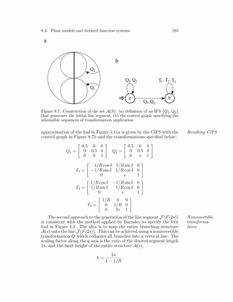
Figure 8.8: Two renderings of the compound leaf from Figure 5.11a, gener-ated using iterated function systems

This last value is calculated as the limit of the geometric series with thefirst term equal to 2s and the ratio equal to 1/R. Thus, the compoundleaf of Figure 5.11a is defined by an IFS consisting of transformation

Q =

0 0 0

0 1 − 1/R 00 0 1

and transformations T1, T2 and T3 specified as in the case of the con-trolled IFS.

Two fractal-based renderings of the set A(s) are shown in Fig-Renderingexamples ure 8.8. Figure 8.8a was obtained using the controlled IFS and a deter-

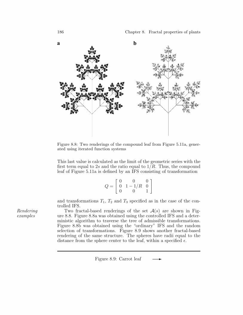
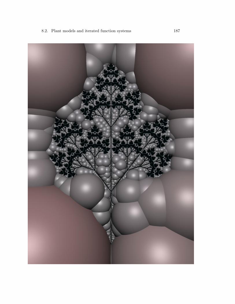
ministic algorithm to traverse the tree of admissible transformations.Figure 8.8b was obtained using the “ordinary” IFS and the randomselection of transformations. Figure 8.9 shows another fractal-basedrendering of the same structure. The spheres have radii equal to thedistance from the sphere center to the leaf, within a specified ε.

Figure 8.9: Carrot leaf �


L-system with elongating internodes

‖L-system transformation

⇓L-system with decreasing apices

‖L-system analysis

⇓Recurrent equation in the domain of strings

‖Graphical interpretation

⇓Recurrent equation in the domain of sets

‖Passage to limit

⇓An equation expressing the limit set as a union ofthe limit object and reduced copies of itself

‖Equation solution

⇓An equation expressing the limit object as the im-age of an initial object under an iteration of aunion of transformations

‖Elimination of the initial object

⇓A (controlled) IFS

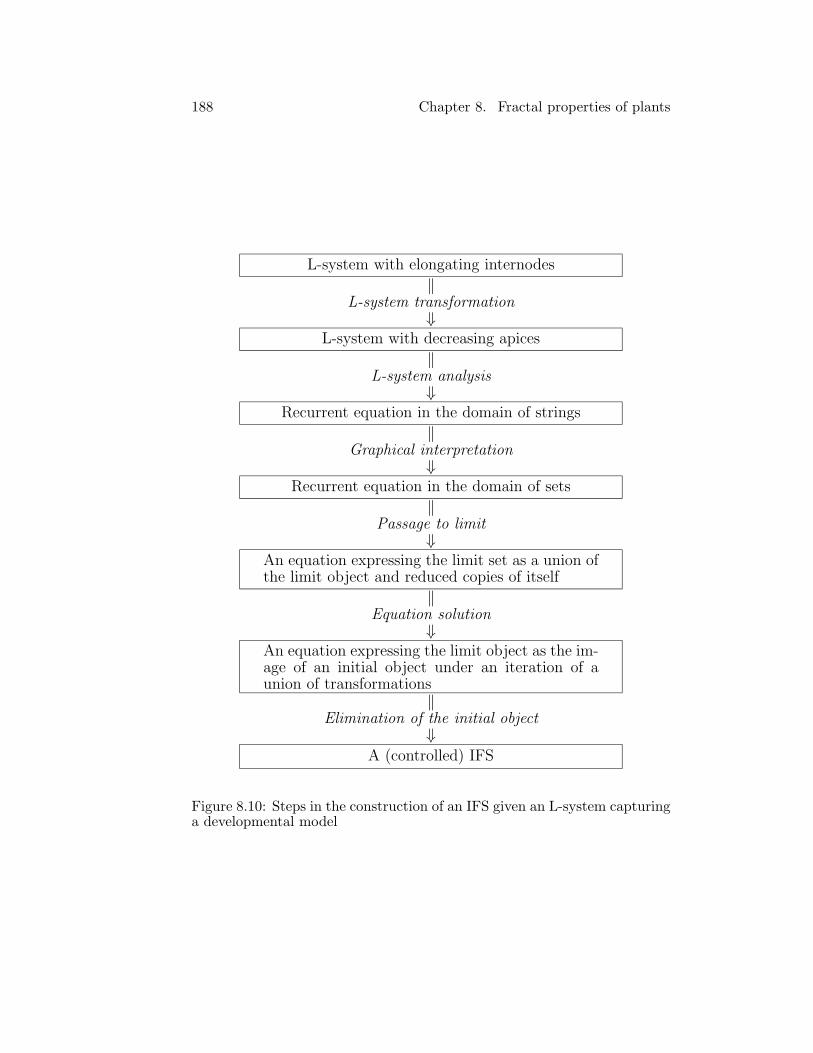
Figure 8.10: Steps in the construction of an IFS given an L-system capturinga developmental model


It is instructive to retrace the logical construction that started with Conclusionsan L-system, and ended with an iterated function system which cangenerate fractal approximations of the same object (Figure 8.10). Ananalysis of the operations performed in the subsequent steps of thisconstruction reveals its limitations, and clarifies the relationship be-tween strictly self-similar structures and real plants. The critical stepis the transformation of the L-system with elongating internodes to theL-system with decreasing apices. It can be performed as indicated inthe example if the plant maintains constant branching angles as well asfixed proportions between the mother and daughter segments, indepen-dent of branch order. This, in turn, can be achieved if all segments inthe modeled plant elongate exponentially over time. These are strongassumptions, and may be satisfied to different degrees in real plants.Strict self-similarity is an abstraction that captures the essential prop-erties of many plant structures and represents a useful point of referencewhen describing them in detail.

Epilogue

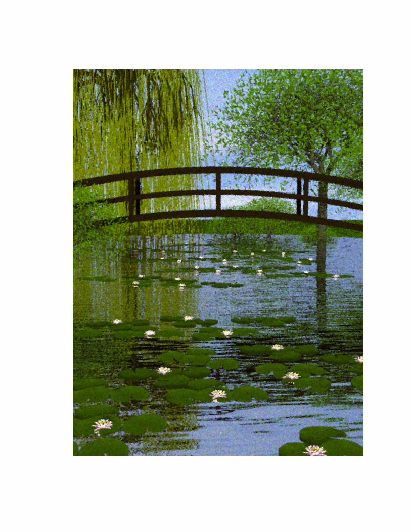
This quiet place, reminiscient of Claude Monet’s 1899 painting Water-lilies pool — Harmony in green, does not really exist. The scene wasmodeled using L-systems that captured the development of trees andwater plants, and illuminated by simulated sunlight. It is difficult notto appreciate how far the theory of L-systems and the entire field ofcomputer graphics have developed since their beginnings in the 1960’s,making such images possible. Yet the results contained in this book arenot conclusive and constitute only an introduction to the research onplant modeling for biological and graphics purposes. The algorithmicbeauty of plants is open to further exploration.

� Figure E.1: Water-lilies

chapter 8 fractal properties of plants - algorithmic...

Documents