chapter 7 trading stochastic production in electricity...

Chapter 7Trading Stochastic Production in ElectricityPools

7.1 Introduction and Decision Framework

Recent years have witnessed an exceptional technological development that, alongwith increasing political pressure to cut CO2 emissions and to create local jobs,spurred an unprecedented growth in installed production capacity from renewablesources. To sustain such growth, national governments have put in place specialsupport schemes (tax credits, feed-in tariffs, etc.) for easing the market participationof renewable producers.

As the energy cost of renewables constantly decreases approaching grid parity,green power needs smaller and smaller incentives for being competitive. For thisreason, renewable power producers are increasingly required to participate in elec-tricity markets under the same rules as conventional power producers. In particular,as opposed to feed-in tariff schemes, they are more and more frequently subject tomarket prices and assigned balance responsibility. The former implies that renew-able electricity producers are subject, like any other power producer, to price risk.Besides, the latter implies that they are financially accountable for the additionalbalancing costs incurred by the system operators, which in practice means that theyneed to correct their energy imbalances by trading in the balancing market.

Although renewable producers are asked to participate in the market in the sameway as conventional producers, trading green energy presents substantial differenceswhen compared to the case of conventional power sources. Firstly, the actual produc-tion is variable and uncertain at the time of offering. This uncertainty, coupled withthe stochastic nature of power prices, results in uncertain returns depending on therealization of both power production and prices. Secondly, renewable producers areforced to participate in multiple markets, because markets with early gate closures—day-ahead- markets—have more stable prices and, in parallel, deviations of the actualproduction from the contractual positions at the day-ahead and adjustment marketsmust be settled at the balancing market.

As the market design often—although not always—penalizes real-time devia-tions from (and in general later corrections of) the day-ahead schedule, renewablepower producers are in a disadvantaged position compared to conventional producers.As a partial solution to these disadvantages, renewable power producers can trade

J. M. Morales et al., Integrating Renewables in Electricity Markets, 205International Series in Operations Research & Management Science 205,DOI 10.1007/978-1-4614-9411-9_7, © Springer Science+Business Media New York 2014

206 7 Trading Stochastic Production in Electricity Pools

strategically, in the attempt to get the most out of the information they possess onthe uncertain variables in play. This chapter focuses on the determination of optimaltrading strategies for renewable power producers participating in electricity pools.Owing to the stochastic features and the multiple market layers described above, thisis a multistage problem of decision-making under uncertainty.

Two basic assumptions are made in this chapter. The first one entails that incen-tives such as price premia added on top of market prices, feed-in tariffs, etc., arediscarded. As a result, renewable energy is traded under exactly the same rules asthe conventional one. This simplification is introduced for the sake of clarity andgenerality as different markets have different incentive schemes. Nevertheless, thetools developed here could be extended so as to account for these incentives withlittle effort. The second assumption is that renewable power producers participatein the electricity pool on their own. This means that the optimal trading strategiesdeveloped in this chapter do not account for possible associations with other marketentities, e.g., owners of storage devices or flexible demand, which are treated inChaps. 8 and 9, respectively.

This chapter is structured as follows. Section 7.2 presents the basic problemformulation and introduces some common concepts in decision-making under un-certainty. Optimal strategies are determined analytically in Sect. 7.3 for offering inthe day-ahead and balancing markets considering deterministic electricity prices.Section 7.4 develops different strategies in a series of cases with stochastic marketprices. Section 7.5 considers the case of a risk-averse stochastic producer. Thereafter,Sect. 7.6 models the problem in the framework of stochastic programming, which ismore versatile as it can accommodate any type of probabilistic multivariate distribu-tion of the uncertainty as well as different risk metrics. Finally, Sect. 7.7 concludesthe chapter.

7.2 Revenue and Imbalance Cost: Concept and Definition

In this section, we introduce the basic formulation of the problem of optimal tradingwhen the production volume is uncertain, which is the case for renewable energysources such as wind and solar. In parallel, some concepts of decision-making underuncertainty are presented.

In order to set up the problem in a simple framework, we introduce the followingassumptions. Later on in the development of this chapter, assumptions A1–A3 willbe gradually removed.

A1 The stochastic producer trades only at the day-ahead and at the balancing market,while adjustment markets are discarded from the analysis.

A2 The only uncertainty is related to the production volume, while market pricesare deterministic and known in advance.

A3 The producer is risk-neutral, meaning that it aims at the maximization of theexpected profits with disregard of possible losses.

A4 The stochastic producer is a price-taker, i.e., market prices do not depend on theemployed offering strategy.

7.2 Revenue and Imbalance Cost: Concept and Definition 207

Assumptions A1 and A4 are critical for obtaining an analytical solution to the tradingproblem. On the other hand, assumption A2, which is exploited in the derivations inSect. 7.3, is mainly for presentation convenience. Indeed, Sect. 7.4.1 shows that, un-der the assumption that production and market prices are uncorrelated, prices can besubstituted by their expected values. Analytical solutions are still available under lessrestrictive assumptions on the correlation between day-ahead and balancing marketprices; they are presented in Sect. 7.4.1. Further results obtained considering thecorrelation between prices and production are presented in [6]. The risk-neutralityassumption A3 is justified by the relatively high frequency with which the produc-ers offer in electricity markets. This implies that the possible losses incurred ina single trading period are small if aggregated over a reasonable time-span. Sec-tion 7.5 presents some analytical results available when considering a risk-aversepower producer.

As we show in Sect. 7.6, the stochastic programming framework provides thenecessary flexibility to treat the trading problem for stochastic power producersdisregarding the assumptions A1–A3 above.

To get rid of the price-taker assumption A4, one can employ mathematical pro-grams with equilibrium constraints (MPEC), see Appendix B and [7]. Given itscomplexity, this topic is not covered here. However, we refer the interested reader to[2] and [18], where stochastic MPECs are applied to trading problems of renewablesuppliers.

In the remainder of this section, we consider the cases of one-price and two-pricemarkets separately.

Before getting started, two important clarifications should be made. Firstly, weassume that the renewable electricity producer is located at a certain bus of thetransmission network. For the sake of simplicity, we always use the term “marketprice.” However, if considering a market with nodal pricing, “market price” hasthe meaning of “locational marginal price (LMP) at the bus of interest.” Similarlyin a market with zonal pricing, such term would refer to the relevant zonal price.Notice that the generalization of the models presented in this chapter to the case of aproducer whose plants are located in different nodes, or zones, of the power networkis straightforward.

Secondly, there are no intertemporal constraints in the problems we analyze. Thismeans that we focus on single-period models, and thus time indexes are droppedfrom the mathematical formulations.

7.2.1 One-Price Market

In a one-price balancing market, deviations from day-ahead contracts are traded ata unique balancing price regardless of the sign of producer and system imbalances.Generally, the balancing market price is higher than the day-ahead price if the systemis in up-regulation, i.e., when the system is in deficit of power production as a resultof all the deviations from producers and consumers with respect to their day-ahead


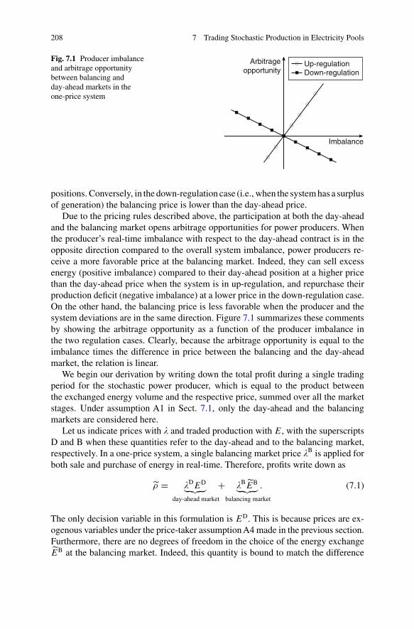
Fig. 7.1 Producer imbalanceand arbitrage opportunitybetween balancing andday-ahead markets in theone-price system

Up-regulationDown-regulation

Imbalance

Arbitrageopportunity

positions. Conversely, in the down-regulation case (i.e., when the system has a surplusof generation) the balancing price is lower than the day-ahead price.

Due to the pricing rules described above, the participation at both the day-aheadand the balancing market opens arbitrage opportunities for power producers. Whenthe producer’s real-time imbalance with respect to the day-ahead contract is in theopposite direction compared to the overall system imbalance, power producers re-ceive a more favorable price at the balancing market. Indeed, they can sell excessenergy (positive imbalance) compared to their day-ahead position at a higher pricethan the day-ahead price when the system is in up-regulation, and repurchase theirproduction deficit (negative imbalance) at a lower price in the down-regulation case.On the other hand, the balancing price is less favorable when the producer and thesystem deviations are in the same direction. Figure 7.1 summarizes these commentsby showing the arbitrage opportunity as a function of the producer imbalance inthe two regulation cases. Clearly, because the arbitrage opportunity is equal to theimbalance times the difference in price between the balancing and the day-aheadmarket, the relation is linear.

We begin our derivation by writing down the total profit during a single tradingperiod for the stochastic power producer, which is equal to the product betweenthe exchanged energy volume and the respective price, summed over all the marketstages. Under assumption A1 in Sect. 7.1, only the day-ahead and the balancingmarkets are considered here.

Let us indicate prices with � and traded production with E, with the superscriptsD and B when these quantities refer to the day-ahead and to the balancing market,respectively. In a one-price system, a single balancing market price �B is applied forboth sale and purchase of energy in real-time. Therefore, profits write down as

ρ = �DED︸︷︷︸

day-ahead market

+ �BEB︸︷︷︸

balancing market

. (7.1)

The only decision variable in this formulation is ED. This is because prices are ex-ogenous variables under the price-taker assumption A4 made in the previous section.Furthermore, there are no degrees of freedom in the choice of the energy exchangeEB at the balancing market. Indeed, this quantity is bound to match the difference

7.2 Revenue and Imbalance Cost: Concept and Definition 209

between the day-ahead schedule and the actual production, i.e.,

EB = E − ED. (7.2)

Being dependent on the uncertain production E, the real-time exchange EB isstochastic, and so is the profit.

A relevant question when a decision-maker is exposed to stochastic profits isthe definition of the objective of the optimal strategy. Owing to the risk-neutralityassumption A3, the producer is in this case interested in maximizing its profitsin expectation, regardless of whether the shape of the profit distribution entails thepossibility of incurring large losses. As we discuss in the following sections, decision-makers are not always risk-neutral, since in some circumstances possible losses arelarge enough to cause them financial problems.

In decision theory, the expected value of the profits for a certain decision goesunder the name of expected monetary value (EMV). Replacing (7.2) into (7.1), andtaking the expectation yields the following expression for the EMV:

E {ρ} = (�D − �B)ED + �B

E, (7.3)

where E is the expected value of power production in the trading period considered.

7.2.2 Two-Price Market

In a two-price market, real-time deviations are priced differently depending on theimbalance sign. Deviations that are in the opposite direction to the overall systemimbalance, which help the system restore the balance between production and con-sumption, are priced at the day-ahead market price. On the contrary, imbalances ofthe same sign as that of the system are settled at the clearing price of the balancingmarket. Let us denote the up-regulation and down-regulation prices with �UP and�DW, respectively, while the clearing price at the balancing market is still �B. Thepricing rule in a two-price balancing market implies the following

�UP ={

�B if �B ≥ �D,

�D if �B< �D,

(7.4)

�DW ={

�D if �B ≥ �D,

�B if �B< �D

.(7.5)

As Fig. 7.2 shows, and contrarily to the one-price system, there is no arbitrageopportunity when the producer deviation is in the opposite direction to the overallsystem imbalance, since the price obtained at the balancing market is equal to theday-ahead market price. On the contrary, there is still an opportunity loss whenproducer and system deviations have the same sign.


Fig. 7.2 Producer imbalanceand arbitrage opportunitybetween balancing andday-ahead markets in thetwo-price system

Up-regulationDown-regulation

Imbalance

Arbitrageopportunity

As a result of this pricing rule, the term accounting for the balancing market profitin (7.1) splits in two when considering such a market settlement, resulting in thefollowing formulation for the total profits

ρ = �DED︸︷︷︸

day-ahead market

+ �UPEUP + �DW

EDW︸︷︷︸balancing market

. (7.6)

The symbols EUP and EDW refer to energy up-regulation and down-regulation forthe producer at the balancing market, respectively. We recall that the power producerhas to purchase upward regulation power at the balancing market when its actualproduction E is lower than the day-ahead position, ED, while downward regulationis to be sold when E is larger than ED. In mathematical terms, this writes

EUP ={

E − ED if E − ED ≤ 0,

0 if E − ED > 0,(7.7)

EDW ={

0 if E − ED ≤ 0,

E − ED if E − ED > 0.(7.8)

From the definition of up-regulation and down-regulation, it follows that

E − ED = EUP + EDW. (7.9)

Solving the previous equation for ED and substituting the resulting expression in(7.6) yields

ρ = �DE − [(�D − �UP)

EUP + (�D − �DW)EDW

]. (7.10)

We notice that the first term of the sum in (7.10) is not under control of the powerproducer, in that neither �D nor E are dependent on its decisions. Furthermore, bothterms inside brackets are nonnegative. This is because in a two-price system, pricingrules (7.4) and (7.5) entail that �UP ≥ �D and �DW ≤ �D, and because (7.7) and (7.8)imply that EUP ≤ 0 and EDW ≥ 0.

7.3 Trading with Deterministic Prices: Bidding Quantities 211

The first term in (7.10) represents the profit that could be obtained by the producer,in a two-price system, if it had perfect information on the future realization of thestochastic production E. Clearly in this case, the producer would sell the (certain)production entirely at the day-ahead market, since as Fig. 7.2 shows there is nevera strictly positive arbitrage opportunity between the balancing market and the day-ahead one. The term within brackets in (7.10) is the imbalance costs that the producerfaces when settling its regulation volume at the balancing market. This sum representsan opportunity loss, in that it quantifies the missing profits stemming from not beingable to sell the uncertain production entirely, or for selling more than the actualproduction, at the day-ahead market.

Taking the expectation on both sides of (7.10), we get the following

E {ρ}︸︷︷︸EMV

= �DE − E

{(�D − �UP)

EUP + (�D − �DW)EDW

}︸︷︷︸

EOL

, (7.11)

where E is the expected power production and therefore, �DE is the expected profit

given perfect information. We will refer to the expectation term on the right-hand sideof (7.11) equivalently as the expected imbalance costs or as the expected opportunityloss (EOL).

Equation (7.11) states a general fact of decision-making under uncertainty: forany strategy, the sum of the expected monetary value (EMV) and the EOL is constantand equal to the expected profit obtained with perfect information. Therefore, wecan alternatively look at the optimal strategy of a risk-neutral decision-maker eitheras the strategy maximizing the EMV, or as the decision minimizing the EOL. In thenext section, we will determine the optimal offer for a stochastic power producer inthe two-price system by formulating the problem as the minimization of the EOL.

As a final remark of this section, we point out that the minimum value of the EOLamong all the feasible decisions is of particular importance. Such quantity is referredto as the expected value of perfect information (EVPI) . The EVPI represents the profitimprovement that the decision-maker would experience if it held perfect informationon the realization of the uncertainty, compared to the best performance achievablewith the employed characterization of the stochastic parameters. Hence, this quantityalso indicates how much the decision-maker would pay at most for obtaining perfectinformation on the contingent process. As such, the EVPI represents an upper boundto the value of an improved forecasting model for the uncertainty.

7.3 Trading with Deterministic Prices: Bidding Quantities

This section presents some analytical results for the determination of optimal tradingstrategies for stochastic producers when market prices are deterministic, i.e., knownin advance with certainty. Similarly to the previous section, results for the one-priceand the two-price markets are presented separately.


7.3.1 One-Price Market

The final result in Sect. 7.2.1 was the formulation (7.3) for the expected profitsof a stochastic power producer in a one-price market. Equation (7.3) reveals thetriviality of the determination of the optimal offer in a one-price system when pricesare deterministic. Indeed, the second term on the right-hand side of (7.3) does notdepend on the producer’s decision. Therefore, this constant term can be discardedfrom the determination of the optimum. As far as the optimization of the first termis concerned, the following cases can happen, all with a trivial solution.

1. If �D< �B, the power producer sells nothing at the day-ahead market, and waits

to place all its production at the balancing market, where the price �B is higher.2. If �D

> �B, the power producer sells as much energy as possible at the day-aheadmarket, eventually buying back at the balancing market the energy needed to coverthe difference between day-ahead trade and actual production (7.2). As �B

< �D,the producer realizes a surplus on the energy that is sold at the day-ahead marketbut not delivered.

3. If �D = �B, the power producer is indifferent since any decision on ED wouldyield the same profit.

Given that, in electricity markets, producers are usually imposed not to offer abovetheir installed capacity E, we have the following result.

In a one-price system, under the assumption of deterministic market prices,the optimal offer for a risk-neutral stochastic power producer is price-inelasticand equal to zero volume if the balancing price is higher than the day-aheadprice, while it is equal to the nominal capacity E if the balancing price is lowerthan the day-ahead price; if such prices are equal, any offer is optimal.

The expression “price-inelastic” in the previous sentence means that the optimal offeris either zero or the nominal capacity, regardless of the value of the day-ahead price.As we shall see in Sect. 7.4.2, this is particularly meaningful as market rules allowproducers to specify their offer as a price-quantity curve.

The solution obtained in this simplified case is trivial and, besides, completely de-coupled from the forecast of the stochastic power production, as it is only dependenton the forecast of the arbitrage opportunity between the day-ahead and the balancingmarkets.

Furthermore, it should be pointed out that the statement that the rightmost termin (7.3) is not under the control of the power producer is not completely true. Inprinciple, power producers could spill their excess production if economically at-tractive. This has little impact on the optimal day-ahead strategy described above,but it would imply that, should the price �B be negative, the producer would ratherspill its power production and gain additional profits when repurchasing power.

7.3 Trading with Deterministic Prices: Bidding Quantities 213

7.3.2 Two-Price Market

It is relevant to recall that the optimal strategy for a risk-neutral stochastic producerminimizes the expected imbalance costs, i.e., the EOL in (7.11). Before carrying outthe necessary algebra, we define the following penalties, both nonnegative

ψUP =�UP − �D, (7.12)

ψDW =�D − �DW. (7.13)

It is important to notice that ψUP and ψDW represent the opportunity loss per energyunit, i.e., the profits lost by exchanging up-regulation and down-regulation energyat the balancing market instead of at the day-ahead stage. Substituting the abovequantities in the EOL term in (7.11), we get the following expression

EOL = E{−ψUPEUP + ψDWEDW

}. (7.14)

We determine the optimal day-ahead offer in the following way: first, we expand theexpectation in (7.14) into an integral in the probability space of uncertain production;then, the first-order stationarity condition is enforced.

The terms inside the expectation operator in (7.14) can be expanded. Owing tothe piecewise definitions of up-regulation and down-regulation in (7.7) and (7.8),respectively, each term in (7.14) expands into an integration in a half-space of the setof feasible day-ahead offers

[0, E

], split in two halves by the day-ahead offer ED,

i.e.,

EOL = −∫ ED

0ψUP

(E − ED

)pE(E)dE +

∫ E

EDψDW

(E − ED

)pE(E)dE,

(7.15)

where pE( · ) is the probability density function (pdf) of the stochastic power produc-tion E. The reader is referred to Appendix A for an introduction to random variablesand to the concept of probability density function.

To determine the optimum, we enforce the first-order stationarity condition bytaking the derivative of expression (7.15) with respect to the day-ahead offer ED andsetting it equal to 0. Carrying out the differentiation under the integral sign, see [9],yields the following

dEOL

dED= − ψUP

∫ ED

0−pE(E)dE + ψDW

∫ E

ED−pE(E)dE

=ψUPFE(ED) + ψDW(FE(ED) − 1

) = 0, (7.16)

where FE( · ) indicates the cumulative distribution function (cdf) of power produc-tion, see Appendix A. Solving (7.16) for the day-ahead offer ED readily yields thefollowing expression

ED∗ = F−1E

(ψDW

ψUP + ψDW

), (7.17)


which involves the inverse F−1E

( · ) of the production cdf, i.e., the quantile function,

which is defined in Appendix A. The optimality of ED∗ in (7.17) can be easilychecked by noticing that the second order derivative of EOL with respect to ED isnonnegative everywhere

d2EOL

dED2 (ED) = ψUPpE(ED) + ψDWpE(ED) ≥ 0. (7.18)

This is because probability density functions are nonnegative by definition, and soare the penalties according to (7.12) and (7.13). As a consequence of (7.18) and undermild continuity assumptions, the EOL is convex with respect to ED, which impliesthat the first-order stationarity condition (7.16) is sufficient to ensure that ED∗ is aminimum. The results obtained so far can be summarized in the following statement.

In a two-price system, under the assumption of deterministic market prices,the optimal day-ahead offer for a risk-neutral stochastic power producer isprice-inelastic and equal to the quantile of the power production distributioncorresponding to a probability equal to the down-regulation penalty dividedby the sum of the up-regulation and down-regulation penalties.

Example 7.1 (Optimal bid in a two-price settlement with deterministic prices) Letus consider the following deterministic penalties due to the less favorable price atthe balancing market

ψUP =$9/MWh,

ψDW =$4/MWh.

An analyst provides us with a probabilistic forecast of the stochastic power productionat trading period t of the following day. We refer the reader to Chap. 2 for anintroduction to forecasting the production from renewable sources. According to theanalyst, power production follows a uniform distribution, see Appendix A, between100 MWh and 150 MWh. The cumulative distribution function is therefore

FE(E) =

⎧⎪⎪⎨⎪⎪⎩

0 if E < 100,E − 100

50if 100 ≤ E < 150,

1 if E ≥ 150.

(7.19)

According to (7.17), the optimal offer must satisfy

FE(ED∗) = ψDW

ψUP + ψDW= 4

13, (7.20)

which yields, by inverting the function in the second case in (7.19)

ED∗ = 100 + 50 × 4

13MWh = 115.38 MWh. (7.21)

7.4 Trading with Stochastic Prices 215

Fig. 7.3 Expected imbalancecost (EOL) as a function ofthe day-ahead offer. Theexpected profit is thedifference between theexpected profit with perfectinformation (PI) and the EOL

100 110 120 130 140

100

200

...

6250

Mar

ket r

esul

t [$]

Exp. profit with PIExp. imbalance cost (EOL)

ED*

EOL*

Exp. profit

ED[MWh]

It is worth noticing that this result makes sense also from an intuitive point of view.Indeed, the optimal quantity offer is lower than 125 MWh, which is both the meanand the median of the power production distribution. This is in accordance with thefact that the penalty ψUP for underproducing with respect to the day-ahead marketcontract is higher than the penalty ψDW for overproducing, which makes a longposition at the day-ahead market more attractive.

Figure 7.3 shows the expected imbalance cost (expected opportunity loss) as afunction of the day-ahead offer. According to (7.11), the expected profit obtainedwith a given day-ahead offer ED is the difference between the expected profit withperfect information (PI) and the EOL. The optimal quantity offer ED∗ is a minimumpoint for the expected imbalance cost and, as a consequence, a maximum pointfor the expected profit. Observe that the expected profit with perfect information iscalculated with a day-ahead price �D = $50/MWh.

It is relevant to note that the closed formula (7.17) for the optimal day-aheadoffer rests on the assumption that the cumulative distribution function FE( · ) beinvertible. In fact, we already know that FE( · ) is, by definition of cdf, monotonicallyincreasing, though the monotonicity may be nonstrict. In the latter case, the closedformula (7.17) is still valid using the generalized inverse function

F−1E

(α) = inf{x ∈ [0, E

]: FE(x) ≥ α

}. (7.22)

In fact, any amount ED such that FE(ED) = ψDW/(ψDW + ψUP) is optimal in thiscase.

Finally, we underline that expression (7.17) always makes sense, in that the ratioψDW/(ψUP + ψDW) is always included in the interval [0, 1]. This follows triviallyfrom the nonnegativity of ψUP and ψDW.

7.4 Trading with Stochastic Prices

In the previous section, we derived some results on the optimal trading of stochasticpower producers under simplified assumptions, among which was the restrictivehypothesis of deterministic prices. In what follows, we relax this simplification byassuming that prices are also uncertain.


The trading problem presents an increased level of difficulty if prices are stochas-tic. This additional difficulty stems from the fact that taking expectations of the powerproducer’s profit in (7.1) and (7.10) entails the integration in two variables, namelythe power production and a market price (or penalty), which requires knowledgeof their joint probability density function. Furthermore, because market rules allowpower producers to differentiate the offered quantity depending on the day-aheadclearing price, these expectations are to be conditioned on the latter quantity.

As usual, we increase the difficulty of the problem gradually. Section 7.4.1 treatsthe special case of trading with stochastic prices, where the difference between thebalancing price and the day-ahead price (i.e., the penalty) is uncorrelated both withthe day-ahead price itself and with the stochastic power production. The resultsobtained in the previous section still hold, though with some formal modifications.In Sect. 7.4.2, the case where the penalty is uncorrelated with the power production,but not with the day-ahead price, is considered.

7.4.1 Stochastic Generalizations of Quantity Bidding

We now turn our focus to the analysis of a special case, where the results obtained inthe previous section still hold under the assumption of uncertain prices—providedthat deterministic prices are replaced by their expected values. The critical assump-tion here is that the difference between the balancing market price and the day-aheadprice is uncorrelated both with the day-ahead price itself and with the stochastic powerproduction. As customary, the cases of the one-price and the two-price markets areconsidered separately.

7.4.1.1 One-Price Market

Resuming the analysis in Sect.7.2.1, the equivalent of the expected profit in (7.3) ifprices are stochastic is given by

E {ρ} = E

{(�

D − �B)

ED}

+ E

{�

BE}. (7.23)

The last term in (7.23) is not under control of the stochastic power producer. There-fore, the optimal bid must maximize the first term on the right-hand side of (7.23).

Assuming that the difference �D − �

Bis uncorrelated with the day-ahead price, there

is no additional benefit in differentiating the offered quantity with respect to the day-ahead price through a bidding curve. In other words, the optimal offer still consistsof a single quantity. Taking the expectation of (7.23), we obtain

E {ρ} = E

{�

D − �B}

ED + E

{�

BE}. (7.24)

The conclusion on the optimal day-ahead offer is similar to the one in Sect. 7.3.1.The following cases can happen.


1. If E

{�

D − �B}

< 0, the optimal bid is 0.

2. If E

{�

D − �B}

> 0, the optimal bid is the nominal capacity.

3. If E

{�

D − �B}

= 0, the power producer is indifferent since any decision on

ED would yield the same profit in expectation.

In a one-price system with stochastic prices, under the assumption that thedifference between the balancing and the day-ahead prices is uncorrelatedwith both the day-ahead price and the power production, the optimal offer fora stochastic power producer is price-inelastic and equal to zero volume if theexpectation of the balancing price is higher than the expected day-ahead price,while it is equal to the nominal capacity E in the opposite case; if the expectedprices are equal, any offer is optimal.

We remark that the assumption of the difference between the day-ahead and thebalancing market prices being independent from the day-ahead price itself is ratherrestrictive. If this assumption is relaxed, as we show in the following part of thissection, the optimal offer is no longer a single quantity.

Example 7.2 (Optimal bid in a one-price settlement with uncorrelated price differ-ence and day-ahead price) The price at the balancing market is equal to

�B = �

D + u, (7.25)

where u is uniformly distributed in the interval between −$20/MWh and $30 /MWh.As a result, the difference between the day-ahead and the balancing market pricesis independent of and therefore uncorrelated with the day-ahead price itself. Theexpected value of the price difference is

E

{�

B − �D}

= E {u} =∫ 30

−20u

1

50du = $5/MWh. (7.26)

As the price difference is positive in expectation, the profit is maximized by bidding0 at the day-ahead market and placing all the production at the balancing market.

7.4.1.2 Two-Price Market

In a two-price market, under the assumption that the market penalties (7.12) and(7.13) are stochastic and uncorrelated with the day-ahead price and the powerproduction, the expectation of the imbalance costs in (7.15) writes as

EOL = −∫ ED

0

∫ ∞

0ψUP

(E − ED

)pψUP,E(ψUP, E)dψUPdE

+∫ E

ED

∫ ∞

0ψDW

(E − ED

)pψDW,E(ψDW, E)dψDWdE. (7.27)


Exploiting the definition of conditional probability (see Appendix A), (7.27) can berewritten as follows

EOL = −∫ ED

0

(∫ ∞

0ψUPpψUP|E(ψUP|E)dψUP

) (E − ED

)pE(E)dE

+∫ E

ED

(∫ ∞

0ψDWpψDW|E(ψDW|E)dψDW

) (E − ED

)pE(E)dE.

(7.28)

We notice that the integrals inside the parentheses in the above equations are theexpectation of the market penalties conditional on the realization of the stochasticproduction. Since market penalties and power production are uncorrelated, the termsinside the brackets are equal to their expected values ψUP and ψDW. At this point, thederivation follows precisely the same steps as in Sect. 7.3.2, yielding the followingoptimal quantity offer

ED∗ = F−1E

(ψDW

ψUP + ψDW

). (7.29)

This result is similar to the one obtained in Sect. 7.3.2 and can be summarized in thefollowing statement.

In a two-price market with stochastic prices, the optimal offer for a stochasticpower producer under the assumption that imbalance penalties are uncorrelatedwith its power production and the day-ahead price, is price-inelastic and equalto the quantile of the power distribution corresponding to a probability equalto the expected value of the down-regulation penalty divided by its sum withthe expected value of the up-regulation penalty.

Example 7.3 (Optimal bid in a two-price settlement with uncorrelated price differ-ence and day-ahead price) We assume that the clearing price at the balancing market

is distributed as the balancing price �B

in Example 7.2, and that the stochastic powerproduction is distributed as in Example 7.1.

Figure 7.4 shows the probability density function of the balancing market price,and the resulting distributions for the up-regulation and down-regulation pricesλUP, λDW in the two-price system. According to the pricing rules (7.4) and (7.5),the up-regulation price λUP follows the same distribution as λB for values greaterthan the day-ahead price �D, while the part of the density function on the left ofthe day-ahead price �D is compressed and placed at �D, which thus has a positiveprobability of occurrence P{λUP = �D} = P{λB ≤ �D} = 0.4. In a similar fashion,P{λDW = �D} = P{λB ≥ �D} = 0.6. The expected values of the up-regulation anddown-regulation penalties are given by

ψUP = 0.4 × 0 +∫ 30

0ψUP 1

50dψUP = $9/MWh, (7.30)


Fig. 7.4 Probability densityfunction of a uniformlydistributed clearing price λB

at the balancing market (topaxes), and the resultingdistributions of theup-regulation anddown-regulation prices λUP,λDW in a two-price settlement(middle and bottom axes,respectively)

λ Dtλ D

t − 20 λ Dt + 30 λ B

t

λ Bt

λ Dt λ D

t + 30 λt

λt

λ UPt

λ Dtλ D

t − 20

λ

DW

UP

t

ψDW =∫ 20

0ψDW 1

50dψDW + 0.6 × 0 = $4/MWh. (7.31)

Noticing that the expected values of the imbalance penalties are equal to theirdeterministic values in Example 7.1, and that the uncertain power production followsthe same distribution, the optimal day-ahead offer is again ED∗ = 115.38 MWh.

7.4.2 Correlated Penalties and Day-Ahead Price: Bidding Curves

Electricity market rules allow power producers to submit supply curves rather thansingle quantities at day-ahead markets. Indeed, they can specify a certain numberof production-price pairs, where they declare how much power they are willing todeliver at every price level indicated in the offer. By doing so, generators can offerpower produced by units employing different technologies, while being confidentthat cost recovery is guaranteed for any realization of the stochastic price.

As such offer curves were conceived as an instrument for conventional powerproducers, and due to technical reasons related to market pricing, supply-curvesmust be nondecreasing, i.e., production-price pairs are to be ordered increasinglyin price. Since the ordering of production-price pairs determines the schedulingpreference, i.e., which supply blocks are chosen first when determining the powerdispatch, a nondecreasing supply curve entails that blocks with a lower offered priceare scheduled first. This is intuitively consistent with the preference of conventionalpower producers. Indeed, under the assumption that bids reflect the true marginal costof generation, and disregarding non-convexities such as startup costs, conventionalpower producers would obviously prefer the scheduling of units with the lowestmarginal cost to the more expensive ones, as this guarantees higher profits. Figure 7.5shows an example of a supply curve for a producer employing different conventionalgeneration technologies. Only the first two (cheapest) blocks on the left, indicated


Fig. 7.5 Supply curve offeredby a conventional powerproducer in the day-aheadmarket

Supply quantity

Nuclearplant

Coalplants

λ

Gasplant

Pric

e

D

with dashed fill and whose price offer is not greater than the cleared day-ahead price�D, are dispatched.

Owing to the fact that the marginal cost of power generation from stochasticsources such as wind and solar is null (or close to zero), it may appear that supplycurves are not relevant for producers solely employing such technologies. Indeed,the optimal supply curve for producers of firm (deterministic) power is, under theprice-taker assumption, the marginal cost of generation. From a simplistic analysis,one may expect that the same holds for stochastic power producers, who would thusbe willing to sell the optimal quantity determined in the previous section at any(positive) price. This holds true in the special case presented in Sect. 7.4.1, but notin the general case.

The possibility of submitting a supply curve allows stochastic power producers todefine in advance the quantity to be delivered to the market as a function ED(�D) ofthe realization of the stochastic day-ahead price. Clearly, the determination of severalquantity-price pairs is a far less constrained decision problem than the determinationof a single quantity to be offered for any realization of the day-ahead price. Thisimplies that the expected profit obtained with the optimal supply curve is at leastnot lower than the one resulting from bidding a fixed quantity. As we shall seein the following, the extent of this improvement depends on the level of correlationbetween imbalance penalties, power production, and the day-ahead price. In the caseof uncorrelated variables, the optimal supply curve boils down to the fixed optimalquantity already determined in Sect. 7.4.1. In a more general case, the expectedbalancing prices, and therefore the optimal quantile of the power distribution, arecorrelated with the day-ahead price.

A last remark before going deeper into the problem regards the shape of theoptimal curve. From the discussion above, it is clear that the requirement that thesupply curve be nondecreasing is not restrictive for a conventional power producer.Indeed, it follows naturally from economic considerations that cheaper productionblocks are offered first, as the dispatch preference of the producer is completelyaligned with the increasing marginal costs of its production blocks. On the contrary,an optimal bidding curve for a stochastic power producer does not obviously followthis requirement in the general case. Determining the optimal nondecreasing supplycurve analytically is not a trivial problem. As we shall see in Chap. 8, this problemcan be solved by employing stochastic programming.


In the remainder of the section, we deal with the closed-form determination ofthe optimal bidding curve, individually for the one-price and the two-price case.

7.4.2.1 One-Price Market

In the general case where the quantities involved in the determination of the expectedprofit (7.23) are correlated with the day-ahead price λD, the stochastic power producercan benefit from specifying the quantity offered at the day-ahead market as a functionof the cleared price, i.e., ED(�D). The expected profit for the producer conditionedon the realization of the day-ahead price λD = �D writes as

E{ρ|�D} = E

{�

D − �B|�D

}ED(�D) + E

{�

BE|�D

}. (7.32)

As in the previous sections, the second term on the right-hand side of (7.32) is notdependent on the choice of the offered quantity ED(�D). In the absence of constraintson the offer, the optimal quantity to be offered at the day-ahead price �D would beeither 0 or nominal capacity, depending on whether the conditional expectation of

�D−�

Bis negative or positive, respectively. The determination of the optimal bidding

curve can then be carried out in a pointwise fashion for any value �D.

Example 7.4 (Optimal bidding curve in a one-price settlement) The expectation ofthe price difference between the day-ahead and the balancing market, conditional onthe day-ahead market price, is

E

{�

D − �B|�D

}= −17.5 + 1

4�D

. (7.33)

We also expect the day-ahead price to be between $20/MWh and $80/MWh. There-fore, the day-ahead offer curve should specify a production value for each of theseprices.

We notice that the value in (7.33) is zero for �D = $70/MWh, and strictly negative(positive) for day-ahead prices lower (greater) than this value. Therefore, the optimaloffering curve prescribes to offer a zero quantity for $20 /MWh ≤ �D

< $70/MWhand the nominal capacity for $70 /MWh < �D ≤ $80/MWh. For �D = $70/MWh,any offer maximizes the expected revenues, as the expected value of the balancingmarket price is equal to the price at the day-ahead stage.

Figure 7.6 illustrates the conditional expectation of the price difference and theoptimal offer curve for a unit with generation capacity equal to 200 MW.

Notice that if the expected day-ahead price is $50 /MWh, the expected valueof the balancing market price exceeds the former quantity by $5 /MWh, just like inExample 7.2. However, bidding a zero quantity at any price in this case is suboptimal.

In the general case, the optimal bidding curve resulting from the pointwise calcu-lation (7.32) may not fulfill the requirement that the supply curve be nondecreasingin its domain. Indeed, it is easy to realize that the optimal bidding curve determined

in a pointwise fashion is not a supply curve whenever E

{�

D − �B|�D

}switches in


20 40 60 80

0

50

100

150

200

λD [$/MWh]

ED [M

Wh]

20 40 60 80−15

−10

−5

0

5

λD [$/MWh]a b

E{

λD−

λB|λ

D}

[$ / M

Wh]

Price difference Offering curve

Fig. 7.6 Expected price difference between balancing and day-ahead markets, conditional on theday-ahead price (a), and resulting optimal offering curve (b)

sign from strictly positive to strictly negative for some values of �D. The stochasticprogramming framework can be used to determine the optimal offering curve in thatcase. We refer the reader to Chap. 8, where a similar offering problem includingbidding curves is presented for a virtual power plant using stochastic programming.

7.4.2.2 Two-Price Market

The expected opportunity loss under the day-ahead price �D writes, by replacing theprobability density functions of the penalties in (7.27) by probability distributionsconditional on �D, as

EOL(�D) = −∫ ED(�D

)

0E{ψUP|E, �D} [

E − ED(�D)]pE(E)dE

+∫ E

ED(�D)E{ψDW|E, �D} [

E − ED(�D)]pE(E)dE. (7.34)

By exploiting the fact that the imbalance penalties are uncorrelated with the stochasticpower production, we can bring the conditional expectations of the penalties out ofthe integral operator

EOL(�D) = − E{ψUP|�D} ∫ ED(�D

)

0

[E − ED(�D)

]pE(E)dE

+ E{ψDW|�D} ∫ E

ED(�D)

[E − ED(�D)

]pE(E)dE. (7.35)

Requiring that the first order derivative of the imbalance cost in (7.35) be equal to 0yields the following expression for the optimal bidding curve

ED∗(�D) = F−1

E

(E{ψDW|�D}

E{ψUP|�D}+ E

{ψDW|�D}

). (7.36)


20 40 60 80100

110

120

130

140

150

D [$/MWh]

ED [M

Wh]

a b

20 40

Price expectation Offer curve

60 800

20

40

60

80

100

D [$/MWh]

Exp

ecte

d pr

ice

[$/M

Wh]

λD

E λλ

λλ

λ

UP D}{ |E DW D}{ |

λ

Fig. 7.7 Expected balancing prices, conditional on the day-ahead price (a), and resulting optimaloffering curve (b)

As in the one-price market case, we remark that the optimal curve resulting from thepointwise calculation of the optimal quantities in (7.36) does not necessarily yield avalid nondecreasing supply curve in the general case.

Example 7.5 (Optimal bidding curve in a two-price settlement) Let us once againconsider that the stochastic power production is uniformly distributed between100 MWh and 150 MWh. The expectations of the up-regulation and down-regulationpenalties, conditional on the realization of the day-ahead price, are affine functionsof the latter quantity, defined as follows

E{ψUP|�D} =19 − 1

5�D, (7.37)

E{ψDW|�D} = − 1 + 1

10�D

. (7.38)

The expected up-regulation and down-regulation prices at the balancing market areshown in Fig. 7.7(a) as functions of the day-ahead price.

It is worth to notice that E{ψUP|�D} and E

{ψDW|�D} are a decreasing and an

increasing function of �D, respectively. According to (7.36), and due to the zerocorrelation between power production and day-ahead price, the optimal biddingcurve for the producer is given by

ED∗(�D) = F−1

E

(−1 + 1

10�D

19 − 15�D − 1 + 1

10�D

)= F−1

E

(−1 + 1

10�D

18 − 110�D

). (7.39)

The resulting optimal bidding curve is shown in Fig. 7.7(b). It is assumed that the

support of the distribution of the day-ahead price �D

is included in the intervalbetween $20 /MWh and $80/MWh.

We point out that, since the argument of the quantile function in (7.39) is anincreasing function of the day-ahead price, it results that the optimal bidding curveis a valid offer (i.e., nondecreasing) at the day-ahead market.


Fig. 7.8 Example of profitdistribution and its relativeVaR and CVaR

Profit

Pro

babi

lity

dens

ity

VaRCVaR

To conclude the example, we notice that, if the distribution of the day-aheadprice λD has mean $50/MWh, the expected values ψUP, ψDW of the up-regulationand down-regulation penalties are $9/MWh and $4/MWh, respectively, as inExample 7.3. The fixed quantity offer, though, is suboptimal in this case.

7.5 Modeling Risk-Aversion

When the power producer is not risk-neutral, a different objective than the maxi-mization of the expected profit is sought. Generally speaking, a suitable objectivefunction for a risk-averse power producer penalizes the lowest profit, i.e., the tail onthe left-hand side of the profit distribution.

Two metrics widely used to quantify risk are the Value at Risk (VaR) and theConditional Value at Risk (CVaR). For a confidence level 0 ≤ α < 1, VaR1−α is the(1 − α)-quantile of the profit. Denoting the (uncertain) profit with ρ and the supportof its distribution with R, VaR1−α(ρ) is defined as

VaR1−α(ρ) = max {ρ ∈ R : P (ρ < ρ) ≤ 1 − α} . (7.40)

The definition of CVaR1−α is related to the previous definition [16]. For continuouslydistributed profits, it is the expected value of the profits that are lower than or equalto VaR1−α:

CVaR1−α(ρ) = E {ρ|ρ ≤ VaR1−α(ρ)} = 1

1 − α

∫ VaR1−α (ρ)

0ρpρ(ρ)dρ, (7.41)

where pρ( · ) is the probability density function of the profit. According to this defi-nition, CVaR often goes under the name of expected shortfall. Appendix C includesfurther details on these two risk measures and valid definitions in the case of discretelydistributed profits.

In the recent years, CVaR has gained increasing attention, partly due to the factthat, differently fromVaR, CVaR satisfies some properties that make it a coherent riskmeasure [1]. Figure 7.8 shows VaR and CVaR for an example of profit distribution.The dashed area in the illustration measures 1 −α. VaR is the (1 −α)-quantile of theprofit, while CVaR is the expected value of the profits falling below VaR.

7.5 Modeling Risk-Aversion 225

An intuitive approach when defining a risk-averse strategy consists in seeking acompromise between the maximization of the expected profit and a term accountingfor the chosen risk metric. Employing CVaR at the α confidence level, a suitableobjective function z is

z = (1 − k)E {ρ} + k × CVaR1−α(ρ). (7.42)

For k = 0, the objective function consists in the maximization of the expected profit,which corresponds to the risk-neutral case. For increasing values of k, the secondterm in the objective function weighs more and more, implying that the maximizationof the worst outcomes has more and more importance. When k = 1, the decisionis completely risk-averse. It is worth noticing that the objective defined in (7.42)depends on two parameters arbitrarily set by the decision-maker: α and k.

An alternative approach for a risk-averse decision-maker is the direct maximiza-tion of the CVaR, i.e.,

z = CVaR1−α(ρ). (7.43)

Setting α = 0 yields the risk-neutral case; increasing values of α represent situationswith higher aversion to risk.

In the next section, we consider the short-term trading problem of a risk-aversestochastic power producer employing the objective function (7.43).

7.5.1 Risk-Averse Strategy in a Two-Price Market

A relevant application of the risk criteria described above in the trading problem forstochastic power producers is the case of a two-price settlement for the balancingmarket with deterministic penalties. In this case, the only risk is introduced by theuncertainty in power production.

We make the further assumption that market prices are always nonnegative. In thissituation, it holds that the higher the realized power production, the higher the profit.If objective (7.43) is employed, the α fraction of highest returns corresponds to theα fraction of highest production, which is therefore discarded from the objectivefunction. Taking into account the expression of the producer’s returns (7.10), theexpectation of the 1 − α lowest profits is given by

z =∫ E1−α

0�D

EpE(E)

1 − αdE +

∫ ED

0ψUP

(E − ED

) pE(E)

1 − αdE

−∫ E1−α

EDψDW

(E − ED

) pE(E)

1 − αdE,

(7.44)

where E1−α is the (1 − α)-quantile of the power production distribution, i.e., itsatisfies P{E ≤ E1−α} = 1 − α. Observe that in Eq. (7.44), it is assumed that the


Fig. 7.9 Optimal day-aheadbid for a risk-averse powerproducer as a function of therisk-aversion parameter α

0 0.1 0.2 0.3 0.4 0.5100

110

120

130

140

150

αE

D t[M

Wh]

*

optimal value of the day-ahead offer ED is not greater than the quantile E1−α , whichmakes sense for small values of α.

Proceeding in a similar way as in Sect. 7.3.2, the stationary point must satisfy

1

1 − αψUPFE(ED) + 1

1 − αψDW

(FE(ED) − (1 − α)

) = 0, (7.45)

which readily yields the optimal risk-averse bid

ED∗ = F−1E

{(1 − α)

ψDW

ψUP + ψDW

}. (7.46)

The result (7.46) is rather intuitive. Indeed, since the rightmost part of the powerproduction distribution is discarded from the objective function (7.44), the risk-averse power producer is more concerned about negative (deficit) deviations fromthe day-ahead position. The coefficient 1−α in the argument of the quantile functionin (7.46) scales the optimal quantile, reducing the quantity placed at the day-aheadmarket and therefore decreasing the possibility and the size of power deficits at thebalancing market.

Example 7.6 (Risk-averse offering strategy in a two-price market) We consider thesame market penalties and the same distribution of power production as in Exam-ple 7.1. From (7.46) and the cdf (7.19) it follows that the optimal day-ahead bid forthe risk-averse power producer is

ED∗ = 100 + 50 × 4

13× (1 − α) MWh. (7.47)

Figure 7.9 shows the optimal quantity bid as a function of the risk-aversion parameterα. For α = 0, the bid is the same as in the risk-neutral case, while it decreases forhigher values of the parameter.

The expected value and the CVaR5% of the profit (i.e., the expectation of the5% lowest profits), obtained with the day-ahead price �D = $20/MWh, are shownin Fig. 7.10. The expected profit in Fig. 7.10(a) decreases as α grows, signalingthat risk-averse strategies achieve worse financial results in expectation than the

7.6 Bidding Strategies: Stochastic Programming Approach 227

0 0.1 0.2 0.3 0.42420

2425

2430

2435

α α0 0.1 0.2 0.3 0.4

1850

1900

1950

2000

CV

aR5%

(ρ)

[$]

ρ [

$]

a b

Fig. 7.10 Expected profit (a) and CVaR5% of the profit (b) as functions of the risk-aversion para-meter α

risk-neutral strategy. In turn, the CVaR5% of the profit, shown in Fig. 7.10(b),increases, which implies that high values of α better hedge the power producer.

Notice that such a direct application of risk management to the case of a one-price market with deterministic prices is not particularly interesting. Indeed, a price-inelastic zero offer maximizes CVaR1−α(ρ) for any α when �B

> �D. Similarly,nominal capacity is still the optimal risk-averse offer if �B

< �D for any level of riskaversion.

The risk-averse strategy presented in this section, due to the use of deterministicprices, is only aimed at hedging the power generator from the uncertainty in powerproduction. In practice, when imbalance penalties are stochastic, the risk stemmingfrom both prices and production should be considered. The determination of theoptimal risk-averse strategy would then involve double integrals with possibly jointprobability distributions. Obviously, such calculations can be rather cumbersome.As we shall see in Sect. 7.6, stochastic programming can be used to account for riskin a simple and intuitive manner.

Before turning to the stochastic programming approach, we summarize theanalytical results obtained so far in Table 7.1.

7.6 Bidding Strategies: Stochastic Programming Approach

The existence of an analytical solution to the short-term trading problem of a stochas-tic producer is limited to a number of simplified cases, all relying on at least oneof the assumptions stated in Sect. 7.2 of this chapter. Such a solution is thus nolonger available as soon as the dependence structure exhibited by market prices andproduction volume becomes more intricate and/or the trading problem is enrichedwith new elements and features.

In this section, we present an alternative approach to solving the trading problemof a stochastic producer. This approach is based on stochastic programming, whichprovides us with a powerful and flexible modeling framework to easily account for allthe relevant factors in this problem. The stochastic programming approach starts from


Table 7.1 Summary of the analytical results

Case Market Optimal offer Offering rule

Deterministic prices 1-price

{0 if �B

> �D

E if �B< �D fixed quantity to be

offered at anyday-ahead price �D

2-price F−1E

(ψDW

ψUP + ψDW

)

Stochastic prices, nopenalties/day-aheadprice correlation

1-price

⎧⎪⎪⎨⎪⎪⎩

0 if E

{�

D − �B}

< 0

E if E

{�

D − �B}

> 0fixed quantity to beoffered at anyday-ahead price �D

2-price F−1E

(E{ψDW

}E{ψUP

}+ E{ψDW

})

Stochastic prices,nonzeropenalties/day-aheadprice correlation

1-price

⎧⎪⎪⎨⎪⎪⎩

0 if E

{�

D − �B|�D

}< 0

E if E

{�

D − �B|�D

}> 0

price-quantity curve;valid only ifnondecreasing

2-price F−1E

⎛⎝ E

{ψDW|�D

}

E

{ψUP|�D

}+ E

{ψDW|�D

}⎞⎠

Deterministic prices,risk-averse

1-price

{0 if �B

> �D

E if �B< �D fixed quantity to be

offered at anyday-ahead price �D

2-price F−1E

((1 − α)

ψDW

ψUP + ψDW

)

the premise that the uncertain parameters influencing the decision-making processfaced by the stochastic producer can be efficiently approximated by a finite set Ω ofplausible outcomes or scenarios.

For example, consider the random variable E describing the uncertain productionin a future time period and let Eω denote the realization of this random variable underscenario ω. The set {(Eω, πω), ω ∈ Ω}, such that

∑ω∈Ω πω = 1 and πω ≥ 0 for all

ω, is a discrete approximation of the probability distribution of E, with πω being theprobability of occurrence assigned to realization Eω. Similarly, one might construct ascenario set {(Eω, ψUP

ω , ψDWω , πω), ω ∈ Ω} to model, if needed, the interdependence

structure between the uncertain production volume E and the imbalance penaltiesψUP and ψDW. Be that as it may, the stochastic programming approach to the tradingproblem assumes that this scenario set is available. Chapter 2 provides the conceptsand tools required to properly construct scenarios for the stochastic processes ofinterest within the scope of this book.

Next, we illustrate the stochastic programming approach to the offering problemof a stochastic producer using a small example. For a brief introduction to stochasticprogramming, we refer the interested reader to Appendix C.

Example 7.7 (Stochastic programming approach) Let us try to solve Example 7.1using the concept of scenario. Recall that the imbalance penalties, ψUP and ψDW


are considered here deterministic and equal to $9/MWh and $4/MWh, respectively.Besides, the stochastic power production at trading period t , i.e., E, is given by auniform distribution between 100 MWh and 150 MWh.

The stochastic programming solution approach requires that this uniform distri-bution be approximated by NΩ scenarios, i.e., E ≈ {(E1, π1), . . . , (Eω, πω), . . . ,(ENΩ

, πNΩ)}, with

∑NΩω=1 πω = 1 and πω ≥ 0. By means of this discretization, the

offering problem of the stochastic producer can be cast as the linear programmingproblem (7.48), which can be readily processed by optimization solvers.

Min.

NΩ∑ω=1

πω

(−ψUPEUPω + ψDWEDW

ω

)(7.48a)

s.t. 0 ≤ ED ≤ E, (7.48b)

Eω − ED = EUPω + EDW

ω , ∀ω, (7.48c)

EUPω ≤ 0, EDW

ω ≥ 0, ∀ω. (7.48d)

Variables ED, EUPω , and EDW

ω , for all ω, are the decisions to be optimized. In stochasticprogramming terminology, the amount of energy sold by the stochastic producerin the day-ahead market, ED, is referred to as a here-and-now decision variable,because it must be decided before knowing the eventual realization of the stochasticproduction E. Consequently, ED is independent of the scenario index ω. On theother hand, the amounts of up-regulation and down-regulation energy acquired bythe stochastic producer in the balancing market, i.e., EUP

ω and EDWω are called wait-

and-see decision variables, because they are decided after knowing the specificrealization Eω of the stochastic production E. Therefore, EUP

ω and EDWω do depend

on the scenario index ω.It should be noticed that the objective function (7.48a) is the equivalent scenario-

based formulation of the expected opportunity loss as expressed in (7.14). Analo-gously, Eq. (7.48c) is the scenario-based definition of the imbalance of the stochasticproducer, also stated in (7.9) in a more general form.

Needless to say, the solution to the stochastic programming problem (7.48) isstrongly dependent on the scenario set that we use to approximate the uniformlydistributed power output E. In a first attempt, we can just consider a set of onesingle scenario consisting in the expected power production, i.e., E = E{E} =(100 + 150)/2 = 125 MWh, with a probability of 1. In such a case, problem (7.48)becomes

Min. − 9EUP1 + 4EDW

1 (7.49a)

s.t. 0 ≤ ED ≤ 150, (7.49b)

125 − ED = EUP1 + EDW

1 , (7.49c)

EUP1 ≤ 0, EDW

1 ≥ 0, (7.49d)

whose solution is trivial. Indeed, the minimum of (7.49) is attained at ED∗ = 125MWh, which zeroes the objective function (7.49a). However, we know from


Example 7.1 that the actual optimal strategy is to offer 115.38 MWh in the day-aheadmarket. Obviously, the difference is caused by the scenario-based representation ofthe stochastic power production.

In order to enhance the accuracy of the stochastic programming solution approach,we can clearly build a better scenario set. For instance, we can approximate theuncertain power output E this time using a two-scenario model that contains thetwo extremes of the associated uniform distribution with the same probability, i.e.,E ≈ {(E1, π1), (E2, π2)} = {(100 MWh, 0.5), (150 MWh, 0.5)}. Thus the stochasticprogramming problem (7.48) becomes

Min. 0.5(−9EUP

1 + 4EDW1

)+ 0.5(−9EUP

2 + 4EDW2

)(7.50a)

s.t. 0 ≤ ED ≤ 150, (7.50b)

100 − ED = EUP1 + EDW

1 , (7.50c)

150 − ED = EUP2 + EDW

2 , (7.50d)

EUP1 , EUP

2 ≤ 0, EDW1 , EDW

2 ≥ 0, (7.50e)

which results in ED∗ = 100 MWh, still far from the actual optimal bid of115.38 MWh. We can further increase the size of the scenario set by adding theexpected power production E to the previous two-scenario model. That is, we ap-proximate E by {(100 MWh, 1/3), (125 MWh, 1/3), (150 MWh, 1/3)}, which leadsto the following stochastic programming problem:

Min.1

3

(−9EUP1 + 4EDW

1

)+ 1

3

(−9EUP2 + 4EDW

2

)+ 1

3

(−9EUP3 + 4EDW

3

)(7.51a)

s.t. 0 ≤ ED ≤ 150, (7.51b)

100 − ED = EUP1 + EDW

1 , (7.51c)

125 − ED = EUP2 + EDW

2 , (7.51d)

150 − ED = EUP3 + EDW

3 , (7.51e)

EUP1 , EUP

2 , EUP3 ≤ 0, EDW

1 , EDW2 , EDW

3 ≥ 0. (7.51f)

However, problem (7.51) also yields ED∗ = 100 MWh.Finally, we construct a set of N +1 equiprobable scenarios uniformly spaced over

the interval [100, 150] MWh, i.e., we model the stochastic production E by {(E1, π1),. . . , (Eω, πω), . . . , (EN+1, πN+1)}, where Eω = 100 + (ω − 1)(150 − 100)/N andπω = 1/(N + 1), for all ω = 1, . . . , N + 1. Figure 7.11 illustrates the optimaloffer ED∗ given by the stochastic programming problem (7.48) as a function of N .Observe that as the size of the scenario set increases, the stochastic programmingsolution converges to the optimal bid that was obtained analytically in Example 7.1,namely 115.38 MWh.

In short, the reliance of the stochastic programming solution approach on thescenario set used to model the uncertain parameters is both its greatest virtue and its


0 50 100 150100

105

110

120

115.38

N

ED t

*[M

Wh

]

Fig. 7.11 Energy offer ED∗ (in megawatt-hour) obtained from the stochastic linear programmingproblem (7.48) as a function of the size of the scenario set that approximates the uniformly distributedpower production E. Note that this offer approaches the analytical solution (115.38 MWh) as N

increases

Achilles’ heel. On the one hand, the scenario-based formulation of the trading prob-lem allows us to determine the optimal offering strategy of the stochastic producerby means of an equivalent (deterministic) optimization problem that can be directlytackled by conventional optimization solvers. On the other, the actual value of thesolution provided by this optimization problem becomes strongly contingent on thequality of the scenario set. This may render the stochastic solution approach com-putationally prohibitive if, for example, the quality of the scenario set is conditionalon its size.

What is certain, though, is that the stochastic programming solution approachallows us to easily consider other facets of the trading problem. For instance, itis straightforward to determine risk-averse offering strategies using the conditionalvalue at risk within a stochastic programming framework. In the following, we buildon Example 7.7 to illustrate how to manage risk in the trading problem of a stochasticproducer using stochastic programming.

Example 7.8 (Risk management via stochastic programming) Problem (7.48) inExample 7.7 determines the optimal offering strategy of a risk-neutral stochasticproducer. We can now extend this problem to account for risk-averse behavior asfollows:

Max. (1 − k)∑ω∈Ω

πωρω + k

(ζ − 1

1 − α

∑ω∈Ω

πωηω

)(7.52a)

s.t. 0 ≤ ED ≤ E, (7.52b)

ρω = �DEω − (−ψUPEUP

ω + ψDWEDWω

) ∀ω, (7.52c)

Eω − ED = EUPω + EDW

ω , ∀ω, (7.52d)

ζ − ρω ≤ ηω, ∀ω, (7.52e)

EUPω ≤ 0, EDW

ω ≥ 0, ηω ≥ 0 ∀ω, (7.52f)


where, for simplicity, we have omitted the time subscript t . Note that, as opposedto (7.48a), the new objective function (7.52a) is formulated in terms of profits, notopportunity costs. Accordingly, the newly defined variable ρω represents the profitmade by the stochastic producer in scenario ω, as stated by (7.52c), where variable ρω

is computed scenario-wise as the profit with perfect information minus the opportu-nity cost. At the optimum, the term

(ζ ∗ − 1

1−α

∑ω∈Ω πωη∗

ω

)in the objective function

coincides with the conditional value at risk at confidence level α (CVaR1−α), whichhere represents the average value of the 1 − α cases with lowest profits. Variablesζ and ηω are auxiliary. For further details on how to model the conditional value atrisk within a stochastic programming optimization problem, we refer the reader toAppendix C.

Note that the objective function (7.52a) establishes the tradeoff between the ex-pected value and the conditional value at risk of the profit distribution. This tradeoffis resolved by means of the user-defined constant k ∈ [0, 1], which is usually re-ferred to as risk-aversion parameter. The higher the value of k, the more risk aversethe stochastic producer is, as it becomes more concerned with the maximization ofthe lowest profits. As seen later, the multi-objective form of (7.52a) permits us tointroduce the concept of efficient frontier in a very intuitive manner.

Now we assume the same imbalance penalties and the same distribution of powerproduction as in Example 7.7. Likewise, we approximate such a distribution using aset of 1000 scenarios, built as explained in that example. We consider the conditionalvalue at risk at a confidence level α of 95%, i.e., CVaR5%, which accounts for the5% of scenarios with lowest profits. The day-ahead market price �D is assumed tobe equal to $20/MWh.

Figure 7.12(a) shows the optimal energy offer ED∗ in the day-ahead market asa function of the risk-aversion parameter k. Observe that higher values of k leadto lower values of ED. Under risk aversion, poorer outcomes are weighted morethan good outcomes. In the trading problem of a stochastic producer with positiveprices, the cases with the lowest profits correspond to the scenarios in which thestochastic producer is short and therefore, must purchase its generation deficit in thebalancing market. Figure 7.12(b) represents the so-called efficient frontier, whichis made up of the optimal pairs (CVaR5%, ρ) for different degrees of risk aversion.True to form, the stochastic producer can reduce its risk exposure—by increasing k

in problem (7.52)—at the expense of decreasing the expected monetary value of itsoptimal sale offer in the day-ahead market.

The stochastic programming approach to the trading problem of a stochasticproducer becomes particularly attractive in those instances for which an analyticalsolution is not available. This occurs, for example, in the case where the stochasticproducer has the opportunity to participate in one or several adjustment markets. Gen-erally speaking, these markets allow consumers and producers to adapt their forwardconsumption or production schedule to unplanned eventualities such as equipmentfailures, technical constraints, or sudden changes in load. For this reason, adjust-ment markets are placed in between the clearing of the day-ahead and balancingmarkets. Since the magnitude of the forecast error of stochastic production is usu-ally strongly dependent on the lead time—the forecasts of wind/solar power issued


0 0.5 1100

105

110

a b

115

120

k

ED

*t

[MW

h]

1900 1950 2000 20502400

2410

2420

2430

2440

CVaR5% [$]

ˆ[$

]

k = 1

k = 0k = 0.1

k = 0.2

k = 0.3

ρ

Fig. 7.12 The optimal amount of energy to be sold in the day-ahead market by the stochastic pro-ducer decreases as the degree of risk aversion increases (a). Offering strategies aimed at increasingthe profit associated with the least favorable production outcomes are possible at the expense ofdecreasing the expected profit (b)

one hour ahead tend to be much more accurate than the forecast issued, e.g., 40 hahead—stochastic producers may largely benefit from adjustment markets as theycan trade in these markets with a lower degree of uncertainty on their eventual powerproduction. In practice, this means that the future stochastic production is knownbetter in the adjustments markets than in the day-ahead market. In the followingexample, we illustrate how to deal with an adjustment market in the trading problemof a stochastic producer by means of stochastic programming.

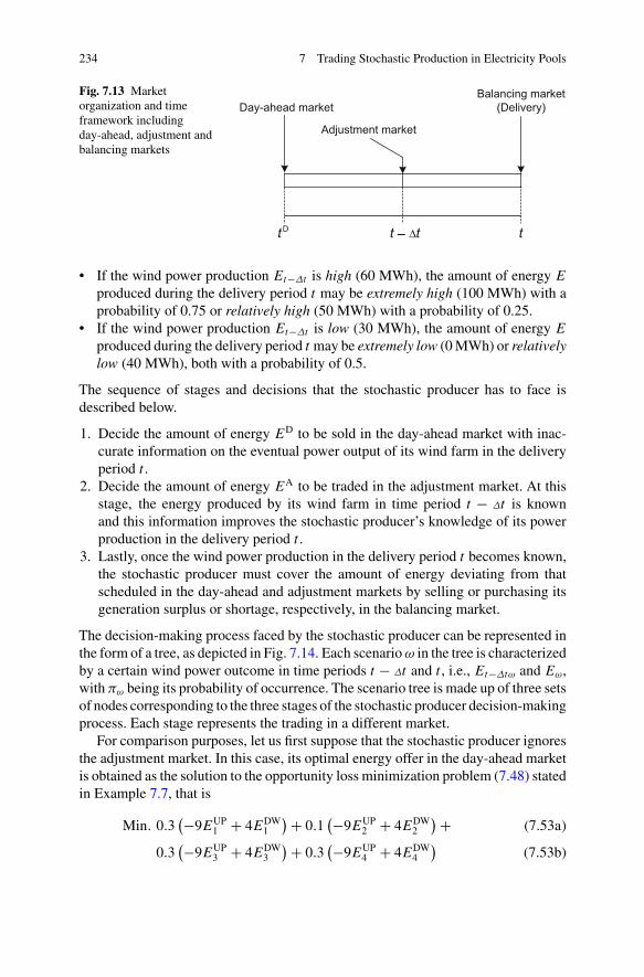
Example 7.9 (Adjustment market) Let us consider a stochastic producer that partic-ipates in an electricity market with the structure and time framework representedin Fig. 7.13. The day-ahead market is cleared at time tD. After the closure of theday-ahead market, bidding in the adjustment market is allowed until Δt time unitsprior to the energy delivery period t . In the balancing market, the energy deviationsincurred by the stochastic producer during the delivery period t are determined withrespect to the dispatch program agreed in the day-ahead and adjustment markets, andpriced accordingly.

Suppose that the day-ahead and adjustment market prices, i.e., �D and�A, are equalto $20/MWh and $19/MWh, respectively. Besides, the imbalance penalties, ψUP

and ψDW, are $9/MWh and $4/MWh in that order, which means that the balancingmarket prices for upward and downward regulation, i.e., �UP and �DW, are given by�UP = �D + ψUP = $29/MWh and �DW = �D − ψDW = $16/MWh.

The stochastic producer owns a 100-MW wind farm whose power output in timeperiod t can be described as follows:

• The amount of energy Et−Δt produced by the wind farm in time period t −Δt maybe high (60 MWh) with a probability of 0.4 or low (30 MWh) with a probabilityof 0.6.


Fig. 7.13 Marketorganization and timeframework includingday-ahead, adjustment andbalancing markets

• If the wind power production Et−Δt is high (60 MWh), the amount of energy E

produced during the delivery period t may be extremely high (100 MWh) with aprobability of 0.75 or relatively high (50 MWh) with a probability of 0.25.

• If the wind power production Et−Δt is low (30 MWh), the amount of energy E

produced during the delivery period t may be extremely low (0 MWh) or relativelylow (40 MWh), both with a probability of 0.5.

The sequence of stages and decisions that the stochastic producer has to face isdescribed below.

1. Decide the amount of energy ED to be sold in the day-ahead market with inac-curate information on the eventual power output of its wind farm in the deliveryperiod t .

2. Decide the amount of energy EA to be traded in the adjustment market. At thisstage, the energy produced by its wind farm in time period t − Δt is knownand this information improves the stochastic producer’s knowledge of its powerproduction in the delivery period t .

3. Lastly, once the wind power production in the delivery period t becomes known,the stochastic producer must cover the amount of energy deviating from thatscheduled in the day-ahead and adjustment markets by selling or purchasing itsgeneration surplus or shortage, respectively, in the balancing market.

The decision-making process faced by the stochastic producer can be represented inthe form of a tree, as depicted in Fig. 7.14. Each scenario ω in the tree is characterizedby a certain wind power outcome in time periods t − Δt and t , i.e., Et−Δtω and Eω,with πω being its probability of occurrence. The scenario tree is made up of three setsof nodes corresponding to the three stages of the stochastic producer decision-makingprocess. Each stage represents the trading in a different market.

For comparison purposes, let us first suppose that the stochastic producer ignoresthe adjustment market. In this case, its optimal energy offer in the day-ahead marketis obtained as the solution to the opportunity loss minimization problem (7.48) statedin Example 7.7, that is

Min. 0.3(−9EUP

1 + 4EDW1

)+ 0.1(−9EUP

2 + 4EDW2

)+ (7.53a)

0.3(−9EUP

3 + 4EDW3

)+ 0.3(−9EUP

4 + 4EDW4

)(7.53b)


Fig. 7.14 Scenario tree describing the three-stage decision-making process faced by the stochasticproducer. The nodes represent points in time where trading decisions are to be made. The branchesrepresent the realization of wind power

s.t. 0 ≤ ED ≤ 150, (7.53c)

100 − ED = EUP1 + EDW

1 , (7.53d)

50 − ED = EUP2 + EDW

2 , (7.53e)


3 , (7.53f)


4 , (7.53g)

EUP1 , EUP

2 , EUP3 , EUP

4 ≤ 0, EDW1 , EDW

2 , EDW3 , EDW

4 ≥ 0, (7.53h)

which yields ED∗ = 40 MWh. The expected opportunity loss (EOL) associated withthis bid is $184. Therefore, the expected profit ρ made by the stochastic producercan be calculated as ρ = �D∑4

ω=1 πωEω −EOL = $20/MWh×47MWh−$184 =$756.

Let us now consider that the stochastic producer trades in the adjustment marketas well. In this case, the best strategy the stochastic producer can adopt is given bythe following expected profit maximization problem,

Max. �DED +

NΩ∑ω=1

πω

(�A

EAω + �UP

EUPω + �DW

EDWω

)(7.54a)

s.t. 0 ≤ ED ≤ E, (7.54b)

0 ≤ ED + EAω ≤ E, ∀ω, (7.54c)

Eω − ED − EAω = EUP

ω + EDWω , ∀ω, (7.54d)

EA1 = EA

2 , EA3 = EA

4 , (7.54e)

EUPω ≤ 0, EDW

ω ≥ 0, ∀ω, (7.54f)


where EAω is the amount of energy sold, if positive, or purchased, if negative, in

the adjustment market by the stochastic producer. The objective function (7.54a)to be maximized is the expected profit, which includes three terms: (i) the profitmade in the day-ahead market, �D

ED; (ii) the expected profit obtained in the ad-justment market, �A∑NΩ

ω=1 πωEAω; and the expected profit made in the balancing

market,∑NΩ

ω=1 πω

(�UP

EUPω + �DW

EDWω

). Note that the last two terms referring to the

adjustment and balancing markets may actually represent a cost in those scenarioswhere the stochastic producer purchases electricity from these markets. Logically,the energy deviations incurred by the stochastic producer are to be computed herewith respect to the forward production program resulting from the day-ahead andadjustment markets, as stated by the set of constraints (7.54d). Equations (7.54e)enforce the nonanticipatory character of the information, which requires the amountof energy traded in the adjustment market be unique irrespective of the wind pro-duction outcome in the future delivery period t . However, the energy offer in theadjustment market may be indeed conditional on the wind power produced in timeperiod t − Δt . In stochastic programming, constraints of the nature of (7.54e) areusually called nonanticipativity constraints.

By replacing parameters in optimization problem (7.54) with their actual values,we end up with the following optimization problem,

Max. 20ED + 0.3(19EA

1 + 29EUP1 + 16EDW

1

)+0.1(19EA

2 + 29EUP2 + 16EDW

2

)+ 0.3(19EA

3 + 29EUP3 + 16EDW

3

)(7.55a)

0.3(19EA

4 + 29EUP4 + 16EDW

4

)s.t. 0 ≤ ED ≤ 100, (7.55b)

0 ≤ ED + EA1 ≤ 100, (7.55c)

0 ≤ ED + EA2 ≤ 100, (7.55d)

0 ≤ ED + EA3 ≤ 100, (7.55e)

0 ≤ ED + EA4 ≤ 100, (7.55f)

100 − ED − EA1 = EUP

1 + EDW1 , (7.55g)

50 − ED − EA2 = EUP

2 + EDW2 , (7.55h)

40 − ED − EA3 = EUP

3 + EDW3 , (7.55i)

0 − ED − EA4 = EUP

4 + EDW4 , (7.55j)

EA1 = EA

2 , EA3 = EA

4 , (7.55k)

EUP1 , EUP

2 , EUP3 , EUP

4 ≤ 0, EDW1 , EDW

2 , EDW3 , EDW

4 ≥ 0, (7.55l)

which results in ED∗ = 100 MWh, EA1

∗ = EA2

∗ = −50 MWh, EA3

∗ = EA4

∗ =−100 MWh, and ρ = $912. This trading strategy, therefore, entails an increase in

7.7 Summary and Conclusions 237

the expected profit equal to $912 − $756 = $156—a 20.64% increment in relativeterms—with respect to the expected profit associated with the offering strategy de-rived from problem (7.53), which ignores the adjustment market. This increase ispartly due to the fact that the future wind power production in the delivery periodt is known with higher accuracy in the adjustment market. Indeed, from the day-ahead market, the stochastic producer foresees a future energy generation in period t

ranging from 0 to 100 MWh. In contrast, from the adjustment market, the stochasticproducer forecasts an energy production varying either from 50 to 100 MWh or from0 to 40 MWh depending on whether the wind energy produced in time period t −Δt ,i.e., Et−Δt , is high (60 MWh) or low (30 MWh). This way, if Et−Δt is high, thestochastic producer purchases 50 MWh in the adjustment market, while if it is low,its energy purchase in this market is increased up to 100 MWh.

In short, the fact that the clearing of the adjustment market is closer in time to theenergy delivery period enhances the profitability of the stochastic producer. Indeed,if the pair of constraints (7.54e) is replaced with the single equation EA

1 = EA2 =

EA3 = EA

4 , in order to disregard this effect, the expected profit made by the stochasticproducer drops to $852, which represents a 6.6% decrease with regard to the expectedprofit resulting from problem (7.54).

In reality, the electricity prices in the day-ahead and adjustment markets are alsouncertain. Furthermore, since the trading volume in adjustments markets is generallylower than in the day-ahead market, the electricity price in adjustment markets isoften more volatile. As a result, the stochastic producer must face a tradeoff betweenselling in the day-ahead market at less volatile prices and trading in the adjustmentmarket with a reduced level of uncertainty about its future energy production. Thistradeoff can be resolved by means of the stochastic programming solution approachpresented in this section.

7.7 Summary and Conclusions

Renewable energy producers are increasingly required to participate in electricitymarkets under the same rules as conventional power producers. However, the com-petitive sale of renewable energy by stochastic producers is cursed with the weatherdependency of the underlying energy source, e.g., sunlight or wind. Stochastic pro-ducers are thus forced to channel part of their business into the balancing market,where they can take part with perfect knowledge of their production.

Compared to the electricity prices in markets with early gate closures, such as day-ahead and adjustment markets, balancing market prices are generally less predictableand/or less competitive. Consequently, as the stochastic producer becomes more andmore dependent on the balancing market, its profitability may rapidly deteriorate.Therefore, the stochastic producer must smartly decide its involvement in day-ahead,adjustment, and balancing markets according to its best guess on market prices andfuture power production.


The trading problem of a stochastic producer is described in this chapter as amulti-stage decision-making problem under uncertainty. We identify the assump-tions that render this problem analytically solvable and provide the correspondingexact solutions. For those cases in which these assumptions prove to be unrealistic,simplistic or too constraining, a more general modeling approach based on stochasticprogramming and the concept of scenarios is introduced to determine the best tradingstrategy for the stochastic producer.

7.8 Further Reading

For a basic introduction to statistical decision theory, the reader is referred to [14].From the same author, [15] offers a more complete treatment of the subject, includingthe newsvendor problem, which is the general formulation of the power tradingproblem.

Further reading on analytical results on the trading problem for stochastic powerproducers consists mainly of research articles focusing on the case of wind powerproducers. The optimal strategy based on the offer of a quantile of the wind powerdistribution is proposed and tested in [4; 12; 17]. Further analytical results includingand extending part of the results presented in this chapter can be found in [3; 6].Finally, [8] provides a general discussion, including an application to electricitymarkets, on the relationship between loss functions and the optimal forecasts.

On the other hand, the short-term trading problem of a wind power producer istackled in [10; 11; 13] using stochastic programming. Reference [5] also describes anumber of trading models for retailers, consumers and producers (including nondis-patchable agents) that are built upon stochastic programming, and provides insightinto risk management and the scenario-based modeling of the uncertainties affectingtrading decisions.

The trading problem for price-maker producers employing renewable sourceswith variable and stochastic nature is considered in [2; 18], making use of stochasticMathematical Programs with Equilibrium Constraints.

Exercises

7.1 A forecaster predicts that the energy production E of a wind farm during a giventrading period t is characterized by the following probability density function pE( · ):

pE(E) =

⎧⎪⎪⎪⎪⎪⎨⎪⎪⎪⎪⎪⎩

E − 100

625, 100 ≤ E < 125,

150 − E

625, 125 ≤ E < 150,

0, elsewhere.

(7.56)

7.8 Further Reading 239

1. Determine the cumulative distribution function FE( ·) for wind power production.2. Assume that the imbalance penalties in a two-price market are ψUP = $9 /MWh

and ψDW = $4/MWh. Determine the optimal offer and the resulting expectationof the imbalance cost.

3. Now determine the optimal offer and the resulting expectation of the imbalancecost assuming that the imbalance penalties are ψUP = $4/MWh and ψDW =$9/MWh.

7.2 Consider the definition of u in Example 7.2. Let us assume that the probabilitydensity function for u is

pu(u) =

⎧⎪⎪⎪⎪⎨⎪⎪⎪⎪⎩

u + 20

625, −20 ≤ u < 5,

30 − u

625, 5 ≤ u < 30,

0, elsewhere.

(7.57)

1. Determine the expected value of the balancing price in a one-price market. If theforecast for wind power production is the same as in Exercise 7.1, what is theoptimal offer?

2. Determine the expected values of the imbalance penalties ψUP and ψDW in atwo-price market. If the forecast for wind power production is the same as inExercise 7.1, what is the optimal offer?

7.3 In a two-price market, the expectation of the imbalance penalties, conditional onthe day-ahead price, is given by the following.

E{ψUP|�D} =10 − 1

10�D, (7.58)

E{ψDW|�D} =1

8�D

. (7.59)

Let us consider a uniform distribution for the stochastic production with lower andupper bounds equal to 100 MWh and 150 MWh, respectively. Determine the optimaloffering curve, assuming that the day-ahead price is nonnegative and can take valuesup to $100/MWh.

7.4 Consider the distribution of wind power production in Exercise 7.1, and the deter-ministic penalties ψUP = $9/MWh and ψDW = $4/MWh. Determine the risk-aversebid with parameter α = 0.2. Assuming a day-ahead price �D = $50/MWh, deter-mine the expected value of the profit, the value at risk (VaR5%) and the conditionalvalue at risk (CVaR5%) of the profit.

7.5 Suppose that the energy production of a certain wind farm in a given tradingperiod t can be modeled by a uniform distribution between 0 MWh and 50 MWh.

1. Construct a set of four equiprobable and uniformly spaced scenarios thatapproximates this uniform distribution.

2. Based on this scenario set and knowing that the imbalance penalties, ψUP andψDW, are deterministic and equal to $3/MWh and $6/MWh, respectively, for-


mulate and solve a stochastic programming model to calculate the energy offerin the day-ahead market that minimizes the expected imbalance cost of the windfarm.

7.6 Reformulate the stochastic programming model of the previous exercise toaccount for the risk aversion of the wind power producer using the ConditionalValue-at-Risk of its profit distribution at a confidence level of 99%. Then, obtain theoptimal bid of the wind power producer in the day-ahead market as a function of arisk-aversion parameter and draw the resulting efficient frontier.

7.7 Consider a solar power producer that participates in an electricity market withthe structure and time framework depicted in Fig. 7.13 of Example 7.9. The solarproducer owns a 50-MW photovoltaic power plant whose energy output in timeperiod t is stochastic and can be described as follows:

• The amount of energy Et−Δt produced by the solar power plant in time periodt − Δt may be high (45 MWh) with a probability of 0.7 or low (5 MWh) with aprobability of 0.3.

• If the solar power production Et−Δt is high (45 MWh), the amount of energy E

produced during the delivery period t may be extremely high (50 MWh) with aprobability of 0.35 or relatively high (41 MWh) with a probability of 0.65.

• If the solar power production Et−Δt is low (5 MWh), the amount of energy E

produced during the delivery period t may be extremely low (0 MWh) with aprobability of 0.70 or relatively low (10 MWh) with a probability of 0.30.

Furthermore, the day-ahead and adjustment market prices, i.e., �D and �A, are knownto be equal to $45/MWh and $46/MWh, respectively, and the imbalance penalties,ψUP and ψDW, equal to $10/MWh and $8/MWh, in that order.

1. Construct a scenario tree similar to that in Fig. 7.14 of Example 7.9 to describethe decision-making process faced by the solar power producer.

2. Compute the optimal bid of the solar power producer in the day-ahead market ifthe adjustment market is disregarded.

3. Compute the optimal bid of the solar power producer in the day-ahead market ifthe adjustment market is taken into account and calculate how much the expectedprofit of the solar power producer increases with respect to the previous case.Determine also how much of this increase is due to the fact that the future energyproduction of the photovoltaic power plant in period t is known with higheraccuracy in the adjustment market than in the day-ahead market.

7.8 Consider a 60-MW solar power plant whose power output in a given tradingperiod t can be either 35 and 60 MW, with probabilities 0.6 and 0.4, respectively. Itis known that:

• The price in the day-ahead market for period t can be either $25/MWh or$50/MWh, with probabilities 0.3 and 0.7, in that order.

• If the day-ahead market price is equal to $25/MWh, the imbalance penal-ties for upward and downward balancing energy are $10 /MWh and $2/MWh,respectively.

References 241

• In contrast, if the day-ahead market price is equal to $50/MWh, these imbalancepenalties take on the values $5/MWh and $4/MWh instead.

Use the information about offering curves provided in Sect. 8.4 of Chap. 8 (see, inparticular, Example 8.9 in this chapter) to formulate and solve a stochastic program-ming model that computes, as an increasing function of the day-ahead electricityprice, the optimal energy offer in the day-ahead market that maximizes the expectedprofit of the solar power producer.

Based on the comments and explanations in Sect. 7.4.2, justify the obtainedsolution.

7.9 Repeat Exercise 7.8 for the case that:

• If the day-ahead market price is $25/MWh, the imbalance penalties for upwardand downward balancing energy are $5 /MWh and $4/MWh, respectively.

• If the day-ahead market price is equal to $50/MWh, the imbalance penalties are$10/MWh and $2/MWh instead.

7.10 Try to solve Exercises 7.8 and 7.9 analytically. Can both problems be solvedthis way? If not, motivate why.

References

1. Artzner, P., Delbaen, F., Eber, J.M., Heath, D.: Coherent measures of risk. Math. Financ. 9(3),203–228 (1999)

2. Baringo, L., Conejo, A.J.: Strategic offering for a wind power producer. IEEE Trans. PowerSyst. (2013). In press

3. Bitar, E., Rajagopal, R., Khargonekar, P., Poolla, K., Varaiya, P.: Bringing wind energy tomarket. IEEE Trans. Power Syst. 27(3), 1225–1235 (2012)

4. Bremnes, J.B.: Probabilistic wind power forecasts using local quantile regression. Wind Energy7(1), 47–54 (2004)

5. Conejo, A.J., Carrión, M., Morales, J.: Decision Making Under Uncertainty in ElectricityMarkets. International Series in Operations Research & Management Science. Springer, NewYork (2010)

6. Dent, C., Bialek, J.W., Hobbs, B.F.: Opportunity cost bidding by wind generators in forwardmarkets: Analytical results. IEEE Trans. Power Syst. 26(3), 1600–1608 (2011)

7. Gabriel, S.A., Conejo, A.J., Fuller, J.D., Hobbs, B.F., Ruiz, C.: Complementarity Modeling inEnergy Markets. International Series in Operations Research & Management Science. Springer,New York (2013)

8. Gneiting, T.: Quantiles as optimal point forecasts. Int. J. Forecast. 27(2), 197–207 (2011)9. Kaplan, W.: Advanced Calculus, 5th edn., chap. 4, pp. 253–257. Addison-Wesley Higher

Mathematics. Addison-Wesley, Reading, MA (2002)10. Matevosyan, J., Söder, L.: Minimization of imbalance cost trading wind power on the short-

term power market. IEEE Trans. Power Syst. 21(3), 1396–1404 (2006)11. Morales, J.M., Conejo, A.J., Pérez-Ruiz, J.: Short-term trading for a wind power producer.

IEEE Trans. Power Syst. 25(1), 554–564 (2010)12. Pinson, P., Chevalier, C., Kariniotakis, G.: Trading wind generation from short-term

probabilistic forecasts of wind power. IEEE Trans. Power Syst. 22(3), 1148–1156 (2007)13. Rahimiyan, M., Morales, J.M., Conejo, A.J.: Evaluating alternative offering strategies for wind

producers in a pool. Appl. Energy 88(12), 4918–4926 (2011)


14. Raiffa, H.: Decision Analysis: Introductory Lectures on Choices Under Uncertainty. Addison-Wesley, Reading, MA (1968)

15. Raiffa, H., Schlaifer, R.: Applied Statistical Decision Theory. Division of Research – HarvardBusiness school, Boston, MA (1964)

16. Rockafellar, R.T., Uryasev, S.: Optimization of Conditional Value-at-Risk. J. Risk 2, 21–41(2000)

17. Zugno, M., Jónsson, T., Pinson, P.: Trading wind energy on the basis of probabilistic forecastsboth of wind generation and of market quantities. Wind Energy 16, 909–926 (2012).

18. Zugno, M., Morales, J.M., Pinson, P., Madsen, H.: Pool strategy of a price-maker wind powerproducer. IEEE Trans. Power Syst. 28(3), 3440–3450 (2013)

chapter 7 trading stochastic production in electricity...

Documents