chapter 7 regularization for deep...
TRANSCRIPT

=1truein =1truein
Peng et al.: Deep Learning and Practice 1'
&
$
%
Chapter 7
Regularization for Deep Learning
Spring 2017 A
1896
E S
NCTU CS

Peng et al.: Deep Learning and Practice 2'
&
$
%
Regularization
• In machine learning, we optimize a cost function defined w.r.t. the
training set
J(θ) = Ex,y∼pdataL(f(x; θ), y)
where
– L is the per-example loss function
– f(x; θ) is the model prediction,
– y is the target output
– pdata is the empirical distribution
• We however hope that doing so will minimize the expected loss over
the true data-generating distribution pdata(x, y)
J∗(θ) = Ex,y∼pdataL(f(x; θ), y)
Spring 2017 A
1896
E S
NCTU CS

Peng et al.: Deep Learning and Practice 3'
&
$
%
• If we knew the true distribution pdata(x, y), minimizing J∗(θ) would
become a pure optimization problem; but, when we do not know the
true distribution but only the empirical distribution pdata(x, y) over the
training data, we have a machine learning problem
• One central problem in machine learning is how to make an algorithm
work well not just only on training data, but also on new inputs
• Strategies used to reduce test error, possibly at the expense of
increased training error, are known collectively as regularization
Spring 2017 A
1896
E S
NCTU CS

Peng et al.: Deep Learning and Practice 4'
&
$
%
Revisiting Capacity, Underfitting and Overfitting
• To characterize analytically the relationship between a model’s capacity
and the phenomena of underfitting and overfitting when it is trained
using the maximum likelihood
• Example: Linear Regression
x Rep. φ(x) Model y -
y
‖y − y‖2
• To predict y from x, we construct a model of the form
y(x) = f(x; w) = wT φ(x)
and make a point estimate of the parameters w by minimizing
Ex,y∼pdata‖y − y(x)‖2
Spring 2017 A
1896
E S
NCTU CS

Peng et al.: Deep Learning and Practice 5'
&
$
%
• This is equivalent to maximizing the expected likelihood function
Ex,y∼pdatap(y|x) by assuming the following data model
p(y|x) = N (y; y(x), σ2)
• The optimal prediction which achieves the minimum expected
(squared) generalization error
g∗(x) = arg ming(∙)
Ex,y∼pdata‖y − g(x)‖2
is given by the conditional mean
g∗(x) = Ey∼pdata(y|x)[y]
• The expected generalization error of the model y(x) is then seen as
the sum of Bayes error and the expected error between the optimal and
the model predictions
Spring 2017 A
1896
E S
NCTU CS

Peng et al.: Deep Learning and Practice 6'
&
$
%
Ex,y∼pdata‖y − y(x)‖2
= Ex,y∼pdata‖y − g∗(x) + g∗(x) − y(x)‖2
= Ex,y∼pdata‖y − g∗(x)‖2
︸ ︷︷ ︸Bayes error
+Ex∼pdata‖g∗(x) − y(x)‖2
where the cross-term
Ex,y∼pdata[2(y − g∗(x))(g∗(x) − y(x)]
= Ex∼pdata(x)Ey∼pdata(y|x)[2(y − g∗(x))(g∗(x) − y(x)]
= Ex∼pdata(x)[2���
������
���:Ey∼pdata(y|x)[(y − g∗(x))](g∗(x) − y(x))]
= 0
• The Bayes error, which arises from the intrinsic noise on data,
represents the minimum achievable value of the expected
generalization error, and is independent of y(x) and training data
Spring 2017 A
1896
E S
NCTU CS

Peng et al.: Deep Learning and Practice 7'
&
$
%
• On the other hand, the expected error between the optimal and the
model predictions has to do with training data because y(x) is
obtained by making a point estimate of w based on a particular
training data set D = {X(train), y(train)}
Ex∼pdata‖g∗(x) − y(x)‖2
• Assume we are concerned with how the model performs over an
ensemble of training data sets, and denote the model y(x) trained with
a particular data set D as y(x;D)
• For a given x, we then evaluate the expected error between the optimal
and model predictions w.r.t. the distribution of training data to be
ED‖g∗(x) − y(x;D)‖2
= ED‖g∗(x) − ED(y(x;D)) + ED(y(x;D)) − y(x;D)‖2
= ‖g∗(x) − ED(y(x;D))‖2
︸ ︷︷ ︸(bias)2
+ ED‖ED(y(x;D)) − y(x;D)‖2
︸ ︷︷ ︸variance
Spring 2017 A
1896
E S
NCTU CS

Peng et al.: Deep Learning and Practice 8'
&
$
%
where the cross-term is again computed to be zero
• The (bias)2 represents the extent to which the average model
prediction over all training data sets differs from the optimal prediction
• The variance measures the extent to which the model y(x;D) is
sensitive to the particular choice of training set
• Both terms can be further averaged over different x’s to obtain the
expected generalization error of the model y(x)
Bayes error + Ex∼pdata[(bias)2] + Ex∼pdata
[variance]
Spring 2017 A
1896
E S
NCTU CS

Peng et al.: Deep Learning and Practice 9'
&
$
%
Fitting Sinusoidal Functions
• Setting
– Data: y = sin(2πx) + ε, p(ε) = N (ε; 0, σ2)
– Model: y = wT φ(x), φ(x) is Gaussian basis
– 100 training data sets, each having 25 data points (x, y)
• Training
min Ex,y∼pdata‖y − y(x)‖2 + λwT w
Spring 2017 A
1896
E S
NCTU CS

Peng et al.: Deep Learning and Practice 10'
&
$
%
Left: y(x;D) with different training sets
Right: g∗(x) = sin(2πx) (Green); ED[y(x;D)] (Red)
Spring 2017 A
1896
E S
NCTU CS

Peng et al.: Deep Learning and Practice 11'
&
$
%
Trading off Bias and Variance
In general, models of high capacity have low bias and high variance,
whereas models of low capacity have high bias and low variance
Spring 2017 A
1896
E S
NCTU CS

Peng et al.: Deep Learning and Practice 12'
&
$
%
Parameter Norm Penalties
• Limiting the model capacity by adding a norm penalty Ω(θ)
J(θ; X, y) = J(θ; X, y) + αΩ(θ)
where X, y are training data and α ∈ [0,∞) weights the relative
contribution of the norm penalty to the objective function
• Generally, for neural networks, only the weights w of the affine
transformation wT x + b are penalized, with the bias b often left
unregularized
• This is because regularizing the bias can introduce a significant
amount of underfitting, e.g., in the linear regression problem
• Hereafter we denote as w weights that should be regularized and as θ
all the parameters {w, b}
Spring 2017 A
1896
E S
NCTU CS

Peng et al.: Deep Learning and Practice 13'
&
$
%
L2 Regularization
• The L2 parameter regularization drives the weights closer to the origin
by adding a L2-norm penalty Ω(θ) = 12‖w‖2
2 (i.e. weight decay)
J(w; X, y) = J(w; X, y) +α
2wT w
• The gradient of J(w; X, y) w.r.t. w is
∇wJ(w; X, y) = ∇wJ(w; X, y) + αw
• To gain insight into the behavior of weight decay, we make a quadratic
approximation to J around w∗ = arg minw J(w)
J(w) = J(w∗) +12(w − w∗)T H(w − w∗)
where H is the Hessian matrix of J evaluated at w∗
• We then solve for the minimum of J(w; X, y) by substituting J for J
Spring 2017 A
1896
E S
NCTU CS

Peng et al.: Deep Learning and Practice 14'
&
$
%
and setting to zero its gradient w.r.t. w
∇wJ(w; X, y) ≈ H(w − w∗) + αw = 0
• The regularized solution w is given by
w = (H + αI)−1Hw∗
• Going further, we know that H must have the factorization
H = QΛQT
because the Hessian matrix is real and symmetric, and is positive
semi-definitive when evaluated at w∗
• We then have
w = (QΛQT + αI)−1QΛQT w∗
= (Q(Λ + αI)QT )−1QΛQT w∗
Spring 2017 A
1896
E S
NCTU CS

Peng et al.: Deep Learning and Practice 15'
&
$
%
= Q (Λ + αI)−1Λ︸ ︷︷ ︸
QT w∗
• From the above, the component of w that is aligned with the i-th
eigenvector is re-scaled by λi
λi+α
• Recall that
J(w; X, y)
≈ J(w∗) +12(w − w∗)T H(w − w∗)
= J(w∗) +12(w − w∗)T QΛQT (w − w∗)
where along directions corresponding to large λi, a further deviation
from w∗ contributes significantly to increasing the objective function
• The effect of L2 regularization is to decay away components of w∗
along unimportant directions with λi � α
Spring 2017 A
1896
E S
NCTU CS
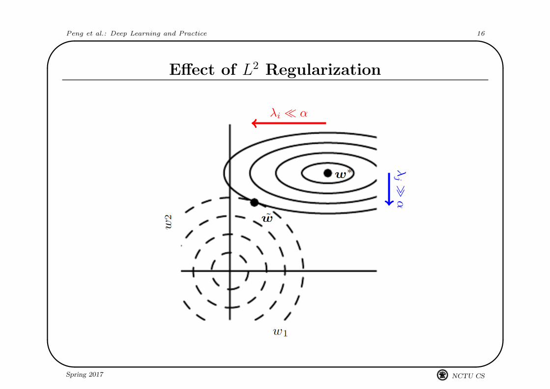
Peng et al.: Deep Learning and Practice 16'
&
$
%
Effect of L2 Regularization
λi � α
λj�
α
Spring 2017 A
1896
E S
NCTU CS

Peng et al.: Deep Learning and Practice 17'
&
$
%
L1 Regularization
• Another popular parameter norm regularization is to add a L1-norm
penalty Ω(θ) = ‖w‖1 =∑
|wi|
J(w; X, y) = J(w; X, y) + α‖w‖1
• As with L2 regularization, we hope to analyze the effect of L1
regularization by making a quadratic approximation to J at w∗
J(w; X, y) ≈ J(w∗) +12(w − w∗)T H(w − w∗) + α‖w‖1
• It is however noticed that the full general Hessian does not admit a
clean algebraic solution to the following problem
∇wJ(w; X, y) ≈ H(w − w∗) + αsign(w) = 0
Spring 2017 A
1896
E S
NCTU CS

Peng et al.: Deep Learning and Practice 18'
&
$
%
• We then make a further assumption that H is diagonal
H =
H1,1 0 ∙ ∙ ∙ 0
0 H2,2 ∙ ∙ ∙ 0...
.... . .
...
0 0 ∙ ∙ ∙ Hn,n
to arrive at
J(w; X, y) ≈ J(w∗) +∑
i
[12Hi,i(wi − w∗
i )2 + α|wi|
]
• Without loss of generality, let us assume w∗i > 0; it can then be seen
that the optimal wi which minimizes J lies in [0, w∗i ]
Spring 2017 A
1896
E S
NCTU CS

Peng et al.: Deep Learning and Practice 19'
&
$
%
α|wi|
12Hi,i(wi − w∗
i )2
12Hi,i(wi − w∗
i )2 + α|wi|
w∗i
wi
−2 2 4 6
2
4
6
wi
J
Spring 2017 A
1896
E S
NCTU CS

Peng et al.: Deep Learning and Practice 20'
&
$
%
• Setting to zero the partial derivative of J w.r.t. wi yeilds
wi = w∗i −
α
Hi,i
• The regularized solution is then given by
wi =
w∗i − α
Hi,iif w∗
i ≥ αHi,i
0 otherwise
• It is seen that L1 regularization results in a solution that is more sparse
(i.e. having more zero weights); a similar result occurs when w∗i < 0
• In contrast, L2 regularization in the present case does NOT cause the
parameters to become sparse
wi =Hi,i
Hi,i + αw∗
i ,
• Least absolute shrinkage and selection operator (LASSO): a
Spring 2017 A
1896
E S
NCTU CS

Peng et al.: Deep Learning and Practice 21'
&
$
%
feature selection mechanism based on L1 penalty + linear model +
least-squares cost
−1 1 2
−1
1
2
w1
w2L1 regularization
L2 regularization
Spring 2017 A
1896
E S
NCTU CS
Peng et al.: Deep Learning and Practice 22'
&
$
%
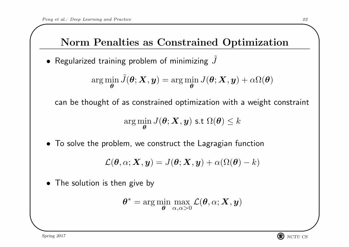
Norm Penalties as Constrained Optimization
• Regularized training problem of minimizing J
arg minθ
J(θ; X, y) = arg minθ
J(θ; X, y) + αΩ(θ)
can be thought of as constrained optimization with a weight constraint
arg minθ
J(θ; X, y) s.t Ω(θ) ≤ k
• To solve the problem, we construct the Lagragian function
L(θ, α; X, y) = J(θ; X, y) + α(Ω(θ) − k)
• The solution is then give by
θ∗ = arg minθ
maxα,α>0
L(θ, α; X, y)
Spring 2017 A
1896
E S
NCTU CS

Peng et al.: Deep Learning and Practice 23'
&
$
%
• When α is fixed at its optimal value α∗, θ is found by minimizing
J(θ; X, y) + α∗Ω(θ),
which has exactly the same form as J
• The optimal solution θ∗ must satisfy (see the next two slides)
∇θJ(θ∗; X, y) = −α∗∇θΩ(θ∗)
• Note that the value of α∗ does not directly tell us the value of k
• Some use explicit constraints rather than penalties
1. Take a step downhill on J(θ)
2. Project θ back to the set {θ : Ω(θ) < k}
(Repeat steps 1 and 2 until some stopping criterion is satisfied)
Spring 2017 A
1896
E S
NCTU CS

Peng et al.: Deep Learning and Practice 24'
&
$
%
Trajectory of L2 Regularization
1 2
1
2
w1
w2
Spring 2017 A
1896
E S
NCTU CS

Peng et al.: Deep Learning and Practice 25'
&
$
%
Trajectory of L1 Regularization
1 2
1
2
w1
w2
Spring 2017 A
1896
E S
NCTU CS

Peng et al.: Deep Learning and Practice 26'
&
$
%
Early Stopping
• One effective way of determining when the training process should stop
1. Run training for n steps
2. Check validation error
3. Store model parameters if validation error reduces
4. Repeat 1-3 until validation error does not improve after a few trials
5. Return model parameters
Spring 2017 A
1896
E S
NCTU CS

Peng et al.: Deep Learning and Practice 27'
&
$
%
Early Stopping as Regularization
• In a sense, early stopping restricts the training to a small volume of
parameter space around the initial w0
• The reachable volume is determined by the product τε of the training
iterations τ and learning rate ε
• The product τε plays a similar role to α−1 in L2 regularization
arg minw
J(w; X, y) +α
2wT w,
which is equivalent to
minw
J(w; X, y) s.t. wT w ≤ kα
(Check Section 7.8 for an approximate analysis)
• Early stopping however has the advantage of automatically determining
the correct amount of regularization (i.e. the value of τε ≈ α−1)
Spring 2017 A
1896
E S
NCTU CS

Peng et al.: Deep Learning and Practice 28'
&
$
%
Bootstrap Aggregating (Bagging)
• Idea: To train several models separately and have them vote on the
output for test examples (a.k.a. model averaging or ensemble methods)
• Suppose that each model makes a random error εi on each example
with mean zero, E[ε2i ] = v, and E[εiεj ] = c
• Then, the error made by the average prediction of all k models is
E
(1k
∑
i
εi
)2
=1k2
E
∑
i
ε2i +∑
j 6=i
εiεj
=1k
v +k − 1
kc
• When errors are highly correlated, i.e. E[εiεj ] = c = v, the mean
squared error reduces to v; the model averaging does not help
• When they are uncorrelated, the mean squared error is reduced by a
factor of 1/k
Spring 2017 A
1896
E S
NCTU CS

Peng et al.: Deep Learning and Practice 29'
&
$
%
• In other words, on average, the ensemble will perform at least as well
as any of its members, and significantly better if the members make
independent errors
Cartoon depiction of bagging
Spring 2017 A
1896
E S
NCTU CS

Peng et al.: Deep Learning and Practice 30'
&
$
%
Dropout
• Idea: To train a bagged ensemble of exponentially many neural
networks that consist of all subnetworks of a base network
Spring 2017 A
1896
E S
NCTU CS

Peng et al.: Deep Learning and Practice 31'
&
$
%
• Subnetwork construction: To remove nonoutput units through
multiplication of their output values by zero, with a mask vector μ
indicating which units to keep
Spring 2017 A
1896
E S
NCTU CS

Peng et al.: Deep Learning and Practice 32'
&
$
%
• Typically, an input unit is included with probability 0.8 and a hidden
unit with probability 0.5
• Dropout training: In each mini-batch step, we randomly sample a
binary mask μ; run forward- and back-propagation; and update
parameters as usual
• This amounts to minimizing
EμJ(θ, μ),
with each subnetwork inheriting a different subset of parameters from
the parent neural network (i.e. subnetworks share parameters)
• Ensemble inference: To accumulate votes from all the subnetworks
p(y|x) =∑
μ
p(u)p(y|x, μ) = Eμp(y|x, μ),
where p(u) is the distribution used to sample μ at training time
• The summation over μ involves an exponential number of terms, and
Spring 2017 A
1896
E S
NCTU CS

Peng et al.: Deep Learning and Practice 33'
&
$
%
is thus practically intractable
• One workaround is to approximate the inference with sampling
p(y|x) = Eμp(y|x, μ) ≈1N
N∑
i=1
p(y|x, μ(i))
• Another empirical approach, termed the weight scaling inference
rule, allows us to approximate p(y|x) in one model: the model with all
units, but with the weights going out of unit i multiplied by the
probability of including unit i
• The motivation is to capture the right expected value of output from
that unit, or to make sure that the expected total input to a unit at
test time is roughly the same as that at training time
• The weight scaling inference rule is exact in some settings, e.g. deep
networks that have hidden layers without non-linearities
Spring 2017 A
1896
E S
NCTU CS

Peng et al.: Deep Learning and Practice 34'
&
$
%
• As an example, it is shown empirically that, in the present context,
p(y|x) = Eμp(y|x, μ) ≈ c × 2d
√∏
i
p(y|x, u(i))
where c is for normalization and 2d is the number of all possible u’s
• For a softmax regression classifier with input x and dropout, we have
p(y|x; u) = softmax(W T (u � x) + b
)y,
with each element ui having an equal probability of being 0 or 1
• By an application of the geometric mean approximation, we obtain an
ensemble softmax classifier with
p(y|x) ∝ exp
(12W T
y,:︸ ︷︷ ︸
x + by
)
(Check Section 7.12 for details)
Spring 2017 A
1896
E S
NCTU CS

Peng et al.: Deep Learning and Practice 35'
&
$
%
Pros and Cons
• Values of dropout go beyond bagging, e.g. removal of hidden units is
similar to adaptive destruction of high-level contents
• Shared hidden units learn features useful in many contexts/subnetworks
• Applicable to many types of models
• More effective than other standard regularizers
• Computationally cheap O(n) for training and storage
• Increased model size needed for more capable subnetworks
• Less effective with few labeled training examples
• etc.
Spring 2017 A
1896
E S
NCTU CS

Peng et al.: Deep Learning and Practice 36'
&
$
%
Multitask Learning
• Idea: To improve generalization by pooling examples for several tasks
Shared parameters
Task specific parameters
Unsupervised Task
Supervised Tasks
• Assumption: there exists a common pool of factors that explain the
data variations, while each task is linked to a subset of these factors
• The cost function may involve both supervised and unsupervised parts
Spring 2017 A
1896
E S
NCTU CS

Peng et al.: Deep Learning and Practice 37'
&
$
%
Data Augmentation
• Idea: To add fake data to make the model generalize better
• Effective for some specific tasks, e.g. image recognition
– Translation, rotation, scaling, etc. of training images
– Noise injection in inputs, hidden units, outputs, and weights
• Not as readily applicable to many other tasks, e.g. density estimation
Spring 2017 A
1896
E S
NCTU CS

Peng et al.: Deep Learning and Practice 38'
&
$
%
Adversarial Training
• Idea: To encourage the model y(x) to be locally constant in the
vicinity of training data x by including adversarial examples for training
x′ → x, y(x′) → y(x)
• This can be easily violated with simple linear models y(x) = wT x
|y(x + ε) − y(x)| ≤ |w|T |ε| ≈ ‖w‖1c, with |εi| = c
• Adversarial examples
Spring 2017 A
1896
E S
NCTU CS

Peng et al.: Deep Learning and Practice 39'
&
$
%
Review
• Regularization as variance and bias trade-off
• Parameter norm penalties: L2 and L1 regularization
• Early stopping
• Bagging
• Dropout
• Multitask learning
• Data augmentation
• Adversarial training
• etc.
Spring 2017 A
1896
E S
NCTU CS