chapter 7 probability and statistics - utah education · pdf filechapter 7 probability and...

Chapter 7Probability and Statistics

In this chapter, students develop an understanding of data sampling and making inferences from representationsof the sample data, with attention to both measures of central tendency and variability. They will do this bygathering samples, creating plots, representing the data in a variety of ways and by comparing sample data sets,building on the familiarity with the basic statistics of data sampling developed over previous years. They findprobabilities, including those for compound events, using organized lists, tables, and tree diagrams to display andanalyze compound events to determine their probabilities. Activities are designed to help students move fromexperiences to general conjectures about probability and number. They compare graphic representations of datafrom di↵erent populations to make comparisons of center and spread of the populations, through both calculationsand observation.

Statistics begins in the middle of the nineteenth century during the Crimean War, when Florence Nightingale (anurse with the British Army) began to notice the excess of British soldiers dying in the hospital of “complicationsfrom their injuries” but not from the injuries themselves. Nurse Nightingale suspected that this could be attributedto the sterile (lack thereof) conditions of the field hospitals, and not to the nature of the injuries themselves. Shebegan to gather data, both from field hospitals that attempted to maintain sanitary conditions and those that didnot. Her goal was not just to uncover causes, but to suggest remedies that can be implemented instantly. Shestudied the data, correlating hospital practices with patient mortality, and concluded that there was one rule that, ifapplied faithfully, would significantly change the result: physicians should wash their hands. When she presentedthis suggestion to the high command, the response did not meet the urgency she felt. So, she appealed to QueenVictoria: she invented bar graphs to present these data so that the Queen could visualize the significance of hersuggestion. It worked: the Queen issued an order that physicians should wash their hands, and that was thebeginning of scientific statistics and modern medical practice.

Probability and Statistics are intricately entwined, but historically, the origins are quite distinct. Probability ques-tions arise naturally in games of chance, and over the centuries gamblers placed their faith (and money) on rulesthat, with or without any foundation, had become folklore. Recall from Chapter 1 that, n the mid-seventeenthcentury, the Chevalier de Mere asked the mathematician Blaise Pascal about a rule in a game of dice that, un-fortunately, did not work for him. Pascal began a correspondence with Pierre Fermat (two of the leading math-ematicians of the century), and between them a theory of probabilities developed that accounted for de Mere’smisfortune.Today that theory is fundamental in the study of many processes, particularly biological and economicones, where there is the possibility of random influences on the sequence of events.

Section 1 begins with an exploration of basic probability and notation, using objects such as dice and cards.Students will develop modeling strategies to make sense of di↵erent contexts and then move to generalizations.In order to perform the necessary probability calculations, students work with fraction and decimal equivalents.These exercises should strengthen students’ abilities with rational number operations. Some probabilities are notknown, but can be estimated by repeating a trial many times, thus estimating the probability from a large numberof trials. This is known as the Law of Large Numbers, and will be explored by tossing a Hershey’s Kiss manytimes and calculating the proportion of times the Kiss lands on its base.

7MF7-1 ©2014 University of Utah Middle School Math Project in partnership with theUtah State O�ce of Education. Licensed under Creative Commons, cc-by.

Section 2 investigates the basics of gathering samples randomly in order to learn about characteristics of popu-lations, in other words, the basics of inferential statistics. Typically, population values are not knowable becausemost populations are too large and their characteristics too di�cult to measure. “Inferential statistics” means thatsamples from the population are collected, and then analyzed in order to make judgments about the population.The key to obtaining samples that represent the population is to select samples randomly. This is not always easyto do, and an important part of this chapter is to think about what “random sample” means. Students will gathersamples from real and pretend populations, plot the data, perform calculations on the sample results, and then usethe information from the samples to make decisions about characteristics of the population.

Section 3 uses inferential statistics to compare two or more populations. In this section, students use data fromexisting samples and also gather their own data. They compare plots from the di↵erent populations, and then makecomparisons of center and spread of the populations, through both calculations and visual comparisons.

This unit introduces the importance of fairness in random sampling, and of using samples to draw inferencesabout populations. Some of the statistical tools used in Grade 6 will be practiced and expanded upon as studentscontinue to work with measures of center and spread to make comparisons between populations. Students willinvestigate chance processes as they develop, use, and evaluate probability models. Compound events will beexplored through simulation, and by multiple representations such as tables, lists, and tree diagrams.

The eighth grade statistics curriculum will focus on scatter plots of bivariate measurement data. Bivariate dataare also explored in Secondary Math I. However, statistics standards in Secondary Math I, II, and III return toexploration of center and spread, random probability calculations, sampling and inference.

The student workbook begins with the anchor problem: the game “Teacher always wins!” The purpose of thisparticular activity is to start thinking about what kind of data are needed to resolve a problem (in this case, theapparent unfairness of the game), and secondarily, to illustrate that such resolution is not always as simple as itoriginally seems. This point is made again towards the end of the first section with the Monty Hall problem. In themeantime, the problem introduces the student to all of the fundamental ideas of this chapter. In order to illustratethese goals, as will be done in the succeeding sections, let’s first look at this type of problem in the context ofsimple games.

What is a fair game?

A game, actually, a “simple game,” has players (2 or more); a tableau: the field on which the game is played;moves: the set of actions that the players can make on the tableau; and outcomes: the set of end positions on thetableau. Finally there is a rule to decide who is the winner. This may be described as a rule that assigns, to eachoutcome, one of the players as winner. In the language introduced in Chapter 1, for each player A, the statement“A is the winner” is an event. The entire set of outcomes is partitioned into the events A is a winner over all playersA. We note that in many casino games, each player A decides on the event “A is the winner.” by placing a bet ona certain event (as in “red” or “even” on the roulette table), In this case, since the events may overlap, the game isnot “simple,” but compound. A game is called fair if all the outcomes are equally likely. An example is the gameof rolling dice, as discussed in Chapter 1. In the following we explore another example: spinner games.

a. First game: Two spinner game. This is a game for two players: each has a spinner partitioned into five sectorsof equal areas, and each sector has one of the numbers {0, 1, 2, 3, 4, 5, 6, 7, 8, 9} in it, and there is no numbercommon to both spinners. A move consists of a spin by both players, and the winner is the spinner with the highernumber.

Is this a fair game? We see right away that it need not be: if player A has {0, 1, 2, 3, 4} and player B has {5, 6, 7, 8, 9},then player B always wins. So, is there a configuration that is fair? For example, if player A has all the odd digits,and B has all the even ones, is this fair?

To answer such questions we first list all the possible outcomes, and then divide that set into two pieces: A whereplayer A wins, and B where player B wins. If these sets have the same number of outcomes, then it is a fair game.

©2014 University of Utah Middle School Math Project in partnership with theUtah State O�ce of Education. Licensed under Creative Commons, cc-by.

7MF7-2

An outcome of this game is a pair of numbers (a, b), where the A needle lands on the sector marked a, and the Bneedle lands on b. If a > b, then (a, b) goes in the set A; otherwise a < b and (a, b) goes in the set B.

Example 1.

Suppose that player A’s spinner has the odd digits and B’s spinner has all the even digits. Is this a fairgame? Is there any configuration that gives rise to a fair game?

Solution. The sample space of outcomes consists of all pairs of numbers (a, b) where a is an odddigit, and b is an even digit. Since there are 5 even digits and 5 odd digits, the number of pairs (a, b),with a odd and b even is 25. Since 25 is odd, we cannot split the sample space into two sets, both withthe same number of outcomes. So this cannot be a fair game. But which player has the edge, A or B?The answer to the second question is “no” by the same reasoning, although sometimes A may have theedge, and sometimes B.

Example 2.

Suppose that A’s spinner has 6 sectors, marked {0, 2, 4, 6, 8, 10} and B’s spinner has the 5 sectors {1, 3,5, 7, 9}. Is this a fair game?

Solution. This time there are 6⇥5 = 30 possible outcomes, so this could be a fair game. The event “Awins” consists of all pairs (a, b) with a > b. If a = 0, A loses to all of B’s spins; if a = 2, A loses to 4 ofB’s spins, and if a = 4, A loses to 3 of B’s spins, and so forth. So, in all A loses in 5+ 4+ 3+ 2+ 1 = 15outcomes. Since there are 30 outcomes, A also wins in 15 outcomes, so this is a fair game

b. Second game: Player B always wins. In this game the tableau consists of four spinners, Red, Blue, Green,Yellow, each with three sectors marked with these numbers:

Red : {3, 3, 3} Blue : {4, 4, 2} Green : {5, 5, 1} Yellow : {6, 2, 2}

First, player A selects a spinner and then player B selects a spinner from among those remaining. Now, they spinthe spinners, and the player who shows the higher number wins. In case of a tie, they spin again. Let’s analyzeone set of choices: suppose A picks Blue, {4, 4, 2}, and B picks Yellow, {6, 2, 2}. There are nine outcomes, that isall pairs (a, b) where ais the number spun by player A, and b is a the number spun by player B. Since there arerepetitions, let us distinguish the pairs by their places, so A has {41.42, 2}, and B has {6, 21.22}. Now we can countthe wins:

A wins : (41, 21), (41, 22), (42, 21), (42, 22) ;

B wins : (41, 6), (, 42, 6), (2, 6) ;

Tie : (2, 21), (2, 22) .

Since a tie leads to the same scenario, where A has more wins than B, no number of ties will compensate for thefact that the odds favor an A win. So a this is not a fair game.

Example 3.

Once A has made a choice, is there a particular choice for B that favors B winning? Hint: we wouldn’task the question if the answer weren’t “yes.”

Solution. Another clue is the label of this game. In fact, the odds favor player B if B always choosesthe spinner listed directly after the spinner chosen by A! (This means, for example, that if A picks theyellow spinner, B should pick the red).


c. Third game: Four spinning players. Now let’s have four players: Red, Blue, Green and Yellow, one for eachspinner. Each player spins, and the highest number wins.

Example 4.

Is this a fair game?

Solution. There are 3 ⇥ 3 ⇥ 3 ⇥ 3 = 81 outcomes, since each of the four spinners can produce threenumbers. For this to be a fair game, we would have to partition these 81 outcomes into four events, allwith the same number of outcomes. Since 81/4 is not an integer this cannot be done. Wait! Maybe thereis a tie. Well, there are no ties, for the only duplicated number is 2, and if Blue and Yellow show a 2,Red always shows a 3, so Red wins if Green shows a 1, otherwise Green wins. To see if this is a fairgame: count the number of outcomes that produce a win for each player.

The result is this: Red wins in 6 outcomes, Blue in 12, Green in 36 and Yellow in 27. At first it seemssurprising that when only two spinners are used, we can have a bias toward any color, but when all fourare spun, Green wins by a long shot.

In the above discussion we used the term odds.This term is used to describe the ratio among a set of events thatpartition a sample space. This is not an easy phrase to digest, so let us illustrate. In flipping a fair coin, the oddsof “heads” to “tails” are 1:1. In rolling a fair die, the odds of the numbers turning up is 1:1:1:1:1:1. However, theodds of getting a number divisible by 3 are 2:4 since the set {1,2,3,4,5,6} has two numbers divisible by 3, and fourthat are not. We could also say that the odds are 1:2, since these both describe the same ratio.

In Example 1 the odds of A winning are 15:10, or 3:2; in Example 2, the odds vary, depending upon the choice Amakes, but (if B makes the right choice), the odds always favor B (that is the odds are a : b, with b always largerthan a. In example 3, the odds are 6:12:36:27, or (since all numbers are divisible by 3), 2:4:12:9.

The message here is simply this: uncovering biases in a game is not easy; one must choose outcomes and assignthem to players as wins according to the given rules.

Section 7.1: Analyze Real Data and Make Predictions using ProbabilityModels.

The importance of an understanding of probability and the related area of statistics to becoming an informedcitizen is widely recognized. Probability is rich in interesting problems and provides opportunities for usingfractions, decimals, ratios, and percent. For example, when we ask “what are the chances it will snow today?” or“what are the chances I will pass my math test?” or any question filled with the phrase “what are the chances?”we are really asking “what is the probability that something will happen.” The subject of probability arose in theeighteenth century in connection with games of chance. But today it is an essential mathematical tool in much ofscience; in any phenomenon for which there is a random element (such as life), probability theory naturally comesup. For example, the basic concept in the life insurance business is to understand, in any given demographic, theprobability of a person of age X living another Y years. In business and finance, probability is used to determinehow best to allocate assets or premiums on insurance. In medicine, probability is used determine how likely it isthat a person actually has a certain disease, given the outcomes of test results.

This section starts with a review of concepts from Chapter 1 Section 1 and then extends to a more thorough lookat probability models. A complete probability model includes a sample space that lists all possible outcomes,together with the probability of each outcome. The probability may be considered as the relative frequency of themodel (that is, in an ideal situation, the fraction of times the given outcome comes up in a given number of trials.The sum of the probabilities from the model is always 1 (reflecting the fact that any experiment always leads toan outcome in our sample space). A uniform probability model will have relative frequency probabilities that arethe same, namely 1/n where n is the number of distinct outcomes. An event is any set of possible outcomes.


7MF7-4

A probability model of a chance event (which may or may not be uniform) can be approximated through thecollection of data and observing the long-run relative frequencies to predict the approximate relative frequencies.Probability models can be used for predictions and determining likely or unlikely events. There are multiplerepresentations of how probability models can be displayed. These include, but are not limited to: organized lists,including a list that uses set notation, tables, and tree diagrams.

Approximate the probability of a chance event by collecting data on the chance process that produces it andobserving its long-run relative frequency, and predict the approximate relative frequency given the probability.For example, when rolling a number cube 600 times, predict that a 3 or 6 would be rolled roughly 200 times, butprobably not exactly 200 times. 7.SP.6

In Chapter 1 we discussed the experiments of John Kerrich with coin tosses. If we wanted to reproduce hisexperiment, we’d have to accept that it takes a considerable amount of time to toss a coin 10,000 times as he did.We might want to look for an easier way of reproducing the same situation and run that. This is what is calleda simulation: a parallel experiment that has all the same properties as the coin toss. Such is possible using aspreadsheet on a computer. Spreadsheets (such as Excel) have a random number generator; it could be arrangedto produce a 0 or a 1 (or an H or a T) at random. The spreadsheet can be programed to do this 10,000 times in justa few seconds, and tabulate the results. We could also simulate the spinner games by programming the randomnumber generator to produce of on the first six whole numbers at random.

At this point, it will help to think of a random process as an experiment (to be repeated many times) whoseoutcome is one of a well-defined set of outcomes, all of which are equally likely. Actually, this is a uniformrandom process; we may have some reason to assign di↵erent probabilities to each outcome; this would be a non-uniform random process. Repeated tosses of a fair coin, repeated twirls of a fair spinner, (one in which all sectorshave the same central angle), repeated tosses of a fair die; these are all uniform random processes. However, inmore complicated situations, it depends upon what is seen as the outcome. For example, suppose the experimentis to toss a pair of dice, and the outcomes are the possible sums. Then the possible set of outcomes is the set ofwhole numbers between 1 and 12. Clearly, the outcomes are not equally likely: a 1 is impossible, and a 2 is farless likely than a 7, and so forth.

Example 5.

The athlete Maria wants to understand the randomness in her success at making baskets from the freethrow line. She knows that she has about 50% accuracy, but that doesn’t mean that she scores everyother time she shoots the basket. Sometimes she can make two or three in a row; and other times shecan miss as often. Maria would like to understand if this is about her, or a natural consequence of therandomness. So, she decides to simulate shooting 25 free throws. Using a coin (or a computer program)she lets heads represent the ball going into the basket and tails represent the ball missing the basket.Each toss of the coin represents a shot at the free throw line.

Maria begins by making a table or filling in the one below. She will mark an ‘x’ in the appropriatecolumn for each toss of the coin. Here are her first ten entries:

Toss number Made the basket (heads) Missed the basket (tails)1 x2 x3 x4 x5 x6 x7 x8 x9 x10 x


Questions for Maria to consider:

1. How many free throws went into the basket?

2. How many free throws missed the basket?

3. What outcome does she expect in the next free throw?

4. What is the theoretical probability that the next toss of the coin will show success (that is, comeup heads)?

5. Suppose that we replace Maria’s estimate of her rate of accuracy being 50% by her actual expe-rience, that in the long run, she makes the basket two times out of three. Can you devise a newmodel based on this assumption of Maria’s ability?

Solution. The answers to the first two questions are 6 and 4 respectively. Questions 3 and 4 aremore interesting. Since she knows that, on average, she gets one basket out of every two attempts, herexpectation is that she will make the next basket. If instead she misses, her expectation of a “make”on the next try is even stronger, and so forth. However (in answer to 4), the theoretical probability ofa “make” on any attempt is always 50%, no matter how many misses precede the attempt. Probabilitytheory tells us that in the long run, she’ll have successes to make up for a sequence of misses, but wehave no way of knowing on which attempt this will start. As for 5, one possible simulation is to roll adie: a 1 or a 2 represents a missed basket; otherwise, she scores.

The objective for students in this section is to collect data from an experiment representing a random process. Itmay be a simulation, as in the above example, or it may be based on actual trials (in the case of the example, Mariaactually shooting free throws). The goal is to recognize that as the number of trials increase, the experimentalprobability approaches the theoretical probability. This tendency is called the Law of Large Numbers In thisstandard we focus on relative frequency: the ratio of successes to the number of trials. The Law of Large Numberstells us that, as the number of trials increases, this ratio should get closer and closer to the actual (or theoretical)probability. So, in the case of Maria’s simulation, those ratios (expressed as decimals) are

1.0, 0.5, 0.33, 0.5, 0.6, 0.5, 0.57, 0.62, 0.66, 0.6 .

Read this as follows. Maria makes the first toss, so her average after one toss is 1.0. She misses the next, so aftertwo tosses her average is 0.5. She misses the next, so she has made 1 out of 3 and her average is 0.33. She makesthe next, so now she has made 2 out of 4 tosses, and her average is once again 0.5. And so on. . .

Toward the end. we see a tendency toward 0.5,(she has even odds of making the free throw), but there haven’tbeen enough trials to distinguish the result from the theoretical probability of the simulation to Maria’s experiencethat she should make 2 baskets out of 3.

A fair game is one in which each player has an equal chance of winning the game. Tossing a coin is considereda fair game, since there is an equal chance that a head or a tail will come up. Maria shooting baskets alternatelywith the point guard of her school basketball team is probably not a fair game (unless Maria is the point guard).Keep in mind, because a game is fair, this doesn’t mean that in any set of repetitions the wins will be equal; onecould toss a fair coin six times and get six heads.

Develop a probability model and use it to find probabilities of events. Compare probabilities from a model toobserved frequencies; if the agreement is not good, explain possible sources of the discrepancy.

Develop a uniform probability model by assigning equal probability to all outcomes, and use the model to deter-mine probabilities of events. For example, if a student is selected at random from a class, find the probability thatJane will be selected and the probability that a girl will be selected.

Develop a probability model (which may not be uniform) by observing frequencies in data generated from a chanceprocess. For example, find the approximate probability that a spinning penny will land heads up or that a tossed


7MF7-6

paper cup will land open-end down. Do the outcomes for the spinning penny appear to be equally likely based onthe observed frequencies? 7.SP.7

Example 6.

The Addition Game. Roll two dice (also called number cubes) 36 times. On each roll: if the sum ofthe two faces showing up is odd, player #1 gets a point; If that sum is even, player #2 gets a point.

The winner is the one with the most points after 36 rolls. Is this a fair game?

a. Play the game. Based on your data, what is the experimental probability of rolling an odd sum?An even sum?

P(odd) = . . . . . . P(even) = . . . . . .

b. Find all the possible sums you can get when rolling two dice. Organize your data.

c. What is the theoretical probability of rolling an odd sum? An even sum?

P(odd) = . . . . . . P(even) = . . . . . .

d. Do you think the addition game is a fair game? Explain why or why not.

Let us pause at this point to review the basic concepts of the probability theory as it has been developed so far,continuing from Chapter 1. First of all, in every example, be it tossing a coin, rolling a die or twirling a spinner,we are concerned with an experiment: an activity that can result in one of a set of outcomes. In our context - wemay have defined “success” by a certain subset of outcomes. For a tossed coin, the set of outcomes is {H,T }; andif our interest is obtaining a head, then the success outcome is H. For a rolled die, the outcomes are the faces:{1, 2, 3, 4, 5, 6}. If success is defined as getting an even number, then the set of outcomes of interest is {2, 4, 6}.For any experiment, we need to list all possible outcomes: this list is called the sample space. A subset of thesample space is called an event. In a given context, a certain subset of the sample space is the event we are aimingfor: the “success.” The experiment is usually run many times in an attempt to discover what the probability isof success. This leads to what we call the experimental probability. In contrast, the theoretical probability (ina uniform random process) is the quotient of the number of outcomes in the success event divided by the totalnumber of events. Often the set of possible outcomes is so large, that we estimate the probability of success byexperiments, or by modeling. For example, instead of doing what John Kerrich did, we can now model 10,000coin tosses by a con-tossing machine, or by a computer program that randomly chooses H or T successively formany times.

Example 7.

Suppose there are 100 balls in a bag. Some of the balls are red and some are yellow, but we don’t knowhow many of each color ball are in the bag. Bailey reaches into the bag 50 times and picks out a ball,records the color, and puts it back into the bag. Here the sample space is the set of balls in the bag,and the “success” event is the set of yellow balls in the bags. If Bailey picked 16 yellow balls, then theexperimental probability of picking a yellow ball is:

16/50 = 32% .

This 32% is likely to be close to the theoretical probability of picking a yellow ball, since 50 is quitea large number, relative to 100. However, if she had only picked 5 balls, three of which were yellow,then her experimental probability would have been 60%. Clearly Bailey will have more confidence inthe experimental probability of the larger sample.


Find probabilities of compound events using organized lists, tables, tree diagrams, and simulation. Understandthat, just as with simple events, the probability of a compound event is the fraction of outcomes in the samplespace for which the compound event occurs.

Develop a probability model (which may not be uniform) by observing frequencies in data generated from a chanceprocess. 7.SP.8.

Example 8.

In some games that use spinners, the spinner is equally likely to land in red, yellow, blue, or green. IfSarah is allowed two spins, what are all the possible outcomes?

YellowRed

Blue Green

Solution. We could make an organized list, table or tree diagram to show all the possible outcomes.

Organized List

Red, Red Yellow, Yellow Green, Green Blue, BlueRed, Yellow Yellow, Red Green, Red Blue, RedRed, Green Yellow, Green Green, Yellow Blue, YellowRed, Blue Yellow, Blue Green, Blue Blue, Green

Table

Spin 2Red Yellow Green Blue

Spin 1

Red RR RY RG RBYellow YR YY YG YBGreen GR GY GG GBBlue BR BY BG BB

Tree Diagram (Vertical)

Red

R Y G B

Yellow

R Y G B

Green

R Y G B

Blue

R Y G B

Spin 1

Spin 2

To determine how many di↵erent possible outcomes there are to this two-stage experiment first observethat there are 4 possible outcomes for the first spin (Spin 1) and four possible outcomes for the secondspin (Spin 2). Each of the methods show that there are 16 di↵erent paths, or outcomes, for spinning thespinner twice. Rather than count all the outcomes, we can actually compute the number of outcomes bymaking a simple observation. Notice that there are four colors for the first spin and four colors for thesecond spin. We can say there are 4 groups of 4 possible outcomes which gives 4 ⇥ 4 (or 16) possibleoutcomes for the two-stage experiment of giving this spinner two spins.


7MF7-8

Fundamental Counting Principle

If an event A can occur in m ways and event B can occur in n ways, then events A and B can occurin m · n ways. The Fundamental Counting Principle can be generalized to more than two eventsoccurring in succession.

Example 9.

What is the probability that in 2 spins, the spinner will land first on blue and then on yellow? Table 2below shows the outcomes both as a fraction F, and a percent P, of spinning the spinner.

RR RY RG RB YR YY YG YB GR GY GG GB BR BY BG BBF 1

16116

116

116

116

116

116

116

116

116

116

116

116

116

116

116

P 6.25 % 6.25% 6.25% 6.25% 6.25% 6.25% 6.25% 6.25% 6.25% 6.25% 6.25% 6.25% 6.25% 6.25% 6.25% 6.25%

Table 2

Since each of the 16 spin outcomes is equally likely, and spinning a blue and then a yellow is justone event, its probability 1/16=6.25%. Note that the sum of the probabilities of all outcomes is one,indicating that all possible outcomes are shown.

We may also ask: what is the probability of spinning a blue and a yellow, in either order? Looking atthe list, this event has two possible outcomes : YB and BY , so its probability is (1/16) +(1/16) = 1/8.

Example 10.

Roll two dice and examine the top faces.

a. What is the probability of rolling two dice and getting two threes?b. What is the probability of getting any pair?c. What is the probability of at least one die showing a three?d. What is the probability of getting a three and an even number?

Solution.

a. Here the sample space is all possible outcomes of rolling two dice: that is, all pairs (a, b) wherea and b each run through the integers 1,2,3,4,5,6. There are 36 such pairs, and only one is (3,3).Thus the theoretical probability is 1/36.

b. Since there are 6 doubles, the probability is 6/36, or one-sixth.

c. We look at all pairs (3, b): there are six of them. Now look at all pairs (a, 3): here are anothersix. However, the pair (3,3) has been counted twice, so the number of pairs with at least onethree is 6+6-1 = 11, and the probability of rolling at least one three is 11/36. Students may wantto perform this experiment 36 times to see if they get an experimental probability close to thistheoretical probability.

d. From c we know that there are 11 outcomes with at least one three. From these listed outcomes, theones that show a 3 on one face and an even on the other are {(3, 2), (3, 4), (3, 6), (2, 3), (4, 3), (6, 3)}.Thus there are six outcomes in the success event: a three and an even number. The theoreticalprobability then is 6/36, or 1/6.


There is another way of doing part a. The proposed experiment is the same as that of rolling one die twice in arow. In order to get two threes we must get a three on the first roll, and then a three on the second. The chance ofgetting a three in the first roll is 1 in 6 (and thus a probability of 1/6). After that there is again a 1 in 6 chance ofgetting a three on the second roll. Therefore, the chance of getting a three on two consecutive rolls is 1/6 of 1/6 or16 · 1

6 =1

36 . We can now also answer the question: what is the chance of rolling three consecutive threes? Well,there is a 1 in 36 chance of getting two consecutive threes, and after that 1 in 36, a 1 in 6 chance of getting a thirdthree. So altogether there is a (1/36)(1/6) = 1/216 chance of getting three consecutive threes.

An event of this type is called a compound event; that is, a compound event is an event that can be viewed astwo (or more) simpler events happening simultaneously. If the simple events do not influence each other, they arecalled independent events. When rolling a die two times in a row, the two rolls are independent. In this case, wecan calculate the probability of the compound event as the product of the probabilities of the simple events. Toilustrate: what is the probability of rolling a three and then an even number? We analyze the problem this way:the probability of rolling a three is 1/6, and that of rolling an even number 1/2. Thus the probability of rolling a 3and then an even number is (1/6)(1/2) = 1/12.

Example 11.

On average, Maria scores 10 or more points in 50% of the games, and Izumi does so in 40% of thegames. What is the probability of both Maria and Izumi scoring 10 points in a game?

Solution. This is a compound event, so we look at it this way: the (experimental) probability thatMaria scores 10 points or more is 0.5, and that for Izumi is 0.4 so the probability that both will happenis the product, (0.5)(0.4) = 0.2. Therefore, in 1/5 of the games, Maria and Izumi will each score 10 ormore points.

Example 12.

Jamal is preparing for this competition: a square of side length 24 inches with an inscribed circle (seethe diagram) is placed on the floor, and a line is drawn 8 feet away from the square. Competitors haveto toss a small bean bag from behind the line, and get a point if the bag lands inside the circle. Jamalhas honed his skills so that he knows that he can hit the square every time, but otherwise cannot a↵ectwhere it lands. Given this he wants to determine the probability that he will strike the target somewherewithin the circle.

24

Solution. Here the sample space is the square; due to Jamal’s skill. Success is defined as landing inthe circle, so the probability of success is the quotient of the area of the circle by the area of the square:the square has area 48 in ⇥ 48 in = 2304 in2. The area of the circle is ⇡ · r2 = ⇡(242) or, approximately,1809.56 in2

The probability that Jamal would strike anywhere within the circle’s target range would be

1809.562304

= 0.785 = 78.5% .

.

Now we move on to more complicated examples in order to demonstrate the value of tables, organized lists and


7MF7-10

tree diagrams in order to determine probabilities in compound experiments.

Example 13.

Ted and Mikayo are going to play a game with one die. At each toss Ted wins if the upturned face iseven, and Mikayo wins if that face is odd.

Solution. The sample space consists of the set of all possible outcomes 1, 2, 3, 4, 5, 6. The eventEven is the set of outcomes 2, 4, 6 and Odd is the set 1, 3, 5. Assuming a fair die, that is, all outcomesare equally probable, then since the sample space is partitioned evenly into the events “Ted Wins” and“Mikayo Wins,” this is a fair game.

Example 14.

After a while, Ted and Mikayo get bored, and change the game. The die is rolled twice, and Ted winsif the sum is even, and Mikayo wins if the sum is odd. The sample space is now the set of all outcomesof two rolls of the die, that is (a, b), where a and b run through all positive integers less than or equal to6. The event making Ted the winner is “a + b is even.” and the event Mikayo wins by is “a + b is odd.”Check that this is a fair game.

1 2 3 4 5 61 2 3 4 5 6 72 3 4 5 6 7 83 4 5 6 7 8 94 5 6 7 8 9 105 6 7 8 9 10 116 7 8 9 10 11 12

Example 15.

Now Ted and Mikayo turn to spinner games. They each take a spin, and Ted is the winner if there is atleast one green; otherwise Mikayo wins. In Table 1, all the outcomes are equally possible. The eventthat Ted wins: “at least one green” has 7 outcomes, so the probability that Ted wins is 7/16, and thatMikayo wins is 9/16. Note that this is not a fair game!

So Ted suggests a new game: Ted wins if there is at least one green or one yellow, and Mikayo wins ifthere is at least one red or one blue in three spins. Sounds fair, but is it? Explain.

Example 16.

Kody tosses a fair quarter three times. What is the probability that two tails and one head in any orderwill result?

Solution. Tossing a coin repeatedly involves independent events. For example, the outcome of thefirst coin toss does not a↵ect the probability of getting tails on the second toss. Kody’s list of the samplespace for the toss of three coins is written as

{HHH,HHT,HT H,HTT,T HH,T HT,TT H,TTT }

and can be displayed as a tree diagram, with accompanying outcome and probability.

This tree diagram makes clear that there are eight possible outcomes for the experiment “toss a cointhree times,” all of which are equally likely, so each has probability 1/8. We could also consider thisa compound event, made up of the three successive events “toss a coin.” Since the probability of eachoutcome of each event is 1/2, we multiply the probabilities, and again find that each outcome of threetosses has 1

2 · 12 · 1

2 =18 probability.


T

T

T

TTT

18

H

TTH

18

H

T

THT

18

H

THH

18

H

T

T

HTT

18

H

HTH

18

H

T

HHT

18

H

HHH

18

Toss 1

Toss 2

Toss 3

Outcome

Probability

Now we can solve the problem. The event of two tails and one head in any order consists of the threeoutcomes: HTT, THT, and TTH, so the probability of this event is 3/8 The event “at least one tail”consists of all outcomes but for HHH, thus has seven outcomes, and its probability 7/8.

This example illustrates certain important principles for finding probabilities. First of all, given an experiment tobe performed, we first determine the set of all possible outcomes. The outcomes must be mutually exclusive, thatis, it cannot happen that two outcomes can happen simultaneously. In rolling a pair of dice, we cannot have oneoutcome be “the sum of the dice is 7”, and another be, “one of the dice is a three,” because the roll (3,4) is in bothof these outcomes. It is important that the outcomes be most elementary observations that could be made. In thecase of rolling a pair of dice, the outcomes are pairs of integers between 1 and 6. Then “the sum of the dice is7” is the event consisting of all pairs, the sum of whose faces is 7. With this understanding, the probability of anevent is the sum of the probabilities of the outcomes in that event.

To illustrate with the example of the roll of three dice, the event is “2 tails and 1 head,” and it consists of the threeoutcomes HTT,T HT,TT H, so has probability 3/8.

More can be said: if have two events in a given experiment that have no outcomes in common, then the probabilityof either event happening is the sum of the probabilities of the two events. Consider, for example, the probabilityof getting either precisely two heads or precisely two tails in three coin tosses. Since there are only three coins,we cannot have both two heads and two tails, so there is no outcome common to both. Thus the probability ofeither precisely two heads or precisely two tails is 3/8+3/8 = 3/4.

When do we add probabilities and when do we multiply them? If an event can be viewed as either of two events inthe same experiment happening, and the two events have no outcomes in common then we add their probabilitiesto get the probability of the main event. If an event can be viewed as two events in di↵erent experiments happeningsimultaneously, we multiply the probabilities of the component events to find the probability of the main event.This is analogous to working with lengths: when we add lengths we get another length, but when we multiplylengths we get area.

Section 7.2: Use random sampling to draw inferences about a population

In this section students will be looking at data of samples of a given population, and then making inferences fromthe samples to the population. Students will utilize graphs of data along with measures of center and spread tomake comparisons between samples and to make an informal judgment about the variability of the samples. Afterexamining the samples, then students make conclusions about the population.

It is important that students think about the randomness of a sample as well as how variations may be distributedwithin a population. These ideas are quite sophisticated. Activities within this section are designed to surfacevarious ideas about sampling.


7MF7-12

Understand that statistics can be used to gain information about a population by examining a sample of thepopulation; generalizations about a population from a sample are valid only if the sample is representative ofthat population. Understand that random sampling tends to produce representative samples and support validinferences.7.SP.1

Example 17.

Mrs. Moulton was curious to know what proportion of the 7th grade students at her school chose pizzaas their favorite menu item for lunch from the school cafeteria. She asked her 7th grade 1st and 2ndperiods to help her find an answer to this question. Mrs. Moulton’s students realized that they will notbe able to interview every 7th grader so instead, they considered the 1st and 2nd period classes to be‘random samples’ and took a poll in each class to determine if their favorite lunch menu item was pizza,hamburger, salad, or if the question didn’t apply, because either they brought a lunch from home or hadno lunch at all. Once the data were gathered, the students were asked to answer the following questions:

a. Create a bar graph to view the sample data for each class, using percentage data.

b. Describe the di↵erences and similarities between the data from the two classes.

c. Based on these two samplings, do you think your class data is representative of the 7th grade?

d. If the sampling is representative, what conclusions could you draw?

e. Create a bar graph of the combined sampling, using percentage data.

f. Compare your original class sample and the combined sampling, using percentage data.

Solution.

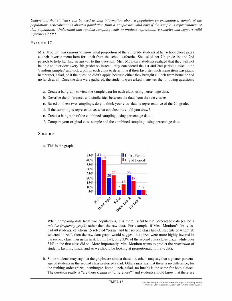
a. This is the graph.

Pizza

Hambu

rger

Salad

Home Lun

ch

No Lunch

5%10%15%20%25%30%35%40%45% 43

20

7

23

7

40

23

1317

7

1st Period2nd Period

When comparing data from two populations, it is more useful to use percentage data (called arelative frequency graph) rather than the raw data. For example, if Mrs. Moulton’s first classhad 40 students, of whom 15 selected “pizza” and her second class had 60 students of whom 20selected “pizza”, then the raw data graph would suggest that pizza were more highly favored inthe second class than in the first. But in fact, only 33% of the second class chose pizza, while over37% in the first class did so. More importantly, Mrs. Moulton wants to predict the proportion ofstudents favoring pizza, and so we should be looking at proportional, not raw, data.

b. Some students may say that the graphs are almost the same, others may say that a greater percent-age of students in the second class preferred salad. Others may say that there is no di↵erence, forthe ranking order (pizza, hamburger, home lunch, salad, no lunch) is the same for both classes.The question really is “are there significant di↵erences?” and students should know that there are


statistical measures of significance, but their use has to be justified in terms of the context. Inthis case, relative to the question posed by Mrs. Moulton, we would conclude that there is nosignificant di↵erence.

c. Of course this is a subjective question, but students should learn that there are statistical measuresof the amount of confidence the researcher can put in these graphs, and again, that use of thosemeasures has to be justified in terms of the context.

d. Accepting the sampling as representative, it is fair to conclude that more than 40% of 7th graderschoose “pizza.”

e. Graph 2 is a relative frequency graph for the combined data, and Graph 3 has put them all together.

f.

Pizza

Hambu

rger

Salad

Home Lun

ch

No Lunch

5%10%15%20%25%30%35%40%45% Combined Results

Pizza

Hambu

rger

Salad

Home Lun

ch

No Lunch

5%10%15%20%25%30%35%40%45% 1st Period

2nd PeriodCombined Results

There is little doubt that, as far as the question (what proportion of 7th grade students prefer pizza?),the conclusion stated in part d is confirmed by either data set and the combined data set. One might gofurther and express confidence in the ordering of the preferences, and that the “significant” disagreementin the “salad” casts doubt on any prediction of the proportion of salad eaters in the class.

What do we mean by a random sample? A random sample is a subset of individuals (a sample) chosen from alarger set (a population). Each individual is chosen randomly and entirely by chance, such that each individual hasthe same probability of being chosen at any stage during the sampling process, and each subset of k individualshas the same probability of being chosen for the sample as any other subset of k individuals. A simple randomsample is an unbiased surveying technique.

In the student workbook homework section 7.2a, students will work on a problem titled Inquiring Students Wantto Know! The premise of the problem is to make a list of topics of student interest and to design a samplingmethod for collecting data from 10 or more randomly selected students. In the teacher notes a recommendation ismade to have students ask every tenth student who comes into the school. This type of sampling is called systemicsampling.

Systematic sampling is an additional statistical method involving the selection of elements from an ordered sam-pling frame. The most common form of systematic sampling is an equal-probability method. In this approach,progression through the list is treated circularly, with a return to the top once the end of the list is passed. Thesampling starts by selecting an element from the list at random and then every kth element in the frame is selected,where k, the sampling interval is calculated as k = N/n, where n is the sample size, and N is the population size.

Using this procedure each element in the population has a known and equal probability of selection. This makessystematic sampling functionally similar to random sampling and is typically applied if the given population islogically homogeneous, because systematic sample units are uniformly distributed over the population.


7MF7-14

Drawing conclusions from data that are subject to random variation is termed statistical inference. Statisticalinference or simply “inference” makes propositions (predictions) about populations, using data drawn from thepopulation of interest via some form of random sampling during a finite period of time. The outcome of statisticalinference is typically the answer to the question “What should be done next?”

Random sampling allows results from a sample to be generalized to the population from which the sample wasselected. The sample proportion is the best estimate, given the constraints of the population proportion. Studentsshould understand that conclusions drawn from random samples can then be generalized to the population fromwhich the sample was appropriately selected. The sample result and the true value from the entire population arelikely to be very close but not exactly the same. Understanding variability in the samplings allows students theopportunity to estimate or even measure the di↵erences.

Use data from a random sample to draw inferences about a population with an unknown characteristic of in-terest. Generate multiple samples (or simulated samples) of the same size to gauge the variation in estimates orpredictions. For example, estimate the mean word length in a book by randomly sampling words from the book;predict the winner of a school election based on randomly sampled survey data. Gauge how far o↵ the estimateor prediction might be. 7.SP.2

The primary focus of 7.SP.2 is for students to collect and use multiple samples of data (either generated or sim-ulated), of the same size, to gauge the variations in estimates or predication, and to make generalizations abouta population. Issues of variation in the samples should be addressed by gauging how far o↵ the estimate orpredication might be.

Was Mrs. Mouton’s technique for gathering data e↵ective? To check on this, and to see how far o↵ the estimatemight be, Mrs. Moulton visits the school district’s food services website and learns the actual percentages of 7thgraders’ consumption over the academic year: 40% favor pizza, 20% favor hamburgers, 10% favor salad, 20%bring a home lunch, and 10% are unaccounted for (which is calculated as having no lunch). This is pretty strongconfirmation. Another approach would be to ask each student in each grade to pick a student at lunch at randomand check what the choice was. This might work, but because of the group of students who bring their own lunchor have no lunch, it could be skewed. In summary, selection of random samples, and representation of the data bygraphs are often questions of taste or common consent.

We often use bar graphs for comparing categorical data and making inferences about populations from the graphs.If comparisons are being made between unequal sized groups, percents give a better basis of comparison. Howeverif the samples are equal in size, then either counts or percents give comparable graphs. For categorical data suchas this, either bar graphs or pie charts are appropriate. If bar graphs are made, they should be called bar graphs,rather than “histograms” because the data are categorical. Histograms are used for graphs that display a range ofnumerical values, such as heights, or ages (which we will discuss further in Section 7.3). Although histograms canbe used in drawing the graph, this may generate graphs that do not truly represent the data, unless each histogramis equal in size.

The variability in the samples can be studied by means of simulation. Although we have used this word before,in a colloquial sense, it is now desirable to work on making the concept somewhat more precise. A simulation isan experiment that models a real-life situation and helps students develop correct intuitions and predict outcomesanalogous to the original problem. Mrs. Moulton wants to create a simulation that models the eating habits of7th graders. Here is her model: she prepares a large non see-through bag, with 200 red skittles (representingpizza), 100 purple skittles (representing hamburgers), 50 green skittles (representing salad), 100 yellow skittles(representing home lunch) and 50 orange skittles (representing no lunch). These proportions are close to theproportions shown in Graph 2. The purpose is to create a population of 500 (representing the amount of studentsin the school) with 40% red skittles for pizza, 20% purple skittles for hamburgers, 10% green skittles for salad,20% yellow skittles for home lunch and 10% orange skittles representing no lunch.

Mrs. Moulton then has students randomly select 10 skittles at a time, repeated roughly five times, returning eachgroup of 10 skittles to the bag each time. Notice that expected values are given. Because approximately 40% ofthe skittles in the bag are red, we should expect to average a draw of 4 skittles. The goal of the activity is thatstudents notice that a random sampling gives close to 40% red skittles.


It is not necessary to replace each skittle individually after it is sampled. In sampling, if less than 10% of thepopulation is sampled at a time, you do not have to sample with replacement. In this case, sampling 10 skittleswill not change the ratio of, i.e., pizza:salad enough to matter. If you are sampling less than 10% of the population,and the sample is random, then independence can be safely assumed. This is called the 10% rule for samplingwithout replacement. Ten skittles are far less than 10% of the skittles in the bag; given the number of skittles ineach bag are 500. Thus, samples of up to 50 without replacement would still be appropriate.

Let’s consider one more scenario. Suppose Mrs. Moulton wishes to investigate the occurrence of pizza demandin her entire school district. A cluster sample could be taken by identifying the di↵erent school boundaries in herschool district as clusters. Cluster sampling is a sampling technique where the entire population is divided intogroups, or clusters, and a random sample of these clusters are selected. All observations in the selected clustersare included in the sample.

A sample of these school boundaries (clusters) would then be chosen at random, so all schools in those schoolboundaries selected would be included in the sample. It can be seen here then that it is easier to call, email, orvisit several schools in the same chosen school boundary, than it is to travel to each school in a random sample toobserve the occurrence of say pizza demand in the entire school district. The big question is: how is the demandfor pizza at Mrs. Moulton’s school similar or di↵erent from that of the school district as a whole?

Scientists use data from samples in order to make conclusions about the world. If using data from the samples, tocome to an agreement on an estimate for the demand for pizza in the school district is calculated by averages, wegive a cautionary note. If the sample sizes are di↵erent, then averaging the data gives more “weight” to the largersamples, so a method will need to be developed to come up with a way to adjust for the di↵erent sample sizes,that is, scaling it up to represent the population of the school district, such as multiplying the estimate by numberof school boundaries in the district.

There potentially could be variability between all the samples taken, i.e. samples taken from a high school versusan elementary school. Variability is a measure of how much samples or data di↵er from each other. How couldwe accommodate for the variability? We would sample only schools that are most similar, i.e. just junior highschools within the chosen school boundary.

Sometimes data are examined to make a table of frequency of the entries. For example, if we want to studythe height of 7th graders, we might collect data (from su�ciently large samples, and make a table showing thepercentage of 7th graders in a given height range (say, counting by inches). In order to get a good estimate, wemight take several samples of the same size. Another use is demonstrated in the course workbook (see section7.2c of Chapter 7) of frequency of letters of the alphabet . Literary sites sometimes use word frequency of text totry to identify the author of the text, based on their knowledge of the word use of a collection of authors. A verynice piece of software allowing for quick visualization of use words is www.tagcrowd.com. A graphic of the 50most common words in the first half of the workbook section 7.3, is displayed on the next page.


7MF7-16

Section 7.3: Draw Informal Comparative Inferences about two Popula-tions

Informally assess the degree of visual overlap of two numerical data distributions with similar variabilities,measuring the di↵erence between the centers by expressing it as a multiple of a measure of variability. Forexample, the mean height of players on the basketball team is 10 cm greater than the mean height of players onthe soccer team, about twice the variability (mean absolute deviation) on either team; on a dot plot, the separationbetween the two distributions of heights is noticeable. 7.SP.3

Use measures of center and measures of variability for numerical data from random samples to draw informalcomparative inferences about two populations. For example, decide whether the words in a chapter of a seventh-grade science book are generally longer than the words in a chapter of a fourth-grade science book. 7.SP.4

The focus of 7.SP.3 and 7.SP.4 is on informal comparative inferences about two populations. In 7.SP.3 we infor-mally assess the degree of visual overlap of two numerical data distributions with similar variabilities, measuringthe di↵erence between the centers by expressing it as a multiple of measure of variability. Practical problemsdealing with measures of center are comparative in nature, as in comparing average scores on the first and secondexams. Such comparisons lead to conjectures about population parameters and constructing arguments based ondata to support the conjectures. If measurements of the population are known, no sampling is necessary and datacomparisons involve the calculated measures of center. Even then, students should consider variability.

Specifically, students will calculate measures of center and spread of data sets, and then use those measures tomake comparisons between populations and conclusions about di↵erences between the populations. The work-books have many problems and activities involving data sets that are easily handled without much computationalsophistication, while adequately exposing the essential ideas to be assimilated.The real power of data analysiscomes out when dealing with large data sets. Here we want to give a flavor of this through two examples, thefirst (Example 18) of which is worked out in detail, and the second is left for class exploration. As the detail inthese examples go beyond the expectations of Standards, we describe the rest of this chapter as an Extension: tobe used for deeper understanding of the material than required by the Standards. In particular, the first examplegoes into the comparison of two data sets through both box plots and the Mean Absolute Deviation, allowing fora comparison of the two methods.

Extension.

Sources of large data sets are readily available online, often with suggestions for classroom computer-basedprojects. Some examples are: the American Fact Finder (Census Bureau; Statistical Universe (LEXIS-NEXIS);Federal Statistics (FedStats); National Center for Health Workforce Analysis (HRSA); CDC Data and StatisticsPage; CIA World Factbook; and locally at Utah Division of Wildlife Resources (UDWR; USGS Water Data forUtah; Utah Statistics (aecf.org) or NSA Utah Data Center; Hawkwatch. In the following, we study in detail a acomparison of two data sets that are large enough to illustrate the power of these methods. This is followed by amore exploratory investigation of data, given in maps.

Research into data sets provides opportunities to connect mathematics to student interests and other academicsubjects, utilizing statistic functions in promethean boards, graphing calculators, or excel spreadsheets; mostespecially for calculations with large data sets. In 6th grade the measures of central tendency (mean, median,mode) were studied, as well as various techniques for summarizing the variability in the data (dot plots, five-number summary and box plots). Here we will introduce a numerical measure of spread: the mean absolutedeviation (MAD). This concept is a little more intuitive and easier to calculate (by hand) than the standard deviationthat will be discussed in grade 10. To illustrate the use of these concepts we will work with a particular data setover the next few pages.


Example 18.

How much taller are the Utah Jazz basketball players than the students in Mr. Spencer’s A3, 7th grademath class?

We will use this context over the next few pages as a vehicle to recall several important statisticalmeasures of spread of data, and further developing their use started in 6th grade. These are: dot plots,histograms, five-number summary, boxplots and the mean absolute deviation (MAD).

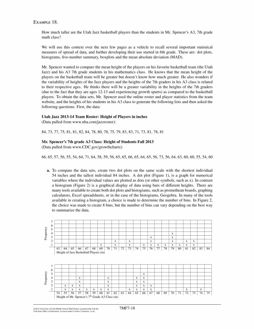
Mr. Spencer wanted to compare the mean height of the players on his favorite basketball team (the UtahJazz) and his A3 7th grade students in his mathematics class. He knows that the mean height of theplayers on the basketball team will be greater but doesn’t know how much greater. He also wonders ifthe variability of heights of the Jazz players and the heights of the 7th graders in his A3 class is relatedto their respective ages. He thinks there will be a greater variability in the heights of the 7th graders(due to the fact that they are ages 12-13 and experiencing growth spurts) as compared to the basketballplayers. To obtain the data sets, Mr. Spencer used the online roster and player statistics from the teamwebsite, and the heights of his students in his A3 class to generate the following lists and then asked thefollowing questions. First, the data:

Utah Jazz 2013-14 Team Roster: Height of Players in inches(Data pulled from www.nba.com/jazzroster):

84, 73, 77, 75, 81, 81, 82, 84, 78, 80, 78, 75, 79, 83, 83, 71, 73, 81, 78, 81

Mr. Spencer’s 7th grade A3 Class: Height of Students Fall 2013(Data pulled from www.CDC.gov/growthcharts):

66, 65, 57, 56, 55, 54, 64, 71, 64, 58, 59, 56, 65, 65, 66, 65, 64, 65, 56, 73, 56, 64, 63, 60, 60, 55, 54, 60

a. To compare the data sets, create two dot plots on the same scale with the shortest individual54 inches and the tallest individual 84 inches. A dot plot (Figure 1), is a graph for numericalvariables where the individual values are plotted as dots (or other symbols, such as x). In contrasta histogram (Figure 2) is a graphical display of data using bars of di↵erent heights. There aremany tools available to create both dot plots and histograms, such as promethean boards, graphingcalculators, Excel spreadsheets, or in the case of the histograms, Geogebra. In many of the toolsavailable in creating a histogram, a choice is made to determine the number of bins. In Figure 2,the choice was made to create 8 bins, but the number of bins can vary depending on the best wayto summarize the data.

Freq

uenc

y

7654 x3 x x2 x x x x x x1 x x x x x x x x x x x

63 64 65 66 67 68 69 70 71 72 73 74 75 76 77 78 79 80 81 82 83 84Height of Jazz Basketball Players (in)

Freq

uenc

y

765 x4 x x x x3 x x x x2 x x x x x x x1 x x x x x x x x x x x x x

54 55 56 57 58 59 60 61 62 63 64 65 66 67 68 69 70 71 72 73 74 75Height of Mr. Spencer’s 7th Grade A3 Class (in)


7MF7-18

54 55 56 57 58 59 60 61 62 63 64 65 66 67 68 69 70 71 72 73 74 75 76 77 78 79 80 81 82 83 84Height of Mr. Spencer’s 7th Grade A3 Class (in) Height of Jazz Basketball Players (in)

Figure 1

Figure 2

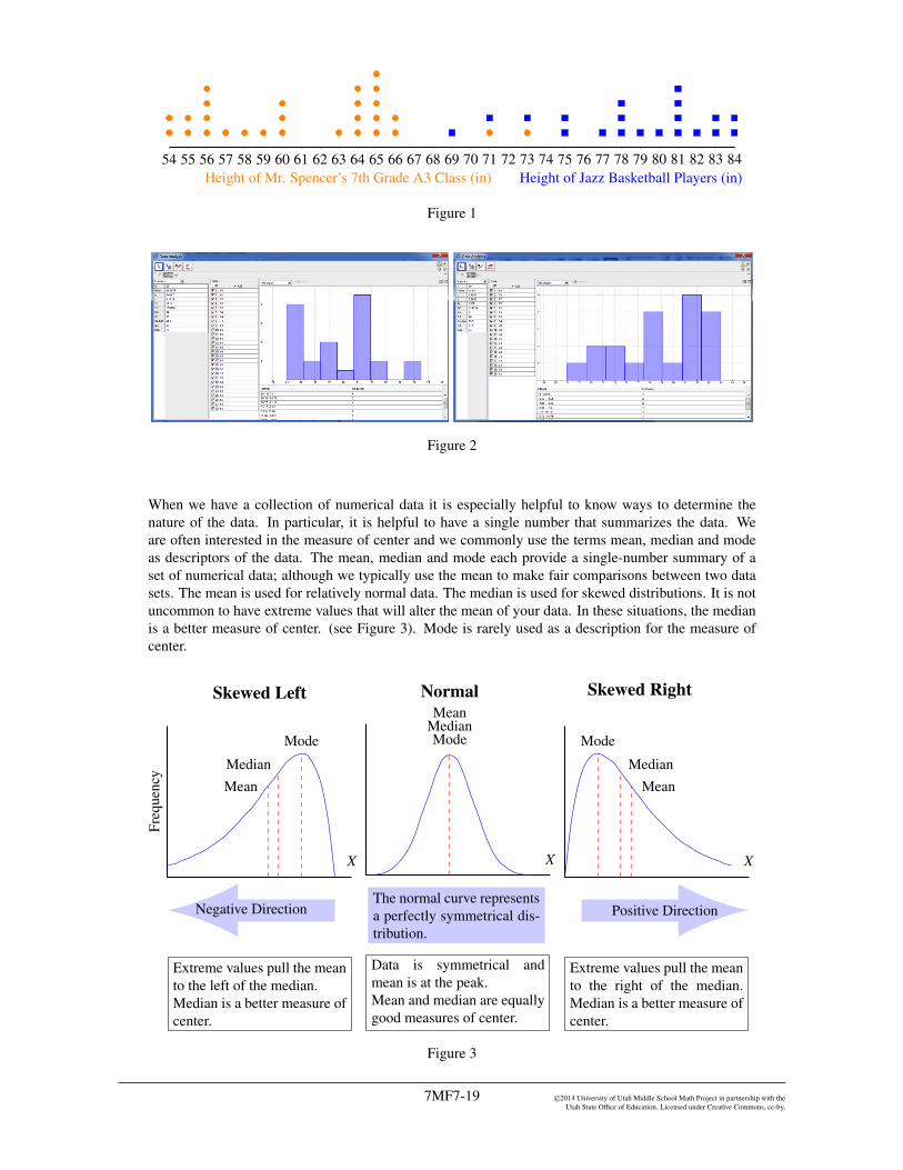
When we have a collection of numerical data it is especially helpful to know ways to determine thenature of the data. In particular, it is helpful to have a single number that summarizes the data. Weare often interested in the measure of center and we commonly use the terms mean, median and modeas descriptors of the data. The mean, median and mode each provide a single-number summary of aset of numerical data; although we typically use the mean to make fair comparisons between two datasets. The mean is used for relatively normal data. The median is used for skewed distributions. It is notuncommon to have extreme values that will alter the mean of your data. In these situations, the medianis a better measure of center. (see Figure 3). Mode is rarely used as a description for the measure ofcenter.

Skewed Left

X

Freq

uenc

y

MeanMedian

Mode

Negative Direction

Extreme values pull the meanto the left of the median.Median is a better measure ofcenter.

Normal

X

ModeMedianMean

The normal curve representsa perfectly symmetrical dis-tribution.

Data is symmetrical andmean is at the peak.Mean and median are equallygood measures of center.

Skewed Right

X

MeanMedian

Mode

Positive Direction

Extreme values pull the meanto the right of the median.Median is a better measure ofcenter.

Figure 3


To calculate the mean, or the average, of a list of numbers, add all the numbers and divide this sum bythe number of values in the list. For example, consider the data set {4, 9, 3, 6, 5}. The mean is

4 + 9 + 3 + 6 + 55

=275= 5.4 .

The mean is an important statistic for a set of numerical data: it gives some sense of the “center ” of thedata set. Two other such statistics, the median and the mode were discussed in 6th grade, but will not beconsidered here. A brief review is found in Section 7.3a homework.

Once we have calculated the mean for a set of data, we want to have some sense of how the data arearranged around the mean: are they bunched up close to the mean, or are they spread out? There areseveral measures of the spread of data; here we concentrate on the mean absolute deviation (MAD).Methods for calculating center and MAD are standards from the Grade 6 curriculum and are beingrevisited in Grade 7 as they compare centers and spreads of di↵erent data sets. The mean absolutedeviation (MAD) is calculated this way: for each data point, calculate its distance from the mean. Nowthe MAD is the mean of this new set of numbers. Let’s do this calculation for the above set of numbers{4, 9, 3, 6, 5}, with mean 5.4.

Data Point Mean Deviation4 5.4 1.49 5.4 3.63 5.4 2.46 5.4 0.65 5.4 0.4

Add the deviations: 1.4+3.6+2.4+0.6+0.4 = 8.4, and divide by the number of data points, 5, to get theMAD = 8.4/5 = 1.68.

Now, let’s apply this technique to the two sets of data Mr. Spencer wants his class to consider. Beforestarting the computation Mr. Spencer asks, based on the representations in Figure 1 above, which of thedata sets seems to have a larger mean absolute deviation (that is, a broader spread).

b. Once the MAD has been calculated, Mr. Spencer asks the class to put the means of the two datasets, and make marks of the place on both sides of the mean that are the MAD away from themean. These insertions tell us directly which data set has the greater spread. The following imageis the result of this work.

54 55 56 57 58 59 60 61 62 63 64 65 66 67 68 69 70 71 72 73 74 75 76 77 78 79 80 81 82 83 84

Mean: 61.29

MAD

�3.16 +3.16

Mr. Spencer’s Class

Mean: 78.85

MAD

�3.16 +3.16

Utah Jazz

This display of the data confirms Mr. Spencer’s hunch: that the data for the Utah Jazz are not spread outas much as the data for his class, and that the spread in his class is symmetric around the mean, while itis more spread in the lower end for the Jazz. What we see in the dot plot that we do not see in the MADdata is the two clusters of heights in Mr. Spencer’s class.

When we use the mean and the MAD to summarize a data set, the mean tells us what is typical or representativefor the data and the MAD tells us how spread out the data are. The MAD tells us how much each score, on average,deviates from the mean, so the greater the MAD, the more spread out the data are.


7MF7-20

A box plot (or box-and-whisker plot) is a visual representation of the five-number summary, and tells us muchmore about the spread of the data, answering questions like: on which side of the mean is there more spread; howfar away the extremes are. Recall these statistics from Grade 6. First, the median is the middle number: there areas many values below the median as there are above. The five number summary shows 1) the location of the lowestdata value, 2) the 25th percentile (first quartile) or the center between the minimum and the median, 3) the 50thpercentile (median), 4) the 75th percentile (third quartile) or the center between the median and the maximum,and 5) the highest data value. A box is drawn from the 25th percentile to the 75th percentile, and ‘whiskers’ aredrawn from the lowest data value to the 25th percentile and from the 75th percentile to the highest data value. Ifthere is no single number in the middle of the list, the median is halfway between the two middle numbers.

As an example we find the five-number summary for the data set: Height of the Utah Jazz BasketballPlayers 2013-14 season.

71 73 73 75 75 77 78 78 78 79 80 81 81 81 81 82 83 83 84 84

Quartile 1 Median Quartile 3

Median is the average of 79 and 80; (79 + 80)/ 2 = 79.5

Quartile 1 (Q1) is the average of 75 and 77; (75 + 77) 2 = 76

Quartile 3 (Q3) is the average of 81 and 82; (81 + 82) 2 = 81.5

The five-number summary is:

Min Q1 Median Q3 Max71 76 79.5 81.5 84

Given the five number summary, we can make the box-plots. Here we show the box plots for both sets ofdata Mr. Spencer wants to compare, and below that the dot plots so that we can compare the informationthat can be obtained from each representation. For example, the box plots show greater spread in Mr.Spencer’s class, and that in both cases the spread of the second quartile is greater than the spread of thethird quartile.

Min=54 Max=73Med=61.5

Q1=56 Q3=65 Min=71 Max=84Med=79.5

Q1=76 Q3=81.5

54 55 56 57 58 59 60 61 62 63 64 65 66 67 68 69 70 71 72 73 74 75 76 77 78 79 80 81 82 83 84Height of Mr. Spencer’s 7th Grade A3 Class (in) Height of Jazz Basketball Players (in)

Example 19.

Glendale Middle School is located in the heart of Salt Lake School District. It is one of five middleschools in the district, and has approximately 835 students recorded in attendance, (data from the 2009-2010 school year). The map shows the boundary of the Salt lake School District, and the arrow pointingto the small blue area is the boundary of the middle school, and the region for the Glendale MiddleSchool is the blue area denoted by the arrow.


Albert R. Lyman Middle School is located in the San Juan School district. In the 2009-2010 school yearthere were approximately 312 students in attendance. The school is located in Blanding, Utah and is theonly middle school in the district. The blue portion highlighted is the San Juan School District.

The State School Board wants to determine how far students travel to school and picked two schools;Albert R. Lyman Middle in San Juan School District and Glendale Middle in Salt Lake City SchoolDistrict. Ten students each, at both schools, were chosen at random and were asked how far theytraveled to school. The responses are below:

Glendale Middle0.10.30.40.60.70.81.21.62.85

Albert R. LymanMiddle0.51.545101218243065

The State School Board asked the students to answer the following questions.


7MF7-22

a. What is the mean of “distance traveled” for each school, and what does the mean represent?

b. What is the mean absolute deviation (MAD) for both schools? Create a table for each data set tohelp with the calculations. Describe what the mean absolute deviation represents?

c. To compare the data sets, create two dots plots on the same scale. What conclusions can bemade from these two data sets? Note: We are only working with data from 10 students andconclusions need to be cautiously represented. Conclusions cannot be made without having anadequate sample size and confirming that the students were chosen at random.


chapter 7 probability and statistics - utah education · pdf filechapter 7 probability and...

Documents