Chapter 7

Duality and Sensitivityin Linear Programming

7.1 Generic Activities versus Resources Perspective

Objective Functions as Costs and Benefits• Optimization models objective functions usually can be

interpreted as minimizing some measure of cost or maximizing some measure of benefit. [7.1]

Choosing a Direction for Inequality Constraints • The most natural expression of a constraint is usually

the one making the right-hand-side constant non-negative. [7.2]

0.3 x1 + 0.4 x2 2.0 (gasoline)

-0.3 x1 - 0.4 x2 -2.0

7.1 Generic Activities versus Resources Perspective

Inequalities as Resource Supplies and Demands • Optimization model constraints of the form usually can

be interpreted as restricting the supply of some commodity or resource. [7.3]

x1 9 (Saudi)

• Optimization model constraints of the form usually can be interpreted as requiring satisfaction of a demand for some commodity or resource. [7.4]

0.4 x1 + 0.2 x2 1.5 (jet fuel)

7.1 Generic Activities versus Resources Perspective

Equality Constraints as Both Supplies and Demands • Optimization model equality constraints usually can be

interpreted as imposing both a supply restriction and a demand requirement on some commodity or resource. [7.5]

Variable-Type Constraints • Non-negativity and other sign restriction constraints are

usually best interpreted as declarations of variable type rather than supply or demand limits on resources. [7.6]

7.1 Generic Activities versus Resources Perspective

Variables as Activities • Decision variables in optimization models can usually

be interpreted as choosing the level of some activity. [7.7]

LHS Coefficients as Activity Inputs and Outputs • Non-zero objective function and constraint coefficients

on LP decision variables display the impacts per unit of the variable’s activity on resources or commodities associated with the objective and constraints. [7.8]

Inputs and Outputs for Activities

Two Crude Example

1000 barrels of Saudi

petroleum processed (x1)

Availability 1000 barrels

Cost $20000

.3 unit gasoline

.4 unit jet fuel

.2 unit lubricants

7.2 Qualitative Sensitivity to Changes in Model Coefficients

Relaxing versus Tightening Constraints• Relaxing the constraints of an optimization model either

leaves the optimal value unchanged or makes it better (higher for a maximize, lower for a minimize). Tightening the constraints either leaves the optimal value unchanged or makes it worse. [7.9]

Relaxing Constraints

1

2

3

4

5

6

1 2 3 4 5 6 7 8

x2

x1

7

8

x1 9

x2 6

1

2

3

4

5

6

1 2 3 4 5 6 7 8

x2

x1

7

8

x1 9

x2 6

Tightening Constraints

1

2

3

4

5

6

1 2 3 4 5 6 7 8

x2

x1

7

8

x1 9

x2 6

1

2

3

4

5

6

1 2 3 4 5 6 7 8

x2

x1

7

8

x1 9

x2 6

Swedish Steel Blending Example

min 16 x1+10 x2 +8 x3+9 x4 +48 x5+60 x6 +53 x7

s.t. x1+ x2 + x3+ x4 + x5+ x6 + x7 = 10000.0080 x1 + 0.0070 x2 + 0.0085 x3 + 0.0040 x4 6.5

0.0080 x1 + 0.0070 x2 + 0.0085 x3 + 0.0040 x4 7.5 0.180 x1 + 0.032 x2 + 1.0 x5 30.00.180 x1 + 0.032 x2 + 1.0 x5 30.5 0.120 x1 + 0.011 x2 + 1.0 x6 10.00.120 x1 + 0.011 x2 + 1.0 x6 12.0 0.001 x2 + 1.0 x7 11.00.001 x2 + 1.0 x7 13.0 x1 75x2 250x1…x7 0

(7.1)

Effect of Changes in RHS

Optimal Value

RHS60.4 75 83.3

9900

9800

9700

9600

9500

9400

x1 75

Current 9526.9

Slope -

Slope -4.98

Slope -3.38Slope 0.00

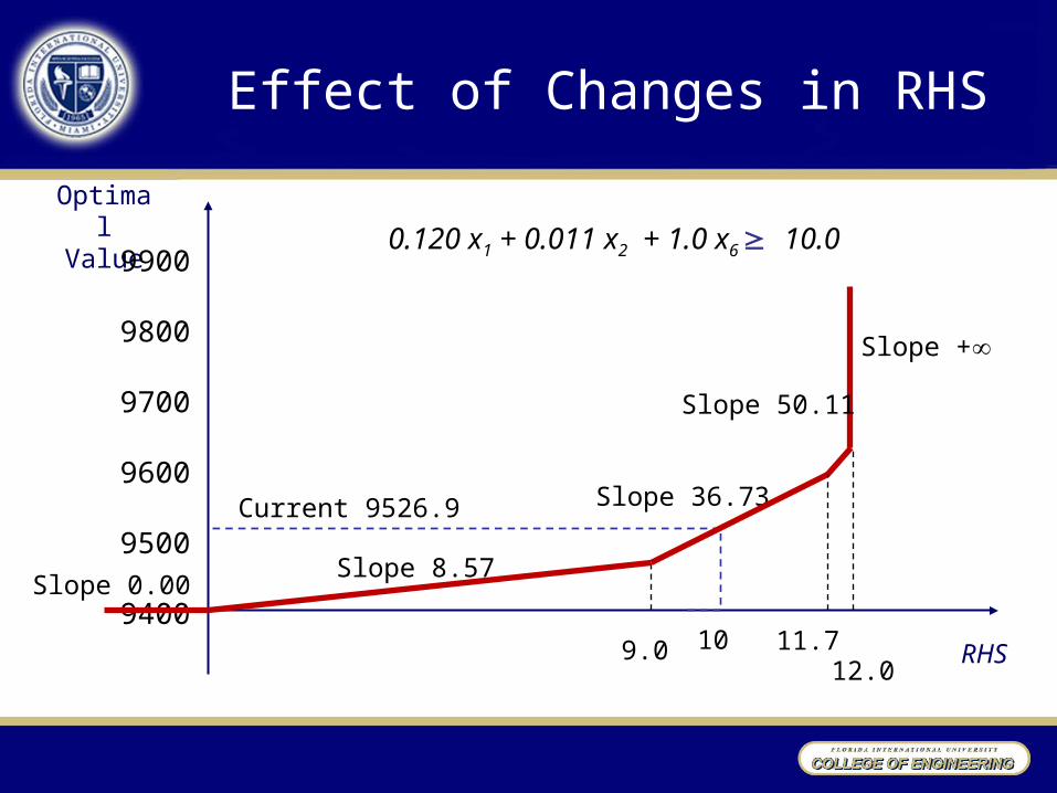
Effect of Changes in RHS

Optimal Value

RHS9.0 10 11.7

9900

9800

9700

9600

9500

9400

0.120 x1 + 0.011 x2 + 1.0 x6 10.0

Current 9526.9

Slope +

Slope 8.57

Slope 36.73

Slope 0.00

Slope 50.11

12.0

Effect of Changes in RHS and LHS

• Changes in LP model RHS coefficients affect the feasible space as follows: [7.10]

• Changes in LP model LHS constraint coefficients on non-negative decision variables affect the feasible space as follows: [7.11]

Constraint Type RHS Increase RHS Decrease

Supply () Relax Tighten

Demand () Tighten Relax

Constraint Type Coefficient Increase

Coefficient Decrease

Supply () Tighten Relax

Demand () Relax Tighten

Effect of Adding or Dropping Constraints

• Adding constraints to an optimization model tightens its feasible set, and dropping constraints relaxes its feasible set. [7.12]

• Explicitly including previous un-modeled constraints in an optimization model must leave the optimal value either unchanged or worsened. [7.13]

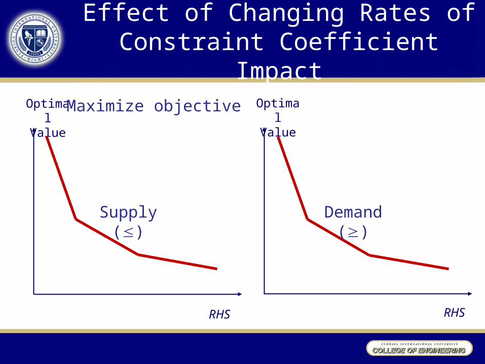
Effect of Changing Rates of Constraint Coefficient Impact

• Coefficient changes that help the optimal value in LP by relaxing constraints help less and less as the change becomes large. Changes that hurt the optimal value by tightening constraints hurt more and more. [7.14]

Effect of Changing Rates of Constraint Coefficient Impact

Optimal Value

RHS

Maximize objective Optimal Value

RHS

Supply()

Demand()

Effect of Changing Rates of Constraint Coefficient Impact

Optimal Value

RHS

Minimize objective Optimal Value

RHS

Supply()

Demand()

Effects of Objective Function Coefficient Changes

• Changing the objective function coefficient of a non-negative variable in an optimization model affects the optimal value as follows: [7.15]

Model Form(Primal)

Coefficient Increase

Coefficient Decrease

Maximize objective Same or better Same or worse

Minimize objective Same or worse Same or better

Changing Rates of Objective Function Coefficient Impact

Maximize objective Optimal Value

coef

• Objective function coefficient changes that help the optimal value in LP help more and more as the change becomes large. Changes that hurt the optimal value less and less. [7.16]

Optimal Value

coef

Minimize objective

Effect of Adding or Dropping Variables

• Adding optimization model activities (variables) must leave the optimal value unchanged or improved. Dropping activities will leave the value unchanged or degraded. [7.17]

7.3 Quantitative Sensitivity to Changes in LP Model Coefficients

Primals and Duals Defined• The primal is the given optimization model, the one

formulating the application of primary interest. [7.18]• The dual is a subsidiary optimization model, defined

over the same input parameters as the primal but characterizing the sensitivity of primal results to changes in inputs. [7.19]

Dual Variables

• There is one dual variable for each main primal constraint. Each reflects the rate of change in primal value per unit increase from the given RHS value of the corresponding constraint. [7.20]

• The LP dual variable on constraint i has type as follows: [7.21]

Primal i is i is i is =Minimize objective i 0 i 0 Unrestricted (URS)

Maximize objective i 0 i 0 Unrestricted (URS)

Two Crude Example

min 20 x1 + 15 x2

s.t.0.3 x1 + 0.4 x2 2.0 : 1 (gasoline)0.4 x1 + 0.2 x2 1.5 : 2 (jet fuel)0.2 x1 + 0.3 x2 0.5 : 3 (lubricants)x1 9 : 4 (Saudi)

x2 6 : 5 (Venezuelan)x1, x2 0

1 0, 2 0, 3 0, 4 0, 5 0

(7.4)

(7.5)

Dual Variables as Implicit Marginal Prices

• Dual variables provide implicit prices for the marginal unit of the resource modeled by each constraint as its RHS limit is encountered. [7.22]

• Variable, 1 , $1000s/1000 barrels, is the implicit price of gasoline at the margin when demand for gasoline is at 2000 barrels.

• Variable, 4 , reflects the marginal impact of the Saudi availability constraint at its current level of 9000 barrels.

Implicit Activity Pricing in Terms of Resources Produced and Consumed

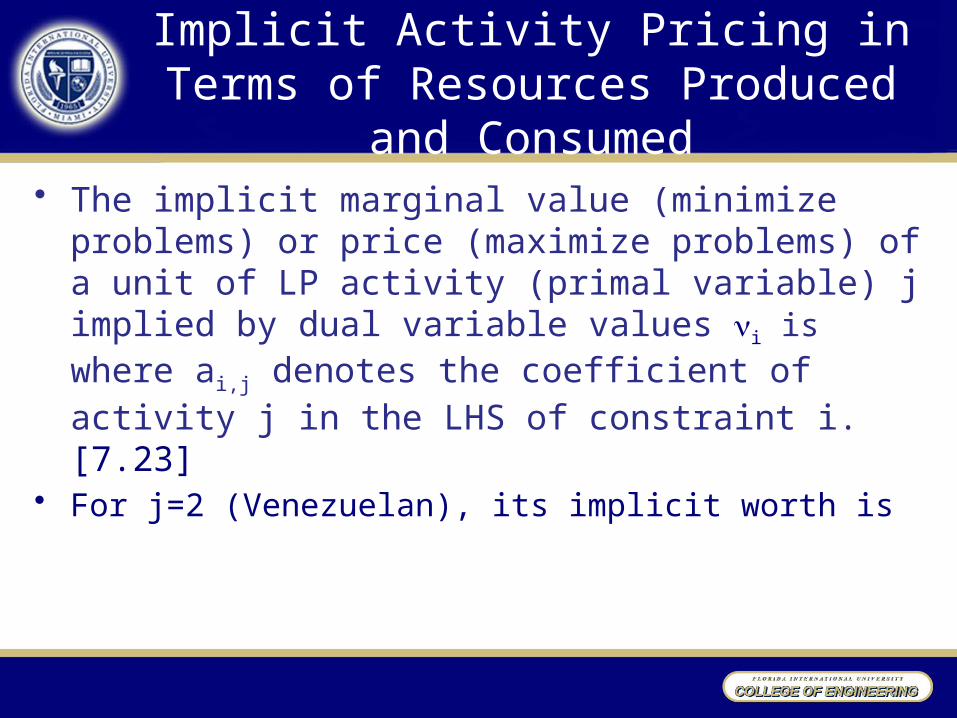
• The implicit marginal value (minimize problems) or price (maximize problems) of a unit of LP activity (primal variable) j implied by dual variable values i is where ai,j denotes the coefficient of activity j in the LHS of constraint i. [7.23]

• For j=2 (Venezuelan), its implicit worth is

Optimal Value Equality between Primal and Dual

• For each non-negative variable activity xj in a minimize LP, there is a corresponding main dual constraint requiring the net marginal value of the activity not to exceed its given cost. In a maximize problem, main dual constraints for xj0 are which keeps the net marginal cost of the activity at least equal to its given benefit. [7.24]

• For the Two Crude model,(7.6)

Main Dual Constraints to Enforce Activity Pricing

• If a primal LP has an optimal solution, its optimal value equals the corresponding optimal dual implicit total value of all constraint resources. [7.25]

• For the Two Crude model,

Primal Complementary Slackness between Primal Constraints and Dual Variable Values

• Either the primal optimal solution makes main inequality constraint i active or the corresponding dual variable =0. [7.26]

• For the primal optimum (2, 3.5) 0.3 (2) + 0.4 (3.5) = 2.0 (active)0.4 (2) + 0.2 (3.5) = 1.5 (active)0.2 (2) + 0.3 (3.5) = 1.45 > 0.5 (inactive)(2) = 2 < 9 (inactive)

(3.5) = 3.5 < 6 (inactive)

3 = 0, 4 = 0, 5 = 0

Dual Complementary Slackness between Dual Constraints and Primal Variable Values

• Either a non-negative primal variable has optimal value xj=0 or the corresponding dual price must make the jth dual constraint (minimize) or (maximize) active. [7.27]

• For the primal optimum (2, 3.5)

are both active.

7.4 Formulating LP DualsForm of the Dual for Non-negative

Primal Variables• The dual of a minimize primal over xj0 is [7.28]

s.t. for all primal activities j

for all primal ’s ifor all primal ’s i

URS for all primal =’s i

7.4 Formulating LP DualsForm of the Dual for Non-negative

Primal Variables• The dual of a maximize primal over xj0 is [7.29]

s.t. for all primal activities j

for all primal ’s ifor all primal ’s i

URS for all primal =’s i

Two Crude Example

Dual:

Max 2+ s.t.

,

(7.7)

Primal:

min 20 x1 + 15 x2

s.t.0.3 x1 + 0.4 x2 2.0 0.4 x1 + 0.2

x2 1.5 0.2 x1 + 0.3 x2 0.5 x1

9 x2 6 x1, x2 0

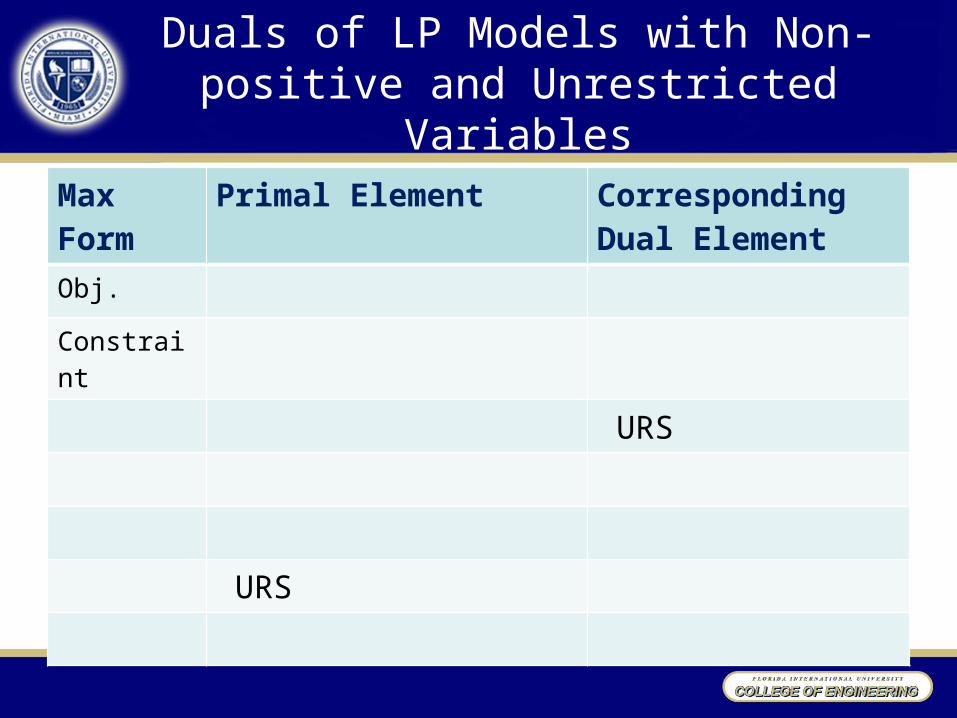
Duals of LP Models with Non-positive and Unrestricted Variables

Max Form

Primal Element Corresponding Dual Element

Obj. Constraint

URS

URS

Duals of LP Models with Non-positive and Unrestricted Variables

Min Form

Primal Element Corresponding Dual Element

Obj. Constraint

URS

URS

Dual of the Dual Is the Primal

• The dual of the dual of any linear program is the LP itself. [7.30]

7.5 Primal-to-Dual RelationshipsWeak Duality between Objective Values

=

Primal objective function – Dual objective function

= (slack in dual constraints)(primal variables) +

(slack in primal constraints)(dual variables)

= (non-positive) + (non-positive) for max OR

(non-negative) + (non-negative) for min

(7.8)

Weak Duality between Objective Values

• The primal objective function evaluated at any feasible solution to a minimize primal is greater than or equal to () the objective function value of the corresponding dual evaluated at any dual feasible solution. For a maximize primal it is (). [7.31]

Strong Duality between Objective Values

• If either a primal LP or its dual has an optimal solution, both do, and their optimal objective function values are equal. [7.32]

Dual Optimum as a By-product

• , – is a pricing vector– is the current basis column matrix of a primal LP– , are the objective function coefficients of the 1st, 2nd,

…, mth basic variables• Optimality has been reached (in min) if

for all variables j• If the revised simplex algorithm stops with a

primal optimal solution, the final pricing vector yields an optimal solution in the corresponding dual. [7.33]

(7.10)

(7.11)

Unbounded and Infeasible Cases

• If either a primal LP model or its dual is unbounded, the other is infeasible. [7.34]

• The following shows which outcome pars are possible for a primal LP and its dual: [7.35]

Primal Dual

Optimal Infeasible Unbounded

Optimal Possible Never Never

Infeasible Never Possible Possible

Unbounded Never Possible Never

7.6 Computer Outputs and What If Changes of Single Parameters

• RHS ranges in LP sensitivity outputs show the interval within which the corresponding dual variable value provides the exact rate of change in optimal value per unit change in RHS (all other data held constant) [7.36]

7.6 Computer Outputs and What If Changes of Single Parameters

• Dropping a constraint can change the optimal solution only if the constraint is active at optimality. [7.39]

• Adding a constraint can change the optimal solution only if that optimum violates the constraint. [7.40]

• An LP variable can be dropped without changing the optimal solution only if its optimal value is zero. [7.41]

• A new LP variable can change the current primal optimal solution only if its dual constraint is violated by the current dual optimum. [7.42]

7.7 Bigger Model Changes, Re-optimization, and Parametric Programing

Ambiguity at Limits of the RHS and Objective Coefficient Ranges• At the limits of the RHS and objective function

sensitivity ranges, rates of optimal value change are ambiguous, with one value applying below the limit and another above. Computer outputs may show either value. [7.43]

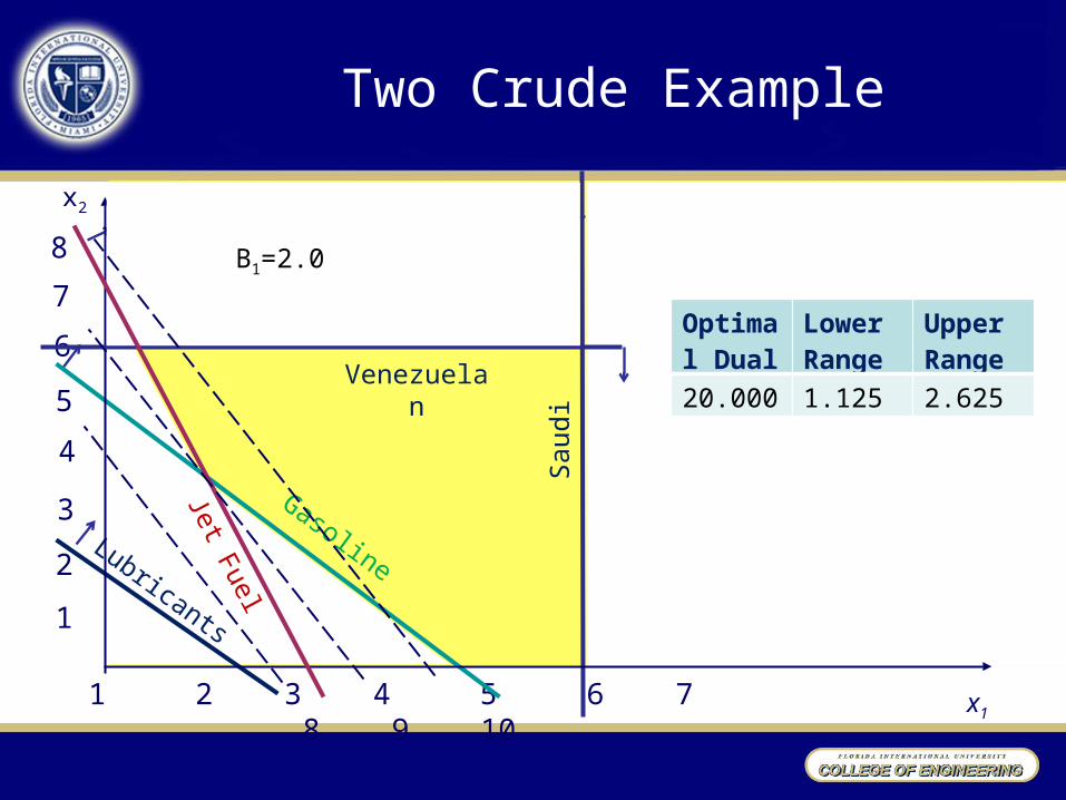
Two Crude Example

1

2

3

4

5

6

1 2 3 4 5 6 7 8 9 10

x2

x1

7

8

Gasoline

Jet Fuel

Lubricants

Sau

di

Venezuelan

B1=2.0

Optimal Dual

Lower Range

Upper Range

20.000 1.125 2.625

Two Crude Example

1

2

3

4

5

6

1 2 3 4 5 6 7 8 9 10

x2

x1

7

8

Gasoline

Jet Fuel

Lubricants

Sau

di

Venezuelan

B1=2.625 Optimal Dual

Lower Range

Upper Range

20.000 1.125 2.625

Optimal Dual

Lower Range

Upper Range

66.667 2.625 5.100

Two Crude Example

1

2

3

4

5

6

1 2 3 4 5 6 7 8 9 10

x2

x1

7

8

GasolineJet Fuel

Lubricants

Sau

di

Venezuelan

B1=3.25

Optimal Dual

Lower Range

Upper Range

66.667 2.625 5.100

Connection between Rate Changes and Degeneracy

• Rates of variation in optimal value with model constants change when the collection of active primal or dual constraints changes. [7.44]

• Degeneracy, which is extremely common in large-scale LP models, limits the usefulness of sensitivity by-products from primal optimization because it leads to narrow RHS and objective coefficient ranges and ambiguity at the range limits. [7.45]

Re-Optimization to Make Sensitivity Exact

• If the number of “what-if” variations does not grow too big, re-optimization using different values of model input parameters often provides the most practical avenue to good sensitivity analysis. [7.46]

Parametric Variation of One Coefficient

• Parametric studies track the optimal value as a function of model inputs.

• If the number of “what-if” variations does not grow too big, re-optimization using different values of model input parameters often provides the most practical avenue to good sensitivity analysis. [7.46]

Parametric Variation of One Coefficient

• Parametric studies track the optimal value as a function of model inputs.

• Parametric studies of optimal value as a function of a single-model RHS or objective function coefficient can be constructed by repeated optimization using new coefficient values just outside the previous applicable sensitivity range. [7.47]

Parametric Variation of One Coefficient:Two Crude Example

Optimal Value

RHS1.1 2.62.0

250

150

50

Slope +(infeasible)

Slope 20.00

Slope 0.00

Slope 66.67

5.1

92.5

Case RHS Dual Lower Rang

Upper Range

Base Model

2.000 20.000 1.125 2.625

Variant 1 2.625+ 66.667 2.626 5.100

Variant 2 5.100+ + 5.100 +

Variant 3 1.125- 0.000 - 1.125

Assessing Effects of Multiple Parameter Changes

• Elementary LP sensitivity rates of change and ranges hold only for a single coefficient change, with all other data held constant. [7.48]

• If demand increase in jet fuel (b2) is twice as the increase for gasoline (b1).

b1new = (1+) b1

base

b2new = (1+2) b2

base

binew = bi

base + bi

b1=2.0

b2=3.0

(7.14)

Assessing Effects of Multiple Parameter Changes

The effect of a multiple change in RHS with step can be analyzed parametrically by treating as a new decision variable with constraint coefficient -bi that detail the rates of change in RHS’s bi and a value fixed by a new equality constrain. [7.49]

min 20 x1 + 15 x2

s.t. 0.3 x1 + 0.4 x2 - 2 2.0 0.4 x1 + 0.2 x2 - 3 1.5 0.2 x1 + 0.3 x2 0.5 x1 9

x2 6 = b6

x1, x2 0, URS

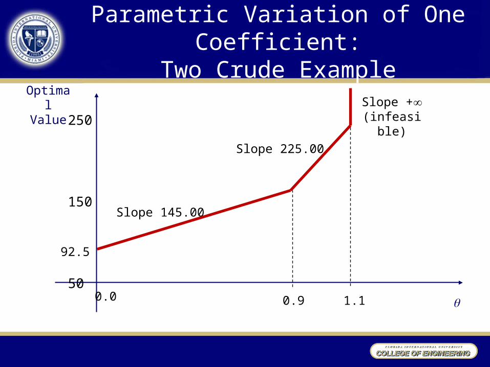
Parametric Variation of One Coefficient:Two Crude Example

Optimal Value

0.90.0

250

150

50

Slope +(infeasible)

Slope 145.00

Slope 225.00

1.1

92.5

Parametric Change of Multiple Objective Function Coefficients

• The effect of multiple change in objective function with step can be analyzed parametrically by treating objective rates of change -ci as coefficients in a new equality constraint having RHS zero and a new unrestricted variable with objective coefficient . [7.50]