chapter 6 - uc santa barbara geography · chapter 6 the previous chapter presented descriptive...

Chapter 6

The previous chapter presented descriptive statistics of the household sample and

explored potential relations between farm and household characteristics and forest

clearing and land use among small farmers in the SLNP. This chapter will investigate the

separate effects of these factors on the outcomes of land use and deforestation by colonist

farmers through statistical modeling, specifically, multiple regression (MR) analysis.

Composite time-series Landsat TM satellite images (Chapter 1), descriptive

community (Chapter 4) and household data (Chapter 5) agree that, as elsewhere in the

tropics, small farmer agricultural expansion is the proximate cause of forest clearing in

the SLNP. Colonist farmers convert forest to a host of agricultural land uses, each with a

potentially distinct impact on forest conversion. Unlike frontier environments in other

tropical lowland environments in Latin America (particularly in the Amazon basin, but

also, to a lesser extent, in neighboring Belize and Mexico), in the SLNP colonist farmer

land use is relatively homogeneous. Virtually all the farmers grow maize and little else,

and a third of them have a few head of cattle. Thus, the descriptive data from Chapters

Four and Five indicate that the vast majority of forests cleared in the SLNP have been

converted directly to maize fields which ultimately become fallow land.

Variations across households in land use are much smaller in this sample

compared to many similar studies in other frontier regions in Latin America. With a

remarkably uniform land use of maize and few significant additional land uses as found

in other frontier regions, in the form of market crops and perennials with widely diverse

land demands (save cattle among a quarter of the sample), complex relations between

humans and the land are greatly reduced in the SLNP. Therefore, household variability

194

in land cleared may be more strongly predicted by demographic, political-economic,

socio-economic, and ecological factors, and usefully modeled in a direct relation.

Since forest conversion is a function of farmer land use, modeling forest clearing

only does not take into account the various land uses for which a farmer has cleared his

land. Therefore, in addition to presenting a model on forest clearing and on the percent

of forest cleared on a farm holding, I will present MR models with the four major land

uses for farms in the sample: maize, fallow, forest, and pasture. As only a quarter of the

farms in the sample have cattle, the latter model will be a logistic regression (LR), which

will produce likelihood ratios of membership in the “pasture” group. This is an important

model since households with pasture have cleared, on average, twice as much land as

those without pasture (see Figure 6.1). Amount of land in pasture and whether or not a

farm has pasture are highly significant variables in the cleared land and percent of farm

cleared models but are excluded due to concerns of endogeneity.

The first section of this chapter describes the selection of predictor variables

based on theoretical considerations and on their impact on the predictive power of the

models. The following section explains hypotheses regarding the relations between the

predictors selected and land use outcomes. Model specifications for the six final models

are discussed next, including some of the diagnostics used to assess potential violations

of model assumptions. Lastly, the six models will be presented and their results

interpreted.

A. Selection of Variables

The models in this chapter were designed to capture patterns of farmer land use

and land clearing in the SLNP region while also considering these relations to theory.

The variables examined were selected from the literature presented in Chapter Two, from

surveys in the Ecuadorian Amazon (e.g., Bilsborrow and Pan, 2001) and the Mexican

Yucatán (e.g., Klepeis and Turner II, 2001), and were designed to fit the study area with

help from Norman Schwartz, Pro-Petén-Conservation International (Corzo-Márquez and

Obando, 2000), Jorge Grunberg of CARE (Macz and Grunberg, 1999), Edgar Calderón

Rudy Herrera and Edgar Calderón of The Nature Conservancy (The Nature Conservancy,

1997), and by members of the Guatemalan agro-forestry aid institute, Centro Maya.

195

Lastly, variables were derived from additions and modifications of earlier instruments

with the help of my Peténero interview team and from many long discussions with

community leaders in the SLNP. Based on the literature on tropical frontier deforestation

and knowledge of local conditions, the overarching hypothesis was that deforestation for

agricultural extensification is related to a host of conditions thought to be important in

frontier environments. Generally these conditions included factors such as family size

and composition, and availability of land, and of human, social, and labor capital.

The first step taken in the data analysis for this chapter was to analyze sets of

predictors by category using sequential multiple regression. Several hundred variables

from head of household surveys were initially considered for inclusion in the models.

Following considerations of theory and data quality, this number was reduced to 104

variables that were probed with descriptive analyses such as means, medians,

frequencies, and standard deviations. From this second set, approximately seventy-five

variables were selected for descriptive analysis in Chapter Five via cross-tabulations.

It was from this last iteration in the winnowing process that I ran many sequential

regressions to trim the models to their current form, again based on theoretical concerns

and model fit. In examining potential contributions of predictors to the models, several

measures were used, including R2 values, t-ratios, and the sign of the Beta coefficients as

related to prior expectations. First, as I am particularly interested in demographic effects,

given the proposed connection in this dissertation between migration and land use, twelve

demographic variables were tested against each other in each of the models. Consistently

insignificant independent variables were usually removed, unless theoretical importance

compelled me to retain them. Following the analysis of relations among demographic

variables, and between them and each of the six outcome variables, variables from other

categories were included in the model. Sixty household and farm characteristic variables,

five political-economic variables, and three ecological variables were each included

sequentially in the model, one set after another. I then combined all variables that were

significant at the 0.15 level in most of the models at the set level together in six large

“full” models. I further paired down the full models by omitting variables that were

insignificant at the 0.15 level in the majority of the models. Again, variables remained in

196

several cases because of theoretical considerations even though they were insignificant

predictors of the outcome variables.

Once I had six completed models, a pattern emerged that merited further

attention. The models for Pasture and Cropland were behaving differently from the

other four models. I therefore redid the process described above for each of these two

models. I changed the independent variables to produce a better fit for the logistic model

Pasture. I justify doing so for three reasons. First, the Pasture model probes a

fundamentally different question (a question of membership) than the other land use

models (questions of extent). Second, cattle ownership is qualitatively a different kind

of land use than is maize farming. And third, only a quarter of the sample own cattle,

suggesting a selective or different group of farmers. The resulting model produced a

noticeably higher R2 value than when the same set of predictors from the other five

models was employed. However, because virtually all farmers have land in crops, and it

is a major component of overall cleared land, I ultimately decided to keep the same

independent variables for this model as for the other multivariate regression models with

one exception.

B. Definitions of Variables and Hypotheses

The hypothesized relations between the predictor variables and land use by settler

households are summarized in (Table 6.1.). These hypotheses come from the literature

on colonization and deforestation in the Latin American tropics in general (Chapter 2),

and in Petén, Guatemala specifically (Chapter 1). A plus or minus sign is assigned to

indicate the anticipated direction of the relation between the predictors and land use

outcomes. Each suite of factors is described in this section. Where predictor variables

were excluded in the pasture model, they are shaded in gray in Table 6.1.

The land use outcomes feature three mutually exclusive variables: cropland,

fallow land, and forest; an aggregate land use variable, cleared land; a composite

variable, percentage of land cleared; and a dichotomous variable, cattle ownership. The

vast majority of farms in the sample are comprised entirely or almost entirely of cropland

(virtually all in maize), fallow, and forest. Though farmers in the region use manzanas

197

(0.7 hectares), all measurements are converted to the metric units of hectares for

comparison to other regions.

Since the aggregate variable, Cleared land, is a direct measure of a household’s

impact on the forest, summing up all of its land uses, it is included as an outcome

variable. The percentage of land cleared is included as a dependent variable as well.

The latter is a key variable to examine since it contains farm size in the denominator.

This is useful as it is expected that more land leads to more of each land use. But the

percent of each land use indicates trade-offs in the decision-making process. I will now

discuss hypotheses related to the independent variables that were ultimately selected for

the six models of land use and land cover in the SLNP.

1. Demographics Factors

Household size is expected to be positively related to agricultural extensification

principally for two reasons. First, more mouths to feed stimulates greater demand for

production. Second, more hands to work the farm means that production may be

increased through extensification without hiring labor outside the household. These

arguments hark back to Malthus (1873) and Chayanov (1986). More recently they were

corroborated in Latin American frontier environments (Pichón, F.J., 1997; Rosero-Bixby

and Palloni, 1998). Yet it may be expected that household size is negatively related to

the most extensive land use, pasture, since livestock activities should depend more on

farm size than on number of farm laborers (as discussed by authors featured in Chapter

Two, e.g., Mac Donald, 1981; Hecht, 1983; De Walt, 1985; Buschbacher, 1986; Shane,

1986; Joly, 1989; Loker, 1993; Hemming, 1994; Fujisaka et al., 1996; Humphries, 1998;

Walker et al., 2000).

2. Political-economic Factors

Contact with an NGO is dichotomous (0 = no contact, 1 = some contact). This

variable measures whether or not a farmer has had any contact with a conservation or

development organization (whether NGO or GO). I am uncertain as to the potential

relation between contact with an NGO and land use. To the extent that such contact is

with an environmental NGO or government agricultural organization promoting

198

conservation and sustainable agriculture, it is expected to be associated with less forest

clearing, less land in fallow, crops, and pasture, and more land in forest (as found in

Brazil by Almeida, 1992). However, contact with agricultural extension agents and

credit lending agencies could be related to a farmer purchasing cattle or adopting

technologies that make land use more profitable, possibly leading to more clearing.

No land title is defined as the absence of any credible claim to legal ownership of

the farm. This includes not completing any of the steps necessary for acquiring a legal

title, such as having solicited a request for land ownership to INTA (The National

Institute for Agrarian Reform), having the farm measured by INTA (or a professional

surveyer), or having a provisional title. Only farms outside the core zone of the park or

farms that are part of cooperatives (the two together represent 31% of the sample) are

able to assert legal claims to their farms on an individual or collective basis.

Following the debate by several authors mentioned in Chapter Two (e.g.,

Thiesenhusen, 1991; Fearnside, 1993; Kaimowitz, 1995; Clark, 1996), I anticipate that

having legal claim to the farm is associated with less forest clearing. Particularly, it is

anticipated that relatively less land will be sown in crops. With a legal claim, a farmer

may invest in crop intensification while for squatters agricultural intensification makes

little sense if a farmer anticipates he may abandon the farm or be evicted from it in the

near future. However, land titling also enables a farmer to avail himself of credit which,

given farmer desires, is likely to be invested in purchasing cattle. Thus, were it not for

the influence land title may have on cattle adoption, I would anticipate the total amount

cleared and the percentage cleared to be positively associated with lack of secure land

title. In sum, I expect lack of secure land title to be associated with extensification in the

form of cropland and fallow land while the relation to cleared land and percent cleared

could be positive or negative.

3. Socio-economic Factors

Household socio-economic characteristics

Ethnicity is a dichotomous variable measuring membership or not in an

indigenous group (one quarter of the sample is indigenous, divided more or less evenly

between Q’eqchí Maya and other Maya groups). It is an open question as to how

199

ethnicity might affect land use on the frontier. I suspect it will be insignificantly related

to most outcomes. As mentioned in Chapter Five, cross-tabular analyses indicated only a

modest relation between ethnicity and agricultural extensification. However, this topic

deserves further consideration given that most of Petén’s population, especially its small

farmers, is Maya. I therefore include the variable in the models. The findings will add to

the small literature that has examined the influence on forest clearing of indigenous

versus non-indigenous colonists (Atran, 1999; Corzo-Márquez and Obando, 2000; Fagan,

2000; Carr, forthcoming-a).

Educational achievement is dichotomous: it indicates whether or not the

household head has ever attended school. Since nearly half the heads of household have

never attended school, this measure was chosen over a continuous variable representing

years or levels of schooling attained. It is uncertain if educational achievement is related

to extensification, intensification, or both. The educational achievement of the head of

household could have a positive effect on agricultural extensification if education leads to

a higher motivation to increase living standards through increasing production. However,

production could be increased by intensification if education increases means an

increased knowledge of farm management techniques such as the ability to read

instructions on fertilizer and herbicide applications (e.g., Moran, 1984; Godoy et al.,

1998). An alternative is that education is related to a greater level of environmental

awareness, and may be expected to reduce agricultural extensification. However, few

SLNP farmers thought that the park’s conservation should inhibit their farming (Chapter

5).

In the Ecuadorian Amazon, Pichón (1997) found that educational achievement of

the household head was weakly negatively associated with percent of land in forest and

positively related to land in pasture. This was interpreted as more education being

associated with the ambition to own cattle. Given that the “culture of pasture” described

in Chapter Two appears to exist among SLNP colonists, probably a good measure for

farmer’s ambitions in general is whether or not they desire to have cattle or not).

Land in previous residence is a continuous variable expressing the amount of land

available to the household in its previous residence (most respondents had no land). This

category includes legally owned land or land on which the household had homesteader’s

200

rights. Only 2% of the sample had legal title to their land and almost 70% had no land to

farm in origin areas.

Having access to land in previous residence suggests greater farming knowledge,

which may be associated with more forest clearing for market production. Further, given

the extreme poverty of the sample and the likely inability of farmers to purchase land in

settled communities, access to land prior to migrating may imply having lived in former

land abundant frontier regions where swidden farming was learned. It is therefore

expected to exert a positive effect on extensification.

Lastly, for those with access to land in origin areas, the household came not to

obtain land, as did most, but to expand landholdings. In this way, migration to the SLNP

may be viewed as a form of agricultural extensification. Presumably, those who enjoyed

land ownership prior to settlement in the SLNP area relinquished their land rights with

the intention to farm more land in the SLNP and to invest in livestock or crops primarily

for market sale.

A household head is considered to have engaged in Off-farm labor if he worked

off the farm for a wage any time during the previous 12 months. As described in Chapter

Five, this usually means working on nearby farms on a day by day basis as a hired field

hand. Presumably, if the household head engages in work off the farm, less time can be

devoted to working on one’s own farm. Therefore, off-farm labor is expected to have a

negative relation with agricultural extensification (this relation was found in the

Ecuadorian Amazon: Pichón, F.J., 1997; Bilsborrow and Pan, 2001).

The variable, Rents land, is dichotomous and refers to households that work a plot

in exchange for money, crops, labor, or for free (as is often the case with a landless friend

or relative). Households that rent land are expected to dedicate a much greater proportion

of their farm-holdings to crop production (e.g., Shriar, 1999). Renters typically have

small plots, often little more than a few manzanas for subsistence production. Because of

these small plots, little absolute forest clearing is expected among renters, but a much

greater proportion of land cleared and in crops is hypothesized. Because fallow land

would take away from precious land that could be dedicated to crops, in the case of very

small rented plots, it is expected that farmers will leave very little land in fallow. Further,

in some cases, as mentioned in Chapter 4, renters farm a plot for only a year or two, often

201

in exchange for clearing the forest for larger landholders who intend to sow pasture grass.

Usually, renters will have no fallow land since they will rent only enough land for actual

crop use.

Farm characteristics

Size of total holdings is expected to be a powerful predictor of land use. Simply,

the larger the farm, the more land that is cleared; but the larger the farm, the more land

may also be conserved and maintained in forest. Large farms are therefore expected to

have more land in all major land uses, i.e., forest, crops, and fallow, but a lower

percentage of their farm cleared for crops and fallow. Labor limitations constrain the

percentage of land that can be cleared more than does farm size once the farm is over a

certain size, perhaps twenty hectares. Larger farms are also anticipated to be associated

with cattle ownership since cattle are highly land-demanding (e.g., Mac Donald, 1981;

Hecht, 1983; De Walt, 1985; Buschbacher, 1986; Shane, 1986; Joly, 1989; Loker, 1993;

Hemming, 1994; Fujisaka et al., 1996; Humphries, 1998; Walker et al., 2000).

Conversely, small farms are expected to be associated with less land in each of

the land uses and to be associated with little cattle ownership and a greater percentage of

the farm cleared, particularly in crops (and a smaller percentage in forest and fallow). As

noted in Chapter Five, the latter is expected because subsistence requires a minimum

amount of land to be cropped regardless of size of total holdings.

Distance to road is measured in kilometers by footpath from each farmer’s

principal farm-holding to whichever is closest between the Naranjo and Bethel roads, the

only two roads offering access to the core zone of the park. Several studies in the Latin

American tropics have noted the inverse relation between deforestation and distance to

road at the regional level (e.g., Rudel and Horowitz, 1993; Fujisaka et al., 1996; Nelson

and Hellerstein, 1997; Pichón, F.J., 1997; Sader et al., 1997).

I expect farm distance to a road to be negatively associated with total and

percentages of forest cleared and land in crops and fallow when farm size is included in

the model. I expect distance to road to be negatively related to cattle ownership for two

reasons. Pasture is associated with legal claim to the farm which is more likely among

earlier colonists located closer to a road. Secondly, distance to a road should be

202

negatively associated with the value of the farm since transportation costs make

successful farming more difficult. Therefore farmers who are able to afford cattle are

more likely to have farms located in desirable locations closer to the road.

Further, as discussed in Chapters Two and Five, distance to the road is negatively

related to duration on the farm, and thus cleared land, particularly land in fallow (newer

farms have yet to complete their crop:fallow cycle). When duration is controlled for in

the models, again, I anticipate road proximity to be a proxy for market access, and to

therefore be positively related to all categories of cleared land. Nevertheless, a

reasonable alternative hypothesis is that the cost of transporting agricultural products to a

road may encourage more crops to be grown in compensation.

Duration on the farm is a categorical variable equal to “0”, households occupying

their farm for fewer years than the mean, and “1”, households occupying their farm for

longer than the mean number of years. A continuous variable for duration on the farm

was insignificant in the full models in which other variables apparently diminished its

significance (e.g., household size, farm size, and distance to road). This is likely at least

partially due to the low variability across the sample in farm duration. It appears that

duration may not have a strong affect in itself until a certain number of years on the farm

has been reached since it takes several years for crops to be planted and at least one

fallow rotation to be completed.

Duration on the farm is expected to be related to agricultural extensification and

cattle ownership. Evidence of land consolidation in the evolution of frontiers

corroborates this expectation (Almeida, 1992). Similar to trends reported by Murphy and

others (1997) in Ecuador and Almeida (1992) in Brazil, it appears from data presented in

Chapter Four and Five that earlier arrivals to the SLNP selected the best locations for

farms in terms of natural endowments such as flat land, and the availability of water, and

in terms of proximity to roads. These households may be more likely to take advantage

of their farm’s geography by expanding production through forest clearing. More

importantly, longer duration on the farm allows for more years of land clearing and the

desire for owning more cattle to be realized.

Additional agricultural fields is defined as any household with more than one

farm plot. Additional agricultural fields are expected to be associated with greater forest

203

clearing and with cattle ownership. I expect that the use of an additional field implies a

desire to expand crop production or to have cattle on one plot and crops on another.

Simply, if a farmer seeks to add a plot to his overall landholdings, most likely he is doing

so to use it for a productive purpose. Indeed, in the informal land “market” of the SLNP,

not using the land would invite squatters to claim it as theirs.

The cropping of the nitrogen-fixing legume, velvet bean, and the application of

herbicides are the two most common types of intensification in the region. Only 11% of

the sample use any other form of intensification, such as chemical fertilizers. Velvet

Bean and/or herbicides is a categorical variable with 0 assigned to households who use

neither intensification technique, 1 for households which employ one or the other, and 2

to households employing both.

As addressed in Chapter Two, intensification should allow greater production in

less area. Indeed, it may encourage a reduction in cropland due to increased labor

investment per unit space (e.g., Geertz, 1968; Turner II et al., 1977; Lundahl, 1981;

Bilsborrow, 1987; Brush and Turner II, 1987; Martine, 1990; Collier and Horsnell, 1995).

Thus, given that there is little leisure time among SLNP farmers (Chapter 4), labor

invested in intensification may compete directly with labor invested in extensification,

reducing pressure on farm forests.

The use of velvet bean allows the compression of fallow rotations, and the

application of herbicides facilitates cropping in successive years (see, e.g., Mausolff and

Ferber, 1995; Shriar, 1999). Therefore, these forms of intensification are expected to be

negatively related to land in fallow. However, it is possible that agricultural

intensification may ultimately promote extensification since producing more on less land

can free up land for cattle expansion (Zweifler, 1994).

Assets is a categorical variable defined as ownership of a radio, a horse, a car, or a

chainsaw. One point is assigned to each asset. Assets are expected to be positively

associated with forest clearing for crops and pasture (e.g., Almeida, 1992; Rudel and

Horowitz, 1993; Murphy et al., 1997; Mather et al., 1999). More assets reflect the ability

of a farmer to hire laborers to clear land and harvest crops, and to purchase cattle. It may

also reflect on previous ambitious, market-oriented behavior.

204

4. Ecological Factors

Soil fertility is a dichotomous variable: 0 for those without fertile soil and 1 for

those with fertile soil. This measures the perception of farmers relative to the overall

quality of soil conditions on their farm and therefore conflates potential variability in soil

quality within farms and is not corroborated by physical measurement. Soil fertility is

expected to be positively associated with forest and cropland and negatively related to

cleared land, percentage of land cleared, land in fallow, and cattle ownership.

As discussed in Chapter Two, an overwhelming number of cases of rapid

deforestation reported in the Latin American tropics have involved pasture expansion

following soil degradation (Hecht, 1985; Moran et al., 1994; Pichón, F.J., 1997). Pasture

expansion often makes forest conversion irreversible and tends to spur further forest

clearing as soils are rapidly weathered (Mac Donald, 1981; Hecht, 1983; De Walt, 1985;

Shane, 1986; Eden et al., 1990; Loker, 1993; Walker et al., 2000).

Conversely, farmers with better soils may be encouraged to favor cropland over

pasture (and, therefore, over forest) since pasture grass will survive on impoverished soils

for years after the soil is too exhausted for successful crop production (e.g., Hecht, 1983).

Lastly, as in most farming regions, farmers appear to prefer flat land when

choosing where to clear land. Presumably then, farms with Flat land were selected

preferentially for agricultural expansion farms than farms of greater relief. It would then

follow that these farms would have more forest cleared and more land in crops and

fallow.

C. Model Design

The first six models are standard multiple regressions (MR). Multiple regression

is an extension of bivariate regression. The main difference is that multiple independent

variables (instead of one) are combined to predict the value of the dependent variable (for

more on multivariate methods, see, e.g., Tabachnick and Fidell, 1996). The results of

MR yield an equation that represents the best prediction for a dependent variable from a

set of continuous or dichotomous independent variables. The equation takes the general

form:

205

kk XBXBXBAY ...2211 +++=

where Y is the vector of dependent variables (DVs), A is the intercept, the Xs are the

independent variables (IVs), and the Bs are the coefficients assigned to each predictor

during the regression. The purpose of regression analysis is to demonstrate relations

among variables, but such relations do not indicate causality. Theoretical and empirical

knowledge external to the regression analyses is necessary for credible speculations as to

potential causal relations among variables in the model.

For the specific DVs analyzed here, the equation takes the form:

where each Y is the value of dependent variables for land in maize, fallow, forest, cleared

land, and percent of land cleared at the farm level, A is the intercept for each dependent

variable, the Xs are the independent variables for each DV and the Bs are the coefficients

assigned to each IV.

Each independent variable was evaluated relative to its contribution to the model

after all the other IVs are entered. Thus, each independent variable is assessed by what it

adds to the prediction of the DV, that is, different from, or “over and above,” the

predictability provided by all other IVs. It is therefore possible for a variable to appear

unimportant in the model when it is actually highly correlated with the dependent

variable.

Green (1991) offers an in-depth treatment of required sample size. For testing

multiple correlation, the simple rule of thumb for minimum sample size relative to the

number of independent variables in the model is that n (sample size) should be equal to or

greater than 50 + 8*m (where m = the number of IVs). For testing the relation of

individual predictors to the dependent variable in the model, n should be equal to or

greater than 104 + m. The sample size here of 241 exceeds 170 in the first case. In the

second case 241 exceeds 119. These rules assume a “medium size” relation between the

IVs and DV of alpha equal to 0.05 and Beta equal to .20, a rule that is met with all but a

,...1111__ kkoutcomeuseland XBXBXBA +++=y

206

handful of IV-DV relations. Still, even employing the more conservative estimate for

minimum sample size, requiring 15 cases per predictor, 241 still exceeds 225, or 15

multiplied by the maximum number of IVs (15) in the models.

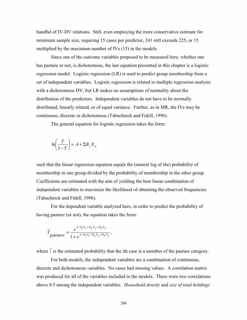
Since one of the outcome variables proposed to be measured here, whether one

has pasture or not, is dichotomous, the last equation presented in this chapter is a logistic

regression model. Logistic regression (LR) is used to predict group membership from a

set of independent variables. Logistic regression is related to multiple regression analysis

with a dichotomous DV, but LR makes no assumptions of normality about the

distribution of the predictors. Independent variables do not have to be normally

distributed, linearly related, or of equal variance. Further, as in MR, the IVs may be

continuous, discrete or dichotomous (Tabachnick and Fidell, 1996).

The general equation for logistic regression takes the form:

ijj XBAY

Y Σ+=��

��

�

−1ln

such that the linear regression equation equals the (natural log of the) probability of

membership in one group divided by the probability of membership in the other group.

Coefficients are estimated with the aim of yielding the best linear combination of

independent variables to maximize the likelihood of obtaining the observed frequencies

(Tabachnick and Fidell, 1996).

For the dependent variable analyzed here, in order to predict the probability of

having pasture (or not), the equation takes the form:

where � is the estimated probability that the ith case is a member of the pasture category.

For both models, the independent variables are a combination of continuous,

discrete and dichotomous variables. No cases had missing values. A correlation matrix

was produced for all of the variables included in the models. There were two correlations

above 0.5 among the independent variables. Household density and size of total holdings

,1

ˆ332211

332211

XBXBXBA

XBXBXBA

ee

pastureY +++

+++

+=

207

were correlated at 0.55 and rents land and household density were correlated at 0.51.

ANOVA tests of interaction were run with these two variables and with their interaction

variables in each of the six models.1 No interaction affects or suppressor variables were

found among variables with correlations above 0.2.

Diagnostics were employed to examine regression assumptions. Four statistically

significant outliers were revealed to be influential points according to several measures.

When these four points were removed from the models, overall significance (R2)

decreased insignificantly. A review of the original surveys suggest that these outliers are

not a result of unreliable responses or data entry error. The data points therefore

remained in the models.

Some of the variables demonstrated skewness and kurtosis. However, in a large

sample, variables with significant skewness rarely deviate sufficiently from normality to

substantively change analysis results (Waternaux, 1976). Similarly, kurtosis from

violations of normality disappear with 200 or more cases (Waternaux, 1976). The

variable size of total holdings demonstrates heteroscedasticity, but was not transformed. I

chose not to transform this variable because of the complexity of interpreting transformed

heteroscedastic variables. Further, the variable was highly significant in each model and

failure of linearity of residuals does not invalidate a regression analysis so much as

weaken it (Tabachnick and Fidell, 1996).

D. Regression Results

The final models are shown in Tables 6.2. through 6.7. The final adjusted R2

values for the six models were 0.54 for Cleared land, 0.77 for Forest, 0.22 for Cropland,

0.37 for Fallow, and 0.50 for Percentage of land cleared. The Nagelkerke R2 for Pasture

was 0.60. These R2 values indicate a reasonably good to very good association between

the dependent variables and the predictor variables. I will summarize significant results

for each model (based on using the 0.05 level) before considering the relations between

predictors and the land use or agricultural extensification variables by predictor category.

1 Only one interaction was significant. The relationship between the interaction variable householddensity*size of total holdings and forest was significant at the .15 level. Household density wassubsequently removed from the models as it failed to significantly increase overall goodness of fit (exceptfor in the cropland model where both it and household size were significant predictors).

208

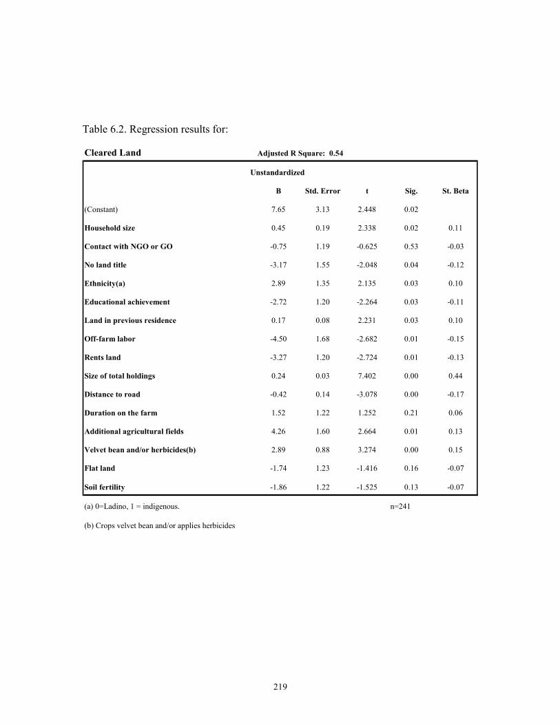
First, Cleared land (Table 6.2.) is positively related to household size, ethnicity,

having land in previous residence, size of farm holdings, having additional agricultural

fields, and use of velvet bean and/or herbicides. Cleared land is negatively associated

with lack of land title, having any formal education, off-farm labor, renting land, and

distance to road.

The standardized regression coefficient for size of total holdings is several times

larger than that of any other variable in the model. This is expected since more land

should mean more land in use. Distance to road was the second most important variable

and its sign was in the hypothesized direction, as expected, since distance from the road

decreases the incentive of production for market.

Velvet bean and/or herbicides and off-farm labor followed distance to road as the

most important variable. The sign is not in the expected direction however, suggesting

that agricultural intensification may ultimately be encouraging extensification, possibly to

free up land for cattle expansion. As expected, off-farm labor was related with less forest

clearing since time away from the farm to work elsewhere means less time can be

devoted to clearing one’s own land.

Rents land and additional agricultural fields were the next most important

variables. They were were significant at the 0.01 level and met theoretical expectations

In the first case, renters have small plots on which little total land is cleared. In the

second case, the use of an additional field (not adjacent to one’s primary farm) reflects

having cleared more land for agriculture.

The remaining five variables were significant at the 0.05 level. Lack of land title

was negatively related to forest clearing. This contradicts a large body of literature which

considers secure land title as an incentive to forest conservation. Maya were also found

to clear more forest than Ladinos. This supports some previous research in Petén, but

must be considered within the context of a relatively small sample of Maya settlers and

the fact that the sample is comprised of several different Maya groups. Approximately

half the Maya in the sample are Q’eqchí, and grouping them into one category with other

Maya groups is problematic.

Educational achievement and land in previous residence were also significant. It

appears that education is inversely related to extensification, supporting one of my

209

competing hypotheses. In the case of land in previous residence, the positive relation

meets the expectation that these farmers are either wealthier or were accustomed to

extensive farming in remote locations in their previous residence.

Lastly, household size was significant at the 0.02 level. This positive relation

controlling for other significant variables supports the notion that more family members

stimulates demand for subsistence food production while also augmenting the means to

increase production.

As forestland is the exact opposite of cleared land, the inverse relation is observed

for all variables in the model compared to cleared land, except one (Table 6.3.). Size of

total holdings, as explained above, is a very strong predictor of forest, with several times

the effect size of any other variable in the model.

Cropland (Table 6.4.) is positively associated with size of farm holdings, having

additional agricultural fields, and the use of velvet bean and/or herbicides. Cropland is

negatively related to lack of land title. In this model, lack of land title had a considerably

stronger effect than did any other predictor, including size of total holdings. This

supports one of the competing hypotheses that having legal claim to the farm is

associated with relatively more land cleared for pasture than for crops. Size of total

holdings and additional agricultural fields were the next strongest variables in the model

and supported hypotheses of agricultural extensification

An unexpected relation emerged with the use of velvet bean and/or herbicides

positively related to cropped land. This was unexpected since intensification measures

allow for more crops to be produced, reducing the need to extensify agriculture. Lastly, a

marginally positive association was observed between cropland and Maya etnicity.

Fallow land (Table 6.5.) is positively associated with household size, lack of land

title, having land in previous residence, farm size, duration, occupying additional

agricultural fields and the use of velvet bean and/or herbicides. As reported for cleared

land, size of holdings is the most important variable in the model. Rents land and

distance to road were the second most important predictors. Rents land is negative, as

hypothesized, since renters change farm plots from season to season without letting land

go fallow. This relation was clearly expected and is reflected in the relatively strong

standardized Beta coefficient. Distance to road is also an important variable and, as

210

predicted, is negatively related to fallow land since farmers further from the road may be

less market-oriented.

Lack of land title and the cropping of velvet bean or the use of herbicides are the

next most important variables and are in the expected direction, as reported in cleared

land. In the first case, the relation likely reflects that lack of title may favor crops over

cattle. Regarding the use of velvet bean and/or herbicides, the relation was hypothesized

to reduce fallow rotations. Perhaps this hypothesis was unmet because fallow land

reflects past land use while velvet bean and/or herbicides reflects current intensification

techniques. Indeed, the cropping of velvet bean could have been stimulated by the very

fact that farmers who have already cleared much of their land for crops over time, may

wish to conserve some forest as an insurance for future harvests and for bequeathing

farmland with good harvest potential to their children. Further, it is possible that farmers

are extensifying and intensifying simultaneously, as could be the case, for example, with

farmers with cattle or market-oriented farmers.

Additional agricultural fields, land in previous residence, duration on the farm,

off-farm labor, and household size were all in the expected direction with each relating to

extensification in the form of more fallow land. Lastly, as described above for cleared

land, education is negatively related to fallow land.

Having pasture (Table 6.6.) was positively associated with contact with an NGO

or GO, assets, and distance to road. Only the relation between assets and pasture met

expectations among the positive associations. Alternative hypotheses are presented

below. No land title and off-farm labor were negatively related to pasture, both meeting

expectations.

I have presented the results of the relations between independent variables and the

total amount of land devoted to each of the major land uses leading to forest clearing and

the binary outcome of pasture. Now I will briefly discuss the relation between predictors

and the relative proportion of land farmers devote to competing land uses. Since we

assume a priori that more land will be positively associated with all land uses, examining

percent of farm cleared allows for an interpretation of potential trade-offs between certain

land uses leading to forest conversion.

211

The percent of farm cleared is positively associated with household size, having

land in previous residence, renting land, duration, having additional fields, and the use of

velvet bean and/or herbicides. All but the latter of these relations were anticipated.

Percent of farm cleared is negatively associated with having attended primary school,

off-farm labor, size of farm holdings, and distance to road. It is also marginally inversely

related to soil fertility. It was uncertain what the relation would be between education

and percent of land cleared, but the remaining negative relations were anticipated. Size

of farm holdings is nearly three times as important as any other variable in the model.

The direction of the sign is, as expected, negative, the opposite of the relation with total

land cleared. Distance to road is the next most important predictor, supporting the

hypothesis that greater distance to a road makes market access more difficult,

discouraging extensification.

Following farm size and distance to the road, household size and land renting are

the next most important variables. Household size is significant at the 0.01 level and

suggests that for consumption and demand reasons, larger families clear a larger

percentage of their land. Rents land is, as anticipated, positively related to percent

cleared since renters tend to have small plots on which only crops are grown.

The remaining relations between independent variables and percent of land

cleared were significant at the 0.05 level. As found in the total land cleared model,

having attended school is negatively associated with percentage of the farm cleared,

while duration, off-farm labor, having land in previous residence, additional farm plots,

and the use of velvet bean and/or herbicides was positively related to the percentage of

the farm cleared. Lastly, soil fertility was marginally related in a negative direction with

cleared land.

I have discussed the relations between the direction and strength of predictors in

each of the models. I will now describe the relations between independent predictors and

the six land use outcomes, discussing potential relations between predictors and

agricultural extensification leading to forest clearing.

212

E. Discussion of Regression Results for Explanatory Variables

1. Demographic Factors

Household size had a significant positive association as hypothesized with most

measures of land extensification (but cropland), and a negative association with land in

forest. It is insignificantly related to having pastureland in crops. The relation is

significant (0.02 level) with cleared land and forest. However, with the key dependent

variable, percent of land cleared, it is the third strongest predictor in the model,

significant at the .01 level. The addition of one household member is associated with

nearly one-half a hectare more of land cleared and a 1% increase in percent of land

cleared. This offers support for the argument that more household members stimulate

greater demand for crops for household consumption and/or for sale to market.

2. Political-economic Factors

It was expected that contact with an NGO or other development organization

would be associated with less forest cleared, less land in fallow, crops, and pasture, and

more land in forest, assuming most such contacts were with conservation organizations.

However, this variable is significant only with pasture, and the relation is positive. This

would not be a sanguine result for the effects of conservation efforts in the region. I

speculate instead that this relation could be capturing the effect that a greater proportion

of farmers with cattle have visited credit-lending agencies (often to receive loans for

purchasing cattle). In addition, this contact may have involved contact with other non-

conservation organizations, such as agricultural development agencies.

No land title is significantly related to crops, fallow land, and pasture. Lacking

legal claim to the farm was associated with more than three fewer hectares of land

cleared, and more than two fewer hectares of land in crops.

Some legal claim to the farm, however tenuous, meant a much greater likelihood

of having pasture. A land title enables credit for purchasing cattle and is associated with

more established, wealthier households (as indicated in Table 5.15.). It was unexpected

that the relation would be negative with crops since squatter farmers were considered

more likely to have a greater proportion of land in crops relative to pasture. Apparently

this variable is capturing some of the effect of renters, none of whom have land titles.

213

Renters have very little land in general to extensify holdings. However, there may be

some problems with measurement regarding this variable since any household with

evidence that they have merely initiated the steps towards legal land titling are included

in the “land title” category.

3. Socio-economic Factors

Household socio-economic characteristics

Ethnicity is positively associated with forest clearing. Being Maya leads to an

increase of nearly three hectares of forest cleared. Although its Beta weight is lower than

several variables in the model, ethnicity is positively related with cleared land and

negatively associated with forest at the 0.05 level. This offers tentative support for the

notion that indigenous farmers are more expansive farmers than their Ladino neighbors.

However, prior work with the same sample indicated only slight differences between

Q’eqchí and Ladino land use when duration on the farm is taken into account(Carr,

forthcoming-a). This implies that non-Q’eqchí Maya may be the most land extensive of

the three groups (Ladino, Q’eqchí, and other Maya) and suggests the importance of

examining differences in land use among indigenous groups rather than combining them

all into one category. Further, the relation between ethnicity and percent of farm cleared

was insignificant.

The educational achievement of the head of household is negatively related to

agricultural extensification (total land cleared and percent cleared) and positively

associated with forest cover. Households whose head had attended school at some point

has 7% less land cleared on the farm. This contradicts the argument that education

stimulates consumption aspirations, and the motivation and ability to increase production

(Pichón, 1997; Moran 1984; Godoy, Groff et al. 1998). It supports the notion that some

minimum level of education promotes agricultural intensification, perhaps by way of

sufficient literacy to increase the likelihood of adoption of intensification techniques.

While this association could be thought to reflect that those with more education are more

likely to engage in off-farm activities, this is already controlled for by the inclusion of

off-farm work in the model. Moreover, it is unlikely since 97% of the farmers work in

agriculture primarily.

214

Having access to land to farm in the previous residence is associated with greater

levels of extensification in all of the land use variables (but cropland), corroborating the

importance of land use experience prior to migration (e.g., Almeida, 1992). Land in

previous residence is significant at the .15 level for pasture but did not noticeably

increase the goodness of fit of the entire model. Apparently, these households may not

have been as influenced as was previously expected by aspirations of clearing more land

to invest in market crops or in livestock (as found in, e.g., Almeida, 1992). That land in

previous residence is positively associated with fallow land may be suggestive of farmers

that came from previous frontier environments where land was sufficiently abundant for a

“bush fallow” crop rotation. Future research could include this as a dummy variable in

the model.

As hypothesized, off-farm labor is negatively associated with forest clearing,

percentage of land cleared, fallow, and pasture, and positively associated with forest.

Only two variables in the cleared land model had higher Beta values. Households with

heads participating in off-farm labor at some time during the year (usually a couple of

weeks total) reduced by 7% the percentage of land cleared on the farm. This supports the

theory that household heads that work off the farm have less time to invest labor in

agricultural production on their own farm (e.g., Murphy et al., 1997).

Renting land is negatively associated with cleared land and fallow, and is

positively associated with percentage of land cleared and forest, all as hypothesized.

Renters increase the percentage of cleared land on their farms by almost 10%, a large

effect. The variable is insignificant in relation to crops and pasture. In the case of a

small farmer, often an itinerant renter, fallow land is superfluous if the farmer intends to

work a plot for only a year or two. As with off-farm labor, the variable was quite

important as only two variables in the cleared land model had higher Beta values.

Farm characteristics

Size of total holdings is, as expected, far and away the strongest predictor of land

use. Size of total holdings had approximately three times the effect of any other variable

in the cleared land and percent cleared models, based on the Beta coefficients which

reflect the actual variance across each variable. Thus, in Table 6.7, on the results for

215

percent of land cleared, it has a Beta of 0.58 compared to 0.18 for distance to a road and

0.13 for household size and off-farm labor. This has a simple explanation. The larger the

farm, the more land that may be cleared for crops and that may be maintained in fallow

and in forest, but the lower the percentage of the farm that is cleared. Thus, for each

additional hectare farmers cleared one quarter of a hectare, but 1% less of the total farm

holdings. Farm size is also associated with cattle ownership at the .15 level but is not as

significant as land title and was thus excluded from the Pasture model.

Distance to road is negatively associated with cleared land and with percentage of

land cleared. Farmers cleared nearly one half a hectare less (nearly 1% of the farm) per

kilometer of distance to the road. Distance to road had the second largest effect after size

of total holdings on percent of farm cleared. This is consistent with results found in other

frontier environments such as in Ecuador, Bolivia, and Brazil (as discussed in Chapter

Two). The association is also negative with land in fallow, which was expected. Farmers

located further from the road may be less market-oriented and have been on the farm less

time than farmers closer to the road. Hence, they have had less time to clear the forest on

their farm. However, contrary to expectations, Distance to road is positively associated

with pasture, suggesting perhaps that the cost of transporting agricultural products to a

road may encourage the adoption of livestock for farmers with remote farms. After all,

unlike maize, cattle can walk themselves to the road!

Additional agricultural fields was positively related to cleared land and

percentage of land cleared, crops, and fallow (all at the 0.05 level or better), and

negatively associated with forest cover, all as expected. Occupying additional fields to

farm increased cleared land by over four hectares (with most being put in crops) and

percent of farm cleared by almost 10%. This supports the theory that ownership of an

additional field implies a desire to expand crop production. I have described above how

the process of acquiring those additional fields should lead to these effects, which should

be controlled for to determine the other relations here which are the principal ones of

interest.

As expected, duration on the farm was positively associated with percentage of

land cleared with 6% more land cleared per additional year on the farm. Duration on the

farm was also positive significantly related to fallow, as expected, with more than two

216

hectares of fallow added per year on average. It was insignificantly related to cropland

and total land cleared. It makes sense that it is more related to fallow than to cropland

(though weakly) since farmers may crop the same or similar amounts of land each year,

but in doing so over time, fallow land is accumulated. Relative to total land cleared, it

appears that other variables, notably distance to road, are reducing the significance of the

association.

The use of velvet bean and/or herbicides was positively associated with all

measures of agricultural extensification and was negatively related with forest cover.

These results are oppostite of expections. Intensification allows greater production in

less area, hence an insignificant relation with cropland. As mentioned previously,

agricultural intensification may ultimately promote extensification by allowing more land

to be sown in pasture while minimizing the contraction of grain production below a

minimally desired threshold for household consumption. The possibility that longer

duration has led to soil decline and thus increased the use of velvet bean cannot be

determined from the data.

4. Ecological Factors

Flat land and soil fertility were not significantly related to any outcome variables

at the 0.05 level, and therefore failed to meet the expectation that they would be

associated with agricultural extensification. However, there was a marginal negative

association (significant at the 0.10 level) between soil fertility and percent of land

cleared, meeting hypothesized expectations. Farmers with fertile land cleared 6% less of

their farm than did those with poor or mediocre soil. It is likely that there is little

variability in ecological conditions among the farms in the sample for either of these

factors to be highly significant. With abundant forestland remaining on most farms, soil

depletion is also not yet an issue since good yields can usually be obtained on new plots

of recently cleared land. Similarly, land abundance allows farmers to avoid cropping on

slopes that are so steep as to cause substantial erosion.

This chapter explored the separate effects of farm and household factors on the

outcomes of deforestation and land use by colonist farmers. Household size, being Maya,

217

size of total farm holdings, having land in previous residence, occupying additional

agricultural fields, and the use of intensifying techniques (but in an unexpected direction)

were all positively related to cleared land in a cross-sectional sample of farmers in the

SLNP. Household size, having land in previous residence, duration on the farm, having

additional farm fields, and the use of velvet bean and/or herbicides were positively

related to percent of the farm cleared. The R2 values for the models of cleared land and

percent of land cleared exceeded 0.50. However, when examining underlying causes of

forest clearing, it is evident that a 100% correlation exists between migration and forest

clearing. Thus an immediate prerequisite to forest clearing is the decision of farm

households to migrate to the SLNP from origin areas. Chapter seven therefore examines

out-migration to the SLNP through interviews with community leaders in municipios of

high-out-migration to the SLNP.

218

Table 6.1.Expected Associations of Predictors to Land Use

PredictorsCleared

LandPercent Cleared Fallow Forest Crops Pasture

1. Demographics factorsHousehold size + + + - + ?2. Political-economic factorsContact with an NGO ? ? ? ? ? ?No land title ? ? + ? + -3. Socioeconomic FactorsHousehold socio-economic characteristicsEthnicity(a) ? ? ? ? ? ?Educational achievement(b) ? ? ? ? ? ?Desire for cattle(c) + + + - + NALand in previous residence(d) + + + - + +Off-farm labor(e) - - - + - -Rents land - + - - - -Assets(f) + + + - + +Farm and Farming CharacteristicsSize of total holdings + - + + + +Distance to road - - - + - -Duration on the Farm + + + - + +Additional agricultural fields + + + + + +Velvet Bean and/or herbicides(g) - - - + - ?4. Ecological factorsSoil fertility - - - + + -Flat land + + + - + +a) Defined as 0 = Ladino, 1 = indigenous.b) Defined 0 = never attended school, 1 = has attended school (in reference to the household head).c) Of those without cattle, defined as 0 = do not plan to have cattle in 2008, 1 = does plan to have cattle in 2008.d) Defined as 0 = no access to land in previous residence, 1 = some access to land in previous residence.e) Defined as 0 = no participation in off-farm labor during previous 12 months, 1 = some participation in previous 12 months.f) Assets are measured such that one point each is assigned to the following items: radio, automobile, chainsaw, and horse. (g) Uses v. bean/herbicides equals: 0=no usage, 1=crops velvet bean or applies herbicides, 2=crops velvet bean and applies herbicides.

219

Table 6.2. Regression results for:

Cleared Land Adjusted R Square: 0.54

Unstandardized

B Std. Error t Sig. St. Beta

(Constant) 7.65 3.13 2.448 0.02

Household size 0.45 0.19 2.338 0.02 0.11

Contact with NGO or GO -0.75 1.19 -0.625 0.53 -0.03

No land title -3.17 1.55 -2.048 0.04 -0.12

Ethnicity(a) 2.89 1.35 2.135 0.03 0.10

Educational achievement -2.72 1.20 -2.264 0.03 -0.11

Land in previous residence 0.17 0.08 2.231 0.03 0.10

Off-farm labor -4.50 1.68 -2.682 0.01 -0.15

Rents land -3.27 1.20 -2.724 0.01 -0.13

Size of total holdings 0.24 0.03 7.402 0.00 0.44

Distance to road -0.42 0.14 -3.078 0.00 -0.17

Duration on the farm 1.52 1.22 1.252 0.21 0.06

Additional agricultural fields 4.26 1.60 2.664 0.01 0.13

Velvet bean and/or herbicides(b) 2.89 0.88 3.274 0.00 0.15

Flat land -1.74 1.23 -1.416 0.16 -0.07

Soil fertility -1.86 1.22 -1.525 0.13 -0.07

(a) 0=Ladino, 1 = indigenous. n=241

(b) Crops velvet bean and/or applies herbicides

220


Forest land Adjusted R Square: 0.77

Unstandardized


(Constant) -7.65 3.13 -2.448 0.02

Household size -0.45 0.19 -2.338 0.02 -0.08

Contact with NGO or GO 0.75 1.19 0.625 0.53 0.02

No land title 3.17 1.55 2.048 0.04 0.08

Ethnicity(a) -2.89 1.35 -2.136 0.03 -0.07

Educational achievement 2.72 1.20 2.264 0.03 0.08

Land in previous residence -0.17 0.08 -2.231 0.03 -0.07

Off-farm labor 3.27 1.20 2.724 0.01 0.09

Rents land 4.50 1.68 2.682 0.01 0.11


Distance to road 0.42 0.14 3.078 0.00 0.12

Duration on the farm -1.52 1.22 -1.252 0.21 -0.04

Additional agricultural fields -4.26 1.60 -2.664 0.01 -0.09

Velvet bean and/or herbicides(b) -2.89 0.88 -3.275 0.00 -0.11

Flat land 1.74 1.23 1.416 0.16 0.05

Soil fertility 1.87 1.22 1.526 0.13 0.05



221


Cropland Adjusted R Square: 0.22

Unstandardized


(Constant) 5.92 1.54 3.832 0.00

Household size 0.09 0.10 0.946 0.35 0.06


No land title -2.44 0.77 -3.188 0.00 -0.23

Ethnicity(a) 1.14 0.67 1.699 0.09 0.10



Off-farm labor -0.54 0.59 -0.908 0.37 -0.06

Rents land -1.30 0.83 -1.563 0.12 -0.11


Distance to road 0.00 0.07 0.012 0.99 0.00

Duration on the farm -0.34 0.60 -0.573 0.57 -0.04



Flat land -0.05 0.61 -0.088 0.93 -0.01

Soil fertility -0.15 0.60 -0.250 0.80 -0.02



222


Fallow land Adjusted R Square: 0.37

Unstandardized


(Constant) -1.33 2.66 -0.500 0.62

Household size 0.37 0.16 2.257 0.03 0.12

Contact with NGO or GO 0.27 1.01 0.268 0.79 0.01

No land title 2.70 1.32 2.052 0.04 0.14

Ethnicity(a) 1.86 1.15 1.610 0.11 0.09



Off-farm labor -2.06 1.02 -2.021 0.04 -0.11

Rents land -4.29 1.43 -3.001 0.00 -0.19


Distance to road -0.41 0.12 -3.581 0.00 -0.23




Flat land -1.24 1.04 -1.191 0.24 -0.07

Soil fertility -1.33 1.04 -1.276 0.20 -0.07



223


Pasture Nagelkerke R Square: 0.60

B S.E. Sig.

Household size 0.09 0.07 0.22

No land title -4.095 0.62 0.00

Contact with NGO or GO 1.02 0.45 0.02

Assets(a) 0.82 0.27 0.00

Off-farm labor -1.22 0.49 0.01

Distance to road 0.14 0.06 0.01

(Constant) -1.58 0.67 0.02

(a) One point each is assigned to the following items: radio, automobile, cha

224


Percent of Farm Cleared Adjusted R Square: 0.50

Unstandardized


(Constant) 0.74 0.08 9.015 0.00

Household size 0.01 0.01 2.705 0.01 0.13


No land title -0.02 0.04 -0.564 0.57 -0.03

Ethnicity(a) 0.04 0.04 1.181 0.24 0.06



Off-farm labor -0.07 0.03 -2.370 0.02 -0.12

Rents land 0.10 0.04 2.170 0.03 0.13

Size of total holdings -0.01 0.00 -9.394 0.00 -0.58

Distance to road -0.01 0.00 -3.233 0.00 -0.18




Flat land -0.01 0.03 -0.286 0.78 -0.01

Soil fertility -0.06 0.03 -1.738 0.08 -0.09



225

Figure 6.1. Mean total # of ha. cleared: No pasture vs. pasture.

0

5

10

15

20

25

No Pasture (76%) Pasture (24%)

hectares

chapter 6 - uc santa barbara geography · chapter 6 the previous chapter presented descriptive...

Documents