chapter 6 rst controller 6.1...

CHAPTER 6

RST CONTROLLER

6.1 INTRODUCTION

Usually controllers can be designed either in analog domain or

digital based on the requirement. Reference Signal Tracking (RST)

controller design is the elegant pole placement based controller among

the various methods available for linear SISO systems. Basically RST

controller has a two degree of freedom structure. The RST controller

comprises of three polynomials namely R, S & T which are usually

tuned by pole placement method. RST controller is becoming

widespread in electrical engineering application, for advanced control

such as in shunt and series active compensators used in power quality

improvement. The controller provides both feed-forward and feedback

actions. Single degree of freedom controllers like PID, IMC can

effectively are very effective in set point tracking but poor in

disturbance rejection, however, the disturbance rejection can be

obtained at the cost of reduced stability margins.

The PID and IMC controllers are basically feedback controllers as

they are placed in feedback path and modify the error signal or

feedback signal. One the major drawback of feedback controller is, it

will not process the input signal, hence cannot reject input signal

disturbance. The situations where feedback controller cannot be used,

feed-forward controller can be used. The controller is based on the

resolution of a Diophantine equation. In these early works, the authors

have dealt with rejection of low-frequency disturbances of nth order

polynomial while maintaining the closed loop gain unity. Constant

reference inputs like step signals are taken care. Later ramp type

reference signals tracking were resolved by the auxiliary Diophantine

equation. In all the early works, the design of controller is purely in

digital domain. The main drawback in the digital domain is the

selection of sampling time and errors while conversion of analog to

digital. In this chapter, RST controller design is presented in analog

domain.

6.2 OPERATION

The fig 6.1 represents the closed loop system of the process to be

controlled with RST controller [41], [42]. As seen from the fig 6.1,

Fig 6.1: closed loop system of process to be controlled with RST controller

( )

( )

B s

A s is the plant

( )

( )

R s

S s is the feedback controller

( )

( )

T s

S s is the feed-forward controller

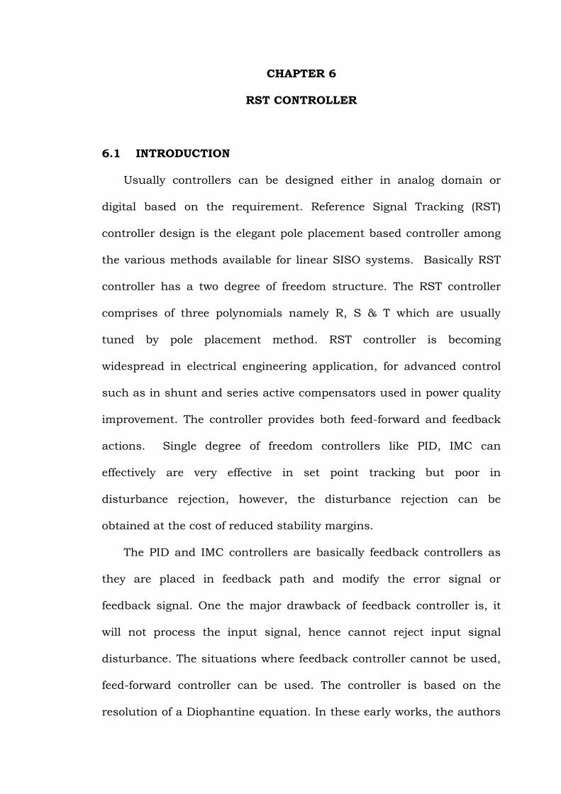
The closed loop transfer function becomes

s inv L

BT SDV V I

AS BR AS BR

(6.1)

Again there are two requirements of the controller which are specified

as:

1s

inv

V BT

V AS BR

(6.2)

0s

L

V SD

I AS BR

(6.3)

These two requirements lead to two objective functions, which have

to be satisfied. Moreover, these two constraints are depending on each

other and are related as almost inversely proportional to each other.

Hence the selection of the control parameters depends on the weightage

given to the constraint. A good solution to the problem is to apply

multi objective optimization technique for control variable selection.

Another solution is to place the poles appropriately and check the

constraints by trial and error basis.

6.3 Diophantine Equation

Given G(s), if there exists a proper compensator C(s)= R(s)/S(s) so

that all poles of E(s) can be arbitrarily assigned, the design is said to

achieve arbitrary pole placement. In the pole placement, if a complex

number is assigned as a pole, its complex conjugate must also be

assigned. The pole placement equation can be written as

( )* ( ) ( )* ( ) ( )A s S s B s R s E s (6.4)

This polynomial equation is called a Diophantine equation [43],

[44]. The crux of pole placement is solving the Diophantine equation

( )* ( ) ( )* ( ) ( )A s S s B s R s E s (6.5)

In this equation, A(s) and B(s) are known, E(s) is to be chosen by

pole placement in order to obtain R(s) and S(s) functions. If A(s) and

B(s) have common factor, then E(s) cannot be chosen arbitrarily. If does

not have any common factors, then E(s) can be chosen arbitrarily. E(s)

refers to the closed poles to be chosen so as to meet the desired

performance criteria. For proper regulation,

deg E(s) ≤ 2deg A(s)-1 (6.6)

deg T(s) ≤ deg E(s)- deg A(s) (6.7)

deg R(s) deg E(s) – deg A(s) (6.8)

deg S(s) ≤ deg R(s) (6.9)

As per the regulation criteria,

Deg E(s)=2 and can be written as

3 2

3 2 1 0( )E s E s E s E s E (6.10)

Similarly, the other polynomials can be written as

1 0( )R s R s R

(6.11)

1 0( )S s S s S (6.12)

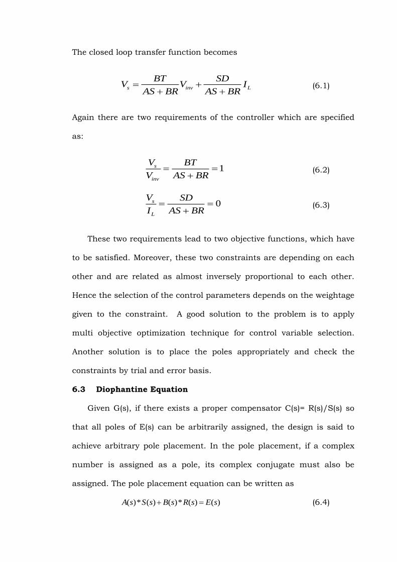
0( )T s T (6.13)

In order to choose closed loop poles, the polynomial ( )E s can be

sub classified as two components namely: 1( )E s and 2 ( )E s . 1( )E s is the

closed loop poles chosen to satisfy the desired regulation performance.

2 ( )E s is the auxiliary poles chosen either to provide filtering effects in

certain frequency region or to reduce stress on the PWM controller as

well as to improve the robustness of the closed loop system. The

control variables ( )R s , ( )S s can be calculated by the matrix called

Sylvester matrix given as:

00 0 0

11 0 0 0

22 1 1

32 1

0 0

0

0 0

0 0 0

EA B S

EA A B R

EA A S

EA R

(6.14)

6.4 THEORETICAL DESIGN

Algorithm for selection of closed loop poles

Step 1: Obtain the open loop poles of the plant.

Step 2: From the open loop poles obtain the damping factor and

natural frequency

Step 3: Fix the degree of control variables S(s) & R(s) as per the

voltage regulation criteria and obtain degree of

characteristic equation.

Step 4: If the open loop poles are complex, then atleast one pair of

closed loop poles must be complex conjugate.

Step 5: Select the real pole close to origin, and desired damping

factor

In the RST controller, the polynomial R(s) refers to zeros, affects the

overshoot and settling time in the closed loop response. The overshoot

and rise time increases as the zero moves towards the left in the s-

plane. However, the values of R(s) polynomial also correspond to

voltage regulation with disturbance rejection. The polynomial S(s)

corresponds to poles in feedback path. Values of S(s) polynomial

corresponds to stability. The stability decreases as the poles move

towards left in s-plane increasing the response.

With values of R, L & C chosen as

1R , 3L mH and 20C F

The open loop poles of the plant without controller is given as

-166 ±4079i, which represent exponentially decreasing oscillatory

response for step input. When poles are compared with standard

second order poles, corresponding damping factor and natural

frequency are obtained as 0.04 and 4082 rad/sec.

From the equation 6.11, the Ro controls the disturbance rejection

and voltage regulation; hence Ro and R1 must be multiple of natural

frequency. Ro is chosen as 7.5 times the natural frequency, i.e 107

whereas R1 is chosen as twice the natural frequency, i.e 8246

From the equation 6.12, The So controls the stability, for minimum

stability, its value is chosen nearly same as natural frequency. The

overall closed loop transfer function with selected values is given as

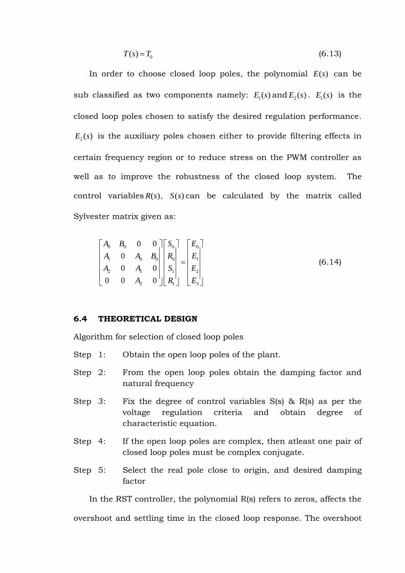
The simulink diagram of the closed loop system with disturbance is

shown in fig 6.2

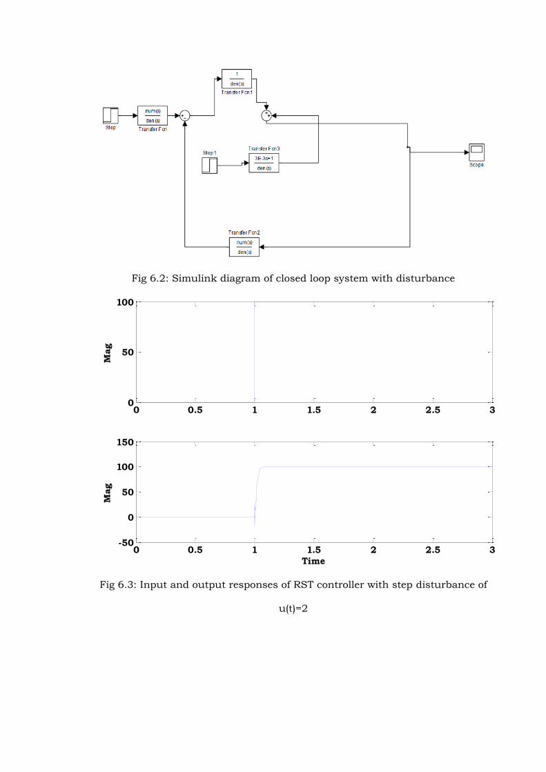
Fig 6.2: Simulink diagram of closed loop system with disturbance

0 0.5 1 1.5 2 2.5 3-50

0

50

100

150

Time

Mag

0 0.5 1 1.5 2 2.5 30

50

100

Mag

Fig 6.3: Input and output responses of RST controller with step disturbance of

u(t)=2

Bode Diagram

Frequency (rad/sec)

100

101

102

103

104

-180

-135

-90

-45

0

Ph

ase (deg)

-80

-60

-40

-20

0

Magn

itu

de (dB

)

Fig 6.4: Closed loop bode plot with RST control

Without disturbance, stability analysis is done for closed loop

system with RST controller. The fig 6.4 represents the bode plot for

closed loop system. The corresponding stability margins are:

Gain Margin : inf

Phase Margin : 1800

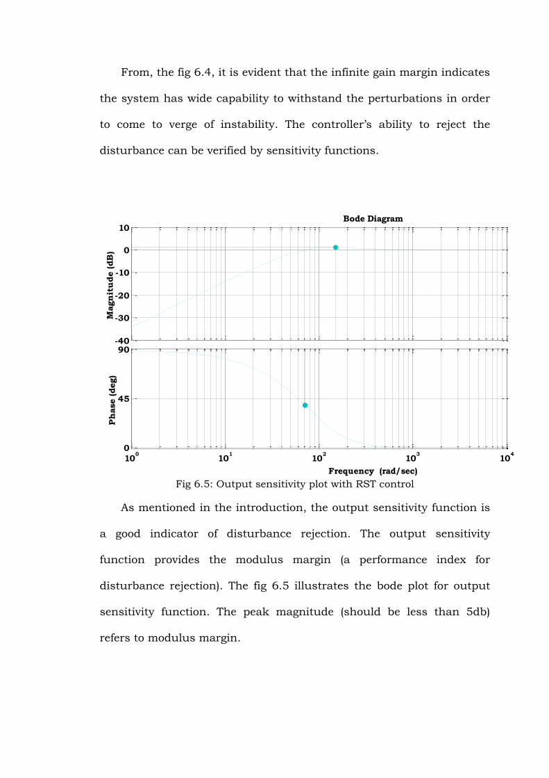
From, the fig 6.4, it is evident that the infinite gain margin indicates

the system has wide capability to withstand the perturbations in order

to come to verge of instability. The controller’s ability to reject the

disturbance can be verified by sensitivity functions.

Fig 6.5: Output sensitivity plot with RST control

As mentioned in the introduction, the output sensitivity function is

a good indicator of disturbance rejection. The output sensitivity

function provides the modulus margin (a performance index for

disturbance rejection). The fig 6.5 illustrates the bode plot for output

sensitivity function. The peak magnitude (should be less than 5db)

refers to modulus margin.

Bode Diagram

Frequency (rad/sec)

100

101

102

103

104

0

45

90

Ph

ase (deg)

-40

-30

-20

-10

0

10

Magn

itu

de (dB

)

6.5 SIMULATION RESULTS

The test system is described in chapter. In the test system, the

voltage sag is created by creating a fault with fault resistance of 0.66Ω.

This fault resistance results in 20% sag. The duration of fault is

between 0.5–0.8 secs. The voltage interruption is created by creating a

three phase fault with fault resistance of 0.001Ω. The duration of fault

is same as the voltage sag. The DVR is employed with independent dc

storage energy with open loop control. Usually DVR can mitigate voltage

fluctuation upto 50%. Research work carries study of DVR performance

in mitigating voltage interruption. Mitigation of voltage interruption

involves injection of large voltage which requires large dc energy

storage. Hence research work is carried out with open loop control for

DVR. The DVR operates during this period and its fast response to the

voltage fluctuations depends on the controller. It is observed that with

the proposed controller, DVR is able to respond to voltage sag and

interruption within 4ms. The controller performance is verified in DVR

to mitigate voltage sag & interruption. The case studies are presented

to test controller performance in the performance of DVR. The first case

study involves distribution system connected to RL Load with three

phase fault at the load end.

Case 1: Voltage sag mitigation with RST based DVR

0.4 0.5 0.6 0.7 0.8 0.9 1-1

0

1V

a(V

)

0.4 0.5 0.6 0.7 0.8 0.9 1-1

0

1

Vb(V

)

0.4 0.5 0.6 0.7 0.8 0.9 1-1

0

1

Time

Vc(V

)

Fig 6.6: Load voltage with RST control compensating voltage sag

The fig 6.6 depicts load voltage waveform with DVR injecting voltage

during the period of sag. It is evident from the fig that during the

period, load voltage is maintained at 98%. The total harmonic

distortion of load voltage is illustrated in fig 6.7

0.4 0.5 0.6 0.7 0.8 0.9 1 1.1 1.2 1.3

-0.5

0

0.5

Selected signal: 67.91 cycles. FFT window (in red): 25 cycles

Time (s)

0 1 2 3 4 5 6 7 8 9 100

0.05

0.1

0.15

Harmonic order

Fundamental (50Hz) = 0.9289 , THD= 1.66%

Mag

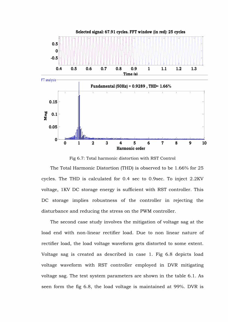
Fig 6.7: Total harmonic distortion with RST Control

The Total Harmonic Distortion (THD) is observed to be 1.66% for 25

cycles. The THD is calculated for 0.4 sec to 0.9sec. To inject 2.2KV

voltage, 1KV DC storage energy is sufficient with RST controller. This

DC storage implies robustness of the controller in rejecting the

disturbance and reducing the stress on the PWM controller.

The second case study involves the mitigation of voltage sag at the

load end with non-linear rectifier load. Due to non linear nature of

rectifier load, the load voltage waveform gets distorted to some extent.

Voltage sag is created as described in case 1. Fig 6.8 depicts load

voltage waveform with RST controller employed in DVR mitigating

voltage sag. The test system parameters are shown in the table 6.1. As

seen form the fig 6.8, the load voltage is maintained at 99%. DVR is

able to restore normal voltage at the load end within 4ms. The

corresponding Total Harmonic Distortion (THD) is found to be 1.60%

Table 6.1: Test parameters with RST controller

Parameters Values

Supply Voltage 11kV

Filter Capacitance 20µF

Filter Inductance 3mH

Filter Resistance 1

Load power factor 45deg lagging

R 8246s+10*106

S s+4170

T s + 10*106

Case 2: DVR with rectifier load for mitigation of voltage sag

0 0.2 0.4 0.6 0.8 1-1

0

1

Va(V

)

0 0.2 0.4 0.6 0.8 1-1

0

1

Vb(V

)

0 0.2 0.4 0.6 0.8 1-1

0

1

Time

Vc(V

)

Fig 6.8: Load voltage after compensation of voltage sag for rectifier load

Fig 6.9: Total harmonic distortion of load voltage

Third case study illustrates the mitigation of voltage interruption

through DVR fed with RST controller. The voltage interruption is

created for duration of 0.5sec to 0.8secs. During this voltage

interruption, DVR injects a voltage to restore the load voltage to 1pu.

However, to mitigate voltage interruption DVR requires large dc storage,

possible with independent dc storage and open loop control. The fig

6.10 represents the load voltage with DVR injecting voltage during the

period of voltage interruption. Since, DVR has to inject large magnitude

of voltage; its response is not so fast compared to voltage sag. A small

delay is observed at 0.5secs which is due to filter and PWM controller.

This delay is observed only during mitigation of voltage interruption.

However, DVR is able to mitigate voltage interruption and load voltage

0 0.2 0.4 0.6 0.8 1-1

0

1


Time (s)

0 2 4 6 8 100

0.05

0.1

0.15

0.2

Harmonic order


Mag

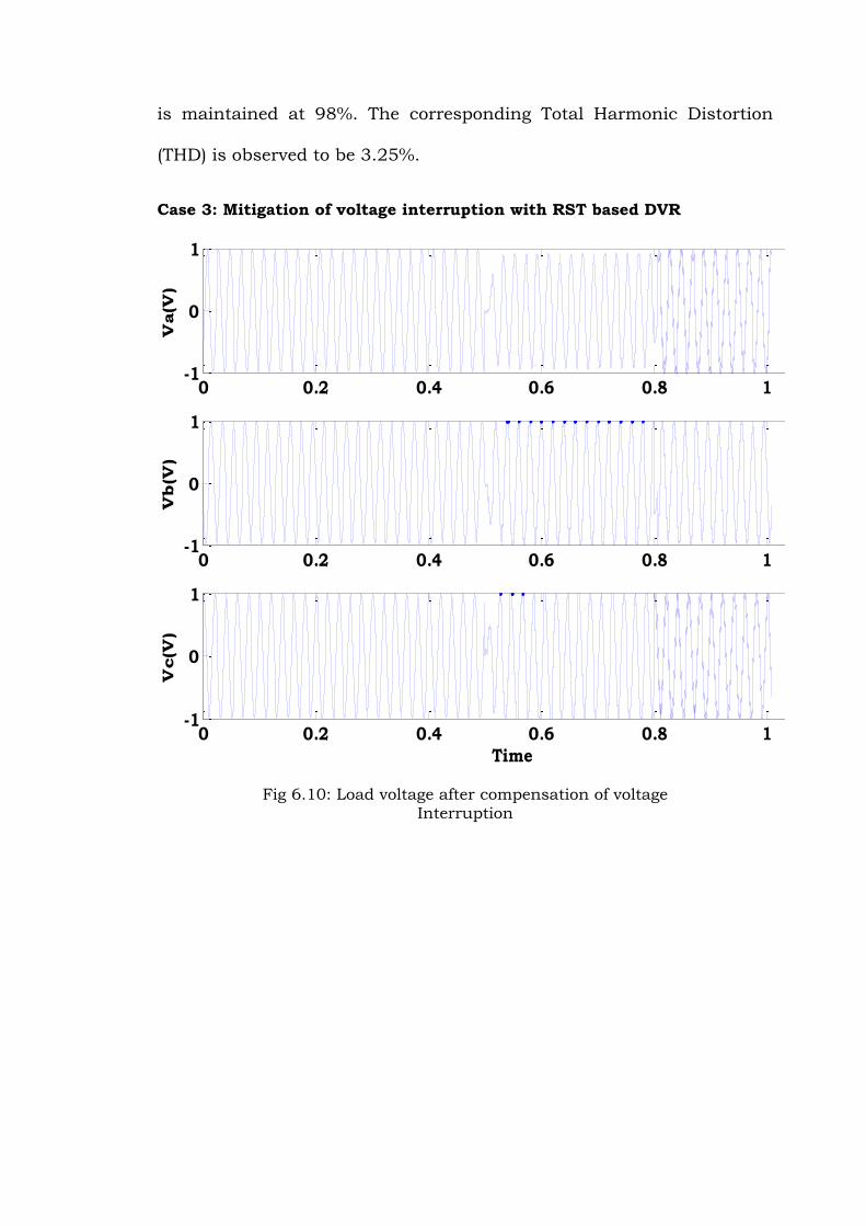
is maintained at 98%. The corresponding Total Harmonic Distortion

(THD) is observed to be 3.25%.

Case 3: Mitigation of voltage interruption with RST based DVR

0 0.2 0.4 0.6 0.8 1-1

0

1

Va(V

)

0 0.2 0.4 0.6 0.8 1-1

0

1

Vb(V

)

0 0.2 0.4 0.6 0.8 1-1

0

1

Time

Vc(V

)

Fig 6.10: Load voltage after compensation of voltage Interruption

0 0.2 0.4 0.6 0.8 1-1

0

1


Time (s)

0 2 4 6 8 100

0.1

0.2

0.3

0.4

Harmonic order


Mag

Fig 6.11: Total harmonic distortion of load voltage

Fourth case study includes the mitigation of voltage interruption

with rectifier load. The rectifier load distorts the load voltage waveform

due to its non linear nature. The DVR ability to restore the load voltage

its normal shape is verified in this case study. The fig 6.12 refers to the

load voltage with DVR injecting missing voltage with independent dc

storage energy. The DVR takes one cycle to restore the load voltage to

1pu. This delay is due to LC filter and PWM controller. However, the

load voltage is restored to 98%. The corresponding THD is observed to

3.16%.

Case 4: DVR with rectifier load for mitigation of voltage interruption

0 0.2 0.4 0.6 0.8 1-1

0

1

Va(V

)

0 0.2 0.4 0.6 0.8 1-1

0

1

Vb(V

)

0 0.2 0.4 0.6 0.8 1-1

0

1

Vc(V

)

Fig 6.12: Load voltage with RST control

0 0.2 0.4 0.6 0.8 1-1

0

1Selected signal: 54.14 cycles. FFT window (in red): 25 cycles

Time (s)

0 2 4 6 8 100

0.1

0.2

0.3

0.4

Harmonic order


Mag

Fig 6.13: Total harmonic distortion of load voltage with RST control

6.5 SUMMARY

RST controller is polynomial controller comprising of two degree

of freedom. The presence of two controllers; feed-forward

controller and feedback controller makes the RST controller two

degree of freedom.

Previous work on the RST controller is focused on digital domain.

. The main drawback in the digital domain is the selection of

sampling time and errors while conversion of analog to digital.

Diophantine equation and Sylvester matrix can be used for the

calculation of RST polynomials. Based on the type of poles of the

plant, the poles of Diophantine equation has to be chosen so as

to meet the desired targets.

In the RST controller, the values of R(s) polynomial controls the

voltage regulation and disturbance rejection whereas the values

of S(s) polynomial dictate stability.

chapter 6 rst controller 6.1...

Documents