chapter 6 numerical integration
TRANSCRIPT

Chapter �
Numerical Integration
��� Introduction
After transformation to a canonical element ��� typical integrals in the element sti�ness
or mass matrices �cf� �������� have the forms
Q �
ZZ
��
���� ��NsNTt det�Je�d�d�� ���a�
where ���� �� depends on the coe�cients of the partial di�erential equation and the
transformation to �� �cf� Section ����� The subscripts s and t are either nil� �� or
� implying no di�erentiation� di�erentiation with respect to �� or di�erentiation with
respect to �� respectively� Assuming that N has the form
NT � N�� N�� � � � � Nnp�� ���b�
then ���a� may be written in the more explicit form
Q �
ZZ
��
���� ��
�����
�N��s�N��t �N��s�N��t �N��s�Nnp�t�N��s�N��t �N��s�N��t �N��s�Nnp�t
� � �
�Nnp�s�N��t �Nnp�s�N��t �Nnp�s�Nnp�t
����� det�Je�d�d��
���c�
Integrals of the form ���b� may be evaluated exactly when the coordinate trans�
formation is linear �Je is constant� and the coe�cients of the di�erential equation are
constant �cf� Problem at the end of this section�� With certain coe�cient functions and
transformations it may be possible to evaluate ���b� exactly by symbolic integration�
however� we�ll concentrate on numerical integration because�
� it can provide exact results in simple situations �e�g�� when � and Je are constants�
and

� Numerical Integration
� exact integration is not needed to achieve the optimal convergence rate of �nite
element solutions � �� �� �� and Chapter ���
Integration is often called quadrature in one dimension and cubature in higher dimen�
sions� however� we�ll refer to all numerical approximations as quadrature rules� We�ll
consider integrals and quadrature rules of the form
I �
ZZ
��
f��� ��d�d� �nX
i��
Wif��i� �i�� ����a�
where Wi� are the quadrature rule�s weights and ��i� �i� are the evaluation points� i �
� �� � � � � n� Of course� we�ll want to appraise the accuracy of the approximate integration
and this is typically done by indicating those polynomials that are integrated exactly�
De�nition ������ The integration rule ����a� is exact to order q if it is exact when
f��� �� is any polynomial of degree q or less�
When the integration rule is exact to order q and f��� �� � Hq������� the error
E � I �nX
i��
Wif��i� �i� ����b�
satis�es an estimate of the form
E � Cjjf��� ��jjq��� ����c�
Example ������ Applying ����� to ���a� yields
Q �nX
i��
Wi���i� �i�N��i� �i�NT ��i� �i� det�Je��i� �i���
Thus� the integrand at the evaluation points is summed relative to the weights to ap�
proximate the given integral�
Problems
� A typical term of an element sti�ness or mass matrix has the form
ZZ
��
�i�jd�d�� i� j�� ��
Evaluate this integral when �� is the canonical square �� � � �� � and the
canonical right ��� unit triangle�
���� One�Dimensional Quadrature �
��� One�Dimensional Gaussian Quadrature
Although we are primarily interested in two� and three�dimensional quadrature rules�
we�ll set the stage by studying one�dimensional integration� Thus� consider the one�
dimensional equivalent of ����� on the canonical �� � element
I �
Z �
��f���d� �
nXi��
Wif��i� � E� �����
Most classical quadrature rules have this form� For example�the trapezoidal rule
I � f��� � f��
has the form ����� with n � �� W� � W� � � ��� � �� � � and
E � ��f ������
� � � ��� ��
Similarly� Simpson�s rule
I �
� f��� � �f��� � f���
has the form ����� with n � �� W� � W��� �W� � ��� ��� � �� � � �� � �� and
E � �f �iv����
��� � � ��� ��
Gaussian quadrature is preferred to these Newton�Cotes formulas for �nite element
applications because they have fewer function evaluations for a given order� With Gaus�
sian quadrature� the weights and evaluation points are determined so that the integration
rule is exact �E � �� to as high an order as possible� Since there are �n unknown weights
and evaluation points� we expect to be able to make ����� exact to order �n� � This
problem has been solved �� � and the evaluation points �i� i � � �� � � � � n� are the roots
of the Legendre polynomial of degree n �cf� Section ����� The weightsWi� i � � �� � � � � n�
called Christo�el weights� are also known and are tabulated with the evaluation points
in Table ��� for n ranging from to � A more complete set of values appear in
Abromowitz and Stegun ��
Example ������ The derivation of the two�point �n � �� Gauss quadrature rule is
given as Problem at the end of this section� From Table ��� we see that W� �W� �
and ��� � �� � �p�� Thus� the quadrature rule is
Z �
��f���d� � f���
p�� � f��
p���
This formula is exact to order three� thus the error is proportional to the fourth derivative
of f �cf� Theorem ���� Example ����� and Problem � at the end of this section��

� Numerical Integration
n ��i Wi
������� ����� ����� ������� ����� �����
� ������� ��� ��� ������ ����� �����
� ������� ����� ����� ������� ����� ������������ �� ���� ������� ����� ����
� ������� ���� ���� ����� ���� ������� �� ����� ������� ���� �����
� ������� ����� ����� ������ ����� ����������� ��� ���� ������ ���� �������� ����� ��� ������ ���� ���
����� ��� ���� ����� ����� ������� ���� �� ����� ���� ���������� ���� ���� ����� ����� ����
Table ���� Christo�el weightsWi and roots �i� i � � �� � � � � n� for Legendre polynomialsof degrees to ��
Example ������ Consider evaluating the integral
I �
Z �
�
e�x�dx �
p�
�erf�� � ������������� ������
by Gauss quadrature� Let us transform the integral to �� � using the mapping
� � �x�
to get
I �
�
Z �
��e��
������d��
The two�point Gaussian approximation is
I � �I �
� e��
����p�
��� � e��
����p�
��� ��
Other approximations follow in similar order�
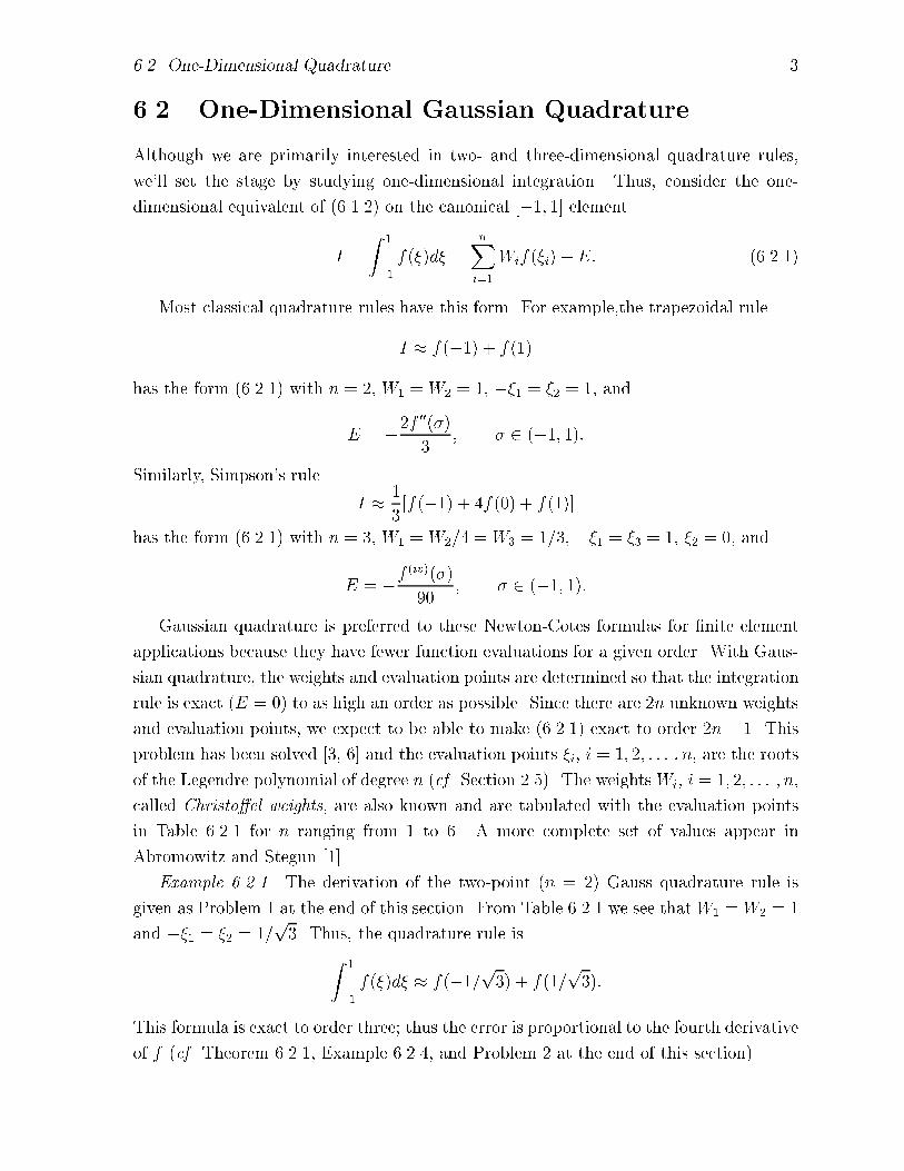
Errors I � �I when I is approximated by Gaussian quadrature to obtain �I appear in
Table ���� for n ranging from to � Results using the trapezoidal and Simpson�s rules
are also presented� The two� and three�point Gaussian rules have higher orders than the
corresponding Newton�Cotes formulas and this leads to smaller errors for this example�
���� One�Dimensional Quadrature �
n Gauss Rules Newton RulesError Error
������ ��� �������� �� ������� ��� �������� � ������ ��� ������� ��� ������ �� ��������
Table ����� Errors in approximating the integral of Example ���� by Gauss quadrature�the trapezoidal rule �n � �� right� and Simpson�s rule �n � �� right�� Numbers inparentheses indicate a power of ten�
Example ������ Composite integration formulas� where the domain of integration a� b�
is divided into N subintervals of width
�xj � xj � xj��� j � � �� � � � � N�
are not needed in �nite element applications� except� perhaps� for postprocessing� How�
ever� let us do an example to illustrate the convergence of a Gaussian quadrature formula�
Thus� consider
I �
Z b
a
f�x�dx �nX
j��
Ij
where
Ij �
Z xj
xj��
f�x�dx�
The linear mapping
x � xj��� �
�� xj
� �
�
transforms xj��� xj� to �� � and
Ij ��xj�
Z �
��f�xj��
� �
�� xj
� �
��d��
Approximating Ij by Gauss quadrature gives
Ij � �xj�
nXi��
Wif�xj��� �i�
� xj � �i�
��
We�ll approximate ������ using composite two�point Gauss quadrature� thus�
Ij ��xj�
e��xj�����xj���p���� � e��xj�����xj���
p���� ��
Numerical Integration
where xj���� � �xj � xj������ Assuming a uniform partition with �xj � �N � j �
� �� � � � � N � the composite two�point Gauss rule becomes
I �
�N
nXj��
e��xj���������Np���� � e��xj���������N
p���� ��
The composite Simpson�s rule�
I �
�N � �
N��Xi����
e�xj � �N��Xi���
e�xj � e���
on N�� subintervals of width ��x has an advantage relative to the composite Gauss rule
since the function evaluations at the even�indexed points combine�
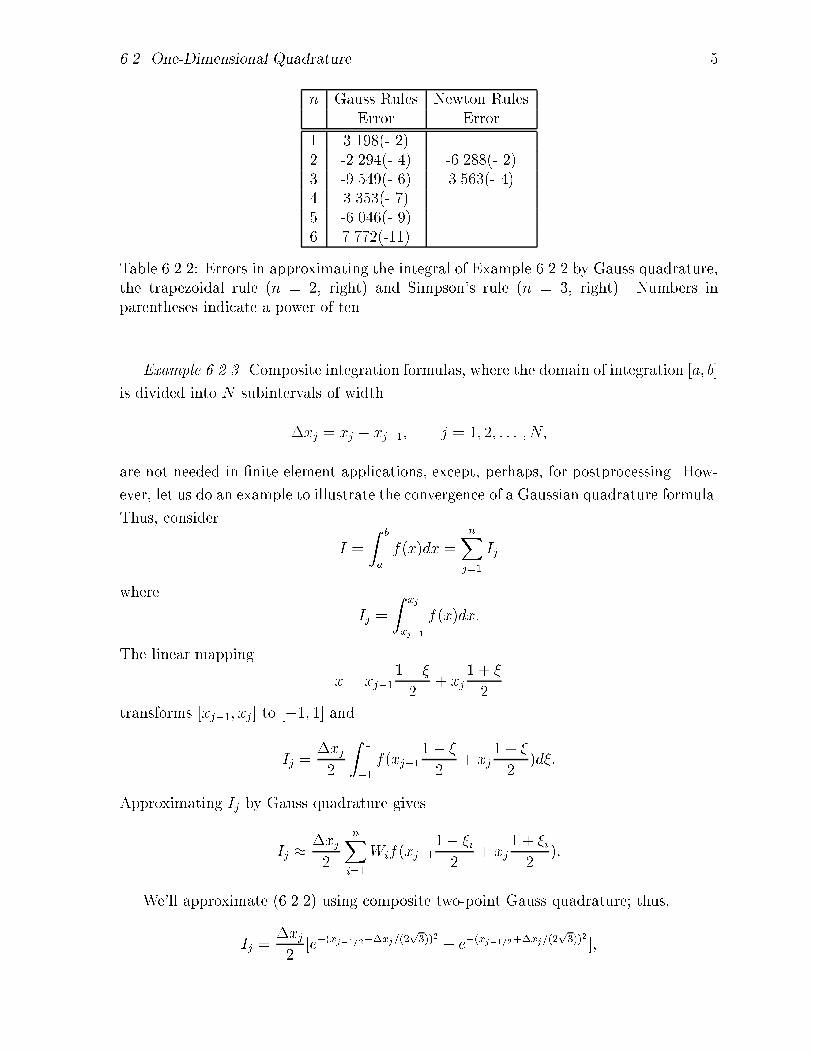
The number of function evaluations and errors when ������ is solved by the compos�
ite two�point Gauss and Simpson�s rules are recorded in Table ����� We can see that
both quadrature rules are converging as O��N� � �� Chapter ��� The computations
were done in single precision arithmetic as opposed to those appearing in Table �����
which were done in double precision� With single precision� round�o� error dominates the
computation as N increases beyond and further reductions of the error are impossible�
With function evaluations de�ned as the number of times that the exponential is evalu�
ated� errors for the same number of function evaluations are comparable for Gauss and
Simpson�s rule quadrature� As noted earlier� this is due to the combination of function
evaluations at the ends of even subintervals� Discontinuous solution derivatives at inter�
element boundaries would prevent such a combination with �nite element applications�
N Gauss Rules Simpson�s RuleFn� Eval� Abs� Error Fn� Eval� Abs� Error
� � ������� �� � ������ ��� � ���� �� � ������� ��� ������� � � ������ �� �� ������ �� � ������ ���
Table ����� Comparison of composite two�point Gauss and Simpson�s rule approxima�tions for Example ����� The absolute error is the magnitude of the di�erence betweenthe exact and computational result� The number of times that the exponential functionis evaluated is used as a measure of computational e�ort�
As we may guess� estimates of errors for Gauss quadrature use the properties of
Legendre polynomials �cf� Section ����� Here is a typical result�
���� One�Dimensional Quadrature �
Theorem ������ Let f��� � C�n �� �� then the quadrature rule ������� is exact to order
�n � if �i� i � � �� � � � � n� are the roots of Pn���� the nthdegree Legendre polynomial�
and the corresponding Christo�el weights satisfy
Wi �
P �n��i�
Z �
��
Pn���
� � �id�� i � � �� � � � � n� �����a�
Additionally� there exists a point � � ��� � such that
E �f ��n����
�n�
Z �
��
nYi��
�� � �i��d�� �����b�
Proof� cf� �� Sections ���� ��
Example ����� Using the entries in Table ��� and �����b�� the discretization error
of the two�point �n � �� Gauss quadrature rule is
E �f iv���
��
Z �
���� �
p����� � p
���d� �
f iv���
��� � � ��� ��
Problems
� Calculate the weights W� and W� and the evaluation points �� and �� so that the
two�point Gauss quadrature rule
Z �
��f�x� � W�f���� �W�f����
is exact to as high an order as possible� This should be done by a direct calculation
without using the properties of Legendre polynomials�
�� Lacking the precise information of Theorem ���� we may infer that the error in
the two�point Gauss quadrature rule is proportional to the fourth derivative of f���
since cubic polynomials are integrated exactly� Thus�
E � Cf iv���� � � ��� ��
We can determine the error coe�cient C by evaluating the formula for any function
f�x� whose fourth derivative does not depend on the location of the unknown point
�� In particular� any quartic polynomial has a constant fourth derivative� hence�
the value of � is irrelevant� Select an appropriate quartic polynomial and show that
C � ��� as in Example �����
� Numerical Integration
��� Multi�Dimensional Quadrature
Integration on square elements usually relies on tensor products of the one�dimensional
formulas illustrated in Section ��� Thus� the application of ����� to a two�dimensional
integral on a canonical �� �� �� � square element yields the approximation
I �
Z �
��
Z �
��f��� ��d�d� �
Z �
��
nXi��
Wif��i� ��d� �nX
i��
Wi
Z �
��f��i� ��d�
and
I �
Z �
��
Z �
��f��� ��d�d� �
nXi��
nXj��
WiWjf��i� �j�� �����
Error estimates follow the one�dimensional analysis�
Tensor�product formulas are not optimal in the sense of using the fewest function
evaluations for a given order� Exact integration of a quintic polynomial by ����� would
require n � � or a total of � points� A complete quintic polynomial in two dimensions
has � monomial terms� thus� a direct �non�tensor�product� formula of the form
I �
Z �
��
Z �
��f��� ��d�d� �
nXi��
Wif��i� �i�
could be made exact with only � points� The � coe�cients Wi� �i� �i� i � � �� � � � � ��
could potentially be determined to exactly integrate all of the monomial terms�
Non�tensor�product formulas are complicated to derive and are not known to very high
orders� Orthogonal polynomials� as described in Section ��� are unknown in two and
three dimensions� Quadrature rules are generally derived by a method of undetermined
coe�cients� We�ll illustrate this approach by considering an integral on a canonical right
��� triangle
I �
ZZ
��
f��� ��d�d� �
nXi��
Wif��i� �i� � E� ������
Example ������ Consider the one�point quadrature rule
ZZ
��
f��� ��d�d� � W�f���� ��� � E� ������
Since there are three unknownsW�� ��� and ��� we expect ������ to be exact for any linear
polynomial� Integration is a linear operator� hence� it su�ces to ensure that ������ is
exact for the monomials � �� and �� Thus�
���� Multi�Dimensional Quadrature �
� If f��� �� � � Z �
�
Z ���
�
��d�d� �
��W��
� If f��� �� � �� Z �
�
Z ���
�
���d�d� �
� W����
� If f��� �� � �� Z �
�
Z ���
�
���d�d� �
�W����
The solution of this system isW� � �� and �� � �� � ��� thus� the one�point quadrature
rule is ZZ
��
f��� ��d�d� �
�f�
��
�� � E� ������
As expected� the optimal evaluation point is the centroid of the triangle�
A bound on the error E may be obtained by expanding f��� �� in a Taylor�s series
about some convenient point ���� ��� � �� to obtain
f��� �� � p���� �� �R���� �� �����a�
where
p���� �� � f���� ��� � �� � ���
�� �� � ���
��f���� ��� �����b�
and
R���� �� �
� �� � ���
�� �� � ���
���f�� ��� �� �� � ��� �����c�
Integrating �����a� using ������
E �
ZZ
��
p���� �� �R���� ���d�d��
� p��
��
�� �R��
��
����
Since ������ is exact for linear polynomials
E �
ZZ
��
R���� ��d�d��
�R��
��
���
Not being too precise� we take an absolute value of the above expression to obtain
jEj �ZZ
��
jR���� ��jd�d� �
�jR��
��
��j�

� Numerical Integration
For the canonical element� j� � ��j � and j� � ��j � � hence�
jR���� ��j � � maxj�j��
jjD�f jj���
where
jjf jj��� � max��������
jf��� ��j�
Since the area of �� is ���
jEj � � maxj�j��
jjD�f jj���� �����
Errors for other quadrature formulas follow the same derivation � �� Section �����
Two�dimensional integrals on triangles are conveniently expressed in terms of trian�
gular coordinates as
ZZ
�e
f�x� y�dxdy � Ae
nXi��
Wif��i�� �
i�� �
i�� � E ������
where �� i�� �i�� �
i�� are the triangular coordinates of evaluation point i and Ae is the area of
triangle e� Symmetric quadrature formulas for triangles have appeared in several places�
Hammer et al� �� developed formulas on triangles� tetrahedra� and cones� Dunavant ��
presents formulas on triangles which are exact to order ��� however� some formulas have
evaluation points that are outside of the triangle� Sylvester �� developed tensor�product
formulas for triangles� We have listed some quadrature rules in Table ��� that also
appear in Dunavant ��� Strang and Fix ��� and Zienkiewicz ��� A multiplication factor
M indicates the number of permutations associated with an evaluation point having a
weight Wi� The factor M � is associated with an evaluation point at the triangle�s
centroid ���� ��� ���� M � � indicates a point on a median line� and M � indicates
an arbitrary point in the interior� The factor p indicates the order of the quadrature rule�
thus� E � O�hp��� where h is the maximum edge length of the triangle�
Example ������ Using the data in Table ��� with ������� the three�point quadrature
rule on the canonical triangle is
ZZ
��
f��� ��d�d� �
f����� �� �� � f��� �� ���� � f��� ���� ��� � E�
The multiplicative factor of � arises because the area of the canonical element is �� and
all of the weights are ��� The quadrature rule can be written in terms of the canonical
variables by setting �� � � and �� � � �cf� ������ and ��������� The discretization error
associated with this quadrature rule is O�h���
���� Multi�Dimensional Quadrature
n Wi � i� � i�� �i� M p
���������������� ����������������� ����������������� �����������������
� ����������������� ��� ��� ���� �
� ����������������� ����������������� ����������������� ������������������
����������������� ���������������� ���������������������������������� �
�������������� ��������������� ������������� �������������� �
������������� ������������ ������������������������������ �
� ����������������� ����������������� ����������������� ������������������
��������������� ���������������� �������������������������� �
�������������� ��������������� ������������������������ �
� ���������������� ������������ �������������� �������������� �
������������ ������������� ���������������������������� �
�������������� ������������� �����������������������������
� ��������������� ����������������� ����������������� ������������������
�������������� ��������������� ���������������������������� �
���������������� �������������� ������������������������ �
�������������� �������������� ��������������
Table ���� Weights and evaluation points for integration on triangles ���

� Numerical Integration
Quadrature rules on tetrahedra have the form
ZZZ
�e
f�x� y� z�dxdydz � Ve
nXi��
Wif��i�� �
i�� �
i�� �
i� � E ������
where Ve is the volume of Element e and �� i�� �i�� �
i�� �
i� are the tetrahedral coordinates of
evaluation point i� Quadrature rules are presented by Jinyun �� for methods to order
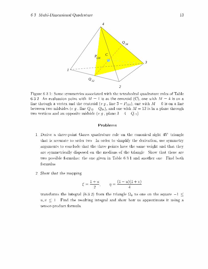
six and by Keast �� for methods to order eight� Multiplicative factors are such that
M � for an evaluation point at the centroid ���� ��� ��� ���� M � � for points on
the median line through the centroid and one vertex� M � for points on a line between
opposite midsides� M � � for points in the plane containing an edge an and opposite
midside� and M � �� for points in the interior �Figure �����
n Wi � i�� �� ��� � M p
���������������� ����������������� ����������������� ����������������� �����������������
� ����������������� ������������ ��������� ���������� ��������� �
� ������������������ ����������������� ����������������� ������������������ �����������������
����������������� ����������������� ������ ��� �
��������������� ����������������� ����������������� ������������������ �����������������
���������������� �������������� ���������������������������� �������������� �
����������������� ������������� ��������������������������� ��������������
� ���������������� ����������������� ����������������� ������������������ �����������������
������������� ����������������� ���������������������������������� ����������������� �
������������� ����������������� �������������������������������� ���������������� �
����������� ������������ �������������������������� ��������������
Table ����� Weights and evaluation points for integration on tetrahedra �� ���
���� Multi�Dimensional Quadrature �
���������������������������������������������������������������������������������������������������������������������������������������������������������������������������������������������������������������������������������������
���������������������������������������������������������������������������������������������������������������������������������������������������������������������������������������������������������������������������������������
��������
1
2
3
4
P C124
12
34
Q
Q
Figure ���� Some symmetries associated with the tetrahedral quadrature rules of Table����� An evaluation point with M � is at the centroid �C�� one with M � � is on aline through a vertex and the centroid �e�g�� line �� P���� one with M � is on a linebetween two midsides �e�g�� line Q�� �Q��� and one with M � � is in a plane throughtwo vertices and an opposite midside �e�g�� plane �� ��Q���
Problems
� Derive a three�point Gauss quadrature rule on the canonical right ��� triangle
that is accurate to order two� In order to simplify the derivation� use symmetry
arguments to conclude that the three points have the same weight and that they
are symmetrically disposed on the medians of the triangle� Show that there are
two possible formulas� the one given in Table ��� and another one� Find both
formulas�
�� Show that the mapping
� � � u
�� � �
�� u�� � v�
�
transforms the integral ������ from the triangle �� to one on the square � �u� v � � Find the resulting integral and show how to approximate it using a
tensor�product formula�

� Numerical Integration
Bibliography
� M� Abromowitz and I�A� Stegun� Handbook of Mathematical Functions� volume ��
of Applied Mathematics Series� National Bureau of Standards� Gathersburg� ���
�� S�C� Brenner and L�R� Scott� The Mathematical Theory of Finite Element Methods�
Springer�Verlag� New York� ����
�� R�L� Burden and J�D� Faires� Numerical Analysis� PWS�Kent� Boston� �fth edition�
����
�� D�A� Dunavant� High degree e�cient symmetrical Gaussian quadrature rules for the
triangle� International Journal of Numerical Methods in Engineering� ��������
����
�� P�C� Hammer� O�P� Marlowe� and A�H� Stroud� Numerical integration over simplexes
and cones� Mathematical Tables and other Aids to Computation� �������� ���
� E� Isaacson and H�B� Keller� Analysis of Numerical Methods� John Wiley and Sons�
New York� ��
�� Y� Jinyun� Symmetric Gaussian quadrature formulae for tetrahedronal regions�
Computer Methods in Applied Mechanics and Engineering� ����������� ����
�� P� Keast� Moderate�degree tetrahedral quadrature formulas� Computer Methods in
Applied Mechanics and Engineering� ����������� ���
�� G� Strang and G� Fix� Analysis of the Finite Element Method� Prentice�Hall� En�
glewood Cli�s� ����
�� P� Sylvester� Symmetric quadrature formulae for simplexes� Mathematics of Com
putation� ��������� ����
� R� Wait and A�R� Mitchell� The Finite Element Analysis and Applications� John
Wiley and Sons� Chichester� ����
�

Numerical Integration
�� O�C� Zienkiewicz� The Finite Element Method� McGraw�Hill� New York� third
edition� ����